The axial-vector contributions in two-photon reactions: pion transition form factor and deeply-virtual Compton scattering at NNLO in QCD

Abstract

Using the approach based on conformal symmetry we calculate the two-loop coefficient function for the axial-vector contributions to two-photon processes in the $\overline{\rm MS}$ scheme. This is the last missing element for the complete next-to-next-to-leading order (NNLO) calculation of the the pion transition form factor $\gamma^{\ast}\gamma\to\pi$ in perturbative QCD. The corresponding high-statistics measurement is planned by the Belle II collaboration and will allow one to put strong constraints on the pion light-cone distribution amplitude. The calculated NNLO corrections prove to be rather large and have to be taken into account. The same coefficient function determines the contribution of the axial-vector generalized parton distributions to deeply-virtual Compton scattering (DVCS) which is investigated at the JLAB 12 GeV accelerator, by COMPASS at CERN, and in the future will be studied at the Electron Ion Collider EIC.

A wealth of data on hard exclusive reactions from a new generation of experimental facilities will become available in the coming decade. These data are expected to have a very high precision and to provide a much deeper insight in the hadron structure as compared to the current knowledge. A pressing question is, however, whether hard exclusive hadronic reactions are under sufficient theoretical control to allow for fully quantitative predictions, which is highly relevant for all future high-intensity experiments. To give an example, the $\gamma^{\ast}\gamma\to\pi$ transition form factor is widely regarded as the “golden mode” that allows one to access the pion wave function at small transverse separations, usually referred to as the light-cone distribution amplitude (LCDA). The measurements of this form factor at space-like momentum transfers in the interval $4-40\,\text{GeV}^{2}$ by the BaBar Aubert et al. (2009) and Belle Uehara et al. (2012) collaborations caused much excitement and a flurry of theoretical activity due to the unexpected large scaling violation observed by Babar. At Belle II Altmannshofer et al. (2019), the statistical uncertainty is expected to be reduced by a factor of 8 and the total systematic uncertainty is estimated to be at least 2 times smaller than that at Belle due to an improved trigger efficiency. As the result, a factor 3 to 5 times more precise measurements are possible in the high-$Q^{2}$ region.

Another example is provided by DVCS which is an important part of the physics program at the JLAB 12 GeV upgrade Dudek et al. (2012), is measured also at CERN by COMPASS Akhunzyanov et al. (2019), and in the future will be studied at the EIC Accardi et al. (2016); Abdul Khalek et al. (2021). This reaction is the primary source of information on the generalized parton distributions (GPDs) of the nucleon (and, eventually, nuclei) which describe the correlation between parton’s longitudinal momentum and its position in the transverse plane. Also in this case, the accuracy of the arriving and expected data is much higher as compared to the theoretical predictions available.

In both cases the theory framework is provided by collinear factorization and, despite obvious differences, there are some common elements. In particular the scale dependence of the LCDAs and GPDs is governed by similar equations, and the coefficient function (CF) appearing in the factorized expression for the $\pi\gamma^{\ast}\gamma$ form factor in terms of the pion LCDA is the same as the CF of the axial GPD in DVCS. The corresponding calculations have to be advanced to NNLO accuracy that has become standard in studies of inclusive processes and, since recently, also in semi-inclusive reactions in the framework of transverse momentum dependent factorization Gutierrez-Reyes et al. (2018).

The new contribution of this work is a calculation of the two-loop CF for the flavor-nonsinglet axial-vector contributions in processes with one real and one virtual photon. When combined with the three-loop anomalous dimensions calculated in Braun et al. (2017), this result allows for the complete NNLO evaluation of the pion transition form factor and all flavor-nonsinglet contributions to DVCS. In this letter we concentrate ourselves in the discussion of the numerical impact of the NNLO correction on $\pi\gamma^{\ast}\gamma$, since the DVCS observables are more complicated and require a dedicated study.

The pion transition form factor with one real and one virtual photon, $F(Q^{2})\equiv F_{\pi\gamma^{*}\gamma}(Q^{2})$, can be defined by the matrix element of the time-ordered product of two electromagnetic currents

$$\int d^{4}y\,e^{iqy}\langle\pi^{0}(p)|T\{j^{\rm em}_{\mu}(y)j^{\rm em}_{\nu}(0)\}|0\rangle=$$

$$\hskip 85.35826pt=ie^{2}\varepsilon_{\mu\nu\alpha\beta}q^{\alpha}p^{\beta}F(Q^{2})\,,$$ (1)

where $e$ is the electric charge, $p$ the pion momentum, and $j^{\rm em}_{\mu}=e_{u}\bar{u}\gamma_{\mu}u+e_{d}\bar{d}\gamma_{\mu}d+\ldots.$ We will consider the space-like form factor, $Q^{2}=-q^{2}>0$. The leading contribution ${\mathcal{O}}(1/Q^{2})$ to this form factor can be written in the factorized form Lepage and Brodsky (1979, 1980)

$$F(Q^{2})=\frac{\sqrt{2}f_{\pi}}{6Q^{2}}\!\int_{0}^{1}\!dz\,\mathrm{T}(z,Q,\mu)\phi_{\pi}(z,\mu)\,,$$ (2)

where $f_{\pi}=131\leavevmode\nobreak\ \text{MeV}$ denotes the pion decay constant, $\mu$ the factorization scale, $\mathrm{T}(z,Q,\mu)$ the CF and $\phi_{\pi}(z,\mu)$ the pion LCDA normalized as $\int_{0}^{1}dz\,\phi_{\pi}(z,\mu)=1$ .

The same CF enters the axial-vector contributions to the DVCS amplitude $\mathcal{A}_{\mu\nu}=g_{\mu\nu}^{\perp}\mathcal{V}+\epsilon_{\mu\nu}^{\perp}\mathcal{A}$

$$\mathcal{A}(\xi,Q^{2})=\frac{1}{2}\sum_{q}e_{q}^{2}\int\limits_{-1}^{1}\!\frac{dx}{\xi}\mathrm{T}\Big{(}\tfrac{\xi-x}{2\xi},Q,\mu\Big{)}\widetilde{F}_{q}(x,\xi,t,\mu)\,,$$ (3)

where $\widetilde{F}_{q}(x,\xi,t,\mu)$ is the axial-vector GPD and $\xi$ is the skewedness parameter, see Diehl (2003); Belitsky and Radyushkin (2005) for details. Here it is assumed that $\mathrm{T}(\tfrac{\xi-x}{2\xi},Q^{2},\mu)$ is continued analytically to the $|x/\xi|>1$ region using the $\xi\to\xi-i\epsilon$ prescription.

The CF can be expanded in powers of the strong coupling, $a_{s}=\alpha_{s}(\mu)/4\pi$,

$$\mathrm{T} =\mathrm{T}^{(0)}+a_{s}\mathrm{T}^{(1)}+a^{2}_{s}\mathrm{T}^{(2)}+\ldots$$ (4)

The first two terms in this series are well known Lepage and Brodsky (1980); del Aguila and Chase (1981); Braaten (1983); Kadantseva et al. (1986)

$$\mathrm{T}^{(0)}(z) ={1}/{z}+{1}/{\bar{z}}\,,$$ (5)

$$\mathrm{T}^{(1)}(z,Q,\mu) =C_{F}\frac{1}{z}\Big{[}\ln^{2}z-\frac{z\ln z}{\bar{z}}-9+\left(3+2\ln z\right)\mathrm{L}\Big{]}$$

$$\quad+(z\leftrightarrow\bar{z})\,,$$ (6)

where $\bar{z}=1-z$ and $\mathrm{L}=\ln(Q^{2}/\mu^{2})\,.$ The two-loop correction $\mathrm{T}^{(2)}$ is the subject of this work. It can be decomposed in the contributions of three color structures:

$$\mathrm{T}^{(2)} =C_{F}^{2}\mathrm{T}^{(2)}_{\rm P}+\frac{C_{F}}{N_{c}}\mathrm{T}^{(2)}_{\rm NP}+\beta_{0}C_{F}\mathrm{T}^{(2)}_{\beta}\,,$$ (7)

where $C_{F}=(N_{c}^{2}-1)/2N_{c}$ and $\beta_{0}=11/3N_{c}-2/3n_{f}$ in a $\mathrm{SU}(N_{c})$ gauge theory. We obtain (for $\mu=Q$)

$$\mathrm{T}^{(2)}_{\rm P} =\biggl{\{}\frac{2}{z}\Big{(}6\mathrm{H}_{0000}-\mathrm{H}_{1000}-2\mathrm{H}_{200}-\mathrm{H}_{1100}-\mathrm{H}_{120}-\mathrm{H}_{210}+\mathrm{H}_{1110}\Big{)}+\frac{2}{\bar{z}}\mathrm{H}_{000}-\frac{8}{z}\mathrm{H}_{100}+\frac{2}{\bar{z}}\mathrm{H}_{20}+\frac{4}{z}\mathrm{H}_{110}$$

$$\quad-\left(\frac{11}{\bar{z}}+\frac{38}{3z}\right)\mathrm{H}_{00}+\frac{34}{3z}\mathrm{H}_{10}+\frac{2}{z}\zeta_{2}\Big{(}\mathrm{H}_{11}-\mathrm{H}_{2}-\mathrm{H}_{10}-4\mathrm{H}_{00}\Big{)}-\frac{1}{\bar{z}}\left(2\zeta_{2}-4\zeta_{3}-\frac{71}{2}\right)\mathrm{H}_{0}$$

$$\quad+\frac{1}{z}\left(6\zeta_{2}+32\zeta_{3}-\frac{64}{9}\right)\mathrm{H}_{0}+\frac{1}{z}\left(\frac{701}{24}+\frac{34}{3}\zeta_{2}+43\zeta_{3}+3\zeta_{2}^{2}\right)\biggr{\}}+(z\leftrightarrow\bar{z})\,,$$ (8)

$$\mathrm{T}^{(2)}_{\mathrm{NP}} =\biggl{\{}12\left(\mathrm{H}_{20}+\mathrm{H}_{110}-\frac{1}{z}\mathrm{H}_{10}-\frac{1}{\bar{z}}\mathrm{H}_{0}-\zeta_{3}\right)-\frac{6}{z}\mathrm{H}_{200}-\left(\frac{2}{\bar{z}}+\frac{4}{z}\right)\Big{(}\mathrm{H}_{30}+\mathrm{H}_{210}+\mathrm{H}_{31}\Big{)}+\left(\frac{2}{\bar{z}}+\frac{8}{z}\right)\mathrm{H}_{4}$$

$$\quad+\left(\frac{4}{\bar{z}}+\frac{6}{z}\right)\mathrm{H}_{22}+\frac{6}{\bar{z}}\Big{(}\mathrm{H}_{3}-\mathrm{H}_{20}\Big{)}+\left[\frac{2}{\bar{z}}\left(1-\zeta_{2}\right)+\frac{4}{z}\left(\frac{2}{3}-\zeta_{2}\right)\right]\mathrm{H}_{00}-\left[\frac{4}{z}\left(\zeta_{2}-1\right){-\frac{1}{\bar{z}}\left(\frac{38}{3}-2\zeta_{2}\right)}\right]\mathrm{H}_{2}$$

$$\quad+\left[\frac{1}{z}\left(14\zeta_{3}-\frac{32}{9}\right)+\frac{1}{\bar{z}}\left(1-6\zeta_{2}+6\zeta_{3}\right)\right]\mathrm{H}_{0}-\frac{1}{z}\left(3\zeta_{2}^{2}+20\zeta_{2}-36\zeta_{3}+\frac{73}{12}\right)\biggr{\}}+(z\leftrightarrow\bar{z})\,,$$ (9)

$$\mathrm{T}^{(2)}_{\beta} =\biggl{\{}-\frac{2}{z}\mathrm{H}_{000}+\frac{2}{z}\mathrm{H}_{100}-\frac{1}{z}\mathrm{H}_{110}+\left(\frac{10}{3z}-\frac{1}{\bar{z}}\right)\mathrm{H}_{00}-\frac{14}{3z}\mathrm{H}_{10}+\left[\frac{1}{\bar{z}}\left(\frac{1}{2}+\zeta_{2}\right)-\frac{19}{9z}\right]\mathrm{H}_{0}$$

$$\quad-\frac{1}{z}\left(\zeta_{3}+\frac{14}{3}\zeta_{2}+\frac{457}{24}\right)\biggr{\}}+(z\leftrightarrow\bar{z})\,,$$ (10)

where $\mathrm{H}_{\vec{m}}=\mathrm{H}_{\vec{m}}(z)$ are harmonic polylogarithms Remiddi and Vermaseren (2000). Our result for $\mathrm{T}^{(2)}_{\beta}$ is in agreement with Ref. Melic et al. (2002). The expressions for $\mathrm{T}^{(2)}_{\mathrm{P}}$ (planar), $\mathrm{T}^{(2)}_{\mathrm{NP}}$ (nonplanar) are new results. Complete results for $\mathrm{T}^{(2)}(z,\mu)$ in Mathematica format are presented in the ancillary file.

Our method of calculation is based on using conformal symmetry of QCD at critical coupling in $d=4-2\epsilon$ dimensions to relate the CF in question to the well-known two-loop axial-vector CF in deep-inelastic scattering Zijlstra and van Neerven (1994); Moch and Vermaseren (2000). A similar idea was used before in Ref. Melic et al. (2003) where the NNLO CF was calculated in a special, conformal renormalization scheme. Our technique is explained in detail in Ref. Braun et al. (2020) where the vector CF was calculated by the same method. The generalization to axial-vector operators is considered in Ref. Braun et al. (2021). Thus in what follows we will only outline the main steps and omit technical details.

The starting point is that QCD at the Wilson-Fischer critical point at noninteger $d=4-2\epsilon^{*}$ space-time dimensions, $\epsilon^{\ast}=-\beta_{0}a_{s}-\beta_{1}a_{s}^{2}+\ldots\$, is a conformal theory. The strategy is to calculate the CF in conformal QCD, and go over to the “physical” limit $\epsilon\to 0$ at the very end, by adding a term $\sim\epsilon^{\ast}$:

$$\mathrm{T}=\mathrm{T}_{\ast}+\epsilon^{\ast}\Delta\mathrm{T}\,.$$ (11)

The extra term $\Delta\mathrm{T}$ requires a one-loop calculation and only affects $\mathrm{T}^{(2)}_{\beta}$.

Figure 1: The ratios $T_{\rm NLO}/T_{\rm LO}$, $T_{\rm NNLO}/T_{\rm LO}$, and $T_{\rm NNLO}/T_{\rm NLO}$ at the scale $Q^{2}=\mu^{2}=4\,\mathrm{GeV}^{2}$. Here $T_{\rm LO}=T^{(0)}$, $T_{\rm NLO}=T^{(0)}+a_{s}T^{(1)}$ and $T_{\rm NNLO}=T^{(0)}+a_{s}T^{(1)}+a_{s}^{2}T^{(2)}$ are the CFs defined in (4) truncated at the first (tree level), second (one-loop) and third (two-loop) terms, respectively. For this calculation we used $\alpha_{s}(\mu=2\,\text{GeV})=0.3009$ and $n_{f}=4$.

We define axial-vector operators in $d=4-2\epsilon$ dimensions using a variant of Larin’s scheme Larin (1993) for the $\gamma_{5}$ matrix, see ref. Braun et al. (2021). In $d=4$ the axial-vector operators in this scheme can be rotated to the $\overline{\rm MS}$ scheme which is defined by the condition that the vector- and axial-vector flavor-nonsinglet operators satisfy the same evolution equation.

The CF in the $\overline{\rm MS}$ scheme can be written in the form Braun et al. (2020),

$$\mathrm{T}_{\ast} =\mathrm{T}^{(0)}\otimes K\otimes e^{\mathbb{X}}\otimes\mathcal{U}^{-1},$$ (12)

where $\mathrm{T}^{(0)}$ is the tree-level CF, $e^{\mathbb{X}}$ takes into account the conformal anomaly Braun et al. (2016, 2021), $\mathcal{U}$ is the rotation operator from Larin’s scheme to the $\overline{\rm MS}$ scheme Braun et al. (2021), and $K$ is a certain $\mathrm{SL}(2)$-invariant operator (i.e., $K$ commutes with the generators of conformal transformations). The eigenvalues of $K$ can be related to the moments of the axial vector CF in deep-inelastic scattering Zijlstra and van Neerven (1994); Moch and Vermaseren (2000) up to some additional factors, cf. Eq. (3.59) in Ref. Braun et al. (2020). We have calculated these eigenvalues in terms of harmonic sums using computer algebra packages Vermaseren (1999); Ablinger (2009, 2014). The result satisfies the reciprocity relation Basso and Korchemsky (2007); Alday et al. (2015): the asymptotic expansion of the eigenvalues of $K$ at large spin $N$ is symmetric under the substitution $N\to-N-1$. This property provides a nontrivial test of the calculation.

Any $\mathrm{SL}(2)$ invariant operator is uniquely defined by its spectrum. Thus $K$ can be restored, and it remains to do the convolutions in Eq. (12) to obtain the final result. A direct evaluation of the convolution in momentum space at two loops is very cumbersome, but it can be bypassed, as explained in Ref. Braun et al. (2020), using a position-space representation at the intermediate step. In this way one ends up with much simpler integrals that we have calculated with the help of the HyperInt package Panzer (2015).

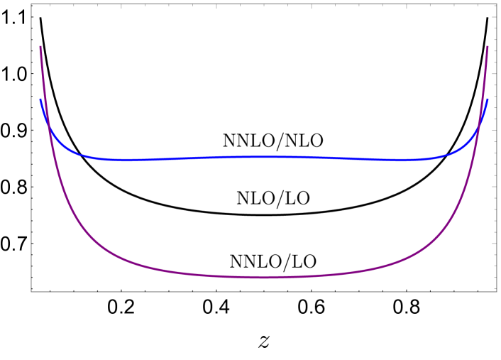
The ratios of the NLO/LO, NNLO/LO and NNLO/NLO CFs at the scale $Q^{2}=\mu^{2}=4\,\mathrm{GeV}^{2}$ are plotted in Fig. 1. One sees that the two-loop $\mathcal{O}(a^{2}_{s})$ correction has the same sign and is roughly factor two smaller as compared to the one-loop contribution in the bulk of the $z$ region. The largest contribution to $\mathrm{T}^{(2)}$ comes from $\mathrm{T}_{\beta}$ except for the endpoint regions where the leading effect is due to the Sudakov-like double-logarithmic corrections

$$\mathrm{T}(z,a_{s}) \underset{z\mapsto 0}{\simeq}\frac{1}{z}\Big{(}1+C_{F}a_{s}\ln^{2}z+\frac{(C_{F}a_{s})^{2}}{2}\ln^{4}z+\ldots\Big{)}.$$

The series likely exponentiates resulting in $\mathrm{T}(z,a_{s})\sim z^{-1+a_{s}C_{F}\ln z}$.

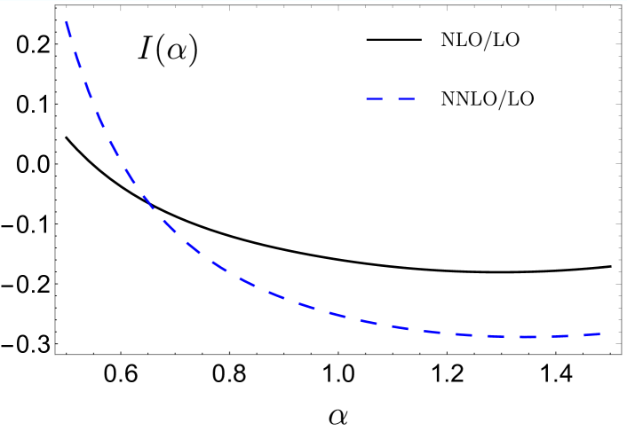
Note that also the sign of the correction changes, so that the resulting effect on physics observables will depend strongly on the behavior of the parton distributions at the endpoints. As an illustration, we show in Fig. 2 the ratios $I_{NLO}/I_{LO}$ and $I_{NNLO}/I_{LO}$ for the integral

$$I(\alpha)=\int_{0}^{1}\!dz\,z^{\alpha}\bar{z}^{\alpha}\,\mathrm{T}(z,Q^{2},\mu^{2}=Q^{2})$$ (13)

as a function of $\alpha$ in the interval $0.5<\alpha<1.5$.

Figure 2: The NNLO/LO and NLO/LO ratios for the integral $I(\alpha)$ in Eq. (13) as a function of $\alpha$.

The pion LCDA is usually represented by the expansion in terms of Gegenbauer polynomials which are eigenfunctions of the one-loop evolution equations

$$\phi_{\pi}(z,\mu) =6z\bar{z}\sum_{n=0,2,\ldots}a_{n}(\mu)C_{n}^{3/2}(2z-1).$$ (14)

Here $a_{0}=1$ is fixed by the normalization condition, and $a_{2}$ is known from lattice calculations. We use the latest result Bali et al. (2019)

$$a_{2}(\mu_{0}=2\,\text{GeV}) =0.116^{+19}_{-20}\,.$$ (15)

For the coefficients $a_{n}$ with $n>2$ there exist only very weak constraints. In order to estimate their influence, following Bali et al. (2019), we consider two models for the pion LCDA (at the scale $\mu_{0}=2\,\text{GeV}$)

$$\phi^{(I)}_{\pi}(z,\mu_{0}) =6z(1-z)[1+a_{2}(\mu_{0})C^{3/2}(2z-1)]\,,$$

$$\phi^{(II)}_{\pi}(z,\mu_{0}) =B(1+\alpha,1+\alpha)z^{\alpha}(1-z)^{\alpha}\,,$$ (16)

where the parameter $\alpha$ in the second model is adjusted to reproduce the same value of the second Gegenbauer coefficient $a_{2}$ as in Eq. (15); $B(a,b)$ is Euler’s $\beta$-function.

Using the expansion in Eq. (14) the $\pi\gamma^{\ast}\gamma$ form factor to leading-twist accuracy is given by

$$Q^{2}F(Q^{2}) ={\sqrt{2}f_{\pi}}\sum_{n=0,2,\ldots}a_{n}(\mu)c_{n}(\mu,\mathrm{L})\,,$$ (17)

where the coefficients

$$c_{n}(\mu,\mathrm{L}) =1+a_{s}c_{n}^{(1)}(\mu,\mathrm{L})+a^{2}_{s}c_{n}^{(2)}(\mu,\mathrm{L})+\ldots$$ (18)

are given by the Gegenbauer moments of the CF $\mathrm{T}(z,Q,\mu)$ in Eq. (4). The one-loop coefficients read

$$c_{n}^{(1)} =C_{F}\Big{\{}4S_{1}^{2}(n\!+\!1)-\frac{4S_{1}(n\!+\!1)-3}{(n\!+\!1)(n\!+\!2)}+\frac{2}{(n\!+\!1)^{2}(n\!+\!2)^{2}}$$

$$\quad-9-2\left[S_{1}(n\!+\!2)+S_{1}(n)-\frac{3}{2}\right]\mathrm{L}\Big{\}},$$ (19)

where $S_{1}(n)$ are the standard harmonic sums, and the first few two-loop coefficients are given by

$$c_{0}^{(2)} =-197.40+9.66\,n_{f}+\mathrm{L}\,\big{(}68.50-2.92\,n_{f}\big{)},$$

$$c_{2}^{(2)} =95.97-17.44\,n_{f}+\mathrm{L}\,\big{(}-178.25+10.9\,n_{f}\big{)}$$

$$\quad+\mathrm{L}^{2}\,\big{(}45.99-1.85\,n_{f}\big{)},$$

$$c_{4}^{(2)} =526.97-43.81\,n_{f}+\mathrm{L}\,\big{(}-417.06+20.42\,n_{f}\big{)}$$

$$\quad+\mathrm{L}^{2}\,\big{(}77.20-2.67\,n_{f}\big{)},$$

$$c_{6}^{(2)} =986.91-67.14\,n_{f}+\mathrm{L}\,\big{(}-663.97+27.73\,n_{f}\big{)}$$

$$\quad+\mathrm{L}^{2}\,\big{(}101.63-3.26\,n_{f}\big{)}.$$ (20)

In these expressions we included the logarithmic contributions, $\mathrm{L}=\ln Q^{2}/\mu^{2}$, to allow for the study of the factorization scale dependence. Note that the radiative corrections (both one-loop and two-loop) to the leading contribution $n=0$ (asymptotic LCDA) are negative, whereas the corrections to the contributions of higher moments are positive and increase with $n$. Thus the radiative corrections to the form factor in general amplify the contributions of higher-order Gegenbauer polynomials at high photon virtualities.

Figure 3: The $\pi\gamma^{\ast}\gamma$ form factor at the NNLO (solid curves) and NLO (dashed curves) in QCD perturbation theory for the two models of the pion LCDA in Eq. (16). The experimental data are from CLEO Gronberg et al. (1998) (green, open triangles), BaBar Aubert et al. (2009) (light blue, circles) and Belle Uehara et al. (2012) (dark blue, squares). In addition, the expectation for the error bars achievable at Belle II Altmannshofer et al. (2019) is shown in red. The central value for the red boxes is arbitrary.

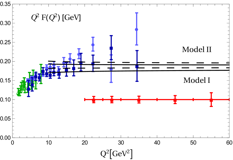
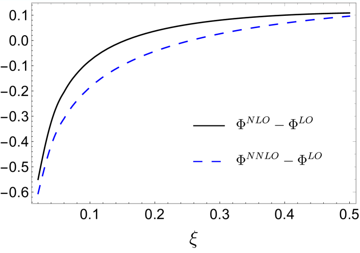
The results for the NNLO vs. NLO calculation of the $\pi\gamma^{\ast}\gamma$ form factor for the two models of the pion LCDA in Eq. (16) are shown in Fig. 3. In this calculation we set $\mu=Q$ and use the evolution equations both at NLO and NNLO Braun et al. (2017), to calculate the pion LCDA (16) at this scale. It is seen that the model dependence is comparable in size with the projected accuracy of the Belle II measurements. The NNLO correction is about a half of the model difference and has to be taken into account. We conclude that the NNLO accuracy is mandatory to constrain the pion LCDA from the analysis of theory predictions with the expected data. This, in turn, will have important consequences on the accuracy of QCD predictions in B-decays and other hard processes with energetic pions in the final state.

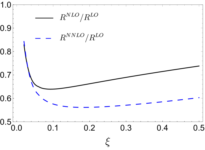
As already mentioned, the same CF enters the NNLO calculation of the contribution of the axial-vector GPD to DVCS. The DVCS amplitude (3) is a complex-valued function. Following Kumericki et al. (2008), we show in Fig. 4 the size of the NNLO two-loop correction for the absolute value and the phase difference of the corresponding Compton form factor at $Q^{2}=\mu^{2}=4\,\mathrm{GeV}^{2}$,

$$\widetilde{\mathcal{H}}(\xi)=R(\xi)\,e^{i\Phi(\xi)},$$ (21)

for the simplest ansatz for the GPD $\widetilde{H}$, see Eq. (3.330) in Belitsky and Radyushkin (2005), normalized in the forward limit to the polarized quark density $f(\beta)\sim\beta^{1/2}(1-\beta)^{4}$. The results are qualitatively very similar to the vector amplitude considered in Ref. Braun et al. (2020): The two-loop correction is large for the absolute value of the Compton form factor and small for the phase. A more detailed study including the scale dependence is premature at this time, as the axial-vector GPD is practically unknown. This task will become important in the future to analyze the forthcoming JLAB-12 and, later, EIC data.

Figure 4: The axial-vector Compton form factor $\mathcal{H}(\xi)$ in Eq. (21), calculated to NNLO and NLO accuracy. Shown are the ratios for the absolute values (top panel) and the phase differences (bottom panel), both with respect to the tree-level.

In summary, we have used innovative computational approaches based on conformal symmetry to advance the theoretical predictions for hard exclusive reactions to NNLO in QCD, which is the level of accuracy required by the precision of experimental data. We expect our results to have a broad range of applications in the analyses of data from current and future high-intensity, medium energy experiments.

Acknowledgments:    This study was supported by DFG Research Unit FOR 2926, Grant No. 40824754, DFG grants MO 1801/4-1, KN 365/13-1, and RSF project No. 19-11-00131. The authors are grateful to Yao Ji for communication on an independent calculation of the same CF by another method. We thank Sadaharu Uehara for providing us with the estimates for the expected accuracy of the Belle II experiment. Our special thanks are due to A.V. Pimikov for pointing out a misprint in the ancillary file.

Note Added:   Our result for the CF in Eq. (8)–(10) agrees with an independent calculation of the same CF using a different technique Gao et al. (2021), cf. Eqs. (26)–(29). It is easy to check that the analytic expressions in this work and in Gao et al. (2021) coincide identically.

References

- Aubert et al. (2009) B. Aubert et al. (BaBar), Phys. Rev. D 80, 052002 (2009), eprint 0905.4778.
- Uehara et al. (2012) S. Uehara et al. (Belle), Phys. Rev. D 86, 092007 (2012), eprint 1205.3249.
- Altmannshofer et al. (2019) W. Altmannshofer et al. (Belle-II), PTEP 2019, 123C01 (2019), [Erratum: PTEP 2020, 029201 (2020)], eprint 1808.10567.
- Dudek et al. (2012) J. Dudek et al., Eur. Phys. J. A48, 187 (2012), eprint 1208.1244.
- Akhunzyanov et al. (2019) R. Akhunzyanov et al. (COMPASS), Phys. Lett. B 793, 188 (2019), eprint 1802.02739.
- Accardi et al. (2016) A. Accardi et al., Eur. Phys. J. A52, 268 (2016), eprint 1212.1701.
- Abdul Khalek et al. (2021) R. Abdul Khalek et al. (2021), eprint 2103.05419.
- Gutierrez-Reyes et al. (2018) D. Gutierrez-Reyes, I. Scimemi, and A. Vladimirov, JHEP 07, 172 (2018), eprint 1805.07243.
- Braun et al. (2017) V. M. Braun, A. N. Manashov, S. Moch, and M. Strohmaier, JHEP 06, 037 (2017), eprint 1703.09532.
- Lepage and Brodsky (1979) G. P. Lepage and S. J. Brodsky, Phys. Lett. B 87, 359 (1979).
- Lepage and Brodsky (1980) G. P. Lepage and S. J. Brodsky, Phys. Rev. D 22, 2157 (1980).
- Diehl (2003) M. Diehl, Phys. Rept. 388, 41 (2003), eprint hep-ph/0307382.
- Belitsky and Radyushkin (2005) A. V. Belitsky and A. V. Radyushkin, Phys. Rept. 418, 1 (2005), eprint hep-ph/0504030.
- del Aguila and Chase (1981) F. del Aguila and M. K. Chase, Nucl. Phys. B 193, 517 (1981).
- Braaten (1983) E. Braaten, Phys. Rev. D 28, 524 (1983).
- Kadantseva et al. (1986) E. P. Kadantseva, S. V. Mikhailov, and A. V. Radyushkin, Yad. Fiz. 44, 507 (1986).
- Remiddi and Vermaseren (2000) E. Remiddi and J. A. M. Vermaseren, Int. J. Mod. Phys. A15, 725 (2000), eprint hep-ph/9905237.
- Melic et al. (2002) B. Melic, B. Nizic, and K. Passek, Phys. Rev. D 65, 053020 (2002), eprint hep-ph/0107295.
- Zijlstra and van Neerven (1994) E. B. Zijlstra and W. L. van Neerven, Nucl. Phys. B 417, 61 (1994), [Errata: Nucl.Phys.B 426, 245 (1994); 501, 599–599 (1997); 773, 105–106 (2007)].
- Moch and Vermaseren (2000) S. Moch and J. A. M. Vermaseren, Nucl. Phys. B 573, 853 (2000), eprint hep-ph/9912355.
- Melic et al. (2003) B. Melic, D. Müller, and K. Passek-Kumericki, Phys. Rev. D 68, 014013 (2003), eprint hep-ph/0212346.
- Braun et al. (2020) V. M. Braun, A. N. Manashov, S. Moch, and J. Schoenleber, JHEP 09, 117 (2020), eprint 2007.06348.
- Braun et al. (2021) V. M. Braun, A. N. Manashov, S. Moch, and M. Strohmaier (2021), eprint 2101.01471.
- Larin (1993) S. A. Larin, Phys. Lett. B 303, 113 (1993), eprint hep-ph/9302240.
- Braun et al. (2016) V. M. Braun, A. N. Manashov, S. Moch, and M. Strohmaier, JHEP 03, 142 (2016), eprint 1601.05937.
- Vermaseren (1999) J. Vermaseren, Int. J. Mod. Phys. A 14, 2037 (1999), eprint hep-ph/9806280.
- Ablinger (2009) J. Ablinger, Ph.D. thesis, Linz U. (2009), eprint 1011.1176.
- Ablinger (2014) J. Ablinger, PoS LL2014, 019 (2014), eprint 1407.6180.
- Basso and Korchemsky (2007) B. Basso and G. P. Korchemsky, Nucl. Phys. B775, 1 (2007), eprint hep-th/0612247.
- Alday et al. (2015) L. F. Alday, A. Bissi, and T. Lukowski, JHEP 11, 101 (2015), eprint 1502.07707.
- Panzer (2015) E. Panzer, Comput. Phys. Commun. 188, 148 (2015), eprint 1403.3385.
- Bali et al. (2019) G. S. Bali et al. (RQCD), JHEP 08, 065 (2019), [Addendum: JHEP 11, 037 (2020)], eprint 1903.08038.
- Gronberg et al. (1998) J. Gronberg et al. (CLEO), Phys. Rev. D 57, 33 (1998), eprint hep-ex/9707031.
- Kumericki et al. (2008) K. Kumericki, D. Müller, and K. Passek-Kumericki, Nucl. Phys. B794, 244 (2008), eprint hep-ph/0703179.
- Gao et al. (2021) J. Gao, T. Huber, Y. Ji, and Y.-M. Wang (2021), eprint 2106.01390.