Gauss-Seidel Method with Oblique Direction

Abstract

In this paper, a Gauss-Seidel method with oblique direction (GSO) is proposed for finding the least-squares solution to a system of linear equations, where the coefficient matrix may be full rank or rank deficient and the system is overdetermined or underdetermined. Through this method, the number of iteration steps and running time can be reduced to a greater extent to find the least-squares solution, especially when the columns of matrix A are close to linear correlation. It is theoretically proved that GSO method converges to the least-squares solution. At the same time, a randomized version–randomized Gauss-Seidel method with oblique direction (RGSO) is established, and its convergence is proved. Theoretical proof and numerical results show that the GSO method and the RGSO method are more efficient than the coordinate descent (CD) method and the randomized coordinate descent (RCD) method.

Key words: linear least-squares problem, oblique direction, coordinate descent method, randomization, convergence property.

1 Introduction

Consider a linear least-squares problem

$$\mathop{arg\min}\limits_{x\in R^{n}}\|Ax-b\|^{2},$$ (1)

where $b\in R^{m}$ is a real $m$ dimensional vector, and the columns of coefficient matrix $A\in R^{m\times n}$ are non-zero, which doesn’t lose the generality of matrix $A$. Here and in the sequel, $\|\cdot\|$ indicates the Euclidean norm of a vector. When $A$ is full column rank, $(\ref{e1})$ has a unique solution $x^{*}=A^{{\dagger}}b=(A^{T}A)^{-1}A^{T}b$, where $A^{{\dagger}}$ and $A^{T}$ are the Moore-Penrose pseudoinverse [3] and the transpose of $A$, respectively. One of the iteration methods that can be used to solve $(\ref{e1})$ economically and effectively is the coordinate descent (CD) method [10], which is also obtained by applying the classical Gauss-Seidel iteration method to the following normal equation (see [22])

$$A^{T}Ax=A^{T}b.$$ (2)

In solving $(\ref{e1})$, the CD method has a long history of development, and is widely used in various fields, such as machine learning [7], biological feature selection [6], tomography [5, 29], and so on. Inspired by the randomized coordinate descent (RCD) method proposed by Leventhal and Lewis [10] and its linear convergence rate analyzed theoretically [12], a lot of related work such as the randomized block versions [11, 13, 21] and greedy randomized versions of the CD method [1, 30] have been developed and studied. For more information about a variety of randomized versions of the coordinate descent method, see [17, 23, 28] and the references therein. These methods mentioned above are based on the CD method, and can be extended to Kaczmarz-type methods. The recent work of Kaczmarz-type method can be referred to [26, 25, 15, 16, 2, 24, 20]. Inspired by the above work, We propose a new descent direction based on the construction idea of the CD method, which is formed by the weighting of two coordinate vectors. Based on this, we propose a Gauss-Seidel method with oblique direction (GSO) and construct the randomized version–randomized Gauss-Seidel method with oblique direction (RGSO), and analyze the convergence properties of the two methods.

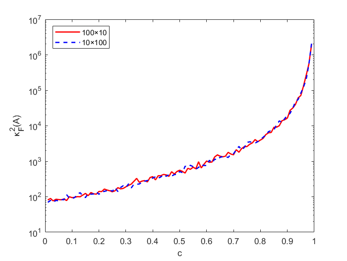
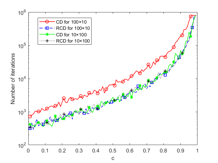
Regarding our proposed methods–the GSO method and the RGSO method, we emphasize the efficiency when the columns of matrix $A$ are close to linear correlation. In [14], it is mentioned that when the rows of matrix $A$ are close to linear correlation, the convergence speed of the K method and the randomized Kaczmarz method [27] decrease significantly. Inspired by the above phenomena, we experimented the convergence performance of the CD method and the RCD method when the columns of matrix A are close to linear correlation and it is found through experiments that the theoretical convergence speed and experimental convergence speed of the CD method and the the RCD method will be greatly reduced. The exponential convergence in expectation of the RCD method is as follows:

$$E_{k}\delta(x^{(k+1)})\leq\left(1-\frac{1}{\kappa_{F}^{2}(A)}\right)\delta(x^{(k)}),$$ (3)

where $\delta(x)=F(x)-minF$, $F(x)=\|Ax-b\|^{2}$. Here and in the sequel, $||A||_{2}=\mathop{max}\limits_{\|x\|=1}||Ax||$, $||A||_{F}$, $\kappa_{F}(A)=||A||_{F}\cdot||A^{\dagger}||_{2}$ are used to denote Euclidean norm, Frobenius norm and the scaled condition number of the matrix $A$, respectively. The subgraph (a) in Figure 1 shows that when the column of matrix $A$ is closer to the linear correlation, $\kappa_{F}^{2}(A)$ will become larger, which further reduce the convergence rate of the RCD method. The subgraph (b) in Figure 1 illustrates the sensitivity of the CD method and the RCD method to linear correlation column of $A$. This further illustrates the necessity of solving this type of problem, and the GSO method and the RGSO method we proposed can be used effectively to solve that one. For the initial data setting, explanation of the experiment in Figure 1 and the experiment on this type of matrix, please refer to Section 4 in this paper.

Figure 1: Matrix $A$ is generated by the $rand$ function in the interval $[c,1]$. (a): $\kappa_{F}^{2}(A)$ of matrix $A$ changes with $c$. (b): When the system is consistent, the number of iterations for the CD method and the RCD method to converge with the change of c, where the maximum number of iterations is limited to 800,000.

In this paper, $\langle\cdot\rangle$ stands for the scalar product, and we indicate by $e_{i}$ the column vector with 1 at the ith position and 0 elsewhere. In addition, for a given matrix $G=(g_{ij})\in R^{m\times n}$, $g_{i}^{T}$, $G_{j}$ and $\sigma_{min}(G)$, are used to denote its ith row, jth column and the smallest nonzero singular value of $G$ respectively. Given a symmetric positive semidefinite matrix $G\in R^{n\times n}$, for any vector $x\in R^{n}$ we define the corresponding seminorm as $||x||_{G}=\sqrt{x^{T}Gx}$. Let $E_{k}$ denote the expected value conditonal on the first k iterations, that is,

$$E_{k}[\cdot]=E[\cdot|j_{0},j_{1},...,j_{k-1}],$$

where $j_{s}(s=0,1,...,k-1)$ is the column chosen at the sth iteration.

The organization of this paper is as follows. In Section 2, we introduce the CD method and its construction idea. In Section 3, we propose the GSO method naturally and get its randomized version–RGSO method, and prove the convergence of the two methods. In Section 4, some numerical examples are provided to illustrate the effectiveness of our new methods. Finally, some brief concluding remarks are described in Section 5.

2 Coordinate Descent Method

Consider a linear system

$$\tilde{A}x=b,$$ (4)

where the coefficient matrix $\tilde{A}\in R^{n\times n}$ is a positive-definite matrix, and $b\in R^{n}$ is a real m dimensional vector. $\tilde{x}^{*}=\tilde{A}^{-1}b$ is the unique solution of $(\ref{e4})$. In this case, solving $(\ref{e4})$ is equivalent to the following strict convex quadratic minimization problem

$$f(x)=\frac{1}{2}x^{T}\tilde{A}x-b^{T}x.$$

From [10], the next iteration point $x^{(k+1)}$ is the solution to $\mathop{min}\limits_{\begin{subarray}{c}t\in R\end{subarray}}f(x^{(k)}+td)$, i.e.

$$x^{(k+1)}=x^{(k)}+\frac{(b-\tilde{A}x^{(k)})^{T}d}{d^{T}\tilde{A}d}d,$$ (5)

where $d$ is a nonzero direction, and $x^{(k)}$ is a current iteration point. It is easily proved that

$$f(x^{(k+1)})-f(\tilde{x}^{*})=\frac{1}{2}\|x^{(k+1)}-\tilde{x}^{*}\|^{2}_{\tilde{A}}=\frac{1}{2}\|x^{(k)}-\tilde{x}^{*}\|^{2}_{\tilde{A}}-\frac{((b-\tilde{A}x^{(k)})^{T}d)^{2}}{2d^{T}\tilde{A}d}.$$ (6)

One natural choice of a set of easily computable search directions is to choose $d$ by successively cycling through the set of canonical unit vectors $\left\{e_{1},...,e_{n}\right\}$, where $e_{i}\in R^{n},i=1,\cdots,n$. When $A\in R^{m\times n}$ is full column rank, we can apply $(\ref{e2})$ to $(\ref{e5})$ to get:

$$x^{(k+1)}=x^{(k)}+\frac{\langle r^{(k)},A_{i}\rangle}{||A_{i}||^{2}}e_{i},$$

where $i=mod(k,n)+1$. This is the iterative formula of CD method, also known as Gauss-Seidel method. This method is linearly convergent but with a rate not easily expressible in terms of typical matrix quantities. See [4, 8, 19]. The CD method can only ensure that one entry of $A^{T}r$ is 0 in each iteration, i.e. $A_{i}^{T}r^{(k)}=0\ \ (i=mod(k,n)+1)$. In the next chapter, we propose a new oblique direction $d$ for $(\ref{e5})$, which is the weight of the two coordinate vectors, and use the same idea to get a new method– the GSO method. The GSO method can ensure that the two entries of $A^{T}r$ are 0 in each iteration, thereby accelerating accelerating the convergence.

Remark 1. When $\tilde{A}$ is positive semidefinite matrix, $(\ref{e4})$ may not have a unique solution, replace $\tilde{x}^{*}$ with any least-squares solution, $(\ref{e5})$, $(\ref{e6})$ still hold, if $d^{T}\tilde{A}d\neq 0$.

Remark 2.  The Kaczmarz method can be regarded as a special case of $(\ref{e5})$ under a different regularizing linear system

$$AA^{T}y=b,\ \ x=A^{T}y,$$ (7)

when $d$ is selected cyclically through the set of canonical unit vectors $\left\{e_{1},...,e_{m}\right\}$, where $e_{i}\in R^{m}$, $i=1,2,\cdots,m$.

3 Gauss-Seidel Method with Oblique Direction and its Randomized Version

3.1 Gauss-Seidel Method with Oblique Direction

We propose a similar $d$, that is $d=e_{i_{k+1}}-\frac{\langle A_{i_{k+1}},A_{i_{k}}\rangle}{||A_{i_{k}}||^{2}}e_{i_{k}}$, where $e_{i}\in R^{n}$, $i=1,2,\cdots,n$. Using $(\ref{e2})$ and $(\ref{e5})$, we get

$$x^{(k+1)} =x^{(k)}+\frac{(A^{T}b-A^{T}Ax^{(k)})^{T}(e_{i_{k+1}}-\frac{\langle A_{i_{k+1}},A_{i_{k}}\rangle}{||A_{i_{k}}||^{2}}e_{i_{k}})}{\left\|A(e_{i_{k+1}}-\frac{\langle A_{i_{k+1}},A_{i_{k}}\rangle}{||A_{i_{k}}||^{2}}e_{i_{k}})\right\|^{2}}(e_{i_{k+1}}-\frac{\langle A_{i_{k+1}},A_{i_{k}}\rangle}{||A_{i_{k}}||^{2}}e_{i_{k}})$$

$$=x^{(k)}+\frac{A_{i_{k+1}}^{T}r^{(k)}-\frac{\langle A_{i_{k+1}},A_{i_{k}}\rangle}{||A_{i_{k}}||^{2}}A_{i_{k}}^{T}r^{(k)}}{||A_{i_{k+1}}||^{2}-\frac{\langle A_{i_{k+1}},A_{i_{k}}\rangle^{2}}{||A_{i_{k}}||^{2}}}(e_{i_{k+1}}-\frac{\langle A_{i_{k+1}},A_{i_{k}}\rangle}{||A_{i_{k}}||^{2}}e_{i_{k}}).$$ (8)

Now we prove that $A_{i_{k}}^{T}r^{(k)}=0.$

$$A_{i_{k}}^{T}r^{(k)} =\langle A_{i_{k}},b-Ax^{(k)}\rangle$$

$$=\langle A_{i_{k}},r^{(k-1)}\rangle-\langle A_{i_{k}},r^{(k-1)}\rangle+\frac{\langle A_{i_{k}},A_{i_{k-1}}\rangle}{||A_{i_{k-1}}||^{2}}A_{i_{k-1}}^{T}r^{(k-1)}$$

$$=\frac{\langle A_{i_{k}},A_{i_{k-1}}\rangle}{||A_{i_{k-1}}||^{2}}A_{i_{k-1}}^{T}r^{(k-1)},\ \ k=2,3,...$$

We only need to guarantee $A_{i_{1}}^{T}r^{(1)}=0$, so we need to take the simplest coordinate descent projection as the first step. $(\ref{e8})$ becomes

$$x^{(k+1)}=x^{(k)}+\frac{A_{i_{k+1}}^{T}r^{(k)}}{||A_{i_{k+1}}||^{2}-\frac{\langle A_{i_{k+1}},A_{i_{k}}\rangle^{2}}{||A_{i_{k}}||^{2}}}(e_{i_{k+1}}-\frac{\langle A_{i_{k+1}},A_{i_{k}}\rangle}{||A_{i_{k}}||^{2}}e_{i_{k}}).$$

The algorithm is described in Algorithm 3.1. Without losing generality, we assume that all columns of $A$ are not zero vectors.

  Algorithm 1 Gauss-Seidel method with Oblique Projection (GSO)

 

1:$A\in R^{m\times n}$, $b\in R^{m}$, $x^{(0)}\in R^{n}$, $K$, $\varepsilon>0$

2:For $i=1:n$, $N(i)=\|A_{i}\|^{2}$

3:Compute $r^{(0)}=b-Ax^{(0)}$, $\alpha_{0}=\frac{\langle A_{1},r^{(0)}\rangle}{N(1)}$, $x^{(1)}=x^{(0)}+\alpha_{0}e_{1}$, $r^{(1)}=r^{(0)}-\alpha_{0}A_{1}$, and set $i_{k+1}=1$

4:for $k=1,2,\cdots,K-1$ do

5:     Set $i_{k}=i_{k+1}$ and choose a new $i_{k+1}$: $i_{k+1}=mod(k,n)+1$

6:     Compute $G_{i_{k}}=\langle A_{i_{k}},A_{i_{k+1}}\rangle$  and $g_{i_{k}}=N(i_{k+1})-\frac{G_{i_{k}}}{N(i_{k})}G_{i_{k}}$

7:     if $g_{i_{k}}>\varepsilon$ then

8:         Compute $\alpha_{k}=\frac{\langle A_{i_{k+1}},r^{(k)}\rangle}{g_{i_{k}}}$  and $\beta_{k}=-\frac{G(i_{k})}{N(i_{k})}\alpha_{k}$

9:         Compute $x^{(k+1)}=x^{(k)}+\alpha_{k}e_{i_{k+1}}+\beta_{k}e_{i_{k}}$, and $r^{(k+1)}=r^{(k)}-\alpha_{k}A_{i_{k+1}}-\beta_{k}A_{i_{k}}$

10:     end if

11:end for

12:Output $x^{(K)}$

 

It’s easy to get

$$A_{i_{k-1}}^{T}r^{(k)} =A_{i_{k-1}}^{T}(r^{(k-1)}-\alpha_{k-1}A_{i_{k}}-\beta_{k-1}A_{i_{k-1}})$$

$$=A_{i_{k-1}}^{T}(r^{(k-1)}-\frac{\langle A_{i_{k}},r^{(k-1)}\rangle}{g_{i_{k-1}}}A_{i_{k}}+\frac{\langle A_{i_{k-1}},A_{i_{k}}\rangle\langle A_{i_{k}},r^{(k-1)}\rangle}{||A_{i_{k-1}}||^{2}g_{i_{k}}}A_{i_{k-1}})$$

$$=0.\ \ k=2,3,\cdots$$

The last equality holds due to $A_{i_{k}}^{T}r^{(k)}=0,k=1,2,\cdots$. Before giving the proof of the convergence of the GSO method, we redefine the iteration point. For $x^{(0)}\in R^{n}$ as initial approximation, we define $x^{(0,0)}$, $x^{(0,1)},...,x^{(0,n)}\in R^{n}$ by

$$\left\{\begin{array}[]{lr}x^{(0,0)}=x^{(0)}+\frac{A_{1}^{T}(b-Ax^{(0)})}{||A_{1}||^{2}}e_{1},&\\ x^{(0,1)}=x^{(0,0)}+\frac{A_{2}^{T}(b-Ax^{(0,0)})}{||A_{2}||^{2}-\frac{\langle A_{2},A_{1}\rangle^{2}}{||A_{1}||^{2}}}(e_{2}-\frac{\langle A_{2},A_{1}\rangle}{||A_{1}||^{2}}e_{1}),&\\ x^{(0,2)}=x^{(0,1)}+\frac{A_{3}^{T}(b-Ax^{(0,1)})}{||A_{3}||^{2}-\frac{\langle A_{3},A_{2}\rangle^{2}}{||A_{2}||^{2}}}(e_{3}-\frac{\langle A_{3},A_{2}\rangle}{||A_{2}||^{2}}e_{2}),&\\ \cdots\cdots\cdots\cdots\cdots\cdots\cdots\cdots\cdots&\\ x^{(0,n-1)}=x^{(0,n-2)}+\frac{A_{n}^{T}(b-Ax^{(0,n-2)})}{||A_{n}||^{2}-\frac{\langle A_{n},A_{n-1}\rangle^{2}}{||A_{n-1}||^{2}}}(e_{n}-\frac{\langle A_{n},A_{n-1}\rangle}{||A_{n-1}||^{2}}e_{n-1}),&\\ x^{(0,n)}=x^{(0,n-1)}+\frac{A_{1}^{T}(b-Ax^{(0,n-1)})}{||A_{1}||^{2}-\frac{\langle A_{1},A_{n}\rangle^{2}}{||A_{n}||^{2}}}(e_{1}-\frac{\langle A_{1},A_{n}\rangle}{||A_{n}||^{2}}e_{n}).&\\ \end{array}\right.$$ (9)

For convenience, denote $A_{n+1}=A_{1},$ $b_{n+1}=b_{1}$. When the iteration point $x^{(p,n)}$ ${\forall p\geq 0}$ is given, the iteration points are obtained continuously by the following formula

$$\left\{\begin{array}[]{lr}for\;\;i=1:n&\\ x^{(p+1,i)}=x^{(p+1,i-1)}+\frac{A_{i+1}^{T}(b-Ax^{(p+1,i-1)})}{||A_{i+1}||^{2}-\frac{\langle A_{i+1},A_{i}\rangle^{2}}{||A_{i}||^{2}}}(e_{i+1}-\frac{\langle A_{i+1},A_{i}\rangle}{||A_{i}||^{2}}e_{i}),\\ end\end{array}\right.$$ (10)

where $x^{(p+1,0)}=x^{(p,n)}$. Then, we can easily obtain that $x^{(k+1)}=x^{(p,i)}$, and $A_{i_{k}}^{T}r^{(k)}=A_{i+1}^{T}r^{(p,i)}=0$, if $k=p\cdot n+i,0\leq i<n.$

The convergence of the GSO is provided as follows.

Theorem 1.

Consider $(\ref{e1})$, where the coefficient $A\in R^{m\times n}$, $b\in R^{m}$ is a given vector, and $\tilde{x}$ is any least-squares solution of $(\ref{e1})$. Let $x^{(0)}\in R^{n}$ be an arbitrary initial approximation, then the sequence $\{Ax^{(k)}\}_{k=1}^{\infty}$ generated by the GSO algorithm is convergent , and satisfy the following equation:

$$\lim_{k\rightarrow\infty}\|x^{(k)}-\tilde{x}\|_{A^{T}A}=0.$$ (11)

Proof.

According to $(\ref{e3.2})$-$(\ref{e3.3})$ we obtain the sequence of approximations (from top to bottom and left to right, and by also using the notational convention $x^{(p+1,0)}=x^{(p,n)}$).

$$\left\{\begin{array}[]{lr}x^{(0)},x^{(0,0)}&\\ x^{(0,1)},x^{(0,2)},\cdots,x^{(0,n)}=x^{(1,0)}&\\ x^{(1,1)},x^{(1,2)},\cdots,x^{(1,n)}=x^{(2,0)}&\\ \cdots\cdots\cdots\cdots\cdots\cdots\cdots\cdots\cdots&\\ x^{(p,1)},x^{(p,2)},\cdots,x^{(p,n)}=x^{(p+1,0)}&\\ \cdots\cdots\cdots\cdots\cdots\cdots\cdots\cdots\cdots\end{array}\right.$$

Apply $(\ref{e2})$ to $(\ref{e6})$,we get

$$||x^{(p,i+1)}-\tilde{x}||^{2}_{A^{T}A}=||x^{(p,i)}-\tilde{x}||^{2}_{A^{T}A}-\frac{((A^{T}b-A^{T}Ax^{(p,i)})^{T}d)^{2}}{d^{T}A^{T}Ad},$$ (12)

where $d=e_{i+2}-\frac{\langle A_{i+2},A_{i+1}\rangle}{||A_{i+1}||^{2}}e_{i+1}$, $e_{i}\in R^{n},i=1,\cdots,n.$ Obviously, the sequence $\{\|x^{(p,i)}-x^{*}\|_{A^{T}A}\}_{p=0,i=0}^{\infty,n-1}$, i.e. $\{\|x^{(k+1)}-x^{*}\|_{A^{T}A}\}_{k=1}^{\infty}$ is a monotonically decreasing sequence with lower bounds. There exists a $\alpha\geq 0$ such that

$$\lim_{p\rightarrow\infty}\|x^{(p,i)}-\tilde{x}\|_{A^{T}A}=\alpha\geq 0,\ \ \forall\ i=0,1,\cdots,n-1.$$ (13)

Thus, take the limit of $p$ on both sides of $(\ref{e3.5})$, and because $i$ was arbitrary we apply $A_{i_{k+1}}^{T}r^{(p,i)}=0$, and get

$$\lim_{p\rightarrow\infty}A_{i+2}^{T}r^{(p,i)}=0,\ \ \forall\ i=0,1,\cdots,n-1.$$ (14)

The residuals satisfy

$$r^{(p,i)}=r^{(p,i)}-\frac{\langle A_{i+2},r^{(p,i)}\rangle}{||A_{i+2}||^{2}-\frac{\langle A_{i+2},A_{i+1}\rangle^{2}}{||A_{i+1}||^{2}}}\left(A_{i+2}-\frac{\langle A_{i+2},A_{i+1}\rangle}{||A_{i+1}||^{2}}A_{i+1}\right).$$

Taking the limit of p on both sides of the above equation, we get

$$\lim_{p\rightarrow\infty}r^{(p,i+1)}=\lim_{p\rightarrow\infty}r^{(p,i)},\ \ \forall\ i=0,1,\cdots,n-1.$$

Using the above equation and $(\ref{e3.7})$, we can easily deduce that

$$\lim_{p\rightarrow\infty}A^{T}r^{(p,i)}=0,\ \ \forall\ i=0,1,\cdots,n-1.$$ (15)

Because the sequence $\{\|x^{(p,i)}-\tilde{x}\|_{A^{T}A}\}_{p=0,i=0}^{\infty,n-1}$ is bounded, we obtain

$$\|x^{(p,i)}\|_{A^{T}A}\leq\|\tilde{x}\|_{A^{T}A}+\|x^{(p,i)}-\tilde{x}\|_{A^{T}A}\leq\|\tilde{x}\|_{A^{T}A}+\|x^{(0,1)}-\tilde{x}\|_{A^{T}A},\,\,\forall p\geq 0.$$ (16)

According to $(\ref{e3.9})$ we get that the sequence $\{Ax^{(p,0)}\}_{p=0}^{\infty}$ is bounded, thus there exists a convergent subsequence $\{Ax^{(p_{j},0)}\}_{j=1}^{\infty}$, let’s denote it as

$$\lim_{j\rightarrow\infty}Ax^{(p_{j},0)}=\hat{b}.$$ (17)

From $(\ref{e3.2})$-$(\ref{e3.3})$, we get

$$x^{(p_{j},1)}=x^{(p_{j},0)}-\frac{A^{T}_{2}(b-Ax^{(p_{j},0)})}{||A_{2}||^{2}-\frac{\langle A_{2},A_{1}\rangle^{2}}{||A_{1}||^{2}}}\left(e_{2}-\frac{\langle A_{2},A_{1}\rangle}{||A_{1}||^{2}}e_{1}\right),\,\,\,\forall\ j>0.$$

By multiplying the both sides of the above equation left by matrix $A$ and using $(\ref{e3.7})$, we can get that

$$\lim_{j\rightarrow\infty}Ax^{(p_{j},1)}=\hat{b}.$$

With the same way we obtain

$$\lim_{j\rightarrow\infty}Ax^{(p_{j},i)}=\hat{b},\,\,\,\,\forall\ i=0,1,\cdots,n-1.$$

Then, from $(\ref{e3.8})$ we get for any $i=1,\cdots,n-1$,

$$\lim_{j\rightarrow\infty}A^{T}r^{(p_{j},i)}=A^{T}(b-\hat{b})=0.$$

From $(\ref{e3.6})$ and the above equation, we get

$$\lim_{j\rightarrow\infty}\|x^{(p_{j},i)}-\tilde{x}\|_{A^{T}A}=\alpha=0,\ \ \ \forall\ i=0,1,\cdots,n-1$$

Hence,

$$\lim_{p\rightarrow\infty}\|x^{(p,i)}-\tilde{x}\|_{A^{T}A}=0,\ \ \ \forall\ i=0,1,\cdots,n-1$$

then $(\ref{e3.4})$ holds. ∎

Remark 3.  When $g_{i_{k}}=0$, $A_{i_{k+1}}$ is parallel to $A_{i_{k}}$, i.e. $\exists\lambda>0$, s.t. $A_{i_{k}}=\lambda A_{i_{k+1}}$. According to the above derivation, the GSO method is used to solve (1.2) which is consistent, so the following equation holds:

$$A_{i_{k}}^{T}b=\lambda A_{i_{k+1}}^{T}b,$$

which means for $(\ref{e2})$ the $i_{k}$th equation: $\langle A_{i_{k}},Ax\rangle=A^{T}_{i_{k}}b$, and the $i_{k+1}$th equation: $\langle A_{i_{k+1}},Ax\rangle=A^{T}_{i_{k+1}}b$ are coincident, and we can skip this step without affecting the final calculation to obtain the least-squares solution. When $g_{i_{k}}$ is too small, it is easy to produce large errors in the process of numerical operation, and we can regard it as the same situation as $g_{i_{k}}=0$ and skip this step.

Remark 4.  By the GSO method, we have: $||x^{(k+1)}-\tilde{x}||^{2}_{A^{T}A}=||x^{(k)}-\tilde{x}||^{2}_{A^{T}A}-\frac{(A_{i_{k+1}}^{T}r^{k})^{2}}{g_{i_{k}}}$, where $g_{i_{k}}=\|A_{i_{k+1}}\|^{2}-\frac{\langle A_{i_{k+1}},A_{i_{k}}\rangle^{2}}{\|A_{i_{k}}\|^{2}}$. But the CD method holds: $||x^{(k+1)}-\tilde{x}||^{2}_{A^{T}A}=||x^{(k)}-\tilde{x}||^{2}_{A^{T}A}-\frac{(A_{i_{k+1}}^{T}r^{k})^{2}}{||A_{i_{k+1}}||^{2}}$. So the GSO method is faster than the CD method unless $\langle A_{i_{k}},A_{i_{k+1}}\rangle=0$. When $\langle A_{i_{k}},A_{i_{k+1}}\rangle=0$, the convergence rate of the GSO method is the same as that of the CD method. This means that when the coefficient matrix $A$ is a column orthogonal matrix, the GSO method degenerates to the CD method.

Remark 5.   The GSO method needs $8m+5$ floating-point operations per step, and the CD method needs $4m+1$ floating-point operations per step.

Remark 6.  When the matrix $A$ is full column rank, let $x^{*}$ be the unique least-squares solution of $(\ref{e1})$, the sequence $\{x^{(k)}\}_{k=1}^{\infty}$ generated by the GSO method holds: $\lim\limits_{k\rightarrow\infty}\|x^{(k)}-x^{*}\|_{A^{T}A}=0$, that is, $\lim\limits_{k\rightarrow\infty}\|A(x^{(k)}-x^{*})\|^{2}=0$. Therefore,

$$\lim_{k\rightarrow\infty}\|x^{(k)}-x^{*}\|^{2}=0.$$

Example 1.

Consider the following systems of linear equations

$$\left\{\begin{array}[]{rrr}5x_{1}+45x_{2}&=&50,\\ 9x_{1}+80x_{2}&=&89,\end{array}\right.$$ (18)

$$\left\{\begin{array}[]{rrr}x_{1}+11x_{2}&=&12,\\ -2x_{1}-21x_{2}&=&-23,\\ 3x_{1}+32x_{2}&=&35\end{array}\right.$$ (19)

and

$$\left\{\begin{array}[]{rrr}x_{1}+9x_{2}&=&0,\\ 4x_{1}+36x_{2}&=&42.5,\\ 13x_{1}+118x_{2}&=&131,\end{array}\right.$$ (20)

$(\ref{e3.11})$ is square and consistent, $(\ref{e3.12})$ is overdetermined and consistent, and $(\ref{e3.13})$ is overdetermined and inconsistent. Vector $x^{*}=(1,1)^{T}$ is the unique solution to the above $(\ref{e3.11})$ and $(\ref{e3.12})$, is the unique least-squares solution to $(\ref{e3.13})$. It can be found that the column vectors of these systems are close to linearly correlated. Numerical experiments show that they take $650259$, $137317$, $3053153$ steps respectively for the CD method to be applied to the above systems to reach the relative solution error requirement $\frac{\|x^{(k)}-x^{*}\|^{2}}{\|x^{*}\|^{2}}\leq\frac{1}{2}\times 10^{-6}$, but the GSO method can find the objective solutions to the above three systems in one step.

3.2 Randomized Gauss-Seidel Method with Oblique Direction

If the columns whose residual entries are not 0 in algorithm 3.1 are selected uniformly and randomly, we get a randomized Gauss-seidel method with oblique direction (RGSO) and its convergence as follows.

  Algorithm 2 Randomized Gauss-Seidel Method with Oblique Direction (RGSO)

 

1:$A\in R^{m\times n}$, $b\in R^{m}$, $x^{(0)}\in R^{n}$, $K$, $\varepsilon>0$

2:For $i=1:n$, $N(i)=\|A_{i}\|^{2}$

3:Randomly select $i_{1}$, and compute $r^{(0)}=b-Ax^{(0)}$, $\alpha_{0}=\frac{\langle A_{i_{1}},r^{(0)}\rangle}{||A_{i_{1}}||^{2}}$, and $x^{(1)}=x^{(0)}+\alpha_{0}e_{i_{1}}$

4:Randomly select $i_{2}\neq i_{1}$, and compute $r^{(1)}=r^{(0)}-\alpha_{0}A_{i_{1}}$, $\alpha_{1}=\frac{\langle A_{i_{2}},r^{(1)}\rangle}{||A_{i_{2}}||^{2}-\frac{\langle A_{i_{1}},A_{i_{2}}\rangle^{2}}{||A_{i_{1}}||^{2}}}$, and $\beta_{1}=-\frac{\langle A_{i_{1}},A_{i_{2}}\rangle}{||A_{i_{1}}||^{2}}\alpha_{1}$

5:Compute $x^{(2)}=x^{(1)}+\alpha_{1}e_{i_{2}}+\beta_{1}e_{i_{1}}$,and $r^{(2)}=r^{(1)}-\alpha_{1}A_{i_{2}}-\beta_{1}A_{i_{1}}$

6:for $k=2,3,\cdots,K-1$ do

7:     Randomly select $i_{k+1}$ $(i_{k+1}\neq i_{k},i_{k-1})$

8:     Compute $G_{i_{k}}=\langle A_{i_{k}},A_{i_{k+1}}\rangle$  and $g_{i_{k}}=N(i_{k+1})-\frac{G_{i_{k}}}{N(i_{k})}G_{i_{k}}$

9:     if $g_{i_{k}}>\varepsilon$ then

10:         Compute $\alpha_{k}=\frac{\langle A_{i_{k+1}},r^{(k)}\rangle}{g_{i_{k}}}$  and $\beta_{k}=-\frac{G(i_{k})}{N(i_{k})}\alpha_{k}$

11:         Compute $x^{(k+1)}=x^{(k)}+\alpha_{k}e_{i_{k+1}}+\beta_{k}e_{i_{k}}$, and $r^{(k+1)}=r^{(k)}-\alpha_{k}A_{i_{k+1}}-\beta_{k}A_{i_{k}}$

12:     end if

13:end for

14:Output $x^{(K)}$

 

Lemma 1.

Consider $(\ref{e1})$, where the coefficient $A\in R^{m\times n}$ , $b\in R^{m}$ is a given vector, and $\tilde{x}$ is any solution to $(\ref{e1})$ , then we obtain the bound on the following expected conditional on the first $k$ $(k\geq 2)$ iteration of the RGSO

$$E_{k}\frac{(A_{i_{k+1}}^{T}r^{(k)})^{2}}{g_{i_{k}}}\geq\frac{1}{n-2}\frac{\sigma_{min}^{2}(A)||\tilde{x}-x^{(k)}||^{2}_{A^{T}A}}{||A||^{2}_{F}-\sigma_{min}^{2}(A)}.$$

Proof.

For the RGSO mthod, it is easy to get that $A_{i_{k}}^{T}r^{(k)}=0\ \ (k=1,2,\cdots)$ and $A_{i_{k-1}}^{T}r^{(k)}=0\ \ (k=2,3,\cdots)$ are still valid.

$$E_{k}\frac{(A_{i_{k+1}}^{T}r^{(k)})^{2}}{g_{i_{k}}} =\frac{1}{n-2}\sum\limits_{\begin{subarray}{c}s=1\\ s\not=i_{k},i_{k-1}\end{subarray}}^{n}\frac{(A_{s}^{T}r^{(k)})^{2}}{||A_{s}||^{2}-\frac{\langle A_{s},A_{i_{k}}\rangle^{2}}{||A_{i_{k}}||^{2}}}$$

$$\geq\frac{1}{n-2}\frac{\sum\limits_{\begin{subarray}{c}s=1,s\not=i_{k},i_{k-1}\end{subarray}}^{n}(A_{s}^{T}r^{(k)})^{2}}{\sum\limits_{\begin{subarray}{c}s=1\\ s\not=i_{k},i_{k-1}\end{subarray}}^{n}(||A_{s}||^{2}-\frac{\langle A_{s},A_{i_{k}}\rangle^{2}}{||A_{i_{k}}||^{2}})}\left(=\frac{1}{n-2}\frac{\sum\limits_{\begin{subarray}{c}s=1\end{subarray}}^{n}(A_{s}^{T}r^{(k)})^{2}}{\sum\limits_{\begin{subarray}{c}s=1\end{subarray}}^{n}(||A_{s}||^{2}-\frac{\langle A_{s},A_{i_{k}}\rangle^{2}}{||A_{i_{k}}||^{2}})}\right)$$

$$=\frac{1}{n-2}\frac{||A^{T}A(\tilde{x}-x^{(k)})||^{2}}{||A||^{2}_{F}-\frac{||A^{T}A_{i_{k}}||^{2}}{||A_{i_{k}}||^{2}}}$$

$$\geq\frac{1}{n-2}\frac{\sigma_{min}^{2}(A)||\tilde{x}-x^{(k)}||^{2}_{A^{T}A}}{||A||^{2}_{F}-\sigma_{min}^{2}(A)},\ \ k=2,3,...$$

The first inequality uses the conclusion of $\frac{|b_{1}|}{|a_{1}|}+\frac{|b_{2}|}{|a_{2}|}\geq\frac{|b_{1}|+|b_{2}|}{|a_{1}|+|a_{2}|}$ (if $|a_{1}|>0$, $|a_{2}|>0$), and the second one uses the conclusion of $\|A^{T}z\|_{2}^{2}\geq\sigma_{min}^{2}(A)\|z\|_{2}^{2}$, if $z\in R(A)$. ∎

Theorem 2.

Consider $(\ref{e1})$, where the coefficient $A\in R^{m\times n}$ , $b\in R^{m}$ is a given vector, and $\tilde{x}$ is any least-squares solution of $(\ref{e1})$. Let $x^{(0)}\in R^{n}$ be an arbitrary initial approximation, and define the least-squares residual and error by

$$F(x)=||Ax-b||^{2},$$

$$\delta(x)=F(x)-minF,$$

then the RGSO method is linearly convergent in expectation to a solution in $(\ref{e1})$.

For each iteration:$k=2,3,...$,

$$E_{k}\delta(x^{(k+1)})\leq\left(1-\frac{1}{(n-2)(k_{F}^{2}(A)-1)}\right)\delta(x^{(k)}).$$

In particular, if $A$ has full column rank, we have the equivalent property

$$E_{k}\left[\|x^{(k+1)}-x^{*}\|^{2}_{A^{T}A}\right]\leq\left(1-\frac{1}{(n-2)(k_{F}^{2}(A)-1)}\right)\|x^{(k)}-x^{*}\|^{2}_{A^{T}A},$$

where $x^{*}=A^{{\dagger}}b=(A^{T}A)^{-1}A^{T}b$ is the unique least-squares solution.

Proof.

It is easy to prove that

$$F(x)-F(\tilde{x})=||x-\tilde{x}||^{2}_{A^{T}A}=\delta(x).$$

Apply $(\ref{e2})$ to $(\ref{e6})$ with $d=e_{i_{k+1}}-\frac{\langle A_{i_{k+1}},A_{i_{k}}\rangle}{||A_{i_{k}}||^{2}}e_{i_{k}}$ and $A_{i_{k}}^{T}r_{k}=0,k=1,2,..$ ,we get that

$$F(x^{(k+1)})-F(\tilde{x}) =||x^{(k+1)}-\tilde{x}||^{2}_{A^{T}A}$$

$$=||x^{(k)}-\tilde{x}||^{2}_{A^{T}A}-\frac{(A^{T}_{i_{k+1}}r^{(k)})^{2}}{g_{i_{k}}}.$$

Making conditional expectation on both sides, and applying Lemma 1, we get

$$E_{k}\left[F(x^{(k+1)})-F(\tilde{x})\right] =||x^{(k)}-\tilde{x}||^{2}_{A^{T}A}-E_{k}\left[\frac{(A_{i_{k+1}}^{T}r^{(k)})^{2}}{g_{i_{k}}}\right]$$

$$\leq||x^{(k)}-\tilde{x}||^{2}_{A^{T}A}-\frac{\sigma_{min}^{2}(A)||\tilde{x}-x^{(k)}||^{2}_{A^{T}A}}{(n-2)(||A||^{2}_{F}-\sigma_{min}^{2}(A))},$$

that is

$$E_{k}\delta(x^{(k+1)}) \leq\left(1-\frac{\sigma_{min}^{2}(A)}{(n-2)(||A||_{F}^{2}-\sigma_{min}^{2}(A))}\right)\delta(x^{(k)})$$

$$=\left(1-\frac{1}{(n-2)(k_{F}^{2}(A)-1)}\right)\delta(x^{(k)}).$$

If A has full column rank, the solution in $(\ref{e1})$ is unique and the $\tilde{x}=x^{*}$. Thus, we get

$$E_{k}\left[\|x^{(k+1)}-x^{*}\|^{2}_{A^{T}A}\right]\leq\left(1-\frac{1}{(n-2)(k_{F}^{2}(A)-1)}\right)\|x^{(k)}-x^{*}\|^{2}_{A^{T}A}.$$

∎

Remark 7.  In particular, after unitizing the columns of matrix A, we can get from Lemma 1:

$$E_{k}\frac{(A_{i_{k+1}}^{T}r^{(k)})^{2}}{g_{i_{k}}} =\frac{1}{n-2}\sum\limits_{\begin{subarray}{c}s=1\\ s\not=i_{k},i_{k-1}\end{subarray}}^{n}\frac{(A_{s}^{T}r^{(k)})^{2}}{||A_{s}||^{2}-\frac{\langle A_{s},A_{i_{k}}\rangle^{2}}{||A_{i_{k}}||^{2}}}$$

$$=\sum\limits_{\begin{subarray}{c}s=1\\ s\not=i_{k},i_{k-1}\end{subarray}}^{n}\frac{\|A_{s}\|^{2}}{\|A\|^{2}_{F}-2}\frac{(A_{s}^{T}r^{(k)})^{2}}{||A_{s}||^{2}-\frac{\langle A_{s},A_{i_{k}}\rangle^{2}}{||A_{i_{k}}||^{2}}}$$

$$\geq\sum\limits_{\begin{subarray}{c}s=1\\ s\not=i_{k},i_{k-1}\end{subarray}}^{n}\frac{1}{\|A\|^{2}_{F}-2}\frac{(A_{s}^{T}r^{(k)})^{2}}{1-\gamma_{i_{k}}^{2}}$$

$$\geq\frac{\sigma_{min}^{2}(A)||\tilde{x}-x^{(k)}||^{2}_{A^{T}A}}{(1-\gamma_{i_{k}}^{2})(\|A\|^{2}_{F}-2)},k=2,3,...$$

where $\gamma_{i_{k}}=\mathop{min}\limits_{s\neq i_{k},i_{k-1}}|\langle A_{s},A_{i_{k}}\rangle|$. Then we get from Theorem 1:

$$E_{k}\delta(x^{(k+1)}) \leq\left(1-\frac{\sigma_{min}^{2}(A)}{(1-\gamma^{2}_{i_{k}})(||A||_{F}^{2}-2)}\right)\delta(x^{(k)}).$$

Comparing the above equation with $(\ref{e3})$, we can get that under the condition of column unitization, the RGSO method is theoretically faster than the RCD method. Note that by Remark 3, we can avoid the occurrence of $\gamma_{i_{k}}=1$.

4 Numerical Experiments

In this section, some numerical examples are provided to illustrate the effectiveness of the coordinate descent (CD) method, the Gauss-Seidel method with oblique direction (GSO), the randomized coordinate descent (RCD) method (with uniform probability) and the randomized Gauss-Seidel method with oblique direction (RGSO) for solving $(\ref{e1})$. All experiments are carried out using MATLAB (version R2019b) on a personal computer with 1.60 GHz central processing unit (Intel(R) Core(TM) i5-10210U CPU), 8.00 GB memory, and Windows operating system (64 bit Windows 10).

Obtained from [18], the least-squares solution set for $(\ref{e1})$ is

$$LSS(A;b)=S(A,b_{A})=\{P_{N(A)}(x^{(0)})+x_{LS},x^{(0)}\in R^{n}\},$$

where $LSS(A;b)$ is the set of all least solutions to $(\ref{e1})$, and $x_{LS}$ is the unique least-squares solution of minimal Euclidean norm. For the consistent case $b\in R(A)$, $LSS(A;b)$ will be denoted by $S(A;b)$. If $b=b_{A}+b_{A}^{*}$, with

$$b_{A}=P_{R(A)}(b),b_{A}^{*}=P_{N(A^{T})}(b),$$

where $P_{s}$ denotes the orthogonal projection onto the vector subspace $S$ of some $R^{q}$. From Theorem 1 and Theorem 2, we can know that the sequence$\|x^{(k)}-\tilde{x}\|^{2}_{A^{T}A}$ generated by the GSO method and the RGSO method converges to $0$. Due to

$$\|x^{(k)}-\tilde{x}\|^{2}_{A^{T}A} =\|A(x^{(k)}-\tilde{x})\|^{2}$$

$$=\|b_{A}+b_{A}^{*}-r^{(k)}-b_{A}\|^{2}$$

$$=\|b_{A}^{*}-r^{(k)}\|^{2},$$

where $b_{A}^{*}$ can be known in the experimental hypothesis, and $r^{(k)}$ is calculated in the iterative process, we can propose a iteration termination rule: The methods are terminated once residual relative error ($RRE$), defined by

$$RRE=\frac{\|b_{A}^{*}-r^{(k)}\|^{2}}{\|b\|^{2}}$$

at the current iterate $x^{(k)}$, satisfies $RRE<\frac{1}{2}\times 10^{-6}$ or the maximum iteration steps $500,000$ being reached. If the number of iteration steps exceeds $500,000$, it is denoted as "-". IT and CPU are the medians of the required iterations steps and the elapsed CPU times with respect to $50$ times repeated runs of the corresponding method. To give an intuitive demonstration of the advantage, we define the speed-up as follows:

$$\operatorname{speed-up}^{1}=\frac{\operatorname{CPU\ of\ CD}}{\operatorname{CPU\ of\ GSO}},\operatorname{speed-up}^{2}=\frac{\operatorname{CPU\ of\ RGS}}{\operatorname{CPU\ of\ RGSO}}.$$

In our implementations, all iterations are started from the initial guess $x_{0}=zeros(n,1)$. First, set a least-squares solution $\tilde{x}$, which is generated by using the MATLAB function rand. Then set $b_{A}=A\tilde{x}$. When linear system is consistent, $b_{A}^{*}=0$, $b=b_{A}$, else $b_{A}^{*}\in null(A^{T})$, $b=b_{A}+b_{A}^{*}$. When the column of the coefficient matrix A is full rank, the methods can converge to the only least-squares solution $x^{*}$ under the premise of convergence.

4.1 Experiments for Random Matrix Collection in $[0,1]$

The random matrix collection in $[0,1]$ is randomly generated by using the MATLAB function $rand$, and the numerical results are reported in Tables 1-9. According to the characteristics of the matrix generated by MATLAB function $rand$, Table 1 to Table 3, Table 4 to Table 6, Table 7 to Table 9 are the experiments respectively for the overdetermined consistent linear systems, overdetermined inconsistent linear systems, and underdetermined consistent linear systems. In Table 1 to Table 6, under the premise of convergence, all methods can find the unique least-squares solution $x^{*}$, i.e. $x^{*}=(A^{T}A)^{-1}A^{T}b$. In Table 7 to Table 9, all methods can find the least-squares solution under the premise of convergence, but they can’t be sure to find the same least-squares solution.

From these tables, we see that the GSO method and the RGSO method are more outstanding than the CD method and the RCD method respectively in terms of both IT and CPU with significant speed-up, regardless of whether the corresponding linear system is consistent or inconsistent. We can observe that in Tables 1-6, for the overdetermined linear systems, whether it is consistent or inconsistent, CPU and IT of all methods increase with the increase of $n$, and the CD method is extremely sensitive to the increase of $n$. When n increases to 100, it stops because it exceeds the maximum number of iterations. In Tables 7-9, for the underdetermined consistent linear system, CPU and IT of all methods increase with the increase of $m$.

Table 1: IT and CPU of CD, RCD, GSO and RGSO for $m\times n$ matrices $A$ with $n=50$ and different $m$ when the overdetermined linear system is consistent

$m\times n$		$1000\times 50$	$2000\times 50$	$3000\times 50$	$4000\times 50$	$5000\times 50$
CD	IT	73004	74672	74335	74608	74520
	CPU	0.1605	0.3082	0.5200	0.9833	1.3256
GSO	IT	11110	11081	10915	10951	10934
	CPU	0.0379	0.0711	0.1224	0.2412	0.3244
speed-up1		4.23	4.33	4.25	4.08	4.09
RCD	IT	1733	1596	1505	1583	1522
	CPU	0.0125	0.0151	0.0196	0.0322	0.0416
RGSO	IT	778	752	789	700	685
	CPU	0.0070	0.0086	0.0145	0.0210	0.0267
speed-up2		1.78	1.75	1.36	1.53	1.56

Table 2: IT and CPU of CD, RCD, GSO and RGSO for $m\times n$ matrices $A$ with $n=100$ and different $m$ when the overdetermined linear system is consistent

$m\times n$		$1000\times 100$	$2000\times 100$	$3000\times 100$	$4000\times 100$	$5000\times 100$
CD	IT	-	-	-	-	-
	CPU	-	-	-	-	-
GSO	IT	84180	81595	80120	80630	79131
	CPU	0.2945	0.5315	0.9227	1.7860	2.6375
speed-up1		-	-	-	-	-
RCD	IT	3909	3304	3564	3391	3187
	CPU	0.0278	0.0318	0.0475	0.0719	0.0957
RGSO	IT	1657	1598	1486	1751	1432
	CPU	0.0148	0.0204	0.0264	0.0546	0.0631
speed-up2		1.88	1.56	1.80	1.32	1.52

Table 3: IT and CPU of CD, RCD, GSO and RGSO for $m\times n$ matrices $A$ with $n=150$ and different $m$ when the overdetermined linear system is consistent

$m\times n$		$1000\times 150$	$2000\times 150$	$3000\times 150$	$4000\times 150$	$5000\times 150$
CD	IT	-	-	-	-	-
	CPU	-	-	-	-	-
GSO	IT	276537	270070	260799	259227	259033
	CPU	0.9292	1.6746	2.7657	5.9676	9.1506
speed-up1		-	-	-	-	-
RCD	IT	6781	5375	5371	5288	5358
	CPU	0.0472	0.0486	0.0660	0.1095	0.1712
RGSO	IT	2880	2574	2466	2352	2547
	CPU	0.0241	0.0304	0.0415	0.0741	0.1195
speed-up2		1.96	1.60	1.59	1.48	1.43

Table 4: IT and CPU of CD, RCD, GSO and RGSO for $m\times n$ matrices $A$ with $n=50$ and different $m$ when the overdetermined linear system is inconsistent

$m\times n$		$1000\times 50$	$2000\times 50$	$3000\times 50$	$4000\times 50$	$5000\times 50$
CD	IT	73331	73895	73910	74810	74606
	CPU	0.1591	0.3004	0.5266	1.0081	1.4170
GSO	IT	11124	10955	10875	10984	10910
	CPU	0.0442	0.0716	0.1337	0.2411	0.3376
speed-up1		3.60	4.20	3.94	4.18	4.20
RCD	IT	1736	1786	1706	1599	1514
	CPU	0.0129	0.0164	0.0244	0.0338	0.0414
RGSO	IT	744	718	762	737	769
	CPU	0.0067	0.0087	0.0142	0.0223	0.0327
speed-up2		1.91	1.88	1.72	1.52	1.26

Table 5: IT and CPU of CD, RCD, GSO and RGSO for $m\times n$ matrices $A$ with $n=100$ and different $m$ when the overdetermined linear system is inconsistent

$m\times n$		$1000\times 100$	$2000\times 100$	$3000\times 100$	$4000\times 100$	$5000\times 100$
CD	IT	-	-	-	-	-
	CPU	-	-	-	-	-
GSO	IT	84415	84104	80361	79462	79572
	CPU	0.2829	0.5457	0.9160	1.7187	2.5587
speed-up1		-	-	-	-	-
RCD	IT	3973	3511	3599	3092	3221
	CPU	0.0305	0.0329	0.0473	0.0615	0.0943
RGSO	IT	1676	1675	1596	1456	1563
	CPU	0.0142	0.0203	0.0279	0.0427	0.0666
speed-up2		2.14	1.62	1.70	1.44	1.42

Table 6: IT and CPU of CD, RCD, GSO and RGSO for $m\times n$ matrices $A$ with $n=150$ and different $m$ when the overdetermined linear system is inconsistent

$m\times n$		$1000\times 150$	$2000\times 150$	$3000\times 150$	$4000\times 150$	$5000\times 150$
CD	IT	-	-	-	-	-
	CPU	-	-	-	-	-
GSO	IT	288578	267841	265105	262289	258320
	CPU	1.0080	1.7435	2.9230	5.8877	7.8848
speed-up1		-	-	-	-	-
RCD	IT	6799	5690	5340	4860	4979
	CPU	0.0478	0.0520	0.0690	0.0977	0.1390
RGSO	IT	2834	2472	2463	2475	2368
	CPU	0.0247	0.0300	0.0467	0.0739	0.0979
speed-up2		1.94	1.73	1.48	1.32	1.42

Table 7: IT and CPU of CD, RCD, GSO and RGSO for $m\times n$ matrices $A$ with $n=1000$ and different $m$ when the underdetermined linear system is consistent

$m\times n$		$100\times 1000$	$200\times 1000$	$300\times 1000$	$400\times 1000$	$500\times 1000$
CD	IT	3805	11193	22638	43868	82643
	CPU	0.0025	0.0089	0.0215	0.0499	0.1102
GSO	IT	1621	3544	6824	12339	24149
	CPU	0.0016	0.0044	0.0111	0.0224	0.0507
speed-up1		1.52	2.01	1.93	2.23	2.17
RCD	IT	4113	10926	21267	39220	70545
	CPU	0.0210	0.0593	0.1151	0.2219	0.4207
RGSO	IT	1876	4152	7985	13158	24441
	CPU	0.0102	0.0253	0.0497	0.0877	0.1680
speed-up2		2.05	2.34	2.31	2.53	2.50

Table 8: IT and CPU of CD, RCD, GSO and RGSO for $m\times n$ matrices $A$ with $n=2000$ and different $m$ when the underdetermined linear system is consistent

$m\times n$		$100\times 2000$	$200\times 2000$	$300\times 2000$	$400\times 2000$	$500\times 2000$
CD	IT	3285	7790	13913	21575	32445
	CPU	0.0029	0.0071	0.0160	0.0314	0.0487
GSO	IT	1622	3324	5027	7079	9858
	CPU	0.0022	0.0051	0.0095	0.0156	0.0231
speed-up1		1.35	1.39	1.68	2.01	2.11
RCD	IT	3636	8113	14382	21696	31904
	CPU	0.0195	0.0488	0.0828	0.1320	0.1988
RGSO	IT	1741	3580	5892	8343	11745
	CPU	0.0114	0.0235	0.0393	0.0598	0.0908
speed-up2		1.71	2.08	2.11	2.21	2.19

Table 9: IT and CPU of CD, RCD, GSO and RGSO for $m\times n$ matrices $A$ with $n=3000$ and different $m$ when the underdetermined linear system is consistent

$m\times n$		$100\times 3000$	$200\times 3000$	$300\times 3000$	$400\times 3000$	$500\times 3000$
CD	IT	3215	6924	11717	17393	25296
	CPU	0.0029	0.0069	0.0138	0.0238	0.0384
GSO	IT	1624	3267	4940	6679	8683
	CPU	0.0025	0.0051	0.0099	0.0146	0.0214
speed-up1		1.19	1.35	1.39	1.63	1.79
RCD	IT	3475	7633	12272	18248	25115
	CPU	0.0193	0.0427	0.0714	0.1104	0.1587
RGSO	IT	1686	3499	5491	7537	9966
	CPU	0.0107	0.0225	0.0377	0.0532	0.0724
speed-up2		1.80	1.90	1.89	2.08	2.19

4.2 Experiments for Random Matrix Collection in $[c,1]$

From example 1, it can be observed that when the columns of the matrix are nearly linear correlation, the GSO method can find the objective solution of the equation with less iteration steps and running time than the CD method. In order to verify this phenomenon, we construct several $3000\times 50$ and $1000\times 3000$ matrices $A$, which entries is independent identically distributed uniform random variables on some interval [c,1]. When the value of $c$ is close to $1$, the column vectors of matrix $A$ are closer to linear correlation. Note that there is nothing special about this interval, and other intervals yield the same results when the interval length remains the same.

From Table 10 to Table 12, it can be seen that no matter whether the system is consistent or inconsistent, overdetermined or underdetermined, with $c$ getting closer to 1, the CD and the RCD method have a significant increase in the number of iterations, and the speed-up¹ and the speed-up² also increase greatly. In Table 10 and Table 11, when $c$ increases to $0.45$, the number of iterations of the CD method exceeds the maximum number of iterations. In Table 12, when $c$ increases to $0.6$, the number of iterations of the CD method and RCD method exceeds the maximum number of iterations.

In this group of experiments, it can be observed that when the columns of the matrix are close to linear correlation, the GSO method and the RGSO method can find the least-squares solution more quickly than the CD method and the RCD methd.

Table 10: IT and CPU of CD, RCD, GSO and RGSO for $A\in R^{3000\times 50}$ with different $c$ when the overdetermined linear system is consistent

c		0.15	0.30	0.45	0.60	0.75	0.90
CD	IT	141636	273589	-	-	-	-
	CPU	0.9638	1.8351	-	-	-	-
GSO	IT	12201	12979	12763	11814	10126	7017
	CPU	0.1575	0.1625	0.1583	0.1519	0.1261	0.0862
speed-up1		6.12	11.30	-	-	-	-
RCD	IT	2196	3850	6828	13978	36858	216260
	CPU	0.0278	0.0483	0.0851	0.1752	0.4506	2.6451
RGSO	IT	749	757	650	696	572	421
	CPU	0.0145	0.0145	0.0124	0.0132	0.0111	0.0079
speed-up2		1.92	3.33	6.87	13.22	40.68	336.90

Table 11: IT and CPU of CD, RCD, GSO and RGSO for $A\in R^{3000\times 50}$ with different $c$ when the overdetermined linear system is inconsistent

c		0.15	0.30	0.45	0.60	0.75	0.90
CD	IT	140044	270445	-	-	-	-
	CPU	0.9483	1.8366	-	-	-	-
GSO	IT	12075	12910	12678	11689	10118	7112
	CPU	0.1602	0.1623	0.1598	0.1519	0.1284	0.0882
speed-up1		5.92	11.32	-	-	-	-
RCD	IT	2227	3864	6493	14256	37734	209427
	CPU	0.0301	0.0479	0.0825	0.1783	0.4645	2.5826
RGSO	IT	722	713	650	646	557	474
	CPU	0.0158	0.0145	0.0153	0.0131	0.0121	0.0088
speed-up2		1.91	3.32	5.39	13.58	38.52	292.21

Table 12: IT and CPU of CD, RCD, GSO and RGSO for $A\in R^{1000\times 3000}$ with different $c$ when the underdetermined linear system is consistent

c		0.15	0.30	0.45	0.60	0.75	0.90
CD	IT	143373	246942	441147	-	-	-
	CPU	0.3344	0.5818	1.0359	-	-	-
GSO	IT	24358	23888	22310	19485	16795	11509
	CPU	0.1072	0.1048	0.0987	0.0878	0.0748	0.0525
speed-up1		3.12	5.55	10.49	-	-	-
RCD	IT	122119	194440	346301	-	-	-
	CPU	0.9120	1.4251	2.5529	-	-	-
RGSO	IT	28166	24936	24201	22318	18433	13717
	CPU	0.2711	0.2450	0.2318	0.2082	0.1813	0.1306
speed-up2		3.36	5.82	11.01	-	-	-

5 Conclusion

A new extension of the CD method and its randomized version, called the GSO method and the RGSO method, are proposed for solving the linear least-squares problem. The GSO method is deduced to be convergent, and an estimate of the convergence rate of the RGSO method is obtained. The GSO method and the RGSO method are proved to converge faster than the CD method and the RCD method, respectively. Numerical experiments show the effectiveness of the two methods, especially when the columns of coefficient matrix $A$ are close to linear correlation.

References

• [1] Z. Z. Bai and W. T. Wu, On greedy randomized coordinate descent methods for solving large linear least-squares problems, Numer. Linear Algebra Appl., 26 (2019), pp. 1–15.
• [2] Z. Z. Bai and W. T. Wu, On partially randomized extended Kaczmarz method for solving large sparse overdetermined inconsistent linear systems, Linear Algebra Appl., 578 (2019), pp. 225–250.
• [3] A. Ben-Israel, Generalized inverses: Theory and applications, Pure Appl. Math., 139 (1974), pp. 125–147.
• [4] A. Bjorck, Numerical Methods for Least Squares Problems, SIAM, Philadelphia, PA, 1996.
• [5] C. Bouman and K. Sauer, A unified approach to statistical tomography using coordinate descent optimization, IEEE Trans. Image Process., 5 (1996), pp. 480–492.
• [6] P. Breheny and J. Huang, Coordinate descent algorithms for nonconvex penalized regression, with applications to biological feature selection, Ann. Appl. Stat., 5 (2011) pp. 232–253.
• [7] K. W. Chang, C. J. Hsieh and C. J. Lin, Coordinate descent method for large-scale l2-loss linear support vector machines, J. Mach. Learn. Res., 9 (2008) pp. 1369–1398.
• [8] G. Golub and C. V. Loan, Matrix Computations, Johns Hopkins University Press, 1996.
• [9] S. Kaczmarz, Angen$\ddot{a}$herte aufl$\ddot{o}$sung von systemen linearer gleichungen, Bull. Internat. A-cad. Polon.Sci. Lettres A, 29 (1937) pp. 335–357.
• [10] D. Leventhal and A. Lewis, Randomized methods for linear constraints: convergence rates and conditioning, Math. Oper. Res., 35 (2010) pp. 641–654.
• [11] Z. Lu and L. Xiao, On the complexity analysis of randomized block-coordinate descent methods, Math. Program., 152 (2015) pp. 615–642.
• [12] A. Ma, D. Needell and A. Ramdas, Convergence properties of the randomized extended Gauss-Seidel and Kaczmarz methods, SIAM J. Matrix Anal. Appl., 36 (2015) pp. 1590–1604.
• [13] I. Necoara, Y. Nesterov and F. Glineur, Random block coordinate descent methods for linearly constrained optimization over networks, J. Optim. Theory Appl., 173 (2017) pp. 227–254.
• [14] D. Needell and R. Ward, Two-subspace projection method for coherent overdetermined systems, J. Fourier Anal. Appl., 19 (2013) pp. 256–269.
• [15] X. Yang, A geometric probability randomized Kaczmarz method for large scale linear systems, Appl. Numer. Math., 164 (2021) pp. 139–160.
• [16] J. J. Zhang, A new greedy Kaczmarz algorithm for the solution of very large linear systems, Appl. Math. Lett., 91 (2019) pp. 207–212.
• [17] Y. Nesterov and S. Stich, Efficiency of the accelerated coordinate descent method on structured optimization problems, SIAM J. Optim., 27 (2017) pp. 110–123.
• [18] C. PoPa, T. Preclik, H. K$\ddot{o}$stler and U. R$\ddot{u}$de, On kaczmarz’s projection iteration as a direct solver for linear least squares problems, Linear. Algebra Appl., 436 (2012) pp. 389–404.
• [19] A. Quarteroni, R. Sacco and F. Saleri, Numerical Mathematics, Springer New York, 2007.
• [20] C. G. Kang and H. Zhou, The extensions of convergence rates of Kaczmarz-type methods, J. Comput.Appl. Math., 382 (2021) 113577.
• [21] P. Richt$\acute{a}$rik and M. Tak$\acute{a}\check{c}$, Iteration complexity of randomized block-coordinate descent methods for minimizing a composite function, Math. Program., 144 (2014) pp. 1–38.
• [22] A. Ruhe, Numerical aspects of gram-schmidt orthogonalization of vectors, Linear Alg. Appl., 52 (1983) pp. 591–601.
• [23] S. Shalev-Shwartz and A. Tewari, Stochastic methods for $\ell 1$-regularized loss minimization, J. Mach. Learn. Res., 12 (2011) pp. 1865–1892.
• [24] Y. Liu and C. Q. Gu, Variant of greedy randomized Kaczmarz for ridge regression, Appl. Numer. Math., 143 (2019) pp. 223–246.
• [25] K. Du and H. Gao, A new theoretical estimate for the convergence rate of the maximal residual Kaczmarz algorithm, Numer. Math. Theor. Meth. Appl., 12 (2019) pp. 627–639.
• [26] Y. J. Guan, W. G. Li, L. L. Xing and T. T. Qiao, A note on convergence rate of randomized Kaczmarz method, Calocolo, 57 (2020).
• [27] T. Strohmer and R. Vershynin, A randomized kaczmarz algorithm with exponential convergence, J. Fourier Anal. Appl., 15 (2009) pp. 262–278.
• [28] S. Wright, Coordinate descent algorithms, Math. Program., 151 (2015) pp. 3–34.
• [29] J. Ye, K. Webb, C. Bouman and R. Millane, Optical diffusion tomography by iterative coordinate-descent optimization in a bayesian framework, J. Opt. Soc. Am. A, 16 (1999) pp. 2400–2412.
• [30] J. H. Zhang and J. H. Guo, On relaxed greedy randomized coordinate descent methods for solving large linear least-squares problems, Appl. Numer. Math., 157 (2020) pp. 372–384.