Simple steps are all you need: Frank-Wolfe
and generalized self-concordant functions

\nameAlejandro Carderera \emailalejandro.carderera@gatech.edu
\addrDepartment of Industrial and Systems Engineering
Georgia Institute of Technology
Atlanta, USA \AND\nameMathieu Besançon \emailbesancon@zib.de
\addrZuse Institute Berlin
Berlin, Germany \AND\nameSebastian Pokutta \emailpokutta@zib.de
\addrInstitute of Mathematics
Zuse Institute Berlin and Technische Universität Berlin
Berlin, Germany
Abstract

Generalized self-concordance is a key property present in the objective function of many important learning problems. We establish the convergence rate of a simple Frank-Wolfe variant that uses the open-loop step size strategy γt=2/(t+2)subscript𝛾𝑡2𝑡2\gamma_{t}=2/(t+2), obtaining a 𝒪(1/t)𝒪1𝑡\mathcal{O}(1/t) convergence rate for this class of functions in terms of primal gap and Frank-Wolfe gap, where t𝑡t is the iteration count. This avoids the use of second-order information or the need to estimate local smoothness parameters of previous work. We also show improved convergence rates for various common cases, e.g., when the feasible region under consideration is uniformly convex or polyhedral.

1 Introduction

Constrained convex optimization is the cornerstone of many machine learning problems. We consider such problems, formulated as:

min𝐱𝒳f(𝐱),subscript𝐱𝒳𝑓𝐱\min_{\mathbf{x}\in\mathcal{X}}f(\mathbf{x}), (1.1)

where f:n{+}:𝑓superscript𝑛f:\mathbb{R}^{n}\rightarrow\mathbb{R}\cup\{+\infty\} is a generalized self-concordant function and 𝒳n𝒳superscript𝑛\mathcal{X}\subseteq\mathbb{R}^{n} is a compact convex set. When computing projections onto the feasible regions as required in, e.g., projected gradient descent, is prohibitive, Frank-Wolfe (FW) [Frank & Wolfe, 1956] algorithms (a.k.a. Conditional Gradients (CG) [Levitin & Polyak, 1966]) are the algorithms of choice, relying on Linear Minimization Oracles (LMO) at each iteration to solve Problem (1.1). The analysis of their convergence often relies on the assumption that the gradient is Lipschitz-continuous. This assumption does not necessarily hold for generalized self-concordant functions, an important class of functions whose growth can be unbounded.

1.1 Related work

In the classical analysis of Newton’s method, when the Hessian of f𝑓f is assumed to be Lipschitz continuous and the function is strongly convex, one arrives at a convergence rate for the algorithm that depends on the Euclidean structure of nsuperscript𝑛\mathbb{R}^{n}, despite the fact that the algorithm is affine-invariant. This motivated the introduction of self-concordant functions in Nesterov & Nemirovskii [1994], functions for which the third derivative is bounded by the second-order derivative, with which one can obtain an affine-invariant convergence rate for the aforementioned algorithm. More importantly, many of the barrier functions used in interior-point methods are self-concordant, which extended the use of polynomial-time interior-point methods to many settings of interest.

Self-concordant functions have received strong interest in recent years due to the attractive properties that they allow to prove for many statistical estimation settings [Marteau-Ferey et al., 2019, Ostrovskii & Bach, 2021]. The original definition of self-concordance has been expanded and generalized since its inception, as many objective functions of interest have self-concordant-like properties without satisfying the strict definition of self-concordance. For example, the logistic loss function used in logistic regression is not strictly self-concordant, but it fits into a class of pseudo-self-concordant functions, which allows one to obtain similar properties and bounds as those obtained for self-concordant functions [Bach, 2010]. This was also the case in Ostrovskii & Bach [2021] and Tran-Dinh et al. [2015], in which more general properties of these pseudo-self-concordant functions were established. This was fully formalized in Sun & Tran-Dinh [2019], in which the concept of generalized self-concordant functions was introduced, along with key bounds, properties, and variants of Newton methods for the unconstrained setting which make use of this property.

Most algorithms that aim to solve Problem (1.1) assume access to second-order information, as this often allows the algorithms to make monotonic progress, remain inside the domain of f𝑓f, and often, converge quadratically when close enough to the optimum. Recently, several lines of work have focused on using Frank-Wolfe algorithm variants to solve these types of problems in the projection-free setting, for example constructing second-order approximations to a self-concordant f𝑓f using first and second-order information, and minimizing these approximations over 𝒳𝒳\mathcal{X} using the Frank-Wolfe algorithm [Liu et al., 2020]. Other approaches, such as the ones presented in Dvurechensky et al. [2020] (later extended in Dvurechensky et al. [2022]), apply the Frank-Wolfe algorithm to a generalized self-concordant f𝑓f, using first and second-order information about the function to guarantee that the step sizes are so that the iterates do not leave the domain of f𝑓f, and monotonic progress is made. An additional Frank-Wolfe variant in that work, in the spirit of Garber & Hazan [2016], utilizes first and second order information about f𝑓f, along with a Local Linear Optimization Oracle for 𝒳𝒳\mathcal{X}, to obtain a linear convergence rate in primal gap over polytopes given in inequality description. The authors in Dvurechensky et al. [2022] also present an additional Frank-Wolfe variant which does not use second-order information, and uses the backtracking line search of Pedregosa et al. [2020] to estimate local smoothness parameters at a given iterate. Other specialized Frank-Wolfe algorithms have been developed for specific problems involving generalized self-concordant functions, such as the Frank-Wolfe variant developed for marginal inference with concave maximization [Krishnan et al., 2015], the variant developed in Zhao & Freund [2023] for θ𝜃\theta-homogeneous barrier functions, or the application for phase retrieval in Odor et al. [2016], where the Frank-Wolfe algorithm is shown to converge on a self-concordant non-Lipschitz smooth objective.

1.2 Contribution

The contributions of this paper are detailed below and summarized in Table 1.

Simple FW variant for generalized self-concordant functions.

We show that a small variation of the original Frank-Wolfe algorithm [Frank & Wolfe, 1956] with an open-loop step size of the form γt=2/(t+2)subscript𝛾𝑡2𝑡2\gamma_{t}=2/(t+2), where t𝑡t is the iteration count is all that is needed to achieve a convergence rate of 𝒪(1/t)𝒪1𝑡\mathcal{O}(1/t) in primal gap; this also answers an open question posed in Dvurechensky et al. [2022]. Our variation ensures monotonic progress while employing an open-loop strategy which, together with the iterates being convex combinations, ensures that we do not leave the domain of f𝑓f. In contrast to other methods that depend on either a line search or second-order information, our variant uses only a linear minimization oracle, zeroth-order and first-order information and a domain oracle for f(𝐱)𝑓𝐱f(\mathbf{x}). The assumption of the latter oracle is very mild and was also implicitly assumed in several of the algorithms presented in Dvurechensky et al. [2022]. As such, our iterations are much cheaper than those in previous work, while essentially achieving the same convergence rates for Problem (1.1).

Moreover, our variant relying on the open-loop step size γt=2/(t+2)subscript𝛾𝑡2𝑡2\gamma_{t}=2/(t+2) allows us to establish a 𝒪(1/t)𝒪1𝑡\mathcal{O}(1/t) convergence rate for the Frank-Wolfe gap, is agnostic, i.e., does not need to estimate local smoothness parameters, and is parameter-free, leading to convergence rates and oracle complexities that are independent of any tuning parameters.

Algorithm Convergence Reference 1stsuperscript1st1^{\text{st}}-order / Requirements
Primal gap FW gap LS free?
FW-GSC 𝒪(1/ε)𝒪1𝜀\mathcal{O}(1/\varepsilon) [1, Alg.2] / SOO
LBTFW-GSC 𝒪(1/ε)𝒪1𝜀\mathcal{O}(1/\varepsilon) [1, Alg.3] / ZOO, DO
MBTFW-GSC 𝒪(1/ε)𝒪1𝜀\mathcal{O}(1/\varepsilon) [1, Alg.5] / ZOO, SOO, DO
FW-LLOO 𝒪(log1/ε)𝒪1𝜀\mathcal{O}(\log 1/\varepsilon) [1, Alg.7] / polyh. 𝒳𝒳\mathcal{X}, LLOO, SOO
ASFW-GSC 𝒪(log1/ε)𝒪1𝜀\mathcal{O}(\log 1/\varepsilon) [1, Alg.8] / polyh. 𝒳𝒳\mathcal{X}, SOO
M-FW 𝒪(1/ε)𝒪1𝜀\mathcal{O}(1/\varepsilon) 𝒪(1/ε)𝒪1𝜀\mathcal{O}(1/\varepsilon) This work / ZOO, DO
B-AFW / B-BPCG 𝒪(log1/ε)𝒪1𝜀\mathcal{O}(\log 1/\varepsilon) 𝒪(log1/ε)𝒪1𝜀\mathcal{O}(\log 1/\varepsilon) This work / polyh. 𝒳𝒳\mathcal{X}, ZOO, DO
Table 1: Number of iterations needed to achieve an ε𝜀\varepsilon-optimal solution for Problem 1.1. We denote Dvurechensky et al. [2022] by [1], line search by LS, zeroth-order oracle by ZOO, second-order oracle by SOO, domain oracle by DO, local linear optimization oracle by LLOO, and the assumption that 𝒳𝒳\mathcal{X} is polyhedral by polyh. 𝒳𝒳\mathcal{X}. The oracles listed under the Requirements column are the additional oracles required, other than the first-order oracle (FOO) and the linear minimization oracle (LMO) which all algorithms use.
Faster rates in common special cases.

We also obtain improved convergence rates when the optimum is contained in the interior of 𝒳dom(f)𝒳dom𝑓\mathcal{X}\cap\mathrm{dom}(f), or when the set 𝒳𝒳\mathcal{X} is uniformly or strongly convex, using the backtracking line search of Pedregosa et al. [2020]. We also show that the Away-step Frank-Wolfe [Wolfe, 1970, Lacoste-Julien & Jaggi, 2015] and the Blended Pairwise Conditional Gradients algorithms can use the aforementioned line search to achieve linear rates over polytopes. For clarity we want to stress that any linear rate over polytopes has to depend also on the ambient dimension of the polytope; this applies to our linear rates and those in Table 1 established elsewhere (see Diakonikolas et al. [2020]). In contrast, the 𝒪(1/ε)𝒪1𝜀\mathcal{O}(1/\varepsilon) rates are dimension-independent.

Numerical experiments.

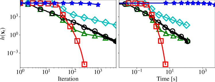
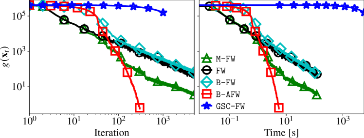
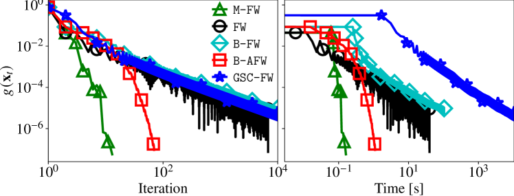
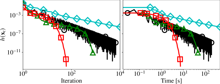
We provide numerical experiments that showcase the performance of the algorithms on generalized self-concordant objectives to complement the theoretical results. In particular, they highlight that the simple step size strategy we propose is competitive with and sometimes outperforms other variants on many instances.

After publication of our initial draft, in a revision of their original work, Dvurechensky et al. [2022] added an analysis of the Away-step Frank-Wolfe algorithm which is complementary to ours (considering a slightly different setup and regimes) and was conducted independently; we have updated the tables to include these additional results.

1.3 Preliminaries and Notation

We denote the domain of f𝑓f as dom(f)=def{𝐱n,f(𝐱)<+}superscriptdefdom𝑓formulae-sequence𝐱superscript𝑛𝑓𝐱\mathrm{dom}(f)\stackrel{{\scriptstyle\mathrm{\scriptscriptstyle def}}}{{=}}\{\mathbf{x}\in\mathbb{R}^{n},f(\mathbf{x})<+\infty\} and the (potentially non-unique) minimizer of Problem (1.1) by 𝐱superscript𝐱\mathbf{x}^{*}. Moreover, we denote the primal gap and the Frank-Wolfe gap at 𝐱𝒳dom(f)𝐱𝒳dom𝑓\mathbf{x}\in\mathcal{X}\cap\mathrm{dom}(f) as h(𝐱)=deff(𝐱)f(𝐱)superscriptdef𝐱𝑓𝐱𝑓superscript𝐱h(\mathbf{x})\stackrel{{\scriptstyle\mathrm{\scriptscriptstyle def}}}{{=}}f(\mathbf{x})-f(\mathbf{x}^{*}) and g(𝐱)=defmax𝐯𝒳f(𝐱),𝐱𝐯superscriptdef𝑔𝐱subscript𝐯𝒳𝑓𝐱𝐱𝐯g(\mathbf{x})\stackrel{{\scriptstyle\mathrm{\scriptscriptstyle def}}}{{=}}\max_{\mathbf{v}\in\mathcal{X}}\left\langle\nabla f(\mathbf{x}),\mathbf{x}-\mathbf{v}\right\rangle, respectively. We use \left\|\cdot\right\|, H\left\|\cdot\right\|_{H}, and ,\left\langle\cdot,\cdot\right\rangle to denote the Euclidean norm, the matrix norm induced by a symmetric positive definite matrix Hn×n𝐻superscript𝑛𝑛H\in\mathbb{R}^{n\times n}, and the Euclidean inner product, respectively. We denote the diameter of 𝒳𝒳\mathcal{X} as D=defmax𝐱,𝐲𝒳𝐱𝐲superscriptdef𝐷subscript𝐱𝐲𝒳norm𝐱𝐲D\stackrel{{\scriptstyle\mathrm{\scriptscriptstyle def}}}{{=}}\max_{\mathbf{x},\mathbf{y}\in\mathcal{X}}\left\|\mathbf{x}-\mathbf{y}\right\|. Given a non-empty set 𝒳n𝒳superscript𝑛\mathcal{X}\subset\mathbb{R}^{n} we refer to its boundary as Bd(𝒳)Bd𝒳\operatorname{Bd}(\mathcal{X}) and to its interior as Int(𝒳)Int𝒳\operatorname{\mathrm{Int}}\left(\mathcal{X}\right). We use ΔnsubscriptΔ𝑛\Delta_{n} to denote the probability simplex of dimension n𝑛n. Given a compact convex set 𝒞dom(f)𝒞dom𝑓\mathcal{C}\subseteq\mathrm{dom}(f) we denote:

Lf𝒞superscriptsubscript𝐿𝑓𝒞\displaystyle L_{f}^{\mathcal{C}} =max𝐮𝒞,𝐝n𝐝2f(𝐮)2𝐝22,absentsubscriptformulae-sequence𝐮𝒞𝐝superscript𝑛superscriptsubscriptnorm𝐝superscript2𝑓𝐮2subscriptsuperscriptnorm𝐝22\displaystyle=\max\limits_{\mathbf{u}\in\mathcal{C},\mathbf{d}\in\mathbb{R}^{n}}\frac{\left\|\mathbf{d}\right\|_{\nabla^{2}f(\mathbf{u})}^{2}}{\left\|\mathbf{d}\right\|^{2}_{2}},
μf𝒞superscriptsubscript𝜇𝑓𝒞\displaystyle\mu_{f}^{\mathcal{C}} =min𝐮𝒞,𝐝n𝐝2f(𝐮)2𝐝22.absentsubscriptformulae-sequence𝐮𝒞𝐝superscript𝑛superscriptsubscriptnorm𝐝superscript2𝑓𝐮2subscriptsuperscriptnorm𝐝22\displaystyle=\min\limits_{\mathbf{u}\in\mathcal{C},\mathbf{d}\in\mathbb{R}^{n}}\frac{\left\|\mathbf{d}\right\|_{\nabla^{2}f(\mathbf{u})}^{2}}{\left\|\mathbf{d}\right\|^{2}_{2}}.

We assume access to:

  1. 1.

    Domain Oracle (DO): Given 𝐱𝒳𝐱𝒳\mathbf{x}\in\mathcal{X}, return true if 𝐱dom(f)𝐱dom𝑓\mathbf{x}\in\mathrm{dom}(f), false otherwise.

  2. 2.

    Zeroth-Order Oracle (ZOO): Given 𝐱dom(f)𝐱dom𝑓\mathbf{x}\in\mathrm{dom}(f), return f(𝐱)𝑓𝐱f(\mathbf{x}).

  3. 3.

    First-Order Oracle (FOO): Given 𝐱dom(f)𝐱dom𝑓\mathbf{x}\in\mathrm{dom}(f), return f(𝐱)𝑓𝐱\nabla f(\mathbf{x}).

  4. 4.

    Linear Minimization Oracle (LMO): Given 𝐝n𝐝superscript𝑛\mathbf{d}\in\mathbb{R}^{n}, return argmin𝐱𝒳𝐱,𝐝subscriptargmin𝐱𝒳𝐱𝐝\operatorname*{argmin}_{\mathbf{x}\in\mathcal{X}}\left\langle\mathbf{x},\mathbf{d}\right\rangle.

The FOO and LMO oracles are standard in the FW literature. The ZOO oracle is often implicitly assumed to be included with the FOO oracle; we make this explicit here for clarity. Finally, the DO oracle is motivated by the properties of generalized self-concordant functions. It is reasonable to assume the availability of the DO oracle: following the definition of the function codomain, one could simply evaluate f𝑓f at 𝐱𝐱\mathbf{x} and assert f(𝐱)<+𝑓𝐱f(\mathbf{x})<+\infty, thereby combining the DO and ZOO oracles into one oracle. However, in many cases testing the membership of 𝐱dom(f)𝐱dom𝑓\mathbf{x}\in\mathrm{dom}(f) is computationally less demanding than the function evaluation.

Remark 1.1.

Requiring access to a zeroth-order and domain oracle are mild assumptions, that were also implicitly assumed in one of the three FW-variants presented in Dvurechensky et al. [2022] when computing the step size according to the strategy from Pedregosa et al. [2020]; see 5 in Algorithm 4. The remaining two variants ensure that 𝐱dom(f)𝐱dom𝑓\mathbf{x}\in\mathrm{dom}(f) by using second-order information about f𝑓f, which we explicitly do not rely on.

The following example motivates the use of Frank-Wolfe algorithms in the context of generalized self-concordant functions. We present more examples in the computational results.

Example 1.2 (Intersection of a convex set with a polytope).

Consider Problem (1.1) where 𝒳=𝒫𝒞𝒳𝒫𝒞\mathcal{X}=\mathcal{P}\cap\mathcal{C}, 𝒫𝒫\mathcal{P} is a polytope over which we can minimize a linear function efficiently, and 𝒞𝒞\mathcal{C} is a convex compact set for which one can easily build a barrier function.
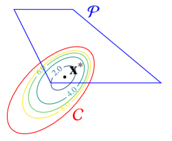
Refer to caption
(a)
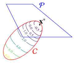
Refer to caption
(b)
Refer to caption
(c)
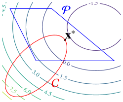
Figure 1: Minimizing f(𝐱)𝑓𝐱f(\mathbf{x}) over 𝒫𝒞𝒫𝒞\mathcal{P}\cap\mathcal{C}, versus minimizing the sum of f(𝐱)𝑓𝐱f(\mathbf{x}) and Φ𝒞(𝐱)subscriptΦ𝒞𝐱\Phi_{\mathcal{C}}(\mathbf{x}) over 𝒫𝒫\mathcal{P} for two different penalty values μsuperscript𝜇\mu^{\prime} and μ𝜇\mu such that μμmuch-greater-thansuperscript𝜇𝜇\mu^{\prime}\gg\mu.

Solving a linear optimization problem over 𝒳𝒳\mathcal{X} may be extremely expensive. In light of this, we can incorporate 𝒞𝒞\mathcal{C} into the problem through the use of a barrier penalty in the objective function, minimizing instead f(𝐱)+μΦ𝒞(𝐱)𝑓𝐱𝜇subscriptΦ𝒞𝐱f(\mathbf{x})+\mu\Phi_{\mathcal{C}}(\mathbf{x}) where Φ𝒞(𝐱)subscriptΦ𝒞𝐱\Phi_{\mathcal{C}}(\mathbf{x}) is a log-barrier function for 𝒞𝒞\mathcal{C} and μ𝜇\mu is a parameter controlling the penalization. This reformulation is illustrated in Figure 1. Note that if the original objective function is generalized self-concordant, so is the new objective function (see Proposition 1 in Sun & Tran-Dinh [2019]). We assume that computing the gradient of f(𝐱)+μΦ𝒞(𝐱)𝑓𝐱𝜇subscriptΦ𝒞𝐱f(\mathbf{x})+\mu\Phi_{\mathcal{C}}(\mathbf{x}) is roughly as expensive as computing the gradient for f(𝐱)𝑓𝐱f(\mathbf{x}) and solving an LP over 𝒫𝒫\mathcal{P} is inexpensive relative to solving an LP over 𝒫𝒞𝒫𝒞\mathcal{P}\cap\mathcal{C}. The μ𝜇\mu parameter can be driven down to 00 after a solution converges in a warm-starting procedure similar to interior-point methods, ensuring convergence to the true optimum.

An additional advantage of this transformation of the problem is the solution structure. Running Frank-Wolfe on the set 𝒫𝒞𝒫𝒞\mathcal{P}\cap\mathcal{C} can select a large number of extremal points from Bd(𝒞)Bd𝒞\operatorname{Bd}(\mathcal{C}) if 𝒞𝒞\mathcal{C} is non-polyhedral. In contrast, 𝒫𝒫\mathcal{P} has a finite number of vertices, a small subset of which will be selected throughout the optimization procedure. The same solution as that of the original problem can thus be constructed as a convex combination of a small number of vertices of 𝒫𝒫\mathcal{P}, improving sparsity and interpretability in many applications.

The following definition formalizes the setting of Problem (1.1).

Definition 1.3 (Generalized self-concordant function).

Let fC3(dom(f))𝑓superscript𝐶3dom𝑓f\in C^{3}\left(\mathrm{dom}(f)\right) be a closed convex function with dom(f)ndom𝑓superscript𝑛\mathrm{dom}(f)\subseteq\mathbb{R}^{n} open. Then f𝑓f is (M,ν)𝑀𝜈\left(M,\nu\right) generalized self-concordant if:

|D3f(𝐱)[𝐰]𝐮,𝐮|M𝐮2f(𝐱)2𝐰2f(𝐱)ν2𝐰23ν,superscriptD3𝑓𝐱delimited-[]𝐰𝐮𝐮𝑀superscriptsubscriptnorm𝐮superscript2𝑓𝐱2superscriptsubscriptnorm𝐰superscript2𝑓𝐱𝜈2superscriptsubscriptnorm𝐰23𝜈\displaystyle|\left\langle\operatorname{D}^{3}f(\mathbf{x})[\mathbf{w}]\mathbf{u},\mathbf{u}\right\rangle|\leq M\left\|\mathbf{u}\right\|_{\nabla^{2}f(\mathbf{x})}^{2}\left\|\mathbf{w}\right\|_{\nabla^{2}f(\mathbf{x})}^{\nu-2}\left\|\mathbf{w}\right\|_{2}^{3-\nu},

for any 𝐱dom(f)𝐱dom𝑓\mathbf{x}\in\mathrm{dom}(f) and 𝐮,𝐰n𝐮𝐰superscript𝑛\mathbf{u},\mathbf{w}\in\mathbb{R}^{n}, where D3f(𝐱)[𝐰]=limα0α1(2f(𝐱+α𝐰)2f(𝐱))superscriptD3𝑓𝐱delimited-[]𝐰subscript𝛼0superscript𝛼1superscript2𝑓𝐱𝛼𝐰superscript2𝑓𝐱\operatorname{D}^{3}f(\mathbf{x})[\mathbf{w}]=\lim\limits_{\alpha\rightarrow 0}\alpha^{-1}\left(\nabla^{2}f(\mathbf{x}+\alpha\mathbf{w})-\nabla^{2}f(\mathbf{x})\right).

2 Frank-Wolfe Convergence Guarantees

We establish convergence rates for a Frank-Wolfe variant with an open-loop step size strategy for generalized self-concordant functions. The Monotonic Frank-Wolfe (M-FW) algorithm presented in Algorithm 1 is a rather simple, but powerful modification of the standard Frank-Wolfe algorithm, with the only difference that before taking a step, we verify if 𝐱t+γt(𝐯t𝐱t)dom(f)subscript𝐱𝑡subscript𝛾𝑡subscript𝐯𝑡subscript𝐱𝑡dom𝑓\mathbf{x}_{t}+\gamma_{t}(\mathbf{v}_{t}-\mathbf{x}_{t})\in\mathrm{dom}(f), and if so, we check whether moving to the next iterate provides primal progress.

Algorithm 1 Monotonic Frank-Wolfe (M-FW)
1:Point 𝐱0𝒳dom(f)subscript𝐱0𝒳dom𝑓\mathbf{x}_{0}\in\mathcal{X}\cap\mathrm{dom}(f), function f𝑓f
2:Iterates 𝐱1,𝒳subscript𝐱1𝒳\mathbf{x}_{1},\dotsc\in\mathcal{X}  
3:for t=0𝑡0t=0 to \dotsc do
4:     𝐯targmin𝐯𝒳f(𝐱t),𝐯subscript𝐯𝑡subscriptargmin𝐯𝒳𝑓subscript𝐱𝑡𝐯\mathbf{v}_{t}\leftarrow\operatorname*{argmin}_{\mathbf{v}\in\mathcal{X}}\left\langle\nabla f(\mathbf{x}_{t}),\mathbf{v}\right\rangle
5:     γt2/(t+2)subscript𝛾𝑡2𝑡2\gamma_{t}\leftarrow 2/(t+2)
6:     𝐱t+1𝐱t+γt(𝐯t𝐱t)subscript𝐱𝑡1subscript𝐱𝑡subscript𝛾𝑡subscript𝐯𝑡subscript𝐱𝑡\mathbf{x}_{t+1}\leftarrow\mathbf{x}_{t}+\gamma_{t}(\mathbf{v}_{t}-\mathbf{x}_{t})
7:     if 𝐱t+1dom(f)subscript𝐱𝑡1dom𝑓\mathbf{x}_{t+1}\notin\mathrm{dom}(f) or f(𝐱t+1)>f(𝐱t)𝑓subscript𝐱𝑡1𝑓subscript𝐱𝑡f(\mathbf{x}_{t+1})>f(\mathbf{x}_{t}) then
8:         𝐱t+1𝐱tsubscript𝐱𝑡1subscript𝐱𝑡\mathbf{x}_{t+1}\leftarrow\mathbf{x}_{t}      

Note, that the open-loop step size rule 2/(t+2)2𝑡22/(t+2) does not guarantee monotonic primal progress for the vanilla Frank-Wolfe algorithm in general. If either of these two checks fails, we simply do not move: the algorithm sets 𝐱t+1=𝐱tsubscript𝐱𝑡1subscript𝐱𝑡\mathbf{x}_{t+1}=\mathbf{x}_{t} in 8 of Algorithm 1. As customary, we assume short-circuit evaluation of the logical conditions in Algorithm 1, i.e., if the first condition in 7 is true, then the second condition is not even checked, and the algorithm directly goes to 8. This minor modification of the vanilla Frank-Wolfe algorithm enables us to use the monotonicity of the iterates in the proofs to come, at the expense of at most one extra function evaluation per iteration. Note that if we set 𝐱t+1=𝐱tsubscript𝐱𝑡1subscript𝐱𝑡\mathbf{x}_{t+1}=\mathbf{x}_{t}, we do not need to call the FOO or LMO oracle at iteration t+1𝑡1t+1, as we can simply reuse f(𝐱t)𝑓subscript𝐱𝑡\nabla f(\mathbf{x}_{t}) and 𝐯tsubscript𝐯𝑡\mathbf{v}_{t}. This effectively means that between successive iterations in which we search for an acceptable value of γtsubscript𝛾𝑡\gamma_{t}, we only need to call the zeroth-order and domain oracle.

In order to establish the main convergence results for the algorithm, we lower bound the progress per iteration with the help of Proposition 2.1.

Proposition 2.1.

(C.f., Sun & Tran-Dinh [2019, Proposition 10]) Given a (M,ν)𝑀𝜈\left(M,\nu\right) generalized self-concordant function, then for ν2𝜈2\nu\geq 2, we have that:

f(𝐲)f(𝐱)f(𝐱),𝐲𝐱ων(dν(𝐱𝐲))𝐲𝐱2f(𝐱)2,𝑓𝐲𝑓𝐱𝑓𝐱𝐲𝐱subscript𝜔𝜈subscript𝑑𝜈𝐱𝐲superscriptsubscriptnorm𝐲𝐱superscript2𝑓𝐱2\displaystyle f(\mathbf{y})-f(\mathbf{x})-\left\langle\nabla f(\mathbf{x}),\mathbf{y}-\mathbf{x}\right\rangle\leq\omega_{\nu}(d_{\nu}(\mathbf{x}-\mathbf{y}))\left\|\mathbf{y}-\mathbf{x}\right\|_{\nabla^{2}f(\mathbf{x})}^{2}, (2.1)

where the inequality holds if and only if dν(𝐱,𝐲)<1subscript𝑑𝜈𝐱𝐲1d_{\nu}(\mathbf{x},\mathbf{y})<1 for ν>2𝜈2\nu>2, and we have that,

dν(𝐱,𝐲)=def{M𝐲𝐱if ν=2(ν21)M𝐲𝐱3ν𝐲𝐱2f(𝐱)ν2if ν>2,superscriptdefsubscript𝑑𝜈𝐱𝐲cases𝑀norm𝐲𝐱if 𝜈2𝜈21𝑀superscriptnorm𝐲𝐱3𝜈superscriptsubscriptnorm𝐲𝐱superscript2𝑓𝐱𝜈2if 𝜈2d_{\nu}(\mathbf{x},\mathbf{y})\stackrel{{\scriptstyle\mathrm{\scriptscriptstyle def}}}{{=}}\begin{cases}M\left\|\mathbf{y}-\mathbf{x}\right\|&\mbox{if }\nu=2\\ (\frac{\nu}{2}-1)M\left\|\mathbf{y}-\mathbf{x}\right\|^{3-\nu}\left\|\mathbf{y}-\mathbf{x}\right\|_{\nabla^{2}f(\mathbf{x})}^{\nu-2}&\mbox{if }\nu>2,\end{cases} (2.2)

where:

ων(τ)=def{eττ1τ2if ν=2τln(1τ)τ2if ν=3(1τ)ln(1τ)+ττ2if ν=4(ν24ν)1τ[ν22(3ν)τ((1τ)2(3ν)2ν1)1]otherwise.superscriptdefsubscript𝜔𝜈𝜏casessuperscript𝑒𝜏𝜏1superscript𝜏2if 𝜈2𝜏ln1𝜏superscript𝜏2if 𝜈31𝜏ln1𝜏𝜏superscript𝜏2if 𝜈4𝜈24𝜈1𝜏delimited-[]𝜈223𝜈𝜏superscript1𝜏23𝜈2𝜈11otherwise.\omega_{\nu}(\tau)\stackrel{{\scriptstyle\mathrm{\scriptscriptstyle def}}}{{=}}\begin{cases}\frac{e^{\tau}-\tau-1}{\tau^{2}}&\mbox{if }\nu=2\\ \frac{-\tau-\text{ln}(1-\tau)}{\tau^{2}}&\mbox{if }\nu=3\\ \frac{(1-\tau)\text{ln}(1-\tau)+\tau}{\tau^{2}}&\mbox{if }\nu=4\\ \left(\frac{\nu-2}{4-\nu}\right)\,\,\frac{1}{\tau}\left[\frac{\nu-2}{2(3-\nu)\tau}\left((1-\tau)^{\frac{2(3-\nu)}{2-\nu}}-1\right)-1\right]&\mbox{otherwise.}\end{cases}

The inequality shown in Equation (2.1) is very similar to the one that we would obtain if the gradient of f𝑓f were Lipschitz continuous, however, while the Lipschitz continuity of the gradient leads to an inequality that holds globally for all 𝐱,𝐲dom(f)𝐱𝐲dom𝑓\mathbf{x},\mathbf{y}\in\mathrm{dom}(f), the inequality in Equation (2.1) only holds for dν(𝐱,𝐲)<1subscript𝑑𝜈𝐱𝐲1d_{\nu}(\mathbf{x},\mathbf{y})<1. Moreover, there are two other important differences, the norm used in Equation (2.1) is now the norm defined by the Hessian at 𝐱tsubscript𝐱𝑡\mathbf{x}_{t} instead of the 2subscript2\ell_{2} norm, and the term multiplying the norm is ων(dν(𝐱,𝐲))subscript𝜔𝜈subscript𝑑𝜈𝐱𝐲\omega_{\nu}(d_{\nu}(\mathbf{x},\mathbf{y})) instead of 1/2121/2. We deal with the latter issue by bounding ων(dν(𝐱,𝐲))subscript𝜔𝜈subscript𝑑𝜈𝐱𝐲\omega_{\nu}(d_{\nu}(\mathbf{x},\mathbf{y})) with a constant that depends on ν𝜈\nu for any 𝐱,𝐲dom(f)𝐱𝐲dom𝑓\mathbf{x},\mathbf{y}\in\mathrm{dom}(f) such that dν(𝐱,𝐲)1/2subscript𝑑𝜈𝐱𝐲12d_{\nu}(\mathbf{x},\mathbf{y})\leq 1/2, as shown in Remark 2.2.

Remark 2.2.

As dων(τ)/dτ>0dsubscript𝜔𝜈𝜏d𝜏0\operatorname{d}{\omega_{\nu}(\tau)}/\operatorname{d}{\tau}>0 for τ<1𝜏1\tau<1 and ν2𝜈2\nu\geq 2, then ων(τ)ων(1/2)subscript𝜔𝜈𝜏subscript𝜔𝜈12\omega_{\nu}(\tau)\leq\omega_{\nu}(1/2) for τ1/2𝜏12\tau\leq 1/2.

Due to the fact that we use a simple step size γt=2/(t+2)subscript𝛾𝑡2𝑡2\gamma_{t}=2/(t+2), that we make monotonic progress, and we ensure that the iterates are inside dom(f)dom𝑓\mathrm{dom}(f), careful accounting allows us to bound the number of iterations until dν(𝐱t,𝐱t+γt(𝐯t𝐱t))1/2subscript𝑑𝜈subscript𝐱𝑡subscript𝐱𝑡subscript𝛾𝑡subscript𝐯𝑡subscript𝐱𝑡12d_{\nu}(\mathbf{x}_{t},\mathbf{x}_{t}+\gamma_{t}(\mathbf{v}_{t}-\mathbf{x}_{t}))\leq 1/2. Before formalizing the convergence rate we first review a lemma that we will need in the proof.

Lemma 2.3.

(C.f., [Sun & Tran-Dinh, 2019, Proposition 7]) Let f𝑓f be a generalized self-concordant function with ν>2𝜈2\nu>2. If dν(𝐱,𝐲)<1subscript𝑑𝜈𝐱𝐲1d_{\nu}(\mathbf{x},\mathbf{y})<1 and 𝐱dom(f)𝐱dom𝑓\mathbf{x}\in\mathrm{dom}(f) then 𝐲dom(f)𝐲dom𝑓\mathbf{y}\in\mathrm{dom}(f). For the case ν=2𝜈2\nu=2 we have that dom(f)=ndom𝑓superscript𝑛\mathrm{dom}(f)=\mathbb{R}^{n}.

Putting all these things together allows us to obtain a convergence rate for Algorithm 1.

Theorem 2.4.

Suppose 𝒳𝒳\mathcal{X} is a compact convex set and f𝑓f is a (M,ν)𝑀𝜈\left(M,\nu\right) generalized self-concordant function with ν2𝜈2\nu\geq 2. Then, the Monotonic Frank-Wolfe algorithm (Algorithm 1) satisfies:

h(𝐱t)4(Tν+1)t+1max{h(𝐱0),Lf0D2ων(1/2)}.subscript𝐱𝑡4subscript𝑇𝜈1𝑡1subscript𝐱0superscriptsubscript𝐿𝑓subscript0superscript𝐷2subscript𝜔𝜈12\displaystyle h(\mathbf{x}_{t})\leq\frac{4(T_{\nu}+1)}{t+1}\max\left\{h(\mathbf{x}_{0}),L_{f}^{\mathcal{L}_{0}}D^{2}\omega_{\nu}(1/2)\right\}. (2.3)

for tTν𝑡subscript𝑇𝜈t\geq T_{\nu}, where Lf0=max𝐮0,𝐝n𝐝2f(𝐮)2/𝐝22superscriptsubscript𝐿𝑓subscript0subscriptformulae-sequence𝐮subscript0𝐝superscript𝑛superscriptsubscriptnorm𝐝superscript2𝑓𝐮2subscriptsuperscriptnorm𝐝22L_{f}^{\mathcal{L}_{0}}=\max\limits_{\mathbf{u}\in\mathcal{L}_{0},\mathbf{d}\in\mathbb{R}^{n}}\left\|\mathbf{d}\right\|_{\nabla^{2}f(\mathbf{u})}^{2}/\left\|\mathbf{d}\right\|^{2}_{2} and Tνsubscript𝑇𝜈T_{\nu} is defined as:

Tν=def{4MD2if ν=22MD(Lf0)ν/21(ν2)2otherwise.superscriptdefsubscript𝑇𝜈cases4𝑀𝐷2if 𝜈22𝑀𝐷superscriptsuperscriptsubscript𝐿𝑓subscript0𝜈21𝜈22otherwiseT_{\nu}\stackrel{{\scriptstyle\mathrm{\scriptscriptstyle def}}}{{=}}\begin{cases}\left\lceil 4MD\right\rceil-2&\mbox{if }\nu=2\\ \left\lceil 2MD(L_{f}^{\mathcal{L}_{0}})^{\nu/2-1}(\nu-2)\right\rceil-2&\mbox{otherwise}.\end{cases} (2.4)

Otherwise it holds that h(𝐱t)h(𝐱0)subscript𝐱𝑡subscript𝐱0h(\mathbf{x}_{t})\leq h(\mathbf{x}_{0}) for t<Tν𝑡subscript𝑇𝜈t<T_{\nu}.

  • Proof.

    Consider the compact set 0=def{𝐱dom(f)𝒳f(𝐱)f(𝐱0)}superscriptdefsubscript0conditional-set𝐱dom𝑓𝒳𝑓𝐱𝑓subscript𝐱0\mathcal{L}_{0}\stackrel{{\scriptstyle\mathrm{\scriptscriptstyle def}}}{{=}}\left\{\mathbf{x}\in\mathrm{dom}(f)\cap\mathcal{X}\mid f(\mathbf{x})\leq f(\mathbf{x}_{0})\right\}. As the algorithm makes monotonic progress and moves towards points such that 𝐱t𝒳subscript𝐱𝑡𝒳\mathbf{x}_{t}\in\mathcal{X}, then 𝐱t0subscript𝐱𝑡subscript0\mathbf{x}_{t}\in\mathcal{L}_{0} for t0𝑡0t\geq 0. As the smoothness parameter of f𝑓f is bounded over 0subscript0\mathcal{L}_{0}, we have from the properties of smooth functions that the bound 𝐝2f(𝐱t)2/𝐝2Lf0subscriptsuperscriptnorm𝐝2superscript2𝑓subscript𝐱𝑡superscriptnorm𝐝2superscriptsubscript𝐿𝑓subscript0\left\|\mathbf{d}\right\|^{2}_{\nabla^{2}f(\mathbf{x}_{t})}/\left\|\mathbf{d}\right\|^{2}\leq L_{f}^{\mathcal{L}_{0}} holds for any 𝐝n𝐝superscript𝑛\mathbf{d}\in\mathbb{R}^{n}. Particularizing for 𝐝=𝐱t𝐯t𝐝subscript𝐱𝑡subscript𝐯𝑡\mathbf{d}=\mathbf{x}_{t}-\mathbf{v}_{t} and noting that 𝐱t𝐯tDnormsubscript𝐱𝑡subscript𝐯𝑡𝐷\left\|\mathbf{x}_{t}-\mathbf{v}_{t}\right\|\leq D leads to 𝐱t𝐯t2f(𝐱t)2Lf0D2subscriptsuperscriptnormsubscript𝐱𝑡subscript𝐯𝑡2superscript2𝑓subscript𝐱𝑡superscriptsubscript𝐿𝑓subscript0superscript𝐷2\left\|\mathbf{x}_{t}-\mathbf{v}_{t}\right\|^{2}_{\nabla^{2}f(\mathbf{x}_{t})}\leq L_{f}^{\mathcal{L}_{0}}D^{2}. We then define Tνsubscript𝑇𝜈T_{\nu} as:

    Tν=def{4MD2if ν=22MD(Lf0)ν/21(ν2)2otherwise.superscriptdefsubscript𝑇𝜈cases4𝑀𝐷2if 𝜈22𝑀𝐷superscriptsuperscriptsubscript𝐿𝑓subscript0𝜈21𝜈22otherwiseT_{\nu}\stackrel{{\scriptstyle\mathrm{\scriptscriptstyle def}}}{{=}}\begin{cases}\left\lceil 4MD\right\rceil-2&\mbox{if }\nu=2\\ \left\lceil 2MD(L_{f}^{\mathcal{L}_{0}})^{\nu/2-1}(\nu-2)\right\rceil-2&\mbox{otherwise}.\end{cases}

    Using the definition shown in Equation (2.2) we have that for tTν𝑡subscript𝑇𝜈t\geq T_{\nu} then d(𝐱t,𝐱t+γt(𝐯t𝐱t))1/2𝑑subscript𝐱𝑡subscript𝐱𝑡subscript𝛾𝑡subscript𝐯𝑡subscript𝐱𝑡12d(\mathbf{x}_{t},\mathbf{x}_{t}+\gamma_{t}(\mathbf{v}_{t}-\mathbf{x}_{t}))\leq 1/2. This fact, along with the fact that 𝐱tdom(f)subscript𝐱𝑡dom𝑓\mathbf{x}_{t}\in\mathrm{dom}(f) (by monotonicity) allows us to claim that 𝐱t+γt(𝐯t𝐱t)dom(f)subscript𝐱𝑡subscript𝛾𝑡subscript𝐯𝑡subscript𝐱𝑡dom𝑓\mathbf{x}_{t}+\gamma_{t}(\mathbf{v}_{t}-\mathbf{x}_{t})\in\mathrm{dom}(f), by application of Lemma 2.3. This means that the non-zero step size γtsubscript𝛾𝑡\gamma_{t} will ensure that 𝐱t+γt(𝐯t𝐱t)dom(f)subscript𝐱𝑡subscript𝛾𝑡subscript𝐯𝑡subscript𝐱𝑡dom𝑓\mathbf{x}_{t}+\gamma_{t}(\mathbf{v}_{t}-\mathbf{x}_{t})\in\mathrm{dom}(f) in 7 of Algorithm 1. Moreover, it allows us to use the bound between the function value at points 𝐱tsubscript𝐱𝑡\mathbf{x}_{t} and 𝐱t+γt(𝐯t𝐱t)subscript𝐱𝑡subscript𝛾𝑡subscript𝐯𝑡subscript𝐱𝑡\mathbf{x}_{t}+\gamma_{t}\left(\mathbf{v}_{t}-\mathbf{x}_{t}\right) in Equation (2.1) of Proposition 2.1, which holds for d(𝐱t,𝐱t+γt(𝐯t𝐱t))<1𝑑subscript𝐱𝑡subscript𝐱𝑡subscript𝛾𝑡subscript𝐯𝑡subscript𝐱𝑡1d(\mathbf{x}_{t},\mathbf{x}_{t}+\gamma_{t}\left(\mathbf{v}_{t}-\mathbf{x}_{t}\right))<1. With this we can estimate the primal progress we can guarantee for tTν𝑡subscript𝑇𝜈t\geq T_{\nu} if we move from 𝐱tsubscript𝐱𝑡\mathbf{x}_{t} to 𝐱t+γt(𝐯t𝐱t)subscript𝐱𝑡subscript𝛾𝑡subscript𝐯𝑡subscript𝐱𝑡\mathbf{x}_{t}+\gamma_{t}\left(\mathbf{v}_{t}-\mathbf{x}_{t}\right):

    h(𝐱t+γt(𝐯t𝐱t))subscript𝐱𝑡subscript𝛾𝑡subscript𝐯𝑡subscript𝐱𝑡\displaystyle h(\mathbf{x}_{t}+\gamma_{t}\left(\mathbf{v}_{t}-\mathbf{x}_{t}\right)) h(𝐱t)γtg(𝐱t)+γt2ων(dν(𝐱t,𝐱t+γt(𝐯t𝐱t)))𝐯t𝐱t2f(𝐱t)2absentsubscript𝐱𝑡subscript𝛾𝑡𝑔subscript𝐱𝑡superscriptsubscript𝛾𝑡2subscript𝜔𝜈subscript𝑑𝜈subscript𝐱𝑡subscript𝐱𝑡subscript𝛾𝑡subscript𝐯𝑡subscript𝐱𝑡subscriptsuperscriptnormsubscript𝐯𝑡subscript𝐱𝑡2superscript2𝑓subscript𝐱𝑡\displaystyle\leq h(\mathbf{x}_{t})-\gamma_{t}g(\mathbf{x}_{t})+\gamma_{t}^{2}\omega_{\nu}\left(d_{\nu}\left(\mathbf{x}_{t},\mathbf{x}_{t}+\gamma_{t}\left(\mathbf{v}_{t}-\mathbf{x}_{t}\right)\right)\right)\left\|\mathbf{v}_{t}-\mathbf{x}_{t}\right\|^{2}_{\nabla^{2}f(\mathbf{x}_{t})}
    h(𝐱t)(1γt)+γt2Lf0D2ων(1/2),absentsubscript𝐱𝑡1subscript𝛾𝑡superscriptsubscript𝛾𝑡2superscriptsubscript𝐿𝑓subscript0superscript𝐷2subscript𝜔𝜈12\displaystyle\leq h(\mathbf{x}_{t})\left(1-\gamma_{t}\right)+\gamma_{t}^{2}L_{f}^{\mathcal{L}_{0}}D^{2}\omega_{\nu}(1/2),

    where the second inequality follows from the upper bound on the primal gap via the Frank-Wolfe gap g(𝐱t)𝑔subscript𝐱𝑡g(\mathbf{x}_{t}), the application of Remark 2.2 as for tTν𝑡subscript𝑇𝜈t\geq T_{\nu} we have that dν(𝐱t,𝐱t+γt(𝐯t𝐱t))1/2subscript𝑑𝜈subscript𝐱𝑡subscript𝐱𝑡subscript𝛾𝑡subscript𝐯𝑡subscript𝐱𝑡12d_{\nu}(\mathbf{x}_{t},\mathbf{x}_{t}+\gamma_{t}\left(\mathbf{v}_{t}-\mathbf{x}_{t}\right))\leq 1/2, and from the fact that 𝐱t0subscript𝐱𝑡subscript0\mathbf{x}_{t}\in\mathcal{L}_{0} for all t0𝑡0t\geq 0. With the previous chain of inequalities we can bound the primal progress for tTν𝑡subscript𝑇𝜈t\geq T_{\nu} as

    h(𝐱t)h(𝐱t+γt(𝐯t𝐱t))subscript𝐱𝑡subscript𝐱𝑡subscript𝛾𝑡subscript𝐯𝑡subscript𝐱𝑡\displaystyle h(\mathbf{x}_{t})-h(\mathbf{x}_{t}+\gamma_{t}\left(\mathbf{v}_{t}-\mathbf{x}_{t}\right)) γth(𝐱t)γt2Lf0D2ων(1/2).absentsubscript𝛾𝑡subscript𝐱𝑡superscriptsubscript𝛾𝑡2superscriptsubscript𝐿𝑓subscript0superscript𝐷2subscript𝜔𝜈12\displaystyle\geq\gamma_{t}h(\mathbf{x}_{t})-\gamma_{t}^{2}L_{f}^{\mathcal{L}_{0}}D^{2}\omega_{\nu}(1/2). (2.5)

    From these facts we can prove the convergence rate shown in Equation (2.3) by induction. The base case t=Tν𝑡subscript𝑇𝜈t=T_{\nu} holds trivially by the fact that using monotonicity we have that h(𝐱Tν)h(𝐱0)subscript𝐱subscript𝑇𝜈subscript𝐱0h(\mathbf{x}_{T_{\nu}})\leq h(\mathbf{x}_{0}). Assuming the claim is true for some tTν𝑡subscript𝑇𝜈t\geq T_{\nu} we distinguish two cases.
    Case γth(𝐱t)γt2Lf0D2ων(1/2)>0subscript𝛾𝑡subscript𝐱𝑡superscriptsubscript𝛾𝑡2superscriptsubscript𝐿𝑓subscript0superscript𝐷2subscript𝜔𝜈120\gamma_{t}h(\mathbf{x}_{t})-\gamma_{t}^{2}L_{f}^{\mathcal{L}_{0}}D^{2}\omega_{\nu}(1/2)>0: Focusing on the first case, we can plug the previous inequality into Equation (2.5) to find that γtsubscript𝛾𝑡\gamma_{t} guarantees primal progress, that is, h(𝐱t)>h(𝐱t+γt(𝐯t𝐱t))subscript𝐱𝑡subscript𝐱𝑡subscript𝛾𝑡subscript𝐯𝑡subscript𝐱𝑡h(\mathbf{x}_{t})>h(\mathbf{x}_{t}+\gamma_{t}\left(\mathbf{v}_{t}-\mathbf{x}_{t}\right)) with the step size γtsubscript𝛾𝑡\gamma_{t}, and so we know that we will not go into 8 of Algorithm 1, and we have that h(𝐱t+1)=h(𝐱t+γt(𝐯t𝐱t))subscript𝐱𝑡1subscript𝐱𝑡subscript𝛾𝑡subscript𝐯𝑡subscript𝐱𝑡h(\mathbf{x}_{t+1})=h(\mathbf{x}_{t}+\gamma_{t}\left(\mathbf{v}_{t}-\mathbf{x}_{t}\right)). Thus using the induction hypothesis and plugging in the expression for γt=2/(t+2)subscript𝛾𝑡2𝑡2\gamma_{t}=2/(t+2) into Equation (2.5) we have:

    h(𝐱t+1)subscript𝐱𝑡1\displaystyle h(\mathbf{x}_{t+1}) 4max{h(𝐱0),Lf0D2ων(1/2)}((Tν+1)t(t+1)(t+2)+1(t+2)2)absent4subscript𝐱0superscriptsubscript𝐿𝑓subscript0superscript𝐷2subscript𝜔𝜈12subscript𝑇𝜈1𝑡𝑡1𝑡21superscript𝑡22\displaystyle\leq 4\max\left\{h(\mathbf{x}_{0}),L_{f}^{\mathcal{L}_{0}}D^{2}\omega_{\nu}(1/2)\right\}\left(\frac{(T_{\nu}+1)t}{(t+1)(t+2)}+\frac{1}{(t+2)^{2}}\right)
    4(Tν+1)t+2max{h(𝐱0),Lf0D2ων(1/2)},absent4subscript𝑇𝜈1𝑡2subscript𝐱0superscriptsubscript𝐿𝑓subscript0superscript𝐷2subscript𝜔𝜈12\displaystyle\leq\frac{4(T_{\nu}+1)}{t+2}\max\left\{h(\mathbf{x}_{0}),L_{f}^{\mathcal{L}_{0}}D^{2}\omega_{\nu}(1/2)\right\},

    where we use that (Tν+1)t/(t+1)+1/(t+2)Tν+1subscript𝑇𝜈1𝑡𝑡11𝑡2subscript𝑇𝜈1(T_{\nu}+1)t/(t+1)+1/(t+2)\leq T_{\nu}+1 for all t0𝑡0t\geq 0 and any tTν𝑡subscript𝑇𝜈t\geq T_{\nu}.
    Case γth(𝐱t)γt2Lf0D2ων(1/2)0subscript𝛾𝑡subscript𝐱𝑡superscriptsubscript𝛾𝑡2superscriptsubscript𝐿𝑓subscript0superscript𝐷2subscript𝜔𝜈120\gamma_{t}h(\mathbf{x}_{t})-\gamma_{t}^{2}L_{f}^{\mathcal{L}_{0}}D^{2}\omega_{\nu}(1/2)\leq 0: In this case, we cannot guarantee that the step size γtsubscript𝛾𝑡\gamma_{t} provides primal progress by plugging into Equation (2.5), and so we cannot guarantee if a step size of γtsubscript𝛾𝑡\gamma_{t} will be accepted and we will have 𝐱t+1=𝐱t+γt(𝐯t𝐱t)subscript𝐱𝑡1subscript𝐱𝑡subscript𝛾𝑡subscript𝐯𝑡subscript𝐱𝑡\mathbf{x}_{t+1}=\mathbf{x}_{t}+\gamma_{t}\left(\mathbf{v}_{t}-\mathbf{x}_{t}\right), or we will simply have 𝐱t+1=𝐱tsubscript𝐱𝑡1subscript𝐱𝑡\mathbf{x}_{t+1}=\mathbf{x}_{t}, that is, we may go into 8 of Algorithm 1. Nevertheless, if we reorganize the expression γth(𝐱t)γt2Lf0D2ων(1/2)0subscript𝛾𝑡subscript𝐱𝑡superscriptsubscript𝛾𝑡2superscriptsubscript𝐿𝑓subscript0superscript𝐷2subscript𝜔𝜈120\gamma_{t}h(\mathbf{x}_{t})-\gamma_{t}^{2}L_{f}^{\mathcal{L}_{0}}D^{2}\omega_{\nu}(1/2)\leq 0, by monotonicity we will have that:

    h(𝐱t+1)h(𝐱t)2t+2Lf0D2ων(1/2)4(Tν+1)t+2max{h(𝐱0),Lf0D2ων(1/2)}.subscript𝐱𝑡1subscript𝐱𝑡2𝑡2superscriptsubscript𝐿𝑓subscript0superscript𝐷2subscript𝜔𝜈124subscript𝑇𝜈1𝑡2subscript𝐱0superscriptsubscript𝐿𝑓subscript0superscript𝐷2subscript𝜔𝜈12\displaystyle h(\mathbf{x}_{t+1})\leq h(\mathbf{x}_{t})\leq\frac{2}{t+2}L_{f}^{\mathcal{L}_{0}}D^{2}\omega_{\nu}(1/2)\leq\frac{4(T_{\nu}+1)}{t+2}\max\left\{h(\mathbf{x}_{0}),L_{f}^{\mathcal{L}_{0}}D^{2}\omega_{\nu}(1/2)\right\}.

    Where the last inequality holds as 24(Tν+1)24subscript𝑇𝜈12\leq 4(T_{\nu}+1) for any Tν0subscript𝑇𝜈0T_{\nu}\geq 0. ∎

One of the quantities that we have used in the proof of Theorem 2.4 is Lf0superscriptsubscript𝐿𝑓subscript0L_{f}^{\mathcal{L}_{0}}. Note that the function f𝑓f is Lf0superscriptsubscript𝐿𝑓subscript0L_{f}^{\mathcal{L}_{0}}-smooth over 0subscript0\mathcal{L}_{0}. One could wonder why we have bothered to use the bound on the Bregman divergence in Proposition 2.1 for a (M,ν)𝑀𝜈(M,\nu)-generalized self-concordant function, instead of simply using the bounds from the Lf0superscriptsubscript𝐿𝑓subscript0L_{f}^{\mathcal{L}_{0}}-smoothness of f𝑓f over 0subscript0\mathcal{L}_{0}. The reason is that the upper bound on the Bregman divergence in Proposition 2.1 applies for any 𝐱,𝐲dom(f)𝐱𝐲dom𝑓\mathbf{x},\mathbf{y}\in\mathrm{dom}(f) such that dν(𝐱,𝐲)<1subscript𝑑𝜈𝐱𝐲1d_{\nu}(\mathbf{x},\mathbf{y})<1, and we can easily bound the number of iterations Tνsubscript𝑇𝜈T_{\nu} it takes for the step size γt=2/(t+2)subscript𝛾𝑡2𝑡2\gamma_{t}=2/(t+2) to verify both 𝐱t,𝐱t+γt(𝐯t𝐱t)dom(f)subscript𝐱𝑡subscript𝐱𝑡subscript𝛾𝑡subscript𝐯𝑡subscript𝐱𝑡dom𝑓\mathbf{x}_{t},\mathbf{x}_{t}+\gamma_{t}(\mathbf{v}_{t}-\mathbf{x}_{t})\in\mathrm{dom}(f) and dν(𝐱t,𝐱t+γt(𝐯t𝐱t))<1subscript𝑑𝜈subscript𝐱𝑡subscript𝐱𝑡subscript𝛾𝑡subscript𝐯𝑡subscript𝐱𝑡1d_{\nu}(\mathbf{x}_{t},\mathbf{x}_{t}+\gamma_{t}(\mathbf{v}_{t}-\mathbf{x}_{t}))<1 for tTν𝑡subscript𝑇𝜈t\geq T_{\nu}. However, in order to apply the bound on the Bregman divergence from Lf0superscriptsubscript𝐿𝑓subscript0L_{f}^{\mathcal{L}_{0}}-smoothness we need 𝐱t,𝐱t+γt(𝐯t𝐱t)0subscript𝐱𝑡subscript𝐱𝑡subscript𝛾𝑡subscript𝐯𝑡subscript𝐱𝑡subscript0\mathbf{x}_{t},\mathbf{x}_{t}+\gamma_{t}(\mathbf{v}_{t}-\mathbf{x}_{t})\in\mathcal{L}_{0}, and while it is easy to show by monotonicity that 𝐱t0subscript𝐱𝑡subscript0\mathbf{x}_{t}\in\mathcal{L}_{0}, there is no straightforward way to prove that for some T~νsubscript~𝑇𝜈\tilde{T}_{\nu} we have that 𝐱t+γt(𝐯t𝐱t)0subscript𝐱𝑡subscript𝛾𝑡subscript𝐯𝑡subscript𝐱𝑡subscript0\mathbf{x}_{t}+\gamma_{t}(\mathbf{v}_{t}-\mathbf{x}_{t})\in\mathcal{L}_{0} for all tT~ν𝑡subscript~𝑇𝜈t\geq\tilde{T}_{\nu}, i.e., that from some point onward a step with a non-zero step size is taken (that is, we do not go into 8 of Algorithm 1) that guarantees primal progress.

Remark 2.5.

In the case where ν=2𝜈2\nu=2 we can easily bound the primal gap h(𝐱1)subscript𝐱1h(\mathbf{x}_{1}), as in this setting dom(f)=ndom𝑓superscript𝑛\mathrm{dom}(f)=\mathbb{R}^{n}, which leads to h(𝐱1)Lf𝒳D2subscript𝐱1superscriptsubscript𝐿𝑓𝒳superscript𝐷2h(\mathbf{x}_{1})\leq L_{f}^{\mathcal{X}}D^{2} from Equation (2.5), regardless of if we set 𝐱1=𝐱0subscript𝐱1subscript𝐱0\mathbf{x}_{1}=\mathbf{x}_{0} or 𝐱1=𝐯0subscript𝐱1subscript𝐯0\mathbf{x}_{1}=\mathbf{v}_{0}. Moreover, as the upper bound on the Bregman divergence holds for ν=2𝜈2\nu=2 regardless of the value of d2(𝐱,𝐲)subscript𝑑2𝐱𝐲d_{2}(\mathbf{x},\mathbf{y}), we can modify the proof of Theorem 2.4 to obtain a convergence rate of the form h(𝐱t)2/(t+1)Lf𝒳D2w2(MD)subscript𝐱𝑡2𝑡1superscriptsubscript𝐿𝑓𝒳superscript𝐷2subscript𝑤2𝑀𝐷h(\mathbf{x}_{t})\leq 2/(t+1)L_{f}^{\mathcal{X}}D^{2}w_{2}(MD) for t1𝑡1t\geq 1, which is reminiscient of the 𝒪(Lf𝒳D2/t)𝒪superscriptsubscript𝐿𝑓𝒳superscript𝐷2𝑡\mathcal{O}(L_{f}^{\mathcal{X}}D^{2}/t) rate of the original Frank-Wolfe algorithm for the smooth and convex case.

Furthermore, with this simple step size we can also prove a convergence rate for the Frank-Wolfe gap, as shown in Theorem 2.6. More specifically, the minimum of the Frank-Wolfe gap over the run of the algorithm converges at a rate of 𝒪(1/t)𝒪1𝑡\mathcal{O}(1/t). The idea of the proof is very similar to the one in Jaggi [2013]. In a nutshell, as the primal progress per iteration is directly related to the step size times the Frank-Wolfe gap, we know that the Frank-Wolfe gap cannot remain indefinitely above a given value, as otherwise we would obtain a large amount of primal progress, which would make the primal gap become negative. This is formalized in Theorem 2.6.

Theorem 2.6.

Suppose 𝒳𝒳\mathcal{X} is a compact convex set and f𝑓f is a (M,ν)𝑀𝜈\left(M,\nu\right) generalized self-concordant function with ν2𝜈2\nu\geq 2. Then if the Monotonic Frank-Wolfe algorithm (Algorithm 1) is run for TTν+6𝑇subscript𝑇𝜈6T\geq T_{\nu}+6 iterations, we will have that:

min1tTg(𝐱t)𝒪(1/T),subscript1𝑡𝑇𝑔subscript𝐱𝑡𝒪1𝑇\displaystyle\min\limits_{1\leq t\leq T}g(\mathbf{x}_{t})\leq\mathcal{O}(1/T),

where Tνsubscript𝑇𝜈T_{\nu} is defined as:

Tν=def{4MD2if ν=22MD(Lf0)ν/21(ν2)2otherwise.superscriptdefsubscript𝑇𝜈cases4𝑀𝐷2if 𝜈22𝑀𝐷superscriptsuperscriptsubscript𝐿𝑓subscript0𝜈21𝜈22otherwiseT_{\nu}\stackrel{{\scriptstyle\mathrm{\scriptscriptstyle def}}}{{=}}\begin{cases}\left\lceil 4MD\right\rceil-2&\mbox{if }\nu=2\\ \left\lceil 2MD(L_{f}^{\mathcal{L}_{0}})^{\nu/2-1}(\nu-2)\right\rceil-2&\mbox{otherwise}.\end{cases} (2.6)
  • Proof.

    In order to prove the claim, we focus on the iterations Tν+(TTν)/32tT2subscript𝑇𝜈𝑇subscript𝑇𝜈32𝑡𝑇2T_{\nu}+\lceil(T-T_{\nu})/3\rceil-2\leq t\leq T-2, where Tνsubscript𝑇𝜈T_{\nu} is defined in Equation (2.6). Note that as we assume that TTν+6𝑇subscript𝑇𝜈6T\geq T_{\nu}+6, we know that TνTν+(TTν)/32subscript𝑇𝜈subscript𝑇𝜈𝑇subscript𝑇𝜈32T_{\nu}\leq T_{\nu}+\lceil(T-T_{\nu})/3\rceil-2, and so for iterations Tν+(TTν)/32tT2subscript𝑇𝜈𝑇subscript𝑇𝜈32𝑡𝑇2T_{\nu}+\lceil(T-T_{\nu})/3\rceil-2\leq t\leq T-2 we know that dν(𝐱t,𝐱t+1)1/2subscript𝑑𝜈subscript𝐱𝑡subscript𝐱𝑡112d_{\nu}(\mathbf{x}_{t},\mathbf{x}_{t+1})\leq 1/2, and so:

    h(𝐱t+1)subscript𝐱𝑡1\displaystyle h(\mathbf{x}_{t+1}) h(𝐱t)γtg(𝐱t)+γt2Lf0D2ων(1/2).absentsubscript𝐱𝑡subscript𝛾𝑡𝑔subscript𝐱𝑡superscriptsubscript𝛾𝑡2superscriptsubscript𝐿𝑓subscript0superscript𝐷2subscript𝜔𝜈12\displaystyle\leq h(\mathbf{x}_{t})-\gamma_{t}g(\mathbf{x}_{t})+\gamma_{t}^{2}L_{f}^{\mathcal{L}_{0}}D^{2}\omega_{\nu}(1/2). (2.7)

    In a very similar fashion as was done in the proof of Theorem 2.4, we divide the proof into two different cases.
    Case γtg(𝐱t)+γt2Lf0D2ων(1/2)0subscript𝛾𝑡𝑔subscript𝐱𝑡superscriptsubscript𝛾𝑡2superscriptsubscript𝐿𝑓subscript0superscript𝐷2subscript𝜔𝜈120-\gamma_{t}g(\mathbf{x}_{t})+\gamma_{t}^{2}L_{f}^{\mathcal{L}_{0}}D^{2}\omega_{\nu}(1/2)\geq 0 for some Tν+(TTν)/32tT2subscript𝑇𝜈𝑇subscript𝑇𝜈32𝑡𝑇2T_{\nu}+\lceil(T-T_{\nu})/3\rceil-2\leq t\leq T-2: Reordering the inequality above we therefore know that there exists a Tν+(TTν)/32KT2subscript𝑇𝜈𝑇subscript𝑇𝜈32𝐾𝑇2T_{\nu}+\lceil(T-T_{\nu})/3\rceil-2\leq K\leq T-2 such that:

    g(𝐱K)𝑔subscript𝐱𝐾\displaystyle g(\mathbf{x}_{K}) 22+KLf0D2ων(1/2)absent22𝐾superscriptsubscript𝐿𝑓subscript0superscript𝐷2subscript𝜔𝜈12\displaystyle\leq\frac{2}{2+K}L_{f}^{\mathcal{L}_{0}}D^{2}\omega_{\nu}(1/2)
    2Tν+(TTν)/3Lf0D2ων(1/2)absent2subscript𝑇𝜈𝑇subscript𝑇𝜈3superscriptsubscript𝐿𝑓subscript0superscript𝐷2subscript𝜔𝜈12\displaystyle\leq\frac{2}{T_{\nu}+\lceil(T-T_{\nu})/3\rceil}L_{f}^{\mathcal{L}_{0}}D^{2}\omega_{\nu}(1/2)
    =62Tν+TLf0D2ων(1/2),absent62subscript𝑇𝜈𝑇superscriptsubscript𝐿𝑓subscript0superscript𝐷2subscript𝜔𝜈12\displaystyle=\frac{6}{2T_{\nu}+T}L_{f}^{\mathcal{L}_{0}}D^{2}\omega_{\nu}(1/2),

    where the second inequality follows from the fact that Tν+(TTν)/32Ksubscript𝑇𝜈𝑇subscript𝑇𝜈32𝐾T_{\nu}+\lceil(T-T_{\nu})/3\rceil-2\leq K. This leads to min1tTg(𝐱t)g(𝐱K)62Tν+TLf0D2ων(1/2)subscript1𝑡𝑇𝑔subscript𝐱𝑡𝑔subscript𝐱𝐾62subscript𝑇𝜈𝑇superscriptsubscript𝐿𝑓subscript0superscript𝐷2subscript𝜔𝜈12\min\limits_{1\leq t\leq T}g(\mathbf{x}_{t})\leq g(\mathbf{x}_{K})\leq\frac{6}{2T_{\nu}+T}L_{f}^{\mathcal{L}_{0}}D^{2}\omega_{\nu}(1/2).
    Case γtg(𝐱t)+γt2Lf0D2ων(1/2)<0subscript𝛾𝑡𝑔subscript𝐱𝑡superscriptsubscript𝛾𝑡2superscriptsubscript𝐿𝑓subscript0superscript𝐷2subscript𝜔𝜈120-\gamma_{t}g(\mathbf{x}_{t})+\gamma_{t}^{2}L_{f}^{\mathcal{L}_{0}}D^{2}\omega_{\nu}(1/2)<0 for all Tν+Tν+(TTν)/32tT2subscript𝑇𝜈subscript𝑇𝜈𝑇subscript𝑇𝜈32𝑡𝑇2T_{\nu}+T_{\nu}+\lceil(T-T_{\nu})/3\rceil-2\leq t\leq T-2: Using the inequality above and plugging into Equation (2.7) allows us to conclude that all steps Tν+Tν+(TTν)/32tT2subscript𝑇𝜈subscript𝑇𝜈𝑇subscript𝑇𝜈32𝑡𝑇2T_{\nu}+T_{\nu}+\lceil(T-T_{\nu})/3\rceil-2\leq t\leq T-2 will produce primal progress using the step size γtsubscript𝛾𝑡\gamma_{t}, and so as we know that 𝐱t+1dom(f)subscript𝐱𝑡1dom𝑓\mathbf{x}_{t+1}\in\mathrm{dom}(f) by Lemma 2.3, then for all Tν+(TTν)/32tT2subscript𝑇𝜈𝑇subscript𝑇𝜈32𝑡𝑇2T_{\nu}+\lceil(T-T_{\nu})/3\rceil-2\leq t\leq T-2 we will take a non-zero step size determined by γtsubscript𝛾𝑡\gamma_{t}, as 𝐱t+γt(𝐯t𝐱t)dom(f)subscript𝐱𝑡subscript𝛾𝑡subscript𝐯𝑡subscript𝐱𝑡dom𝑓\mathbf{x}_{t}+\gamma_{t}(\mathbf{v}_{t}-\mathbf{x}_{t})\in\mathrm{dom}(f) and f(𝐱t+γt(𝐯t𝐱t))<f(𝐱t)𝑓subscript𝐱𝑡subscript𝛾𝑡subscript𝐯𝑡subscript𝐱𝑡𝑓subscript𝐱𝑡f(\mathbf{x}_{t}+\gamma_{t}(\mathbf{v}_{t}-\mathbf{x}_{t}))<f(\mathbf{x}_{t}) in 7 of Algorithm 1. Consequently, summing up Equation (2.7) from tmin=defTν+(TTν)/32superscriptdefsubscript𝑡subscript𝑇𝜈𝑇subscript𝑇𝜈32t_{\min}\stackrel{{\scriptstyle\mathrm{\scriptscriptstyle def}}}{{=}}T_{\nu}+\lceil(T-T_{\nu})/3\rceil-2 to tmax=defT2superscriptdefsubscript𝑡𝑇2t_{\max}\stackrel{{\scriptstyle\mathrm{\scriptscriptstyle def}}}{{=}}T-2 we have that:

    h(𝐱tmax+1)subscript𝐱subscript𝑡1\displaystyle h(\mathbf{x}_{t_{\max}+1}) h(𝐱tmin)t=tmintmaxγtg(𝐱t)+Lf0D2ων(1/2)t=tmintmaxγt2absentsubscript𝐱subscript𝑡superscriptsubscript𝑡subscript𝑡subscript𝑡subscript𝛾𝑡𝑔subscript𝐱𝑡superscriptsubscript𝐿𝑓subscript0superscript𝐷2subscript𝜔𝜈12superscriptsubscript𝑡subscript𝑡subscript𝑡superscriptsubscript𝛾𝑡2\displaystyle\leq h\left(\mathbf{x}_{t_{\min}}\right)-\sum_{t=t_{\min}}^{t_{\max}}\gamma_{t}g(\mathbf{x}_{t})+L_{f}^{\mathcal{L}_{0}}D^{2}\omega_{\nu}(1/2)\sum_{t=t_{\min}}^{t_{\max}}\gamma_{t}^{2} (2.8)
    h(𝐱tmin)2mintminttmaxg(𝐱t)t=tmintmax12+t+4Lf0D2ων(1/2)t=tmintmax1(2+t)2absentsubscript𝐱subscript𝑡2subscriptsubscript𝑡𝑡subscript𝑡𝑔subscript𝐱𝑡superscriptsubscript𝑡subscript𝑡subscript𝑡12𝑡4superscriptsubscript𝐿𝑓subscript0superscript𝐷2subscript𝜔𝜈12superscriptsubscript𝑡subscript𝑡subscript𝑡1superscript2𝑡2\displaystyle\leq h\left(\mathbf{x}_{t_{\min}}\right)-2\min\limits_{t_{\min}\leq t\leq t_{\max}}g(\mathbf{x}_{t})\sum_{t=t_{\min}}^{t_{\max}}\frac{1}{2+t}+4L_{f}^{\mathcal{L}_{0}}D^{2}\omega_{\nu}(1/2)\sum_{t=t_{\min}}^{t_{\max}}\frac{1}{(2+t)^{2}} (2.9)
    h(𝐱tmin)2min1tTg(𝐱t)tmaxtmin+12+tmax+4Lf0D2ων(1/2)tmaxtmin+1(2+tmin)2absentsubscript𝐱subscript𝑡2subscript1𝑡𝑇𝑔subscript𝐱𝑡subscript𝑡subscript𝑡12subscript𝑡4superscriptsubscript𝐿𝑓subscript0superscript𝐷2subscript𝜔𝜈12subscript𝑡subscript𝑡1superscript2subscript𝑡2\displaystyle\leq h\left(\mathbf{x}_{t_{\min}}\right)-2\min\limits_{1\leq t\leq T}g(\mathbf{x}_{t})\frac{t_{\max}-t_{\min}+1}{2+t_{\max}}+4L_{f}^{\mathcal{L}_{0}}D^{2}\omega_{\nu}(1/2)\frac{t_{\max}-t_{\min}+1}{(2+t_{\min})^{2}} (2.10)
    4(Tν+1tmin+1+tmaxtmin+1(2+tmin)2)max{h(𝐱0),Lf0D2ων(1/2)}absent4subscript𝑇𝜈1subscript𝑡1subscript𝑡subscript𝑡1superscript2subscript𝑡2subscript𝐱0superscriptsubscript𝐿𝑓subscript0superscript𝐷2subscript𝜔𝜈12\displaystyle\leq 4\left(\frac{T_{\nu}+1}{t_{\min}+1}+\frac{t_{\max}-t_{\min}+1}{(2+t_{\min})^{2}}\right)\max\left\{h(\mathbf{x}_{0}),L_{f}^{\mathcal{L}_{0}}D^{2}\omega_{\nu}(1/2)\right\} (2.11)
    2min1tTg(𝐱t)tmaxtmin+12+tmax.2subscript1𝑡𝑇𝑔subscript𝐱𝑡subscript𝑡subscript𝑡12subscript𝑡\displaystyle\;\;\;\;-2\min\limits_{1\leq t\leq T}g(\mathbf{x}_{t})\frac{t_{\max}-t_{\min}+1}{2+t_{\max}}. (2.12)

    Note that Equation 2.9 stems from the fact that mintminttmaxg(𝐱t)g(𝐱t)subscriptsubscript𝑡𝑡subscript𝑡𝑔subscript𝐱𝑡𝑔subscript𝐱𝑡\min_{t_{\min}\leq t\leq t_{\max}}g(\mathbf{x}_{t})\leq g(\mathbf{x}_{t}) for any tminttmaxsubscript𝑡𝑡subscript𝑡t_{\min}\leq t\leq t_{\max}, and from plugging γt=2/(2+t)subscript𝛾𝑡22𝑡\gamma_{t}=2/(2+t), and Equation (2.10) follows from the fact that 1/(2+t)1/(2+tmax)12𝑡12subscript𝑡-1/(2+t)\leq-1/(2+t_{\max}) and 1/(2+t)1/(2+tmin)12𝑡12subscript𝑡1/(2+t)\leq 1/(2+t_{\min}) for all tminttmaxsubscript𝑡𝑡subscript𝑡t_{\min}\leq t\leq t_{\max}. The last inequality, shown in Equation (2.11) and (2.12) arises from plugging in the upper bound on the primal gap h(𝐱tmin)subscript𝐱subscript𝑡h(\mathbf{x}_{t_{\min}}) from Theorem 2.4 and collecting terms. If we plug in the specific values of tmaxsubscript𝑡t_{\max} and tminsubscript𝑡t_{\min} this leads to:

    h(𝐱T2)subscript𝐱𝑇2\displaystyle h(\mathbf{x}_{T-2}) 12(Tν+12Tν+T3+2T2Tν+3(2Tν+T)2)max{h(𝐱0),Lf0D2ων(1/2)}absent12subscript𝑇𝜈12subscript𝑇𝜈𝑇32𝑇2subscript𝑇𝜈3superscript2subscript𝑇𝜈𝑇2subscript𝐱0superscriptsubscript𝐿𝑓subscript0superscript𝐷2subscript𝜔𝜈12\displaystyle\leq 12\left(\frac{T_{\nu}+1}{2T_{\nu}+T-3}+\frac{2T-2T_{\nu}+3}{(2T_{\nu}+T)^{2}}\right)\max\left\{h(\mathbf{x}_{0}),L_{f}^{\mathcal{L}_{0}}D^{2}\omega_{\nu}(1/2)\right\} (2.13)
    23min1tTg(𝐱t)TTνT.23subscript1𝑡𝑇𝑔subscript𝐱𝑡𝑇subscript𝑇𝜈𝑇\displaystyle-\frac{2}{3}\min\limits_{1\leq t\leq T}g(\mathbf{x}_{t})\frac{T-T_{\nu}}{T}. (2.14)

    We establish our claim using proof by contradiction. Assume that:

    min1tTg(𝐱t)>18TTTν(Tν+12Tν+T3+2T2Tν+3(2Tν+T)2)max{h(𝐱0),Lf0D2ων(1/2)}.subscript1𝑡𝑇𝑔subscript𝐱𝑡18𝑇𝑇subscript𝑇𝜈subscript𝑇𝜈12subscript𝑇𝜈𝑇32𝑇2subscript𝑇𝜈3superscript2subscript𝑇𝜈𝑇2subscript𝐱0superscriptsubscript𝐿𝑓subscript0superscript𝐷2subscript𝜔𝜈12\displaystyle\min\limits_{1\leq t\leq T}g(\mathbf{x}_{t})>\frac{18T}{T-T_{\nu}}\left(\frac{T_{\nu}+1}{2T_{\nu}+T-3}+\frac{2T-2T_{\nu}+3}{(2T_{\nu}+T)^{2}}\right)\max\left\{h(\mathbf{x}_{0}),L_{f}^{\mathcal{L}_{0}}D^{2}\omega_{\nu}(1/2)\right\}.

    Then by plugging into the bound in Equation (2.14) we have that h(𝐱T2)<0subscript𝐱𝑇20h(\mathbf{x}_{T-2})<0, which is the desired contradiction, as the primal gap cannot be negative. Therefore we must have that:

    min1iTg(𝐱i)18TTTν(Tν+12Tν+T3+2T2Tν+3(2Tν+T)2)max{h(𝐱0),Lf0D2ων(1/2)}=𝒪(1/T).subscript1𝑖𝑇𝑔subscript𝐱𝑖18𝑇𝑇subscript𝑇𝜈subscript𝑇𝜈12subscript𝑇𝜈𝑇32𝑇2subscript𝑇𝜈3superscript2subscript𝑇𝜈𝑇2subscript𝐱0superscriptsubscript𝐿𝑓subscript0superscript𝐷2subscript𝜔𝜈12𝒪1𝑇\displaystyle\min\limits_{1\leq i\leq T}g(\mathbf{x}_{i})\leq\frac{18T}{T-T_{\nu}}\left(\frac{T_{\nu}+1}{2T_{\nu}+T-3}+\frac{2T-2T_{\nu}+3}{(2T_{\nu}+T)^{2}}\right)\max\left\{h(\mathbf{x}_{0}),L_{f}^{\mathcal{L}_{0}}D^{2}\omega_{\nu}(1/2)\right\}=\mathcal{O}(1/T).

    This completes the proof. ∎

Remark 2.7.

Note that the Monotonic Frank-Wolfe algorithm (Algorithm 1) performs at most one ZOO, FOO, DO, and LMO oracle call per iteration. This means that Theorems 2.4 and 2.6 effectively bound the number of ZOO, FOO, DO, and LMO oracle calls needed to achieve a target primal gap or Frank-Wolfe gap accuracy ε𝜀\varepsilon as a function of Tνsubscript𝑇𝜈T_{\nu} and ε𝜀\varepsilon; note that Tνsubscript𝑇𝜈T_{\nu} is independent of ε𝜀\varepsilon. This is an important difference with respect to existing bounds, as the existing Frank-Wolfe-style first-order algorithms for generalized self-concordant functions in the literature that utilize various types of line searches may perform more than one ZOO or DO call per iteration in the line search. This means that the convergence bounds in terms of iteration count of these algorithms are only informative when considering the number of FOO and LMO calls that are needed to reach a target accuracy in primal gap, and do not directly provide any information regarding the number of ZOO or DO calls that are needed. In order to bound the latter two quantities one typically needs additional technical tools. For example, for the backtracking line search of Pedregosa et al. [2020], one can use Pedregosa et al. [2020, Theorem 1, Appendix C], or a slightly modified version of Lemma 4 in Nesterov [2013], to find a bound for the number of ZOO or DO calls that are needed to find an ε𝜀\varepsilon-optimal solution. Note that these bounds depend on user-defined initialization or tuning parameters provided by the user.

Remark 2.8.

In practice, a halving strategy for the step size is preferred for the implementation of the Monotonic Frank-Wolfe algorithm, as opposed to the step size implementation shown in Algorithm 1. This halving strategy, which is shown in Algorithm 2, helps deal with the case in which a large number of consecutive step sizes γtsubscript𝛾𝑡\gamma_{t} are rejected either because 𝐱t+γt(𝐯t𝐱t)dom(f)subscript𝐱𝑡subscript𝛾𝑡subscript𝐯𝑡subscript𝐱𝑡dom𝑓\mathbf{x}_{t}+\gamma_{t}(\mathbf{v}_{t}-\mathbf{x}_{t})\notin\mathrm{dom}(f) or f(𝐱t+γt(𝐯t𝐱t))>f(𝐱t)𝑓subscript𝐱𝑡subscript𝛾𝑡subscript𝐯𝑡subscript𝐱𝑡𝑓subscript𝐱𝑡f(\mathbf{x}_{t}+\gamma_{t}(\mathbf{v}_{t}-\mathbf{x}_{t}))>f(\mathbf{x}_{t}), and helps avoid the need to potentially call the zeroth-order or domain oracle a large number of times in these cases. The halving strategy in Algorithm 2 results in a step size that is at most a factor of 222 smaller than the one that would have been accepted with the original strategy, i.e., that would have ensured that 𝐱t+γt(𝐯t𝐱t)dom(f)subscript𝐱𝑡subscript𝛾𝑡subscript𝐯𝑡subscript𝐱𝑡dom𝑓\mathbf{x}_{t}+\gamma_{t}(\mathbf{v}_{t}-\mathbf{x}_{t})\in\mathrm{dom}(f) and f(𝐱t+γt(𝐯t𝐱t))f(𝐱t)𝑓subscript𝐱𝑡subscript𝛾𝑡subscript𝐯𝑡subscript𝐱𝑡𝑓subscript𝐱𝑡f(\mathbf{x}_{t}+\gamma_{t}(\mathbf{v}_{t}-\mathbf{x}_{t}))\leq f(\mathbf{x}_{t}), in the standard Monotonic Frank-Wolfe algorithm in Algorithm 1. However, the number of zeroth-order or domain oracles that would be needed to find this step size that satisfies both 𝐱t+γt(𝐯t𝐱t)dom(f)subscript𝐱𝑡subscript𝛾𝑡subscript𝐯𝑡subscript𝐱𝑡dom𝑓\mathbf{x}_{t}+\gamma_{t}(\mathbf{v}_{t}-\mathbf{x}_{t})\in\mathrm{dom}(f) and f(𝐱t+1)f(𝐱t)𝑓subscript𝐱𝑡1𝑓subscript𝐱𝑡f(\mathbf{x}_{t+1})\leq f(\mathbf{x}_{t}) is logarithmic for the Monotonic Frank-Wolfe variant shown in Algorithm 2, when compared to the number needed for the Monotonic Frank-Wolfe variant with halving shown in Algorithm 1. Note that the convergence properties established throughout the paper for the Monotonic Frank-Wolfe algorithm in Algorithm 1 also hold for the variant in Algorithm 2; with the only difference being that we lose a very small constant factor (e.g., at most a factor of 222 for the standard case) in the convergence rate.

Algorithm 2 Halving Monotonic Frank-Wolfe
1:Point 𝐱0𝒳dom(f)subscript𝐱0𝒳dom𝑓\mathbf{x}_{0}\in\mathcal{X}\cap\mathrm{dom}(f), function f𝑓f
2:Iterates 𝐱1,𝒳subscript𝐱1𝒳\mathbf{x}_{1},\dotsc\in\mathcal{X}  
3:ψ10subscript𝜓10\psi_{-1}\leftarrow 0
4:for t=0𝑡0t=0 to \dotsc do
5:     𝐯targmin𝐯𝒳f(𝐱t),𝐯subscript𝐯𝑡subscriptargmin𝐯𝒳𝑓subscript𝐱𝑡𝐯\mathbf{v}_{t}\leftarrow\operatorname*{argmin}_{\mathbf{v}\in\mathcal{X}}\left\langle\nabla f(\mathbf{x}_{t}),\mathbf{v}\right\rangle
6:     ψtψt1subscript𝜓𝑡subscript𝜓𝑡1\psi_{t}\leftarrow\psi_{t-1}
7:     γt21ψt/(t+2)subscript𝛾𝑡superscript21subscript𝜓𝑡𝑡2\gamma_{t}\leftarrow 2^{1-\psi_{t}}/(t+2)
8:     𝐱t+1𝐱t+γt(𝐯t𝐱t)subscript𝐱𝑡1subscript𝐱𝑡subscript𝛾𝑡subscript𝐯𝑡subscript𝐱𝑡\mathbf{x}_{t+1}\leftarrow\mathbf{x}_{t}+\gamma_{t}(\mathbf{v}_{t}-\mathbf{x}_{t})
9:     while 𝐱t+1dom(f)subscript𝐱𝑡1dom𝑓\mathbf{x}_{t+1}\notin\mathrm{dom}(f) or f(𝐱t+1)>f(𝐱t)𝑓subscript𝐱𝑡1𝑓subscript𝐱𝑡f(\mathbf{x}_{t+1})>f(\mathbf{x}_{t}) do
10:         ψtψt+1subscript𝜓𝑡subscript𝜓𝑡1\psi_{t}\leftarrow\psi_{t}+1
11:         γt21ψt/(t+2)subscript𝛾𝑡superscript21subscript𝜓𝑡𝑡2\gamma_{t}\leftarrow 2^{1-\psi_{t}}/(t+2)
12:         𝐱t+1𝐱t+γt(𝐯t𝐱t)subscript𝐱𝑡1subscript𝐱𝑡subscript𝛾𝑡subscript𝐯𝑡subscript𝐱𝑡\mathbf{x}_{t+1}\leftarrow\mathbf{x}_{t}+\gamma_{t}(\mathbf{v}_{t}-\mathbf{x}_{t})      

In Table 2 we provide a detailed complexity comparison between the Monotonic Frank-Wolfe (M-FW) algorithm (Algorithm 1), and other comparable algorithms in the literature.

Algorithm SOO calls FOO calls ZOO calls LMO calls DO calls
FW-GSC [1, Alg.2] 𝒪(1/ε)𝒪1𝜀\mathcal{O}(1/\varepsilon) 𝒪(1/ε)𝒪1𝜀\mathcal{O}(1/\varepsilon) 𝒪(1/ε)𝒪1𝜀\mathcal{O}(1/\varepsilon)
LBTFW-GSC [1, Alg.3] 𝒪(1/ε)𝒪1𝜀\mathcal{O}(1/\varepsilon) 𝒪(1/ε)𝒪1𝜀\mathcal{O}(1/\varepsilon) 𝒪(1/ε)𝒪1𝜀\mathcal{O}(1/\varepsilon) 𝒪(1/ε)𝒪1𝜀\mathcal{O}(1/\varepsilon)
MBTFW-GSC [1, Alg.5] 𝒪(1/ε)𝒪1𝜀\mathcal{O}(1/\varepsilon) 𝒪(1/ε)𝒪1𝜀\mathcal{O}(1/\varepsilon) 𝒪(1/ε)𝒪1𝜀\mathcal{O}(1/\varepsilon) 𝒪(1/ε)𝒪1𝜀\mathcal{O}(1/\varepsilon) 𝒪(1/ε)𝒪1𝜀\mathcal{O}(1/\varepsilon)
M-FW [This work] 𝒪(1/ε)𝒪1𝜀\mathcal{O}(1/\varepsilon) 𝒪(1/ε)𝒪1𝜀\mathcal{O}(1/\varepsilon) 𝒪(1/ε)𝒪1𝜀\mathcal{O}(1/\varepsilon) 𝒪(1/ε)𝒪1𝜀\mathcal{O}(1/\varepsilon)
Table 2: Complexity comparison: Number of iterations needed to reach a solution with h(𝐱)𝐱h(\mathbf{x}) below ε𝜀\varepsilon for Problem 1.1. We denote Dvurechensky et al. [2022] using [1]. We use the superscript \dagger to indicate that the same complexities hold for reaching an ε𝜀\varepsilon-optimal solution in g(𝐱)𝑔𝐱g(\mathbf{x}). The superscript \ddagger is used to indicate that constants in the convergence bounds depend on user-defined inputs; the other algorithms are parameter-free.

We note that the LBTFW-GSC algorithm from Dvurechensky et al. [2022] is in essence the Frank-Wolfe algorithm with a modified version of the backtracking line search of Pedregosa et al. [2020]. In the next section, we provide improved convergence guarantees for various cases of interest for this algorithm, which we refer to as the Frank-Wolfe algorithm with Backtrack (B-FW) for simplicity.

2.1 Improved convergence guarantees

We will now establish improved convergence rates for various special cases. We focus on two different settings to obtain improved convergence rates; in the first, we assume that 𝐱Int(𝒳dom(f))superscript𝐱Int𝒳dom𝑓\mathbf{x}^{*}\in\operatorname{\mathrm{Int}}\left(\mathcal{X}\cap\mathrm{dom}(f)\right) (Section 2.1.1), and in the second we assume that 𝒳𝒳\mathcal{X} is strongly or uniformly convex (Section 2.1.2). The algorithm in this section is a slightly modified Frank-Wolfe algorithm with the adaptive line search technique of Pedregosa et al. [2020] (shown for reference in Algorithm 3 and 4). This is the same algorithm used in Dvurechensky et al. [2022], however, we show improved convergence rates in several settings of interest. Note that the adaptive line search technique of Pedregosa et al. [2020] requires user-defined inputs or parameters, which means that the algorithms in this section are not parameter-free.

Algorithm 3 Monotonic Frank-Wolfe with the adaptive step size of Pedregosa et al. [2020]
1:Point 𝐱0𝒳dom(f)subscript𝐱0𝒳dom𝑓\mathbf{x}_{0}\in\mathcal{X}\cap\mathrm{dom}(f), function f𝑓f, initial smoothness estimate L1subscript𝐿1L_{-1}
2:Iterates 𝐱1,𝒳subscript𝐱1𝒳\mathbf{x}_{1},\dotsc\in\mathcal{X}  
3:for t=0𝑡0t=0 to \dotsc do
4:     𝐯targmin𝐯𝒳f(𝐱t),𝐯subscript𝐯𝑡subscriptargmin𝐯𝒳𝑓subscript𝐱𝑡𝐯\mathbf{v}_{t}\leftarrow\operatorname*{argmin}_{\mathbf{v}\in\mathcal{X}}\left\langle\nabla f(\mathbf{x}_{t}),\mathbf{v}\right\rangle
5:     γt,Ltsubscript𝛾𝑡subscript𝐿𝑡absent\gamma_{t},L_{t}\leftarrow Backtrack(f,𝐱t,𝐯t𝐱t,Lt1,1)𝑓subscript𝐱𝑡subscript𝐯𝑡subscript𝐱𝑡subscript𝐿𝑡11\left(f,\mathbf{x}_{t},\mathbf{v}_{t}-\mathbf{x}_{t},L_{t-1},1\right)
6:     𝐱t+1𝐱t+γt(𝐯t𝐱t)subscript𝐱𝑡1subscript𝐱𝑡subscript𝛾𝑡subscript𝐯𝑡subscript𝐱𝑡\mathbf{x}_{t+1}\leftarrow\mathbf{x}_{t}+\gamma_{t}(\mathbf{v}_{t}-\mathbf{x}_{t})
Algorithm 4 Backtrack(f,𝐱,𝐝,Lt1,γmax)𝑓𝐱𝐝subscript𝐿𝑡1subscript𝛾\left(f,\mathbf{x},\mathbf{d},L_{t-1},\gamma_{\max}\right) (line search of Pedregosa et al. [2020])
1:Point 𝐱𝒳dom(f)𝐱𝒳dom𝑓\mathbf{x}\in\mathcal{X}\cap\mathrm{dom}(f), 𝐯n𝐯superscript𝑛\mathbf{v}\in\mathbb{R}^{n}, function f𝑓f, estimate Lt1subscript𝐿𝑡1L_{t-1}, step size γmaxsubscript𝛾\gamma_{\max}
2:γ𝛾\gamma, M𝑀M  
3:Choose τ>1𝜏1\tau>1, η1𝜂1\eta\leq 1 and M[ηLt1,Lt1]𝑀𝜂subscript𝐿𝑡1subscript𝐿𝑡1M\in[\eta L_{t-1},L_{t-1}]
4:γ=min{f(𝐱),𝐝/(M𝐝2),γmax}𝛾𝑓𝐱𝐝𝑀superscriptnorm𝐝2subscript𝛾\gamma=\min\{-\left\langle\nabla f(\mathbf{x}),\mathbf{d}\right\rangle/(M\left\|\mathbf{d}\right\|^{2}),\gamma_{\max}\}
5:while 𝐱+γ𝐝dom(f)𝐱𝛾𝐝dom𝑓\mathbf{x}+\gamma\mathbf{d}\notin\mathrm{dom}(f) or f(𝐱+γ𝐝)f(𝐱)>Mγ22𝐝2+γf(𝐱),𝐝𝑓𝐱𝛾𝐝𝑓𝐱𝑀superscript𝛾22superscriptnorm𝐝2𝛾𝑓𝐱𝐝f(\mathbf{x}+\gamma\mathbf{d})-f(\mathbf{x})>\frac{M\gamma^{2}}{2}\left\|\mathbf{d}\right\|^{2}+\gamma\left\langle\nabla f(\mathbf{x}),\mathbf{d}\right\rangle do
6:     M=τM𝑀𝜏𝑀M=\tau M
7:     γ=min{f(𝐱),𝐝/(M𝐝2),γmax}𝛾𝑓𝐱𝐝𝑀superscriptnorm𝐝2subscript𝛾\gamma=\min\{-\left\langle\nabla f(\mathbf{x}),\mathbf{d}\right\rangle/(M\left\|\mathbf{d}\right\|^{2}),\gamma_{\max}\}

2.1.1 Optimum contained in the interior

We first focus on the assumption that 𝐱Int(𝒳dom(f))superscript𝐱Int𝒳dom𝑓\mathbf{x}^{*}\in\operatorname{\mathrm{Int}}\left(\mathcal{X}\cap\mathrm{dom}(f)\right), obtaining improved rates when we use the FW algorithm coupled with the adaptive step size strategy from Pedregosa et al. [2020] (see Algorithm 4). This assumption is reasonable if for example Bd(𝒳)dom(f)not-subset-of-or-equalsBd𝒳dom𝑓\operatorname{Bd}(\mathcal{X})\not\subseteq\mathrm{dom}(f), and Int(𝒳)dom(f)Int𝒳dom𝑓\operatorname{\mathrm{Int}}\left(\mathcal{X}\right)\subseteq\mathrm{dom}(f). That is to say, we will have that 𝐱Int(𝒳dom(f))superscript𝐱Int𝒳dom𝑓\mathbf{x}^{*}\in\operatorname{\mathrm{Int}}\left(\mathcal{X}\cap\mathrm{dom}(f)\right) if for example we use logarithmic barrier functions to encode a set of constraints, and we have that dom(f)dom𝑓\mathrm{dom}(f) is a proper subset of 𝒳𝒳\mathcal{X}. In this case the optimum is guaranteed to be in Int(𝒳dom(f))Int𝒳dom𝑓\operatorname{\mathrm{Int}}\left(\mathcal{X}\cap\mathrm{dom}(f)\right).

The analysis in this case is reminiscent of the one in the seminal work of Guélat & Marcotte [1986], and is presented in Subsection 2.1.1. Note that we can upper-bound the value of Ltsubscript𝐿𝑡L_{t} for t0𝑡0t\geq 0 by L~=defmax{τLf0,L1}superscriptdef~𝐿𝜏superscriptsubscript𝐿𝑓subscript0subscript𝐿1\tilde{L}\stackrel{{\scriptstyle\mathrm{\scriptscriptstyle def}}}{{=}}\max\{\tau L_{f}^{\mathcal{L}_{0}},L_{-1}\}, where τ>1𝜏1\tau>1 is the backtracking parameter and L1subscript𝐿1L_{-1} is the initial smoothness estimate in Algorithm 4. Before proving the main theoretical results of this section, we first review some auxiliary results that allow us to prove linear convergence in this setting.

Theorem 2.9 (Theorem 5.1.6, Nesterov [2018]).

Let f𝑓f be generalized self-concordant and dom(f)dom𝑓\mathrm{dom}(f) not contain straight lines, then the Hessian 2f(𝐱)superscript2𝑓𝐱\nabla^{2}f(\mathbf{x}) is non-degenerate at all points 𝐱dom(f)𝐱dom𝑓\mathbf{x}\in\mathrm{dom}(f).

Note that the assumption that dom(f)dom𝑓\mathrm{dom}(f) does not contain straight lines is without loss of generality as we can simply modify the function outside of our compact convex feasible region so that it holds.

Proposition 2.10 (Guélat & Marcotte [1986]).

If there exists an r>0𝑟0r>0 such that (𝐱,r)𝒳dom(f)superscript𝐱𝑟𝒳dom𝑓\mathcal{B}(\mathbf{x}^{*},r)\subseteq\mathcal{X}\cap\mathrm{dom}(f), then for all 𝐱𝒳dom(f)𝐱𝒳dom𝑓\mathbf{x}\in\mathcal{X}\cap\mathrm{dom}(f) we have that:

g(𝐱)𝐱𝐯rDf(𝐱)rDf(𝐱),𝐱𝐱𝐱𝐱,𝑔𝐱norm𝐱𝐯𝑟𝐷norm𝑓𝐱𝑟𝐷𝑓𝐱𝐱superscript𝐱norm𝐱superscript𝐱\displaystyle\frac{g(\mathbf{x})}{\left\|\mathbf{x}-\mathbf{v}\right\|}\geq\frac{r}{D}\left\|\nabla f(\mathbf{x})\right\|\geq\frac{r}{D}\frac{\left\langle\nabla f(\mathbf{x}),\mathbf{x}-\mathbf{x}^{*}\right\rangle}{\left\|\mathbf{x}-\mathbf{x}^{*}\right\|},

where 𝐯=argmin𝐲𝒳f(𝐱),𝐲𝐯subscriptargmin𝐲𝒳𝑓𝐱𝐲\mathbf{v}=\operatorname*{argmin}\limits_{\mathbf{y}\in\mathcal{X}}\left\langle\nabla f(\mathbf{x}),\mathbf{y}\right\rangle and g(𝐱)𝑔𝐱g(\mathbf{x}) is the Frank-Wolfe gap.

With these tools at hand, we have that the Frank-Wolfe algorithm with the backtracking step size strategy converges at a linear rate.

Theorem 2.11.

Let f𝑓f be a (M,ν)𝑀𝜈\left(M,\nu\right) generalized self-concordant function with ν2𝜈2\nu\geq 2 and let dom(f)dom𝑓\mathrm{dom}(f) not contain straight lines. Furthermore, we denote by r>0𝑟0r>0 the largest value such that (𝐱,r)𝒳dom(f)superscript𝐱𝑟𝒳dom𝑓\mathcal{B}(\mathbf{x}^{*},r)\subseteq\mathcal{X}\cap\mathrm{dom}(f). Then, the Frank-Wolfe algorithm (Algorithm 3) with the backtracking strategy of Pedregosa et al. [2020] results in a linear primal gap convergence rate of the form:

h(𝐱t)subscript𝐱𝑡\displaystyle h(\mathbf{x}_{t}) h(𝐱0)(1μf02L~(rD)2)t,absentsubscript𝐱0superscript1superscriptsubscript𝜇𝑓subscript02~𝐿superscript𝑟𝐷2𝑡\displaystyle\leq h(\mathbf{x}_{0})\left(1-\frac{\mu_{f}^{\mathcal{L}_{0}}}{2\tilde{L}}\left(\frac{r}{D}\right)^{2}\right)^{t},

for t1𝑡1t\geq 1, where L~=defmax{τLf0,L1}superscriptdef~𝐿𝜏superscriptsubscript𝐿𝑓subscript0subscript𝐿1\tilde{L}\stackrel{{\scriptstyle\mathrm{\scriptscriptstyle def}}}{{=}}\max\{\tau L_{f}^{\mathcal{L}_{0}},L_{-1}\}, τ>1𝜏1\tau>1 is the backtracking parameter, L1subscript𝐿1L_{-1} is the initial smoothness estimate in Algorithm 4, and

μf0superscriptsubscript𝜇𝑓subscript0\displaystyle\mu_{f}^{\mathcal{L}_{0}} =min𝐮0,𝐝n𝐝2f(𝐮)2𝐝22absentsubscriptformulae-sequence𝐮subscript0𝐝superscript𝑛superscriptsubscriptnorm𝐝superscript2𝑓𝐮2subscriptsuperscriptnorm𝐝22\displaystyle=\min\limits_{\mathbf{u}\in\mathcal{L}_{0},\mathbf{d}\in\mathbb{R}^{n}}\frac{\left\|\mathbf{d}\right\|_{\nabla^{2}f(\mathbf{u})}^{2}}{\left\|\mathbf{d}\right\|^{2}_{2}}
Lf0superscriptsubscript𝐿𝑓subscript0\displaystyle L_{f}^{\mathcal{L}_{0}} =max𝐮0,𝐝n𝐝2f(𝐮)2𝐝22.absentsubscriptformulae-sequence𝐮subscript0𝐝superscript𝑛superscriptsubscriptnorm𝐝superscript2𝑓𝐮2subscriptsuperscriptnorm𝐝22\displaystyle=\max\limits_{\mathbf{u}\in\mathcal{L}_{0},\mathbf{d}\in\mathbb{R}^{n}}\frac{\left\|\mathbf{d}\right\|_{\nabla^{2}f(\mathbf{u})}^{2}}{\left\|\mathbf{d}\right\|^{2}_{2}}.
Proof.

Consider the compact set 0=def{𝐱dom(f)𝒳f(𝐱)f(𝐱0)}superscriptdefsubscript0conditional-set𝐱dom𝑓𝒳𝑓𝐱𝑓subscript𝐱0\mathcal{L}_{0}\stackrel{{\scriptstyle\mathrm{\scriptscriptstyle def}}}{{=}}\left\{\mathbf{x}\in\mathrm{dom}(f)\cap\mathcal{X}\mid f(\mathbf{x})\leq f(\mathbf{x}_{0})\right\}. As the backtracking line search makes monotonic primal progress, we know that for t0𝑡0t\geq 0 we will have that 𝐱t0subscript𝐱𝑡subscript0\mathbf{x}_{t}\in\mathcal{L}_{0}. Consequently we can define μf0=min𝐮0,𝐝n𝐝2f(𝐮)2/𝐝22superscriptsubscript𝜇𝑓subscript0subscriptformulae-sequence𝐮subscript0𝐝superscript𝑛superscriptsubscriptnorm𝐝superscript2𝑓𝐮2subscriptsuperscriptnorm𝐝22\mu_{f}^{\mathcal{L}_{0}}=\min_{\mathbf{u}\in\mathcal{L}_{0},\mathbf{d}\in\mathbb{R}^{n}}\left\|\mathbf{d}\right\|_{\nabla^{2}f(\mathbf{u})}^{2}/\left\|\mathbf{d}\right\|^{2}_{2}. As by our assumption dom(f)dom𝑓\mathrm{dom}(f) does not contain any straight lines we know that for all 𝐱dom(f)𝐱dom𝑓\mathbf{x}\in\mathrm{dom}(f) the Hessian is non-degenerate, and therefore μf0>0superscriptsubscript𝜇𝑓subscript00\mu_{f}^{\mathcal{L}_{0}}>0. This allows us to claim that for any 𝐱,𝐲0𝐱𝐲subscript0\mathbf{x},\mathbf{y}\in\mathcal{L}_{0} we have that:

f(𝐱)f(𝐲)f(𝐲),𝐱𝐲𝑓𝐱𝑓𝐲𝑓𝐲𝐱𝐲\displaystyle f(\mathbf{x})-f(\mathbf{y})-\left\langle\nabla f(\mathbf{y}),\mathbf{x}-\mathbf{y}\right\rangle μf02𝐱𝐲2.absentsuperscriptsubscript𝜇𝑓subscript02superscriptnorm𝐱𝐲2\displaystyle\geq\frac{\mu_{f}^{\mathcal{L}_{0}}}{2}\left\|\mathbf{x}-\mathbf{y}\right\|^{2}. (2.15)

The backtracking line search in Algorithm 4 will either output a point γt=1subscript𝛾𝑡1\gamma_{t}=1 or γt<1subscript𝛾𝑡1\gamma_{t}<1. In any case, Algorithm 4 will find and output a smoothness estimate Ltsubscript𝐿𝑡L_{t} and a step size γtsubscript𝛾𝑡\gamma_{t} such that for 𝐱t+1=𝐱t+γt(𝐯t𝐱t)subscript𝐱𝑡1subscript𝐱𝑡subscript𝛾𝑡subscript𝐯𝑡subscript𝐱𝑡\mathbf{x}_{t+1}=\mathbf{x}_{t}+\gamma_{t}(\mathbf{v}_{t}-\mathbf{x}_{t}) we have that:

f(𝐱t+1)f(𝐱t)Ltγt22𝐱t𝐯t2γtg(𝐱t).𝑓subscript𝐱𝑡1𝑓subscript𝐱𝑡subscript𝐿𝑡superscriptsubscript𝛾𝑡22superscriptnormsubscript𝐱𝑡subscript𝐯𝑡2subscript𝛾𝑡𝑔subscript𝐱𝑡\displaystyle f(\mathbf{x}_{t+1})-f(\mathbf{x}_{t})\leq\frac{L_{t}\gamma_{t}^{2}}{2}\left\|\mathbf{x}_{t}-\mathbf{v}_{t}\right\|^{2}-\gamma_{t}g(\mathbf{x}_{t}). (2.16)

In the case where γt=1subscript𝛾𝑡1\gamma_{t}=1 we know by observing 7 of Algorithm 4 that g(𝐱t)Lt𝐱t𝐯t2𝑔subscript𝐱𝑡subscript𝐿𝑡superscriptnormsubscript𝐱𝑡subscript𝐯𝑡2g(\mathbf{x}_{t})\geq L_{t}\left\|\mathbf{x}_{t}-\mathbf{v}_{t}\right\|^{2}, and so plugging into Equation (2.16) we arrive at h(𝐱t+1)h(𝐱t)/2subscript𝐱𝑡1subscript𝐱𝑡2h(\mathbf{x}_{t+1})\leq h(\mathbf{x}_{t})/2. In the case where γt=g(𝐱t)/(Lt𝐱t𝐯t2)<1subscript𝛾𝑡𝑔subscript𝐱𝑡subscript𝐿𝑡superscriptnormsubscript𝐱𝑡subscript𝐯𝑡21\gamma_{t}=g(\mathbf{x}_{t})/(L_{t}\left\|\mathbf{x}_{t}-\mathbf{v}_{t}\right\|^{2})<1, we have that g(𝐱t)<Lt𝐱t𝐯t2𝑔subscript𝐱𝑡subscript𝐿𝑡superscriptnormsubscript𝐱𝑡subscript𝐯𝑡2g(\mathbf{x}_{t})<L_{t}\left\|\mathbf{x}_{t}-\mathbf{v}_{t}\right\|^{2}, which leads to h(𝐱t+1)h(𝐱k)g(𝐱t)2/(2Lt𝐱t𝐯t2)subscript𝐱𝑡1subscript𝐱𝑘𝑔superscriptsubscript𝐱𝑡22subscript𝐿𝑡superscriptnormsubscript𝐱𝑡subscript𝐯𝑡2h(\mathbf{x}_{t+1})\leq h(\mathbf{x}_{k})-g(\mathbf{x}_{t})^{2}/(2L_{t}\left\|\mathbf{x}_{t}-\mathbf{v}_{t}\right\|^{2}), when plugging the expression for the step size in the progress bound in Equation 2.16. In this last case where γt<1subscript𝛾𝑡1\gamma_{t}<1 we have the following contraction for the primal gap:

h(𝐱t)h(𝐱t+1)subscript𝐱𝑡subscript𝐱𝑡1\displaystyle h(\mathbf{x}_{t})-h(\mathbf{x}_{t+1}) g(𝐱t)22Lt𝐱t𝐯t2absent𝑔superscriptsubscript𝐱𝑡22subscript𝐿𝑡superscriptnormsubscript𝐱𝑡subscript𝐯𝑡2\displaystyle\geq\frac{g(\mathbf{x}_{t})^{2}}{2L_{t}\left\|\mathbf{x}_{t}-\mathbf{v}_{t}\right\|^{2}}
r2D2f(𝐱t)22Ltabsentsuperscript𝑟2superscript𝐷2superscriptnorm𝑓subscript𝐱𝑡22subscript𝐿𝑡\displaystyle\geq\frac{r^{2}}{D^{2}}\frac{\left\|\nabla f(\mathbf{x}_{t})\right\|^{2}}{2L_{t}}
μf0L~r2D2h(𝐱t),absentsuperscriptsubscript𝜇𝑓subscript0~𝐿superscript𝑟2superscript𝐷2subscript𝐱𝑡\displaystyle\geq\frac{\mu_{f}^{\mathcal{L}_{0}}}{\tilde{L}}\frac{r^{2}}{D^{2}}h(\mathbf{x}_{t}),

where we have used the inequality that involves the central term and the leftmost term in Proposition 2.10, and the last inequality stems from the bound h(𝐱t)f(𝐱t)2/(2μf0)subscript𝐱𝑡superscriptnorm𝑓subscript𝐱𝑡22superscriptsubscript𝜇𝑓subscript0h(\mathbf{x}_{t})\leq\left\|\nabla f(\mathbf{x}_{t})\right\|^{2}/(2\mu_{f}^{\mathcal{L}_{0}}) for μf0superscriptsubscript𝜇𝑓subscript0\mu_{f}^{\mathcal{L}_{0}}-strongly convex functions. Putting the above bounds together we have that:

h(𝐱t+1)subscript𝐱𝑡1\displaystyle h(\mathbf{x}_{t+1}) h(𝐱t)(112min{1,μf0L~(rD)2})absentsubscript𝐱𝑡1121superscriptsubscript𝜇𝑓subscript0~𝐿superscript𝑟𝐷2\displaystyle\leq h(\mathbf{x}_{t})\left(1-\frac{1}{2}\min\left\{1,\frac{\mu_{f}^{\mathcal{L}_{0}}}{\tilde{L}}\left(\frac{r}{D}\right)^{2}\right\}\right)
h(𝐱t)(1μf02L~(rD)2),absentsubscript𝐱𝑡1superscriptsubscript𝜇𝑓subscript02~𝐿superscript𝑟𝐷2\displaystyle\leq h(\mathbf{x}_{t})\left(1-\frac{\mu_{f}^{\mathcal{L}_{0}}}{2\tilde{L}}\left(\frac{r}{D}\right)^{2}\right),

which completes the proof. ∎

The previous bound depends on the largest positive r𝑟r such that (𝐱,r)𝒳dom(f)superscript𝐱𝑟𝒳dom𝑓\mathcal{B}(\mathbf{x}^{*},r)\subseteq\mathcal{X}\cap\mathrm{dom}(f), which can be arbitrarily small. Note also that the previous proof uses the lower bound of the Bregman divergence from the μf0superscriptsubscript𝜇𝑓subscript0\mu_{f}^{\mathcal{L}_{0}}-strong convexity of the function over 0subscript0\mathcal{L}_{0} to obtain linear convergence. Note that this bound is local as this μf0superscriptsubscript𝜇𝑓subscript0\mu_{f}^{\mathcal{L}_{0}}-strong convexity holds only inside 0subscript0\mathcal{L}_{0}, and is only of use because the step size strategy of Algorithm 4 automatically ensures that if 𝐱t0subscript𝐱𝑡subscript0\mathbf{x}_{t}\in\mathcal{L}_{0} and 𝐝tsubscript𝐝𝑡\mathbf{d}_{t} is a direction of descent, then 𝐱t+γt𝐝t0subscript𝐱𝑡subscript𝛾𝑡subscript𝐝𝑡subscript0\mathbf{x}_{t}+\gamma_{t}\mathbf{d}_{t}\in\mathcal{L}_{0}. This is in contrast with Algorithm 1, in which the step size γt=2/(2+t)subscript𝛾𝑡22𝑡\gamma_{t}=2/(2+t) did not automatically ensure monotonicity in primal gap, and this had to be enforced by setting 𝐱t+1=𝐱tsubscript𝐱𝑡1subscript𝐱𝑡\mathbf{x}_{t+1}=\mathbf{x}_{t} if f(𝐱t+γt𝐝t)>f(𝐱t)𝑓subscript𝐱𝑡subscript𝛾𝑡subscript𝐝𝑡𝑓subscript𝐱𝑡f(\mathbf{x}_{t}+\gamma_{t}\mathbf{d}_{t})>f(\mathbf{x}_{t}), where 𝐝t=𝐯t𝐱tsubscript𝐝𝑡subscript𝐯𝑡subscript𝐱𝑡\mathbf{d}_{t}=\mathbf{v}_{t}-\mathbf{x}_{t}. If we were to have used the lower bound on the Bregman divergence from Sun & Tran-Dinh [2019, Proposition 10] in the proof, which states that:

f(𝐲)f(𝐱)f(𝐱),𝐲𝐱ων(dν(𝐱𝐲))𝐲𝐱2f(𝐱)2,𝑓𝐲𝑓𝐱𝑓𝐱𝐲𝐱subscript𝜔𝜈subscript𝑑𝜈𝐱𝐲superscriptsubscriptnorm𝐲𝐱superscript2𝑓𝐱2\displaystyle f(\mathbf{y})-f(\mathbf{x})-\left\langle\nabla f(\mathbf{x}),\mathbf{y}-\mathbf{x}\right\rangle\geq\omega_{\nu}(-d_{\nu}(\mathbf{x}-\mathbf{y}))\left\|\mathbf{y}-\mathbf{x}\right\|_{\nabla^{2}f(\mathbf{x})}^{2},

for any 𝐱,𝐲dom(f)𝐱𝐲dom𝑓\mathbf{x},\mathbf{y}\in\mathrm{dom}(f) and any ν2𝜈2\nu\geq 2, we would have arrived at a bound that holds over all dom(f)dom𝑓\mathrm{dom}(f). However, in order to arrive at a usable bound, and armed only with the knowledge that the Hessian is non-degenerate if dom(f)dom𝑓\mathrm{dom}(f) does not contain straight lines, and that 𝐱,𝐲0𝐱𝐲subscript0\mathbf{x},\mathbf{y}\in\mathcal{L}_{0}, we would have had to write:

ων(dν(𝐱𝐲))𝐱𝐲2f(𝐲)2μf0ων(dν(𝐱𝐲))𝐱𝐲2,subscript𝜔𝜈subscript𝑑𝜈𝐱𝐲superscriptsubscriptnorm𝐱𝐲superscript2𝑓𝐲2superscriptsubscript𝜇𝑓subscript0subscript𝜔𝜈subscript𝑑𝜈𝐱𝐲superscriptnorm𝐱𝐲2\displaystyle\omega_{\nu}(-d_{\nu}(\mathbf{x}-\mathbf{y}))\left\|\mathbf{x}-\mathbf{y}\right\|_{\nabla^{2}f(\mathbf{y})}^{2}\geq\mu_{f}^{\mathcal{L}_{0}}\omega_{\nu}(-d_{\nu}(\mathbf{x}-\mathbf{y}))\left\|\mathbf{x}-\mathbf{y}\right\|^{2},

where the inequality follows from the definition of μf0superscriptsubscript𝜇𝑓subscript0\mu_{f}^{\mathcal{L}_{0}}. It is easy to see that as dων(τ)/dτ>0𝑑subscript𝜔𝜈𝜏𝑑𝜏0d\omega_{\nu}(\tau)/d\tau>0 by Remark 2.2, we have that 1/2=ων(0)ων(dν(𝐱𝐲))12subscript𝜔𝜈0subscript𝜔𝜈subscript𝑑𝜈𝐱𝐲1/2=\omega_{\nu}(0)\geq\omega_{\nu}(-d_{\nu}(\mathbf{x}-\mathbf{y})). This results in a bound:

f(𝐲)f(𝐱)f(𝐱),𝐲𝐱μf0ων(dν(𝐱𝐲))𝐱𝐲2.𝑓𝐲𝑓𝐱𝑓𝐱𝐲𝐱superscriptsubscript𝜇𝑓subscript0subscript𝜔𝜈subscript𝑑𝜈𝐱𝐲superscriptnorm𝐱𝐲2\displaystyle f(\mathbf{y})-f(\mathbf{x})-\left\langle\nabla f(\mathbf{x}),\mathbf{y}-\mathbf{x}\right\rangle\geq\mu_{f}^{\mathcal{L}_{0}}\omega_{\nu}(-d_{\nu}(\mathbf{x}-\mathbf{y}))\left\|\mathbf{x}-\mathbf{y}\right\|^{2}. (2.17)

When we compare the bounds on Equation (2.15) and (2.17), we can see that the bound from μf0superscriptsubscript𝜇𝑓subscript0\mu_{f}^{\mathcal{L}_{0}}-strong convexity is tighter than the bound from the properties of (M,ν)𝑀𝜈(M,\nu)-generalized self-concordant functions, albeit local. This is the reason why we have used the former bound in the proof of Theorem 2.11.

2.1.2 Strongly convex or uniformly convex sets

Next, we recall the definition of uniformly convex sets, used in Kerdreux et al. [2021], which will allow us to obtain improved convergence rates for the FW algorithm over uniformly convex feasible regions.

Definition 2.12 ((κ,q)𝜅𝑞(\kappa,q)-uniformly convex set).

Given two positive numbers κ𝜅\kappa and q𝑞q, we say the set 𝒳n𝒳superscript𝑛\mathcal{X}\subseteq\mathbb{R}^{n} is (κ,q)𝜅𝑞(\kappa,q)-uniformly convex with respect to a norm \left\|\cdot\right\| if for any 𝐱,𝐲𝒳𝐱𝐲𝒳\mathbf{x},\mathbf{y}\in\mathcal{X}, 0γ10𝛾10\leq\gamma\leq 1, and 𝐳n𝐳superscript𝑛\mathbf{z}\in\mathbb{R}^{n} with 𝐳=1norm𝐳1\left\|\mathbf{z}\right\|=1 we have that 𝐲+γ(𝐱𝐲)+γ(1γ)κ𝐱𝐲q𝐳𝒳𝐲𝛾𝐱𝐲𝛾1𝛾𝜅superscriptnorm𝐱𝐲𝑞𝐳𝒳\mathbf{y}+\gamma(\mathbf{x}-\mathbf{y})+\gamma(1-\gamma)\cdot\kappa\left\|\mathbf{x}-\mathbf{y}\right\|^{q}\mathbf{z}\in\mathcal{X}.

In order to prove convergence rate results for the case where the feasible region is (κ,p)𝜅𝑝(\kappa,p)-uniformly convex, we first review the definition of the (κ,p)𝜅𝑝(\kappa,p)-uniform convexity of a set (see Definition 2.13), as well as a useful lemma that allows us to go from contractions to convergence rates.

Definition 2.13 ((κ,q)𝜅𝑞(\kappa,q)-uniformly convex set).

Given two positive numbers κ𝜅\kappa and q𝑞q, we say the set 𝒳n𝒳superscript𝑛\mathcal{X}\subseteq\mathbb{R}^{n} is (κ,q)𝜅𝑞(\kappa,q)-uniformly convex with respect to a norm \left\|\cdot\right\| if for any 𝐱,𝐲𝒳𝐱𝐲𝒳\mathbf{x},\mathbf{y}\in\mathcal{X}, 0γ10𝛾10\leq\gamma\leq 1, and 𝐳n𝐳superscript𝑛\mathbf{z}\in\mathbb{R}^{n} with 𝐳=1norm𝐳1\left\|\mathbf{z}\right\|=1 we have that:

𝐲+γ(𝐱𝐲)+γ(1γ)κ𝐱𝐲q𝐳𝒳.𝐲𝛾𝐱𝐲𝛾1𝛾𝜅superscriptnorm𝐱𝐲𝑞𝐳𝒳\mathbf{y}+\gamma(\mathbf{x}-\mathbf{y})+\gamma(1-\gamma)\cdot\kappa\left\|\mathbf{x}-\mathbf{y}\right\|^{q}\mathbf{z}\in\mathcal{X}.

The previous definition allows us to obtain a scaling inequality very similar to the one shown in Theorem 2.10, which is key to proving the following convergence rates, and can be implicitly found in Kerdreux et al. [2021] and Garber & Hazan [2016].

Proposition 2.14.

Let 𝒳n𝒳superscript𝑛\mathcal{X}\subseteq\mathbb{R}^{n} be (κ,q)𝜅𝑞(\kappa,q)-uniformly convex, then for all 𝐱𝒳𝐱𝒳\mathbf{x}\in\mathcal{X}:

g(𝐱)𝐱𝐯qκf(𝐱),𝑔𝐱superscriptnorm𝐱𝐯𝑞𝜅norm𝑓𝐱\displaystyle\frac{g(\mathbf{x})}{\left\|\mathbf{x}-\mathbf{v}\right\|^{q}}\geq\kappa\left\|\nabla f(\mathbf{x})\right\|,

where 𝐯=argmin𝐮𝒳f(𝐱),𝐮𝐯subscriptargmin𝐮𝒳𝑓𝐱𝐮\mathbf{v}=\operatorname*{argmin}_{\mathbf{u}\in\mathcal{X}}\left\langle\nabla f(\mathbf{x}),\mathbf{u}\right\rangle, and g(𝐱)𝑔𝐱g(\mathbf{x}) is the Frank-Wolfe gap.

The next lemma that will be presented is an extension of the one used in Kerdreux et al. [2021, Lemma A.1] (see also Temlyakov [2015]), and allows us to go from per iteration contractions to convergence rates.

Lemma 2.15.

We denote a sequence of nonnegative numbers by {ht}tsubscriptsubscript𝑡𝑡\{h_{t}\}_{t}. Let c0subscript𝑐0c_{0}, c1subscript𝑐1c_{1}, c2subscript𝑐2c_{2} and α𝛼\alpha be positive numbers such that c1<1subscript𝑐11c_{1}<1, h1c0subscript1subscript𝑐0h_{1}\leq c_{0} and htht+1htmin{c1,c2htα}subscript𝑡subscript𝑡1subscript𝑡subscript𝑐1subscript𝑐2superscriptsubscript𝑡𝛼h_{t}-h_{t+1}\geq h_{t}\min\{c_{1},c_{2}h_{t}^{\alpha}\} for t1𝑡1t\geq 1, then:

ht{c0(1c1)t1if 1tt0(c1/c2)1/α(1+c1α(tt0))1/α=𝒪(t1/α)otherwise.subscript𝑡casessubscript𝑐0superscript1subscript𝑐1𝑡1if 1𝑡subscript𝑡0superscriptsubscript𝑐1subscript𝑐21𝛼superscript1subscript𝑐1𝛼𝑡subscript𝑡01𝛼𝒪superscript𝑡1𝛼otherwiseh_{t}\leq\begin{cases}c_{0}\left(1-c_{1}\right)^{t-1}&\mbox{if }1\leq t\leq t_{0}\\ \frac{\left(c_{1}/c_{2}\right)^{1/\alpha}}{\left(1+c_{1}\alpha(t-t_{0})\right)^{1/\alpha}}=\mathcal{O}\left(t^{-1/\alpha}\right)&\mbox{otherwise}.\end{cases}

where

t0=defmax{1,log1c1((c1/c2)1/αc0)}.superscriptdefsubscript𝑡01subscript1subscript𝑐1superscriptsubscript𝑐1subscript𝑐21𝛼subscript𝑐0\displaystyle t_{0}\stackrel{{\scriptstyle\mathrm{\scriptscriptstyle def}}}{{=}}\max\left\{1,\left\lfloor\log_{1-c_{1}}\left(\frac{(c_{1}/c_{2})^{1/\alpha}}{c_{0}}\right)\right\rfloor\right\}.

This allows us to conveniently transform the per iteration contractions to convergence rates. Moving on to the proof of the convergence rate.

Theorem 2.16.

Suppose 𝒳𝒳\mathcal{X} is a compact (κ,q)𝜅𝑞(\kappa,q)-uniformly convex set and f𝑓f is a (M,ν)𝑀𝜈\left(M,\nu\right) generalized self-concordant function with ν2𝜈2\nu\geq 2. Furthermore, assume that min𝐱𝒳f(𝐱)Csubscript𝐱𝒳norm𝑓𝐱𝐶\min_{\mathbf{x}\in\mathcal{X}}\left\|\nabla f(\mathbf{x})\right\|\geq C. Then, the Frank-Wolfe algorithm with Backtrack (Algorithm 3) results in a convergence:

ht{h(𝐱0)(112min{1,κCL~})tif q=2h(𝐱0)2tif q>2,1tt0(L~q/(κC)2)1/(q2)(1+(q2)(tt0)/(2q))q/(q2)=𝒪(tq/(q2))if q>2,t>t0,subscript𝑡casessubscript𝐱0superscript1121𝜅𝐶~𝐿𝑡if 𝑞2subscript𝐱0superscript2𝑡formulae-sequenceif 𝑞21𝑡subscript𝑡0superscriptsuperscript~𝐿𝑞superscript𝜅𝐶21𝑞2superscript1𝑞2𝑡subscript𝑡02𝑞𝑞𝑞2𝒪superscript𝑡𝑞𝑞2formulae-sequenceif 𝑞2𝑡subscript𝑡0h_{t}\leq\begin{cases}h(\mathbf{x}_{0})\left(1-\frac{1}{2}\min\left\{1,\frac{\kappa C}{\tilde{L}}\right\}\right)^{t}&\mbox{if }q=2\\ \frac{h(\mathbf{x}_{0})}{2^{t}}&\mbox{if }q>2,1\leq t\leq t_{0}\\ \frac{(\tilde{L}^{q}/(\kappa C)^{2})^{1/(q-2)}}{(1+(q-2)(t-t_{0})/(2q))^{q/(q-2)}}=\mathcal{O}\left(t^{-q/(q-2)}\right)&\mbox{if }q>2,t>t_{0},\end{cases}

for t1𝑡1t\geq 1, where:

t0=max{1,log1/2((L~q/(κC)2)1/(q2)h(𝐱0))}.subscript𝑡01subscript12superscriptsuperscript~𝐿𝑞superscript𝜅𝐶21𝑞2subscript𝐱0\displaystyle t_{0}=\max\left\{1,\left\lfloor\log_{1/2}\left(\frac{(\tilde{L}^{q}/(\kappa C)^{2})^{1/(q-2)}}{h(\mathbf{x}_{0})}\right)\right\rfloor\right\}.

and L~=defmax{τLf0,L1}superscriptdef~𝐿𝜏superscriptsubscript𝐿𝑓subscript0subscript𝐿1\tilde{L}\stackrel{{\scriptstyle\mathrm{\scriptscriptstyle def}}}{{=}}\max\{\tau L_{f}^{\mathcal{L}_{0}},L_{-1}\}, where τ>1𝜏1\tau>1 is the backtracking parameter, L1subscript𝐿1L_{-1} is the initial smoothness estimate in Algorithm 4, and

Lf0=max𝐮0,𝐝n𝐝2f(𝐮)2/𝐝22.superscriptsubscript𝐿𝑓subscript0subscriptformulae-sequence𝐮subscript0𝐝superscript𝑛superscriptsubscriptnorm𝐝superscript2𝑓𝐮2subscriptsuperscriptnorm𝐝22\displaystyle L_{f}^{\mathcal{L}_{0}}=\max\limits_{\mathbf{u}\in\mathcal{L}_{0},\mathbf{d}\in\mathbb{R}^{n}}\left\|\mathbf{d}\right\|_{\nabla^{2}f(\mathbf{u})}^{2}/\left\|\mathbf{d}\right\|^{2}_{2}.
Proof.

At iteration t𝑡t, the backtracking line search strategy finds through successive function evaluations a Lt>0subscript𝐿𝑡0L_{t}>0 such that:

h(𝐱t+1)subscript𝐱𝑡1\displaystyle h(\mathbf{x}_{t+1}) h(𝐱t)γtg(𝐱t)+Ltγt22𝐱t𝐯t2.absentsubscript𝐱𝑡subscript𝛾𝑡𝑔subscript𝐱𝑡subscript𝐿𝑡superscriptsubscript𝛾𝑡22superscriptnormsubscript𝐱𝑡subscript𝐯𝑡2\displaystyle\leq h(\mathbf{x}_{t})-\gamma_{t}g(\mathbf{x}_{t})+\frac{L_{t}\gamma_{t}^{2}}{2}\left\|\mathbf{x}_{t}-\mathbf{v}_{t}\right\|^{2}.

Finding the γtsubscript𝛾𝑡\gamma_{t} that maximizes the right-hand side of the previous inequality leads to:

γt=min{1,g(𝐱t)/(Lt𝐱t𝐯t2)},subscript𝛾𝑡1𝑔subscript𝐱𝑡subscript𝐿𝑡superscriptnormsubscript𝐱𝑡subscript𝐯𝑡2\displaystyle\gamma_{t}=\min\{1,g(\mathbf{x}_{t})/(L_{t}\left\|\mathbf{x}_{t}-\mathbf{v}_{t}\right\|^{2})\},

which is the step size ultimately taken by the algorithm at iteration t𝑡t. Note that if γt=1subscript𝛾𝑡1\gamma_{t}=1 this means that g(𝐱t)Lt𝐱t𝐯t2𝑔subscript𝐱𝑡subscript𝐿𝑡superscriptnormsubscript𝐱𝑡subscript𝐯𝑡2g(\mathbf{x}_{t})\geq L_{t}\left\|\mathbf{x}_{t}-\mathbf{v}_{t}\right\|^{2}, which when plugged into the inequality above leads to h(𝐱t+1)h(𝐱t)/2subscript𝐱𝑡1subscript𝐱𝑡2h(\mathbf{x}_{t+1})\leq h(\mathbf{x}_{t})/2. Conversely, for γt<1subscript𝛾𝑡1\gamma_{t}<1 we have that h(𝐱t+1)h(𝐱t)g(𝐱t)2/(2Lt𝐱t𝐯t2)subscript𝐱𝑡1subscript𝐱𝑡𝑔superscriptsubscript𝐱𝑡22subscript𝐿𝑡superscriptnormsubscript𝐱𝑡subscript𝐯𝑡2h(\mathbf{x}_{t+1})\leq h(\mathbf{x}_{t})-g(\mathbf{x}_{t})^{2}/(2L_{t}\left\|\mathbf{x}_{t}-\mathbf{v}_{t}\right\|^{2}). Focusing on this case and using the bounds g(𝐱t)h(𝐱t)𝑔subscript𝐱𝑡subscript𝐱𝑡g(\mathbf{x}_{t})\geq h(\mathbf{x}_{t}) and g(𝐱t)κf(𝐱t)𝐱t𝐯tq𝑔subscript𝐱𝑡𝜅norm𝑓subscript𝐱𝑡superscriptnormsubscript𝐱𝑡subscript𝐯𝑡𝑞g(\mathbf{x}_{t})\geq\kappa\left\|\nabla f(\mathbf{x}_{t})\right\|\left\|\mathbf{x}_{t}-\mathbf{v}_{t}\right\|^{q} from Proposition 2.14 leads to:

h(𝐱t+1)subscript𝐱𝑡1\displaystyle h(\mathbf{x}_{t+1}) h(𝐱t)h(𝐱t)22/q(κf(𝐱t))2/q2Ltabsentsubscript𝐱𝑡superscriptsubscript𝐱𝑡22𝑞superscript𝜅norm𝑓subscript𝐱𝑡2𝑞2subscript𝐿𝑡\displaystyle\leq h(\mathbf{x}_{t})-h(\mathbf{x}_{t})^{2-2/q}\frac{\left(\kappa\left\|\nabla f(\mathbf{x}_{t})\right\|\right)^{2/q}}{2L_{t}} (2.18)
h(𝐱t)h(𝐱t)22/q(κC)2/q2L~,absentsubscript𝐱𝑡superscriptsubscript𝐱𝑡22𝑞superscript𝜅𝐶2𝑞2~𝐿\displaystyle\leq h(\mathbf{x}_{t})-h(\mathbf{x}_{t})^{2-2/q}\frac{\left(\kappa C\right)^{2/q}}{2\tilde{L}}, (2.19)

where the last inequality simply comes from the bound on the gradient norm, and the fact that LtL~subscript𝐿𝑡~𝐿L_{t}\leq\tilde{L}, for L~=defmax{τLf0,L1}superscriptdef~𝐿𝜏superscriptsubscript𝐿𝑓subscript0subscript𝐿1\tilde{L}\stackrel{{\scriptstyle\mathrm{\scriptscriptstyle def}}}{{=}}\max\{\tau L_{f}^{\mathcal{L}_{0}},L_{-1}\}, where τ>1𝜏1\tau>1 is the backtracking parameter and L1subscript𝐿1L_{-1} is the initial smoothness estimate in Algorithm 4. Reordering this expression and putting together the two cases we have that:

h(𝐱t)h(𝐱t+1)subscript𝐱𝑡subscript𝐱𝑡1\displaystyle h(\mathbf{x}_{t})-h(\mathbf{x}_{t+1}) h(𝐱t)min{12,(κC)2/q2L~h(𝐱t)12/q}.absentsubscript𝐱𝑡12superscript𝜅𝐶2𝑞2~𝐿superscriptsubscript𝐱𝑡12𝑞\displaystyle\geq h(\mathbf{x}_{t})\min\left\{\frac{1}{2},\frac{\left(\kappa C\right)^{2/q}}{2\tilde{L}}h(\mathbf{x}_{t})^{1-2/q}\right\}.

For the case where q=2𝑞2q=2 we get a linear contraction in primal gap. Using Lemma 2.15 to go from a contraction to a convergence rate for q>2𝑞2q>2 we have that:

ht{h(𝐱0)(112min{1,κCL~})tif q=2h(𝐱0)2tif q>2,1tt0(L~q/(κC)2)1/(q2)(1+(q2)(tt0)/(2q))q/(q2)=𝒪(tq/(q2))if q>2,t>t0,subscript𝑡casessubscript𝐱0superscript1121𝜅𝐶~𝐿𝑡if 𝑞2subscript𝐱0superscript2𝑡formulae-sequenceif 𝑞21𝑡subscript𝑡0superscriptsuperscript~𝐿𝑞superscript𝜅𝐶21𝑞2superscript1𝑞2𝑡subscript𝑡02𝑞𝑞𝑞2𝒪superscript𝑡𝑞𝑞2formulae-sequenceif 𝑞2𝑡subscript𝑡0h_{t}\leq\begin{cases}h(\mathbf{x}_{0})\left(1-\frac{1}{2}\min\left\{1,\frac{\kappa C}{\tilde{L}}\right\}\right)^{t}&\mbox{if }q=2\\ \frac{h(\mathbf{x}_{0})}{2^{t}}&\mbox{if }q>2,1\leq t\leq t_{0}\\ \frac{(\tilde{L}^{q}/(\kappa C)^{2})^{1/(q-2)}}{(1+(q-2)(t-t_{0})/(2q))^{q/(q-2)}}=\mathcal{O}\left(t^{-q/(q-2)}\right)&\mbox{if }q>2,t>t_{0},\end{cases}

for t1𝑡1t\geq 1, where:

t0=max{1,log1/2((L~q/(κC)2)1/(q2)h(𝐱0))},subscript𝑡01subscript12superscriptsuperscript~𝐿𝑞superscript𝜅𝐶21𝑞2subscript𝐱0\displaystyle t_{0}=\max\left\{1,\left\lfloor\log_{1/2}\left(\frac{(\tilde{L}^{q}/(\kappa C)^{2})^{1/(q-2)}}{h(\mathbf{x}_{0})}\right)\right\rfloor\right\},

which completes the proof. ∎

However, in the general case, we cannot assume that the norm of the gradient is bounded away from zero over 𝒳𝒳\mathcal{X}. We deal with the general case in Theorem 2.17

Theorem 2.17.

Suppose 𝒳𝒳\mathcal{X} is a compact (κ,q)𝜅𝑞(\kappa,q)-uniformly convex set and f𝑓f is a (M,ν)𝑀𝜈\left(M,\nu\right) generalized self-concordant function with ν2𝜈2\nu\geq 2 for which domain does not contain straight lines. Then, the Frank-Wolfe algorithm with Backtrack (Algorithm 3) results in a convergence:

ht{h(𝐱0)2tif 1tt0(L~q/(κ2μf0))1/(q1)(1+(q1)(tt0)/(2q))q/(q1)=𝒪(tq/(q1))if t>t0,subscript𝑡casessubscript𝐱0superscript2𝑡if 1𝑡subscript𝑡0superscriptsuperscript~𝐿𝑞superscript𝜅2superscriptsubscript𝜇𝑓subscript01𝑞1superscript1𝑞1𝑡subscript𝑡02𝑞𝑞𝑞1𝒪superscript𝑡𝑞𝑞1if 𝑡subscript𝑡0h_{t}\leq\begin{cases}\frac{h(\mathbf{x}_{0})}{2^{t}}&\mbox{if }1\leq t\leq t_{0}\\ \frac{(\tilde{L}^{q}/(\kappa^{2}\mu_{f}^{\mathcal{L}_{0}}))^{1/(q-1)}}{(1+(q-1)(t-t_{0})/(2q))^{q/(q-1)}}=\mathcal{O}\left(t^{-q/(q-1)}\right)&\mbox{if }t>t_{0},\end{cases}

for t1𝑡1t\geq 1, where:

t0=max{1,log1/2((L~q/(κ2μf0))1/(q1)h(𝐱0))}.subscript𝑡01subscript12superscriptsuperscript~𝐿𝑞superscript𝜅2superscriptsubscript𝜇𝑓subscript01𝑞1subscript𝐱0\displaystyle t_{0}=\max\left\{1,\left\lfloor\log_{1/2}\left(\frac{(\tilde{L}^{q}/(\kappa^{2}\mu_{f}^{\mathcal{L}_{0}}))^{1/(q-1)}}{h(\mathbf{x}_{0})}\right)\right\rfloor\right\}.

and L~=defmax{τLf0,L1}superscriptdef~𝐿𝜏superscriptsubscript𝐿𝑓subscript0subscript𝐿1\tilde{L}\stackrel{{\scriptstyle\mathrm{\scriptscriptstyle def}}}{{=}}\max\{\tau L_{f}^{\mathcal{L}_{0}},L_{-1}\}, where τ>1𝜏1\tau>1 is the backtracking parameter, L1subscript𝐿1L_{-1} is the initial smoothness estimate in Algorithm 4,

μf0superscriptsubscript𝜇𝑓subscript0\displaystyle\mu_{f}^{\mathcal{L}_{0}} =min𝐮0,𝐝n𝐝2f(𝐮)2𝐝22absentsubscriptformulae-sequence𝐮subscript0𝐝superscript𝑛superscriptsubscriptnorm𝐝superscript2𝑓𝐮2subscriptsuperscriptnorm𝐝22\displaystyle=\min_{\mathbf{u}\in\mathcal{L}_{0},\mathbf{d}\in\mathbb{R}^{n}}\frac{\left\|\mathbf{d}\right\|_{\nabla^{2}f(\mathbf{u})}^{2}}{\left\|\mathbf{d}\right\|^{2}_{2}}
Lf0superscriptsubscript𝐿𝑓subscript0\displaystyle L_{f}^{\mathcal{L}_{0}} =max𝐮0,𝐝n𝐝2f(𝐮)2𝐝22.absentsubscriptformulae-sequence𝐮subscript0𝐝superscript𝑛superscriptsubscriptnorm𝐝superscript2𝑓𝐮2subscriptsuperscriptnorm𝐝22\displaystyle=\max_{\mathbf{u}\in\mathcal{L}_{0},\mathbf{d}\in\mathbb{R}^{n}}\frac{\left\|\mathbf{d}\right\|_{\nabla^{2}f(\mathbf{u})}^{2}}{\left\|\mathbf{d}\right\|^{2}_{2}}.
Proof.

Consider the compact set 0=def{𝐱dom(f)𝒳f(𝐱)f(𝐱0)}superscriptdefsubscript0conditional-set𝐱dom𝑓𝒳𝑓𝐱𝑓subscript𝐱0\mathcal{L}_{0}\stackrel{{\scriptstyle\mathrm{\scriptscriptstyle def}}}{{=}}\left\{\mathbf{x}\in\mathrm{dom}(f)\cap\mathcal{X}\mid f(\mathbf{x})\leq f(\mathbf{x}_{0})\right\}. As the algorithm makes monotonic primal progress we have that 𝐱t0subscript𝐱𝑡subscript0\mathbf{x}_{t}\in\mathcal{L}_{0} for t0𝑡0t\geq 0. The proof proceeds very similarly as before, except for the fact that now we have to bound f(𝐱t)norm𝑓subscript𝐱𝑡\left\|\nabla f(\mathbf{x}_{t})\right\| using μf0superscriptsubscript𝜇𝑓subscript0\mu_{f}^{\mathcal{L}_{0}}-strong convexity for points 𝐱t,𝐱t+γt(𝐯t𝐱t)0subscript𝐱𝑡subscript𝐱𝑡subscript𝛾𝑡subscript𝐯𝑡subscript𝐱𝑡subscript0\mathbf{x}_{t},\mathbf{x}_{t}+\gamma_{t}(\mathbf{v}_{t}-\mathbf{x}_{t})\in\mathcal{L}_{0}. Continuing from Equation (2.18) for the case where γt<1subscript𝛾𝑡1\gamma_{t}<1 and using the fact that h(𝐱t)f(𝐱t)2/(2μf0)subscript𝐱𝑡superscriptnorm𝑓subscript𝐱𝑡22superscriptsubscript𝜇𝑓subscript0h(\mathbf{x}_{t})\leq\left\|\nabla f(\mathbf{x}_{t})\right\|^{2}/(2\mu_{f}^{\mathcal{L}_{0}}) we have that:

h(𝐱t+1)subscript𝐱𝑡1\displaystyle h(\mathbf{x}_{t+1}) h(𝐱t)h(𝐱t)22/q(κf(𝐱t))2/q2Ltabsentsubscript𝐱𝑡superscriptsubscript𝐱𝑡22𝑞superscript𝜅norm𝑓subscript𝐱𝑡2𝑞2subscript𝐿𝑡\displaystyle\leq h(\mathbf{x}_{t})-h(\mathbf{x}_{t})^{2-2/q}\frac{\left(\kappa\left\|\nabla f(\mathbf{x}_{t})\right\|\right)^{2/q}}{2L_{t}}
h(𝐱t)h(𝐱t)21/qκ2/q(μf0)1/q21/q1L~,absentsubscript𝐱𝑡superscriptsubscript𝐱𝑡21𝑞superscript𝜅2𝑞superscriptsuperscriptsubscript𝜇𝑓subscript01𝑞superscript21𝑞1~𝐿\displaystyle\leq h(\mathbf{x}_{t})-h(\mathbf{x}_{t})^{2-1/q}\frac{\kappa^{2/q}(\mu_{f}^{\mathcal{L}_{0}})^{1/q}2^{1/q-1}}{\tilde{L}},

where we have also used the bound LtL~subscript𝐿𝑡~𝐿L_{t}\leq\tilde{L} in the last equation. This leads us to a contraction, together with the case where γt=1subscript𝛾𝑡1\gamma_{t}=1, which is unchanged from the previous proofs, of the form:

h(𝐱t)h(𝐱t+1)subscript𝐱𝑡subscript𝐱𝑡1\displaystyle h(\mathbf{x}_{t})-h(\mathbf{x}_{t+1}) h(𝐱t)min{12,κ2/q(μf0)1/q21/q1L~h(𝐱t)11/q}.absentsubscript𝐱𝑡12superscript𝜅2𝑞superscriptsuperscriptsubscript𝜇𝑓subscript01𝑞superscript21𝑞1~𝐿superscriptsubscript𝐱𝑡11𝑞\displaystyle\geq h(\mathbf{x}_{t})\min\left\{\frac{1}{2},\frac{\kappa^{2/q}(\mu_{f}^{\mathcal{L}_{0}})^{1/q}2^{1/q-1}}{\tilde{L}}h(\mathbf{x}_{t})^{1-1/q}\right\}.

Using again Lemma 2.15 to go from a contraction to a convergence rate for q>2𝑞2q>2 we have that:

ht{h(𝐱0)2tif 1tt0(L~q/(κ2μf0))1/(q1)(1+(q1)(tt0)/(2q))q/(q1)=𝒪(tq/(q1))if t>t0,subscript𝑡casessubscript𝐱0superscript2𝑡if 1𝑡subscript𝑡0superscriptsuperscript~𝐿𝑞superscript𝜅2superscriptsubscript𝜇𝑓subscript01𝑞1superscript1𝑞1𝑡subscript𝑡02𝑞𝑞𝑞1𝒪superscript𝑡𝑞𝑞1if 𝑡subscript𝑡0h_{t}\leq\begin{cases}\frac{h(\mathbf{x}_{0})}{2^{t}}&\mbox{if }1\leq t\leq t_{0}\\ \frac{(\tilde{L}^{q}/(\kappa^{2}\mu_{f}^{\mathcal{L}_{0}}))^{1/(q-1)}}{(1+(q-1)(t-t_{0})/(2q))^{q/(q-1)}}=\mathcal{O}\left(t^{-q/(q-1)}\right)&\mbox{if }t>t_{0},\end{cases}

for t1𝑡1t\geq 1, where:

t0=max{1,log1/2((L~q/(κ2μf0))1/(q1)h(𝐱0))},subscript𝑡01subscript12superscriptsuperscript~𝐿𝑞superscript𝜅2superscriptsubscript𝜇𝑓subscript01𝑞1subscript𝐱0\displaystyle t_{0}=\max\left\{1,\left\lfloor\log_{1/2}\left(\frac{(\tilde{L}^{q}/(\kappa^{2}\mu_{f}^{\mathcal{L}_{0}}))^{1/(q-1)}}{h(\mathbf{x}_{0})}\right)\right\rfloor\right\},

which completes the proof. ∎

In Table 3 we provide an oracle complexity breakdown for the Frank-Wolfe algorithm with Backtrack (B-FW), also referred to as LBTFW-GSC in Dvurechensky et al. [2022], when minimizing over a (κ,q)𝜅𝑞(\kappa,q)-uniformly convex set.

Algorithm Assumptions FOO/ZOO/LMO/DO calls Reference
B-FW/LBTFW-GSC 𝐱Int(𝒳dom(f))superscript𝐱Int𝒳dom𝑓\mathbf{x}^{*}\in\operatorname{\mathrm{Int}}\left(\mathcal{X}\cap\mathrm{dom}(f)\right) 𝒪(log1/ε)𝒪1𝜀\mathcal{O}(\log 1/\varepsilon) This work
B-FW/LBTFW-GSC min𝐱𝒳f(𝐱)>0subscript𝐱𝒳norm𝑓𝐱0\min_{\mathbf{x}\in\mathcal{X}}\left\|\nabla f(\mathbf{x})\right\|>0, q=2𝑞2q=2 𝒪(log1/ε)𝒪1𝜀\mathcal{O}(\log 1/\varepsilon) This work
B-FW/LBTFW-GSC min𝐱𝒳f(𝐱)>0subscript𝐱𝒳norm𝑓𝐱0\min_{\mathbf{x}\in\mathcal{X}}\left\|\nabla f(\mathbf{x})\right\|>0, q>2𝑞2q>2 𝒪(ε(q2)/q)𝒪superscript𝜀𝑞2𝑞\mathcal{O}\left(\varepsilon^{-(q-2)/q}\right) This work
B-FW/LBTFW-GSC No straight lines in 𝒳𝒳\mathcal{X} 𝒪(ε(q1)/q)𝒪superscript𝜀𝑞1𝑞\mathcal{O}\left(\varepsilon^{-(q-1)/q}\right) This work
Table 3: Complexity comparison for B-FW (Algorithm 3) when minimizing over a (κ,q)𝜅𝑞(\kappa,q)-uniformly convex set: Number of iterations needed to reach an ε𝜀\varepsilon-optimal solution in h(𝐱)𝐱h(\mathbf{x}) for Problem 1.1 in several cases of interest. We use the superscript \ddagger to indicate that constants in the convergence bounds depend on user-defined inputs.

3 Away-step and Blended Pairwise Conditional Gradients

When the domain 𝒳𝒳\mathcal{X} is a polytope, one can obtain linear convergence in primal gap for a generalized self-concordant function using the well known Away-step Frank-Wolfe (AFW) algorithm [Guélat & Marcotte, 1986, Lacoste-Julien & Jaggi, 2015] shown in Algorithm 5 and the more recent Blended Pairwise Conditional Gradients (BPCG) algorithm [Tsuji et al., 2022] with the adaptive step size of Pedregosa et al. [2020]. We use 𝒮tsubscript𝒮𝑡\mathcal{S}_{t} to denote the active set at iteration t𝑡t, that is, the set of vertices of the polytope that gives rise to 𝐱tsubscript𝐱𝑡\mathbf{x}_{t} as a convex combination with positive weights.

For AFW, we can see that the algorithm either chooses to perform what is know as a Frank-Wolfe step in 8 of Algorithm 5 if the Frank-Wolfe gap g(𝐱)𝑔𝐱g(\mathbf{x}) is greater than the away gap f(𝐱t),𝐚t𝐱t𝑓subscript𝐱𝑡subscript𝐚𝑡subscript𝐱𝑡\left\langle\nabla f(\mathbf{x}_{t}),\mathbf{a}_{t}-\mathbf{x}_{t}\right\rangle or an Away step in 11 of Algorithm 5 otherwise. Similarly for BPCG, the algorithm performs a Frank-Wolfe step in 8 of Algorithm 6 if the Frank-Wolfe gap is greater than the pairwise gap f(𝐱t),𝐚t𝐱t𝑓subscript𝐱𝑡subscript𝐚𝑡subscript𝐱𝑡\left\langle\nabla f(\mathbf{x}_{t}),\mathbf{a}_{t}-\mathbf{x}_{t}\right\rangle

Algorithm 5 Away-step Frank-Wolfe (B-AFW) with the step size of Pedregosa et al. [2020]
1:Point 𝐱0𝒳dom(f)subscript𝐱0𝒳dom𝑓\mathbf{x}_{0}\in\mathcal{X}\cap\mathrm{dom}(f), function f𝑓f, initial smoothness estimate L1subscript𝐿1L_{-1}
2:Iterates 𝐱1,𝒳subscript𝐱1𝒳\mathbf{x}_{1},\dotsc\in\mathcal{X}  
3:𝒮0{𝐱0}subscript𝒮0subscript𝐱0\mathcal{S}_{0}\leftarrow\{\mathbf{x}_{0}\}, 𝝀0{1}subscript𝝀01\bm{\lambda}_{0}\leftarrow\{1\}
4:for t=0𝑡0t=0 to \dotsc do
5:     𝐯targmin𝐯𝒳f(𝐱t),𝐯subscript𝐯𝑡subscriptargmin𝐯𝒳𝑓subscript𝐱𝑡𝐯\mathbf{v}_{t}\leftarrow\operatorname*{argmin}_{\mathbf{v}\in\mathcal{X}}\left\langle\nabla f\left(\mathbf{x}_{t}\right),\mathbf{v}\right\rangle
6:     𝐚targmax𝐯𝒮tf(𝐱t),𝐯subscript𝐚𝑡subscriptargmax𝐯subscript𝒮𝑡𝑓subscript𝐱𝑡𝐯\mathbf{a}_{t}\leftarrow\operatorname*{argmax}_{\mathbf{v}\in\mathcal{S}_{t}}\left\langle\nabla f\left(\mathbf{x}_{t}\right),\mathbf{v}\right\rangle
7:     if f(𝐱t),𝐱t𝐯tf(𝐱t),𝐚t𝐱t𝑓subscript𝐱𝑡subscript𝐱𝑡subscript𝐯𝑡𝑓subscript𝐱𝑡subscript𝐚𝑡subscript𝐱𝑡\left\langle\nabla f(\mathbf{x}_{t}),\mathbf{x}_{t}-\mathbf{v}_{t}\right\rangle\geq\left\langle\nabla f(\mathbf{x}_{t}),\mathbf{a}_{t}-\mathbf{x}_{t}\right\rangle then
8:         𝐝t𝐯t𝐱tsubscript𝐝𝑡subscript𝐯𝑡subscript𝐱𝑡\mathbf{d}_{t}\leftarrow\mathbf{v}_{t}-\mathbf{x}_{t}
9:         γmax1subscript𝛾1\gamma_{\max}\leftarrow 1
10:     else
11:         𝐝t𝐱t𝐚tsubscript𝐝𝑡subscript𝐱𝑡subscript𝐚𝑡\mathbf{d}_{t}\leftarrow\mathbf{x}_{t}-\mathbf{a}_{t}
12:         γmax𝝀t(𝐚t)/(1𝝀t(𝐚t))subscript𝛾subscript𝝀𝑡subscript𝐚𝑡1subscript𝝀𝑡subscript𝐚𝑡\gamma_{\max}\leftarrow\bm{\lambda}_{t}(\mathbf{a}_{t})/\left(1-\bm{\lambda}_{t}(\mathbf{a}_{t})\right)      
13:     γt,Ltsubscript𝛾𝑡subscript𝐿𝑡absent\gamma_{t},L_{t}\leftarrow Backtrack(f,𝐱t,𝐝t,f(𝐱t),Lt1,γmax)𝑓subscript𝐱𝑡subscript𝐝𝑡𝑓subscript𝐱𝑡subscript𝐿𝑡1subscript𝛾\left(f,\mathbf{x}_{t},\mathbf{d}_{t},\nabla f(\mathbf{x}_{t}),L_{t-1},\gamma_{\max}\right)
14:     𝐱t+1𝐱t+γt𝐝tsubscript𝐱𝑡1subscript𝐱𝑡subscript𝛾𝑡subscript𝐝𝑡\mathbf{x}_{t+1}\leftarrow\mathbf{x}_{t}+\gamma_{t}\mathbf{d}_{t}
15:     Update 𝒮tsubscript𝒮𝑡\mathcal{S}_{t} and 𝝀tsubscript𝝀𝑡\bm{\lambda}_{t} to 𝒮t+1subscript𝒮𝑡1\mathcal{S}_{t+1} and 𝝀t+1subscript𝝀𝑡1\bm{\lambda}_{t+1}
Algorithm 6 Blended Pairwise Conditional Gradients (B-BPCG) with the step size of Pedregosa et al. [2020]
1:Point 𝐱0𝒳dom(f)subscript𝐱0𝒳dom𝑓\mathbf{x}_{0}\in\mathcal{X}\cap\mathrm{dom}(f), function f𝑓f, initial smoothness estimate L1subscript𝐿1L_{-1}
2:Iterates 𝐱1,𝒳subscript𝐱1𝒳\mathbf{x}_{1},\dotsc\in\mathcal{X}  
3:𝒮0{𝐱0}subscript𝒮0subscript𝐱0\mathcal{S}_{0}\leftarrow\{\mathbf{x}_{0}\}, 𝝀0{1}subscript𝝀01\bm{\lambda}_{0}\leftarrow\{1\}
4:for t=0𝑡0t=0 to \dotsc do
5:     𝐯targmin𝐯𝒳f(𝐱t),𝐯subscript𝐯𝑡subscriptargmin𝐯𝒳𝑓subscript𝐱𝑡𝐯\mathbf{v}_{t}\leftarrow\operatorname*{argmin}_{\mathbf{v}\in\mathcal{X}}\left\langle\nabla f\left(\mathbf{x}_{t}\right),\mathbf{v}\right\rangle
6:     𝐚targmax𝐯𝒮tf(𝐱t),𝐯subscript𝐚𝑡subscriptargmax𝐯subscript𝒮𝑡𝑓subscript𝐱𝑡𝐯\mathbf{a}_{t}\leftarrow\operatorname*{argmax}_{\mathbf{v}\in\mathcal{S}_{t}}\left\langle\nabla f\left(\mathbf{x}_{t}\right),\mathbf{v}\right\rangle
7:     𝐬targmin𝐯𝒮tf(𝐱t),𝐯subscript𝐬𝑡subscriptargmin𝐯subscript𝒮𝑡𝑓subscript𝐱𝑡𝐯\mathbf{s}_{t}\leftarrow\operatorname*{argmin}_{\mathbf{v}\in\mathcal{S}_{t}}\left\langle\nabla f\left(\mathbf{x}_{t}\right),\mathbf{v}\right\rangle
8:     if f(𝐱t),𝐱t𝐯tf(𝐚t),𝐬t𝐚t𝑓subscript𝐱𝑡subscript𝐱𝑡subscript𝐯𝑡𝑓subscript𝐚𝑡subscript𝐬𝑡subscript𝐚𝑡\left\langle\nabla f(\mathbf{x}_{t}),\mathbf{x}_{t}-\mathbf{v}_{t}\right\rangle\geq\left\langle\nabla f(\mathbf{a}_{t}),\mathbf{s}_{t}-\mathbf{a}_{t}\right\rangle then
9:         𝐝t𝐯t𝐱tsubscript𝐝𝑡subscript𝐯𝑡subscript𝐱𝑡\mathbf{d}_{t}\leftarrow\mathbf{v}_{t}-\mathbf{x}_{t}
10:         γmax1subscript𝛾1\gamma_{\max}\leftarrow 1
11:     else
12:         𝐝t𝐚t𝐬tsubscript𝐝𝑡subscript𝐚𝑡subscript𝐬𝑡\mathbf{d}_{t}\leftarrow\mathbf{a}_{t}-\mathbf{s}_{t}
13:         γmax𝝀t(𝐚t)subscript𝛾subscript𝝀𝑡subscript𝐚𝑡\gamma_{\max}\leftarrow\bm{\lambda}_{t}(\mathbf{a}_{t})      
14:     γt,Ltsubscript𝛾𝑡subscript𝐿𝑡absent\gamma_{t},L_{t}\leftarrow Backtrack(f,𝐱t,𝐝t,f(𝐱t),Lt1,γmax)𝑓subscript𝐱𝑡subscript𝐝𝑡𝑓subscript𝐱𝑡subscript𝐿𝑡1subscript𝛾\left(f,\mathbf{x}_{t},\mathbf{d}_{t},\nabla f(\mathbf{x}_{t}),L_{t-1},\gamma_{\max}\right)
15:     𝐱t+1𝐱t+γt𝐝tsubscript𝐱𝑡1subscript𝐱𝑡subscript𝛾𝑡subscript𝐝𝑡\mathbf{x}_{t+1}\leftarrow\mathbf{x}_{t}+\gamma_{t}\mathbf{d}_{t}
16:     Update 𝒮tsubscript𝒮𝑡\mathcal{S}_{t} and 𝝀tsubscript𝝀𝑡\bm{\lambda}_{t} to 𝒮t+1subscript𝒮𝑡1\mathcal{S}_{t+1} and 𝝀t+1subscript𝝀𝑡1\bm{\lambda}_{t+1}

Both proofs of linear convergence follow closely from Pedregosa et al. [2020] and Lacoste-Julien & Jaggi [2015], with the only difference that we need to take into consideration that the function is generalized self-concordant as opposed to smooth and strongly convex. One of the key inequalities used in the proof is a scaling inequality from Lacoste-Julien & Jaggi [2015] very similar to the one shown in Proposition 2.10 and Proposition 2.14, which we state next:

Proposition 3.1.

Let 𝒳n𝒳superscript𝑛\mathcal{X}\subseteq\mathbb{R}^{n} be a polytope, and denote by 𝒮𝒮\mathcal{S} the set of vertices of the polytope 𝒳𝒳\mathcal{X} that gives rise to 𝐱𝒳𝐱𝒳\mathbf{x}\in\mathcal{X} as a convex combination with positive weights, then for all 𝐲𝒳𝐲𝒳\mathbf{y}\in\mathcal{X}:

f(𝐱),𝐚𝐯δf(𝐱),𝐱𝐲𝐱𝐲,𝑓𝐱𝐚𝐯𝛿𝑓𝐱𝐱𝐲norm𝐱𝐲\displaystyle\left\langle\nabla f(\mathbf{x}),\mathbf{a}-\mathbf{v}\right\rangle\geq\delta\frac{\left\langle\nabla f(\mathbf{x}),\mathbf{x}-\mathbf{y}\right\rangle}{\left\|\mathbf{x}-\mathbf{y}\right\|},

where 𝐯=argmin𝐮𝒳f(𝐱),𝐮𝐯subscriptargmin𝐮𝒳𝑓𝐱𝐮\mathbf{v}=\operatorname*{argmin}_{\mathbf{u}\in\mathcal{X}}\left\langle\nabla f(\mathbf{x}),\mathbf{u}\right\rangle, 𝐚=argmax𝐮𝒮f(𝐱),𝐮𝐚subscriptargmax𝐮𝒮𝑓𝐱𝐮\mathbf{a}=\operatorname*{argmax}_{\mathbf{u}\in\mathcal{S}}\left\langle\nabla f(\mathbf{x}),\mathbf{u}\right\rangle, and δ>0𝛿0\delta>0 is the pyramidal width of 𝒳𝒳\mathcal{X}.

Theorem 3.2.

Suppose 𝒳𝒳\mathcal{X} is a polytope and f𝑓f is a (M,ν)𝑀𝜈\left(M,\nu\right) generalized self-concordant function with ν2𝜈2\nu\geq 2 for which the domain does not contain straight lines. Then, both the Away-step Frank-Wolfe (AFW) and the Blended Pairwise Conditional Gradients algorithms with Backtrack (Algorithm 5) achieve a convergence rate:

h(𝐱t)h(𝐱0)(1μf04L~(δD)2)(t1)/2,subscript𝐱𝑡subscript𝐱0superscript1superscriptsubscript𝜇𝑓subscript04~𝐿superscript𝛿𝐷2𝑡12\displaystyle h(\mathbf{x}_{t})\leq h(\mathbf{x}_{0})\left(1-\frac{\mu_{f}^{\mathcal{L}_{0}}}{4\tilde{L}}\left(\frac{\delta}{D}\right)^{2}\right)^{\left\lceil(t-1)/2\right\rceil},

where δ𝛿\delta is the pyramidal width of the polytope 𝒳𝒳\mathcal{X}, L~=defmax{τLf0,L1}superscriptdef~𝐿𝜏superscriptsubscript𝐿𝑓subscript0subscript𝐿1\tilde{L}\stackrel{{\scriptstyle\mathrm{\scriptscriptstyle def}}}{{=}}\max\{\tau L_{f}^{\mathcal{L}_{0}},L_{-1}\}, τ>1𝜏1\tau>1 is the backtracking parameter, L1subscript𝐿1L_{-1} is the initial smoothness estimate in Algorithm 4, and

μf0superscriptsubscript𝜇𝑓subscript0\displaystyle\mu_{f}^{\mathcal{L}_{0}} =min𝐮0,𝐝n𝐝2f(𝐮)2𝐝22absentsubscriptformulae-sequence𝐮subscript0𝐝superscript𝑛superscriptsubscriptnorm𝐝superscript2𝑓𝐮2subscriptsuperscriptnorm𝐝22\displaystyle=\min_{\mathbf{u}\in\mathcal{L}_{0},\mathbf{d}\in\mathbb{R}^{n}}\frac{\left\|\mathbf{d}\right\|_{\nabla^{2}f(\mathbf{u})}^{2}}{\left\|\mathbf{d}\right\|^{2}_{2}}
Lf0superscriptsubscript𝐿𝑓subscript0\displaystyle L_{f}^{\mathcal{L}_{0}} =max𝐮0,𝐝n𝐝2f(𝐮)2𝐝22.absentsubscriptformulae-sequence𝐮subscript0𝐝superscript𝑛superscriptsubscriptnorm𝐝superscript2𝑓𝐮2subscriptsuperscriptnorm𝐝22\displaystyle=\max_{\mathbf{u}\in\mathcal{L}_{0},\mathbf{d}\in\mathbb{R}^{n}}\frac{\left\|\mathbf{d}\right\|_{\nabla^{2}f(\mathbf{u})}^{2}}{\left\|\mathbf{d}\right\|^{2}_{2}}.
Proof.

Proceeding very similarly as in the proof of Theorem 2.11, we have that as the backtracking line search makes monotonic primal progress, we know that for t0𝑡0t\geq 0 we will have that 𝐱t0subscript𝐱𝑡subscript0\mathbf{x}_{t}\in\mathcal{L}_{0}. As the function is μf0superscriptsubscript𝜇𝑓subscript0\mu_{f}^{\mathcal{L}_{0}}-strongly convex over 0subscript0\mathcal{L}_{0}, we can use the appropriate inequalities from strong convexity in the progress bounds. Using this aforementioned property, together with the scaling inequality of Proposition 3.1 results in:

h(𝐱t)=f(𝐱t)f(𝐱)subscript𝐱𝑡𝑓subscript𝐱𝑡𝑓superscript𝐱\displaystyle h(\mathbf{x}_{t})=f(\mathbf{x}_{t})-f(\mathbf{x}^{*}) f(𝐱t),𝐱t𝐱2μf0𝐱t𝐱2absent𝑓subscript𝐱𝑡subscript𝐱𝑡superscript𝐱2superscriptsubscript𝜇𝑓subscript0superscriptnormsubscript𝐱𝑡superscript𝐱2\displaystyle\leq\frac{\left\langle\nabla f(\mathbf{x}_{t}),\mathbf{x}_{t}-\mathbf{x}^{*}\right\rangle}{2\mu_{f}^{\mathcal{L}_{0}}\left\|\mathbf{x}_{t}-\mathbf{x}^{*}\right\|^{2}} (3.1)
f(𝐱t),𝐚t𝐯t22μf0δ2.absentsuperscript𝑓subscript𝐱𝑡subscript𝐚𝑡subscript𝐯𝑡22superscriptsubscript𝜇𝑓subscript0superscript𝛿2\displaystyle\leq\frac{\left\langle\nabla f(\mathbf{x}_{t}),\mathbf{a}_{t}-\mathbf{v}_{t}\right\rangle^{2}}{2\mu_{f}^{\mathcal{L}_{0}}\delta^{2}}. (3.2)

where the first inequality comes from the μf0superscriptsubscript𝜇𝑓subscript0\mu_{f}^{\mathcal{L}_{0}}-strong convexity over 0subscript0\mathcal{L}_{0}, and the second inequality comes from applying Proposition 3.1 with 𝐲=𝐱𝐲superscript𝐱\mathbf{y}=\mathbf{x}^{*}.

For AFW, we can expand the expression of the numerator of the bound in (3.2):

f(𝐱t)f(𝐱)𝑓subscript𝐱𝑡𝑓superscript𝐱\displaystyle f(\mathbf{x}_{t})-f(\mathbf{x}^{*}) (f(𝐱t),𝐚t𝐱t+f(𝐱t),𝐱t𝐯t)22μf0δ2,.absentsuperscript𝑓subscript𝐱𝑡subscript𝐚𝑡subscript𝐱𝑡𝑓subscript𝐱𝑡subscript𝐱𝑡subscript𝐯𝑡22superscriptsubscript𝜇𝑓subscript0superscript𝛿2\displaystyle\leq\frac{\left(\left\langle\nabla f(\mathbf{x}_{t}),\mathbf{a}_{t}-\mathbf{x}_{t}\right\rangle+\left\langle\nabla f(\mathbf{x}_{t}),\mathbf{x}_{t}-\mathbf{v}_{t}\right\rangle\right)^{2}}{2\mu_{f}^{\mathcal{L}_{0}}\delta^{2}},. (3.3)

Note that if the Frank-Wolfe step is chosen in 8, then

f(𝐱t),𝐝t=f(𝐱t),𝐱t𝐯tf(𝐱t),𝐚t𝐱t,𝑓subscript𝐱𝑡subscript𝐝𝑡𝑓subscript𝐱𝑡subscript𝐱𝑡subscript𝐯𝑡𝑓subscript𝐱𝑡subscript𝐚𝑡subscript𝐱𝑡\displaystyle-\left\langle\nabla f(\mathbf{x}_{t}),\mathbf{d}_{t}\right\rangle=\left\langle\nabla f(\mathbf{x}_{t}),\mathbf{x}_{t}-\mathbf{v}_{t}\right\rangle\geq\left\langle\nabla f(\mathbf{x}_{t}),\mathbf{a}_{t}-\mathbf{x}_{t}\right\rangle,

otherwise, if an away step is chosen in 11, then

f(𝐱t),𝐱t𝐯t<f(𝐱t),𝐚t𝐱t=f(𝐱t),𝐝t.𝑓subscript𝐱𝑡subscript𝐱𝑡subscript𝐯𝑡𝑓subscript𝐱𝑡subscript𝐚𝑡subscript𝐱𝑡𝑓subscript𝐱𝑡subscript𝐝𝑡\displaystyle\left\langle\nabla f(\mathbf{x}_{t}),\mathbf{x}_{t}-\mathbf{v}_{t}\right\rangle<\left\langle\nabla f(\mathbf{x}_{t}),\mathbf{a}_{t}-\mathbf{x}_{t}\right\rangle=-\left\langle\nabla f(\mathbf{x}_{t}),\mathbf{d}_{t}\right\rangle.

In both cases, we have that:

f(𝐱t)f(𝐱)𝑓subscript𝐱𝑡𝑓superscript𝐱\displaystyle f(\mathbf{x}_{t})-f(\mathbf{x}^{*}) 2f(𝐱t),𝐝t2μf0δ2.absent2superscript𝑓subscript𝐱𝑡subscript𝐝𝑡2superscriptsubscript𝜇𝑓subscript0superscript𝛿2\displaystyle\leq\frac{2\left\langle\nabla f(\mathbf{x}_{t}),\mathbf{d}_{t}\right\rangle^{2}}{\mu_{f}^{\mathcal{L}_{0}}\delta^{2}}. (3.4)

For BPCG, we can directly exploit Tsuji et al. [2022, Lemma 3.5], which establishes the following bound at every iteration of Algorithm 6:

2f(𝐱t),𝐝tf(𝐱t),𝐚t𝐯t,2𝑓subscript𝐱𝑡subscript𝐝𝑡𝑓subscript𝐱𝑡subscript𝐚𝑡subscript𝐯𝑡\displaystyle-2\left\langle\nabla f(\mathbf{x}_{t}),\mathbf{d}_{t}\right\rangle\geq\left\langle\nabla f(\mathbf{x}_{t}),\mathbf{a}_{t}-\mathbf{v}_{t}\right\rangle,

resulting in the same inequality (3.4).111Note the minus sign accounting for the difference in the definition of 𝐝tsubscript𝐝𝑡\mathbf{d}_{t} between our paper and Tsuji et al. [2022].

Note that using a similar reasoning, as f(𝐱t),𝐱t𝐯t=g(𝐱t)𝑓subscript𝐱𝑡subscript𝐱𝑡subscript𝐯𝑡𝑔subscript𝐱𝑡\left\langle\nabla f(\mathbf{x}_{t}),\mathbf{x}_{t}-\mathbf{v}_{t}\right\rangle=g(\mathbf{x}_{t}), in both cases it holds that:

h(𝐱t)g(𝐱t)f(𝐱t),𝐝t.subscript𝐱𝑡𝑔subscript𝐱𝑡𝑓subscript𝐱𝑡subscript𝐝𝑡\displaystyle h(\mathbf{x}_{t})\leq g(\mathbf{x}_{t})\leq-\left\langle\nabla f(\mathbf{x}_{t}),\mathbf{d}_{t}\right\rangle. (3.5)

As in the preceding proofs, the backtracking line search in Algorithm 4 will either output a point γt=γmaxsubscript𝛾𝑡subscript𝛾\gamma_{t}=\gamma_{\max} or γt<γmaxsubscript𝛾𝑡subscript𝛾\gamma_{t}<\gamma_{\max}. In any case, for both AFW and BPCG, and regardless of the type of step taken, Algorithm 4 will find and output a smoothness estimate Ltsubscript𝐿𝑡L_{t} and a step size γtsubscript𝛾𝑡\gamma_{t} such that:

h(𝐱t+1)h(𝐱t)Ltγt22𝐝t2+γtf(𝐱t),𝐝t.subscript𝐱𝑡1subscript𝐱𝑡subscript𝐿𝑡superscriptsubscript𝛾𝑡22superscriptnormsubscript𝐝𝑡2subscript𝛾𝑡𝑓subscript𝐱𝑡subscript𝐝𝑡\displaystyle h(\mathbf{x}_{t+1})-h(\mathbf{x}_{t})\leq\frac{L_{t}\gamma_{t}^{2}}{2}\left\|\mathbf{d}_{t}\right\|^{2}+\gamma_{t}\left\langle\nabla f(\mathbf{x}_{t}),\mathbf{d}_{t}\right\rangle. (3.6)

As before, we will have two cases differentiating whether the step size γtsubscript𝛾𝑡\gamma_{t} is maximal. If γt=γmaxsubscript𝛾𝑡subscript𝛾\gamma_{t}=\gamma_{\max} we know by observing 7 of Algorithm 4 that

f(𝐱t),𝐝tγmaxLt𝐝t2,𝑓subscript𝐱𝑡subscript𝐝𝑡subscript𝛾subscript𝐿𝑡superscriptnormsubscript𝐝𝑡2\displaystyle-\left\langle\nabla f(\mathbf{x}_{t}),\mathbf{d}_{t}\right\rangle\geq\gamma_{\max}L_{t}\left\|\mathbf{d}_{t}\right\|^{2},

which combined with Equation (3.6) results in:

h(𝐱t+1)h(𝐱t)f(𝐱t),𝐝tγmax2.subscript𝐱𝑡1subscript𝐱𝑡𝑓subscript𝐱𝑡subscript𝐝𝑡subscript𝛾2\displaystyle h(\mathbf{x}_{t+1})-h(\mathbf{x}_{t})\leq\left\langle\nabla f(\mathbf{x}_{t}),\mathbf{d}_{t}\right\rangle\frac{\gamma_{\max}}{2}.

In the case where γt<γmaxsubscript𝛾𝑡subscript𝛾\gamma_{t}<\gamma_{\max}, we have:

f(𝐱t),𝐝t<γmaxLt𝐝t2,𝑓subscript𝐱𝑡subscript𝐝𝑡subscript𝛾subscript𝐿𝑡superscriptnormsubscript𝐝𝑡2\displaystyle-\left\langle\nabla f(\mathbf{x}_{t}),\mathbf{d}_{t}\right\rangle<\gamma_{\max}L_{t}\left\|\mathbf{d}_{t}\right\|^{2},
γt=f(𝐱t),𝐝t/(Lt𝐝t2).subscript𝛾𝑡𝑓subscript𝐱𝑡subscript𝐝𝑡subscript𝐿𝑡superscriptnormsubscript𝐝𝑡2\displaystyle\gamma_{t}=-\left\langle\nabla f(\mathbf{x}_{t}),\mathbf{d}_{t}\right\rangle/(L_{t}\left\|\mathbf{d}_{t}\right\|^{2}).

Plugging the expression of γtsubscript𝛾𝑡\gamma_{t} into Equation (3.6) yields

h(𝐱t+1)h(𝐱t)f(𝐱t),𝐝t2/(2Lt𝐝t2).subscript𝐱𝑡1subscript𝐱𝑡superscript𝑓subscript𝐱𝑡subscript𝐝𝑡22subscript𝐿𝑡superscriptnormsubscript𝐝𝑡2\displaystyle h(\mathbf{x}_{t+1})-h(\mathbf{x}_{t})\leq-\left\langle\nabla f(\mathbf{x}_{t}),\mathbf{d}_{t}\right\rangle^{2}/(2L_{t}\left\|\mathbf{d}_{t}\right\|^{2}).

In any case, we can rewrite Equation (3.6) as:

h(𝐱t)h(𝐱t+1)subscript𝐱𝑡subscript𝐱𝑡1\displaystyle h(\mathbf{x}_{t})-h(\mathbf{x}_{t+1}) min{f(𝐱t),𝐝tγmax2,f(𝐱t),𝐝t22Lt𝐝t2}.absent𝑓subscript𝐱𝑡subscript𝐝𝑡subscript𝛾2superscript𝑓subscript𝐱𝑡subscript𝐝𝑡22subscript𝐿𝑡superscriptnormsubscript𝐝𝑡2\displaystyle\geq\min\left\{\frac{-\left\langle\nabla f(\mathbf{x}_{t}),\mathbf{d}_{t}\right\rangle\gamma_{\max}}{2},\frac{\left\langle\nabla f(\mathbf{x}_{t}),\mathbf{d}_{t}\right\rangle^{2}}{2L_{t}\left\|\mathbf{d}_{t}\right\|^{2}}\right\}. (3.7)

We can now use the inequality in Equation (3.4) to bound the second term in the minimization component of Equation (3.7), and Equation (3.5) to bound the first term. This leads to:

h(𝐱t)h(𝐱t+1)subscript𝐱𝑡subscript𝐱𝑡1\displaystyle h(\mathbf{x}_{t})-h(\mathbf{x}_{t+1}) h(𝐱t)min{γmax2,μf0δ24Lt𝐝t2}absentsubscript𝐱𝑡subscript𝛾2superscriptsubscript𝜇𝑓subscript0superscript𝛿24subscript𝐿𝑡superscriptnormsubscript𝐝𝑡2\displaystyle\geq h(\mathbf{x}_{t})\min\left\{\frac{\gamma_{\max}}{2},\frac{\mu_{f}^{\mathcal{L}_{0}}\delta^{2}}{4L_{t}\left\|\mathbf{d}_{t}\right\|^{2}}\right\} (3.8)
h(𝐱t)min{γmax2,μf0δ24L~D2}.absentsubscript𝐱𝑡subscript𝛾2superscriptsubscript𝜇𝑓subscript0superscript𝛿24~𝐿superscript𝐷2\displaystyle\geq h(\mathbf{x}_{t})\min\left\{\frac{\gamma_{\max}}{2},\frac{\mu_{f}^{\mathcal{L}_{0}}\delta^{2}}{4\tilde{L}D^{2}}\right\}. (3.9)

where in the last inequality we use 𝐝tDnormsubscript𝐝𝑡𝐷\left\|\mathbf{d}_{t}\right\|\leq D and LtL~subscript𝐿𝑡~𝐿L_{t}\leq\tilde{L} for all t𝑡t. It remains to bound γmaxsubscript𝛾\gamma_{\max} away from zero to obtain the linear convergence bound. For Frank-Wolfe steps, we immediately have γmax=1subscript𝛾1\gamma_{\max}=1, but for away or pairwise steps, there is no straightforward way of bounding γmaxsubscript𝛾\gamma_{\max} away from zero. One of the key insights from Lacoste-Julien & Jaggi [2015] is that instead of bounding γmaxsubscript𝛾\gamma_{\max} away from zero for all steps up to iteration t𝑡t, we can instead bound the number of away steps with a step size γt=γmaxsubscript𝛾𝑡subscript𝛾\gamma_{t}=\gamma_{\max} up to iteration t𝑡t, which are steps that reduce the cardinality of the active set 𝒮tsubscript𝒮𝑡\mathcal{S}_{t} and satisfy h(𝐱t+1)h(𝐱t)subscript𝐱𝑡1subscript𝐱𝑡h(\mathbf{x}_{t+1})\leq h(\mathbf{x}_{t}). The same argument is used in Tsuji et al. [2022] to prove the convergence of BPCG. This leads us to consider only the progress provided by the remaining steps, which are Frank-Wolfe steps and away steps for AFW or pairwise steps for BPCG with γt<γmaxsubscript𝛾𝑡subscript𝛾\gamma_{t}<\gamma_{\max}. For a number of steps t𝑡t, only at most half of these steps could have been away steps with γt=γmaxsubscript𝛾𝑡subscript𝛾\gamma_{t}=\gamma_{\max}, as we cannot drop more vertices from the active set than the number of vertices we could have potentially picked up with Frank-Wolfe steps. For the remaining (t1)/2𝑡12\left\lceil(t-1)/2\right\rceil steps, we know that:

h(𝐱t)h(𝐱t+1)h(𝐱t)μf0δ24L~D2.subscript𝐱𝑡subscript𝐱𝑡1subscript𝐱𝑡superscriptsubscript𝜇𝑓subscript0superscript𝛿24~𝐿superscript𝐷2\displaystyle h(\mathbf{x}_{t})-h(\mathbf{x}_{t+1})\geq h(\mathbf{x}_{t})\frac{\mu_{f}^{\mathcal{L}_{0}}\delta^{2}}{4\tilde{L}D^{2}}.

Therefore, we have that the primal gap satisfies:

h(𝐱t)h(𝐱0)(1μf0δ24L~D2)(t1)/2.subscript𝐱𝑡subscript𝐱0superscript1superscriptsubscript𝜇𝑓subscript0superscript𝛿24~𝐿superscript𝐷2𝑡12\displaystyle h(\mathbf{x}_{t})\leq h(\mathbf{x}_{0})\left(1-\frac{\mu_{f}^{\mathcal{L}_{0}}\delta^{2}}{4\tilde{L}D^{2}}\right)^{\left\lceil(t-1)/2\right\rceil}.

This completes the proof. ∎

We can make use of the proof of convergence in primal gap to prove linear convergence in Frank-Wolfe gap. In order to do so, we recall a quantity formally defined in Kerdreux et al. [2019] but already implicitly used earlier in Lacoste-Julien & Jaggi [2015] as:

w(𝐱t,𝒮t)𝑤subscript𝐱𝑡subscript𝒮𝑡\displaystyle w(\mathbf{x}_{t},\mathcal{S}_{t}) =defmax𝐮𝒮t,𝐯𝒳f(𝐱t),𝐮𝐯superscriptdefabsentsubscriptformulae-sequence𝐮subscript𝒮𝑡𝐯𝒳𝑓subscript𝐱𝑡𝐮𝐯\displaystyle\stackrel{{\scriptstyle\mathrm{\scriptscriptstyle def}}}{{=}}\max\limits_{\mathbf{u}\in\mathcal{S}_{t},\mathbf{v}\in\mathcal{X}}\left\langle\nabla f(\mathbf{x}_{t}),\mathbf{u}-\mathbf{v}\right\rangle
=max𝐮𝒮tf(𝐱t),𝐮𝐱t+max𝐯𝒳f(𝐱t),𝐱t𝐯absentsubscript𝐮subscript𝒮𝑡𝑓subscript𝐱𝑡𝐮subscript𝐱𝑡subscript𝐯𝒳𝑓subscript𝐱𝑡subscript𝐱𝑡𝐯\displaystyle=\max\limits_{\mathbf{u}\in\mathcal{S}_{t}}\left\langle\nabla f(\mathbf{x}_{t}),\mathbf{u}-\mathbf{x}_{t}\right\rangle+\max\limits_{\mathbf{v}\in\mathcal{X}}\left\langle\nabla f(\mathbf{x}_{t}),\mathbf{x}_{t}-\mathbf{v}\right\rangle
=max𝐮𝒮tf(𝐱t),𝐮𝐱t+g(𝐱t).absentsubscript𝐮subscript𝒮𝑡𝑓subscript𝐱𝑡𝐮subscript𝐱𝑡𝑔subscript𝐱𝑡\displaystyle=\max\limits_{\mathbf{u}\in\mathcal{S}_{t}}\left\langle\nabla f(\mathbf{x}_{t}),\mathbf{u}-\mathbf{x}_{t}\right\rangle+g(\mathbf{x}_{t}).

Note that w(𝐱t,𝒮t)𝑤subscript𝐱𝑡subscript𝒮𝑡w(\mathbf{x}_{t},\mathcal{S}_{t}) provides an upper bound on the Frank-Wolfe gap as the first term in the definition, the so-called away gap, is positive.

Theorem 3.3.

Suppose 𝒳𝒳\mathcal{X} is a polytope and f𝑓f is a (M,ν)𝑀𝜈\left(M,\nu\right) generalized self-concordant function with ν2𝜈2\nu\geq 2 for which the domain does not contain straight lines. Then, the Away-step Frank-Wolfe (AFW) algorithm with Backtrack (Algorithm 5) and the Blended Pairwise Conditional Gradients (BPCG) algorithm with Backtrack (Algorithm 6) both contract the Frank-Wolfe gap linearly, i.e., min1tTg(𝐱t)εsubscript1𝑡𝑇𝑔subscript𝐱𝑡𝜀\min_{1\leq t\leq T}g(\mathbf{x}_{t})\leq\varepsilon after T=𝒪(log1/ε)𝑇𝒪1𝜀T=\mathcal{O}(\log 1/\varepsilon) iterations.

Proof.

We observed in the proof of Theorem 3.2 that regardless of the type of step chosen in AFW and BPCG, the following holds:

2f(𝐱t),𝐝tf(𝐱t),𝐱t𝐯t+f(𝐱t),𝐚t𝐱t=w(𝐱t,𝒮t).2𝑓subscript𝐱𝑡subscript𝐝𝑡𝑓subscript𝐱𝑡subscript𝐱𝑡subscript𝐯𝑡𝑓subscript𝐱𝑡subscript𝐚𝑡subscript𝐱𝑡𝑤subscript𝐱𝑡subscript𝒮𝑡\displaystyle-2\left\langle\nabla f(\mathbf{x}_{t}),\mathbf{d}_{t}\right\rangle\geq\left\langle\nabla f(\mathbf{x}_{t}),\mathbf{x}_{t}-\mathbf{v}_{t}\right\rangle+\left\langle\nabla f(\mathbf{x}_{t}),\mathbf{a}_{t}-\mathbf{x}_{t}\right\rangle=w(\mathbf{x}_{t},\mathcal{S}_{t}).

On the other hand, we also have that h(𝐱t)h(𝐱t+1)h(𝐱t)subscript𝐱𝑡subscript𝐱𝑡1subscript𝐱𝑡h(\mathbf{x}_{t})-h(\mathbf{x}_{t+1})\leq h(\mathbf{x}_{t}). Plugging these bounds into the right-hand side and the left hand side of Equation 3.7 in Theorem 3.2, and using the fact that 𝐝tDnormsubscript𝐝𝑡𝐷\left\|\mathbf{d}_{t}\right\|\leq D we have that:

min{w(𝐱t,𝒮t)γmax4,w(𝐱t,𝒮t)28LtD2}h(𝐱t)h(𝐱0)(1μf04L~(δD)2)(t1)/2,𝑤subscript𝐱𝑡subscript𝒮𝑡subscript𝛾4𝑤superscriptsubscript𝐱𝑡subscript𝒮𝑡28subscript𝐿𝑡superscript𝐷2subscript𝐱𝑡subscript𝐱0superscript1superscriptsubscript𝜇𝑓subscript04~𝐿superscript𝛿𝐷2𝑡12\displaystyle\min\left\{\frac{w(\mathbf{x}_{t},\mathcal{S}_{t})\gamma_{\max}}{4},\frac{w(\mathbf{x}_{t},\mathcal{S}_{t})^{2}}{8L_{t}D^{2}}\right\}\leq h(\mathbf{x}_{t})\leq h(\mathbf{x}_{0})\left(1-\frac{\mu_{f}^{\mathcal{L}_{0}}}{4\tilde{L}}\left(\frac{\delta}{D}\right)^{2}\right)^{\left\lceil(t-1)/2\right\rceil},

where the second inequality follows from the convergence bound on the primal gap from Theorem 3.2. Considering the steps that are not away steps with γt=γmaxsubscript𝛾𝑡subscript𝛾\gamma_{t}=\gamma_{\max} as in the proof of Theorem 3.2, leads us to:

g(𝐱t)w(𝐱t,𝒮t)4h(𝐱0)max{1,L~D22h(𝐱0)}(1μf04L~(δD)2)(t1)/4.𝑔subscript𝐱𝑡𝑤subscript𝐱𝑡subscript𝒮𝑡4subscript𝐱01~𝐿superscript𝐷22subscript𝐱0superscript1superscriptsubscript𝜇𝑓subscript04~𝐿superscript𝛿𝐷2𝑡14\displaystyle g(\mathbf{x}_{t})\leq w(\mathbf{x}_{t},\mathcal{S}_{t})\leq 4h(\mathbf{x}_{0})\max\left\{1,\sqrt{\frac{\tilde{L}D^{2}}{2h(\mathbf{x}_{0})}}\right\}\left(1-\frac{\mu_{f}^{\mathcal{L}_{0}}}{4\tilde{L}}\left(\frac{\delta}{D}\right)^{2}\right)^{\left\lfloor(t-1)/4\right\rfloor}.

In Table 4 we provide a detailed complexity comparison between the Backtracking AFW (B-AFW) Algorithm 5, and other comparable algorithms in the literature. Note that these convergence rates assume that the domain under consideration is polyhedral.

Algorithm SOO calls FOO calls ZOO calls LMO calls DO calls
FW-LLOO [1, Alg.7] 𝒪(log1/ε)𝒪1𝜀\mathcal{O}(\log 1/\varepsilon) 𝒪(log1/ε)𝒪1𝜀\mathcal{O}(\log 1/\varepsilon) 𝒪(log1/ε)𝒪1𝜀\mathcal{O}(\log 1/\varepsilon)*
ASFW-GSC [1, Alg.8] 𝒪(log1/ε)𝒪1𝜀\mathcal{O}(\log 1/\varepsilon) 𝒪(log1/ε)𝒪1𝜀\mathcal{O}(\log 1/\varepsilon) 𝒪(log1/ε)𝒪1𝜀\mathcal{O}(\log 1/\varepsilon)
B-AFW/B-BPCG†‡ [This work] 𝒪(log1/ε)𝒪1𝜀\mathcal{O}(\log 1/\varepsilon) 𝒪(log1/ε)𝒪1𝜀\mathcal{O}(\log 1/\varepsilon) 𝒪(log1/ε)𝒪1𝜀\mathcal{O}(\log 1/\varepsilon) 𝒪(log1/ε)𝒪1𝜀\mathcal{O}(\log 1/\varepsilon)
Table 4: Complexity comparison: Number of iterations needed to reach a solution with h(𝐱)𝐱h(\mathbf{x}) below ε𝜀\varepsilon for Problem 1.1 for Frank-Wolfe-type algorithms in the literature. We denote Dvurechensky et al. [2022] using [1]. The asterisk on FW-LLOO highlights the fact that the procedure is different from the standard LMO procedure. Lastly, the complexity shown for the FW-LLOO, ASFW-GSC, and B-AFW algorithms only apply to polyhedral domains, with the additional requirement that for the former two we need an explicit polyhedral representation of the domain (see Assumption 3 in Dvurechensky et al. [2022]), where as the latter only requires an LMO. The requirement that we have an explicit polyhedral representation may be problematic in some instances, like for example in the case of the matching polytope over non-bipartite graphs, as the size of the polyhedral representation in this case depends exponentially on the number of nodes of the graph [Rothvoß, 2017]. We use the superscript \dagger to indicate that the same complexities hold when reaching an ε𝜀\varepsilon-optimal solution in g(𝐱)𝑔𝐱g(\mathbf{x}), and the superscript \ddagger to indicate that constants in the convergence bounds depend on user-defined inputs.

4 Computational experiments

We showcase the performance of the M-FW algorithm, the second-order step size and the LLOO algorithm from Dvurechensky et al. [2022] (denoted by GSC-FW and LLOO in the figures) and the Frank-Wolfe and the Away-step Frank-Wolfe algorithm with the backtracking stepsize of Pedregosa et al. [2020], denoted by B-FW and B-AFW respectively. We ran all experiments on a server with 8 Intel Xeon 3.50GHz CPUs and 32GB RAM. All computations are run in single-threaded mode using Julia 1.6.0 with the FrankWolfe.jl package [Besançon et al., 2022]. The data sets used in the problem instances can be found in Carderera et al. [2021], the code used for the experiments can be found on https://github.com/ZIB-IOL/fw-generalized-selfconcordant. When running the adaptive step size from Pedregosa et al. [2020], the only parameter that we need to set is the initial smoothness estimate L1subscript𝐿1L_{-1}. We use the initialization proposed in the Pedregosa et al. [2020] paper, namely:

L1=f(𝐱0)f(𝐱0+ε(𝐯0𝐱0))/(ε𝐯0𝐱0)subscript𝐿1norm𝑓subscript𝐱0𝑓subscript𝐱0𝜀subscript𝐯0subscript𝐱0𝜀normsubscript𝐯0subscript𝐱0L_{-1}=\left\|\nabla f(\mathbf{x}_{0})-\nabla f(\mathbf{x}_{0}+\varepsilon(\mathbf{v}_{0}-\mathbf{x}_{0}))\right\|/(\varepsilon\left\|\mathbf{v}_{0}-\mathbf{x}_{0}\right\|)

with ε𝜀\varepsilon set to 103superscript10310^{-3}. The scaling parameters τ=2,η=0.9formulae-sequence𝜏2𝜂0.9\tau=2,\eta=0.9 are left at their default values as proposed in Pedregosa et al. [2020] and also used in Dvurechensky et al. [2022]. The code can be found in the fw-generalized-selfconcordant repository.

We also use the vanilla FW algorithm denoted by FW, which is simply Algorithm 1 without Lines 7 and 8 using the traditional γt=2/(t+2)subscript𝛾𝑡2𝑡2\gamma_{t}=2/(t+2) open-loop step size rule. Note that there are no formal convergence guarantees for this algorithm when applied to Problem (1.1). All figures show the evolution of the h(𝐱t)subscript𝐱𝑡h(\mathbf{x}_{t}) and g(𝐱t)𝑔subscript𝐱𝑡g(\mathbf{x}_{t}) against t𝑡t and time with a log-log scale. As in Dvurechensky et al. [2022] we implemented the LLOO based variant only for the portfolio optimization instance ΔnsubscriptΔ𝑛\Delta_{n}; for the other examples, the oracle implementation was not implemented due to the need to estimate non-trivial parameters.

As can be seen in all experiments, the Monotonic Frank-Wolfe algorithm is very competitive, outperforming previously proposed variants in both in progress per iteration and time. The only other algorithm that is sometimes faster is the Away-step Frank-Wolfe variant, which however depends on an active set, and can induce up to a quadratic overhead, making iterations progressively more expensive; this can also be observed in our experiments as the advantage in time is much less pronounced than in iterations.

Portfolio optimization. We consider f(𝐱)=t=1plog(𝐫t,𝐱)𝑓𝐱superscriptsubscript𝑡1𝑝subscript𝐫𝑡𝐱f(\mathbf{x})=-\sum_{t=1}^{p}\log(\langle\mathbf{r}_{t},\mathbf{x}\rangle), where p𝑝p denotes the number of periods and 𝒳=Δn𝒳subscriptΔ𝑛\mathcal{X}=\Delta_{n}. The results are shown in Figures 2, 3 and 4. We use the revenue data 𝐫tsubscript𝐫𝑡\mathbf{r}_{t} from Dvurechensky et al. [2022] and add instances generated in a similar fashion from independent Normal random entries with dimension 1000, 2000, and 5000, and from a Log-normal distribution with (μ=0.0,σ=0.5)formulae-sequence𝜇0.0𝜎0.5(\mu=0.0,\sigma=0.5).

Refer to caption
Refer to caption
Figure 2: Portfolio Optimization: Convergence of h(𝐱t)subscript𝐱𝑡h(\mathbf{x}_{t}) and g(𝐱t)𝑔subscript𝐱𝑡g(\mathbf{x}_{t}) vs. t𝑡t and wall-clock time.
Refer to caption
Refer to caption
Figure 3: Portfolio Optimization: Convergence of h(𝐱t)subscript𝐱𝑡h(\mathbf{x}_{t}) and g(𝐱t)𝑔subscript𝐱𝑡g(\mathbf{x}_{t}) vs. t𝑡t and wall-clock time.
Refer to caption
Refer to caption
Figure 4: Portfolio Optimization: Convergence of h(𝐱t)subscript𝐱𝑡h(\mathbf{x}_{t}) and g(𝐱t)𝑔subscript𝐱𝑡g(\mathbf{x}_{t}) vs. t𝑡t and wall-clock time.

Signal recovery with KL divergence. We apply the aforementioned algorithms to the recovery of a sparse signal from a noisy linear image using the Kullback-Leibler divergence. Given a linear map W𝑊W, we assume a signal 𝐲𝐲\mathbf{y} is generated by 𝐲=W𝐱0+ε,𝐲𝑊subscript𝐱0𝜀\mathbf{y}=W\mathbf{x}_{0}+\varepsilon, where 𝐱0subscript𝐱0\mathbf{x}_{0} is assumed to be a sparse unknown input signal and ε𝜀\varepsilon is a random error. Assuming W𝑊W and 𝐲𝐲\mathbf{y} are entrywise positive, and that the signal to recover should also be entrywise positive, the minimizer of the KL divergence (or Kullback’s I-divergence [Csiszar, 1991]) can be used as an estimator for 𝐱0subscript𝐱0\mathbf{x}_{0}. The KL divergence between the resulting output signals is expressed as f(𝐱)=D(W𝐱,𝐲)=i=1N{𝐰i,𝐱log(𝐰i,𝐱yi)𝐰i,𝐱+yi}𝑓𝐱𝐷𝑊𝐱𝐲superscriptsubscript𝑖1𝑁subscript𝐰𝑖𝐱subscript𝐰𝑖𝐱subscript𝑦𝑖subscript𝐰𝑖𝐱subscript𝑦𝑖f(\mathbf{x})=D(W\mathbf{x},\mathbf{y})=\sum_{i=1}^{N}\left\{\left\langle\mathbf{w}_{i},\mathbf{x}\right\rangle\log\left(\frac{\left\langle\mathbf{w}_{i},\mathbf{x}\right\rangle}{y_{i}}\right)-\left\langle\mathbf{w}_{i},\mathbf{x}\right\rangle+y_{i}\right\}, where 𝐰isubscript𝐰𝑖\mathbf{w}_{i} is the ithsuperscript𝑖thi^{\text{th}} row of W𝑊W. In order to promote sparsity and enforce nonnegativity of the solution, we use the unit simplex of radius R𝑅R as the feasible set 𝒳={𝐱+d,𝐱1R}𝒳formulae-sequence𝐱subscriptsuperscript𝑑subscriptnorm𝐱1𝑅\mathcal{X}=\{\mathbf{x}\in\mathbb{R}^{d}_{+},\left\|\mathbf{x}\right\|_{1}\leq R\}. The results are shown in Figure 5. We used the same M=1𝑀1M=1 choice for the second-order method as in Dvurechensky et al. [2022] for comparison; whether this choice is admissible is unknown (see Remark 4.1). We generate input signals 𝐱0subscript𝐱0\mathbf{x}_{0} with 30%percent3030\% non-zeros elements following an exponential distribution of mean λ=1𝜆1\lambda=1. The entries of W𝑊W are generated from a folded Normal distribution built from absolute values of Gaussian random numbers with standard deviation 555 and mean 00. The additive noise is generated from a Gaussian centered distribution with a standard deviation equal to a fraction of the standard deviation of W𝐱0𝑊subscript𝐱0W\mathbf{x}_{0}.

Refer to caption
Refer to caption
Figure 5: Signal Recovery: Convergence of h(𝐱t)subscript𝐱𝑡h(\mathbf{x}_{t}) and g(𝐱t)𝑔subscript𝐱𝑡g(\mathbf{x}_{t}) vs. t𝑡t and wall-clock time.

Logistic regression. One of the motivating examples for the development of a theory of generalized self-concordant function is the logistic regression problem, as it does not match the definition of a standard self-concordant function but shares many of its characteristics. We consider a design matrix with rows 𝐚insubscript𝐚𝑖superscript𝑛\mathbf{a}_{i}\in\mathbb{R}^{n} with 1iN1𝑖𝑁1\leq i\leq N and a vector 𝐲{1,1}N𝐲superscript11𝑁\mathbf{y}\in\{-1,1\}^{N} and formulate a logistic regression problem with elastic net regularization, in a similar fashion as is done in Liu et al. [2020], with f(𝐱)=1/Ni=1Nlog(1+exp(yi𝐱,𝐚i))+μ/2𝐱2𝑓𝐱1𝑁superscriptsubscript𝑖1𝑁1expsubscript𝑦𝑖𝐱subscript𝐚𝑖𝜇2superscriptnorm𝐱2f(\mathbf{x})=1/N\sum_{i=1}^{N}\log(1+\operatorname{exp}(-y_{i}\left\langle\mathbf{x},\mathbf{a}_{i}\right\rangle))+\mu/2\left\|\mathbf{x}\right\|^{2}, and 𝒳𝒳\mathcal{X} is the 1subscript1\ell_{1} ball of radius ρ𝜌\rho, where μ𝜇\mu and ρ𝜌\rho are two regularization parameters. The logistic regression loss is generalized self-concordant with ν=2𝜈2\nu=2. The results can be seen in Figures 6 and 7. We use the a1a-a9a datasets from the LIBSVM classification data.
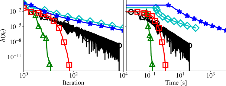
Refer to caption
Refer to caption
Figure 6: Logistic Regression: Convergence of h(𝐱t)subscript𝐱𝑡h(\mathbf{x}_{t}) and g(𝐱t)𝑔subscript𝐱𝑡g(\mathbf{x}_{t}) vs. t𝑡t and wall-clock time for the a4a LIBSVM dataset.
Refer to caption
Refer to caption
Figure 7: Logistic Regression: Convergence of h(𝐱t)subscript𝐱𝑡h(\mathbf{x}_{t}) and g(𝐱t)𝑔subscript𝐱𝑡g(\mathbf{x}_{t}) vs. t𝑡t and wall-clock time for the a8a LIBSVM dataset.

Birkhoff polytope. All applications previously considered all have in common a constraint set possessing computationally inexpensive LMOs (probability or unit simplex and 1subscript1\ell_{1} norm ball). Additionally, each vertex returned from the LMO is highly sparse with at most one non-zero element. To complement the results we consider a problem over the Birkhoff polytope, the polytope of doubly stochastic matrices, where the LMO is implemented through the Hungarian algorithm, and is not as inexpensive as in the other examples considered. We use a quadratic regularization parameter μ=100/n𝜇100𝑛\mu=100/\sqrt{n} where n𝑛n is the number of samples.

Refer to caption
Refer to caption
Figure 8: Birkhoff Polytope: Convergence of h(𝐱t)subscript𝐱𝑡h(\mathbf{x}_{t}) and g(𝐱t)𝑔subscript𝐱𝑡g(\mathbf{x}_{t}) vs. t𝑡t and wall-clock time.
Remark 4.1.

Note that Proposition 2 in Sun & Tran-Dinh [2019], which deals with the composition of generalized self-concordant functions with affine maps, does not apply to the KL divergence objective function, reproduced here for reference:

f(𝐱)=D(W𝐱,𝐲)=i=1N{𝐰i,𝐱log(𝐰i,𝐱yi)𝐰i,𝐱+yi}.𝑓𝐱𝐷𝑊𝐱𝐲superscriptsubscript𝑖1𝑁subscript𝐰𝑖𝐱subscript𝐰𝑖𝐱subscript𝑦𝑖subscript𝐰𝑖𝐱subscript𝑦𝑖f(\mathbf{x})=D(W\mathbf{x},\mathbf{y})=\sum_{i=1}^{N}\left\{\left\langle\mathbf{w}_{i},\mathbf{x}\right\rangle\log\left(\frac{\left\langle\mathbf{w}_{i},\mathbf{x}\right\rangle}{y_{i}}\right)-\left\langle\mathbf{w}_{i},\mathbf{x}\right\rangle+y_{i}\right\}.

Furthermore, the objective function is strongly convex if and only if rank(W)nrank𝑊𝑛\operatorname{rank}(W)\geq n, where n𝑛n is the dimension of the problem.

Proof.

[Sun & Tran-Dinh, 2019, Proposition 2] establishes certain conditions under which the composition of a generalized self-concordant function with an affine map results in a generalized self-concordant function. The objective is of the form:

i=1Nϕi(𝐰i,𝐱)withϕi(t)=tlog(tyi)t+yi=tlogttlogyit+yi.superscriptsubscript𝑖1𝑁subscriptitalic-ϕ𝑖subscript𝐰𝑖𝐱withsubscriptitalic-ϕ𝑖𝑡𝑡𝑡subscript𝑦𝑖𝑡subscript𝑦𝑖𝑡𝑡𝑡subscript𝑦𝑖𝑡subscript𝑦𝑖\displaystyle\sum_{i=1}^{N}\phi_{i}(\left\langle\mathbf{w}_{i},\mathbf{x}\right\rangle)\quad\text{with}\quad\phi_{i}(t)=t\log\left(\frac{t}{y_{i}}\right)-t+y_{i}=t\log t-t\log y_{i}-t+y_{i}.

Note that generalized self-concordant functions are closed under addition, and so we only focus on the individual terms in the sum. As first-order terms are (0,ν)0𝜈(0,\nu)-generalized self-concordant for any ν>0𝜈0\nu>0, then we know that the composition of these first-order terms with an affine map results in a generalized self-concordant function Sun & Tran-Dinh [2019, Proposition 2]. We therefore focus on the entropy function tlogt𝑡𝑡t\log t which is (1,4)14(1,4) generalized self-concordant. The conditions which ensure that the composition of a (M,ν)𝑀𝜈(M,\nu)-generalized self-concordant function with an affine map xAxmaps-to𝑥𝐴𝑥x\mapsto Ax results in a generalized self-concordant function requires in the case ν>3𝜈3\nu>3 that λmin(AA)>0subscript𝜆𝑚𝑖𝑛superscript𝐴top𝐴0\lambda_{min}(A^{\top}A)>0 [Sun & Tran-Dinh, 2019, Proposition 2]. In the case of the KL divergence objective, A=𝐰i𝐴superscriptsubscript𝐰𝑖topA=\mathbf{w}_{i}^{\top} and AA=𝐰i𝐰isuperscript𝐴top𝐴subscript𝐰𝑖superscriptsubscript𝐰𝑖topA^{\top}A=\mathbf{w}_{i}\mathbf{w}_{i}^{\top} is an outer product with only one positive eigenvalue, and 0 of multiplicity n1𝑛1n-1. Therefore we cannot guarantee that the function ϕi(𝐰i,𝐱)subscriptitalic-ϕ𝑖subscript𝐰𝑖𝐱\phi_{i}(\left\langle\mathbf{w}_{i},\mathbf{x}\right\rangle) is generalized self-concordant by application of Proposition 2 in Sun & Tran-Dinh [2019].

Alternatively, in order to try to show that the function is generalized self-concordant we could consider f(𝐱):=g(W𝐱)assign𝑓𝐱𝑔𝑊𝐱f(\mathbf{x}):=g(W\mathbf{x}). Assuming rank(W)nrank𝑊𝑛\operatorname{rank}(W)\geq n, then WWsuperscript𝑊top𝑊W^{\top}W is positive definite, and only the generalized self-concordance of g𝑔g is left to prove.

g(𝐳)=i=1Nϕi(𝐳i).𝑔𝐳superscriptsubscript𝑖1𝑁subscriptitalic-ϕ𝑖subscript𝐳𝑖g(\mathbf{z})=\sum_{i=1}^{N}\phi_{i}(\mathbf{z}_{i}).

Each term 𝐳ϕi(𝐳i)=ϕi(𝐞i𝐳)maps-to𝐳subscriptitalic-ϕ𝑖subscript𝐳𝑖subscriptitalic-ϕ𝑖superscriptsubscript𝐞𝑖top𝐳\mathbf{z}\mapsto\phi_{i}(\mathbf{z}_{i})=\phi_{i}(\mathbf{e}_{i}^{\top}\mathbf{z}) with 𝐞isubscript𝐞𝑖\mathbf{e}_{i} the ithsuperscript𝑖thi^{\text{th}} standard basis vector is the composition of a generalized self-concordant function composed with a rank-one affine transformation, this raises the same issues encountered in the paragraph above.

Regarding the strong-convexity of the objective function, we can express the gradient and the Hessian of the function as:

f(𝐱)=i=1N𝐰i(log𝐰i,𝐱logyi)𝑓𝐱superscriptsubscript𝑖1𝑁subscript𝐰𝑖subscript𝐰𝑖𝐱subscript𝑦𝑖\displaystyle\nabla f(\mathbf{x})=\sum_{i=1}^{N}\mathbf{w}_{i}(\log\left\langle\mathbf{w}_{i},\mathbf{x}\right\rangle-\log y_{i})
2f(𝐱)=i=1N𝐰i𝐰i𝐰i,𝐱,superscript2𝑓𝐱superscriptsubscript𝑖1𝑁subscript𝐰𝑖superscriptsubscript𝐰𝑖topsubscript𝐰𝑖𝐱\displaystyle\nabla^{2}f(\mathbf{x})=\sum_{i=1}^{N}\frac{\mathbf{w}_{i}\mathbf{w}_{i}^{\top}}{\left\langle\mathbf{w}_{i},\mathbf{x}\right\rangle},

which is the sum of N𝑁N outer products, each corresponding to a single eigenvector 𝐰isubscript𝐰𝑖\mathbf{w}_{i}. If rank(W)nrank𝑊𝑛\operatorname{rank}(W)\geq n, the Hessian is definite positive and the objective is strongly convex. Otherwise, it possesses zero as an eigenvalue regardless of 𝐱𝐱\mathbf{x}, and the function Hessian is positive semi-definite. ∎

Strong convexity parameter for the LLOO.

The LLOO procedure explicitly requires a strong convexity parameter σfsubscript𝜎𝑓\sigma_{f} of the objective function, an underestimator of λmin(2f(𝐱))subscript𝜆𝑚𝑖𝑛superscript2𝑓𝐱\lambda_{min}(\nabla^{2}f(\mathbf{x})) over 𝒳𝒳\mathcal{X}. For the portfolio optimization problem, the Hessian is a sum of rank-one terms:

2f(𝐱)=t𝐫t𝐫t𝐫t,𝐱.superscript2𝑓𝐱subscript𝑡subscript𝐫𝑡superscriptsubscript𝐫𝑡topsubscript𝐫𝑡𝐱\displaystyle\nabla^{2}f(\mathbf{x})=\sum_{t}\frac{\mathbf{r}_{t}\mathbf{r}_{t}^{\top}}{\left\langle\mathbf{r}_{t},\mathbf{x}\right\rangle}.

The only non-zero eigenvalue associated with each t𝑡t term is bounded below over 𝒳𝒳\mathcal{X} by:

𝐫t2max𝐱𝒳𝐫t,𝐱2=𝐫t2max{max𝐱𝒳𝐫t,𝐱,min𝐱𝒳𝐫t,𝐱}2.\displaystyle\frac{\left\|\mathbf{r}_{t}\right\|^{2}}{\max_{\mathbf{x}\in\mathcal{X}}\left\langle\mathbf{r}_{t},\mathbf{x}\right\rangle^{2}}=\frac{\left\|\mathbf{r}_{t}\right\|^{2}}{\max\{\max_{\mathbf{x}\in\mathcal{X}}\left\langle\mathbf{r}_{t},\mathbf{x}\right\rangle,-\min_{\mathbf{x}\in\mathcal{X}}\left\langle\mathbf{r}_{t},\mathbf{x}\right\rangle\}^{2}}.

The denominator can be solved by two calls to the LMO, and we will denote it by βtsubscript𝛽𝑡\beta_{t} for the tthsuperscript𝑡tht^{\text{th}} term. Each summation term contributes positively to one of the eigenvalues of the Hessian matrix, an underestimator of the the strong convexity parameter is then given by:

λmin(t𝐫t𝐫tβt).subscript𝜆𝑚𝑖𝑛subscript𝑡subscript𝐫𝑡superscriptsubscript𝐫𝑡topsubscript𝛽𝑡\displaystyle\lambda_{min}\left(\sum_{t}\frac{\mathbf{r}_{t}\mathbf{r}_{t}^{\top}}{\beta_{t}}\right).

The second-order method GSC-FW has been implemented with an in-place Hessian matrix updated at each iteration, following the implementation of Dvurechensky et al. [2022]. The Hessian computation nonetheless adds significant cost in the runtime of each iteration, even if the local norm and other quadratic expressions 2f(𝐱)𝐲,𝐳superscript2𝑓𝐱𝐲𝐳\left\langle\nabla^{2}f(\mathbf{x})\mathbf{y},\mathbf{z}\right\rangle can be computed allocation-free. A potential improvement for future work would be to represent Hessian matrices as functional linear operators mapping any 𝐲𝐲\mathbf{y} to 2f(𝐱)𝐲superscript2𝑓𝐱𝐲\nabla^{2}f(\mathbf{x})\mathbf{y}.

Monotonic step size: the numerical case.

The computational experiments highlighted that the Monotonic Frank-Wolfe performs well in terms of iteration count and time against other Frank-Wolfe and Away-step Frank-Wolfe variants. Another advantage of a simple step size computation procedure is its numerical stability. On some instances, an ill-conditioned gradient can lead to a plateau of the primal and/or dual progress. Even worse, some step-size strategies do not guarantee monotonicity and can result in the primal value increasing over some iterations. The numerical issue that causes this phenomenon is illustrated by running the methods of the FrankWolfe.jl package over the same instance using 646464-bits floating-point numbers and Julia BigFloat types (which support arithmetic in arbitrary precision to remove numerical issues).
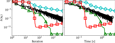
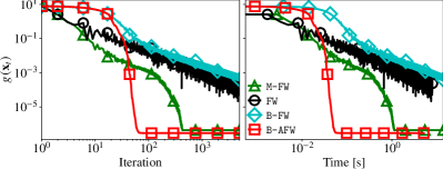
Refer to caption
(a)
Refer to caption
(b)
Figure 9: Ill-conditioned portfolio optimization problem solved using floating-point arithmetic.
Refer to caption
(a)
Refer to caption
(b)
Figure 10: Ill-conditioned portfolio optimization problem solved using arbitrary precision.

In Figure 9, we observe a plateau of the dual gap for both M-FW and B-AFW. The primal value however worsens after the iteration where B-AFW reaches its dual gap plateau. In contrast, M-FW reaches a plateau in both primal and dual gap at a certain iteration. Note that the primal value at the point where the plateau is hit is already below εfloat64subscript𝜀float64\sqrt{\varepsilon_{\text{float}64}}, the square root of the machine precision. The same instance and methods operating in arbitrary precision arithmetic are presented Figure 10. Instead of reaching a plateau or deteriorating, B-AFW closes the dual gap tolerance and terminates before other methods. Although this observation (made on several instances of the portfolio optimization problem) only impacts ill-conditioned problems, it suggests M-FW may be a good candidate for a numerically robust default implementation of Frank-Wolfe algorithms.

Function domain in the constraints

One of the arguments used to motivate the construction of FW algorithms for standard and generalized self-concordant minimization in prior work is the difficulty of handling objective functions with implicitly defined domains. We make several observations that highlight the relevance of this issue and justify the assumption of the availability of a Domain Oracle for dom(f)dom𝑓\mathrm{dom}(f). In the portfolio optimization example, all revenue vectors are assumed positive, 𝐫t++nsubscript𝐫𝑡subscriptsuperscript𝑛absent\mathbf{r}_{t}\in\mathbb{R}^{n}_{++} and 𝐱Δn𝐱subscriptΔ𝑛\mathbf{x}\in\Delta_{n}, it follows that all feasible points lie in dom(f)dom𝑓\mathrm{dom}(f). More generally ,for the logarithm of an affine function, verifying that a candidate 𝐱𝐱\mathbf{x} lies in dom(f)dom𝑓\mathrm{dom}(f) consists of a single affine transformation and element-wise comparison A𝐱+𝐛>++m𝐴𝐱𝐛superscriptsubscriptabsent𝑚A\mathbf{x}+\mathbf{b}>\mathbb{R}_{++}^{m}.

In the inverse covariance estimation problem, the information on dom(f)dom𝑓\mathrm{dom}(f) can be added to the constraints by imposing mat(𝐱)𝕊+nmat𝐱superscriptsubscript𝕊𝑛\text{mat}(\mathbf{x})\in\mathbb{S}_{+}^{n}, yielding a semi-definite optimization problem. The domain oracle consists of the computation of the smallest eigenvalue, which needs to be positive.

We can also modify the feasible region of the signal retrieval application using the KL divergence, resulting in a new feasible region 𝒳superscript𝒳\mathcal{X}^{\prime} so that Int(𝒳)dom(f)Intsuperscript𝒳dom𝑓\operatorname{\mathrm{Int}}\left(\mathcal{X}^{\prime}\right)\subset\mathrm{dom}(f). The objective is of the form:

f(θ)=i𝐰i,θlog(𝐰i,θyi)𝐰i,θ𝑓𝜃subscript𝑖subscript𝐰𝑖𝜃subscript𝐰𝑖𝜃subscript𝑦𝑖subscript𝐰𝑖𝜃f(\theta)=\sum_{i}\langle\mathbf{w}_{i},\theta\rangle\log\left(\frac{\langle\mathbf{w}_{i},\theta\rangle}{y_{i}}\right)-\langle\mathbf{w}_{i},\theta\rangle

where the data W𝑊W and y𝑦y are assumed to be entrywise positive, thus dom(f)={x+n,x0}dom𝑓formulae-sequence𝑥subscriptsuperscript𝑛𝑥0\mathrm{dom}(f)=\{x\in\mathbb{R}^{n}_{+},x\neq 0\}. Therefore we can define the set 𝒳superscript𝒳\mathcal{X}^{\prime} as the unit simplex. The domain of each function involved in the sum in f𝑓f has an open domain (0,+)0(0,+\infty).

However, the positivity assumption on all these components could be relaxed. Without the positivity assumption on W𝑊W, the Domain Oracle would consist of verifying:

𝐰i,θ>0i.subscript𝐰𝑖𝜃0for-all𝑖\langle\mathbf{w}_{i},\theta\rangle>0\,\,\forall i. (4.1)

This verification can however be simplified by a preprocessing step if the number of data points is large by finding the minimal set of supporting hyperplanes in the polyhedral cone (4.1), which we can find by solving the following linear problem:

maxτ,θsubscript𝜏𝜃\displaystyle\max_{\tau,\theta}\,\, τ𝜏\displaystyle\tau (4.2a)
s.t. τ𝐰i,θi(λi)𝜏subscript𝐰𝑖𝜃for-all𝑖subscript𝜆𝑖\displaystyle\tau\leq\langle\mathbf{w}_{i},\theta\rangle\,\,\forall i\,\,\,\,(\lambda_{i}) (4.2b)
θ1R,subscriptnorm𝜃1𝑅\displaystyle\left\|\theta\right\|_{1}\leq R, (4.2c)

where λisubscript𝜆𝑖\lambda_{i} is the dual variable associated with the ithsuperscript𝑖thi^{\text{th}} inner product constraint. If the optimal solution of Problem (4.2a) is 00, the original problem is infeasible and the cone defined by (4.1) is empty. Otherwise the optimal θ𝜃\theta will lie in the intersection of the closure of the polyhedral cone and the 1subscript1\ell_{1} norm ball. Furthermore, the support of λ𝜆\lambda provides us with the non-redundant inequalities of the cone. Let W^^𝑊\hat{W} be the matrix formed with the rows 𝐰isubscript𝐰𝑖\mathbf{w}_{i} such that λi>0subscript𝜆𝑖0\lambda_{i}>0, then the Domain Oracle can be simplified to the verification that W^θ++n^𝑊𝜃subscriptsuperscript𝑛absent\hat{W}\theta\in\mathbb{R}^{n}_{++}. The Distance Weighted Discrimination (DWT) model also considered in Dvurechensky et al. [2022] was initially presented in Marron et al. [2007], the denominator of each sum element ξisubscript𝜉𝑖\xi_{i} is initially constrained to be nonnegative, which makes Int(𝒳)dom(f)Int𝒳dom𝑓\operatorname{\mathrm{Int}}\left(\mathcal{X}\right)\subseteq\mathrm{dom}(f) hold. Even without this additional constraint, the nonnegativity of all ξisubscript𝜉𝑖\xi_{i} can be ensured with a minimum set of linear constraints in a fashion similar to the signal retrieval application, thus simplifying the Domain Oracle.

A stateless simple step variant.

The simple step-size strategy presented in Algorithm 2 ensures monotonicity and domain-respecting iterates by maintaining a “memory” ϕtsubscriptitalic-ϕ𝑡\phi_{t} which is the number of performed halvings. The number of halvings to reach an accepted step is bounded, but the corresponding factor 2ϕtsuperscript2subscriptitalic-ϕ𝑡2^{\phi_{t}} is carried over in all following iterations, which may slow down progress. We propose an alternative step size that still ensures the monotonicity and domain-preserving properties, but does not carry over information from one iteration to the next.

Algorithm 7 Stateless Monotonic Frank-Wolfe
1:Point 𝐱0𝒳dom(f)subscript𝐱0𝒳dom𝑓\mathbf{x}_{0}\in\mathcal{X}\cap\mathrm{dom}(f), function f𝑓f
2:Iterates 𝐱1,𝒳subscript𝐱1𝒳\mathbf{x}_{1},\dotsc\in\mathcal{X}  
3:for t=0𝑡0t=0 to \dotsc do
4:     𝐯targmin𝐯𝒳f(𝐱t),𝐯subscript𝐯𝑡subscriptargmin𝐯𝒳𝑓subscript𝐱𝑡𝐯\mathbf{v}_{t}\leftarrow\operatorname*{argmin}_{\mathbf{v}\in\mathcal{X}}\left\langle\nabla f(\mathbf{x}_{t}),\mathbf{v}\right\rangle
5:     γt2/(t+2)subscript𝛾𝑡2𝑡2\gamma_{t}\leftarrow 2/(t+2)
6:     𝐱t+1𝐱t+γt(𝐯t𝐱t)subscript𝐱𝑡1subscript𝐱𝑡subscript𝛾𝑡subscript𝐯𝑡subscript𝐱𝑡\mathbf{x}_{t+1}\leftarrow\mathbf{x}_{t}+\gamma_{t}(\mathbf{v}_{t}-\mathbf{x}_{t})
7:     while 𝐱t+1dom(f)subscript𝐱𝑡1dom𝑓\mathbf{x}_{t+1}\notin\mathrm{dom}(f) or f(𝐱t+1)>f(𝐱t)𝑓subscript𝐱𝑡1𝑓subscript𝐱𝑡f(\mathbf{x}_{t+1})>f(\mathbf{x}_{t}) do
8:         γtγt/2subscript𝛾𝑡subscript𝛾𝑡2\gamma_{t}\leftarrow\gamma_{t}/2
9:         𝐱t+1𝐱t+γt(𝐯t𝐱t)subscript𝐱𝑡1subscript𝐱𝑡subscript𝛾𝑡subscript𝐯𝑡subscript𝐱𝑡\mathbf{x}_{t+1}\leftarrow\mathbf{x}_{t}+\gamma_{t}(\mathbf{v}_{t}-\mathbf{x}_{t})      

Note that Algorithm 7, presented above, is stateless since it is equivalent to Algorithm 2 with ϕtsubscriptitalic-ϕ𝑡\phi_{t} reset to zero between every outer iteration. This resetting step also implies that the per-iteration convergence rate of the stateless step is at least as good as the simple step, at the potential cost of a bounded number of halvings, with associated ZOO and DOO calls at each iteration. Finally, we point out that the stateless step-size strategy can be viewed as a particular instance of a backtracking line search where the initial step size estimate is the agnostic step size 2/(t+2)2𝑡22/(t+2).

We compare the two strategies on a random and badly conditioned problem with objective function:

xQx+b,x+μφ+(x)superscript𝑥top𝑄𝑥𝑏𝑥𝜇subscript𝜑subscript𝑥x^{\top}Qx+\left\langle b,x\right\rangle+\mu\varphi_{\mathbb{R}_{+}}(x)

where Q𝑄Q is a symmetric positive definite matrix with log-normally distributed eigenvalues and φ+()subscript𝜑subscript\varphi_{\mathbb{R}_{+}}(\cdot) is the log-barrier function of the positive orthant. We optimize instances of this function over the 1subscript1\ell_{1}-norm ball in dimension 303030 and 100010001000. The results are shown in Figure 11 and 12 for n=30𝑛30n=30 and n=1000𝑛1000n=1000, respectively. On both of these instances, the simple step progress is slowed down or even seems stalled in comparison to the stateless version because a lot of halving steps were done in the early iterations for the simple step size, which penalizes progress over the whole run. The stateless step-size does not suffer from this problem, however, because the halvings have to be performed at multiple iterations when using the stateless step-size strategy, the per iteration cost of the stateless step-size is about three times that of the simple step-size. Future work will consider additional restart conditions, not only on ϕtsubscriptitalic-ϕ𝑡\phi_{t} of Algorithm 2, but also on the base step-size strategy employed, similar to Kerdreux et al. [2019].
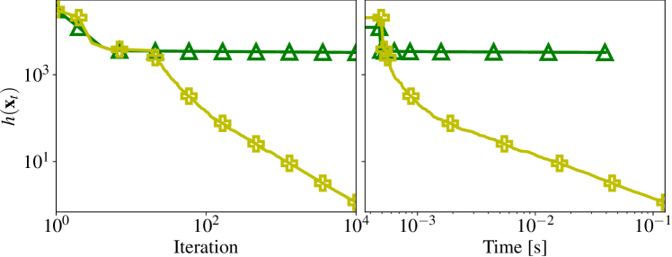
Refer to caption
Refer to caption
Figure 11: Stateless step-size: Comparison of the stateless and simple steps on badly conditioned problems with n=30𝑛30n=30.
Refer to caption
Refer to caption
Figure 12: Stateless step-size: Comparison of the stateless and simple steps on badly conditioned problems with n=1000𝑛1000n=1000.

Conclusion

We present in this paper a simple Frank-Wolfe variant that utilizes the open-loop step size strategy γt=2/(t+2)subscript𝛾𝑡2𝑡2\gamma_{t}=2/(t+2) to obtain a 𝒪(1/t)𝒪1𝑡\mathcal{O}(1/t) convergence rate for generalized self-concordant functions in terms of primal gap and Frank-Wolfe gap, where t𝑡t is the iteration count. This algorithm neither requires second-order information, nor line searches. Moreover, the simple nature of the algorithm allows us to precisely bound the number of zeroth-order oracle, first-order oracle, domain oracle and linear optimization oracle calls that are needed to obtain a target accuracy in primal gap or Frank-Wolfe gap. This is in contrast to other existing bounds, which are only informative with respect to first-order and linear optimization oracle calls, and hide the zeroth-order and domain oracle complexity in line search procedures.

We also show improved convergence rates for several variants in various cases of interest and prove that the Away-step Frank-Wolfe algorithm [Wolfe, 1970, Lacoste-Julien & Jaggi, 2015] coupled with the backtracking line search of Pedregosa et al. [2020] can achieve linear convergence rates over polytopes when minimizing generalized self-concordant functions.

Acknowledgements

Research reported in this paper was partially supported through the Research Campus Modal funded by the German Federal Ministry of Education and Research (fund numbers 05M14ZAM,05M20ZBM) and the Deutsche Forschungsgemeinschaft (DFG) through the DFG Cluster of Excellence MATH+. We would like to thank the anonymous reviewers for their suggestions and comments.

References

  • Bach [2010] Bach, F. Self-concordant analysis for logistic regression. Electronic Journal of Statistics, 4:384–414, 2010.
  • Besançon et al. [2022] Besançon, M., Carderera, A., and Pokutta, S. FrankWolfe.jl: a high-performance and flexible toolbox for Frank-Wolfe algorithms and conditional gradients. INFORMS Journal on Computing, 34(5):2611–2620, 2022.
  • Carderera et al. [2021] Carderera, A., Besançon, M., and Pokutta, S. Frank-Wolfe for Generalized Self-Concordant Functions - Problem Instances, May 2021. URL https://doi.org/10.5281/zenodo.4836009.
  • Csiszar [1991] Csiszar, I. Why least squares and maximum entropy? An axiomatic approach to inference for linear inverse problems. The annals of statistics, 19(4):2032–2066, 1991.
  • Diakonikolas et al. [2020] Diakonikolas, J., Carderera, A., and Pokutta, S. Locally accelerated conditional gradients. In Proceedings of the 23th International Conference on Artificial Intelligence and Statistics, pp.  1737–1747. PMLR, 2020.
  • Dvurechensky et al. [2020] Dvurechensky, P., Ostroukhov, P., Safin, K., Shtern, S., and Staudigl, M. Self-concordant analysis of Frank-Wolfe algorithms. In Proceedings of the 37th International Conference on Machine Learning, pp.  2814–2824. PMLR, 2020.
  • Dvurechensky et al. [2022] Dvurechensky, P., Safin, K., Shtern, S., and Staudigl, M. Generalized self-concordant analysis of Frank–Wolfe algorithms. Mathematical Programming, pp.  1–69, 2022.
  • Frank & Wolfe [1956] Frank, M. and Wolfe, P. An algorithm for quadratic programming. Naval research logistics quarterly, 3(1-2):95–110, 1956.
  • Garber & Hazan [2016] Garber, D. and Hazan, E. A linearly convergent variant of the conditional gradient algorithm under strong convexity, with applications to online and stochastic optimization. SIAM Journal on Optimization, 26(3):1493–1528, 2016.
  • Guélat & Marcotte [1986] Guélat, J. and Marcotte, P. Some comments on Wolfe’s ‘away step’. Mathematical Programming, 35(1):110–119, 1986.
  • Jaggi [2013] Jaggi, M. Revisiting Frank-Wolfe: Projection-free sparse convex optimization. In Proceedings of the 30th International Conference on Machine Learning, pp.  427–435. PMLR, 2013.
  • Kerdreux et al. [2019] Kerdreux, T., d’Aspremont, A., and Pokutta, S. Restarting Frank-Wolfe. In Proceedings of the 22nd International Conference on Artificial Intelligence and Statistics, pp.  1275–1283. PMLR, 2019.
  • Kerdreux et al. [2021] Kerdreux, T., d’Aspremont, A., and Pokutta, S. Projection-free optimization on uniformly convex sets. In Proceedings of the 24th International Conference on Artificial Intelligence and Statistics, pp.  19–27. PMLR, 2021.
  • Krishnan et al. [2015] Krishnan, R. G., Lacoste-Julien, S., and Sontag, D. Barrier Frank-Wolfe for Marginal Inference. In Proceedings of the 28th Conference in Neural Information Processing Systems. PMLR, 2015.
  • Lacoste-Julien & Jaggi [2015] Lacoste-Julien, S. and Jaggi, M. On the global linear convergence of Frank-Wolfe optimization variants. In Proceedings of the 29th Conference on Neural Information Processing Systems, pp.  566–575. PMLR, 2015.
  • Levitin & Polyak [1966] Levitin, E. S. and Polyak, B. T. Constrained minimization methods. USSR Computational Mathematics and Mathematical Physics, 6(5):1–50, 1966.
  • Liu et al. [2020] Liu, D., Cevher, V., and Tran-Dinh, Q. A newton frank–wolfe method for constrained self-concordant minimization. Journal of Global Optimization, pp.  1–27, 2020.
  • Marron et al. [2007] Marron, J. S., Todd, M. J., and Ahn, J. Distance-weighted discrimination. Journal of the American Statistical Association, 102(480):1267–1271, 2007.
  • Marteau-Ferey et al. [2019] Marteau-Ferey, U., Ostrovskii, D., Bach, F., and Rudi, A. Beyond least-squares: Fast rates for regularized empirical risk minimization through self-concordance. In Proceedings of the 32nd Conference on Learning Theory, pp.  2294–2340. PMLR, 2019.
  • Nesterov [2013] Nesterov, Y. Gradient methods for minimizing composite functions. Mathematical Programming, 140(1):125–161, 2013.
  • Nesterov [2018] Nesterov, Y. Lectures on convex optimization, volume 137. Springer, 2018.
  • Nesterov & Nemirovskii [1994] Nesterov, Y. and Nemirovskii, A. Interior-point polynomial algorithms in convex programming. SIAM, 1994.
  • Odor et al. [2016] Odor, G., Li, Y.-H., Yurtsever, A., Hsieh, Y.-P., Tran-Dinh, Q., El Halabi, M., and Cevher, V. Frank-wolfe works for non-lipschitz continuous gradient objectives: scalable poisson phase retrieval. In 2016 IEEE International Conference on Acoustics, Speech and Signal Processing (ICASSP), pp.  6230–6234. Ieee, 2016.
  • Ostrovskii & Bach [2021] Ostrovskii, D. M. and Bach, F. Finite-sample analysis of M-estimators using self-concordance. Electronic Journal of Statistics, 15(1):326–391, 2021.
  • Pedregosa et al. [2020] Pedregosa, F., Negiar, G., Askari, A., and Jaggi, M. Linearly convergent Frank–Wolfe with backtracking line-search. In Proceedings of the 23rd International Conference on Artificial Intelligence and Statistics. PMLR, 2020.
  • Rothvoß [2017] Rothvoß, T. The matching polytope has exponential extension complexity. Journal of the ACM (JACM), 64(6):1–19, 2017.
  • Sun & Tran-Dinh [2019] Sun, T. and Tran-Dinh, Q. Generalized self-concordant functions: a recipe for Newton-type methods. Mathematical Programming, 178(1):145–213, 2019.
  • Temlyakov [2015] Temlyakov, V. Greedy approximation in convex optimization. Constructive Approximation, 41(2):269–296, 2015.
  • Tran-Dinh et al. [2015] Tran-Dinh, Q., Li, Y.-H., and Cevher, V. Composite convex minimization involving self-concordant-like cost functions. In Modelling, Computation and Optimization in Information Systems and Management Sciences, pp.  155–168. Springer, 2015.
  • Tsuji et al. [2022] Tsuji, K. K., Tanaka, K., and Pokutta, S. Pairwise conditional gradients without swap steps and sparser kernel herding. In International Conference on Machine Learning, pp.  21864–21883. PMLR, 2022.
  • Wolfe [1970] Wolfe, P. Convergence theory in nonlinear programming. In Integer and Nonlinear Programming, pp.  1–36. North-Holland, Amsterdam, 1970.
  • Zhao & Freund [2023] Zhao, R. and Freund, R. M. Analysis of the Frank–Wolfe method for convex composite optimization involving a logarithmically-homogeneous barrier. Mathematical Programming, 199(1-2):123–163, 2023.