Conic Blackwell Algorithm: Parameter-Free Convex-Concave Saddle-Point Solving

Julien Grand-Clément
ISOM Department & Hi!Paris
HEC Paris
grand-clement@hec.fr
&Christian Kroer
IEOR Department
Columbia University
christian.kroer@columbia.edu
Abstract

We develop new parameter-free and scale-free algorithms for solving convex-concave saddle-point problems. Our results are based on a new simple regret minimizer, the Conic Blackwell Algorithm+ (CBA+), which attains O(1/T)𝑂1𝑇O(1/\sqrt{T}) average regret. Intuitively, our approach generalizes to other decision sets of interest ideas from the Counterfactual Regret minimization (CFR+) algorithm, which has very strong practical performance for solving sequential games on simplexes. We show how to implement CBA+ for the simplex, psubscript𝑝\ell_{p} norm balls, and ellipsoidal confidence regions in the simplex, and we present numerical experiments for solving matrix games and distributionally robust optimization problems. Our empirical results show that CBA+ is a simple algorithm that outperforms state-of-the-art methods on synthetic data and real data instances, without the need for any choice of step sizes or other algorithmic parameters.

1 Introduction

We are interested in solving saddle-point problems (SPPs) of the form

min𝒙𝒳max𝒚𝒴F(𝒙,𝒚),subscript𝒙𝒳subscript𝒚𝒴𝐹𝒙𝒚\displaystyle\min_{\bm{x}\in\mathcal{X}}\max_{\bm{y}\in\mathcal{Y}}F(\bm{x},\bm{y}), (1)

where 𝒳n,𝒴mformulae-sequence𝒳superscript𝑛𝒴superscript𝑚\mathcal{X}\subset\mathbb{R}^{n},\mathcal{Y}\subset\mathbb{R}^{m} are convex, compact sets, and F:𝒳×𝒴:𝐹𝒳𝒴F:\mathcal{X}\times\mathcal{Y}\rightarrow\mathbb{R} is a subdifferentiable convex-concave function. Convex-concave SPPs arise in a number of practical problems. For example, the problem of computing a Nash equilibrium of a zero-sum games can be formulated as a convex-concave SPP, and this is the foundation of most methods for solving sequential zero-sum games (von Stengel, 1996; Zinkevich et al., 2007; Tammelin et al., 2015; Kroer et al., 2020). They also arise in imaging (Chambolle and Pock, 2011), subscript\ell_{\infty}-regression (Sidford and Tian, 2018), Markov Decision Processes (Iyengar, 2005; Wiesemann et al., 2013; Sidford and Tian, 2018), and in distributionally robust optimization, where the max term represents the distributional uncertainty (Namkoong and Duchi, 2016; Ben-Tal et al., 2015). In this paper we propose efficient, parameter-free algorithms for solving (1) in many settings, i.e., algorithms that do not require any tuning or choices of step sizes.

Repeated game framework

One way to solve convex-concave SPPs is by viewing the SPP as a repeated game between two players, where each step t𝑡t consists of one player choosing 𝒙t𝒳subscript𝒙𝑡𝒳\bm{x}_{t}\in\mathcal{X}, the other player choosing 𝒚t𝒴subscript𝒚𝑡𝒴\bm{y}_{t}\in\mathcal{Y}, and then the players observe the payoff F(𝒙t,𝒚t)𝐹subscript𝒙𝑡subscript𝒚𝑡F(\bm{x}_{t},\bm{y}_{t}). If each player employs a regret-minimization algorithm, then a well-known folk theorem says that the uniform average strategy generated by two regret minimizers repeatedly playing an SPP against each other converges to a solution to the SPP. We will call this the “repeated game framework” (see Section 2). There are already well-known algorithms for instantiating the above repeated game framework for (1). For example, one can employ the online mirror descent (OMD) algorithm, which generates iterates as follows for the first player (and similarly for the second player):

𝒙t+1=argmin𝒙𝒳η𝒇t,𝒙+D(𝒙𝒙t),subscript𝒙𝑡1subscriptargmin𝒙𝒳𝜂subscript𝒇𝑡𝒙𝐷conditional𝒙subscript𝒙𝑡\displaystyle\bm{x}_{t+1}=\operatorname*{arg\,min}_{\bm{x}\in\mathcal{X}}\langle\eta\bm{f}_{t},\bm{x}\rangle+D(\bm{x}\|\bm{x}_{t}), (2)

where 𝒇t𝒙F(𝒙t,𝒚t)subscript𝒇𝑡subscript𝒙𝐹subscript𝒙𝑡subscript𝒚𝑡\bm{f}_{t}\in\partial_{\bm{x}}F(\bm{x}_{t},\bm{y}_{t}) (𝒙subscript𝒙\partial_{\bm{x}} denotes here the set of subgradients as regards the variable 𝒙𝒙\bm{x}), D()D(\cdot\|\cdot) is a Bregman divergence which measures distance between pairs of points, and η>0𝜂0\eta>0 is an appropriate step size. By choosing D𝐷D appropriately for 𝒳𝒳\mathcal{X}, the update step (2) becomes efficient, and one can achieve an overall regret on the order of O(T)𝑂𝑇O(\sqrt{T}) after T𝑇T iterations. This regret can be achieved either by choosing a fixed step size η=α/LT𝜂𝛼𝐿𝑇\eta=\alpha/L\sqrt{T}, where an upper bound L𝐿L on the norms of the subgradients visited (𝒈t)t0subscriptsubscript𝒈𝑡𝑡0\left(\bm{g}_{t}\right)_{t\geq 0}, or by choosing adaptive step sizes ηt=α/tsubscript𝜂𝑡𝛼𝑡\eta_{t}=\alpha/\sqrt{t}, for α>0𝛼0\alpha>0. This is problematic, as 1) the upper bound L𝐿L may be hard to obtain in many applications and may be too conservative in practice, and 2) adequately tuning the parameter α𝛼\alpha can be time- and resource-consuming, and even practically infeasible for very large instances, since we won’t know if the step size will cause a divergence until late in the optimization process. This is not just a theoretical issue, as we highlight in our numerical experiments (Section 4) and in the appendices (Appendices F). Similar results and challenges hold for the popular follow the regularized leader (FTRL) algorithm (see Appendix F).

The above issues can be circumvented by employing adaptive variants of OMD or FTRL, which lead to parameter- and scale-free algorithms that estimate the parameters through the observed subgradients, e.g., AdaHedge for the simplex setting (De Rooij et al., 2014) or AdaFTRL for general compact convex decisions sets (Orabona and Pál, 2015). Yet these adaptive variants have not seen practical adoption in large-sale game-solving, where regret-matching variants are preferred (see the next paragraph). As we show in our experiments, adaptive variants of OMD and FTRL perform much worse than our proposed algorithms. While these adaptive algorithms are referred to as parameter-free, this is only true in the sense that they are able to learn the necessary parameters. Our algorithm is parameter-free in the stronger sense that there are no parameters that even require learning. Formalizing this difference may be one interesting avenue for explaining the performance discrepancy on saddle-point problems.

Regret Matching

In this paper, we introduce alternative regret-minimization schemes for instantiating the above framework. Our work is motivated by recent advances on solving large-scale zero-sum sequential games. In the zero-sum sequential game setting, 𝒳𝒳\mathcal{X} and 𝒴𝒴\mathcal{Y} are simplexes, the objective function becomes F(𝒙,𝒚)=𝒙,𝑨𝒚𝐹𝒙𝒚𝒙𝑨𝒚F(\bm{x},\bm{y})=\langle\bm{x},\bm{Ay}\rangle, and thus (1) reduces to a bilinear SPP. Based on this bilinear SPP formulation, the best practical methods for solving large-scale sequential games use the repeated game framework, where each player minimizes regret via some variant of counterfactual regret minimization (CFR, (Zinkevich et al., 2007)). Variants of CFR were used in every recent poker AI challenge, where poker AIs beat human poker players (Bowling et al., 2015; Moravčík et al., 2017; Brown and Sandholm, 2018, 2019). The CFR framework itself is a decomposition of the overall regret of the bilinear SPP into local regrets at each decision point in a sequential game (Farina et al., 2019a). The key to the practical performance of CFR-based algorithms seems to be three ingredients (beyond the CFR decomposition itself): (1) a particular regret minimizer called regret matching+ (RM+(Tammelin et al., 2015) which is employed at each decision point, (2) aggressive iterate averaging schemes that put greater weight on recent iterates (e.g. linear averaging, which weights iterate at period t𝑡t by 2t/T(T+1)2𝑡𝑇𝑇12t/T(T+1)), and (3) an alternation scheme where the updates of the repeated game framework are performed in an asymmetric fashion. The CFR framework itself is specific to sequential bilinear games on simplexes, but these last three ingredients could potentially be generalized to other problems of the form (1). That is the starting point of the present paper.

The most challenging aspect of generalizing the above ingredients is that RM+ is specifically designed for minimizing regret over a simplex. However, many problems of the form (1) have convex sets 𝒳,𝒴𝒳𝒴\mathcal{X},\mathcal{Y} that are not simplexes, e.g., box constraints or norm-balls for distributionally robust optimization (Ben-Tal et al., 2015). In principle, regret matching arises from a general theory called Blackwell approachability (Blackwell, 1956; Hart and Mas-Colell, 2000), and similar constructions can be envisioned for other convex sets. However, in practice the literature has only focused on developing concrete implementable instantiations of Blackwell approachability for simplexes. A notable deviation from this is the work of Abernethy et al. (2011), who showed a general reduction between regret minimization over general convex compact sets and Blackwell approachability. However, their general reduction still does not yield a practically implementable algorithm: among other things, their reduction relies on certain black-box projections that are not always efficient. We show how to implement these necessary projections for the setting where 𝒳𝒳\mathcal{X} and 𝒴𝒴\mathcal{Y} are simplexes, psubscript𝑝\ell_{p} balls, and intersections of the 2subscript2\ell_{2} ball with a hyperplane (with a focus on the case where an 2subscript2\ell_{2} ball is intersected with a simplex, which arises naturally as confidence regions). This yields an algorithm which we will refer to as the conic Blackwell algorithm (CBA), which is similar in spirit to the regret matching algorithm, but crucially generalizes to other decision sets. Motivated by the practical performance of RM+, we construct a variant of CBA which uses a thresholding operation similar to the one employed by RM+. We call this algorithm CBA+.

Our contributions

We introduce CBA+, a parameter-free algorithm which achieves O(T)𝑂𝑇O(\sqrt{T}) regret in the worst-case and generalizes the strong performances of RM+ for bilinear, simplex saddle-points solving to other more general settings. A major selling point for CBA+ is that it does not require any step size choices. Instead, the algorithm implicitly adjusts to the structure of the domains and losses by being instantiations of Blackwell’s approachability algorithm. After developing the CBA+ algorithm, we then develop analogues of another crucial components for large-scale game solving. In particular, we prove a generalization of the folk theorem for the repeated game framework for solving (1), which allows us to incorporate polynomial averaging schemes such as linear averaging. We then show that CBA+ is compatible with linear averaging on the iterates. This mirrors the case of RM and RM+, where only RM+ is compatible with linear averaging on the iterates. We also show that both CBA and CBA+ are compatible with polynomial averaging when simultaneously performed on the regrets and the iterates. Combining all these ingredients, we arrive at a new class of algorithms for solving convex-concave SPPs. As long as efficient projection operations can be performed (which we show for several practical domains, including the simplex, psubscript𝑝\ell_{p} balls and confidence regions in the simplex), one can apply the repeated game framework on (1), where one can use either CBA or CBA+ as a regret minimizer for 𝒳𝒳\mathcal{X} and 𝒴𝒴\mathcal{Y} along with polynomial averaging on the generated iterates to solve (1) at a rate of O(1/T)𝑂1𝑇O\left(1/\sqrt{T}\right).

We highlight the practical efficacy of our algorithmic framework on several domains. First, we solve two-player zero-sum matrix games and extensive-form games, where RM+ regret minimizer combined with linear averaging and alternation, and CFR+, lead to very strong practical algorithms (Tammelin et al., 2015). We find that CBA+ combined with linear averaging and alternation leads to a comparable performance in terms of the iteration complexity, and may even slightly outperform RM+ and CFR+. On this simplex setting, we also find that CBA+ outperforms both AdaHedge and AdaFTRL. Second, we apply our approach to a setting where RM+ and CFR+ do not apply: distributionally robust empirical risk minimization (DR-ERM) problems. Across two classes of synthetic problems and four real data sets, we find that our algorithm based on CBA+ performs orders of magnitude better than online mirror descent and FTRL, as well as their optimistic variants, when using their theoretically-correct fixed step sizes. Even when considering adaptive step sizes, or fixed step sizes that are up to 10,0001000010,000 larger than those predicted by theory, our CBA+ algorithm performs better, with only a few cases of comparable performance (at step sizes that lead to divergence for some of the other non-parameter free methods). The fast practical performance of our algorithm, combined with its simplicity and the total lack of step sizes or parameters tuning, suggests that it should be seriously considered as a practical approach for solving convex-concave SPPs in various settings.

Finally, we make a brief note on accelerated methods. Our algorithms have a rate of convergence towards a saddle point of O(1/T)𝑂1𝑇O(1/\sqrt{T}), similar to OMD and FTRL. In theory, it is possible to obtain a faster O(1/T)𝑂1𝑇O\left(1/T\right) rate of convergence when F𝐹F is differentiable with Lipschitz gradients, for example via mirror prox (Nemirovski, 2004) or other primal-dual algorithms (Chambolle and Pock, 2016). However, our experimental results show that CBA+ is faster than optimistic variants of FTRL and OMD (Syrgkanis et al., 2015), the latter being almost identical to the mirror prox algorithm, and both achieving O(1/T)𝑂1𝑇O(1/T) rate of convergence. A similar conclusion has been drawn in the context of sequential game solving, where the fastest O(1/T)𝑂1𝑇O(1/\sqrt{T}) CFR-based algorithms have better practical performance than the theoretically-superior O(1/T)𝑂1𝑇O\left(1/T\right)-rate methods (Kroer et al., 2020, 2018). In a similar vein, using error-bound conditions, it is possible to achieve a linear rate, e.g., when solving bilinear saddle-point problems over polyhedral decision sets using the extragradient method (Tseng, 1995) or optimistic gradient descent-ascent (Wei et al., 2020). However, these linear rates rely on unknown constants, and may not be indicative of practical performance.

2 Game setup and Blackwell Approachability

As stated in section 1, we will solve (1) using a repeated game framework. The first player chooses strategies from 𝒳𝒳\mathcal{X} in order to minimize the sequence of payoffs in the repeated game, while the second player chooses strategies from 𝒴𝒴\mathcal{Y} in order to maximize payoffs. There are T𝑇T iterations with indices t=1,,T𝑡1𝑇t=1,\ldots,T. In this framework, each iteration t𝑡t consists of the following steps:

  1. 1.

    Each player chooses strategies 𝒙t𝒳,𝒚t𝒴formulae-sequencesubscript𝒙𝑡𝒳subscript𝒚𝑡𝒴\bm{x}_{t}\in\mathcal{X},\bm{y}_{t}\in\mathcal{Y}

  2. 2.

    First player observes 𝒇𝒕𝒙F(𝒙t,𝒚t)subscript𝒇𝒕subscript𝒙𝐹subscript𝒙𝑡subscript𝒚𝑡\bm{f_{t}}\in\partial_{\bm{x}}F(\bm{x}_{t},\bm{y}_{t}) and uses 𝒇tsubscript𝒇𝑡\bm{f}_{t} when computing the next strategy

  3. 3.

    Second player observes 𝒈𝒕𝒚F(𝒙t,𝒚t)subscript𝒈𝒕subscript𝒚𝐹subscript𝒙𝑡subscript𝒚𝑡\bm{g_{t}}\in\partial_{\bm{y}}F(\bm{x}_{t},\bm{y}_{t}) and uses 𝒈tsubscript𝒈𝑡\bm{g}_{t} when computing the next strategy

The goal of each player is to minimize their regret RT,𝒙,RT,𝒚subscript𝑅𝑇𝒙subscript𝑅𝑇𝒚R_{T,\bm{x}},R_{T,\bm{y}} across the T𝑇T iterations:

RT,𝒙=t=1T𝒇t,𝒙tmin𝒙𝒳t=1T𝒇t,𝒙,RT,𝒚=max𝒚𝒴t=1T𝒈t,𝒚t=1T𝒈t,𝒚t.formulae-sequencesubscript𝑅𝑇𝒙superscriptsubscript𝑡1𝑇subscript𝒇𝑡subscript𝒙𝑡subscript𝒙𝒳superscriptsubscript𝑡1𝑇subscript𝒇𝑡𝒙subscript𝑅𝑇𝒚subscript𝒚𝒴superscriptsubscript𝑡1𝑇subscript𝒈𝑡𝒚superscriptsubscript𝑡1𝑇subscript𝒈𝑡subscript𝒚𝑡\displaystyle R_{T,\bm{x}}=\sum_{t=1}^{T}\langle\bm{f}_{t},\bm{x}_{t}\rangle-\min_{\bm{x}\in\mathcal{X}}\sum_{t=1}^{T}\langle\bm{f}_{t},\bm{x}\rangle,\quad R_{T,\bm{y}}=\max_{\bm{y}\in\mathcal{Y}}\sum_{t=1}^{T}\langle\bm{g}_{t},\bm{y}\rangle-\sum_{t=1}^{T}\langle\bm{g}_{t},\bm{y}_{t}\rangle.

The reason this repeated game framework leads to a solution to the SPP problem (1) is the following folk theorem. Relying on F𝐹F being convex-concave and subdifferentiable, it connects the regret incurred by each player to the duality gap in (1).

Theorem 2.1 (Theorem 1, Kroer (2020)).

Let (𝐱¯T,𝐲¯T)=1Tt=1T(𝐱t,𝐲t)subscript¯𝐱𝑇subscript¯𝐲𝑇1𝑇superscriptsubscript𝑡1𝑇subscript𝐱𝑡subscript𝐲𝑡\left(\bar{\bm{x}}_{T},\bar{\bm{y}}_{T}\right)=\dfrac{1}{T}\sum_{t=1}^{T}\left(\bm{x}_{t},\bm{y}_{t}\right) for any (𝐱t)t1,(𝐲t)t1subscriptsubscript𝐱𝑡𝑡1subscriptsubscript𝐲𝑡𝑡1\left(\bm{x}_{t}\right)_{t\geq 1},\left(\bm{y}_{t}\right)_{t\geq 1}. Then

max𝒚𝒴F(𝒙¯T,𝒚)min𝒙𝒳F(𝒙,𝒚¯T)(RT,𝒙+RT,𝒚)/T.subscript𝒚𝒴𝐹subscript¯𝒙𝑇𝒚subscript𝒙𝒳𝐹𝒙subscript¯𝒚𝑇subscript𝑅𝑇𝒙subscript𝑅𝑇𝒚𝑇\max_{\bm{y}\in\mathcal{Y}}F(\bar{\bm{x}}_{T},\bm{y})-\min_{\bm{x}\in\mathcal{X}}F(\bm{x},\bar{\bm{y}}_{T})\leq(R_{T,\bm{x}}+R_{T,\bm{y}})/T.

Therefore, when each player runs a regret minimizer that guarantees regret on the order of O(T)𝑂𝑇O(\sqrt{T}), (𝒙¯T,𝒚¯T)T0subscriptsubscript¯𝒙𝑇subscript¯𝒚𝑇𝑇0\left(\bar{\bm{x}}_{T},\bar{\bm{y}}_{T}\right)_{T\geq 0} converges to a solution to (1) at a rate of O(1/T)𝑂1𝑇O\left(1/\sqrt{T}\right). Later we will show a generalization of Theorem 2.1 that will allow us to incorporate more aggressive averaging schemes that put additional weight on the later iterates. Given the repeated game framework, the next question becomes which algorithms to employ in order to minimize regret for each player. As mentioned in Section 1, for zero-sum games, variants of regret matching are used in practice.

Blackwell Approachability

Regret matching arises from the Blackwell approachability framework (Blackwell, 1956). In Blackwell approachability, a decision maker repeatedly takes decisions 𝒙tsubscript𝒙𝑡\bm{x}_{t} from some convex decision set 𝒳𝒳\mathcal{X} (this set plays the same role as 𝒳𝒳\mathcal{X} or 𝒴𝒴\mathcal{Y} in (1)). After taking decision 𝒙tsubscript𝒙𝑡\bm{x}_{t} the player observes a vector-valued affine payoff function 𝒖t(𝒙)nsubscript𝒖𝑡𝒙superscript𝑛\bm{u}_{t}(\bm{x})\in\mathbb{R}^{n}. The goal for the decision maker is to force the average payoff 1tτ=1t𝒖τ(𝒙τ)1𝑡superscriptsubscript𝜏1𝑡subscript𝒖𝜏subscript𝒙𝜏\frac{1}{t}\sum_{\tau=1}^{t}\bm{u}_{\tau}(\bm{x}_{\tau}) to approach some convex target 𝒮𝒮\mathcal{S}. Blackwell proved that a convex target set 𝒮𝒮\mathcal{S} can be approached if and only if for every halfspace 𝒮𝒮\mathcal{H}\supseteq\mathcal{S}, there exists 𝒙𝒳𝒙𝒳\bm{x}\in\mathcal{X} such that for every possible payoff function 𝒖()𝒖\bm{u}(\cdot), 𝒖(𝒙)𝒖𝒙\bm{u}(\bm{x}) is guaranteed to lie in \mathcal{H}. The action 𝒙𝒙\bm{x} is said to force \mathcal{H}. Blackwell’s proof is via an algorithm: at iteration t𝑡t, his algorithm projects the average payoff 𝒖¯=1t1τ=1t1𝒖τ(𝒙τ)¯𝒖1𝑡1superscriptsubscript𝜏1𝑡1subscript𝒖𝜏subscript𝒙𝜏\bar{\bm{u}}=\frac{1}{t-1}\sum_{\tau=1}^{t-1}\bm{u}_{\tau}(\bm{x}_{\tau}) onto 𝒮𝒮\mathcal{S}, and then the decision maker chooses an action 𝒙tsubscript𝒙𝑡\bm{x}_{t} that forces the tangent halfspace to 𝒮𝒮\mathcal{S} generated by the normal 𝒖¯π𝒮(𝒖¯)¯𝒖subscript𝜋𝒮¯𝒖\bar{\bm{u}}-\pi_{\mathcal{S}}(\bar{\bm{u}}), where π𝒮(𝒖¯)subscript𝜋𝒮¯𝒖\pi_{\mathcal{S}}(\bar{\bm{u}}) is the orthogonal projection of 𝒖¯¯𝒖\bar{\bm{u}} onto 𝒮𝒮\mathcal{S}. We call this algorithm Blackwell’s algorithm; it approaches 𝒮𝒮\mathcal{S} at a rate of O(1/T)𝑂1𝑇O(1/\sqrt{T}). It is important to note here that Blackwell’s algorithm is rather a meta-algorithm than a concrete algorithm. Even within the context of Blackwell’s approachability problem, one needs to devise a way to compute the forcing actions needed at each iteration, i.e., to compute π𝒮(𝒖¯)subscript𝜋𝒮¯𝒖\pi_{\mathcal{S}}(\bar{\bm{u}}).

Details on Regret Matching

Regret matching arises by instantiating Blackwell approachability with the decision space 𝒳𝒳\mathcal{X} equal to the simplex Δ(n)Δ𝑛\Delta(n), the target set 𝒮𝒮\mathcal{S} equal to the nonpositive orthant nsuperscriptsubscript𝑛\mathbb{R}_{-}^{n}, and the vector-valued payoff function 𝒖t(𝒙t)=𝒇t𝒇t,𝒙t𝒆subscript𝒖𝑡subscript𝒙𝑡subscript𝒇𝑡subscript𝒇𝑡subscript𝒙𝑡𝒆\bm{u}_{t}(\bm{x}_{t})=\bm{f}_{t}-\langle\bm{f}_{t},\bm{x}_{t}\rangle\bm{e} equal to the regret associated to each of the n𝑛n actions (which correspond to the corners of Δ(n)Δ𝑛\Delta(n)). Here 𝒆n𝒆superscript𝑛\bm{e}\in\mathbb{R}^{n} has one on every component. Hart and Mas-Colell (2000) showed that with this setup, playing each action with probability proportional to its positive regret up to time t𝑡t satisfies the forcing condition needed in Blackwell’s algorithm. Formally, regret matching (RM) keeps a running sum 𝒓t=τ=1t(𝒇τ𝒇τ,𝒙τ𝒆)subscript𝒓𝑡superscriptsubscript𝜏1𝑡subscript𝒇𝜏subscript𝒇𝜏subscript𝒙𝜏𝒆\bm{r}_{t}=\sum_{\tau=1}^{t}\left(\bm{f}_{\tau}-\langle\bm{f}_{\tau},\bm{x}_{\tau}\rangle\bm{e}\right), and then action i𝑖i is played with probability 𝒙t+1,i=[𝒓t,i]+/i=1n[𝒓t,i]+subscript𝒙𝑡1𝑖superscriptdelimited-[]subscript𝒓𝑡𝑖superscriptsubscript𝑖1𝑛superscriptdelimited-[]subscript𝒓𝑡𝑖\bm{x}_{t+1,i}=[\bm{r}_{t,i}]^{+}/\sum_{i=1}^{n}[\bm{r}_{t,i}]^{+}, where []+superscriptdelimited-[][\cdot]^{+} denotes thresholding at zero. By Blackwell’s approachability theorem, this algorithm converges to zero average regret at a rate of O(1/T)𝑂1𝑇O(1/\sqrt{T}). In zero-sum game-solving, it was discovered that a variant of regret matching leads to extremely strong practical performance (but the same theoretical rate of convergence). In regret matching+ (RM+), the running sum is thresholded at zero at every iteration: 𝒓t=[𝒓t1+𝒇t𝒇t,𝒙t𝒆]+subscript𝒓𝑡superscriptdelimited-[]subscript𝒓𝑡1subscript𝒇𝑡subscript𝒇𝑡subscript𝒙𝑡𝒆\bm{r}_{t}=[\bm{r}_{t-1}+\bm{f}_{t}-\langle\bm{f}_{t},\bm{x}_{t}\rangle\bm{e}]^{+}, and then actions are again played proportional to 𝒓tsubscript𝒓𝑡\bm{r}_{t}. In the next section, we describe a more general class of regret-minimization algorithms based on Blackwell’s algorithm for general sets 𝒳𝒳\mathcal{X}, introduced in Abernethy et al. (2011). Note that a similar construction of a general class of algorithms can be achieved through the Lagrangian Hedging framework of Gordon (2007). It would be interesting to construct a CBA+-like algorithm and efficient projection approaches for this framework as well.

3 Conic Blackwell Algorithm

We present the Conic Blackwell Algorithm Plus (CBA+), a no-regret algorithm which uses a variation of Blackwell’s approachability procedure (Blackwell, 1956) to perform regret minimization on general convex compact decision sets 𝒳𝒳\mathcal{X}. We will assume that losses are coming from a bounded set; this occurs, for example, if there exists Lx,Lysubscript𝐿𝑥subscript𝐿𝑦L_{x},L_{y} (that we do not need to know), such that

𝒇Lx,𝒈Ly,𝒙𝒳,𝒚𝒴,𝒇𝒙F(𝒙,𝒚),𝒈𝒚F(𝒙,𝒚).formulae-sequencenorm𝒇subscript𝐿𝑥formulae-sequencenorm𝒈subscript𝐿𝑦formulae-sequencefor-all𝒙𝒳formulae-sequence𝒚𝒴formulae-sequencefor-all𝒇subscript𝒙𝐹𝒙𝒚for-all𝒈subscript𝒚𝐹𝒙𝒚\|\bm{f}\|\leq L_{x},\|\bm{g}\|\leq L_{y},\;\forall\;\bm{x}\in\mathcal{X},\bm{y}\in\mathcal{Y},\forall\;\bm{f}\in\partial_{\bm{x}}F(\bm{x},\bm{y}),\forall\;\bm{g}\in\partial_{\bm{y}}F(\bm{x},\bm{y}). (3)

CBA+ is best understood as a combination of two steps. The first is the basic CBA algorithm, derived from Blackwell’s algorithm, which we describe next. To convert Blackwell’s algorithm to a regret minimizer on 𝒳𝒳\mathcal{X}, we use the reduction from Abernethy et al. (2011), which considers the conic hull 𝒞=cone({κ}×𝒳)𝒞cone𝜅𝒳\mathcal{C}=\textrm{cone}(\{\kappa\}\times\mathcal{X}) where κ=max𝒙𝒳𝒙2𝜅subscript𝒙𝒳subscriptnorm𝒙2\kappa=\max_{\bm{x}\in\mathcal{X}}\|\bm{x}\|_{2}. The Blackwell approachability problem is then instantiated with 𝒳𝒳\mathcal{X} as the decision set, target set equal to the polar 𝒞={𝒛:𝒛,𝒛^0,𝒛^𝒞}superscript𝒞conditional-set𝒛formulae-sequence𝒛bold-^𝒛0for-allbold-^𝒛𝒞\mathcal{C}^{\circ}=\{\bm{z}:\langle\bm{z},\bm{\hat{z}}\rangle\leq 0,\forall\bm{\hat{z}}\in\mathcal{C}\} of 𝒞𝒞\mathcal{C}, and payoff vectors (𝒇t,𝒙t,𝒇t)subscript𝒇𝑡subscript𝒙𝑡subscript𝒇𝑡(\langle\bm{f}_{t},\bm{x}_{t}\rangle,-\bm{f}_{t}). The conic Blackwell algorithm (CBA) is implemented by projecting the average payoff vector onto 𝒞𝒞\mathcal{C}, calling this projection α(κ,𝒙)𝛼𝜅𝒙\alpha(\kappa,\bm{x}) with α0𝛼0\alpha\geq 0 and 𝒙𝒳𝒙𝒳\bm{x}\in\mathcal{X}, and playing the action 𝒙𝒙\bm{x}.

The second step in CBA+ is to modify CBA to make it analogous to RM+ rather than to RM. To do this, the algorithm does not keep track of the average payoff vector. Instead, we keep a running aggregation of the payoffs, where we always add the newest payoff to the aggregate, and then project the aggregate onto 𝒞𝒞\mathcal{C}. More concretely, pseudocode for CBA+ is given in Algorithm 1. This pseudocode relies on two functions: 𝖢𝖧𝖮𝖮𝖲𝖤𝖣𝖤𝖢𝖨𝖲𝖨𝖮𝖭𝖢𝖡𝖠+:n+1n:subscript𝖢𝖧𝖮𝖮𝖲𝖤𝖣𝖤𝖢𝖨𝖲𝖨𝖮𝖭𝖢𝖡𝖠+superscript𝑛1superscript𝑛{\sf CHOOSEDECISION}_{{\sf CBA\textsuperscript{+}}}:\mathbb{R}^{n+1}\rightarrow\mathbb{R}^{n}, which maps the aggregate payoff vector 𝒖tsubscript𝒖𝑡\bm{u}_{t} to a decision in 𝒳𝒳\mathcal{X}, and 𝖴𝖯𝖣𝖠𝖳𝖤𝖯𝖠𝖸𝖮𝖥𝖥𝖢𝖡𝖠+subscript𝖴𝖯𝖣𝖠𝖳𝖤𝖯𝖠𝖸𝖮𝖥𝖥𝖢𝖡𝖠+{\sf UPDATEPAYOFF}_{{\sf CBA\textsuperscript{+}}} which controls how we aggregate payoffs. Given an aggregate payoff vector 𝒖=(u~,𝒖^)×n𝒖~𝑢^𝒖superscript𝑛\bm{u}=(\tilde{u},\hat{\bm{u}})\in\mathbb{R}\times\mathbb{R}^{n}, we have

𝖢𝖧𝖮𝖮𝖲𝖤𝖣𝖤𝖢𝖨𝖲𝖨𝖮𝖭𝖢𝖡𝖠+(𝒖)=(κ/u~)𝒖^.subscript𝖢𝖧𝖮𝖮𝖲𝖤𝖣𝖤𝖢𝖨𝖲𝖨𝖮𝖭𝖢𝖡𝖠+𝒖𝜅~𝑢^𝒖{\sf CHOOSEDECISION}_{{\sf CBA\textsuperscript{+}}}(\bm{u})=(\kappa/\tilde{u})\hat{\bm{u}}.

If u~=0~𝑢0\tilde{u}=0, we just let 𝖢𝖧𝖮𝖮𝖲𝖤𝖣𝖤𝖢𝖨𝖲𝖨𝖮𝖭𝖢𝖡𝖠+(𝒖)=𝒙0subscript𝖢𝖧𝖮𝖮𝖲𝖤𝖣𝖤𝖢𝖨𝖲𝖨𝖮𝖭𝖢𝖡𝖠+𝒖subscript𝒙0{\sf CHOOSEDECISION}_{{\sf CBA\textsuperscript{+}}}(\bm{u})=\bm{x}_{0} for some chosen 𝒙0𝒳subscript𝒙0𝒳\bm{x}_{0}\in\mathcal{X}.

The function 𝖴𝖯𝖣𝖠𝖳𝖤𝖯𝖠𝖸𝖮𝖥𝖥𝖢𝖡𝖠+subscript𝖴𝖯𝖣𝖠𝖳𝖤𝖯𝖠𝖸𝖮𝖥𝖥𝖢𝖡𝖠+{\sf UPDATEPAYOFF}_{{\sf CBA\textsuperscript{+}}} is implemented by adding the most recent payoff to the aggregate payoffs, and then projecting onto 𝒞𝒞\mathcal{C}. More formally, it is defined as

𝖴𝖯𝖣𝖠𝖳𝖤𝖯𝖠𝖸𝖮𝖥𝖥𝖢𝖡𝖠+(𝒖,𝒙,𝒇,ω,S)=π𝒞(SS+ω𝒖+ωS+ω(𝒇,𝒙/κ,𝒇)),subscript𝖴𝖯𝖣𝖠𝖳𝖤𝖯𝖠𝖸𝖮𝖥𝖥𝖢𝖡𝖠+𝒖𝒙𝒇𝜔𝑆subscript𝜋𝒞𝑆𝑆𝜔𝒖𝜔𝑆𝜔𝒇𝒙𝜅𝒇{\sf UPDATEPAYOFF}_{{\sf CBA\textsuperscript{+}}}(\bm{u},\bm{x},\bm{f},\omega,S)=\pi_{\mathcal{C}}\left(\frac{S}{S+\omega}\bm{u}+\frac{\omega}{S+\omega}\left(\langle\bm{f},\bm{x}\rangle/\kappa,-\bm{f}\right)\right),

where ω𝜔\omega is the weight assigned to the most recent payoff and S𝑆S the weight assigned to the previous aggregate payoff 𝒖𝒖\bm{u}. Because of the projection step in 𝖴𝖯𝖣𝖠𝖳𝖤𝖯𝖠𝖸𝖮𝖥𝖥𝖢𝖡𝖠+subscript𝖴𝖯𝖣𝖠𝖳𝖤𝖯𝖠𝖸𝖮𝖥𝖥𝖢𝖡𝖠+{\sf UPDATEPAYOFF}_{{\sf CBA\textsuperscript{+}}}, we always have 𝒖𝒞𝒖𝒞\bm{u}\in\mathcal{C}, which in turn guarantees that 𝖢𝖧𝖮𝖮𝖲𝖤𝖣𝖤𝖢𝖨𝖲𝖨𝖮𝖭𝖢𝖡𝖠+(𝒖)𝒳subscript𝖢𝖧𝖮𝖮𝖲𝖤𝖣𝖤𝖢𝖨𝖲𝖨𝖮𝖭𝖢𝖡𝖠+𝒖𝒳{\sf CHOOSEDECISION}_{{\sf CBA\textsuperscript{+}}}(\bm{u})\in\mathcal{X}, since 𝒞=cone({κ}×𝒳)𝒞cone𝜅𝒳\mathcal{C}=\textrm{cone}(\{\kappa\}\times\mathcal{X}).

Algorithm 1 Conic Blackwell Algorithm Plus (CBA+)
1:Input A convex, compact set 𝒳n𝒳superscript𝑛\mathcal{X}\subset\mathbb{R}^{n}, κ=max{𝒙2|𝒙𝒳}𝜅conditionalsubscriptnorm𝒙2𝒙𝒳\kappa=\max\{\|\bm{x}\|_{2}\;|\;\bm{x}\in\mathcal{X}\}.
2:Algorithm parameters Weights (ωτ)τ1subscriptsubscript𝜔𝜏𝜏1superscript\left(\omega_{\tau}\right)_{\tau\geq 1}\in\mathbb{R}^{\mathbb{N}}.
3:Initialization t=1𝑡1t=1, 𝒙1𝒳subscript𝒙1𝒳\bm{x}_{1}\in\mathcal{X}.
4:Observe 𝒇1subscript𝒇1\bm{f}_{1} then set 𝒖1=(𝒇1,𝒙1/κ,𝒇1)×nsubscript𝒖1subscript𝒇1subscript𝒙1𝜅subscript𝒇1superscript𝑛\bm{u}_{1}=\left(\langle\bm{f}_{1},\bm{x}_{1}\rangle/\kappa,-\bm{f}_{1}\right)\in\mathbb{R}\times\mathbb{R}^{n}.
5:for t1𝑡1t\geq 1 do
6:     Choose 𝒙t+1=𝖢𝖧𝖮𝖮𝖲𝖤𝖣𝖤𝖢𝖨𝖲𝖨𝖮𝖭𝖢𝖡𝖠+(𝒖t)subscript𝒙𝑡1subscript𝖢𝖧𝖮𝖮𝖲𝖤𝖣𝖤𝖢𝖨𝖲𝖨𝖮𝖭𝖢𝖡𝖠+subscript𝒖𝑡\bm{x}_{t+1}={\sf CHOOSEDECISION}_{{\sf CBA\textsuperscript{+}}}(\bm{u}_{t}).
7:     Observe the loss 𝒇t+1nsubscript𝒇𝑡1superscript𝑛\bm{f}_{t+1}\in\mathbb{R}^{n}.
8:     Update 𝒖t+1=𝖴𝖯𝖣𝖠𝖳𝖤𝖯𝖠𝖸𝖮𝖥𝖥𝖢𝖡𝖠+(𝒖t,𝒙t+1,𝒇t+1,ωt+1,τ=1tωτ).subscript𝒖𝑡1subscript𝖴𝖯𝖣𝖠𝖳𝖤𝖯𝖠𝖸𝖮𝖥𝖥𝖢𝖡𝖠+subscript𝒖𝑡subscript𝒙𝑡1subscript𝒇𝑡1subscript𝜔𝑡1superscriptsubscript𝜏1𝑡subscript𝜔𝜏\bm{u}_{t+1}={\sf UPDATEPAYOFF}_{{\sf CBA\textsuperscript{+}}}(\bm{u}_{t},\bm{x}_{t+1},\bm{f}_{t+1},\omega_{t+1},\sum_{\tau=1}^{t}\omega_{\tau}).
9:     Increment tt+1.𝑡𝑡1t\leftarrow t+1.

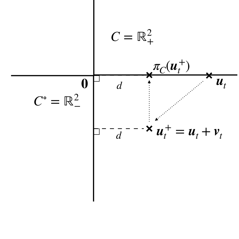
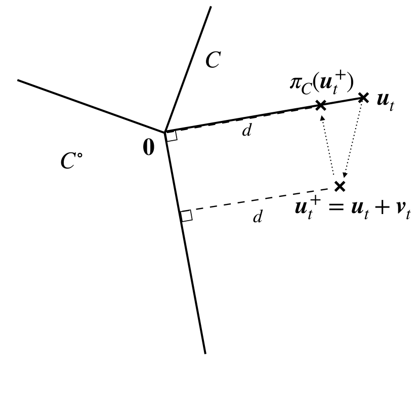
Let us give some intuition on the effect of projection onto 𝒞𝒞\mathcal{C}. In a geometric sense, it is easier to visualize things in 2superscript2\mathbb{R}^{2} with 𝒞=+2𝒞subscriptsuperscript2\mathcal{C}=\mathbb{R}^{2}_{+} and 𝒞=2superscript𝒞subscriptsuperscript2\mathcal{C}^{\circ}=\mathbb{R}^{2}_{-}. The projection on 𝒞𝒞\mathcal{C} moves the vector along the edges of 𝒞superscript𝒞\mathcal{C}^{\circ}, maintaining the distance to 𝒞superscript𝒞\mathcal{C}^{\circ} and moving toward the vector 𝟎0\bm{0}. This is illustrated in Figure 5 in Appendix B.1. From a game-theoretic standpoint, the projection on 𝒞=+2𝒞subscriptsuperscript2\mathcal{C}=\mathbb{R}^{2}_{+} eliminates the components of the payoffs that are negative. It enables CBA+ to be less pessimistic than CBA, which may accumulate negative payoffs on actions for a long time and never resets the components of the aggregated payoff to 00, leading to some actions being chosen less frequently.

We will see in the next section that RM+ is related to CBA+ but replaces the exact projection step π𝒞(𝒖)subscript𝜋𝒞𝒖\pi_{\mathcal{C}}(\bm{u}) in 𝖴𝖯𝖣𝖠𝖳𝖤𝖯𝖠𝖸𝖮𝖥𝖥𝖢𝖡𝖠+subscript𝖴𝖯𝖣𝖠𝖳𝖤𝖯𝖠𝖸𝖮𝖥𝖥𝖢𝖡𝖠+{\sf UPDATEPAYOFF}_{{\sf CBA\textsuperscript{+}}} by a suboptimal solution to the projection problem. Let us also note the difference between CBA+ and the algorithm introduced in Abernethy et al. (2011), which we have called CBA. CBA uses different UPDATEPAYOFF and CHOOSEDECISION functions. In CBA the payoff update is defined as

𝖴𝖯𝖣𝖠𝖳𝖤𝖯𝖠𝖸𝖮𝖥𝖥𝖢𝖡𝖠(𝒖,𝒙,𝒇,ω,S)=SS+ω𝒖+ωS+ω(𝒇/κ,𝒙,𝒇).subscript𝖴𝖯𝖣𝖠𝖳𝖤𝖯𝖠𝖸𝖮𝖥𝖥𝖢𝖡𝖠𝒖𝒙𝒇𝜔𝑆𝑆𝑆𝜔𝒖𝜔𝑆𝜔𝒇𝜅𝒙𝒇{\sf UPDATEPAYOFF}_{{\sf CBA}}(\bm{u},\bm{x},\bm{f},\omega,S)=\frac{S}{S+\omega}\bm{u}+\frac{\omega}{S+\omega}\left(\langle\bm{f}/\kappa,\bm{x}\rangle,-\bm{f}\right).

Note in particular the lack of projection as compared to CBA+, analogous to the difference between RM and RM+. The 𝖢𝖧𝖮𝖮𝖲𝖤𝖣𝖤𝖢𝖨𝖲𝖨𝖮𝖭𝖢𝖡𝖠subscript𝖢𝖧𝖮𝖮𝖲𝖤𝖣𝖤𝖢𝖨𝖲𝖨𝖮𝖭𝖢𝖡𝖠{\sf CHOOSEDECISION}_{{\sf CBA}} function then requires a projection onto 𝒞𝒞\mathcal{C}:

𝖢𝖧𝖮𝖮𝖲𝖤𝖣𝖤𝖢𝖨𝖲𝖨𝖮𝖭𝖢𝖡𝖠(𝒖)=𝖢𝖧𝖮𝖮𝖲𝖤𝖣𝖤𝖢𝖨𝖲𝖨𝖮𝖭𝖢𝖡𝖠+(π𝒞(𝒖)).subscript𝖢𝖧𝖮𝖮𝖲𝖤𝖣𝖤𝖢𝖨𝖲𝖨𝖮𝖭𝖢𝖡𝖠𝒖subscript𝖢𝖧𝖮𝖮𝖲𝖤𝖣𝖤𝖢𝖨𝖲𝖨𝖮𝖭𝖢𝖡𝖠+subscript𝜋𝒞𝒖{\sf CHOOSEDECISION}_{{\sf CBA}}(\bm{u})={\sf CHOOSEDECISION}_{{\sf CBA\textsuperscript{+}}}\left(\pi_{\mathcal{C}}(\bm{u})\right).

Based upon the analysis in Blackwell (1956), Abernethy et al. (2011) show that CBA with uniform weights (both on payoffs and decisions) guarantees O(1/T)𝑂1𝑇O(1/\sqrt{T}) average regret. The difference between CBA+ and CBA is similar to the difference between the RM and RM+ algorithms. In practice, RM+ performs significantly better than RM for solving matrix games, when combined with linear averaging on the decisions (as opposed to the uniform averaging used in Theorem 2.1). In the next theorem, we show that CBA+ is compatible with linear averaging on decisions only. We present a detailed proof in Appendix B.

Theorem 3.1.

Consider (𝐱t)t0subscriptsubscript𝐱𝑡𝑡0\left(\bm{x}_{t}\right)_{t\geq 0} generated by CBA+ with uniform weights: ωτ=1,τ1formulae-sequencesubscript𝜔𝜏1for-all𝜏1\omega_{\tau}=1,\forall\;\tau\geq 1. Let L=max{𝐟t2|t1}𝐿conditionalsubscriptnormsubscript𝐟𝑡2𝑡1L=\max\{\|\bm{f}_{t}\|_{2}\;|\;t\geq 1\} and κ=max{𝐱2|𝐱𝒳}𝜅conditionalsubscriptnorm𝐱2𝐱𝒳\kappa=\max\{\|\bm{x}\|_{2}\;|\;\bm{x}\in\mathcal{X}\}. Then

t=1Tt𝒇t,𝒙tmin𝒙𝒳t=1Tt𝒇t,𝒙T(T+1)=O(κL/T).superscriptsubscript𝑡1𝑇𝑡subscript𝒇𝑡subscript𝒙𝑡subscript𝒙𝒳superscriptsubscript𝑡1𝑇𝑡subscript𝒇𝑡𝒙𝑇𝑇1𝑂𝜅𝐿𝑇\dfrac{\sum_{t=1}^{T}t\langle\bm{f}_{t},\bm{x}_{t}\rangle-\min_{\bm{x}\in\mathcal{X}}\sum_{t=1}^{T}t\langle\bm{f}_{t},\bm{x}\rangle}{T(T+1)}=O\left(\kappa L/\sqrt{T}\right).

Note that in Theorem 3.1, we have uniform weights on the sequence of payoffs (𝒖t)t0subscriptsubscript𝒖𝑡𝑡0\left(\bm{u}_{t}\right)_{t\geq 0}, but linearly increasing weights on the sequence of decisions. The proof relies on properties specific to CBA+, and it does not extend to CBA. Numerically it also helps CBA+ but not CBA. In Appendix B, we show that both CBA and CBA+ achieve O(κL/T)𝑂𝜅𝐿𝑇O\left(\kappa L/\sqrt{T}\right) convergence rates when using a weighted average on both the decisions and the payoffs (Theorems B.2-B.3). In practice, using linear averaging only on the decisions, as in Theorem 3.1, performs vastly better than linear averaging on both decisions and payoffs. We present empirical evidence of this in Appendix B.

We can compare the O(κL/T)𝑂𝜅𝐿𝑇O\left(\kappa L/\sqrt{T}\right) average regret for CBA+ with the O(ΩL/T)𝑂Ω𝐿𝑇O\left(\Omega L/\sqrt{T}\right) average regret for OMD (Nemirovski and Yudin, 1983; Ben-Tal and Nemirovski, 2001) and FTRL (Abernethy et al., 2009; McMahan, 2011), where Ω=max{𝒙𝒙2|𝒙,𝒙𝒳}.Ωconditionalsubscriptnorm𝒙superscript𝒙2𝒙superscript𝒙𝒳\Omega=\max\{\|\bm{x}-\bm{x}^{\prime}\|_{2}|\bm{x},\bm{x}^{\prime}\in\mathcal{X}\}. We can always recenter 𝒳𝒳\mathcal{X} to contain 𝟎0\bm{0}, in which case the bounds for OMD/FTRL and CBA+ are equivalent since κΩ2κ𝜅Ω2𝜅\kappa\leq\Omega\leq 2\kappa. Note that the bound on the average regret for Optimistic OMD (O-OMD, Chiang et al. (2012)) and Optimistic FTRL (O-FTRL, Rakhlin and Sridharan (2013)) is O(Ω2L/T)𝑂superscriptΩ2𝐿𝑇O\left(\Omega^{2}L/T\right) in the game setup, a priori better than the bound for CBA+ as regards the number of iterations T𝑇T. Nonetheless, we will see in Section 4 that the empirical performance of CBA+ is better than that of O(1/T)𝑂1𝑇O(1/T) methods. A similar situation occurs for RM+ compared to O-OMD and O-FTRL for solving poker games (Farina et al., 2019b; Kroer et al., 2020).

The following theorem gives the convergence rate of CBA+ for solving saddle-points (1), based on our convergence rate on the regret of each player (Theorem 3.1). The proof is in Appendix C.

Theorem 3.2.

Let (𝐱¯T,𝐲¯T)=2t=1Tt(𝐱t,𝐲t)/(T(T+1)),subscript¯𝐱𝑇subscript¯𝐲𝑇2superscriptsubscript𝑡1𝑇𝑡subscript𝐱𝑡subscript𝐲𝑡𝑇𝑇1\left(\bar{\bm{x}}_{T},\bar{\bm{y}}_{T}\right)=2\sum_{t=1}^{T}t\left(\bm{x}_{t},\bm{y}_{t}\right)/(T(T+1)), where (𝐱t)t0,(𝐲t)t0subscriptsubscript𝐱𝑡𝑡0subscriptsubscript𝐲𝑡𝑡0\left(\bm{x}_{t}\right)_{t\geq 0},\left(\bm{y}_{t}\right)_{t\geq 0} are generated by the repeated game framework with CBA+ with uniform weights: ωτ=1,τ1formulae-sequencesubscript𝜔𝜏1for-all𝜏1\omega_{\tau}=1,\forall\;\tau\geq 1. Let L=max{Lx,Ly}𝐿subscript𝐿𝑥subscript𝐿𝑦L=\max\{L_{x},L_{y}\} defined in (3) and κ=max{max{𝐱2,𝐲2}|𝐱𝒳,𝐲𝒴}𝜅conditionalsubscriptnorm𝐱2subscriptnorm𝐲2𝐱𝒳𝐲𝒴\kappa=\max\{\max\{\|\bm{x}\|_{2},\|\bm{y}\|_{2}\}\;|\;\bm{x}\in\mathcal{X},\bm{y}\in\mathcal{Y}\}. Then

max𝒚𝒴F(𝒙¯T,𝒚)min𝒙𝒳F(𝒙,𝒚¯T)=O(κL/T).subscript𝒚𝒴𝐹subscript¯𝒙𝑇𝒚subscript𝒙𝒳𝐹𝒙subscript¯𝒚𝑇𝑂𝜅𝐿𝑇\max_{\bm{y}\in\mathcal{Y}}F(\bar{\bm{x}}_{T},\bm{y})-\min_{\bm{x}\in\mathcal{X}}F(\bm{x},\bar{\bm{y}}_{T})=O\left(\kappa L/\sqrt{T}\right).

3.1 Efficient implementations of CBA+

To obtain an implementation of CBA+ and CBA, we need to efficiently resolve the functions 𝖢𝖧𝖮𝖮𝖲𝖤𝖣𝖤𝖢𝖨𝖲𝖨𝖮𝖭𝖢𝖡𝖠+subscript𝖢𝖧𝖮𝖮𝖲𝖤𝖣𝖤𝖢𝖨𝖲𝖨𝖮𝖭𝖢𝖡𝖠+{\sf CHOOSEDECISION}_{{\sf CBA\textsuperscript{+}}}{} and 𝖴𝖯𝖣𝖠𝖳𝖤𝖯𝖠𝖸𝖮𝖥𝖥𝖢𝖡𝖠+subscript𝖴𝖯𝖣𝖠𝖳𝖤𝖯𝖠𝖸𝖮𝖥𝖥𝖢𝖡𝖠+{\sf UPDATEPAYOFF}_{{\sf CBA\textsuperscript{+}}{}}. In particular, we need to compute π𝒞(𝒖)subscript𝜋𝒞𝒖\pi_{\mathcal{C}}(\bm{u}), the orthogonal projection of 𝒖𝒖\bm{u} onto the cone 𝒞𝒞\mathcal{C}, where 𝒞=cone({κ}×𝒳)𝒞cone𝜅𝒳\mathcal{C}=\textrm{cone}(\{\kappa\}\times\mathcal{X}):

π𝒞(𝒖)argmin𝒚𝒞𝒚𝒖22.subscript𝜋𝒞𝒖subscript𝒚𝒞superscriptsubscriptnorm𝒚𝒖22\pi_{\mathcal{C}}(\bm{u})\in\arg\min_{\bm{y}\in\mathcal{C}}\|\bm{y}-\bm{u}\|_{2}^{2}. (4)

Even for CBA this problem must be resolved, since Abernethy et al. (2011) did not study whether (4) can be efficiently solved. It turns out that (4) can be computed in closed-form or quasi closed-form for many decision sets 𝒳𝒳\mathcal{X} of interest. Interestingly, parts of the proofs rely on Moreau’s Decomposition Theorem (Combettes and Reyes, 2013), which states that π𝒞(𝒖)subscript𝜋𝒞𝒖\pi_{\mathcal{C}}(\bm{u}) can be recovered from π𝒞(𝒖)subscript𝜋superscript𝒞𝒖\pi_{\mathcal{C}^{\circ}}(\bm{u}) and vice-versa, because π𝒞(𝒖)+π𝒞(𝒖)=𝒖.subscript𝜋𝒞𝒖subscript𝜋superscript𝒞𝒖𝒖\pi_{\mathcal{C}}(\bm{u})+\pi_{\mathcal{C}^{\circ}}(\bm{u})=\bm{u}. We present the detailed complexity results and the proofs in Appendix D.

Simplex

𝒳=Δ(n)𝒳Δ𝑛\mathcal{X}=\Delta(n) is the classical setting used for matrix games. Also, for extensive-form games, CFR decomposes the decision sets (treeplexes) into a set of regret minimization problems over the simplex (Farina et al., 2019a). Here, n𝑛n is the number of actions of a player and 𝒙Δ(n)𝒙Δ𝑛\bm{x}\in\Delta(n) represents a randomized strategy. In this case, π𝒞(𝒖)subscript𝜋𝒞𝒖\pi_{\mathcal{C}}(\bm{u}) can be computed in O(nlog(n))𝑂𝑛𝑛O(n\log(n)). Note that RM and RM+ are obtained by choosing a suboptimal solution to (4), avoiding the O(nlog(n))𝑂𝑛𝑛O(n\log(n)) sorting operation, whereas CBA and CBA+ choose optimally (see Appendix D). Thus, RM and RM+ can be seen as approximate versions of CBA and CBA+, where (4) is solved approximatively at every iteration. In our numerical experiments, we will see that CBA+ slightly outperforms RM+ and CFR+ in terms of iteration count.

psubscript𝑝\ell_{p} balls

This is when 𝒳={𝒙n|;𝒙p1}\mathcal{X}=\{\bm{x}\in\mathbb{R}^{n}\;|\ ;\|\bm{x}\|_{p}\leq 1\} with p1𝑝1p\geq 1 or p=𝑝p=\infty. This is of interest for instance in distributionally robust optimization (Ben-Tal et al., 2015; Namkoong and Duchi, 2016), subscript\ell_{\infty} regression (Sidford and Tian, 2018) and saddle-point reformulation of Markov Decision Process (Jin and Sidford, 2020). For p=2𝑝2p=2, we can compute π𝒞(𝒖)subscript𝜋𝒞𝒖\pi_{\mathcal{C}}(\bm{u}) in closed-form, i.e., in O(n)𝑂𝑛O(n) arithmetic operations. For p{1,}𝑝1p\in\{1,\infty\}, we can compute π𝒞(𝒖)subscript𝜋𝒞𝒖\pi_{\mathcal{C}}(\bm{u}) in O(nlog(n))𝑂𝑛𝑛O(n\log(n)) arithmetic operations using a sorting algorithm.

Ellipsoidal confidence region in the simplex

Here, 𝒳𝒳\mathcal{X} is an ellipsoidal subregion of the simplex, defined as 𝒳={𝒙Δ(n)|𝒙𝒙02ϵx}𝒳conditional-set𝒙Δ𝑛subscriptnorm𝒙subscript𝒙02subscriptitalic-ϵ𝑥\mathcal{X}=\{\bm{x}\in\Delta(n)\;|\;\|\bm{x}-\bm{x}_{0}\|_{2}\leq\epsilon_{x}\}. This type of decision set is widely used because it is associated with confidence regions when estimating a probability distribution from observed data (Iyengar, 2005; Bertsimas et al., 2019). It can also be used in the Bellman update for robust Markov Decision Process (Iyengar, 2005; Wiesemann et al., 2013; Goyal and Grand-Clément, 2018). We also assume that the confidence region is “entirely contained in the simplex”: {𝒙n|𝒙𝒆=1}{𝒙n|𝒙𝒙02ϵx}Δ(n)conditional-set𝒙superscript𝑛superscript𝒙top𝒆1conditional-set𝒙superscript𝑛subscriptnorm𝒙subscript𝒙02subscriptitalic-ϵ𝑥Δ𝑛\{\bm{x}\in\mathbb{R}^{n}|\bm{x}^{\top}\bm{e}=1\}\bigcap\{\bm{x}\in\mathbb{R}^{n}\;|\;\|\bm{x}-\bm{x}_{0}\|_{2}\leq\epsilon_{x}\}\subseteq\Delta(n), to avoid degenerate components. In this case, using a change of basis we show that it is possible to compute π𝒞(𝒖)subscript𝜋𝒞𝒖\pi_{\mathcal{C}}(\bm{u}) in closed-form, i.e., in O(n)𝑂𝑛O(n) arithmetic operations.

Other potential sets of interests

Other important decision sets include sets based on Kullback-Leibler divergence {𝒙Δ(n)|KL(𝒙,𝒙0)ϵx}conditional-set𝒙Δ𝑛𝐾𝐿𝒙subscript𝒙0subscriptitalic-ϵ𝑥\{\bm{x}\in\Delta(n)\;|\;KL\left(\bm{x},\bm{x}_{0}\right)\leq\epsilon_{x}\}, or, more generally, ϕitalic-ϕ\phi-divergence (Ben-Tal et al., 2013). For these sets, we did not find a closed-form solution to the projection problem (4). Still, as long as the domain 𝒳𝒳\mathcal{X} is a convex set, computing π𝒞(𝒖)subscript𝜋𝒞𝒖\pi_{\mathcal{C}}(\bm{u}) remains a convex problem, and it can be solved efficiently with solvers, although this results in a slower algorithm than with closed-form computations of π𝒞(𝒖)subscript𝜋𝒞𝒖\pi_{\mathcal{C}}(\bm{u}).

4 Numerical experiments

In this section we investigate the practical performances of our algorithms on several instances of saddle-point problems. We start by comparing CBA+ with RM+ in the matrix and extensive-form games setting. We then turn to comparing our algorithms on instances from the distributionally robust optimization literature. The code for all experiments is available in the supplemental material.

4.1 Matrix games on the simplex and Extensive-Form Games

Since the motivation for CBA+ is to obtain the strong empirical performances of RM+ and CFR+ on other decision sets than the simplex, we start by checking that CBA+ indeed provide comparable performance on simplex settings. We compare these methods on matrix games

min𝒙Δ(n)max𝒚Δ(m)𝒙,𝑨𝒚,subscript𝒙Δ𝑛subscript𝒚Δ𝑚𝒙𝑨𝒚\min_{\bm{x}\in\Delta(n)}\max_{\bm{y}\in\Delta(m)}\langle\bm{x},\bm{Ay}\rangle,

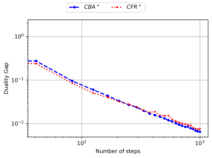
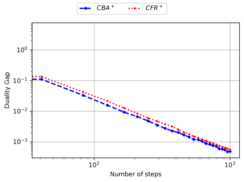
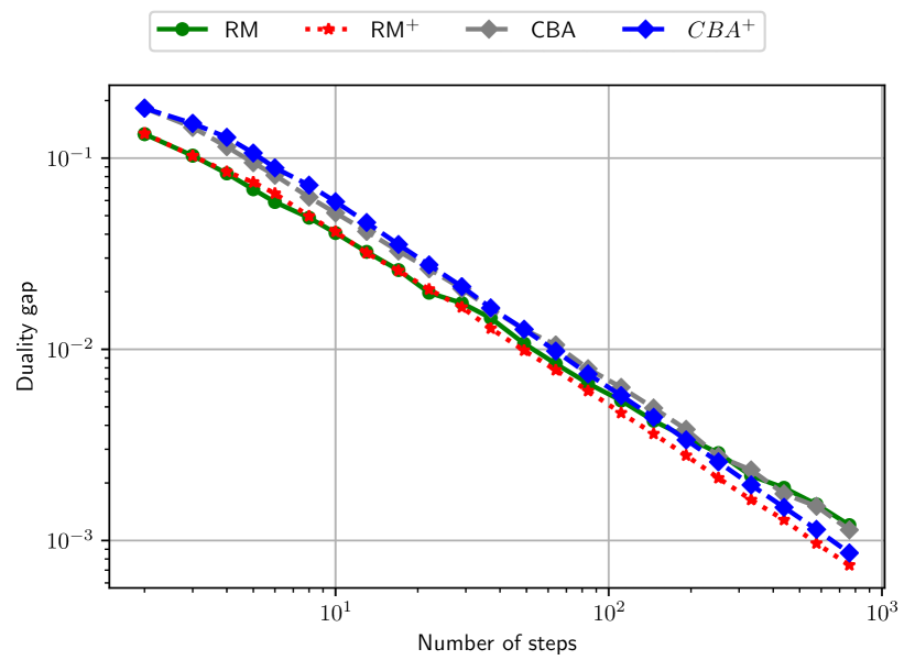
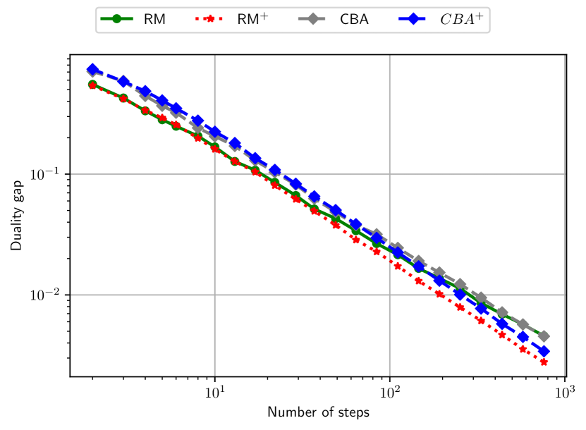
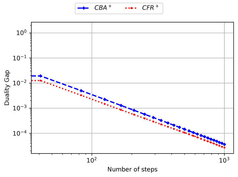
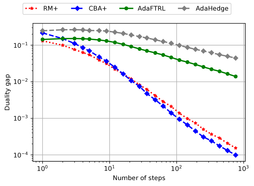
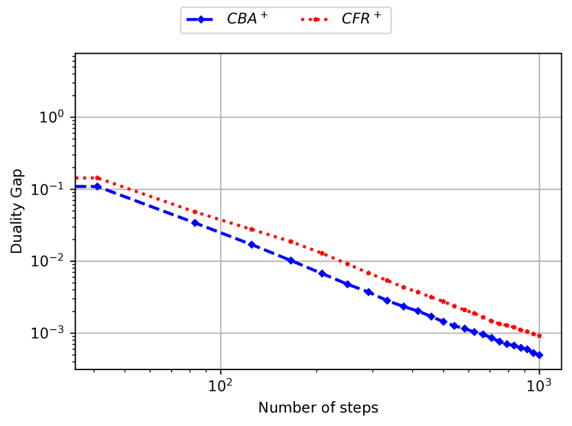
where 𝑨𝑨\bm{A} is the matrix of payoff, and on extensive-form games (EFGs). EFGs can also be written as SPPs with bilinear objective and 𝒳,𝒴𝒳𝒴\mathcal{X},\mathcal{Y} polytopes encoding the players’ space of sequential strategies (von Stengel, 1996). EFGs can be solved via simplex-based regret minimization by using the counterfactual regret minimization (CFR) framework to decompose regrets into local regrets at each simplex. Explaining CFR is beyond the scope of this work; we point the reader to (Zinkevich et al., 2007) or newer explanations (Farina et al., 2019c, a). For matrix games, we generate 70 synthetic 101010-dimensional matrix games with AijU[0,1]similar-tosubscript𝐴𝑖𝑗𝑈01A_{ij}\sim U[0,1] and compare the most efficient algorithms for matrix games with linear averaging: CBA+ and RM+. We also compare with two other scale-free no-regret algorithms, AdaHedge (De Rooij et al., 2014) and AdaFTRL (Orabona and Pál, 2015). Figure 1(a) presents the duality gap of the current solutions vs. the number of steps. Here, both CBA+ and RM+ use alternation, which is a trick that is well-known to improve the performances of RM+ (Tammelin et al., 2015), where the repeated game framework is changed such that players take turns updating their strategies, rather than performing these updates simultaneously, see Appendix E.1 for details.111We note that RM+ is guaranteed to retain its convergence rate under alternation. In contrast, we leave resolving this property for CBA+ to future work.

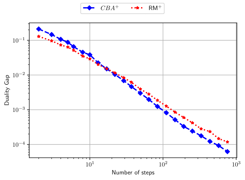
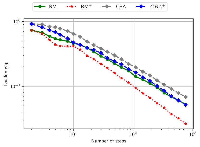
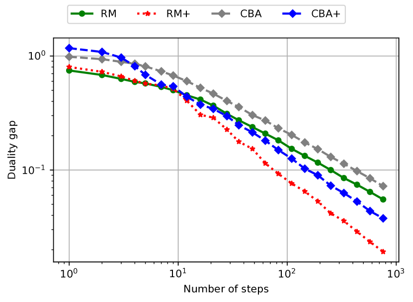
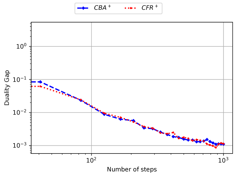
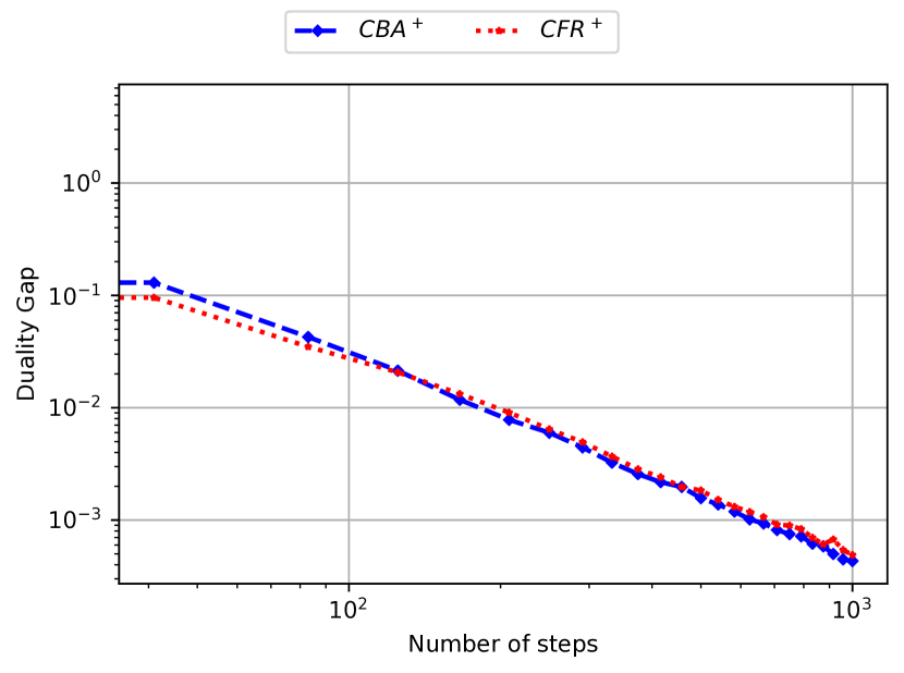
For EFGs, we compare CBA+and CFR+ on many poker AI benchmark instances, including Leduc, Kuhn, search games and sheriff (see Farina et al. (2021) for game descriptions). We present our results in Figures 1(b)-1(d). Additional details and experiments for EFGs are presented in Appendix E.4. Overall, we see in Figure 1 that CBA+may slightly outperform RM+ and CFR+, two of the strongest algorithms for matrix games and EFGs, which were shown to achieve the best empirical performances compared to a wide range of algorithms, including Hedge and other first-order methods (Kroer, 2020; Kroer et al., 2018; Farina et al., 2019b). For matrix games, AdaHedge and AdaFTRL are both outperformed by RM+ and CBA+; we present more experiments to compare RM+ and CBA+ in Appendix E.2, and more experiments with matrix games in Appendix E.3. Recall that our goal is to generalize these strong performance to other settings: we present our numerical experiments for solving distributionally robust optimization problems in the next section.
Refer to caption
(a) Matrix game.
Refer to caption
(b) EFG: Leduc, 2 players, 9 ranks.
Refer to caption
(c) EFG: Battleship, 3 turns, 1 ship.
Refer to caption
(d) EFG: Leduc, 2 players, 5 ranks.
Figure 1: Comparison of CBA+ with RM+ and CFR+ on matrix games and EFGs.

4.2 Distributionally Robust Optimization

Problem setup

Broadly speaking, DRO attempts to exploit partial knowledge of the statistical properties of the model parameters to obtain risk-averse optimal solutions (Rahimian and Mehrotra, 2019). We focus on the following instance of distributionally robust classification with logistic losses (Namkoong and Duchi, 2016; Ben-Tal et al., 2015). There are m𝑚m observed feature-label pairs (𝒂i,bi)n×{1,1}subscript𝒂𝑖subscript𝑏𝑖superscript𝑛11\left(\bm{a}_{i},b_{i}\right)\in\mathbb{R}^{n}\times\{-1,1\}, and we want to solve

min𝒙n,𝒙𝒙02Rmax𝒚Δ(m),𝒚𝒚022λi=1myii(𝒙),subscriptformulae-sequence𝒙superscript𝑛subscriptnorm𝒙subscript𝒙02𝑅subscriptformulae-sequence𝒚Δ𝑚superscriptsubscriptnorm𝒚subscript𝒚022𝜆superscriptsubscript𝑖1𝑚subscript𝑦𝑖subscript𝑖𝒙\min_{\bm{x}\in\mathbb{R}^{n},\|\bm{x}-\bm{x}_{0}\|_{2}\leq R}\max_{\bm{y}\in\Delta(m),\|\bm{y}-\bm{y}_{0}\|_{2}^{2}\leq\lambda}\sum_{i=1}^{m}y_{i}\ell_{i}(\bm{x}), (5)

where i(𝒙)=log(1+exp(bi𝒂i𝒙))subscript𝑖𝒙1subscript𝑏𝑖subscriptsuperscript𝒂top𝑖𝒙\ell_{i}(\bm{x})=\log(1+\exp(-b_{i}\bm{a}^{\top}_{i}\bm{x})). The formulation (5) takes a worst-case approach to put more weight on misclassified observations and provides some statistical guarantees, e.g., it can be seen as a convex regularization of standard empirical risk minimization instances (Duchi et al., 2021).

We compare CBA+ (with linear averaging and alternation) with Online Mirror Descent (OMD), Optimistic OMD (O-OMD), Follow-The-Regularized-Leader (FTRL) and Optimistic FTRL (O-FTRL). We provide a detailed presentation of our implementations of these algorithms in Appendix F. We compare the performances of these algorithms with CBA+ on two synthetic data sets and four real data sets. We use linear averaging on decisions for all algorithms, and parameters 𝒙0=𝟎,R=10,𝒚0=(1,,1)/m,λ=1/2mformulae-sequencesubscript𝒙00formulae-sequence𝑅10formulae-sequencesubscript𝒚011𝑚𝜆12𝑚\bm{x}_{0}=\bm{0},R=10,\bm{y}_{0}=\left(1,...,1\right)/m,\lambda=1/2m in eq. 5.

Synthetic and real instances

For the synthetic classification instances, we generate an optimal 𝒙nsuperscript𝒙superscript𝑛\bm{x}^{*}\in\mathbb{R}^{n}, sample 𝒂iN(0,𝑰)similar-tosubscript𝒂𝑖𝑁0𝑰\bm{a}_{i}\sim N(0,\bm{I}) for i{1,,m}𝑖1𝑚i\in\{1,...,m\}, set labels bi=sign(𝒂i𝒙)subscript𝑏𝑖signsubscriptsuperscript𝒂top𝑖superscript𝒙b_{i}=\text{sign}(\bm{a}^{\top}_{i}\bm{x}^{*}), and then we flip 10%percent1010\% of them. For the real classification instances, we use the following data sets from the libsvm website222https://www.csie.ntu.edu.tw/similar-to\simcjlin/libsvmtools/datasets/: adult, australian, splice, madelon. Details about the empirical setting, the data sets and additional numerical experiments are presented in Appendix G.

Choice of step sizes

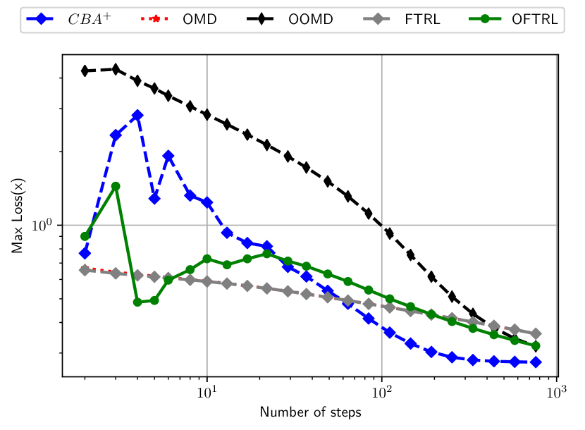
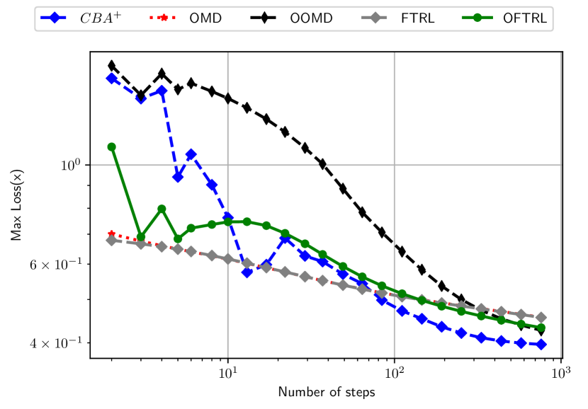
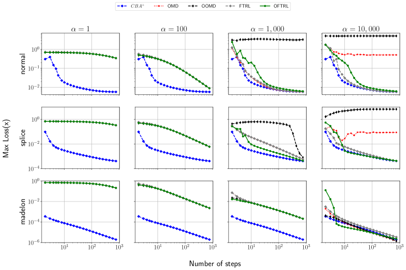
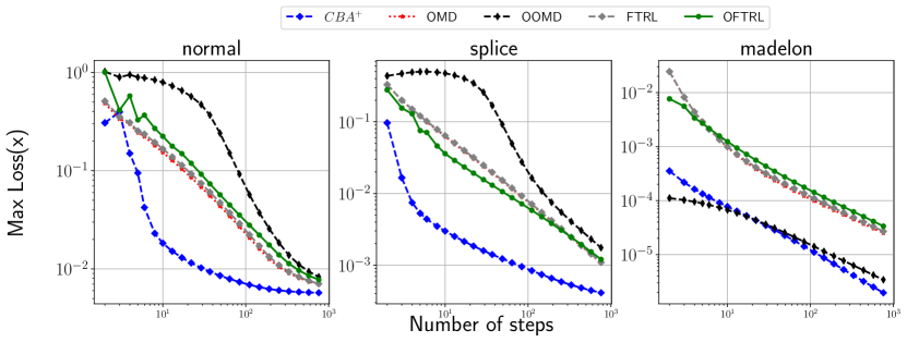
One of the main motivation for CBA+ is to obtain a parameter-free algorithm. Choosing a fixed step size η𝜂\eta for the other algorithms requires knowing a bound L𝐿L on the norm of the instantaneous payoffs (see Appendix F.2 for our derivations of this upper bound). This is a major limitation in practice: these bounds may be very conservative, leading to small step sizes. We highlight this by showing the performance of all four algorithms, for various fixed step sizes η=α×η𝗍𝗁𝜂𝛼subscript𝜂𝗍𝗁\eta=\alpha\times\eta_{\sf th}, where α{1,100,1,000,10,000}𝛼1100100010000\alpha\in\{1,100,1,000,10,000\} is a multiplier and η𝗍𝗁subscript𝜂𝗍𝗁\eta_{\sf th} is the theoretical step size which guarantees the convergence of the algorithms for each instance. We detail the computation of η𝗍𝗁subscript𝜂𝗍𝗁\eta_{\sf th} in Appendix F.2. We present the results of our numerical experiments on synthetic and real data sets in Figure 2. Additional simulations with adaptive step sizes ηt=1/τ=1t1𝒇τ22subscript𝜂𝑡1superscriptsubscript𝜏1𝑡1superscriptsubscriptnormsubscript𝒇𝜏22\eta_{t}=1/\sqrt{\sum_{\tau=1}^{t-1}\|\bm{f}_{\tau}\|_{2}^{2}} (Orabona, 2019) are presented in Figure 3 and in Appendix G.
Refer to caption
Figure 2: Comparisons of the performances of CBA+ with OMD,FTRL,O-OMD and O-FTRL with fixed step sizes, on synthetic (with normal distribution) and real data sets (splice and madelon).

Results and discussion

In Figure 2, we present the worst-case loss of the current solution 𝒙¯Tsubscript¯𝒙𝑇\bar{\bm{x}}_{T} in terms of the number of steps T𝑇T. We see that when the step sizes is chosen as the theoretical step sizes guaranteeing the convergence of the non-parameter free algorithms (α=1𝛼1\alpha=1), CBA+ vastly outperforms all of the algorithms. When we take more aggressive step sizes, the non-parameter-free algorithms become more competitive. For instance, when α=1,000𝛼1000\alpha=1,000, OMD, FTRL and O-FTRL are competitive with CBA+ for the experiments on synthetic data sets. However, for this same instance and α=1,000𝛼1000\alpha=1,000, O-OMD diverges, because the step sizes are far greater than the theoretical step sizes guaranteeing convergence. At α=10,000𝛼10000\alpha=10,000, both OMD and O-OMD diverge. The same type of performances also hold for the splice data set. Finally, for the madelon data set, the non parameter-free algorithms start to be competitive with CBA+ only when α=10,000𝛼10000\alpha=10,000. Again, we note that this range of step sizes η𝜂\eta is completely outside the values η𝗍𝗁subscript𝜂𝗍𝗁\eta_{\sf th} that guarantee convergence of the algorithms, and fine-tuning the algorithms is time- and resource-consuming. In contrast, CBA+ can be used without wasting time on exploring and finding the best convergence rates, and with confidence in the convergence of the algorithm. Similar observations hold for adaptive step sizes (see Figure 3 and Appendix G). The overall poor performances of the optimistic methods (compared to their O(1/T)𝑂1𝑇O(1/T) average regret guarantees) may reflect their sensibility to the choice of the step sizes. Additional experiments in Appendix G with other real and synthetic EFG and DRO instances show the robustness of the strong performances of CBA+ across additional problem instances.
Refer to caption
Figure 3: Comparisons of the performances of CBA+, OMD,FTRL,O-OMD and O-FTRL with adaptive step sizes, on synthetic (with normal distribution) and real data sets (splice and madelon).

Running times compared to CBA+

We would like to emphasize that all of our figures show the number of steps on the x𝑥x-axis, and not the actual running times of the algorithms. Overall, CBA+ converges to an optimal solution to the DRO instance (5) vastly faster than the other algorithms. In particular, empirically, CBA+ is 2x-2.5x faster than OMD, FTRL and O-FTRL, and 3x-4x faster than O-OMD. This is because OMD, FTRL, O-OMD, and O-FTRL require binary searches at each step, see Appendix F. The functions used in the binary searches themselves require solving an optimization program (an orthogonal projection onto the simplex, see (33)) at each evaluation. Even though computing the orthogonal projection of a vector onto the simplex can be done in O(nlog(n))𝑂𝑛𝑛O(n\log(n)), this results in slower overall running time, compared to CBA+ with (quasi) closed-form updates at each step. The situation is even worse for O-OMD, which requires two proximal updates at each iteration. We acknowledge that the same holds for CBA+ compared to RM+. In particular, CBA+ is slightly slower than RM+, because of the computation of π𝒞(𝒖)subscript𝜋𝒞𝒖\pi_{\mathcal{C}}(\bm{u}) in O(nlog(n))𝑂𝑛𝑛O(n\log(n)) operations at every iteration.

5 Conclusion

We have introduced CBA+, a new algorithm for convex-concave saddle-point solving, that is 1) simple to implement for many practical decision sets, 2) completely parameter-free and does not attempt to lear any step sizes, and 3) competitive with, or even better than, state-of-the-art approaches for the best choices of parameters, both for matrix games, extensive-form games, and distributionally robust instances. Our paper is based on Blackwell approachability, which has been used to achieved important breakthroughs in poker AI in recent years, and we hope to generalize the use and implementation of this framework to other important problem instances. Interesting future directions of research include developing a theoretical understanding of the improvements related to alternation in our setting, designing efficient implementations for other widespread decision sets (e.g., based on Kullback-Leibler divergence or ϕitalic-ϕ\phi-divergence), and novel accelerated versions based on strong convex-concavity or optimistim.

Societal impact

Our work enables faster and simpler computation of solutions of saddle-point problems, which have become widely used for applications in the industry. There is a priori no direct negative societal consequence to this work, since our methods simply return the same solutions as previous algorithms but in a simpler and more efficient way.

References

  • Abernethy et al. [2011] Jacob Abernethy, Peter L Bartlett, and Elad Hazan. Blackwell approachability and no-regret learning are equivalent. In Proceedings of the 24th Annual Conference on Learning Theory, pages 27–46. JMLR Workshop and Conference Proceedings, 2011.
  • Abernethy et al. [2009] Jacob D Abernethy, Elad Hazan, and Alexander Rakhlin. Competing in the dark: An efficient algorithm for bandit linear optimization. 2009.
  • Beck and Teboulle [2003] Amir Beck and Marc Teboulle. Mirror descent and nonlinear projected subgradient methods for convex optimization. Operations Research Letters, 31(3):167–175, 2003.
  • Ben-Tal and Nemirovski [2001] Aharon Ben-Tal and Arkadi Nemirovski. Lectures on modern convex optimization: analysis, algorithms, and engineering applications, volume 2. Siam, 2001.
  • Ben-Tal et al. [2013] Aharon Ben-Tal, Dick Den Hertog, Anja De Waegenaere, Bertrand Melenberg, and Gijs Rennen. Robust solutions of optimization problems affected by uncertain probabilities. Management Science, 59(2):341–357, 2013.
  • Ben-Tal et al. [2015] Aharon Ben-Tal, Elad Hazan, Tomer Koren, and Shie Mannor. Oracle-based robust optimization via online learning. Operations Research, 63(3):628–638, 2015.
  • Bertsimas et al. [2019] Dimitris Bertsimas, Dick den Hertog, and Jean Pauphilet. Probabilistic guarantees in robust optimization. 2019.
  • Blackwell [1956] David Blackwell. An analog of the minimax theorem for vector payoffs. Pacific Journal of Mathematics, 6(1):1–8, 1956.
  • Bowling et al. [2015] Michael Bowling, Neil Burch, Michael Johanson, and Oskari Tammelin. Heads-up limit hold’em poker is solved. Science, 347(6218):145–149, 2015.
  • Brown and Sandholm [2018] Noam Brown and Tuomas Sandholm. Superhuman AI for heads-up no-limit poker: Libratus beats top professionals. Science, 359(6374):418–424, 2018.
  • Brown and Sandholm [2019] Noam Brown and Tuomas Sandholm. Superhuman AI for multiplayer poker. Science, 365(6456):885–890, 2019.
  • Burch et al. [2019] Neil Burch, Matej Moravcik, and Martin Schmid. Revisiting cfr+ and alternating updates. Journal of Artificial Intelligence Research, 64:429–443, 2019.
  • Chambolle and Pock [2011] Antonin Chambolle and Thomas Pock. A first-order primal-dual algorithm for convex problems with applications to imaging. Journal of mathematical imaging and vision, 40(1):120–145, 2011.
  • Chambolle and Pock [2016] Antonin Chambolle and Thomas Pock. On the ergodic convergence rates of a first-order primal–dual algorithm. Mathematical Programming, 159(1-2):253–287, 2016.
  • Chiang et al. [2012] Chao-Kai Chiang, Tianbao Yang, Chia-Jung Lee, Mehrdad Mahdavi, Chi-Jen Lu, Rong Jin, and Shenghuo Zhu. Online optimization with gradual variations. In Conference on Learning Theory, pages 6–1. JMLR Workshop and Conference Proceedings, 2012.
  • Combettes and Reyes [2013] Patrick L Combettes and Noli N Reyes. Moreau’s decomposition in banach spaces. Mathematical Programming, 139(1):103–114, 2013.
  • De Rooij et al. [2014] Steven De Rooij, Tim Van Erven, Peter D Grünwald, and Wouter M Koolen. Follow the leader if you can, hedge if you must. The Journal of Machine Learning Research, 15(1):1281–1316, 2014.
  • Duchi et al. [2008] John Duchi, Shai Shalev-Shwartz, Yoram Singer, and Tushar Chandra. Efficient projections onto the L-1 ball for learning in high dimensions. In Proceedings of the 25th international conference on Machine learning, pages 272–279, 2008.
  • Duchi et al. [2021] John C Duchi, Peter W Glynn, and Hongseok Namkoong. Statistics of robust optimization: A generalized empirical likelihood approach. Mathematics of Operations Research, 2021.
  • Egozcue et al. [2003] Juan José Egozcue, Vera Pawlowsky-Glahn, Glòria Mateu-Figueras, and Carles Barcelo-Vidal. Isometric logratio transformations for compositional data analysis. Mathematical Geology, 35(3):279–300, 2003.
  • Farina et al. [2019a] Gabriele Farina, Christian Kroer, and Tuomas Sandholm. Online convex optimization for sequential decision processes and extensive-form games. In Proceedings of the AAAI Conference on Artificial Intelligence, volume 33, pages 1917–1925, 2019a.
  • Farina et al. [2019b] Gabriele Farina, Christian Kroer, and Tuomas Sandholm. Optimistic regret minimization for extensive-form games via dilated distance-generating functions. In Advances in Neural Information Processing Systems, pages 5222–5232, 2019b.
  • Farina et al. [2019c] Gabriele Farina, Christian Kroer, and Tuomas Sandholm. Regret circuits: Composability of regret minimizers. In International Conference on Machine Learning, pages 1863–1872, 2019c.
  • Farina et al. [2021] Gabriele Farina, Christian Kroer, and Tuomas Sandholm. Faster game solving via predictive blackwell approachability: Connecting regret matching and mirror descent. In Proceedings of the AAAI Conference on Artificial Intelligence. AAAI, 2021.
  • Gao et al. [2019] Yuan Gao, Christian Kroer, and Donald Goldfarb. Increasing iterate averaging for solving saddle-point problems. arXiv preprint arXiv:1903.10646, 2019.
  • Gordon [2007] Geoffrey J Gordon. No-regret algorithms for online convex programs. In Advances in Neural Information Processing Systems, pages 489–496. Citeseer, 2007.
  • Goyal and Grand-Clément [2018] Vineet Goyal and Julien Grand-Clément. Robust Markov decision process: Beyond rectangularity. arXiv preprint arXiv:1811.00215, 2018.
  • Grand-Clément and Kroer [2020a] Julien Grand-Clément and Christian Kroer. First-order methods for Wasserstein distributionally robust MDP. arXiv preprint arXiv:2009.06790, 2020a.
  • Grand-Clément and Kroer [2020b] Julien Grand-Clément and Christian Kroer. Scalable first-order methods for robust mdps. arXiv preprint arXiv:2005.05434, 2020b.
  • Hart and Mas-Colell [2000] Sergiu Hart and Andreu Mas-Colell. A simple adaptive procedure leading to correlated equilibrium. Econometrica, 68(5):1127–1150, 2000.
  • Iyengar [2005] Garud Iyengar. Robust dynamic programming. Mathematics of Operations Research, 30(2):257–280, 2005.
  • Jin and Sidford [2020] Yujia Jin and Aaron Sidford. Efficiently solving mdps with stochastic mirror descent. In International Conference on Machine Learning, pages 4890–4900. PMLR, 2020.
  • Kroer [2020] Christian Kroer. Ieor8100: Economics, ai, and optimization lecture note 5: Computing Nash equilibrium via regret minimization. 2020.
  • Kroer et al. [2018] Christian Kroer, Gabriele Farina, and Tuomas Sandholm. Solving large sequential games with the excessive gap technique. In Advances in Neural Information Processing Systems, pages 864–874, 2018.
  • Kroer et al. [2020] Christian Kroer, Kevin Waugh, Fatma Kılınç-Karzan, and Tuomas Sandholm. Faster algorithms for extensive-form game solving via improved smoothing functions. Mathematical Programming, pages 1–33, 2020.
  • McMahan [2011] Brendan McMahan. Follow-the-regularized-leader and mirror descent: Equivalence theorems and l1 regularization. In Proceedings of the Fourteenth International Conference on Artificial Intelligence and Statistics, pages 525–533. JMLR Workshop and Conference Proceedings, 2011.
  • Moravčík et al. [2017] Matej Moravčík, Martin Schmid, Neil Burch, Viliam Lisỳ, Dustin Morrill, Nolan Bard, Trevor Davis, Kevin Waugh, Michael Johanson, and Michael Bowling. Deepstack: Expert-level artificial intelligence in heads-up no-limit poker. Science, 356(6337):508–513, 2017.
  • Namkoong and Duchi [2016] Hongseok Namkoong and John C Duchi. Stochastic gradient methods for distributionally robust optimization with f-divergences. In NIPS, volume 29, pages 2208–2216, 2016.
  • Nemirovski [2004] Arkadi Nemirovski. Prox-method with rate of convergence O(1/t) for variational inequalities with lipschitz continuous monotone operators and smooth convex-concave saddle point problems. SIAM Journal on Optimization, 15(1):229–251, 2004.
  • Nemirovski and Yudin [1983] Arkadi Nemirovski and David Yudin. Problem complexity and method efficiency in optimization. 1983.
  • Orabona [2019] Francesco Orabona. A modern introduction to online learning. arXiv preprint arXiv:1912.13213, 2019.
  • Orabona and Pál [2015] Francesco Orabona and Dávid Pál. Scale-free algorithms for online linear optimization. In International Conference on Algorithmic Learning Theory, pages 287–301. Springer, 2015.
  • Rahimian and Mehrotra [2019] Hamed Rahimian and Sanjay Mehrotra. Distributionally robust optimization: A review. arXiv preprint arXiv:1908.05659, 2019.
  • Rakhlin and Sridharan [2013] Alexander Rakhlin and Karthik Sridharan. Online learning with predictable sequences. In Conference on Learning Theory, pages 993–1019. PMLR, 2013.
  • Shimkin [2016] Nahum Shimkin. An online convex optimization approach to blackwell’s approachability. The Journal of Machine Learning Research, 17(1):4434–4456, 2016.
  • Sidford and Tian [2018] Aaron Sidford and Kevin Tian. Coordinate methods for accelerating l-infinity regression and faster approximate maximum flow. In 2018 IEEE 59th Annual Symposium on Foundations of Computer Science (FOCS), pages 922–933. IEEE, 2018.
  • Syrgkanis et al. [2015] Vasilis Syrgkanis, Alekh Agarwal, Haipeng Luo, and Robert E Schapire. Fast convergence of regularized learning in games. arXiv preprint arXiv:1507.00407, 2015.
  • Tammelin et al. [2015] Oskari Tammelin, Neil Burch, Michael Johanson, and Michael Bowling. Solving heads-up limit Texas hold’em. In Twenty-Fourth International Joint Conference on Artificial Intelligence, 2015.
  • Tseng [1995] Paul Tseng. On linear convergence of iterative methods for the variational inequality problem. Journal of Computational and Applied Mathematics, 60(1-2):237–252, 1995.
  • von Stengel [1996] Bernhard von Stengel. Efficient computation of behavior strategies. Games and Economic Behavior, 14(2):220–246, 1996.
  • Wei et al. [2020] Chen-Yu Wei, Chung-Wei Lee, Mengxiao Zhang, and Haipeng Luo. Linear last-iterate convergence in constrained saddle-point optimization. In International Conference on Learning Representations, 2020.
  • Wiesemann et al. [2013] W. Wiesemann, D. Kuhn, and B. Rustem. Robust Markov decision processes. Operations Research, 38(1):153–183, 2013.
  • Zinkevich et al. [2007] Martin Zinkevich, Michael Johanson, Michael Bowling, and Carmelo Piccione. Regret minimization in games with incomplete information. In Advances in neural information processing systems, pages 1729–1736, 2007.

Appendix A Comparison to Shimkin (2016) and Farina et al. (2021)

The focus of our paper is on developing new algorithms for convex-concave saddle-point solving via Blackwell approachability algorithms for sets beyond the simplex domain. This is what motivated the development of CBA+, which attempts to generalize the ideas from RM+ and CFR+ beyond simplex settings. A complementary question is to consider the second construction of Abernethy et al. (2011), which is a way to convert a no-regret algorithm into an approachability algorithm. At a very high level, that construction ends up using the no-regret algorithm to select which hyperplane to force, and performing regret minimization on the choice of hyperplane. An observation made by both Shimkin (2016) and Farina et al. (2021) is that if one uses FTRL with the Euclidean regularizer, then it corresponds to Blackwell’s original approachability algorithm, and thus to regret matching on the simplex. This begs the question of what happens if one uses a different algorithm from FTRL. The most natural substitute would be OMD with a Bregman divergence derived from the Euclidean distance, which is also known as online gradient descent (OGD).

Shimkin (2016) considers OGD on a variation of the original construction of Abernethy et al. (2011) with the simplex as the decision set. This setup (and the original setup from Abernethy et al. (2011)) uses (a subset of) the unit ball as the feasible set for the regret minimizer, and thus OGD ends up projecting the cumulated payoff vector onto the unit ball after every iteration. Therefore, the OGD setup by Shimkin (2016) yields an algorithm that is reminiscent of RM+, but where we repeatedly renormalize the cumulated payoff vector. One consequence of this is that the stepsize used to add new payoff vectors becomes important. Farina et al. (2021) show that the Abernethy et al. (2011) construction can be extended to allow the regret minimizer to use any decision set 𝒟𝒟\mathcal{D} such that 𝒦𝒟𝒮𝒦𝒟superscript𝒮\mathcal{K}\subseteq\mathcal{D}\subseteq\mathcal{S}^{\circ}, where 𝒮,𝒮𝒮superscript𝒮\mathcal{S},\mathcal{S}^{\circ} is the target set and its polar cone, and 𝒦𝒦\mathcal{K} is 𝒮superscript𝒮\mathcal{S}^{\circ} intersected with the unit ball. Then, Farina et al. (2021) consider the simplex regret-minimization setting, and show that OGD instantiated on +n=𝒮superscriptsubscript𝑛superscript𝒮\mathbb{R}_{+}^{n}=\mathcal{S}^{\circ} is equivalent to RM+.

CBA+ does not generalize either of the two simplex approaches above. For Shimkin (2016), this can be seen because of the projection and subsequent dependence on stepsize required by Shimkin (2016)’s construction. For Farina et al. (2021), this can be seen by the fact that they obtain RM+ when applying their approach to the simplex setting, and CBA+ differs from RM+ (in fact, that paper does not attempt to derive new unaccelerated regret minimizers; the goal is to design accelerated, or predictive/optimistic, variants of RM and RM+). However, an alternative derivation of CBA+ can be accomplished by using the generalization from Farina et al. (2021) where OGD is run with the decision set 𝒮superscript𝒮\mathcal{S}^{\circ}. Instead of applying OGD on the no-regret formulation of the Blackwell formulation of regret-minimization on the simplex with target set 𝒮=n𝒮superscriptsubscript𝑛\mathcal{S}=\mathbb{R}_{-}^{n} as in Farina et al. (2021), we can apply the OGD-setup of Farina et al. (2021) to the Blackwell formulation of a general no-regret problem with decision set 𝒳𝒳\mathcal{X} and target set 𝒞superscript𝒞\mathcal{C}^{\circ} where 𝒞=cone({κ}×𝒳)𝒞cone𝜅𝒳\mathcal{C}=\textrm{cone}(\{\kappa\}\times\mathcal{X}). Then, we would get an indirect proof of correctness of the CBA+ algorithm through the correctness of OGD and the two layers of reduction from regret minimization to Blackwell approachability to regret minimization. However, we believe that this approach is significantly less intuitive than understanding CBA+ directly in terms of its properties as a Blackwell approachability algorithm.

Appendix B Proofs of Theorem 3.1

Notations and classical results in conic optimization

We make use of the following facts. We provide a proof here for completeness.

Lemma B.1.

Let 𝒞n+1𝒞superscript𝑛1\mathcal{C}\subset\mathbb{R}^{n+1} a closed convex cone and 𝒞superscript𝒞\mathcal{C}^{\circ} its polar.

  1. 1.

    If 𝒖n+1𝒖superscript𝑛1\bm{u}\in\mathbb{R}^{n+1}, then 𝒖π𝒞(𝒖)=π𝒞(𝒖)𝒞𝒖subscript𝜋superscript𝒞𝒖subscript𝜋𝒞𝒖𝒞\bm{u}-\pi_{\mathcal{C}^{\circ}}(\bm{u})=\pi_{\mathcal{C}}(\bm{u})\in\mathcal{C},𝒖π𝒞(𝒖),π𝒞(𝒖)=0,𝒖subscript𝜋superscript𝒞𝒖subscript𝜋superscript𝒞𝒖0\langle\bm{u}-\pi_{\mathcal{C}^{\circ}}(\bm{u}),\pi_{\mathcal{C}^{\circ}}(\bm{u})\rangle=0, and 𝒖π𝒞(𝒖)2𝒖2subscriptnorm𝒖subscript𝜋superscript𝒞𝒖2subscriptnorm𝒖2\|\bm{u}-\pi_{\mathcal{C}^{\circ}}(\bm{u})\|_{2}\leq\|\bm{u}\|_{2}.

  2. 2.

    If 𝒖n+1𝒖superscript𝑛1\bm{u}\in\mathbb{R}^{n+1} then

    d(𝒖,𝒞)=max𝒘𝒞B2(1)𝒖,𝒘,𝑑𝒖𝒞subscript𝒘superscript𝒞subscript𝐵21𝒖𝒘d(\bm{u},\mathcal{C})=\max_{\bm{w}\in\mathcal{C}^{\circ}\bigcap B_{2}(1)}\langle\bm{u},\bm{w}\rangle,

    where B2(1)={𝒘n+1|𝒘21}subscript𝐵21conditional-set𝒘superscript𝑛1subscriptnorm𝒘21B_{2}(1)=\{\bm{w}\in\mathbb{R}^{n+1}\;|\;\|\bm{w}\|_{2}\leq 1\}.

  3. 3.

    If 𝒖𝒞𝒖𝒞\bm{u}\in\mathcal{C}, then d(𝒖,𝒞)=𝒖2𝑑𝒖superscript𝒞subscriptnorm𝒖2d(\bm{u},\mathcal{C}^{\circ})=\|\bm{u}\|_{2}.

  4. 4.

    Assume that 𝒞=cone({κ}×𝒳)𝒞cone𝜅𝒳\mathcal{C}=\textrm{cone}(\{\kappa\}\times\mathcal{X}) with 𝒳n𝒳superscript𝑛\mathcal{X}\subset\mathbb{R}^{n} convex compact and κ=max𝒙𝒳𝒙2𝜅subscript𝒙𝒳subscriptnorm𝒙2\kappa=\max_{\bm{x}\in\mathcal{X}}\|\bm{x}\|_{2}. Then 𝒞superscript𝒞\mathcal{C}^{\circ} is a closed convex cone. Additionally, if 𝒖𝒞𝒖𝒞\bm{u}\in\mathcal{C} we have 𝒖𝒞𝒖superscript𝒞-\bm{u}\in\mathcal{C}^{\circ}.

  5. 5.

    Let us write 𝒞subscriptsuperscript𝒞\leq_{\mathcal{C}^{\circ}} the order induced by 𝒞:𝒙𝒞𝒚𝒚𝒙𝒞:superscript𝒞subscriptsuperscript𝒞𝒙𝒚iff𝒚𝒙superscript𝒞\mathcal{C}^{\circ}:\bm{x}\leq_{\mathcal{C}^{\circ}}\bm{y}\iff\bm{y}-\bm{x}\in\mathcal{C}^{\circ}. Then

    𝒙𝒞𝒚,𝒙𝒞𝒚formulae-sequencesubscriptsuperscript𝒞𝒙𝒚subscriptsuperscript𝒞superscript𝒙superscript𝒚\displaystyle\bm{x}\leq_{\mathcal{C}^{\circ}}\bm{y},\bm{x}^{\prime}\leq_{\mathcal{C}^{\circ}}\bm{y}^{\prime} 𝒙+𝒙𝒞𝒚+𝒚,𝒙,𝒙,𝒚,𝒚n+1,formulae-sequenceabsent𝒙superscript𝒙subscriptsuperscript𝒞𝒚superscript𝒚for-all𝒙superscript𝒙𝒚superscript𝒚superscript𝑛1\displaystyle\Rightarrow\bm{x}+\bm{x}^{\prime}\leq_{\mathcal{C}^{\circ}}\bm{y}+\bm{y}^{\prime},\forall\;\bm{x},\bm{x}^{\prime},\bm{y},\bm{y}^{\prime}\in\mathbb{R}^{n+1}, (6)
    𝒙+𝒙𝒞𝒚subscriptsuperscript𝒞𝒙superscript𝒙𝒚\displaystyle\bm{x}+\bm{x}^{\prime}\leq_{\mathcal{C}^{\circ}}\bm{y} 𝒙𝒞𝒚,𝒙,𝒚n+1,𝒙𝒞,formulae-sequenceabsent𝒙subscriptsuperscript𝒞𝒚for-all𝒙𝒚superscript𝑛1for-allsuperscript𝒙superscript𝒞\displaystyle\Rightarrow\bm{x}\leq_{\mathcal{C}^{\circ}}\bm{y},\forall\;\bm{x},\bm{y}\in\mathbb{R}^{n+1},\forall\;\bm{x}^{\prime}\in\mathcal{C}^{\circ}, (7)
  6. 6.

    Assume that 𝒙𝒞𝒚subscriptsuperscript𝒞𝒙𝒚\bm{x}\leq_{\mathcal{C}^{\circ}}\bm{y} for 𝒙,𝒚n+1𝒙𝒚superscript𝑛1\bm{x},\bm{y}\in\mathbb{R}^{n+1}. Then d(𝒚,𝒞)𝒙2𝑑𝒚superscript𝒞subscriptnorm𝒙2d(\bm{y},\mathcal{C}^{\circ})\leq\|\bm{x}\|_{2}.

Proof.
  1. 1.

    The fact that 𝒖π𝒞(𝒖)=π𝒞(𝒖)𝒞𝒖subscript𝜋superscript𝒞𝒖subscript𝜋𝒞𝒖𝒞\bm{u}-\pi_{\mathcal{C}^{\circ}}(\bm{u})=\pi_{\mathcal{C}}(\bm{u})\in\mathcal{C},𝒖π𝒞(𝒖),π𝒞(𝒖)=0𝒖subscript𝜋superscript𝒞𝒖subscript𝜋superscript𝒞𝒖0\langle\bm{u}-\pi_{\mathcal{C}^{\circ}}(\bm{u}),\pi_{\mathcal{C}^{\circ}}(\bm{u})\rangle=0 follows from Moreau’s Decomposition Theorem (Combettes and Reyes, 2013). The fact that 𝒖π𝒞(𝒖)2𝒖2subscriptnorm𝒖subscript𝜋superscript𝒞𝒖2subscriptnorm𝒖2\|\bm{u}-\pi_{\mathcal{C}^{\circ}}(\bm{u})\|_{2}\leq\|\bm{u}\|_{2} is a straightforward consequence of 𝒖π𝒞(𝒖),π𝒞(𝒖)=0𝒖subscript𝜋superscript𝒞𝒖subscript𝜋superscript𝒞𝒖0\langle\bm{u}-\pi_{\mathcal{C}^{\circ}}(\bm{u}),\pi_{\mathcal{C}^{\circ}}(\bm{u})\rangle=0.

  2. 2.

    For any 𝒘𝒞B2(1)𝒘superscript𝒞subscript𝐵21\bm{w}\in\mathcal{C}^{\circ}\bigcap B_{2}(1) we have

    𝒖,𝒘𝒖πC(𝒖),𝒘𝒘2𝒖πC(𝒖)2𝒖πC(𝒖)2.𝒖𝒘𝒖subscript𝜋𝐶𝒖𝒘subscriptnorm𝒘2subscriptnorm𝒖subscript𝜋𝐶𝒖2subscriptnorm𝒖subscript𝜋𝐶𝒖2\langle\bm{u},\bm{w}\rangle\leq\langle\bm{u}-\pi_{C}(\bm{u}),\bm{w}\rangle\leq\|\bm{w}\|_{2}\|\bm{u}-\pi_{C}(\bm{u})\|_{2}\leq\|\bm{u}-\pi_{C}(\bm{u})\|_{2}.

    Conversely, since (𝒖π𝒞(𝒖))/𝒖π𝒞(𝒖)2𝒞𝒖subscript𝜋𝒞𝒖subscriptnorm𝒖subscript𝜋𝒞𝒖2superscript𝒞\left(\bm{u}-\pi_{\mathcal{C}}(\bm{u})\right)/\|\bm{u}-\pi_{\mathcal{C}}(\bm{u})\|_{2}\in\mathcal{C}^{\circ}, we have

    max𝒘𝒞B2d(1)𝒖,𝒘𝒖π𝒞(𝒖)2.subscript𝒘superscript𝒞superscriptsubscript𝐵2𝑑1𝒖𝒘subscriptnorm𝒖subscript𝜋𝒞𝒖2\max_{\bm{w}\in\mathcal{C}^{\circ}\bigcap B_{2}^{d}(1)}\langle\bm{u},\bm{w}\rangle\geq\|\bm{u}-\pi_{\mathcal{C}}(\bm{u})\|_{2}.

    This shows that

    max𝒘𝒞B2d(1)𝒖,𝒘=𝒖π𝒞(𝒖)2=d(𝒖,𝒞).subscript𝒘superscript𝒞superscriptsubscript𝐵2𝑑1𝒖𝒘subscriptnorm𝒖subscript𝜋𝒞𝒖2𝑑𝒖𝒞\max_{\bm{w}\in\mathcal{C}^{\circ}\bigcap B_{2}^{d}(1)}\langle\bm{u},\bm{w}\rangle=\|\bm{u}-\pi_{\mathcal{C}}(\bm{u})\|_{2}=d(\bm{u},\mathcal{C}).
  3. 3.

    For any 𝒖n+1𝒖superscript𝑛1\bm{u}\in\mathbb{R}^{n+1}, by definition we have d(𝒖,𝒞)=𝒖π𝒞(𝒖)2𝑑𝒖superscript𝒞subscriptnorm𝒖subscript𝜋superscript𝒞𝒖2d(\bm{u},\mathcal{C}^{\circ})=\|\bm{u}-\pi_{\mathcal{C}^{\circ}}(\bm{u})\|_{2}. Now if 𝒖𝒞𝒖𝒞\bm{u}\in\mathcal{C} we have π𝒞(𝒖)=0subscript𝜋superscript𝒞𝒖0\pi_{\mathcal{C}^{\circ}}(\bm{u})=0 so d(𝒖,𝒞)=𝒖2𝑑𝒖superscript𝒞subscriptnorm𝒖2d(\bm{u},\mathcal{C}^{\circ})=\|\bm{u}\|_{2}.

  4. 4.

    Let 𝒖𝒞𝒖𝒞\bm{u}\in\mathcal{C}. Then 𝒖=α(κ,𝒙)𝒖𝛼𝜅𝒙\bm{u}=\alpha(\kappa,\bm{x}) for α0,𝒙𝒳formulae-sequence𝛼0𝒙𝒳\alpha\geq 0,\bm{x}\in\mathcal{X}. We will show that 𝒖𝒞𝒖superscript𝒞-\bm{u}\in\mathcal{C}^{\circ}. We have

    𝒖𝒞𝒖superscript𝒞\displaystyle-\bm{u}\in\mathcal{C}^{\circ} 𝒖,𝒖0,𝒖𝒞iffabsentformulae-sequence𝒖superscript𝒖0for-allsuperscript𝒖𝒞\displaystyle\iff\langle-\bm{u},\bm{u}^{\prime}\rangle\leq 0,\forall\;\bm{u}^{\prime}\in\mathcal{C}
    α(κ,𝒙),α(κ,𝒙)0,α0,𝒙𝒳iffabsentformulae-sequence𝛼𝜅𝒙superscript𝛼𝜅superscript𝒙0formulae-sequencefor-allsuperscript𝛼0for-allsuperscript𝒙𝒳\displaystyle\iff\langle-\alpha(\kappa,\bm{x}),\alpha^{\prime}(\kappa,\bm{x}^{\prime})\rangle\leq 0,\forall\;\alpha^{\prime}\geq 0,\forall\;\bm{x}^{\prime}\in\mathcal{X}
    κ2+𝒙,𝒙0iffabsentsuperscript𝜅2𝒙superscript𝒙0\displaystyle\iff\kappa^{2}+\langle\bm{x},\bm{x}^{\prime}\rangle\geq 0
    𝒙,𝒙κ2,iffabsent𝒙superscript𝒙superscript𝜅2\displaystyle\iff-\langle\bm{x},\bm{x}^{\prime}\rangle\leq\kappa^{2},

    and 𝒙,𝒙κ2𝒙superscript𝒙superscript𝜅2-\langle\bm{x},\bm{x}^{\prime}\rangle\leq\kappa^{2} is true by Cauchy-Schwartz and the definition of κ=max𝒙𝒳𝒙2𝜅subscript𝒙𝒳subscriptnorm𝒙2\kappa=\max_{\bm{x}\in\mathcal{X}}\|\bm{x}\|_{2}.

  5. 5.

    We start by proving (6). Let 𝒙,𝒙,𝒚,𝒚n+1,𝒙superscript𝒙𝒚superscript𝒚superscript𝑛1\bm{x},\bm{x}^{\prime},\bm{y},\bm{y}^{\prime}\in\mathbb{R}^{n+1}, and assume that 𝒙𝒞𝒚,𝒙𝒞𝒚formulae-sequencesubscriptsuperscript𝒞𝒙𝒚subscriptsuperscript𝒞superscript𝒙superscript𝒚\bm{x}\leq_{\mathcal{C}^{\circ}}\bm{y},\bm{x}^{\prime}\leq_{\mathcal{C}^{\circ}}\bm{y}^{\prime}. Then 𝒚𝒙𝒞,𝒚𝒙𝒞formulae-sequence𝒚𝒙superscript𝒞superscript𝒚superscript𝒙superscript𝒞\bm{y}-\bm{x}\in\mathcal{C}^{\circ},\bm{y}^{\prime}-\bm{x}^{\prime}\in\mathcal{C}^{\circ}. Because 𝒞superscript𝒞\mathcal{C}^{\circ} is a convex set, and a cone, we have 2(𝒚𝒙2+𝒚𝒙2)𝒞2𝒚𝒙2superscript𝒚superscript𝒙2superscript𝒞2\cdot\left(\dfrac{\bm{y}-\bm{x}}{2}+\dfrac{\bm{y}^{\prime}-\bm{x}^{\prime}}{2}\right)\in\mathcal{C}^{\circ}. Therefore, 𝒚+𝒚𝒙𝒙𝒞𝒚superscript𝒚𝒙superscript𝒙superscript𝒞\bm{y}+\bm{y}^{\prime}-\bm{x}-\bm{x}^{\prime}\in\mathcal{C}^{\circ}, i.e., 𝒙+𝒙𝒞𝒚+𝒚subscriptsuperscript𝒞𝒙superscript𝒙𝒚superscript𝒚\bm{x}+\bm{x}^{\prime}\leq_{\mathcal{C}^{\circ}}\bm{y}+\bm{y}^{\prime}.

    We now prove (7). Let 𝒙,𝒚n+1,𝒙𝒞formulae-sequence𝒙𝒚superscript𝑛1superscript𝒙superscript𝒞\;\bm{x},\bm{y}\in\mathbb{R}^{n+1},\bm{x}^{\prime}\in\mathcal{C}^{\circ} and assume that 𝒙+𝒙𝒞𝒚subscriptsuperscript𝒞𝒙superscript𝒙𝒚\bm{x}+\bm{x}^{\prime}\leq_{\mathcal{C}^{\circ}}\bm{y}. Then by definition 𝒚𝒙𝒙𝒞𝒚𝒙superscript𝒙superscript𝒞\bm{y}-\bm{x}-\bm{x}^{\prime}\in\mathcal{C}^{\circ}. Additionally, 𝒙𝒞superscript𝒙superscript𝒞\bm{x}^{\prime}\in\mathcal{C}^{\circ} by assumption. Since 𝒞superscript𝒞\mathcal{C}^{\circ} is convex, and is a cone, 2(𝒚𝒙𝒙2+𝒙2)𝒞2𝒚𝒙superscript𝒙2superscript𝒙2superscript𝒞2\cdot\left(\dfrac{\bm{y}-\bm{x}-\bm{x}^{\prime}}{2}+\dfrac{\bm{x}^{\prime}}{2}\right)\in\mathcal{C}^{\circ}, i.e., 𝒚𝒙𝒞𝒚𝒙superscript𝒞\bm{y}-\bm{x}\in\mathcal{C}^{\circ}. Therefore, 𝒙𝒞𝒚.subscriptsuperscript𝒞𝒙𝒚\bm{x}\leq_{\mathcal{C}^{\circ}}\bm{y}.

  6. 6.

    Let 𝒙,𝒚n+1𝒙𝒚superscript𝑛1\bm{x},\bm{y}\in\mathbb{R}^{n+1} such that 𝒙𝒞𝒚subscriptsuperscript𝒞𝒙𝒚\bm{x}\leq_{\mathcal{C}^{\circ}}\bm{y}. Then 𝒚𝒙𝒞𝒚𝒙superscript𝒞\bm{y}-\bm{x}\in\mathcal{C}^{\circ}. We have

    d(𝒚,𝒞)=min𝒛𝒞𝒚𝒛2𝒚(𝒚𝒙)2=𝒙2.𝑑𝒚superscript𝒞subscript𝒛superscript𝒞subscriptnorm𝒚𝒛2subscriptnorm𝒚𝒚𝒙2subscriptnorm𝒙2d(\bm{y},\mathcal{C}^{\circ})=\min_{\bm{z}\in\mathcal{C}^{\circ}}\|\bm{y}-\bm{z}\|_{2}\leq\|\bm{y}-(\bm{y}-\bm{x})\|_{2}=\|\bm{x}\|_{2}.

Based on Moreau’s Decomposition Theorem, we will use π𝒞(𝒖)subscript𝜋𝒞𝒖\pi_{\mathcal{C}}(\bm{u}) and 𝒖π𝒞(𝒖)𝒖subscript𝜋superscript𝒞𝒖\bm{u}-\pi_{\mathcal{C}^{\circ}}(\bm{u}) interchangeably.

Results for various linear averaging schemes

We now present our convergence results for various linear averaging schemes. As a warm-up, we start with two theorems, Theorem B.2 and Theorem B.3, which show that CBA and CBA+ are compatible with weighted average schemes, when both the decisions and the payoffs are weighted. The proofs for these theorems will be used in the proof of our main theorem, Theorem 3.1. For the sake of consiness, in all the proofs of this section we will always write L=max{𝒇t2|t1},κ=max{𝒙2|t1},𝒗t=(𝒇t,𝒙t/κ,𝒇t).L=\max\{\|\bm{f}_{t}\|_{2}\;|\;t\geq 1\},\kappa=\max\{\|\bm{x}\|_{2}\;|\;t\geq 1\},\bm{v}_{t}=\left(\langle\bm{f}_{t},\bm{x}_{t}\rangle/\kappa,-\bm{f}_{t}\rangle\right).. We start with the following theorem.

Theorem B.2.

Let (𝐱t)t0subscriptsubscript𝐱𝑡𝑡0\left(\bm{x}_{t}\right)_{t\geq 0} the sequence of decisions generated by CBA with weights (ωt)t0subscriptsubscript𝜔𝑡𝑡0\left(\omega_{t}\right)_{t\geq 0} and let St=τ=1tωτsubscript𝑆𝑡superscriptsubscript𝜏1𝑡subscript𝜔𝜏S_{t}=\sum_{\tau=1}^{t}\omega_{\tau} for any t1𝑡1t\geq 1. Then

t=1Tωt𝒇t,𝒙tmin𝒙𝒳t=1Tωt𝒇t,𝒙ST=O(κd(𝒖T,𝒞)).superscriptsubscript𝑡1𝑇subscript𝜔𝑡subscript𝒇𝑡subscript𝒙𝑡subscript𝒙𝒳superscriptsubscript𝑡1𝑇subscript𝜔𝑡subscript𝒇𝑡𝒙subscript𝑆𝑇𝑂𝜅𝑑subscript𝒖𝑇superscript𝒞\dfrac{\sum_{t=1}^{T}\omega_{t}\langle\bm{f}_{t},\bm{x}_{t}\rangle-\min_{\bm{x}\in\mathcal{X}}\sum_{t=1}^{T}\omega_{t}\langle\bm{f}_{t},\bm{x}\rangle}{S_{T}}=O\left(\kappa\cdot d(\bm{u}_{T},\mathcal{C}^{\circ})\right).

Additionally,

d(𝒖T,𝒞)2=O(L2t=1Tωt2(t=1Tωt)2).𝑑superscriptsubscript𝒖𝑇superscript𝒞2𝑂superscript𝐿2superscriptsubscript𝑡1𝑇superscriptsubscript𝜔𝑡2superscriptsuperscriptsubscript𝑡1𝑇subscript𝜔𝑡2d(\bm{u}_{T},\mathcal{C}^{\circ})^{2}=O\left(L^{2}\cdot\frac{\sum_{t=1}^{T}\omega_{t}^{2}}{\left(\sum_{t=1}^{T}\omega_{t}\right)^{2}}\right).

Overall,

t=1Tωt𝒇t,𝒙tmin𝒙𝒳t=1Tωt𝒇t,𝒙ST=O(κLt=1Tωt2(t=1Tωt)2).superscriptsubscript𝑡1𝑇subscript𝜔𝑡subscript𝒇𝑡subscript𝒙𝑡subscript𝒙𝒳superscriptsubscript𝑡1𝑇subscript𝜔𝑡subscript𝒇𝑡𝒙subscript𝑆𝑇𝑂𝜅𝐿superscriptsubscript𝑡1𝑇superscriptsubscript𝜔𝑡2superscriptsuperscriptsubscript𝑡1𝑇subscript𝜔𝑡2\dfrac{\sum_{t=1}^{T}\omega_{t}\langle\bm{f}_{t},\bm{x}_{t}\rangle-\min_{\bm{x}\in\mathcal{X}}\sum_{t=1}^{T}\omega_{t}\langle\bm{f}_{t},\bm{x}\rangle}{S_{T}}=O\left(\kappa L\sqrt{\frac{\sum_{t=1}^{T}\omega_{t}^{2}}{\left(\sum_{t=1}^{T}\omega_{t}\right)^{2}}}\right).
Proof.

The proof proceeds in two steps. We start by proving

t=1Tωt𝒇t,𝒙tmin𝒙𝒳t=1Tωt𝒇t,𝒙ST=O(κd(𝒖T,S)).superscriptsubscript𝑡1𝑇subscript𝜔𝑡subscript𝒇𝑡subscript𝒙𝑡subscript𝒙𝒳superscriptsubscript𝑡1𝑇subscript𝜔𝑡subscript𝒇𝑡𝒙subscript𝑆𝑇𝑂𝜅𝑑subscript𝒖𝑇𝑆\dfrac{\sum_{t=1}^{T}\omega_{t}\langle\bm{f}_{t},\bm{x}_{t}\rangle-\min_{\bm{x}\in\mathcal{X}}\sum_{t=1}^{T}\omega_{t}\langle\bm{f}_{t},\bm{x}\rangle}{S_{T}}=O\left(\kappa\cdot d(\bm{u}_{T},S)\right).

We have

d(𝒖T,𝒞)𝑑subscript𝒖𝑇superscript𝒞\displaystyle d(\bm{u}_{T},\mathcal{C}^{\circ}) =max𝒘cone({κ}×𝒳)B2(1)1STt=1Tωt𝒗t,𝒘absentsubscript𝒘cone𝜅𝒳subscript𝐵211subscript𝑆𝑇superscriptsubscript𝑡1𝑇subscript𝜔𝑡subscript𝒗𝑡𝒘\displaystyle=\max_{\bm{w}\in\textrm{cone}(\{\kappa\}\times\mathcal{X})\bigcap B_{2}(1)}\langle\dfrac{1}{S_{T}}\sum_{t=1}^{T}\omega_{t}\bm{v}_{t},\bm{w}\rangle (8)
max𝒙𝒳1STt=1Tωt𝒗t,(κ,𝒙)(κ,𝒙)2absentsubscript𝒙𝒳1subscript𝑆𝑇superscriptsubscript𝑡1𝑇subscript𝜔𝑡subscript𝒗𝑡𝜅𝒙subscriptnorm𝜅𝒙2\displaystyle\geq\max_{\bm{x}\in\mathcal{X}}\langle\dfrac{1}{S_{T}}\sum_{t=1}^{T}\omega_{t}\bm{v}_{t},\dfrac{(\kappa,\bm{x})}{\|(\kappa,\bm{x})\|_{2}}\rangle
1STmax𝒙𝒳t=1Tωt𝒇t,𝒙tt=1Tωt𝒇t,𝒙(κ,𝒙)2,absent1subscript𝑆𝑇subscript𝒙𝒳superscriptsubscript𝑡1𝑇subscript𝜔𝑡subscript𝒇𝑡subscript𝒙𝑡superscriptsubscript𝑡1𝑇subscript𝜔𝑡subscript𝒇𝑡𝒙subscriptnorm𝜅𝒙2\displaystyle\geq\dfrac{1}{S_{T}}\max_{\bm{x}\in\mathcal{X}}\dfrac{\sum_{t=1}^{T}\omega_{t}\langle\bm{f}_{t},\bm{x}_{t}\rangle-\sum_{t=1}^{T}\omega_{t}\langle\bm{f}_{t},\bm{x}\rangle}{\|(\kappa,\bm{x})\|_{2}}, (9)

where (8) follows from Statement 1 in Lemma B.1, and (9) follows from CBA maintaining

𝒖t=(1Stτ=1tωτ𝒇τ,𝒙τκ,1Stτ=1tωτ𝒇τ),t1.formulae-sequencesubscript𝒖𝑡1subscript𝑆𝑡superscriptsubscript𝜏1𝑡subscript𝜔𝜏subscript𝒇𝜏subscript𝒙𝜏𝜅1subscript𝑆𝑡superscriptsubscript𝜏1𝑡subscript𝜔𝜏subscript𝒇𝜏for-all𝑡1\bm{u}_{t}=\left(\frac{1}{S_{t}}\sum_{\tau=1}^{t}\omega_{\tau}\frac{\langle\bm{f}_{\tau},\bm{x}_{\tau}\rangle}{\kappa},-\frac{1}{S_{t}}\sum_{\tau=1}^{t}\omega_{\tau}\bm{f}_{\tau}\right),\forall\;t\geq 1.

We can conclude that

2κd(𝒖T,𝒞)t=1Tωt𝒇t,𝒙tmin𝒙𝒳t=1Tωt𝒇t,𝒙ST.2𝜅𝑑subscript𝒖𝑇superscript𝒞superscriptsubscript𝑡1𝑇subscript𝜔𝑡subscript𝒇𝑡subscript𝒙𝑡subscript𝒙𝒳superscriptsubscript𝑡1𝑇subscript𝜔𝑡subscript𝒇𝑡𝒙subscript𝑆𝑇2\kappa d(\bm{u}_{T},\mathcal{C}^{\circ})\geq\dfrac{\sum_{t=1}^{T}\omega_{t}\langle\bm{f}_{t},\bm{x}_{t}\rangle-\min_{\bm{x}\in\mathcal{X}}\sum_{t=1}^{T}\omega_{t}\langle\bm{f}_{t},\bm{x}\rangle}{S_{T}}.

We now prove that

d(𝒖T,𝒞)2=O(L2τ=1Tωτ2(τ=1Tωτ)2).𝑑superscriptsubscript𝒖𝑇superscript𝒞2𝑂superscript𝐿2superscriptsubscript𝜏1𝑇superscriptsubscript𝜔𝜏2superscriptsuperscriptsubscript𝜏1𝑇subscript𝜔𝜏2d(\bm{u}_{T},\mathcal{C}^{\circ})^{2}=O\left(L^{2}\frac{\sum_{\tau=1}^{T}\omega_{\tau}^{2}}{\left(\sum_{\tau=1}^{T}\omega_{\tau}\right)^{2}}\right).

We have

d(𝒖t+1,𝒞)2𝑑superscriptsubscript𝒖𝑡1superscript𝒞2\displaystyle d(\bm{u}_{t+1},\mathcal{C}^{\circ})^{2} =min𝒛𝒞𝒖t+1𝒛22absentsubscript𝒛superscript𝒞superscriptsubscriptnormsubscript𝒖𝑡1𝒛22\displaystyle=\min_{\bm{z}\in\mathcal{C}^{\circ}}\|\bm{u}_{t+1}-\bm{z}\|_{2}^{2} (10)
𝒖t+1π𝒞(𝒖t)22absentsuperscriptsubscriptnormsubscript𝒖𝑡1subscript𝜋superscript𝒞subscript𝒖𝑡22\displaystyle\leq\|\bm{u}_{t+1}-\pi_{\mathcal{C}^{\circ}}(\bm{u}_{t})\|_{2}^{2}
StSt+ωt+1𝒖t+ωt+1St+ωt+1𝒗t+1π𝒞(𝒖t)22absentsuperscriptsubscriptnormsubscript𝑆𝑡subscript𝑆𝑡subscript𝜔𝑡1subscript𝒖𝑡subscript𝜔𝑡1subscript𝑆𝑡subscript𝜔𝑡1subscript𝒗𝑡1subscript𝜋superscript𝒞subscript𝒖𝑡22\displaystyle\leq\|\dfrac{S_{t}}{S_{t}+\omega_{t+1}}\bm{u}_{t}+\dfrac{\omega_{t+1}}{S_{t}+\omega_{t+1}}\bm{v}_{t+1}-\pi_{\mathcal{C}^{\circ}}(\bm{u}_{t})\|_{2}^{2}
StSt+ωt+1(𝒖tπ𝒞(𝒖t))+ωt+1St+ωt+1(𝒗t+1π𝒞(𝒖t))22absentsuperscriptsubscriptnormsubscript𝑆𝑡subscript𝑆𝑡subscript𝜔𝑡1subscript𝒖𝑡subscript𝜋superscript𝒞subscript𝒖𝑡subscript𝜔𝑡1subscript𝑆𝑡subscript𝜔𝑡1subscript𝒗𝑡1subscript𝜋superscript𝒞subscript𝒖𝑡22\displaystyle\leq\|\dfrac{S_{t}}{S_{t}+\omega_{t+1}}(\bm{u}_{t}-\pi_{\mathcal{C}^{\circ}}(\bm{u}_{t}))+\dfrac{\omega_{t+1}}{S_{t}+\omega_{t+1}}\left(\bm{v}_{t+1}-\pi_{\mathcal{C}^{\circ}}(\bm{u}_{t})\right)\|_{2}^{2}
1St+12(St2𝒖tπ𝒞(𝒖t)22+ωt+12𝒗t+1π𝒞(𝒖t)22\displaystyle\leq\dfrac{1}{S_{t+1}^{2}}(S_{t}^{2}\|\bm{u}_{t}-\pi_{\mathcal{C}^{\circ}}(\bm{u}_{t})\|_{2}^{2}+\omega_{t+1}^{2}\|\bm{v}_{t+1}-\pi_{\mathcal{C}^{\circ}}(\bm{u}_{t})\|_{2}^{2}
+2Stωt+1𝒖tπ𝒞(𝒖t),𝒗t+1π𝒞(𝒖t))\displaystyle+2S_{t}\omega_{t+1}\langle\bm{u}_{t}-\pi_{\mathcal{C}^{\circ}}(\bm{u}_{t}),\bm{v}_{t+1}-\pi_{\mathcal{C}^{\circ}}(\bm{u}_{t})\rangle)
1St+12(St2𝒖tπ𝒞(𝒖t)22+ωt+12𝒗t+1π𝒞(𝒖t)22),absent1superscriptsubscript𝑆𝑡12superscriptsubscript𝑆𝑡2superscriptsubscriptnormsubscript𝒖𝑡subscript𝜋superscript𝒞subscript𝒖𝑡22superscriptsubscript𝜔𝑡12superscriptsubscriptnormsubscript𝒗𝑡1subscript𝜋superscript𝒞subscript𝒖𝑡22\displaystyle\leq\dfrac{1}{S_{t+1}^{2}}\left(S_{t}^{2}\|\bm{u}_{t}-\pi_{\mathcal{C}^{\circ}}(\bm{u}_{t})\|_{2}^{2}+\omega_{t+1}^{2}\|\bm{v}_{t+1}-\pi_{\mathcal{C}^{\circ}}(\bm{u}_{t})\|_{2}^{2}\right), (11)

where (11) follows from

𝒖tπ𝒞(𝒖t),𝒗t+1π𝒞(𝒖t)=0.subscript𝒖𝑡subscript𝜋superscript𝒞subscript𝒖𝑡subscript𝒗𝑡1subscript𝜋superscript𝒞subscript𝒖𝑡0\langle\bm{u}_{t}-\pi_{\mathcal{C}^{\circ}}(\bm{u}_{t}),\bm{v}_{t+1}-\pi_{\mathcal{C}^{\circ}}(\bm{u}_{t})\rangle=0. (12)

This is because:

  • 𝒖tπ𝒞(𝒖t),𝒗t+1=0subscript𝒖𝑡subscript𝜋superscript𝒞subscript𝒖𝑡subscript𝒗𝑡10\langle\bm{u}_{t}-\pi_{\mathcal{C}^{\circ}}(\bm{u}_{t}),\bm{v}_{t+1}\rangle=0. This is one of the crucial component of Blackwell’s approachability framework: the current decision is chosen to force a hyperplane on the aggregate payoff. To see this, first note that 𝒖tπ𝒞(𝒖)=π𝒞(𝒖t)subscript𝒖𝑡subscript𝜋superscript𝒞𝒖subscript𝜋𝒞subscript𝒖𝑡\bm{u}_{t}-\pi_{\mathcal{C}^{\circ}}(\bm{u})=\pi_{\mathcal{C}}(\bm{u}_{t}). Let us write 𝝅=(π~,𝝅^)=π𝒞(𝒖t)𝝅~𝜋^𝝅subscript𝜋𝒞subscript𝒖𝑡\bm{\pi}=\left(\tilde{\pi},\hat{\bm{\pi}}\right)=\pi_{\mathcal{C}}(\bm{u}_{t}). Note that by definition, 𝒙t+1=(κ/π~)𝝅^subscript𝒙𝑡1𝜅~𝜋^𝝅\bm{x}_{t+1}=(\kappa/\tilde{\pi})\hat{\bm{\pi}}, and 𝒗t+1=(𝒇t+1,𝒙t+1/κ,𝒇t+1)subscript𝒗𝑡1subscript𝒇𝑡1subscript𝒙𝑡1𝜅subscript𝒇𝑡1\bm{v}_{t+1}=\left(\langle\bm{f}_{t+1},\bm{x}_{t+1}\rangle/\kappa,-\bm{f}_{t+1}\right). Therefore,

    𝒖tπ𝒞(𝒖t),𝒗t+1subscript𝒖𝑡subscript𝜋superscript𝒞subscript𝒖𝑡subscript𝒗𝑡1\displaystyle\langle\bm{u}_{t}-\pi_{\mathcal{C}^{\circ}}(\bm{u}_{t}),\bm{v}_{t+1}\rangle =𝝅,𝒗t+1absent𝝅subscript𝒗𝑡1\displaystyle=\langle\bm{\pi},\bm{v}_{t+1}\rangle
    =(π~,𝝅^),(𝒇t+1,𝒙t+1/κ,𝒇t+1)absent~𝜋^𝝅subscript𝒇𝑡1subscript𝒙𝑡1𝜅subscript𝒇𝑡1\displaystyle=\langle\left(\tilde{\pi},\hat{\bm{\pi}}\right),\left(\langle\bm{f}_{t+1},\bm{x}_{t+1}\rangle/\kappa,-\bm{f}_{t+1}\right)\rangle
    =(π~,𝝅^),(𝒇t+1,(κ/π~)𝝅^/κ,𝒇t+1)absent~𝜋^𝝅subscript𝒇𝑡1𝜅~𝜋^𝝅𝜅subscript𝒇𝑡1\displaystyle=\langle\left(\tilde{\pi},\hat{\bm{\pi}}\right),\left(\langle\bm{f}_{t+1},(\kappa/\tilde{\pi})\hat{\bm{\pi}}\rangle/\kappa,-\bm{f}_{t+1}\right)\rangle
    =𝝅^,𝒇t+1𝝅^,𝒇t+1absent^𝝅subscript𝒇𝑡1^𝝅subscript𝒇𝑡1\displaystyle=\langle\hat{\bm{\pi}},\bm{f}_{t+1}\rangle-\langle\hat{\bm{\pi}},\bm{f}_{t+1}\rangle
    =0.absent0\displaystyle=0.
  • 𝒖tπ𝒞(𝒖t),π𝒞(𝒖t)=0subscript𝒖𝑡subscript𝜋superscript𝒞subscript𝒖𝑡subscript𝜋superscript𝒞subscript𝒖𝑡0\langle\bm{u}_{t}-\pi_{\mathcal{C}^{\circ}}(\bm{u}_{t}),\pi_{\mathcal{C}^{\circ}}(\bm{u}_{t})\rangle=0 from Statement 3 of Lemma B.1 and 𝒖tπ𝒞(𝒖t)=π𝒞(𝒖t)𝒞subscript𝒖𝑡subscript𝜋superscript𝒞subscript𝒖𝑡subscript𝜋𝒞subscript𝒖𝑡𝒞\bm{u}_{t}-\pi_{\mathcal{C}^{\circ}}(\bm{u}_{t})=\pi_{\mathcal{C}}(\bm{u}_{t})\in\mathcal{C}.

We therefore have

d(𝒖t+1,𝒞)21St+12(St2𝒖tπ𝒞(𝒖t)22+ωt+12𝒗t+1π𝒞(𝒖t)22).𝑑superscriptsubscript𝒖𝑡1superscript𝒞21superscriptsubscript𝑆𝑡12superscriptsubscript𝑆𝑡2superscriptsubscriptnormsubscript𝒖𝑡subscript𝜋superscript𝒞subscript𝒖𝑡22superscriptsubscript𝜔𝑡12superscriptsubscriptnormsubscript𝒗𝑡1subscript𝜋superscript𝒞subscript𝒖𝑡22d(\bm{u}_{t+1},\mathcal{C}^{\circ})^{2}\leq\dfrac{1}{S_{t+1}^{2}}\left(S_{t}^{2}\|\bm{u}_{t}-\pi_{\mathcal{C}^{\circ}}(\bm{u}_{t})\|_{2}^{2}+\omega_{t+1}^{2}\|\bm{v}_{t+1}-\pi_{\mathcal{C}^{\circ}}(\bm{u}_{t})\|_{2}^{2}\right).

This recursion directly gives

d(𝒖t+1,𝒞)21St+12τ=1tωτ+12𝒗τ+1π𝒞(𝒖τ)22O(L2τ=1t+1ωτ2St+12),𝑑superscriptsubscript𝒖𝑡1superscript𝒞21superscriptsubscript𝑆𝑡12superscriptsubscript𝜏1𝑡superscriptsubscript𝜔𝜏12superscriptsubscriptnormsubscript𝒗𝜏1subscript𝜋superscript𝒞subscript𝒖𝜏22𝑂superscript𝐿2superscriptsubscript𝜏1𝑡1superscriptsubscript𝜔𝜏2superscriptsubscript𝑆𝑡12d(\bm{u}_{t+1},\mathcal{C}^{\circ})^{2}\leq\dfrac{1}{S_{t+1}^{2}}\sum_{\tau=1}^{t}\omega_{\tau+1}^{2}\|\bm{v}_{\tau+1}-\pi_{\mathcal{C}^{\circ}}(\bm{u}_{\tau})\|_{2}^{2}\leq O\left(L^{2}\cdot\dfrac{\sum_{\tau=1}^{t+1}\omega_{\tau}^{2}}{S_{t+1}^{2}}\right),

where the last inequality follows from the definition of 𝒗tsubscript𝒗𝑡\bm{v}_{t} and L𝐿L. ∎

Theorem B.3.

Let (𝐱t)t0subscriptsubscript𝐱𝑡𝑡0\left(\bm{x}_{t}\right)_{t\geq 0} the sequence of decisions generated by CBA+ with weights (ωt)t0subscriptsubscript𝜔𝑡𝑡0\left(\omega_{t}\right)_{t\geq 0} and let St=τ=1tωτsubscript𝑆𝑡superscriptsubscript𝜏1𝑡subscript𝜔𝜏S_{t}=\sum_{\tau=1}^{t}\omega_{\tau} for any t1𝑡1t\geq 1. Then

t=1Tωt𝒇t,𝒙tmin𝒙𝒳t=1Tωt𝒇t,𝒙ST=O(κd(𝒖T,𝒞)).superscriptsubscript𝑡1𝑇subscript𝜔𝑡subscript𝒇𝑡subscript𝒙𝑡subscript𝒙𝒳superscriptsubscript𝑡1𝑇subscript𝜔𝑡subscript𝒇𝑡𝒙subscript𝑆𝑇𝑂𝜅𝑑subscript𝒖𝑇superscript𝒞\dfrac{\sum_{t=1}^{T}\omega_{t}\langle\bm{f}_{t},\bm{x}_{t}\rangle-\min_{\bm{x}\in\mathcal{X}}\sum_{t=1}^{T}\omega_{t}\langle\bm{f}_{t},\bm{x}\rangle}{S_{T}}=O\left(\kappa\cdot d(\bm{u}_{T},\mathcal{C}^{\circ})\right).

Additionally,

d(𝒖T,𝒞)2=O(L2t=1Tωt2(t=1Tωt)2).𝑑superscriptsubscript𝒖𝑇superscript𝒞2𝑂superscript𝐿2superscriptsubscript𝑡1𝑇superscriptsubscript𝜔𝑡2superscriptsuperscriptsubscript𝑡1𝑇subscript𝜔𝑡2d(\bm{u}_{T},\mathcal{C}^{\circ})^{2}=O\left(L^{2}\cdot\frac{\sum_{t=1}^{T}\omega_{t}^{2}}{\left(\sum_{t=1}^{T}\omega_{t}\right)^{2}}\right).

Overall,

t=1Tωt𝒇t,𝒙tmin𝒙𝒳t=1Tωt𝒇t,𝒙ST=O(κLt=1Tωt2(t=1Tωt)2).superscriptsubscript𝑡1𝑇subscript𝜔𝑡subscript𝒇𝑡subscript𝒙𝑡subscript𝒙𝒳superscriptsubscript𝑡1𝑇subscript𝜔𝑡subscript𝒇𝑡𝒙subscript𝑆𝑇𝑂𝜅𝐿superscriptsubscript𝑡1𝑇superscriptsubscript𝜔𝑡2superscriptsuperscriptsubscript𝑡1𝑇subscript𝜔𝑡2\dfrac{\sum_{t=1}^{T}\omega_{t}\langle\bm{f}_{t},\bm{x}_{t}\rangle-\min_{\bm{x}\in\mathcal{X}}\sum_{t=1}^{T}\omega_{t}\langle\bm{f}_{t},\bm{x}\rangle}{S_{T}}=O\left(\kappa L\sqrt{\frac{\sum_{t=1}^{T}\omega_{t}^{2}}{\left(\sum_{t=1}^{T}\omega_{t}\right)^{2}}}\right).
Proof of Theorem B.3.

The proof proceeds in two steps. We start by proving

t=1Tωt𝒇t,𝒙tmin𝒙𝒳t=1Tωt𝒇t,𝒙ST=O(κd(𝒖T,S)).superscriptsubscript𝑡1𝑇subscript𝜔𝑡subscript𝒇𝑡subscript𝒙𝑡subscript𝒙𝒳superscriptsubscript𝑡1𝑇subscript𝜔𝑡subscript𝒇𝑡𝒙subscript𝑆𝑇𝑂𝜅𝑑subscript𝒖𝑇𝑆\dfrac{\sum_{t=1}^{T}\omega_{t}\langle\bm{f}_{t},\bm{x}_{t}\rangle-\min_{\bm{x}\in\mathcal{X}}\sum_{t=1}^{T}\omega_{t}\langle\bm{f}_{t},\bm{x}\rangle}{S_{T}}=O\left(\kappa\cdot d(\bm{u}_{T},S)\right).

Recall that 𝒗t=(𝒇t,𝒙t/κ,𝒇t)\bm{v}_{t}=\left(\langle\bm{f}_{t},\bm{x}_{t}\rangle/\kappa,-\bm{f}_{t}\rangle\right), and let us consider 𝑹t=1Stτ=1tωτ𝒗τsubscript𝑹𝑡1subscript𝑆𝑡superscriptsubscript𝜏1𝑡subscript𝜔𝜏subscript𝒗𝜏\bm{R}_{t}=\dfrac{1}{S_{t}}\sum_{\tau=1}^{t}\omega_{\tau}\bm{v}_{\tau}. By definition of 𝑹tsubscript𝑹𝑡\bm{R}_{t}, similarly as in the proof of Theorem B.2, we have

t=1Tωt𝒇t,𝒙tmin𝒙𝒳t=1Tωt𝒇t,𝒙ST=O(κd(𝑹T,𝒞)).superscriptsubscript𝑡1𝑇subscript𝜔𝑡subscript𝒇𝑡subscript𝒙𝑡subscript𝒙𝒳superscriptsubscript𝑡1𝑇subscript𝜔𝑡subscript𝒇𝑡𝒙subscript𝑆𝑇𝑂𝜅𝑑subscript𝑹𝑇superscript𝒞\dfrac{\sum_{t=1}^{T}\omega_{t}\langle\bm{f}_{t},\bm{x}_{t}\rangle-\min_{\bm{x}\in\mathcal{X}}\sum_{t=1}^{T}\omega_{t}\langle\bm{f}_{t},\bm{x}\rangle}{S_{T}}=O\left(\kappa\cdot d(\bm{R}_{T},\mathcal{C}^{\circ})\right).

Note that at any period t𝑡t, we have

St+1𝒖t+1St𝒖t𝒞St+1𝑹t+1St𝑹t.subscriptsuperscript𝒞subscript𝑆𝑡1subscript𝒖𝑡1subscript𝑆𝑡subscript𝒖𝑡subscript𝑆𝑡1subscript𝑹𝑡1subscript𝑆𝑡subscript𝑹𝑡S_{t+1}\bm{u}_{t+1}-S_{t}\bm{u}_{t}\leq_{\mathcal{C}^{\circ}}S_{t+1}\bm{R}_{t+1}-S_{t}\bm{R}_{t}. (13)

This is simply because 𝒖t+1=π𝒞(𝒖t+1/2)=𝒖t+1/2π𝒞o(𝒖t+1/2)subscript𝒖𝑡1subscript𝜋𝒞subscript𝒖𝑡12subscript𝒖𝑡12subscript𝜋superscript𝒞𝑜subscript𝒖𝑡12\bm{u}_{t+1}=\pi_{\mathcal{C}}(\bm{u}_{t+1/2})=\bm{u}_{t+1/2}-\pi_{\mathcal{C}^{o}}(\bm{u}_{t+1/2}) with

𝒖t+1/2=𝖴𝖯𝖣𝖠𝖳𝖤𝖯𝖠𝖸𝖮𝖥𝖥𝖢𝖡𝖠(𝒖t)=StSt+ωt+1𝒖t+ωt+1St+ωt+1𝒗t+1.subscript𝒖𝑡12subscript𝖴𝖯𝖣𝖠𝖳𝖤𝖯𝖠𝖸𝖮𝖥𝖥𝖢𝖡𝖠subscript𝒖𝑡subscript𝑆𝑡subscript𝑆𝑡subscript𝜔𝑡1subscript𝒖𝑡subscript𝜔𝑡1subscript𝑆𝑡subscript𝜔𝑡1subscript𝒗𝑡1\bm{u}_{t+1/2}={\sf UPDATEPAYOFF}_{\sf CBA}(\bm{u}_{t})=\frac{S_{t}}{S_{t}+\omega_{t+1}}\bm{u}_{t}+\frac{\omega_{t+1}}{S_{t}+\omega_{t+1}}\bm{v}_{t+1}.

Now we have

St+1𝑹t+1St𝑹t(St+1𝒖t+1St𝒖t)subscript𝑆𝑡1subscript𝑹𝑡1subscript𝑆𝑡subscript𝑹𝑡subscript𝑆𝑡1subscript𝒖𝑡1subscript𝑆𝑡subscript𝒖𝑡\displaystyle S_{t+1}\bm{R}_{t+1}-S_{t}\bm{R}_{t}-\left(S_{t+1}\bm{u}_{t+1}-S_{t}\bm{u}_{t}\right) =ωt+1𝒗t+1+St𝒖tSt+1𝒖t+1/2+St+1π𝒞(𝒖t+1/2)absentsubscript𝜔𝑡1subscript𝒗𝑡1subscript𝑆𝑡subscript𝒖𝑡subscript𝑆𝑡1subscript𝒖𝑡12subscript𝑆𝑡1subscript𝜋superscript𝒞subscript𝒖𝑡12\displaystyle=\omega_{t+1}\bm{v}_{t+1}+S_{t}\bm{u}_{t}-S_{t+1}\bm{u}_{t+1/2}+S_{t+1}\pi_{\mathcal{C}^{\circ}}(\bm{u}_{t+1/2})
=St+1𝒖t+1/2St+1𝒖t+1/2+St+1π𝒞(𝒖t+1/2)absentsubscript𝑆𝑡1subscript𝒖𝑡12subscript𝑆𝑡1subscript𝒖𝑡12subscript𝑆𝑡1subscript𝜋superscript𝒞subscript𝒖𝑡12\displaystyle=S_{t+1}\bm{u}_{t+1/2}-S_{t+1}\bm{u}_{t+1/2}+S_{t+1}\pi_{\mathcal{C}^{\circ}}(\bm{u}_{t+1/2})
=St+1π𝒞(𝒖t+1/2)𝒞.absentsubscript𝑆𝑡1subscript𝜋superscript𝒞subscript𝒖𝑡12superscript𝒞\displaystyle=S_{t+1}\pi_{\mathcal{C}^{\circ}}(\bm{u}_{t+1/2})\in\mathcal{C}^{\circ}.

From (6) in Lemma B.1, we can sum the inequalities (13). Noticing that 𝒖1=𝑹1subscript𝒖1subscript𝑹1\bm{u}_{1}=\bm{R}_{1}, we can conclude that

𝒖t𝒞𝑹t.subscriptsuperscript𝒞subscript𝒖𝑡subscript𝑹𝑡\bm{u}_{t}\leq_{\mathcal{C}^{\circ}}\bm{R}_{t}.

From 𝒖t𝒞subscript𝒖𝑡𝒞\bm{u}_{t}\in\mathcal{C} and Statement 6 in Lemma B.1, we have d(𝑹t,𝒞)𝒖t2𝑑subscript𝑹𝑡superscript𝒞subscriptnormsubscript𝒖𝑡2d(\bm{R}_{t},\mathcal{C}^{\circ})\leq\|\bm{u}_{t}\|_{2}. This implies

t=1Tωt𝒇t,𝒙tmin𝒙𝒳t=1Tωt𝒇t,𝒙ST=O(κ𝒖T2).superscriptsubscript𝑡1𝑇subscript𝜔𝑡subscript𝒇𝑡subscript𝒙𝑡subscript𝒙𝒳superscriptsubscript𝑡1𝑇subscript𝜔𝑡subscript𝒇𝑡𝒙subscript𝑆𝑇𝑂𝜅subscriptnormsubscript𝒖𝑇2\dfrac{\sum_{t=1}^{T}\omega_{t}\langle\bm{f}_{t},\bm{x}_{t}\rangle-\min_{\bm{x}\in\mathcal{X}}\sum_{t=1}^{T}\omega_{t}\langle\bm{f}_{t},\bm{x}\rangle}{S_{T}}=O\left(\kappa\|\bm{u}_{T}\|_{2}\right).

We now turn to proving

𝒖T22=O(L2t=1Tωt2(t=1Tωt)2).superscriptsubscriptnormsubscript𝒖𝑇22𝑂superscript𝐿2superscriptsubscript𝑡1𝑇superscriptsubscript𝜔𝑡2superscriptsuperscriptsubscript𝑡1𝑇subscript𝜔𝑡2\|\bm{u}_{T}\|_{2}^{2}=O\left(L^{2}\frac{\sum_{t=1}^{T}\omega_{t}^{2}}{\left(\sum_{t=1}^{T}\omega_{t}\right)^{2}}\right).

We have

𝒖t+122superscriptsubscriptnormsubscript𝒖𝑡122\displaystyle\|\bm{u}_{t+1}\|_{2}^{2} =𝒖t+1/2π𝒞(𝒖t+1/2)22absentsuperscriptsubscriptnormsubscript𝒖𝑡12subscript𝜋superscript𝒞subscript𝒖𝑡1222\displaystyle=\|\bm{u}_{t+1/2}-\pi_{\mathcal{C}^{\circ}}(\bm{u}_{t+1/2})\|_{2}^{2} (14)
𝒖t+1/222absentsuperscriptsubscriptnormsubscript𝒖𝑡1222\displaystyle\leq\|\bm{u}_{t+1/2}\|_{2}^{2} (15)
StSt+ωt+1𝒖t+ωt+1St+ωt+1𝒗t+122,absentsuperscriptsubscriptnormsubscript𝑆𝑡subscript𝑆𝑡subscript𝜔𝑡1subscript𝒖𝑡subscript𝜔𝑡1subscript𝑆𝑡subscript𝜔𝑡1subscript𝒗𝑡122\displaystyle\leq\|\frac{S_{t}}{S_{t}+\omega_{t+1}}\bm{u}_{t}+\frac{\omega_{t+1}}{S_{t}+\omega_{t+1}}\bm{v}_{t+1}\|_{2}^{2}, (16)

where (15) follows from Statement 1 in Lemma B.1. Therefore,

𝒖t+122superscriptsubscriptnormsubscript𝒖𝑡122\displaystyle\|\bm{u}_{t+1}\|_{2}^{2} 1(St+ωt+1)2(St2𝒖t22+ωt+12𝒗t+122+2Stωt+1𝒖t,𝒗t+1).absent1superscriptsubscript𝑆𝑡subscript𝜔𝑡12superscriptsubscript𝑆𝑡2subscriptsuperscriptnormsubscript𝒖𝑡22superscriptsubscript𝜔𝑡12subscriptsuperscriptnormsubscript𝒗𝑡1222subscript𝑆𝑡subscript𝜔𝑡1subscript𝒖𝑡subscript𝒗𝑡1\displaystyle\leq\dfrac{1}{\left(S_{t}+\omega_{t+1}\right)^{2}}\left(S_{t}^{2}\|\bm{u}_{t}\|^{2}_{2}+\omega_{t+1}^{2}\|\bm{v}_{t+1}\|^{2}_{2}+2S_{t}\omega_{t+1}\langle\bm{u}_{t},\bm{v}_{t+1}\rangle\right).

By construction and for the same reason as for (12), 𝒖t,𝒗t+1=0subscript𝒖𝑡subscript𝒗𝑡10\langle\bm{u}_{t},\bm{v}_{t+1}\rangle=0. Therefore, we have the recursion

𝒖t+1221St+12(St2𝒖t22+ωt+12𝒗t+122).superscriptsubscriptnormsubscript𝒖𝑡1221superscriptsubscript𝑆𝑡12superscriptsubscript𝑆𝑡2subscriptsuperscriptnormsubscript𝒖𝑡22superscriptsubscript𝜔𝑡12subscriptsuperscriptnormsubscript𝒗𝑡122\|\bm{u}_{t+1}\|_{2}^{2}\leq\dfrac{1}{S_{t+1}^{2}}\left(S_{t}^{2}\|\bm{u}_{t}\|^{2}_{2}+\omega_{t+1}^{2}\|\bm{v}_{t+1}\|^{2}_{2}\right).

By telescoping the inequality above we obtain

d(𝒖t+1,𝒞)21St+12(τ=1t+1ωτ2𝒗τ22).𝑑superscriptsubscript𝒖𝑡1superscript𝒞21superscriptsubscript𝑆𝑡12superscriptsubscript𝜏1𝑡1superscriptsubscript𝜔𝜏2subscriptsuperscriptnormsubscript𝒗𝜏22d(\bm{u}_{t+1},\mathcal{C}^{\circ})^{2}\leq\dfrac{1}{S_{t+1}^{2}}\left(\sum_{\tau=1}^{t+1}\omega_{\tau}^{2}\|\bm{v}_{\tau}\|^{2}_{2}\right).

By definition of L𝐿L,

𝒖t+122=O(L2τ=1t+1ωτ2St+12).superscriptsubscriptnormsubscript𝒖𝑡122𝑂superscript𝐿2superscriptsubscript𝜏1𝑡1superscriptsubscript𝜔𝜏2superscriptsubscript𝑆𝑡12\|\bm{u}_{t+1}\|_{2}^{2}=O\left(L^{2}\cdot\dfrac{\sum_{\tau=1}^{t+1}\omega_{\tau}^{2}}{S_{t+1}^{2}}\right).

Linear averaging only on decisions

We are now ready to prove our main convergence result, Theorem 3.1. Our proof heavily relies on the sequence of payoffs belonging to the cone 𝒞𝒞\mathcal{C} at every iteration (𝒖t𝒞,t1formulae-sequencesubscript𝒖𝑡𝒞for-all𝑡1\bm{u}_{t}\in\mathcal{C},\forall\;t\geq 1), and for this reason it does not extend to CBA. We also note that the use of conic optimization somewhat simplifies the argument compared to the proof that RM+is compatible with linear averaging (Tammelin et al., 2015).

Proof of Theorem 3.1.

Recall that 𝒗t=(𝒇t,𝒙t/κ,𝒇t)\bm{v}_{t}=\left(\langle\bm{f}_{t},\bm{x}_{t}\rangle/\kappa,-\bm{f}_{t}\rangle\right). By construction and following the same argument as for the proof of Theorem B.3, we have

t=1Tt𝒇t,𝒙tmin𝒙𝒳t=1Tt𝒇t,𝒙=O(κd(t=1Tt𝒗t,𝒞)).superscriptsubscript𝑡1𝑇𝑡subscript𝒇𝑡subscript𝒙𝑡subscript𝒙𝒳superscriptsubscript𝑡1𝑇𝑡subscript𝒇𝑡𝒙𝑂𝜅𝑑superscriptsubscript𝑡1𝑇𝑡subscript𝒗𝑡superscript𝒞\displaystyle\sum_{t=1}^{T}t\langle\bm{f}_{t},\bm{x}_{t}\rangle-\min_{\bm{x}\in\mathcal{X}}\sum_{t=1}^{T}t\langle\bm{f}_{t},\bm{x}\rangle=O\left(\kappa\cdot d\left(\sum_{t=1}^{T}t\bm{v}_{t},\mathcal{C}^{\circ}\right)\right). (17)

Additionally, Equation (13) for uniform weights (ωτ=1,Sτ=τformulae-sequencesubscript𝜔𝜏1subscript𝑆𝜏𝜏\omega_{\tau}=1,S_{\tau}=\tau) yields

𝒗t+1𝒞(t+1)𝒖t+1t𝒖t.subscriptsuperscript𝒞subscript𝒗𝑡1𝑡1subscript𝒖𝑡1𝑡subscript𝒖𝑡\bm{v}_{t+1}\geq_{\mathcal{C}^{\circ}}(t+1)\bm{u}_{t+1}-t\bm{u}_{t}.

Therefore,

(t+1)𝒗t+1𝒞(t+1)2𝒖t+1t2𝒖tt𝒖t.subscriptsuperscript𝒞𝑡1subscript𝒗𝑡1superscript𝑡12subscript𝒖𝑡1superscript𝑡2subscript𝒖𝑡𝑡subscript𝒖𝑡(t+1)\bm{v}_{t+1}\geq_{\mathcal{C}^{\circ}}(t+1)^{2}\bm{u}_{t+1}-t^{2}\bm{u}_{t}-t\bm{u}_{t}.

Summing up the previous inequalities from t=1𝑡1t=1 to t=T1𝑡𝑇1t=T-1 and using 𝒖1=𝒗1subscript𝒖1subscript𝒗1\bm{u}_{1}=\bm{v}_{1} we obtain

t=1Tt𝒗t𝒞T2𝒖Tt=1T1t𝒖t.subscriptsuperscript𝒞superscriptsubscript𝑡1𝑇𝑡subscript𝒗𝑡superscript𝑇2subscript𝒖𝑇superscriptsubscript𝑡1𝑇1𝑡subscript𝒖𝑡\sum_{t=1}^{T}t\bm{v}_{t}\geq_{\mathcal{C}^{\circ}}T^{2}\bm{u}_{T}-\sum_{t=1}^{T-1}t\bm{u}_{t}.

Note that since t=1T1t𝒖t𝒞superscriptsubscript𝑡1𝑇1𝑡subscript𝒖𝑡𝒞\sum_{t=1}^{T-1}t\bm{u}_{t}\in\mathcal{C}, Statement 4 in Lemma B.1 shows that t=1T1t𝒖t𝒞superscriptsubscript𝑡1𝑇1𝑡subscript𝒖𝑡superscript𝒞-\sum_{t=1}^{T-1}t\bm{u}_{t}\in\mathcal{C}^{\circ}. Now, by applying (7) in Lemma B.1, we have

t=1Tt𝒗t𝒞T2𝒖Tt=1T1t𝒖tt=1Tt𝒗t𝒞T2𝒖T.subscriptsuperscript𝒞superscriptsubscript𝑡1𝑇𝑡subscript𝒗𝑡superscript𝑇2subscript𝒖𝑇superscriptsubscript𝑡1𝑇1𝑡subscript𝒖𝑡superscriptsubscript𝑡1𝑇𝑡subscript𝒗𝑡subscriptsuperscript𝒞superscript𝑇2subscript𝒖𝑇\sum_{t=1}^{T}t\bm{v}_{t}\geq_{\mathcal{C}^{\circ}}T^{2}\bm{u}_{T}-\sum_{t=1}^{T-1}t\bm{u}_{t}\Rightarrow\sum_{t=1}^{T}t\bm{v}_{t}\geq_{\mathcal{C}^{\circ}}T^{2}\bm{u}_{T}.

Since T2𝒖T𝒞superscript𝑇2subscript𝒖𝑇𝒞T^{2}\bm{u}_{T}\in\mathcal{C}, Statement 6 shows that

d(t=1Tt𝒗t,𝒞)T2𝒖T2.𝑑superscriptsubscript𝑡1𝑇𝑡subscript𝒗𝑡superscript𝒞subscriptnormsuperscript𝑇2subscript𝒖𝑇2d\left(\sum_{t=1}^{T}t\bm{v}_{t},\mathcal{C}^{\circ}\right)\leq\|T^{2}\bm{u}_{T}\|_{2}.

By construction 𝒖Tsubscript𝒖𝑇\bm{u}_{T} is the output of CBA+ with uniform weight, so that d(𝒖T,𝒞)=𝒖T2=O(L/T)𝑑subscript𝒖𝑇superscript𝒞subscriptnormsubscript𝒖𝑇2𝑂𝐿𝑇d(\bm{u}_{T},\mathcal{C}^{\circ})=\|\bm{u}_{T}\|_{2}=O(L/\sqrt{T}) (see Theorem B.3). Therefore, d(t=1Tt𝒗t,𝒞)=O(LT3/2).𝑑superscriptsubscript𝑡1𝑇𝑡subscript𝒗𝑡superscript𝒞𝑂𝐿superscript𝑇32d(\sum_{t=1}^{T}t\bm{v}_{t},\mathcal{C}^{\circ})=O\left(L\cdot T^{3/2}\right). This shows that

t=1Tt𝒇t,𝒙tmin𝒙𝒳t=1Tt𝒇t,𝒙T(T+1)=O(κd(t=1Tt𝒗t,𝒞)T(T+1))=O(κL/T).superscriptsubscript𝑡1𝑇𝑡subscript𝒇𝑡subscript𝒙𝑡subscript𝒙𝒳superscriptsubscript𝑡1𝑇𝑡subscript𝒇𝑡𝒙𝑇𝑇1𝑂𝜅𝑑superscriptsubscript𝑡1𝑇𝑡subscript𝒗𝑡superscript𝒞𝑇𝑇1𝑂𝜅𝐿𝑇\dfrac{\sum_{t=1}^{T}t\langle\bm{f}_{t},\bm{x}_{t}\rangle-\min_{\bm{x}\in\mathcal{X}}\sum_{t=1}^{T}t\langle\bm{f}_{t},\bm{x}\rangle}{T(T+1)}=O\left(\kappa\dfrac{d\left(\sum_{t=1}^{T}t\bm{v}_{t},\mathcal{C}^{\circ}\right)}{T(T+1)}\right)=O\left(\kappa L/\sqrt{T}\right).

Comparisons of different weighted average schemes

We conclude this section with an empirical comparisons of the different weighted average schemes (Theorem B.2, Theorem B.3, and Theorem 3.1). We also compare these algorithms with RM+. We present our numerical experiments on sets of random matrix game instances in Figure 4. The setting is the same as in our simulation section, Section 4. We note that CBA+ with linear averaging only on decisions outperforms both CBA+ and CBA with linear averaging on both decisions and payoffs, as well as RM+ with linear averaging on decisions.
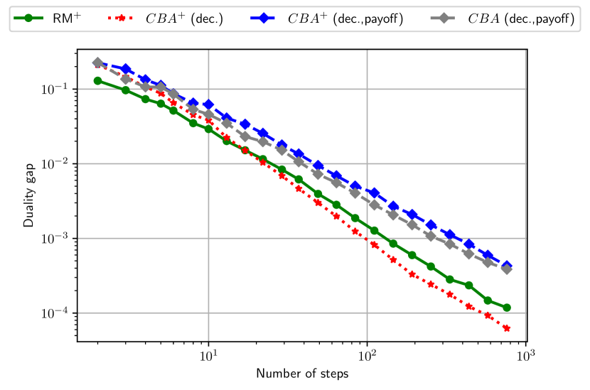
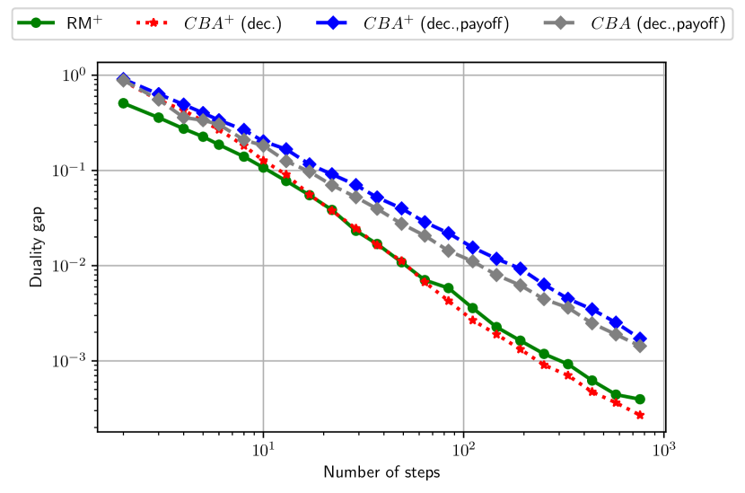
Refer to caption
(a) Uniform distribution.
Refer to caption
(b) Normal distribution.
Figure 4: Comparison of RM+ vs. CBA+ and CBA with different linear averaging schemes: only on decisions (CBA+ (dec.)), or on both the decisions and the payoffs 𝒖𝒖\bm{u} (CBA+ (dec.,payoff),CBA (dec.,payoff)).

B.1 Geometric intuition on the projection step of CBA+

Figure 5 illustrates the projection step π𝒞()subscript𝜋𝒞\pi_{\mathcal{C}}(\cdot) of 𝖢𝖡𝖠+𝖢𝖡𝖠+{\sf CBA\textsuperscript{+}}. At a high level, from 𝒖tsubscript𝒖𝑡\bm{u}_{t} to 𝒖t+1subscript𝒖𝑡1\bm{u}_{t+1}, an instantaneous payoff 𝒗tsubscript𝒗𝑡\bm{v}_{t} is first added to 𝒖tsubscript𝒖𝑡\bm{u}_{t} (where 𝒗t=(𝒇t,𝒙t/κ,𝒇t)\bm{v}_{t}=\left(\langle\bm{f}_{t},\bm{x}_{t}\rangle/\kappa,-\bm{f}_{t}\rangle\right)), and then the resulting vector 𝒖t+=𝒖t+𝒗tsubscriptsuperscript𝒖𝑡subscript𝒖𝑡subscript𝒗𝑡\bm{u}^{+}_{t}=\bm{u}_{t}+\bm{v}_{t} is projected onto 𝒞𝒞\mathcal{C}. The projection π𝒞()subscript𝜋𝒞\pi_{\mathcal{C}}(\cdot) moves the vector 𝒖t+subscriptsuperscript𝒖𝑡\bm{u}^{+}_{t} along the edges of the cone 𝒞superscript𝒞\mathcal{C}^{\circ}, preserving the (orthogonal) distance d𝑑d to 𝒞superscript𝒞\mathcal{C}^{\circ}.

Refer to caption
Refer to caption
Figure 5: Illustration of π𝒞()subscript𝜋𝒞\pi_{\mathcal{C}}(\cdot) for 𝒞=+2𝒞superscriptsubscript2\mathcal{C}=\mathbb{R}_{+}^{2} (left-hand side) and 𝒞𝒞\mathcal{C} any cone in 2superscript2\mathbb{R}^{2} (right-hand side).

Appendix C Proof of Theorem 3.2

Let ωt=t,ST=t=1Tωt=T(T+1)/2formulae-sequencesubscript𝜔𝑡𝑡subscript𝑆𝑇superscriptsubscript𝑡1𝑇subscript𝜔𝑡𝑇𝑇12\omega_{t}=t,S_{T}=\sum_{t=1}^{T}\omega_{t}=T(T+1)/2, and

𝒙¯T=1STt=1Tωt𝒙t,𝒚¯T=1STt=1Tωt𝒚t.formulae-sequencesubscript¯𝒙𝑇1subscript𝑆𝑇superscriptsubscript𝑡1𝑇subscript𝜔𝑡subscript𝒙𝑡subscript¯𝒚𝑇1subscript𝑆𝑇superscriptsubscript𝑡1𝑇subscript𝜔𝑡subscript𝒚𝑡\bar{\bm{x}}_{T}=\frac{1}{S_{T}}\sum_{t=1}^{T}\omega_{t}\bm{x}_{t},\bar{\bm{y}}_{T}=\frac{1}{S_{T}}\sum_{t=1}^{T}\omega_{t}\bm{y}_{t}.

Since F𝐹F is convex-concave, we first have

max𝒚𝒴F(𝒙¯T,𝒚)min𝒙𝒳F(𝒙,𝒚¯T)2T(T+1)(max𝒚𝒴t=1TωtF(𝒙t,𝒚)min𝒙𝒳t=1TωtF(𝒙,𝒚t)).subscript𝒚𝒴𝐹subscript¯𝒙𝑇𝒚subscript𝒙𝒳𝐹𝒙subscript¯𝒚𝑇2𝑇𝑇1subscript𝒚𝒴superscriptsubscript𝑡1𝑇subscript𝜔𝑡𝐹subscript𝒙𝑡𝒚subscript𝒙𝒳superscriptsubscript𝑡1𝑇subscript𝜔𝑡𝐹𝒙subscript𝒚𝑡\max_{\bm{y}\in\mathcal{Y}}F(\bar{\bm{x}}_{T},\bm{y})-\min_{\bm{x}\in\mathcal{X}}F(\bm{x},\bar{\bm{y}}_{T})\leq\frac{2}{T(T+1)}\left(\max_{\bm{y}\in\mathcal{Y}}\sum_{t=1}^{T}\omega_{t}F(\bm{x}_{t},\bm{y})-\min_{\bm{x}\in\mathcal{X}}\sum_{t=1}^{T}\omega_{t}F(\bm{x},\bm{y}_{t})\right).

Now,

max𝒚𝒴t=1TωtF(𝒙t,𝒚)min𝒙𝒳t=1TωtF(𝒙,𝒚t)subscript𝒚𝒴superscriptsubscript𝑡1𝑇subscript𝜔𝑡𝐹subscript𝒙𝑡𝒚subscript𝒙𝒳superscriptsubscript𝑡1𝑇subscript𝜔𝑡𝐹𝒙subscript𝒚𝑡\displaystyle\max_{\bm{y}\in\mathcal{Y}}\sum_{t=1}^{T}\omega_{t}F(\bm{x}_{t},\bm{y})-\min_{\bm{x}\in\mathcal{X}}\sum_{t=1}^{T}\omega_{t}F(\bm{x},\bm{y}_{t}) =(max𝒚𝒴t=1TωtF(𝒙t,𝒚)t=1TωtF(𝒙t,𝒚t))absentsubscript𝒚𝒴superscriptsubscript𝑡1𝑇subscript𝜔𝑡𝐹subscript𝒙𝑡𝒚superscriptsubscript𝑡1𝑇subscript𝜔𝑡𝐹subscript𝒙𝑡subscript𝒚𝑡\displaystyle=\left(\max_{\bm{y}\in\mathcal{Y}}\sum_{t=1}^{T}\omega_{t}F(\bm{x}_{t},\bm{y})-\sum_{t=1}^{T}\omega_{t}F(\bm{x}_{t},\bm{y}_{t})\right)
+(t=1TωtF(𝒙t,𝒚t)min𝒙𝒳t=1TωtF(𝒙,𝒚t)).superscriptsubscript𝑡1𝑇subscript𝜔𝑡𝐹subscript𝒙𝑡subscript𝒚𝑡subscript𝒙𝒳superscriptsubscript𝑡1𝑇subscript𝜔𝑡𝐹𝒙subscript𝒚𝑡\displaystyle+\left(\sum_{t=1}^{T}\omega_{t}F(\bm{x}_{t},\bm{y}_{t})-\min_{\bm{x}\in\mathcal{X}}\sum_{t=1}^{T}\omega_{t}F(\bm{x},\bm{y}_{t})\right).

Now since F𝐹F is convex-concave, we can use the following upper bound:

max𝒚𝒴t=1TωtF(𝒙t,𝒚)t=1TωtF(𝒙t,𝒚t)subscript𝒚𝒴superscriptsubscript𝑡1𝑇subscript𝜔𝑡𝐹subscript𝒙𝑡𝒚superscriptsubscript𝑡1𝑇subscript𝜔𝑡𝐹subscript𝒙𝑡subscript𝒚𝑡\displaystyle\max_{\bm{y}\in\mathcal{Y}}\sum_{t=1}^{T}\omega_{t}F(\bm{x}_{t},\bm{y})-\sum_{t=1}^{T}\omega_{t}F(\bm{x}_{t},\bm{y}_{t}) max𝒚𝒴ωtt=1T𝒈t,𝒚t=1Tωt𝒈t,𝒚t,absentsubscript𝒚𝒴subscript𝜔𝑡superscriptsubscript𝑡1𝑇subscript𝒈𝑡𝒚superscriptsubscript𝑡1𝑇subscript𝜔𝑡subscript𝒈𝑡subscript𝒚𝑡\displaystyle\leq\max_{\bm{y}\in\mathcal{Y}}\omega_{t}\sum_{t=1}^{T}\langle\bm{g}_{t},\bm{y}\rangle-\sum_{t=1}^{T}\omega_{t}\langle\bm{g}_{t},\bm{y}_{t}\rangle,
t=1TωtF(𝒙t,𝒚t)min𝒙𝒳t=1TωtF(𝒙,𝒚t)superscriptsubscript𝑡1𝑇subscript𝜔𝑡𝐹subscript𝒙𝑡subscript𝒚𝑡subscript𝒙𝒳superscriptsubscript𝑡1𝑇subscript𝜔𝑡𝐹𝒙subscript𝒚𝑡\displaystyle\sum_{t=1}^{T}\omega_{t}F(\bm{x}_{t},\bm{y}_{t})-\min_{\bm{x}\in\mathcal{X}}\sum_{t=1}^{T}\omega_{t}F(\bm{x},\bm{y}_{t}) t=1Tωt𝒇t,𝒙tmin𝒙𝒳t=1Tωt𝒇t,𝒙,absentsuperscriptsubscript𝑡1𝑇subscript𝜔𝑡subscript𝒇𝑡subscript𝒙𝑡subscript𝒙𝒳superscriptsubscript𝑡1𝑇subscript𝜔𝑡subscript𝒇𝑡𝒙\displaystyle\leq\sum_{t=1}^{T}\omega_{t}\langle\bm{f}_{t},\bm{x}_{t}\rangle-\min_{\bm{x}\in\mathcal{X}}\sum_{t=1}^{T}\omega_{t}\langle\bm{f}_{t},\bm{x}\rangle,

where 𝒇t𝒙F(𝒙t,𝒚t),𝒈t𝒚F(𝒙t,𝒚t)formulae-sequencesubscript𝒇𝑡subscript𝒙𝐹subscript𝒙𝑡subscript𝒚𝑡subscript𝒈𝑡subscript𝒚𝐹subscript𝒙𝑡subscript𝒚𝑡\bm{f}_{t}\in\partial_{\bm{x}}F(\bm{x}_{t},\bm{y}_{t}),\bm{g}_{t}\in\partial_{\bm{y}}F(\bm{x}_{t},\bm{y}_{t}) (recall the repeated game framework presented at the beginning of Section 2).

Now we have proved in Theorem 3.1 that

2T(T+1)max𝒚𝒴t=1Tωt𝒈t,𝒚t=1Tωt𝒈t,𝒚t2𝑇𝑇1subscript𝒚𝒴superscriptsubscript𝑡1𝑇subscript𝜔𝑡subscript𝒈𝑡𝒚superscriptsubscript𝑡1𝑇subscript𝜔𝑡subscript𝒈𝑡subscript𝒚𝑡\displaystyle\frac{2}{T(T+1)}\max_{\bm{y}\in\mathcal{Y}}\sum_{t=1}^{T}\omega_{t}\langle\bm{g}_{t},\bm{y}\rangle-\sum_{t=1}^{T}\langle\omega_{t}\bm{g}_{t},\bm{y}_{t}\rangle =O(κL/T),absent𝑂𝜅𝐿𝑇\displaystyle=O\left(\kappa L/\sqrt{T}\right),
2T(T+1)t=1Tωt𝒇t,𝒙tmin𝒙𝒳t=1Tωt𝒇t,𝒙2𝑇𝑇1superscriptsubscript𝑡1𝑇subscript𝜔𝑡subscript𝒇𝑡subscript𝒙𝑡subscript𝒙𝒳superscriptsubscript𝑡1𝑇subscript𝜔𝑡subscript𝒇𝑡𝒙\displaystyle\frac{2}{T(T+1)}\sum_{t=1}^{T}\omega_{t}\langle\bm{f}_{t},\bm{x}_{t}\rangle-\min_{\bm{x}\in\mathcal{X}}\sum_{t=1}^{T}\omega_{t}\langle\bm{f}_{t},\bm{x}\rangle =O(κL/T).absent𝑂𝜅𝐿𝑇\displaystyle=O\left(\kappa L/\sqrt{T}\right).

Therefore, we can conclude that

max𝒚𝒴F(𝒙¯T,𝒚)min𝒙𝒳F(𝒙,𝒚¯T)=O(κL/T).subscript𝒚𝒴𝐹subscript¯𝒙𝑇𝒚subscript𝒙𝒳𝐹𝒙subscript¯𝒚𝑇𝑂𝜅𝐿𝑇\max_{\bm{y}\in\mathcal{Y}}F(\bar{\bm{x}}_{T},\bm{y})-\min_{\bm{x}\in\mathcal{X}}F(\bm{x},\bar{\bm{y}}_{T})=O\left(\kappa L/\sqrt{T}\right).
Remark C.1.

Note that we essentially reprove the folk theorem, except that we consider weighted average for the decisions of both players. This is because Theorem 3.2 uses linear averaging on decisions, whereas Theorem 2.1 is written with uniform averaging on decisions.

Appendix D Proofs of the projections of Section 3.1

We will extensively use Moreau’s Decomposition Theorem (Combettes and Reyes, 2013): for any convex cone 𝒞n+1𝒞superscript𝑛1\mathcal{C}\subset\mathbb{R}^{n+1} and 𝒖n+1𝒖superscript𝑛1\bm{u}\in\mathbb{R}^{n+1}, we can decompose 𝒖=π𝒞(𝒖)+π𝒞(𝒖)𝒖subscript𝜋𝒞𝒖subscript𝜋superscript𝒞𝒖\bm{u}=\pi_{\mathcal{C}}(\bm{u})+\pi_{\mathcal{C}^{\circ}}(\bm{u}), where 𝒞superscript𝒞\mathcal{C}^{\circ} is the polar cone of 𝒞𝒞\mathcal{C}. Therefore, to compute π𝒞(𝒖)subscript𝜋𝒞𝒖\pi_{\mathcal{C}}(\bm{u}), it is sufficient to compute π𝒞(𝒖)subscript𝜋superscript𝒞𝒖\pi_{\mathcal{C}^{\circ}}(\bm{u}), the orthogonal projection of 𝒖𝒖\bm{u} onto 𝒞superscript𝒞\mathcal{C}^{\circ}. We will see that in some cases, it is simpler to compute π𝒞(𝒖)subscript𝜋superscript𝒞𝒖\pi_{\mathcal{C}^{\circ}}(\bm{u}) and then use π𝒞(𝒖)=𝒖πC(𝒖)subscript𝜋𝒞𝒖𝒖subscript𝜋superscript𝐶𝒖\pi_{\mathcal{C}}(\bm{u})=\bm{u}-\pi_{C^{\circ}}(\bm{u}) than directly computing πC(𝒖)subscript𝜋𝐶𝒖\pi_{C}(\bm{u}) via solving (4).

D.1 The case of the simplex

We consider 𝒳=Δ(n)𝒳Δ𝑛\mathcal{X}=\Delta(n). Note that in this case, κ=max𝒙Δ(n)𝒙2=1𝜅subscript𝒙Δ𝑛subscriptnorm𝒙21\kappa=\max_{\bm{x}\in\Delta(n)}\|\bm{x}\|_{2}=1. The next lemma gives a closed-form expression of 𝒞superscript𝒞\mathcal{C}^{\circ}.

Lemma D.1.

Let 𝒞=cone({1}×Δ(n))𝒞cone1Δ𝑛\mathcal{C}=\textrm{cone}(\{1\}\times\Delta(n)). Then 𝒞={(y~,𝐲^)n+1|maxi=1,,ny^iy~}.superscript𝒞conditional-set~𝑦^𝐲superscript𝑛1subscript𝑖1𝑛subscript^𝑦𝑖~𝑦\mathcal{C}^{\circ}=\{(\tilde{y},\hat{\bm{y}})\in\mathbb{R}^{n+1}\;|\;\max_{i=1,...,n}\hat{y}_{i}\leq-\tilde{y}\}.

Proof of Lemma D.1.

Note that for 𝒚=(y~,𝒚^)n+1𝒚~𝑦^𝒚superscript𝑛1\bm{y}=(\tilde{y},\hat{\bm{y}})\in\mathbb{R}^{n+1} we have

𝒚𝒞𝒚superscript𝒞\displaystyle\bm{y}\in\mathcal{C}^{\circ} 𝒚,𝒛0,𝒛𝒞iffabsentformulae-sequence𝒚𝒛0for-all𝒛𝒞\displaystyle\iff\langle\bm{y},\bm{z}\rangle\leq 0,\forall\;\bm{z}\in\mathcal{C}
(y~,𝒚^),α(1,𝒙)0,𝒙Δ(n),α0iffabsentformulae-sequence~𝑦^𝒚𝛼1𝒙0formulae-sequencefor-all𝒙Δ𝑛for-all𝛼0\displaystyle\iff\langle(\tilde{y},\hat{\bm{y}}),\alpha(1,\bm{x})\rangle\leq 0,\forall\;\bm{x}\in\Delta(n),\forall\;\alpha\geq 0
y~+𝒚^,𝒙0,𝒙Δ(n)iffabsentformulae-sequence~𝑦^𝒚𝒙0for-all𝒙Δ𝑛\displaystyle\iff\tilde{y}+\langle\hat{\bm{y}},\bm{x}\rangle\leq 0,\forall\;\bm{x}\in\Delta(n)
max𝒙Δ(n)𝒚^,𝒙y~iffabsentsubscript𝒙Δ𝑛^𝒚𝒙~𝑦\displaystyle\iff\max_{\bm{x}\in\Delta(n)}\langle\hat{\bm{y}},\bm{x}\rangle\leq-\tilde{y}
maxi=1,,ny^iy~.iffabsentsubscript𝑖1𝑛subscript^𝑦𝑖~𝑦\displaystyle\iff\max_{i=1,...,n}\hat{y}_{i}\leq-\tilde{y}.

For a given 𝒖=(u~,𝒖^)𝒖~𝑢^𝒖\bm{u}=\left(\tilde{u},\hat{\bm{u}}\right), computing π𝒞(𝒖)subscript𝜋superscript𝒞𝒖\pi_{\mathcal{C}^{\circ}}(\bm{u}) is now equivalent to solving

min{(y~u~)2+𝒚^𝒖^22|(y~,𝒚^)n+1,maxi=1,,ny^iy~}.superscript~𝑦~𝑢2conditionalsuperscriptsubscriptnorm^𝒚^𝒖22~𝑦^𝒚superscript𝑛1subscript𝑖1𝑛subscript^𝑦𝑖~𝑦\min\{(\tilde{y}-\tilde{u})^{2}+\|\hat{\bm{y}}-\hat{\bm{u}}\|_{2}^{2}\;|\;(\tilde{y},\hat{\bm{y}})\in\mathbb{R}^{n+1},\max_{i=1,...,n}\hat{y}_{i}\leq-\tilde{y}\}. (18)

Using the reformulation (18), we show that for a fixed y~~𝑦\tilde{y}, the optimal 𝒚^(y~)^𝒚~𝑦\hat{\bm{y}}(\tilde{y}) can be computed in closed-form. It is then possible to avoid a binary search over y~~𝑦\tilde{y} and to simply use a sorting algorithm to obtain the optimal y~~𝑦\tilde{y}. The next proposition summarizes our complexity result for 𝒳=Δ(n)𝒳Δ𝑛\mathcal{X}=\Delta(n).

Proposition D.2.

An optimal solution π𝒞(𝐮)subscript𝜋superscript𝒞𝐮\pi_{\mathcal{C}^{\circ}}(\bm{u}) to (18) can be computed in O(nlog(n))𝑂𝑛𝑛O(n\log(n)) time.

Proof.

Computing π𝒞(𝒖)subscript𝜋superscript𝒞𝒖\pi_{\mathcal{C}^{\circ}}(\bm{u}) is equivalent to computing

min\displaystyle\min\; (y~u~)2+𝒚^𝒖^22superscript~𝑦~𝑢2superscriptsubscriptnorm^𝒚^𝒖22\displaystyle(\tilde{y}-\tilde{u})^{2}+\|\hat{\bm{y}}-\hat{\bm{u}}\|_{2}^{2}
y~,𝒚^n,formulae-sequence~𝑦^𝒚superscript𝑛\displaystyle\tilde{y}\in\mathbb{R},\hat{\bm{y}}\in\mathbb{R}^{n},
maxi=1,,ny^iy~.subscript𝑖1𝑛subscript^𝑦𝑖~𝑦\displaystyle\max_{i=1,...,n}\hat{y}_{i}\leq-\tilde{y}.

Let us fix y~~𝑦\tilde{y}\in\mathbb{R} and let us first solve

min\displaystyle\min 𝒚^𝒖^22superscriptsubscriptnorm^𝒚^𝒖22\displaystyle\|\hat{\bm{y}}-\hat{\bm{u}}\|_{2}^{2} (19)
𝒚^n,^𝒚superscript𝑛\displaystyle\hat{\bm{y}}\in\mathbb{R}^{n},
maxi=1,,ny^iy~.subscript𝑖1𝑛subscript^𝑦𝑖~𝑦\displaystyle\max_{i=1,...,n}\hat{y}_{i}\leq-\tilde{y}.

This is essentially the projection of 𝒖^^𝒖\hat{\bm{u}} on (,y~]nsuperscript~𝑦𝑛(-\infty,-\tilde{y}]^{n}. So a solution to (19) is y^i(y~)=min{y~,u^i},i=1,,n.formulae-sequencesubscript^𝑦𝑖~𝑦~𝑦subscript^𝑢𝑖for-all𝑖1𝑛\hat{y}_{i}(\tilde{y})=\min\{-\tilde{y},\hat{u}_{i}\},\forall\;i=1,...,n. Note that in this case we have 𝒖^𝒚^(y~)=(𝒖^+y~𝒆)+.^𝒖^𝒚~𝑦superscript^𝒖~𝑦𝒆\hat{\bm{u}}-\hat{\bm{y}}(\tilde{y})=\left(\hat{\bm{u}}+\tilde{y}\bm{e}\right)^{+}. So overall the projection brings down to the optimization of ϕ:+:italic-ϕmaps-tosubscript\phi:\mathbb{R}\mapsto\mathbb{R}_{+} such that

ϕ:y~(y~u~)2+(𝒖^+y~𝒆)+22.:italic-ϕmaps-to~𝑦superscript~𝑦~𝑢2superscriptsubscriptnormsuperscript^𝒖~𝑦𝒆22\phi:\tilde{y}\mapsto(\tilde{y}-\tilde{u})^{2}+\|\left(\hat{\bm{u}}+\tilde{y}\bm{e}\right)^{+}\|_{2}^{2}. (20)

In principle, we could use binary search with a doubling trick to compute a ϵitalic-ϵ\epsilon-minimizer of the convex function ϕitalic-ϕ\phi in O(log(ϵ1))𝑂superscriptitalic-ϵ1O\left(\log(\epsilon^{-1})\right) calls to ϕitalic-ϕ\phi. However, it is possible to a minimizer y~superscript~𝑦\tilde{y}^{*} of ϕitalic-ϕ\phi using the following remark. By construction, we know that 𝒖π𝒞(𝒖)𝒞𝒖subscript𝜋superscript𝒞𝒖𝒞\bm{u}-\pi_{\mathcal{C}^{\circ}}(\bm{u})\in\mathcal{C}. Here, 𝒞=cone({1}×Δ(n))𝒞cone1Δ𝑛\mathcal{C}=\textrm{cone}\left(\{1\}\times\Delta(n)\right), and 𝒖π𝒞(𝒖)=(u~y~,(𝒖^+y~𝒆)+).𝒖subscript𝜋superscript𝒞𝒖~𝑢superscript~𝑦superscript^𝒖superscript~𝑦𝒆\bm{u}-\pi_{\mathcal{C}^{\circ}}(\bm{u})=\left(\tilde{u}-\tilde{y}^{*},\left(\hat{\bm{u}}+\tilde{y}^{*}\bm{e}\right)^{+}\right). This proves that

(𝒖^+y~𝒆)+u~y~Δ(n),superscript^𝒖superscript~𝑦𝒆~𝑢superscript~𝑦Δ𝑛\dfrac{\left(\hat{\bm{u}}+\tilde{y}^{*}\bm{e}\right)^{+}}{\tilde{u}-\tilde{y}^{*}}\in\Delta(n),

which in turns imply that

y~+i=1nmax{u^i+y~,0}=u~.superscript~𝑦superscriptsubscript𝑖1𝑛subscript^𝑢𝑖superscript~𝑦0~𝑢\tilde{y}^{*}+\sum_{i=1}^{n}\max\{\hat{u}_{i}+\tilde{y}^{*},0\}=\tilde{u}. (21)

We can use (21) to efficiently compute y~superscript~𝑦\tilde{y}^{*} without using any binary search. In particular, we can sort the coefficients of 𝒖^^𝒖\hat{\bm{u}} in O(nlog(n))𝑂𝑛𝑛O\left(n\log(n)\right) operations, and use (21) to find y~superscript~𝑦\tilde{y}^{*}. ∎

Having obtained π𝒞(𝒖)subscript𝜋superscript𝒞𝒖\pi_{\mathcal{C}^{\circ}}(\bm{u}), we can obtain π𝒞(𝒖)subscript𝜋𝒞𝒖\pi_{\mathcal{C}}(\bm{u}) by using the identity π𝒞(𝒖)=𝒖π𝒞(𝒖)subscript𝜋𝒞𝒖𝒖subscript𝜋superscript𝒞𝒖\pi_{\mathcal{C}}(\bm{u})=\bm{u}-\pi_{\mathcal{C}^{\circ}}(\bm{u}). Note that RM and RM+ are obtained by choosing the closed-form feasible point corresponding to y~=u~~𝑦~𝑢\tilde{y}=\tilde{u} in (18).

D.2 The case of an psubscript𝑝\ell_{p} ball

In this section we assume that 𝒳={𝒙n|;𝒙p1}\mathcal{X}=\{\bm{x}\in\mathbb{R}^{n}\;|\ ;\|\bm{x}\|_{p}\leq 1\} with p1𝑝1p\geq 1 or p=𝑝p=\infty. The next lemma provides a closed-form reformulation of the polar cone 𝒞superscript𝒞\mathcal{C}^{\circ}.

Lemma D.3.

Let 𝒳={𝐱n|;𝐱p1},\mathcal{X}=\{\bm{x}\in\mathbb{R}^{n}\;|\ ;\|\bm{x}\|_{p}\leq 1\}, with p1𝑝1p\geq 1 or p=𝑝p=\infty. Then 𝒞={(y~,𝐲)×n|𝐲qy~}superscript𝒞conditional-set~𝑦𝐲superscript𝑛subscriptnorm𝐲𝑞~𝑦\mathcal{C}^{\circ}=\{(\tilde{y},\bm{y})\in\mathbb{R}\times\mathbb{R}^{n}\;|\;\|\bm{y}\|_{q}\leq-\tilde{y}\}, with q𝑞q such that 1/p+1/q=11𝑝1𝑞11/p+1/q=1.

Proof of Lemma D.3.

Let us write Bp(1)={𝒛n|𝒛p1}subscript𝐵𝑝1conditional-set𝒛superscript𝑛subscriptnorm𝒛𝑝1B_{p}(1)=\{\bm{z}\in\mathbb{R}^{n}\;|\;\|\bm{z}\|_{p}\leq 1\}. Note that for 𝒚=(y~,𝒚^)n+1𝒚~𝑦^𝒚superscript𝑛1\bm{y}=(\tilde{y},\hat{\bm{y}})\in\mathbb{R}^{n+1} we have

𝒚𝒞𝒚superscript𝒞\displaystyle\bm{y}\in\mathcal{C}^{\circ} 𝒚,𝒛0,𝒛𝒞iffabsentformulae-sequence𝒚𝒛0for-all𝒛𝒞\displaystyle\iff\langle\bm{y},\bm{z}\rangle\leq 0,\forall\;\bm{z}\in\mathcal{C}
(y~,𝒚^),α(1,𝒙)0,𝒙Bp(1),α0iffabsentformulae-sequence~𝑦^𝒚𝛼1𝒙0formulae-sequencefor-all𝒙subscript𝐵𝑝1for-all𝛼0\displaystyle\iff\langle(\tilde{y},\hat{\bm{y}}),\alpha(1,\bm{x})\rangle\leq 0,\forall\;\bm{x}\in B_{p}(1),\forall\;\alpha\geq 0
y~+𝒚^,𝒙0,𝒙Bp(1),iffabsentformulae-sequence~𝑦^𝒚𝒙0for-all𝒙subscript𝐵𝑝1\displaystyle\iff\tilde{y}+\langle\hat{\bm{y}},\bm{x}\rangle\leq 0,\forall\;\bm{x}\in B_{p}(1),
max𝒙Bp(1),𝒚^,𝒙y~iffabsentsubscript𝒙subscript𝐵𝑝1^𝒚𝒙~𝑦\displaystyle\iff\max_{\bm{x}\in B_{p}(1),}\langle\hat{\bm{y}},\bm{x}\rangle\leq-\tilde{y}
𝒙qy~,iffabsentsubscriptnorm𝒙𝑞~𝑦\displaystyle\iff\|\bm{x}\|_{q}\leq-\tilde{y},

since q\|\cdot\|_{q} is the dual norm of p\|\cdot\|_{p}. ∎

The orthogonal projection problem onto 𝒞superscript𝒞\mathcal{C}^{\circ} becomes

min{(y~u~)2+𝒚^𝒖^22|(y~,𝒚^)n+1,𝒚^qy~}.superscript~𝑦~𝑢2conditionalsuperscriptsubscriptnorm^𝒚^𝒖22~𝑦^𝒚superscript𝑛1subscriptnorm^𝒚𝑞~𝑦\min\{(\tilde{y}-\tilde{u})^{2}+\|\hat{\bm{y}}-\hat{\bm{u}}\|_{2}^{2}\;|\;(\tilde{y},\hat{\bm{y}})\in\mathbb{R}^{n+1},\|\hat{\bm{y}}\|_{q}\leq-\tilde{y}\}. (22)

For p=2𝑝2p=2, (22) has a closed-form solution. For p=1𝑝1p=1, a quasi-closed-form solution to (22) can be obtained efficiently using sorting. For p=𝑝p=\infty, it is more efficient to directly compute π𝒞(𝒖)subscript𝜋𝒞𝒖\pi_{\mathcal{C}}(\bm{u}). This is because the dual norm of \|\cdot\|_{\infty} is 1\|\cdot\|_{1}.

Proposition D.4.
  • For p=1𝑝1p=1, π𝒞(𝒖)subscript𝜋superscript𝒞𝒖\pi_{\mathcal{C}^{\circ}}(\bm{u}) can be computed in O(nlog(n))𝑂𝑛𝑛O(n\log(n)) arithmetic operations.

  • For p=𝑝p=\infty, π𝒞(𝒖)subscript𝜋𝒞𝒖\pi_{\mathcal{C}}(\bm{u}) can be computed in O(nlog(n))𝑂𝑛𝑛O(n\log(n)) arithmetic operations.

  • For p=2𝑝2p=2, π𝒞(𝒖)subscript𝜋𝒞𝒖\pi_{\mathcal{C}}(\bm{u}) can be computed in closed-form.

Proof.

The case p=1𝑝1p=1. Assume that p=1𝑝1p=1. Then q=\|\cdot\|_{q}=\|\cdot\|_{\infty}. We want to compute the projection of (u~,𝒖^)~𝑢^𝒖\left(\tilde{u},\hat{\bm{u}}\right) on 𝒞superscript𝒞\mathcal{C}^{\circ}:

min𝒚𝒞𝒚𝒖22=minsubscript𝒚superscript𝒞superscriptsubscriptnorm𝒚𝒖22\displaystyle\min_{\bm{y}\in\mathcal{C}^{\circ}}\|\bm{y}-\bm{u}\|_{2}^{2}=\min (y~u~)2+𝒚^𝒖^22superscript~𝑦~𝑢2superscriptsubscriptnorm^𝒚^𝒖22\displaystyle\;(\tilde{y}-\tilde{u})^{2}+\|\hat{\bm{y}}-\hat{\bm{u}}\|_{2}^{2} (23)
y~,𝒚^n,formulae-sequence~𝑦^𝒚superscript𝑛\displaystyle\;\tilde{y}\in\mathbb{R},\hat{\bm{y}}\in\mathbb{R}^{n},
𝒚^y~.subscriptnorm^𝒚~𝑦\displaystyle\|\hat{\bm{y}}\|_{\infty}\leq-\tilde{y}.

For a fixed y~~𝑦\tilde{y}, we want to compute

min\displaystyle\min 𝒚^𝒖^22superscriptsubscriptnorm^𝒚^𝒖22\displaystyle\;\|\hat{\bm{y}}-\hat{\bm{u}}\|_{2}^{2} (24)
𝒚^n,^𝒚superscript𝑛\displaystyle\hat{\bm{y}}\in\mathbb{R}^{n},
𝒚^y~.subscriptnorm^𝒚~𝑦\displaystyle\|\hat{\bm{y}}\|_{\infty}\leq-\tilde{y}.

The projection (24) can be computed in closed-form as

𝒚^(y~)=min{y~,max{y~,𝒖^}}superscript^𝒚~𝑦~𝑦~𝑦^𝒖\hat{\bm{y}}^{*}(\tilde{y})=\min\{-\tilde{y},\max\{\tilde{y},\hat{\bm{u}}\}\} (25)

since this is simply the orthogonal projection of 𝒖^^𝒖\hat{\bm{u}} onto the subscript\ell_{\infty} ball of radius y~~𝑦-\tilde{y}. Let us call ϕ::italic-ϕmaps-to\phi:\mathbb{R}\mapsto\mathbb{R} such that

ϕ(y~)=(y~u~)2+𝒚^(y~)𝒖^22.italic-ϕ~𝑦superscript~𝑦~𝑢2superscriptsubscriptnormsuperscript^𝒚~𝑦^𝒖22\phi(\tilde{y})=\left(\tilde{y}-\tilde{u}\right)^{2}+\|\hat{\bm{y}}^{*}(\tilde{y})-\hat{\bm{u}}\|_{2}^{2}.

Because of the closed-form expression for 𝒚^(y~)superscript^𝒚~𝑦\hat{\bm{y}}^{*}(\tilde{y}) as in (25), we have

ϕ:y~(y~u~)2+(𝒖^+y~𝒆)+22.:italic-ϕmaps-to~𝑦superscript~𝑦~𝑢2superscriptsubscriptnormsuperscript^𝒖~𝑦𝒆22\phi:\tilde{y}\mapsto\left(\tilde{y}-\tilde{u}\right)^{2}+\|\left(\hat{\bm{u}}+\tilde{y}\bm{e}\right)^{+}\|_{2}^{2}.

Finding a minimizer of ϕitalic-ϕ\phi can be done in O(nlog(n))𝑂𝑛𝑛O(n\log(n)), with the same methods as in the proof in the previous section (Appendix D.1).

The case p=𝑝p=\infty. Let p=𝑝p=\infty. The problem of computing π𝒞(𝒖)subscript𝜋𝒞𝒖\pi_{\mathcal{C}}(\bm{u}), the orthogonal projection onto the cone 𝒞𝒞\mathcal{C}, is equivalent to

min𝒚𝒞𝒚𝒖22=minsubscript𝒚superscript𝒞superscriptsubscriptnorm𝒚𝒖22\displaystyle\min_{\bm{y}\in\mathcal{C}^{\circ}}\|\bm{y}-\bm{u}\|_{2}^{2}=\min (y~u~)2+𝒚^𝒖^22superscript~𝑦~𝑢2superscriptsubscriptnorm^𝒚^𝒖22\displaystyle\;(\tilde{y}-\tilde{u})^{2}+\|\hat{\bm{y}}-\hat{\bm{u}}\|_{2}^{2} (26)
y~,𝒚^n,formulae-sequence~𝑦^𝒚superscript𝑛\displaystyle\;\tilde{y}\in\mathbb{R},\hat{\bm{y}}\in\mathbb{R}^{n},
𝒚^y~.subscriptnorm^𝒚~𝑦\displaystyle\|\hat{\bm{y}}\|_{\infty}\leq\tilde{y}.

Note the similarity between (26) (computing the orthogonal projection onto 𝒞𝒞\mathcal{C} when p=𝑝p=\infty), and (23) (computing the orthogonal projection onto 𝒞superscript𝒞\mathcal{C}^{\circ} when p=1𝑝1p=1). From Lemma D.3, we know that this is the case because 1\|\cdot\|_{1} and \|\cdot\|_{\infty} are dual norms to each other.

Therefore, the methods described for computing π𝒞(𝒖)subscript𝜋superscript𝒞𝒖\pi_{\mathcal{C}^{\circ}}(\bm{u}) for p=1𝑝1p=1 can be applied to the case p=𝑝p=\infty for directly computing π𝒞(𝒖)subscript𝜋𝒞𝒖\pi_{\mathcal{C}}(\bm{u}). This gives the complexity results as stated in Proposition D.4: π𝒞(𝒖)subscript𝜋𝒞𝒖\pi_{\mathcal{C}}(\bm{u}) can be computed in O(nlog(n))𝑂𝑛𝑛O(n\log(n)) operations.

The case p=2𝑝2p=2. Let p=2\|\cdot\|_{p}=\|\cdot\|_{2}, then q=2\|\cdot\|_{q}=\|\cdot\|_{2}. Let us fix y~~𝑦\tilde{y} and consider solving

min\displaystyle\min 𝒚^𝒖^22superscriptsubscriptnorm^𝒚^𝒖22\displaystyle\;\|\hat{\bm{y}}-\hat{\bm{u}}\|_{2}^{2} (27)
𝒚^n,^𝒚superscript𝑛\displaystyle\hat{\bm{y}}\in\mathbb{R}^{n},
𝒚^2y~.subscriptnorm^𝒚2~𝑦\displaystyle\|\hat{\bm{y}}\|_{2}\leq-\tilde{y}.

The projection (27) can be computed in closed-form as

𝒚^(y~)=(y~)𝒖^𝒖^2,superscript^𝒚~𝑦~𝑦^𝒖subscriptnorm^𝒖2\hat{\bm{y}}^{*}(\tilde{y})=\left(-\tilde{y}\right)\dfrac{\hat{\bm{u}}}{\|\hat{\bm{u}}\|_{2}},

since this is just the orthogonal projection of the vector 𝒖^^𝒖\hat{\bm{u}} onto the 2subscript2\ell_{2}-ball of radius y~~𝑦-\tilde{y}. Let us call ϕ::italic-ϕmaps-to\phi:\mathbb{R}\mapsto\mathbb{R} such that

ϕ(y~)=(y~u~)2+𝒚^(y~)𝒖^22.italic-ϕ~𝑦superscript~𝑦~𝑢2superscriptsubscriptnormsuperscript^𝒚~𝑦^𝒖22\phi(\tilde{y})=\left(\tilde{y}-\tilde{u}\right)^{2}+\|\hat{\bm{y}}^{*}(\tilde{y})-\hat{\bm{u}}\|_{2}^{2}.

Note that here, y~𝒚^(y~)maps-to~𝑦superscript^𝒚~𝑦\tilde{y}\mapsto\hat{\bm{y}}^{*}(\tilde{y}) is differentiable. Therefore ϕ:y~(y~u~)2+𝒚^(y~)𝒖^22:italic-ϕmaps-to~𝑦superscript~𝑦~𝑢2superscriptsubscriptnormsuperscript^𝒚~𝑦^𝒖22\phi:\tilde{y}\mapsto\left(\tilde{y}-\tilde{u}\right)^{2}+\|\hat{\bm{y}}^{*}(\tilde{y})-\hat{\bm{u}}\|_{2}^{2} is also differentiable. First-order optimality conditions yield a closed-form solution for computing (y~,𝒚^)=π𝒞(𝒖)superscript~𝑦superscript^𝒚subscript𝜋superscript𝒞𝒖(\tilde{y}^{*},\hat{\bm{y}}^{*})=\pi_{\mathcal{C}^{\circ}}(\bm{u}), as

y~=u~𝒖^22,𝒚^=12(u~𝒖^2)𝒖^𝒖^2.formulae-sequencesuperscript~𝑦~𝑢subscriptnorm^𝒖22superscript^𝒚12~𝑢subscriptnorm^𝒖2^𝒖subscriptnorm^𝒖2\tilde{y}^{*}=\dfrac{\tilde{u}-\|\hat{\bm{u}}\|_{2}}{2},\hat{\bm{y}}^{*}=-\dfrac{1}{2}(\tilde{u}-\|\hat{\bm{u}}\|_{2})\frac{\hat{\bm{u}}}{\|\hat{\bm{u}}\|_{2}}. (28)

D.3 The case of an ellipsoidal confidence region in the simplex

In this section we assume that 𝒳𝒳\mathcal{X} is 𝒳={𝒙Δ(n)|𝒙𝒙02ϵx}𝒳conditional-set𝒙Δ𝑛subscriptnorm𝒙subscript𝒙02subscriptitalic-ϵ𝑥\mathcal{X}=\{\bm{x}\in\Delta(n)\;|\;\|\bm{x}-\bm{x}_{0}\|_{2}\leq\epsilon_{x}\}. We also assume that {𝒙n|𝒙𝒆=1}{𝒙n|𝒙𝒙02ϵx}Δ(n)conditional-set𝒙superscript𝑛superscript𝒙top𝒆1conditional-set𝒙superscript𝑛subscriptnorm𝒙subscript𝒙02subscriptitalic-ϵ𝑥Δ𝑛\{\bm{x}\in\mathbb{R}^{n}|\bm{x}^{\top}\bm{e}=1\}\bigcap\{\bm{x}\in\mathbb{R}^{n}\;|\;\|\bm{x}-\bm{x}_{0}\|_{2}\leq\epsilon_{x}\}\subseteq\Delta(n), so that we can write 𝒳=𝒙0+ϵB~,𝒳subscript𝒙0italic-ϵ~𝐵\mathcal{X}=\bm{x}_{0}+\epsilon\tilde{B}, where B~={𝒛n|𝒛𝒆=0,𝒛21}.~𝐵conditional-set𝒛superscript𝑛formulae-sequencesuperscript𝒛top𝒆0subscriptnorm𝒛21\tilde{B}=\{\bm{z}\in\mathbb{R}^{n}\;|\;\bm{z}^{\top}\bm{e}=0,\|\bm{z}\|_{2}\leq 1\}.

Suppose we made a sequence of decisions 𝒙1,,𝒙Tsubscript𝒙1subscript𝒙𝑇\bm{x}_{1},...,\bm{x}_{T}, which can be written as 𝒙t=𝒙0+ϵ𝒛tsubscript𝒙𝑡subscript𝒙0italic-ϵsubscript𝒛𝑡\bm{x}_{t}=\bm{x}_{0}+\epsilon\bm{z}_{t} for 𝒛tB~.subscript𝒛𝑡~𝐵\bm{z}_{t}\in\tilde{B}. Then it is clear that for any sequence of payoffs 𝒇1,,𝒇Tsubscript𝒇1subscript𝒇𝑇\bm{f}_{1},...,\bm{f}_{T}, we have

t=1Tωt𝒇t,𝒙tmin𝒙𝒳t=1Tωt𝒇t,𝒙=ϵx(t=1Tωt𝒇t,𝒛tmin𝒛B~t=1Tωt𝒇t,𝒛).superscriptsubscript𝑡1𝑇subscript𝜔𝑡subscript𝒇𝑡subscript𝒙𝑡subscript𝒙𝒳superscriptsubscript𝑡1𝑇subscript𝜔𝑡subscript𝒇𝑡𝒙subscriptitalic-ϵ𝑥superscriptsubscript𝑡1𝑇subscript𝜔𝑡subscript𝒇𝑡subscript𝒛𝑡subscript𝒛~𝐵superscriptsubscript𝑡1𝑇subscript𝜔𝑡subscript𝒇𝑡𝒛\displaystyle\sum_{t=1}^{T}\omega_{t}\langle\bm{f}_{t},\bm{x}_{t}\rangle-\min_{\bm{x}\in\mathcal{X}}\sum_{t=1}^{T}\omega_{t}\langle\bm{f}_{t},\bm{x}\rangle=\epsilon_{x}\left(\sum_{t=1}^{T}\omega_{t}\langle\bm{f}_{t},\bm{z}_{t}\rangle-\min_{\bm{z}\in\tilde{B}}\sum_{t=1}^{T}\omega_{t}\langle\bm{f}_{t},\bm{z}\rangle\right). (29)

Therefore, if we run CBA+ on the set B~~𝐵\tilde{B} to obtain O(T)𝑂𝑇O\left(\sqrt{T}\right) growth of the right-hand side of (29), we obtain a no-regret algorithm for 𝒳𝒳\mathcal{X}. We now show how to run CBA+ for the set B~~𝐵\tilde{B}. Let 𝒱={𝒗n|𝒗𝒆=0}.𝒱conditional-set𝒗superscript𝑛superscript𝒗top𝒆0\mathcal{V}=\{\bm{v}\in\mathbb{R}^{n}\;|\;\bm{v}^{\top}\bm{e}=0\}. We use the following orthonormal basis of 𝒱𝒱\mathcal{V}: let 𝒗1,,𝒗n1nsubscript𝒗1subscript𝒗𝑛1superscript𝑛\bm{v}_{1},...,\bm{v}_{n-1}\in\mathbb{R}^{n} be the vectors 𝒗i=i/(i+1)(1/i,,1/i,1,0,,0),i=1,,n1,formulae-sequencesubscript𝒗𝑖𝑖𝑖11𝑖1𝑖100for-all𝑖1𝑛1\bm{v}_{i}=\sqrt{i/(i+1)}\left(1/i,...,1/i,-1,0,...,0\right),\forall\;i=1,...,n-1, where the component 1/i1𝑖1/i is repeated i𝑖i times. The vectors 𝒗1,,𝒗n1subscript𝒗1subscript𝒗𝑛1\bm{v}_{1},...,\bm{v}_{n-1} are orthonormal and constitute a basis of 𝒱𝒱\mathcal{V} (Egozcue et al., 2003). Writing 𝑽=(𝒗1,,𝒗n1)n×(n1)𝑽subscript𝒗1subscript𝒗𝑛1superscript𝑛𝑛1\bm{V}=\left(\bm{v}_{1},...,\bm{v}_{n-1}\right)\in\mathbb{R}^{n\times(n-1)}, and noting that 𝑽𝑽=𝑰superscript𝑽top𝑽𝑰\bm{V}^{\top}\bm{V}=\bm{I}, we can write B~={𝑽𝒔|𝒔n1,𝒔21}.~𝐵conditional-set𝑽𝒔formulae-sequence𝒔superscript𝑛1subscriptnorm𝒔21\tilde{B}=\{\bm{Vs}\;|\;\bm{s}\in\mathbb{R}^{n-1},\|\bm{s}\|_{2}\leq 1\}. Now, if 𝒙=𝒙0+ϵx𝒛t𝒙subscript𝒙0subscriptitalic-ϵ𝑥subscript𝒛𝑡\bm{x}=\bm{x}_{0}+\epsilon_{x}\bm{z}_{t} with 𝒛t𝒱subscript𝒛𝑡𝒱\bm{z}_{t}\in\mathcal{V}, we have 𝒛t=𝑽𝒔tsubscript𝒛𝑡𝑽subscript𝒔𝑡\bm{z}_{t}=\bm{Vs}_{t}, for 𝒔tn1subscript𝒔𝑡superscript𝑛1\bm{s}_{t}\in\mathbb{R}^{n-1} and 𝒔21subscriptnorm𝒔21\|\bm{s}\|_{2}\leq 1. Finally,

t=1Tωt𝒇t,𝒙tmin𝒙𝒳t=1Tωt𝒇t,𝒙=ϵx(t=1Tωt𝑽𝒇t,𝒔tmin𝒔n1,𝒔21t=1Tωt𝑽𝒇t,𝒔).superscriptsubscript𝑡1𝑇subscript𝜔𝑡subscript𝒇𝑡subscript𝒙𝑡subscript𝒙𝒳superscriptsubscript𝑡1𝑇subscript𝜔𝑡subscript𝒇𝑡𝒙subscriptitalic-ϵ𝑥superscriptsubscript𝑡1𝑇subscript𝜔𝑡superscript𝑽topsubscript𝒇𝑡subscript𝒔𝑡subscriptformulae-sequence𝒔superscript𝑛1subscriptnorm𝒔21superscriptsubscript𝑡1𝑇subscript𝜔𝑡superscript𝑽topsubscript𝒇𝑡𝒔\displaystyle\sum_{t=1}^{T}\omega_{t}\langle\bm{f}_{t},\bm{x}_{t}\rangle-\min_{\bm{x}\in\mathcal{X}}\sum_{t=1}^{T}\omega_{t}\langle\bm{f}_{t},\bm{x}\rangle=\epsilon_{x}\left(\sum_{t=1}^{T}\omega_{t}\langle\bm{V}^{\top}\bm{f}_{t},\bm{s}_{t}\rangle-\min_{\bm{s}\in\mathbb{R}^{n-1},\|\bm{s}\|_{2}\leq 1}\sum_{t=1}^{T}\omega_{t}\langle\bm{V}^{\top}\bm{f}_{t},\bm{s}\rangle\right). (30)

Therefore, to obtain a regret minimizer for the left-hand side of (30) with observed payoffs (𝒇)t0subscript𝒇𝑡0\left(\bm{f}\right)_{t\geq 0}, we can run CBA+ on the right-hand side, where the decision set is an 2subscript2\ell_{2} ball and the sequence of observed payoffs is (𝑽𝒇t)t0subscriptsuperscript𝑽topsubscript𝒇𝑡𝑡0\left(\bm{V}^{\top}\bm{f}_{t}\right)_{t\geq 0}. In the previous section we showed how to efficiently instantiate CBA+ in this setting (see Proposition D.4).

Remark D.5.

In this section we have highlighted a sequence of reformulations of the regret, from (29) to (30). We essentially showed how to instantiate CBA+ for settings where the decision set 𝒳𝒳\mathcal{X} is the intersection of an 2subscript2\ell_{2} ball with a hyperplane for which we have an orthonormal basis.

Appendix E Additional details and numerical experiments for matrix games and EFGs

E.1 Numerical setup

Numerical setup for matrix games

For the experiments on matrix games, we sample at random the matrix of payoffs 𝑨n×m𝑨superscript𝑛𝑚\bm{A}\in\mathbb{R}^{n\times m} and we let n,m=10𝑛𝑚10n,m=10, where n,m𝑛𝑚n,m represent the number of actions of each player. We average our results over 707070 instances. The decision sets 𝒳𝒳\mathcal{X} and 𝒴𝒴\mathcal{Y} are given as 𝒳=Δ(n)𝒳Δ𝑛\mathcal{X}=\Delta(n) and 𝒴=Δ(m)𝒴Δ𝑚\mathcal{Y}=\Delta(m).

Alternation

Alternation is a method which improves the performances of RM and RM+ (Burch et al., 2019). We leave proving this for CBA and CBA+ to future works. Using alternation, the players play in turn, instead of playing at the same time. In particular, the y𝑦y-player may observe the current decision 𝒙tsubscript𝒙𝑡\bm{x}_{t} of the x𝑥x-player at period t𝑡t, before choosing its own decision 𝒚tsubscript𝒚𝑡\bm{y}_{t}. For CBA and CBA+, it is implemented as follows. At period t2𝑡2t\geq 2,

  1. 1.

    The x𝑥x-player chooses 𝒙tsubscript𝒙𝑡\bm{x}_{t} using its payoff 𝒖t1x:𝒙t=𝖢𝖧𝖮𝖮𝖲𝖤𝖣𝖤𝖢𝖨𝖲𝖨𝖮𝖭(𝒖t1x).:subscriptsuperscript𝒖𝑥𝑡1subscript𝒙𝑡𝖢𝖧𝖮𝖮𝖲𝖤𝖣𝖤𝖢𝖨𝖲𝖨𝖮𝖭subscriptsuperscript𝒖𝑥𝑡1\bm{u}^{x}_{t-1}:\bm{x}_{t}={\sf CHOOSEDECISION}(\bm{u}^{x}_{t-1}).

  2. 2.

    The y𝑦y-player observes 𝒈𝒚F(𝒙t,𝒚t1)𝒈subscript𝒚𝐹subscript𝒙𝑡subscript𝒚𝑡1\bm{g}\in\partial_{\bm{y}}F(\bm{x}_{t},\bm{y}_{t-1}) and updates 𝒖tysubscriptsuperscript𝒖𝑦𝑡\bm{u}^{y}_{t}:

    𝒖ty=𝖴𝖯𝖣𝖠𝖳𝖤𝖯𝖠𝖸𝖮𝖥𝖥𝖢𝖡𝖠+(𝒖t1y,𝒚t1,𝒈,ωt,τ=1t1ωτ).subscriptsuperscript𝒖𝑦𝑡subscript𝖴𝖯𝖣𝖠𝖳𝖤𝖯𝖠𝖸𝖮𝖥𝖥𝖢𝖡𝖠+superscriptsubscript𝒖𝑡1𝑦subscript𝒚𝑡1𝒈subscript𝜔𝑡superscriptsubscript𝜏1𝑡1subscript𝜔𝜏\bm{u}^{y}_{t}={\sf UPDATEPAYOFF}_{{\sf CBA\textsuperscript{+}}}(\bm{u}_{t-1}^{y},\bm{y}_{t-1},\bm{g},\omega_{t},\sum_{\tau=1}^{t-1}\omega_{\tau}).
  3. 3.

    The y𝑦y-player chooses 𝒚tsubscript𝒚𝑡\bm{y}_{t} using 𝒖t1y:𝒚t=𝖢𝖧𝖮𝖮𝖲𝖤𝖣𝖤𝖢𝖨𝖲𝖨𝖮𝖭(𝒖ty).:subscriptsuperscript𝒖𝑦𝑡1subscript𝒚𝑡𝖢𝖧𝖮𝖮𝖲𝖤𝖣𝖤𝖢𝖨𝖲𝖨𝖮𝖭subscriptsuperscript𝒖𝑦𝑡\bm{u}^{y}_{t-1}:\bm{y}_{t}={\sf CHOOSEDECISION}(\bm{u}^{y}_{t}).

  4. 4.

    The x𝑥x-player observes 𝒇𝒙F(𝒙t,𝒚t)𝒇subscript𝒙𝐹subscript𝒙𝑡subscript𝒚𝑡\bm{f}\in\partial_{\bm{x}}F(\bm{x}_{t},\bm{y}_{t}) and updates 𝒖txsubscriptsuperscript𝒖𝑥𝑡\bm{u}^{x}_{t}:

    𝒖tx=𝖴𝖯𝖣𝖠𝖳𝖤𝖯𝖠𝖸𝖮𝖥𝖥𝖢𝖡𝖠+(𝒖tx,𝒙t,𝒇,ωt,τ=1t1ωτ).subscriptsuperscript𝒖𝑥𝑡subscript𝖴𝖯𝖣𝖠𝖳𝖤𝖯𝖠𝖸𝖮𝖥𝖥𝖢𝖡𝖠+superscriptsubscript𝒖𝑡𝑥subscript𝒙𝑡𝒇subscript𝜔𝑡superscriptsubscript𝜏1𝑡1subscript𝜔𝜏\bm{u}^{x}_{t}={\sf UPDATEPAYOFF}_{{\sf CBA\textsuperscript{+}}}(\bm{u}_{t}^{x},\bm{x}_{t},\bm{f},\omega_{t},\sum_{\tau=1}^{t-1}\omega_{\tau}).

E.2 Comparing RM, RM+, CBA, and CBA+ on matrix games

In Figure 6 and Figure 7, we show the performances of RM, RM+, CBA and CBA+ with and without alternation, and with and without linear averaging. On the y𝑦y-axis we show the duality gap of the current averaged decisions (𝒙¯T,𝒚¯T)subscript¯𝒙𝑇subscript¯𝒚𝑇(\bar{\bm{x}}_{T},\bar{\bm{y}}_{T}). On the x𝑥x-axis we show the number of iterations.

  • In Figure 6(a) and Figure 7(a), the four algorithms do not use alternation nor linear averaging, i.e., the four algorithms use uniform weights on the sequence of decisions. We note that RM+ is the best algorithm in this setting, outperforming CBA+, which performs similarly as RM.

  • In Figure 6(b) and Figure 7(b), we note that linear averaging (only on the decisions) slightly improves the performances of RM+ and CBA+. Note that RM and CBA are not known to be compatible with linear averaging (on decisions only), so we use uniform weights for RM and CBA here.

  • In Figures 6(c) and Figure 7(c), the four algorithms use alternation, but not linear averaging. The performances of the four algorithms are very similar.

  • Finally, in Figure 6(d) and Figure 7(d), RM+ and CBA+ use linear averaging on decisions and alternation. We see that the strongest performances are achieved by CBA+. Recall that RM and CBA are not known to be compatible with linear averaging (on decisions only), so we do not show their performances here.

  • Conclusion of our experiments. We see that it is both alternation and linear averaging that enable the strong empirical performances of CBA+, rendering it capable to outperform RM+. Crucially, it is the “++ operation” that enables CBA+ (and RM+) to be compatible with linear averaging on the decisions only and to outperform CBA and RM.
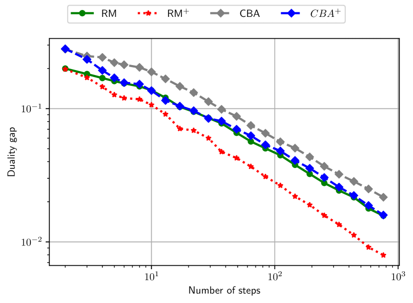
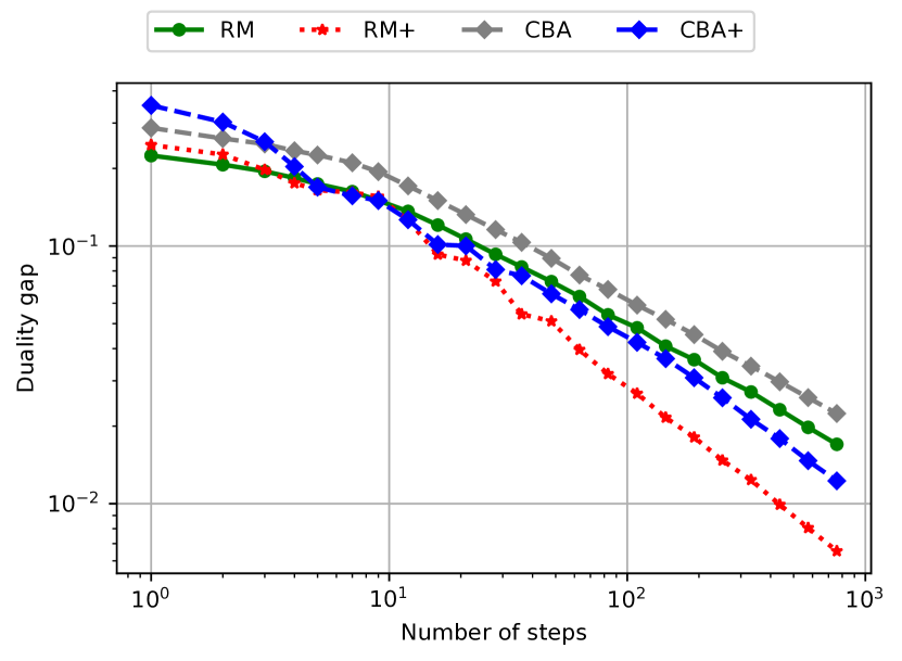
Refer to caption
(a) Without alternation nor linear averaging.
Refer to caption
(b) Without alternation but with linear averaging (only for RM+ and CBA+).
Refer to caption
(c) With alternation but no linear averaging.
Refer to caption
(d) With alternation and linear averaging.
Figure 6: Comparison of RM, RM+, CBA and CBA+ for 𝒳=Δ(n),𝒴=Δ(m)formulae-sequence𝒳Δ𝑛𝒴Δ𝑚\mathcal{X}=\Delta(n),\mathcal{Y}=\Delta(m) and random matrices, with and without alternations, and with and without linear averaging. We choose n,m=10𝑛𝑚10n,m=10 and AijU[0,1]similar-tosubscript𝐴𝑖𝑗𝑈01A_{ij}\sim U[0,1] over 707070 instances.
Refer to caption
(a) Without alternation nor linear averaging.
Refer to caption
(b) Without alternation but with linear averaging (only for RM+ and CBA+).
Refer to caption
(c) With alternation but no linear averaging.
Refer to caption
(d) With alternation and linear averaging.
Figure 7: Comparison of RM, RM+, CBA and CBA+ for 𝒳=Δ(n),𝒴=Δ(m)formulae-sequence𝒳Δ𝑛𝒴Δ𝑚\mathcal{X}=\Delta(n),\mathcal{Y}=\Delta(m) and random matrices, with and without alternations, and with and without linear averaging. We choose n,m=10𝑛𝑚10n,m=10 and AijN(0,1)similar-tosubscript𝐴𝑖𝑗𝑁01A_{ij}\sim N(0,1) over 707070 instances.

E.3 Additional numerical experiments for matrix games

We have seen in Appendix E.2 that RM+ and CBA+ with alternation and linear averaging are outperforming RM and CBA. In Figure 1(a), we have compared both RM+ and CBA+ with AdaFTRL (Orabona and Pál, 2015) and AdaHedge (De Rooij et al., 2014), two algorithms that also enjoy the desirable scale-free property, i.e., their sequences of decisions remain invariant when the losses are scaled by a constant factor. In the next figure, we provide additional comparisons of RM+, CBA+, AdaHedge and AdaFTRL when the coefficients of the matrix of payoff are normally distributed. We found that RM+ and CBA+ are both outperforming AdaHedge and AdaFTRL, a situation similar to the case of uniform payoffs (Figure 1(a).)
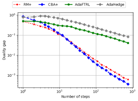
Refer to caption
Figure 8: Comparison of RM+, CBA+, AdaHedge and AdaFTRL for 𝒳=Δ(n),𝒴=Δ(m)formulae-sequence𝒳Δ𝑛𝒴Δ𝑚\mathcal{X}=\Delta(n),\mathcal{Y}=\Delta(m) and random matrices. We choose n,m=10𝑛𝑚10n,m=10 and AijN(0,1)similar-tosubscript𝐴𝑖𝑗𝑁01A_{ij}\sim N(0,1) over 707070 instances.

E.4 Additional numerical experiments for EFGs

In Section 4.1 , we have compared CBA+ (using alternation and linear averaging) and CFR+ on various EFGs instances. We present in Figure 9 additional simulations where CBA+ and CFR+ performs similarly. A description of the games can be found in Farina et al. (2021). On the y𝑦y-axis we show the duality gap of the current averaged decisions (𝒙¯T,𝒚¯T)subscript¯𝒙𝑇subscript¯𝒚𝑇(\bar{\bm{x}}_{T},\bar{\bm{y}}_{T}). On the x𝑥x-axis we show the number of iterations.
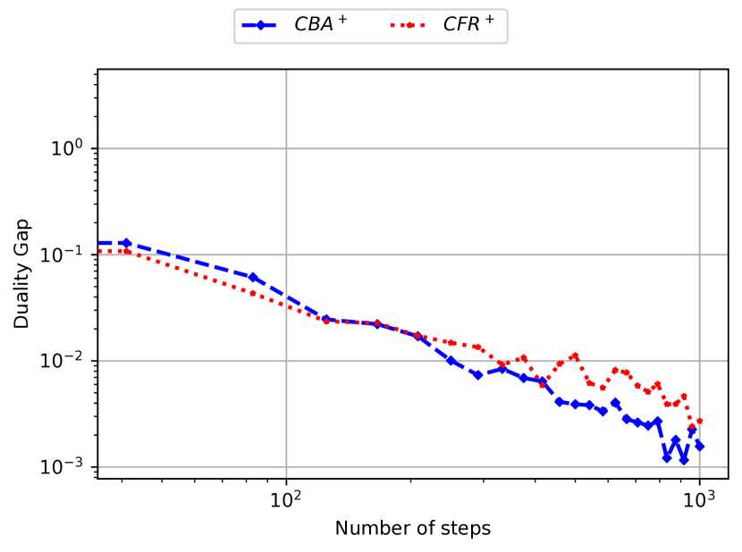
Refer to caption
(a) Search game, 4 turns.
Refer to caption
(b) Search game, 5 turns.
Refer to caption
(c) Leduc, 2 players, 3 ranks.
Refer to caption
(d) Leduc, 2 players, 6 faces.
Figure 9: Comparison of CBA+ and CFR+ for various Extensive-Form Games (EFG) instances.

Appendix F OMD, FTRL and optimistic variants

F.1 Algorithms

Let us fix some step size η>0𝜂0\eta>0. For solving our instances of distributionally robust optimization, we compare Algorithm CBA+ with the following four state-of-the-art algorithms:

  1. 1.

    Follow-The-Regularized-Leader (FTRL) (Abernethy et al., 2009; McMahan, 2011):

    𝒙t+1argmin𝒙𝒳τ=1t𝒇τ,𝒙+1η𝒙22.subscript𝒙𝑡1subscript𝒙𝒳superscriptsubscript𝜏1𝑡subscript𝒇𝜏𝒙1𝜂superscriptsubscriptnorm𝒙22\bm{x}_{t+1}\in\arg\min_{\bm{x}\in\mathcal{X}}\;\langle\sum_{\tau=1}^{t}\bm{f}_{\tau},\bm{x}\rangle+\dfrac{1}{\eta}\|\bm{x}\|_{2}^{2}. (FTRL)

    Optimistic FTRL (Rakhlin and Sridharan, 2013): given estimation 𝒎t+1superscript𝒎𝑡1\bm{m}^{t+1} of loss at period t+1𝑡1t+1, choose

    𝒙t+1argmin𝒙𝒳τ=1t𝒇τ+𝒎t+1,𝒙+1η𝒙22.subscript𝒙𝑡1subscript𝒙𝒳superscriptsubscript𝜏1𝑡subscript𝒇𝜏superscript𝒎𝑡1𝒙1𝜂superscriptsubscriptnorm𝒙22\bm{x}_{t+1}\in\arg\min_{\bm{x}\in\mathcal{X}}\;\langle\sum_{\tau=1}^{t}\bm{f}_{\tau}+\bm{m}^{t+1},\bm{x}\rangle+\dfrac{1}{\eta}\|\bm{x}\|_{2}^{2}. (O-FTRL)
  2. 2.

    Online Mirror Descent (OMD) (Nemirovski and Yudin, 1983; Beck and Teboulle, 2003):

    𝒙t+1min𝒙𝒳𝒇t,𝒙+1η𝒙𝒙t22.subscript𝒙𝑡1subscript𝒙𝒳subscript𝒇𝑡𝒙1𝜂superscriptsubscriptnorm𝒙subscript𝒙𝑡22\bm{x}_{t+1}\in\min_{\bm{x}\in\mathcal{X}}\langle\bm{f}_{t},\bm{x}\rangle+\dfrac{1}{\eta}\|\bm{x}-\bm{x}_{t}\|_{2}^{2}. (OMD)

    Optimistic OMD (Chiang et al., 2012): given estimation 𝒎t+1superscript𝒎𝑡1\bm{m}^{t+1} of loss at period t+1𝑡1t+1,

    𝒛t+1min𝒛𝒳𝒎t+1,𝒛+1η𝒛𝒙t22,subscript𝒛𝑡1subscript𝒛𝒳subscript𝒎𝑡1𝒛1𝜂superscriptsubscriptnorm𝒛subscript𝒙𝑡22\displaystyle\bm{z}_{t+1}\in\min_{\bm{z}\in\mathcal{X}}\langle\bm{m}_{t+1},\bm{z}\rangle+\dfrac{1}{\eta}\|\bm{z}-\bm{x}_{t}\|_{2}^{2}, (O-OMD)
    Observe the loss 𝒇t+1 related to 𝒛t+1,Observe the loss subscript𝒇𝑡1 related to subscript𝒛𝑡1\displaystyle\text{Observe the loss }\bm{f}_{t+1}\text{ related to }\bm{z}_{t+1},
    𝒙t+1min𝒙𝒳𝒇t+1,𝒙+1η𝒙𝒙t22.subscript𝒙𝑡1subscript𝒙𝒳subscript𝒇𝑡1𝒙1𝜂superscriptsubscriptnorm𝒙subscript𝒙𝑡22\displaystyle\bm{x}_{t+1}\in\min_{\bm{x}\in\mathcal{X}}\langle\bm{f}_{t+1},\bm{x}\rangle+\dfrac{1}{\eta}\|\bm{x}-\bm{x}_{t}\|_{2}^{2}.

Note that a priori these algorithms can be written more generally using Bregman divergence (e.g., Ben-Tal and Nemirovski (2001)). We choose to work with 2\|\cdot\|_{2} instead of Kullback-Leibler divergence as this 2subscript2\ell_{2}-setup is usually associated with faster empirical convergence rates (Chambolle and Pock, 2016; Gao et al., 2019). Additionally, following Chiang et al. (2012); Rakhlin and Sridharan (2013), we use the last observed loss as the predictor for the next loss, i.e., we set 𝒎t+1=𝒇tsuperscript𝒎𝑡1subscript𝒇𝑡\bm{m}^{t+1}=\bm{f}_{t}.

F.2 Implementations

When 𝒳𝒳\mathcal{X} is the simplex or a ball based on the 2subscript2\ell_{2}-distance and centered at 𝟎0\bm{0}, there is a closed-form solution to the proximal updates for FTRL, OMD, O-FTRL and O-OMD. However, it is not clear how to compute these proximal updates for different settings, e.g., when 𝒳𝒳\mathcal{X} is a subset of the simplex or an psubscript𝑝\ell_{p}-ball. We present the details of our implementation below. The results in the rest of this section are reminiscient to the novel tractable proximal setups presented in Grand-Clément and Kroer (2020a, b).

Computing the projection steps for min-player

For 𝒳={𝒙n|𝒙𝒙02ϵx}𝒳conditional-set𝒙superscript𝑛subscriptnorm𝒙subscript𝒙02subscriptitalic-ϵ𝑥\mathcal{X}=\{\bm{x}\in\mathbb{R}^{n}\;|\;\|\bm{x}-\bm{x}_{0}\|_{2}\leq\epsilon_{x}\}, 𝒄,𝒙n𝒄superscript𝒙superscript𝑛\bm{c},\bm{x}^{\prime}\in\mathbb{R}^{n} and a step size η>0𝜂0\eta>0, the prox-update becomes

min𝒙𝒙02ϵx𝒄,𝒙+12η𝒙𝒙22.subscriptsubscriptnorm𝒙subscript𝒙02subscriptitalic-ϵ𝑥𝒄𝒙12𝜂superscriptsubscriptnorm𝒙superscript𝒙22\min_{\|\bm{x}-\bm{x}_{0}\|_{2}\leq\epsilon_{x}}\langle\bm{c},\bm{x}\rangle+\dfrac{1}{2\eta}\|\bm{x}-\bm{x}^{\prime}\|_{2}^{2}. (31)

This is the same arg min as

min𝒙𝒙02ϵx𝒙(𝒙η𝒄)22.subscriptsubscriptnorm𝒙subscript𝒙02subscriptitalic-ϵ𝑥superscriptsubscriptnorm𝒙superscript𝒙𝜂𝒄22\min_{\|\bm{x}-\bm{x}_{0}\|_{2}\leq\epsilon_{x}}\|\bm{x}-(\bm{x}^{\prime}-\eta\bm{c})\|_{2}^{2}.

We can change 𝒙𝒙\bm{x} by 𝒛=(𝒙𝒙0)/ϵx𝒛𝒙subscript𝒙0subscriptitalic-ϵ𝑥\bm{z}=\left(\bm{x}-\bm{x}_{0}\right)/\epsilon_{x} to solve the equivalent program

min𝒛21𝒛1ϵx(𝒙η𝒄𝒙0)22.subscriptsubscriptnorm𝒛21superscriptsubscriptnorm𝒛1subscriptitalic-ϵ𝑥superscript𝒙𝜂𝒄subscript𝒙022\min_{\|\bm{z}\|_{2}\leq 1}\|\bm{z}-\dfrac{1}{\epsilon_{x}}\left(\bm{x}^{\prime}-\eta\bm{c}-\bm{x}_{0}\right)\|_{2}^{2}.

The solution to the above program is

𝒛=𝒙η𝒄𝒙0max{ϵx,𝒙η𝒄𝒙02}.𝒛superscript𝒙𝜂𝒄subscript𝒙0subscriptitalic-ϵ𝑥subscriptnormsuperscript𝒙𝜂𝒄subscript𝒙02\bm{z}=\dfrac{\bm{x}^{\prime}-\eta\bm{c}-\bm{x}_{0}}{\max\{\epsilon_{x},\|\bm{x}^{\prime}-\eta\bm{c}-\bm{x}_{0}\|_{2}\}}.

From 𝒙=𝒙0+ϵx𝒛𝒙subscript𝒙0subscriptitalic-ϵ𝑥𝒛\bm{x}=\bm{x}_{0}+\epsilon_{x}\bm{z} we obtain 𝒙superscript𝒙\bm{x}^{*} the solution to (31)

𝒙=𝒙0+ϵx𝒙η𝒄𝒙0max{ϵx,𝒙η𝒄𝒙02}.superscript𝒙subscript𝒙0subscriptitalic-ϵ𝑥superscript𝒙𝜂𝒄subscript𝒙0subscriptitalic-ϵ𝑥subscriptnormsuperscript𝒙𝜂𝒄subscript𝒙02\bm{x}^{*}=\bm{x}_{0}+\epsilon_{x}\dfrac{\bm{x}^{\prime}-\eta\bm{c}-\bm{x}_{0}}{\max\{\epsilon_{x},\|\bm{x}^{\prime}-\eta\bm{c}-\bm{x}_{0}\|_{2}\}}.

Computing the projection steps for max-player

For 𝒴={𝒚Δ(m)|𝒚𝒚02ϵy}𝒴conditional-set𝒚Δ𝑚subscriptnorm𝒚subscript𝒚02subscriptitalic-ϵ𝑦\mathcal{Y}=\{\bm{y}\in\Delta(m)\;|\;\|\bm{y}-\bm{y}_{0}\|_{2}\leq\epsilon_{y}\}, the proximal update of the max-player from a previous point 𝒚superscript𝒚\bm{y}^{\prime} and a step size of η>0𝜂0\eta>0 becomes

min𝒚𝒚02ϵy,𝒚Δ(m)𝒄,𝒚+12η𝒚𝒚22.subscriptformulae-sequencesubscriptnorm𝒚subscript𝒚02subscriptitalic-ϵ𝑦𝒚Δ𝑚𝒄𝒚12𝜂superscriptsubscriptnorm𝒚superscript𝒚22\min_{\|\bm{y}-\bm{y}_{0}\|_{2}\leq\epsilon_{y},\bm{y}\in\Delta(m)}\langle\bm{c},\bm{y}\rangle+\dfrac{1}{2\eta}\|\bm{y}-\bm{y}^{\prime}\|_{2}^{2}. (32)

If we dualize the 2subscript2\ell_{2} constraint with a Lagrangian multiplier μ0𝜇0\mu\geq 0 we obtain the relaxed problem q(μ)𝑞𝜇q(\mu) where

q(μ)=(1/2)ϵy2μ+min𝒚Δ(m)𝒄,𝒚+12η𝒚𝒚22+μ2𝒚𝒚022.𝑞𝜇12superscriptsubscriptitalic-ϵ𝑦2𝜇subscript𝒚Δ𝑚𝒄𝒚12𝜂superscriptsubscriptnorm𝒚superscript𝒚22𝜇2superscriptsubscriptnorm𝒚subscript𝒚022q(\mu)=-(1/2)\epsilon_{y}^{2}\mu+\min_{\bm{y}\in\Delta(m)}\langle\bm{c},\bm{y}\rangle+\dfrac{1}{2\eta}\|\bm{y}-\bm{y}^{\prime}\|_{2}^{2}+\dfrac{\mu}{2}\|\bm{y}-\bm{y}_{0}\|_{2}^{2}. (33)

Note that the argmin\arg\min in

min𝒚Δ(m)𝒄,𝒚+12η𝒚𝒚22+μ2𝒚𝒚022subscript𝒚Δ𝑚𝒄𝒚12𝜂superscriptsubscriptnorm𝒚superscript𝒚22𝜇2superscriptsubscriptnorm𝒚subscript𝒚022\min_{\bm{y}\in\Delta(m)}\langle\bm{c},\bm{y}\rangle+\dfrac{1}{2\eta}\|\bm{y}-\bm{y}^{\prime}\|_{2}^{2}+\dfrac{\mu}{2}\|\bm{y}-\bm{y}_{0}\|_{2}^{2}

is the same argmin\arg\min as in

min𝒚Δ(m)𝒚ηημ+1(1η𝒚+μ𝒚0𝒄)22.subscript𝒚Δ𝑚superscriptsubscriptnorm𝒚𝜂𝜂𝜇11𝜂superscript𝒚𝜇subscript𝒚0𝒄22\min_{\bm{y}\in\Delta(m)}\|\bm{y}-\dfrac{\eta}{\eta\mu+1}\left(\dfrac{1}{\eta}\bm{y}^{\prime}+\mu\bm{y}_{0}-\bm{c}\right)\|_{2}^{2}. (34)

Note that (34) is an orthogonal projection onto the simplex. Therefore, it can be solved efficiently (Duchi et al., 2008). We call 𝒚(μ)𝒚𝜇\bm{y}(\mu) an optimal solution of (34). Then q(μ)𝑞𝜇q(\mu) can be rewritten

q(μ)=(1/2)ϵy2μ+𝒄,𝒚(μ)+12η𝒚(μ)𝒚22+μ2𝒚(μ)𝒚022.𝑞𝜇12superscriptsubscriptitalic-ϵ𝑦2𝜇𝒄𝒚𝜇12𝜂superscriptsubscriptnorm𝒚𝜇superscript𝒚22𝜇2superscriptsubscriptnorm𝒚𝜇subscript𝒚022q(\mu)=-(1/2)\epsilon_{y}^{2}\mu+\langle\bm{c},\bm{y}(\mu)\rangle+\dfrac{1}{2\eta}\|\bm{y}(\mu)-\bm{y}^{\prime}\|_{2}^{2}+\dfrac{\mu}{2}\|\bm{y}(\mu)-\bm{y}_{0}\|_{2}^{2}.

We can therefore binary search q(μ)𝑞𝜇q(\mu) as in the previous expression. An upper bound μ¯¯𝜇\bar{\mu} for μsuperscript𝜇\mu^{*} can be computed as follows. Note that

q(μ)(1/2)ϵy2μ+𝒄,𝒚0+12η𝒚0𝒚22.𝑞𝜇12superscriptsubscriptitalic-ϵ𝑦2𝜇𝒄subscript𝒚012𝜂superscriptsubscriptnormsubscript𝒚0superscript𝒚22q(\mu)\leq-(1/2)\epsilon_{y}^{2}\mu+\langle\bm{c},\bm{y}_{0}\rangle+\dfrac{1}{2\eta}\|\bm{y}_{0}-\bm{y}^{\prime}\|_{2}^{2}.

Since μq(μ)maps-to𝜇𝑞𝜇\mu\mapsto q(\mu) is concave we can choose μ¯¯𝜇\bar{\mu} such that q(μ)q(0)𝑞𝜇𝑞0q(\mu)\leq q(0). Using the previous inequality this yields

μ¯=2ϵy2(𝒄,𝒚0+12η𝒚0𝒚22q(0)).¯𝜇2superscriptsubscriptitalic-ϵ𝑦2𝒄subscript𝒚012𝜂superscriptsubscriptnormsubscript𝒚0superscript𝒚22𝑞0\bar{\mu}=\frac{2}{\epsilon_{y}^{2}}\left(\langle\bm{c},\bm{y}_{0}\rangle+\dfrac{1}{2\eta}\|\bm{y}_{0}-\bm{y}^{\prime}\|_{2}^{2}-q(0)\right).

We choose a precision of ϵ=0.001italic-ϵ0.001\epsilon=0.001 in our simulations. Note that these binary searches make OMD, FTRL, O-FTRL and O-OMD slower than CBA+ in terms of running times, since the updates in CBA+ only requires to compute the projection π𝒞(𝒖)subscript𝜋𝒞𝒖\pi_{\mathcal{C}}(\bm{u}), and we have shown in Proposition D.4 and Appendix D.2 how to compute this in O(n)𝑂𝑛O(n) when 𝒳𝒳\mathcal{X} is an 2subscript2\ell_{2} ball 𝒳={𝒙Δ(n)|𝒙𝒙02ϵx}𝒳conditional-set𝒙Δ𝑛subscriptnorm𝒙subscript𝒙02subscriptitalic-ϵ𝑥\mathcal{X}=\{\bm{x}\in\Delta(n)\;|\;\|\bm{x}-\bm{x}_{0}\|_{2}\leq\epsilon_{x}\}.

Computing the theoretical step sizes

We now give details about the choice of choice of theoretical step sizes. In theory (e.g., Ben-Tal and Nemirovski (2001)), for a player with decision set 𝒳𝒳\mathcal{X}, we can choose η𝗍𝗁=2Ω/LTsubscript𝜂𝗍𝗁2Ω𝐿𝑇\eta_{\sf th}=\sqrt{2}\Omega/L\sqrt{T} with Ω=max𝒙,𝒙𝒳𝒙𝒙2Ωsubscript𝒙superscript𝒙𝒳subscriptnorm𝒙superscript𝒙2\Omega=\max_{\bm{x},\bm{x}^{\prime}\in\mathcal{X}}\|\bm{x}-\bm{x}^{\prime}\|_{2}, and L𝐿L an upper bound on the norm of any observed loss 𝒇tsubscript𝒇𝑡\bm{f}_{t}: 𝒇t2L,t1formulae-sequencesubscriptnormsubscript𝒇𝑡2𝐿for-all𝑡1\|\bm{f}_{t}\|_{2}\leq L,\forall\;t\geq 1. Note that this requires to know 1) the number of steps T𝑇T, and 2) the upper bound L𝐿L on the norm of any observed loss 𝒇tsubscript𝒇𝑡\bm{f}_{t}, before the losses are generated. We now show how to compute Lxsubscript𝐿𝑥L_{x} and Lysubscript𝐿𝑦L_{y} (for the x𝑥x-player and the y𝑦y-player) for an instance of the distributionally robust optimization problem (5).

  1. 1.

    For the y𝑦y-player, the loss𝒇tsubscript𝒇𝑡\bm{f}_{t} is 𝒇t=(i(𝒙t))i[1,m]subscript𝒇𝑡subscriptsubscript𝑖subscript𝒙𝑡𝑖1𝑚\bm{f}_{t}=\left(\ell_{i}(\bm{x}_{t})\right)_{i\in[1,m]}, with i(𝒙)=log(1+exp(bi𝒂i𝒙))subscript𝑖𝒙1subscript𝑏𝑖subscriptsuperscript𝒂top𝑖𝒙\ell_{i}(\bm{x})=\log(1+\exp(-b_{i}\bm{a}^{\top}_{i}\bm{x})). For each i[1,m]𝑖1𝑚i\in[1,m] we have |i|log(1+exp(|bi|R𝒂i2))subscript𝑖1subscript𝑏𝑖𝑅subscriptnormsubscript𝒂𝑖2|\ell_{i}|\leq\log(1+\exp(|b_{i}|R\|\bm{a}_{i}\|_{2})) so that

    Ly=i=1mlog(1+exp(|bi|R𝒂i2))2.L_{y}=\sqrt{\sum_{i=1}^{m}\log(1+\exp(|b_{i}|R\|\bm{a}_{i}\|_{2}))^{2}}.
  2. 2.

    For the x𝑥x-player we have 𝒇t=𝑨t𝒚tsubscript𝒇𝑡superscript𝑨𝑡subscript𝒚𝑡\bm{f}_{t}=\bm{A}^{t}\bm{y}_{t}, where 𝑨tsuperscript𝑨𝑡\bm{A}^{t} is the matrix of subgradients of 𝒙F(𝒙,𝒚t)maps-to𝒙𝐹𝒙subscript𝒚𝑡\bm{x}\mapsto F(\bm{x},\bm{y}_{t}) at 𝒙tsubscript𝒙𝑡\bm{x}_{t}:

    Aijt=11+exp(bi𝒂i𝒙t)biai,j,(i,j){1,,m}×{1,,n}.formulae-sequencesubscriptsuperscript𝐴𝑡𝑖𝑗11subscript𝑏𝑖superscriptsubscript𝒂𝑖topsubscript𝒙𝑡subscript𝑏𝑖subscript𝑎𝑖𝑗for-all𝑖𝑗1𝑚1𝑛A^{t}_{ij}=\dfrac{-1}{1+\exp(b_{i}\bm{a}_{i}^{\top}\bm{x}_{t})}b_{i}a_{i,j},\forall\;(i,j)\in\{1,...,m\}\times\{1,...,n\}.

    Therefore, 𝒇t2𝑨t2𝒚t2𝑨t2subscriptnormsubscript𝒇𝑡2subscriptnormsuperscript𝑨𝑡2subscriptnormsubscript𝒚𝑡2subscriptnormsuperscript𝑨𝑡2\|\bm{f}_{t}\|_{2}\leq\|\bm{A}^{t}\|_{2}\|\bm{y}_{t}\|_{2}\leq\|\bm{A}^{t}\|_{2}, because 𝒚Δ(m)𝒚Δ𝑚\bm{y}\in\Delta(m). Now we have 𝑨t2𝑨tF=i,j|Aijt|2subscriptnormsuperscript𝑨𝑡2subscriptnormsuperscript𝑨𝑡𝐹subscript𝑖𝑗superscriptsuperscriptsubscript𝐴𝑖𝑗𝑡2\|\bm{A}^{t}\|_{2}\leq\|\bm{A}^{t}\|_{F}=\sqrt{\sum_{i,j}|A_{ij}^{t}|^{2}}. From |Aijt||biai,j|subscriptsuperscript𝐴𝑡𝑖𝑗subscript𝑏𝑖subscript𝑎𝑖𝑗|A^{t}_{ij}|\leq|b_{i}a_{i,j}| we use

    Lx=i,j|biai,j|2.subscript𝐿𝑥subscript𝑖𝑗superscriptsubscript𝑏𝑖subscript𝑎𝑖𝑗2L_{x}=\sqrt{\sum_{i,j}|b_{i}a_{i,j}|^{2}}.

Appendix G Additional details and numerical experiments for distributionally robust optimization

We compare CBA+ with alternation and linear averaging, OMD,FTRL,O-OMD and O-OMD for various step sizes η𝜂\eta where η=αη𝗍𝗁𝜂𝛼subscript𝜂𝗍𝗁\eta=\alpha\eta_{\sf th} for α{1,100,1,000,10,000}𝛼1100100010000\alpha\in\{1,100,1,000,10,000\}, on additional synthetic and real data sets. We also add a comparison with adaptive step sizes.

Data sets

We present here the characteristics of the data sets that we use in our DRO simulations. All data sets can be downloaded from the libsvm classification libraries333https://www.csie.ntu.edu.tw/similar-to\simcjlin/libsvmtools/datasets/

  • Adult data set: two classes, m=1,605𝑚1605m=1,605 samples with n=123𝑛123n=123 features.

  • Australian data set: two classes, m=690𝑚690m=690 samples with n=14𝑛14n=14 features.

  • Madelon data set: two classes, m=2,000𝑚2000m=2,000 samples with n=500𝑛500n=500 features.

  • Splice data set: two classes, m=1,000𝑚1000m=1,000 samples with n=60𝑛60n=60 features.

Additional experiments with fixed step sizes

In this section we present additional numerical experiments for solving distributionally robust optimization instances in Figure 10. We use a synthetic data set, where we sample the features aijsubscript𝑎𝑖𝑗a_{ij} as uniform random variables in [0,1]01[0,1]. We also present results for the adult and the australian data sets from libsvm. We vary the aggressiveness of the step sizes η=αη𝗍𝗁𝜂𝛼subscript𝜂𝗍𝗁\eta=\alpha\eta_{\sf th} by multiplying the theoretical step sizes η𝗍𝗁subscript𝜂𝗍𝗁\eta_{\sf th} by a multiplicative step factor α𝛼\alpha. The empirical setting is the same as in Section 4. We note that our algorithm still outperforms or performs on par with the classical approaches after 102superscript10210^{2} iterations, without requiring a single choice of parameter.
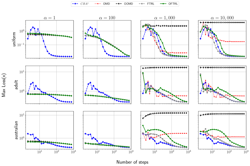
Refer to caption
Figure 10: Comparisons of the performances of CBA+ with alternation and linear averaging, OMD,FTRL,O-OMD and O-FTRL on synthetic (with uniform distribution) and real data sets (adult and australian). We use fixed step sizes η=αη𝗍𝗁𝜂𝛼subscript𝜂𝗍𝗁\eta=\alpha\eta_{\sf th}, where η𝗍𝗁subscript𝜂𝗍𝗁\eta_{\sf th} is the theoretical step size that guarantees convergence.

Additional experiments with adaptive step sizes

We present our additional results with adaptive step sizes in Figure 11. Given 𝒗tsubscript𝒗𝑡\bm{v}_{t} the payoff observed by the player at period t𝑡t, and following Orabona (2019), we choose the step sizes (ηt)t1subscriptsubscript𝜂𝑡𝑡1\left(\eta_{t}\right)_{t\geq 1} as

ηt=1/τ=1t𝒗τ22.subscript𝜂𝑡1superscriptsubscript𝜏1𝑡superscriptsubscriptnormsubscript𝒗𝜏22\eta_{t}=1/\sqrt{\sum_{\tau=1}^{t}\|\bm{v}_{\tau}\|_{2}^{2}}. (35)

We note that CBA+ still outperforms, or performs on par, with the state-of-the-art approaches.
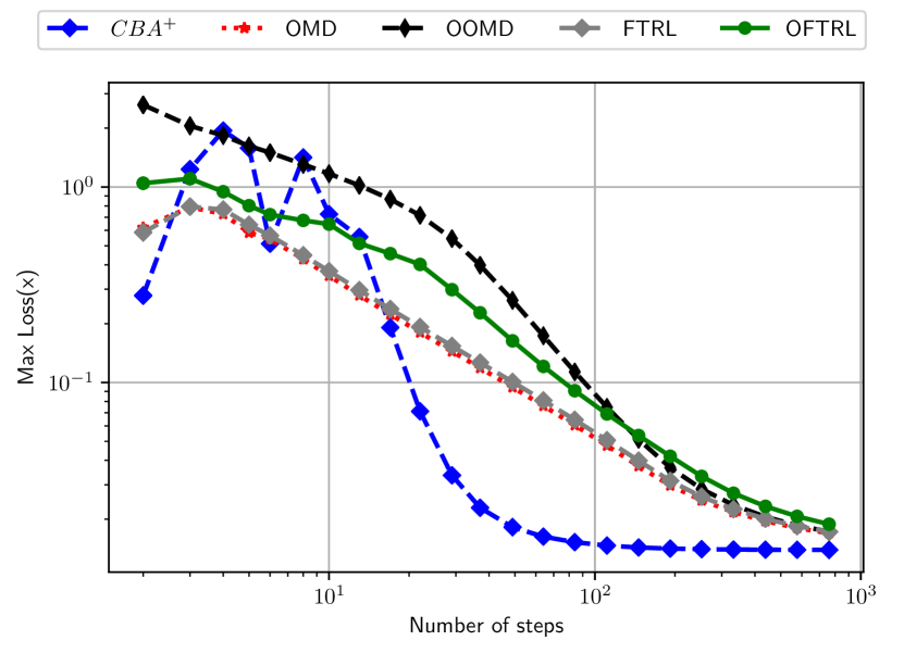
Refer to caption
(a) Uniform.
Refer to caption
(b) Adult
Refer to caption
(c) Australian
Figure 11: Comparisons of the performances of CBA+ with alternation and linear averaging, OMD,FTRL,O-OMD and O-FTRL on synthetic (with uniform distribution) and real data sets (adult and australian). For the non-parameter free algorithms, we use the adaptive step sizes as in (35).