Simulation of Conditioned Semimartingales on Riemannian Manifolds

\nameMathias HΓΈjgaard Jensen and Stefan Sommer Contact: Stefan Sommer, sommer@di.ku.dk Department of Computer Science, University of Copenhagen, Denmark
Abstract

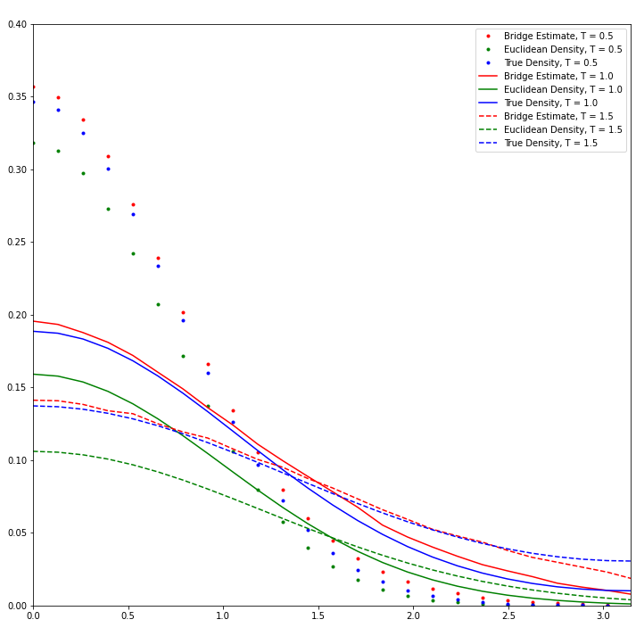
We present a scheme for simulating conditioned semimartingales taking values in Riemannian manifolds. Extending the guided bridge proposal approach used for simulating Euclidean bridges, the scheme replaces the drift of the conditioned process with an approximation in terms of a scaled radial vector field. This handles the fact that transition densities are generally intractable on geometric spaces. We prove the validity of the scheme by a change of measure argument, and we show how the resulting guided processes can be used in importance sampling and for approximating the density of the unconditioned process. The scheme is used for numerically simulating bridges on two- and three-dimensional manifolds, for approximating otherwise intractable transition densities, and for estimating the diffusion mean of sampled geometric data.

keywords:
bridge simulation, conditioned diffusions, diffusion mean, geometric statistics, Riemannian manifolds

1 Introduction

Techniques for simulating Euclidean diffusion bridge processes, bridge sampling, have been studied in several cases over the last two decades, for instance [9, 10, 29, 36]. Delyon & Hu [10] introduced a scheme to simulate conditioned diffusions using a stochastic differential equation (SDE) that can be directly simulated and is absolutely continuous with respect to the desired distribution. The SDE interchanged a drift term depending on the possibly intractable transition density with a drift arising from a Brownian bridge going from aπ‘Ža to b𝑏b in time T𝑇T for a,bβˆˆβ„dπ‘Žπ‘superscriptℝ𝑑a,b\in\mathbb{R}^{d}.

We here propose a scheme for simulating conditioned semimartingales on Riemannian manifolds. This generalizes the result of Delyon and Hu [10] to the setting of smooth connected Riemannian manifolds. We prove analytically that the result holds on a variety of manifolds, including the space of symmetric positive definite matrices considered by Bui et al. [8]. More precisely, we show that by adding a drift term to the semimartingale, the manifold equivalent to the drift term introduced in [10] to approximate the gradient of the log-transition density, we obtain a process that converges to the desired endpoint. The process is absolutely continuous with respect to the targeted diffusion bridge distribution.

Bridge sampling is an essential part of likelihood and Bayesian inference for discretely observed stochastic processes. For example, bridge sampling finds applications in geometric statistics, medical imaging, and shape analysis. Recent papers have introduced algorithms to simulate stochastic bridges on specific manifolds [7, 8, 3, 20, 31], which indicate the necessity for bridge sampling algorithms on general Riemannian manifolds. In particular, the ability to estimate the transition density of a stochastic process enables likelihood-based and Bayesian approaches to geometric statistics.

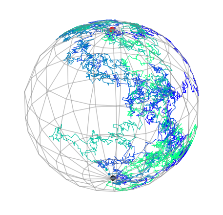
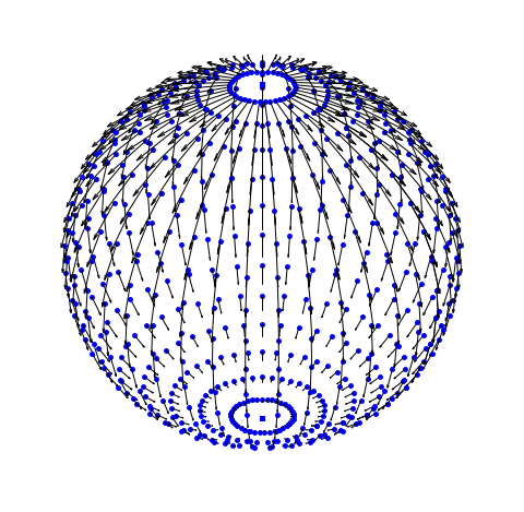
Figure 1(a) shows sample paths generated by the sampling scheme set up to approximate a conditioned Brownian motion on the sphere π•Š2superscriptπ•Š2\mathbb{S}^{2} starting at the north pole and conditioned to hit the south pole at T=1𝑇1T=1. The scaled squared radial vector field, βˆ‡d​(β‹…,v)22​(Tβˆ’t)βˆ‡π‘‘superscript⋅𝑣22𝑇𝑑\tfrac{\nabla d(\cdot,v)^{2}}{2(T-t)} Figure 1(b) acts as the guiding term forcing the process towards the target v𝑣v.

Refer to caption
(a) Four simulated paths of a diffusion bridge process from the north pole (red point) to the south pole (black point)
Refer to caption
(b) Gradient vector field of the squared distance function on the 222-sphere centered at the south pole.
Figure 1: Realizations of the bridge simulation scheme in a case where the target point is in the cut locus of the starting point, and the guiding vector field that approximates the score.
Refer to caption
βˆ‡d​(Xt,v)22βˆ‡π‘‘superscriptsubscript𝑋𝑑𝑣22\frac{\nabla d(X_{t},v)^{2}}{2}

Cut⁑(v)Cut𝑣\operatorname{Cut}(v)

XT=vsubscript𝑋𝑇𝑣X_{T}=v

Xtsubscript𝑋𝑑X_{t}

X0=xsubscript𝑋0π‘₯X_{0}=x

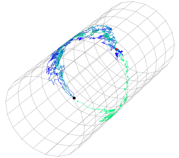
(a) Illustration of a sample path of a radial bridge, Xtsubscript𝑋𝑑X_{t}, from starting point xπ‘₯x to target v𝑣v with corresponding guiding drift indicated by arrows. The drift discontinuously changes sign when crossing the cut locus of the target (vertical line).
Refer to caption
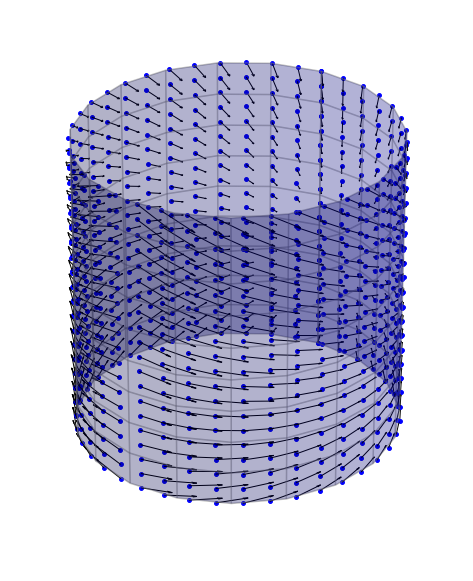
(b) Radial vector field on the cylinder, Xtsubscript𝑋𝑑X_{t}, centered at the target v𝑣v.
Figure 2: Illustration of the effect of the cut locus on the radial bridge process. The guiding drift term, indicated by the tangent vectors along the sample path in (a) and the radial vector field (b) discontinuosly changes directions when crossing discontinuosly the cut locus.

1.1 Guided proposals

Doob’s hβ„Žh-transform is a classical way to show that the SDE for the conditioned process has a drift term that depends on the gradient of the logarithmic transition density, the score βˆ‡xlog⁑p​(t,x,v)subscriptβˆ‡π‘₯𝑝𝑑π‘₯𝑣\nabla_{x}\log p(t,x,v). Due to the generally intractable transition density, various methods to simulate conditioned processes have been introduced (e.g., [9, 10, 29, 36]).

Delyon & Hu [10] presented an algorithm to simulate the distribution of certain types of diffusions in ℝdsuperscriptℝ𝑑\mathbb{R}^{d} conditioned to hit a terminal point, at some fixed time T>0𝑇0T>0. Their main idea was to substitute the drift βˆ‡xlog⁑p​(t,x,v)subscriptβˆ‡π‘₯𝑝𝑑π‘₯𝑣\nabla_{x}\log p(t,x,v), which depends on the transition density, with the drift term appearing in the SDE for the generalized Brownian bridge. More precisely, they showed that the law of the process

d​Xt=b​(t,Xt)​d​t+σ​(t,Xt)​d​Wt,X0=a,formulae-sequence𝑑subscript𝑋𝑑𝑏𝑑subscriptπ‘‹π‘‘π‘‘π‘‘πœŽπ‘‘subscript𝑋𝑑𝑑subscriptπ‘Šπ‘‘subscript𝑋0π‘ŽdX_{t}=b(t,X_{t})dt+\sigma(t,X_{t})dW_{t},\qquad X_{0}=a,

conditioned on XT=vsubscript𝑋𝑇𝑣X_{T}=v is absolutely continuous with respect to the law of the process

d​Yt=b​(t,Yt)​d​tβˆ’Ytβˆ’vTβˆ’t+σ​(t,Yt)​d​Wt,Y0=aformulae-sequence𝑑subscriptπ‘Œπ‘‘π‘π‘‘subscriptπ‘Œπ‘‘π‘‘π‘‘subscriptπ‘Œπ‘‘π‘£π‘‡π‘‘πœŽπ‘‘subscriptπ‘Œπ‘‘π‘‘subscriptπ‘Šπ‘‘subscriptπ‘Œ0π‘ŽdY_{t}=b(t,Y_{t})dt-\frac{Y_{t}-v}{T-t}+\sigma(t,Y_{t})dW_{t},\qquad Y_{0}=a (1)

under suitable conditions on b𝑏b and ΟƒπœŽ\sigma. Moreover, the conditional expectation given XT=vsubscript𝑋𝑇𝑣X_{T}=v satisfies

𝔼​[f​(X)|XT=v]=C​𝔼​[f​(Y)​φT],𝔼delimited-[]conditional𝑓𝑋subscript𝑋𝑇𝑣𝐢𝔼delimited-[]π‘“π‘Œsubscriptπœ‘π‘‡\mathbb{E}\left[f(X)|X_{T}=v\right]=C\mathbb{E}\left[f(Y)\varphi_{T}\right], (2)

for a constant C>0𝐢0C>0, where Ο†Tsubscriptπœ‘π‘‡\varphi_{T} denotes the likelihood ratio. We present a result that generalizes the SDE in (1) and essentially also equation (2) to Riemannian manifolds, with an explicit expression for the likelihood ratio Ο†Tsubscriptπœ‘π‘‡\varphi_{T}.

Switching from vector space to Riemannian manifolds, curvature removes the closed form solution of the Brownian bridge drift. Inspired by Delyon and Hu’s construction and the notion of Fermi bridges [34, 35], we instead propose to use the gradient βˆ‡xd​(β‹…,v)2/2subscriptβˆ‡π‘₯𝑑superscript⋅𝑣22\nabla_{x}d(\cdot,v)^{2}/2 in the drift term in a non-Euclidean generalization of (1). However, the existence of a non-trivial cut locus implies that this radial vector field is not continuous. Moreover, the tβ†’0→𝑑0t\to 0 convergence of the term to the gradient of the log-density is more intricate than the Euclidean situation. As shown by Malliavin, Stroock [25], and Turetsky [32],

limtβ†’0tβ€‹βˆ‡xmlog⁑pℳ​(t,x,v)=βˆ’βˆ‡xmd​(x,v)2/2,for all ​mβ‰₯0,formulae-sequencesubscript→𝑑0𝑑subscriptsuperscriptβˆ‡π‘šπ‘₯subscript𝑝ℳ𝑑π‘₯𝑣subscriptsuperscriptβˆ‡π‘šπ‘₯𝑑superscriptπ‘₯𝑣22for allΒ π‘š0\lim_{t\to 0}t\nabla^{m}_{x}\log p_{\mathcal{M}}(t,x,v)=-\nabla^{m}_{x}d(x,v)^{2}/2,\qquad\text{for all }m\geq 0, (3)

uniformly on compact subsets of β„³\Cut⁑(v)\β„³Cut𝑣\mathcal{M}\backslash\operatorname{Cut}(v), where βˆ‡msuperscriptβˆ‡π‘š\nabla^{m} is the mπ‘šmth covariant derivative and pβ„³subscript𝑝ℳp_{\mathcal{M}} the heat kernel or the transition density of a Brownian motion on a manifold β„³β„³\mathcal{M}. The behaviour of the right hand side of (3), for m=1π‘š1m=1, is illustrated in Figure 2. The cut locus adds extra difficulty because the squared distance is not differentiable on the cut locus, and the convergence in (3) is only uniform away from the cut locus.

1.2 Bridge sampling: Parameter, density, and metric estimation

Bridge processes are useful in a range of statistical and applied mathematical problems. We here list a few examples: Bridge sampling is essential for building data augmentation algorithms [36]. Treating sample points as if coming from incomplete observations, bridge sampling algorithms provides a better understanding of the underlying distribution, thereby offering a method for parameter estimation. Delyon and Hu [10] presents a rather specific example of parameter estimation using bridge sampling. Furthermore, bridge sampling techniques can be applied to estimate normalizing constants (see, e.g., [15]).

Statistical models based on diffusion processes find applications in geometric statistics, see, e.g. [27]. In particular, bridge sampling on manifolds yields estimates of the diffusion mean [16, 17]. The diffusion mean relies on the transition density of a Brownian motion and is a generalization of the FrΓ©chet mean, defined as the argument that minimizes the average of distances. In this case, bridge sampling approximates the transition density or data likelihood. We demonstrate in the numerical examples how bridge sampling can be used to approximate the transition density and to find diffusion means.

Estimation of transition densities by bridge sampling find uses in shape analysis [1, 2, 31], e.g. for estimating the underlying Riemannian metric given shape observations.

1.3 Outline

In SectionΒ 2, we review relevant existing work on manifold bridge processes and the frame bundle theory used to describe stochastic integration on manifolds. SectionΒ 3 describes the Radon-Nikodym derivative related to the change of measure and a Cameron-Martin-Girsanov change of measure result. In SectionΒ 4, we present our two main results that generalize [10, Theorem 5] to manifold-valued semimartingales. SectionΒ 5 is devoted to the radial process. We apply Barden and Le’s result [22, Theorem 3] to the radial process and show the almost sure convergence of our guided process. We go on to rigorously prove the two propositions in SectionΒ 6, before ending with numerical examples in SectionΒ 7. We visualize the result of the simulation scheme on two- and three-dimensional manifolds, and we use the approach to approximate the heat kernel on different 2-dimensional manifolds. Furthermore, we provide examples of how iterative bridge sampling can be used to estimate diffusion means.

1.4 Notation and conventions

Throughout the paper, we use the following notation and make the listed assumptions:

  • β€’

    (Ξ©,β„±,(β„±t)tβ‰₯0,β„™)Ξ©β„±subscriptsubscriptℱ𝑑𝑑0β„™(\Omega,\mathcal{F},(\mathcal{F}_{t})_{t\geq 0},\mathbb{P}) is a complete filtered probability space satisfying the usual conditions, i.e., the filtration (β„±t)tβ‰₯0subscriptsubscriptℱ𝑑𝑑0(\mathcal{F}_{t})_{t\geq 0} is complete and right-continuous.

  • β€’

    β„³β„³\mathcal{M} is a d𝑑d-dimensional smooth manifold.

  • β€’

    Wtsubscriptπ‘Šπ‘‘W_{t} a d𝑑d-dimensional Euclidean Brownian motion.

  • β€’

    Ztsubscript𝑍𝑑Z_{t} an d𝑑d-dimensional Euclidean semimartingale, a solution to the SDE d​Zt=b​(t,Zt)​d​t+σ​(t,Zt)​d​Wt𝑑subscript𝑍𝑑𝑏𝑑subscriptπ‘π‘‘π‘‘π‘‘πœŽπ‘‘subscript𝑍𝑑𝑑subscriptπ‘Šπ‘‘dZ_{t}=b(t,Z_{t})dt+\sigma(t,Z_{t})dW_{t}, for suitably integrable b𝑏b and ΟƒπœŽ\sigma.

  • β€’

    Utsubscriptπ‘ˆπ‘‘U_{t} a horizontal semimartingale in the frame bundle ℱ​ℳℱℳ\mathcal{FM}.

  • β€’

    Xtsubscript𝑋𝑑X_{t} a β„³β„³\mathcal{M}-valued semimartingale defined as the projection Xt:=π​(Ut)assignsubscriptπ‘‹π‘‘πœ‹subscriptπ‘ˆπ‘‘X_{t}:=\pi(U_{t}).

  • β€’

    rv​(Xt):=d​(Xt,v)assignsubscriptπ‘Ÿπ‘£subscript𝑋𝑑𝑑subscript𝑋𝑑𝑣r_{v}(X_{t}):=d(X_{t},v) is the Riemannian distance between Xtsubscript𝑋𝑑X_{t} and vβˆˆβ„³π‘£β„³v\in\mathcal{M}.

  • β€’

    Both the diffusion field Οƒt​(z):=σ​(t,z)assignsubscriptπœŽπ‘‘π‘§πœŽπ‘‘π‘§\sigma_{t}(z):=\sigma(t,z) and its inverse Οƒtβˆ’1​(z)subscriptsuperscript𝜎1𝑑𝑧\sigma^{-1}_{t}(z) are bounded and differentiable .

  • β€’

    The bracket process [Z]delimited-[]𝑍[Z] is absolutely continuous as a random measure on [0,∞)0[0,\infty).

  • β€’

    The set {t:Xt∈Cut⁑(v)}conditional-set𝑑subscript𝑋𝑑Cut𝑣\{t\colon X_{t}\in\operatorname{Cut}(v)\} is a Lebesgue null-set.

  • β€’

    All SDEs admits strong solutions.

We will use ~~absent\tilde{\,} to denote lifts of functions on M𝑀M to fiber bundles, i.e., with projection Ο€πœ‹\pi, f~:=fβˆ˜Ο€assign~π‘“π‘“πœ‹\tilde{f}:=f\circ\pi. As the distance function d​(β‹…,y)𝑑⋅𝑦d(\cdot,y) is non-differentiable on the cut locus, we take βˆ‡xd​(x,y)subscriptβˆ‡π‘₯𝑑π‘₯𝑦\nabla_{x}d(x,y) to be the usual gradient away from cut locus and define it to be zero at the cut locus. We will repeatedly use the Einstein summation convention.

2 Background

2.1 Manifold valued processes

We review the theory of frame bundles and manifold-valued diffusion processes. In particular, we describe the main concepts of differential geometry, which are needed to define the Eells-Elworthy-Malliavin construction of manifold-valued stochastic processes through horizontal lifts. Two common references for stochastic calculus on manifolds are Emery [14] and Hsu [18].

2.1.1 Riemannian geometry

The frame bundle ℱ​ℳℱℳ\mathcal{FM} of a d𝑑d-dimensional smooth manifold is a d2+dsuperscript𝑑2𝑑d^{2}+d dimensional manifold, where each point uβˆˆβ„±β€‹β„³π‘’β„±β„³u\in\mathcal{FM} correspond to a point xβˆˆβ„³π‘₯β„³x\in\mathcal{M} together with an ordered basis (frame) of the tangent space Tx​ℳsubscript𝑇π‘₯β„³T_{x}\mathcal{M}. It is convenient to think of u𝑒u as a linear bijection u:ℝdβ†’Tπ​(u)​ℳ:𝑒→superscriptℝ𝑑subscriptπ‘‡πœ‹π‘’β„³u\colon\mathbb{R}^{d}\rightarrow T_{\pi(u)}\mathcal{M}, where Ο€:ℱ​ℳ→ℳ:πœ‹β†’β„±β„³β„³\pi\colon\mathcal{FM}\rightarrow\mathcal{M} denotes the canonical projection. In this sense we obtain an ordered basis (u​(e1),…,u​(ed))𝑒subscript𝑒1…𝑒subscript𝑒𝑑(u(e_{1}),...,u(e_{d})) of Tπ​(u)​ℳsubscriptπ‘‡πœ‹π‘’β„³T_{\pi(u)}\mathcal{M} from the canonical basis (e1,…,ed)subscript𝑒1…subscript𝑒𝑑(e_{1},...,e_{d}) of ℝdsuperscriptℝ𝑑\mathbb{R}^{d}. A connection in ℱ​ℳℱℳ\mathcal{FM} is a smooth choice of subspaces β„‹uβ€‹β„±β€‹β„³βŠ†Tu​ℱ​ℳsubscriptℋ𝑒ℱℳsubscript𝑇𝑒ℱℳ\mathcal{H}_{u}\mathcal{FM}\subseteq T_{u}\mathcal{FM}, for each uβˆˆβ„±β€‹β„³π‘’β„±β„³u\in\mathcal{FM}, such that the tangent space at uβˆˆβ„±β€‹β„³π‘’β„±β„³u\in\mathcal{FM} splits into Tu​ℱ​ℳ=𝒱uβ€‹β„±β€‹β„³βŠ•β„‹u​ℱ​ℳsubscript𝑇𝑒ℱℳdirect-sumsubscript𝒱𝑒ℱℳsubscriptℋ𝑒ℱℳT_{u}\mathcal{FM}=\mathcal{V}_{u}\mathcal{FM}\oplus\mathcal{H}_{u}\mathcal{FM}, where 𝒱u​ℱ​ℳsubscript𝒱𝑒ℱℳ\mathcal{V}_{u}\mathcal{FM} denotes the tangent vectors that are tangent to the fibers. The space β„‹u​ℱ​ℳsubscriptℋ𝑒ℱℳ\mathcal{H}_{u}\mathcal{FM} is called the horizontal tangent space. If we endow β„³β„³\mathcal{M} with a Riemannian structure, that is, a smoothly varying inner product on the tangent spaces, the set of frames can be restricted to orthonormal frames, i.e., the map u𝑒u being a linear isometry. The resulting subbundle is denoted the orthonormal frame bundle, π’ͺ​ℳπ’ͺβ„³\mathcal{OM}. We will throughout primarily work with π’ͺ​ℳπ’ͺβ„³\mathcal{OM}. There is a one-to-one correspondence between the horizontal tangent space at u𝑒u and the tangent space at π​(u)πœ‹π‘’\pi(u). This correspondence is described through the restriction of the pushforward map Ο€βˆ—|β„‹u​π’ͺ​ℳ:Tu​π’ͺ​ℳ→Tπ​(u)​ℳ:evaluated-atsubscriptπœ‹subscriptℋ𝑒π’ͺβ„³β†’subscript𝑇𝑒π’ͺβ„³subscriptπ‘‡πœ‹π‘’β„³\pi_{*}|_{\mathcal{H}_{u}\mathcal{OM}}\colon T_{u}\mathcal{OM}\rightarrow T_{\pi(u)}\mathcal{M}. Furthermore, on the horizontal part of the frame bundle, there exists a set of fundamental horizontal vector fields, H1,…,Hdsubscript𝐻1…subscript𝐻𝑑H_{1},...,H_{d}, defined by Hi​(u)=hu​(u​(ei))subscript𝐻𝑖𝑒subscriptβ„Žπ‘’π‘’subscript𝑒𝑖H_{i}(u)=h_{u}\left(u(e_{i})\right), where hu=(Ο€βˆ—|β„‹u​π’ͺ​ℳ)βˆ’1subscriptβ„Žπ‘’superscriptevaluated-atsubscriptπœ‹subscriptℋ𝑒π’ͺβ„³1h_{u}=\left(\pi_{*}|_{\mathcal{H}_{u}\mathcal{OM}}\right)^{-1} is the horizontal lift.

It is sometimes convenient to linearize the manifold in the following sense. Let E:ℝdβ†’Tp​ℳ:𝐸→superscriptℝ𝑑subscript𝑇𝑝ℳE\colon\mathbb{R}^{d}\rightarrow T_{p}\mathcal{M} be an isometric isomorphism from d𝑑d-dimensional Euclidean space to the tangent space at pβˆˆβ„³π‘β„³p\in\mathcal{M} and let Expp:Tp​ℳ→ℳ:subscriptExp𝑝→subscript𝑇𝑝ℳℳ\operatorname{Exp}_{p}\colon T_{p}\mathcal{M}\rightarrow\mathcal{M} denote the exponential map at p𝑝p. Define Ο•:D→ℝd:italic-ϕ→𝐷superscriptℝ𝑑\phi\colon D\rightarrow\mathbb{R}^{d} by Ο•:=Eβˆ’1∘Exppβˆ’1assignitalic-Ο•superscript𝐸1superscriptsubscriptExp𝑝1\phi:=E^{-1}\circ\operatorname{Exp}_{p}^{-1}, where DβŠ†β„³π·β„³D\subseteq\mathcal{M} is the largest subset such that Logp:=Exppβˆ’1assignsubscriptLog𝑝superscriptsubscriptExp𝑝1\operatorname{Log}_{p}:=\operatorname{Exp}_{p}^{-1} is well-defined, then the pair (D,Ο•)𝐷italic-Ο•(D,\phi) is a normal neighborhood centered at pβˆˆβ„³π‘β„³p\in\mathcal{M}.

2.1.2 Horizontal semimartingales - stochastic development

When the starting frame U0subscriptπ‘ˆ0U_{0} is fixed, there exists a one-to-one correspondence between Euclidean-, horizontal-, and manifold-valued curves. If ztsubscript𝑧𝑑z_{t} is an ℝdsuperscriptℝ𝑑\mathbb{R}^{d} curve with derivative d​zt𝑑subscript𝑧𝑑dz_{t}, then Hd​zt​(ut)=hut​(ut​(ei))​d​zti=Hi​(ut)​d​ztisubscript𝐻𝑑subscript𝑧𝑑subscript𝑒𝑑subscriptβ„Žsubscript𝑒𝑑subscript𝑒𝑑subscript𝑒𝑖𝑑superscriptsubscript𝑧𝑑𝑖subscript𝐻𝑖subscript𝑒𝑑𝑑superscriptsubscript𝑧𝑑𝑖H_{dz_{t}}(u_{t})=h_{u_{t}}(u_{t}(e_{i}))dz_{t}^{i}=H_{i}(u_{t})dz_{t}^{i}. The construction is called horizontal development and extends to include semimartingales.

If Z𝑍Z is a continuous Euclidean-valued semimartingale, i.e., a process which decomposes into a sum of a local martingale and an adapted process of locally bounded variation, the horizontal vector fields give rise to an SDE on the frame bundle, driven by the Stratonovich SDE,

d​Ut=Hi​(Ut)∘d​Zti,U0=uβˆˆβ„±β€‹β„³,formulae-sequence𝑑subscriptπ‘ˆπ‘‘subscript𝐻𝑖subscriptπ‘ˆπ‘‘π‘‘subscriptsuperscript𝑍𝑖𝑑subscriptπ‘ˆ0𝑒ℱℳdU_{t}=H_{i}(U_{t})\circ dZ^{i}_{t},\qquad U_{0}=u\in\mathcal{FM}, (4)

where Uπ‘ˆU is a horizontal semimartingale on π’ͺ​ℳπ’ͺβ„³\mathcal{OM}. The canonical projection, X:=π​(U)assignπ‘‹πœ‹π‘ˆX:=\pi(U), defines a process on β„³β„³\mathcal{M}. The process Uπ‘ˆU is called the stochastic development of Z𝑍Z in π’ͺ​ℳπ’ͺβ„³\mathcal{OM} and X𝑋X the stochastic development of Z𝑍Z in β„³β„³\mathcal{M}. Similarly, Z𝑍Z is called the anti-development of X𝑋X and Uπ‘ˆU. This way of constructing stochastic processes on manifolds is contributed to Eells, Elworthy, and Malliavin, and is often referred to as the Eells-Elworthy-Malliavin construction. In colloquial terms, the construction is called "rolling without slipping." The intuition behind this terminology originates from rolling a ball along a path drawn with wet ink on a piece of paper. For a detailed description of this construction, one may consult [18].

Define h~usubscript~β„Žπ‘’\tilde{h}_{u} as the solution to the stochastic development equation (4), i.e., h~u​(Zt)=Utsubscript~β„Žπ‘’subscript𝑍𝑑subscriptπ‘ˆπ‘‘\tilde{h}_{u}(Z_{t})=U_{t}. We call this map the stochastic development map. Similarly, we define the stochastic anti-development map as h~uβˆ’1​(Ut)=Ztsuperscriptsubscript~β„Žπ‘’1subscriptπ‘ˆπ‘‘subscript𝑍𝑑\tilde{h}_{u}^{-1}(U_{t})=Z_{t}.

2.1.3 Geometric ItΓ΄ formula

The fundamental theorem of stochastic calculus is Itô’s formula. The formula generalizes to manifold-valued semimartingales. If X𝑋X is a continuous manifold-valued semimartingale, Uπ‘ˆU its horizontal lift, and Z𝑍Z its anti-development, then for any smooth function f∈Cβˆžβ€‹(β„³)𝑓superscript𝐢ℳf\in C^{\infty}(\mathcal{M}) the geometric ItΓ΄ formula can be expressed as

d​f​(Xt)=Ut​(ei)​f​(Xt)​d​Zti+12​Ut​(ej)​Ut​(ek)​f​(Xt)​d​[Zj,Zk]t.𝑑𝑓subscript𝑋𝑑subscriptπ‘ˆπ‘‘subscript𝑒𝑖𝑓subscript𝑋𝑑𝑑subscriptsuperscript𝑍𝑖𝑑12subscriptπ‘ˆπ‘‘subscript𝑒𝑗subscriptπ‘ˆπ‘‘subscriptπ‘’π‘˜π‘“subscript𝑋𝑑𝑑subscriptsuperscript𝑍𝑗superscriptπ‘π‘˜π‘‘df(X_{t})=U_{t}(e_{i})f(X_{t})dZ^{i}_{t}+\tfrac{1}{2}U_{t}(e_{j})U_{t}(e_{k})f(X_{t})d[Z^{j},Z^{k}]_{t}.

The formula can equivalently be expressed in terms of the gradient and Hessian as

d​f​(Xt)=βŸ¨βˆ‡f​(Xt),Ut​d​Zt⟩Xt+12​HessXt⁑f​(Ut,Ut)​d​[Z]t,𝑑𝑓subscript𝑋𝑑subscriptβˆ‡π‘“subscript𝑋𝑑subscriptπ‘ˆπ‘‘π‘‘subscript𝑍𝑑subscript𝑋𝑑12subscriptHesssubscript𝑋𝑑𝑓subscriptπ‘ˆπ‘‘subscriptπ‘ˆπ‘‘π‘‘subscriptdelimited-[]𝑍𝑑df(X_{t})=\left\langle\nabla f(X_{t}),U_{t}dZ_{t}\right\rangle_{X_{t}}+\tfrac{1}{2}\operatorname{Hess}_{X_{t}}f(U_{t},U_{t})d[Z]_{t},

where βŸ¨β‹…,β‹…βŸ©xsubscriptβ‹…β‹…π‘₯\langle\cdot,\cdot\rangle_{x} denotes the Riemannian inner product on Tx​ℳsubscript𝑇π‘₯β„³T_{x}\mathcal{M}. We simply write βŸ¨β‹…,β‹…βŸ©β‹…β‹…\langle\cdot,\cdot\rangle when the subscript is clear from the context.

2.1.4 Riemannian Brownian bridges

Brownian bridges on manifolds also have an SDE representation. Whenever the semimartingale Z𝑍Z is a Brownian motion, the resulting process X𝑋X on β„³β„³\mathcal{M} (resp. Uπ‘ˆU on the horizontal part of π’ͺ​ℳπ’ͺβ„³\mathcal{OM}) is a Brownian motion. With p​(t,x,v)𝑝𝑑π‘₯𝑣p(t,x,v) denoting the transition density of the β„³β„³\mathcal{M}-valued Brownian motion and p~​(t,u,v)=p​(t,π​(u),v)~π‘π‘‘π‘’π‘£π‘π‘‘πœ‹π‘’π‘£\tilde{p}(t,u,v)=p(t,\pi(u),v) its lift to π’ͺ​ℳπ’ͺβ„³\mathcal{OM}, the corresponding Brownian bridge is the solution of the SDE

d​Ut=Hi​(Ut)∘(d​Bti+(Utβˆ’1​(Ο€βˆ—β€‹βˆ‡u|u=UtHlog⁑p~​(t,u,v)))i​d​t),U0=u0,formulae-sequence𝑑subscriptπ‘ˆπ‘‘subscript𝐻𝑖subscriptπ‘ˆπ‘‘π‘‘subscriptsuperscript𝐡𝑖𝑑superscriptsuperscriptsubscriptπ‘ˆπ‘‘1subscriptπœ‹superscriptsubscriptβˆ‡evaluated-at𝑒𝑒subscriptπ‘ˆπ‘‘π»~𝑝𝑑𝑒𝑣𝑖𝑑𝑑subscriptπ‘ˆ0subscript𝑒0dU_{t}=H_{i}(U_{t})\circ\left(dB^{i}_{t}+\left(U_{t}^{-1}\left(\pi_{*}\nabla_{u|_{u=U_{t}}}^{H}\log\tilde{p}(t,u,v)\right)\right)^{i}dt\right),\qquad U_{0}=u_{0}, (5)

where βˆ‡Hf~={H1​f~,…,Hd​f~}superscriptβˆ‡π»~𝑓subscript𝐻1~𝑓…subscript𝐻𝑑~𝑓\nabla^{H}\tilde{f}=\{H_{1}\tilde{f},\dots,H_{d}\tilde{f}\} is the horizontal gradient. As was the case in the Euclidean setting, the SDE includes the Brownian motion’s transition density. However, unlike the Euclidean case for Brownian motion, the transition density is generally not computable in closed-form.

Writing the transition density for the Brownian motion as p​(t,x,v)=pt​(x,v)𝑝𝑑π‘₯𝑣subscript𝑝𝑑π‘₯𝑣p(t,x,v)=p_{t}(x,v), a natural representation of the Brownian bridge is as a time-inhomogeneous Markov process with an infinitesimal generator

12​Δℳ+βˆ‡log⁑pTβˆ’t​(β‹…,v),12subscriptΞ”β„³βˆ‡subscript𝑝𝑇𝑑⋅𝑣\tfrac{1}{2}\Delta_{\mathcal{M}}+\nabla\log p_{T-t}(\cdot,v),

where Ξ”β„³subscriptΞ”β„³\Delta_{\mathcal{M}} is the generalized Laplacian (Laplace-Beltrami) operator on β„³β„³\mathcal{M}. We will drop the β„³β„³\mathcal{M} in the sequel whenever referring to the Laplace-Beltrami operator.

2.1.5 Related constructions

As the Brownian motion’s transition density is only known in a closed-form on few manifolds, other types of bridge processes have been considered (see e.g. [19]). A semi-classical Brownian bridge on a Riemannian, also known as Brownian Riemannian bridge, is a time inhomogeneous strong Markov process with infinitesimal generator

12​Δ+βˆ‡log⁑kTβˆ’t​(β‹…,v),12Ξ”βˆ‡subscriptπ‘˜π‘‡π‘‘β‹…π‘£\tfrac{1}{2}\Delta+\nabla\log k_{T-t}(\cdot,v),

where ktsubscriptπ‘˜π‘‘k_{t} is the function defined by

kt​(x,v):=(2​π​t)βˆ’n/2​eβˆ’r2​(x,v)2​t​Jβˆ’1/2​(x),assignsubscriptπ‘˜π‘‘π‘₯𝑣superscript2πœ‹π‘‘π‘›2superscript𝑒superscriptπ‘Ÿ2π‘₯𝑣2𝑑superscript𝐽12π‘₯k_{t}(x,v):=(2\pi t)^{-n/2}e^{-\frac{r^{2}(x,v)}{2t}}J^{-1/2}(x),

and J​(x)=|detDExpvβˆ’1⁑(x)​Expv|𝐽π‘₯subscript𝐷superscriptsubscriptExp𝑣1π‘₯subscriptExp𝑣J(x)=|\det D_{\operatorname{Exp}_{v}^{-1}(x)}\operatorname{Exp}_{v}| is the Jacobian determinant of the exponential map at v𝑣v (see any of [11, 12, 13] for more details on semi-classical bridges). This description typically relies on the existence of a pole, i.e. a point in β„³β„³\mathcal{M} where the exponential map maps diffeomorphically to β„³β„³\mathcal{M}. The assumption avoids the nuissance of the cut locus. The radial part of the semi-classical bridge has the distribution of a Euclidean valued Brownian bridge.

A generalization beyond the cut locus of the heat kernel formula described by Elworthy and Truman [12] is due to Thompson [34]. Let N𝑁N be a closed embedded submanifold on β„³β„³\mathcal{M} and define the distance function to N𝑁N by rN​(β‹…):=d​(β‹…,N)assignsubscriptπ‘Ÿπ‘β‹…π‘‘β‹…π‘r_{N}(\cdot):=d(\cdot,N), then introduce the diffusion on β„³β„³\mathcal{M} with time-dependent infinitesimal generator

12β€‹Ξ”β„³βˆ’βˆ‡rN22​(Tβˆ’t)=12β€‹Ξ”β„³βˆ’rNTβˆ’tβ€‹βˆ‚βˆ‚rN,12subscriptΞ”β„³βˆ‡subscriptsuperscriptπ‘Ÿ2𝑁2𝑇𝑑12subscriptΞ”β„³subscriptπ‘Ÿπ‘π‘‡π‘‘subscriptπ‘Ÿπ‘\frac{1}{2}\Delta_{\mathcal{M}}-\frac{\nabla r^{2}_{N}}{2(T-t)}\quad=\quad\frac{1}{2}\Delta_{\mathcal{M}}-\frac{r_{N}}{T-t}\frac{\partial}{\partial r_{N}},

where βˆ‚βˆ‚rNsubscriptπ‘Ÿπ‘\tfrac{\partial}{\partial r_{N}} denotes differentiation in the radial direction and ΔΔ\Delta denotes the Laplace-Beltrami operator. This diffusion process is called a Fermi bridge (see [34, 35]). More generally, [23] defined generalised Brownian bridge processes, between x0subscriptπ‘₯0x_{0} and xT=vsubscriptπ‘₯𝑇𝑣x_{T}=v with terminal time T𝑇T, as a Markov process (xt)tβ‰₯0subscriptsubscriptπ‘₯𝑑𝑑0(x_{t})_{t\geq 0} with infinitesimal generator

12β€‹Ξ”β„³βˆ’f​(t)β€‹βˆ‡rv22,12subscriptΞ”β„³π‘“π‘‘βˆ‡subscriptsuperscriptπ‘Ÿ2𝑣2\tfrac{1}{2}\Delta_{\mathcal{M}}-f(t)\nabla\tfrac{r^{2}_{v}}{2},

where f𝑓f is a suitably smooth real valued function defined on [0,1)01[0,1) satisfying limt↑Tf​(t)=∞subscript↑𝑑𝑇𝑓𝑑\lim_{t\uparrow T}f(t)=\infty and limt↑Txt=xTsubscript↑𝑑𝑇subscriptπ‘₯𝑑subscriptπ‘₯𝑇\lim_{t\uparrow T}x_{t}=x_{T} almost surely. We also refer the reader to [24] for a description of hypoelliptic bridges on manifolds.

3 A Girsanov change of measure

Intractable transition densities complicate exact simulation of the conditioned processes: For example, it is not possible to directly simulate from (5) if p~~𝑝\tilde{p} cannot be computed to get the score and the corresponding drift. Various methods exist to approximate these processes [6, 5, 9, 10, 29, 36]. Common for all these method is that they rely on a change of measure argument and that the changed measure respects the original measure, in the sense of absolute continuity.

In this section, we recall a Cameron-Martin-Girsanov result for manifold valued processes, see [11], that we will need later on. We assume throughout that Xt=π​(Ut)subscriptπ‘‹π‘‘πœ‹subscriptπ‘ˆπ‘‘X_{t}=\pi(U_{t}) is non-explosive. This is for example the case if β„³β„³\mathcal{M} is compact. Let d​Mt=Οƒt​(Zt)​d​Wt𝑑subscript𝑀𝑑subscriptπœŽπ‘‘subscript𝑍𝑑𝑑subscriptπ‘Šπ‘‘dM_{t}=\sigma_{t}(Z_{t})dW_{t} be the martingale part of Z𝑍Z, where we have assumed that ΟƒπœŽ\sigma is invertible. Define the local martingale Ltsubscript𝐿𝑑L_{t} by the equation

Lt:=βˆ’βˆ«0tβŸ¨βˆ‡u|u=UsHr~v2​(u)2​(Tβˆ’s),U​(ei)βŸ©β€‹π‘‘Msi.assignsubscript𝐿𝑑superscriptsubscript0𝑑subscriptsuperscriptβˆ‡π»evaluated-at𝑒𝑒subscriptπ‘ˆπ‘ subscriptsuperscript~π‘Ÿ2𝑣𝑒2π‘‡π‘ π‘ˆsubscript𝑒𝑖differential-dsuperscriptsubscript𝑀𝑠𝑖L_{t}:=-\int_{0}^{t}\left\langle\frac{\nabla^{H}_{u|_{u=U_{s}}}\tilde{r}^{2}_{v}(u)}{2(T-s)},U(e_{i})\right\rangle dM_{s}^{i}.

Using that Uπ‘ˆU is an isometry, the local martingale is identical to the process

Lt:=βˆ’βˆ«0tβŸ¨Οƒsβˆ’1​(h~uβˆ’1​(Us))​Usβˆ’1​(βˆ‡u|u=UsHr~v2​(u)2​(Tβˆ’s)),ejβŸ©β€‹π‘‘Wsj.assignsubscript𝐿𝑑superscriptsubscript0𝑑subscriptsuperscript𝜎1𝑠superscriptsubscript~β„Žπ‘’1subscriptπ‘ˆπ‘ superscriptsubscriptπ‘ˆπ‘ 1subscriptsuperscriptβˆ‡π»evaluated-at𝑒𝑒subscriptπ‘ˆπ‘ subscriptsuperscript~π‘Ÿ2𝑣𝑒2𝑇𝑠subscript𝑒𝑗differential-dsuperscriptsubscriptπ‘Šπ‘ π‘—L_{t}:=-\int_{0}^{t}\left\langle\sigma^{-1}_{s}(\tilde{h}_{u}^{-1}(U_{s}))U_{s}^{-1}\left(\frac{\nabla^{H}_{u|_{u=U_{s}}}\tilde{r}^{2}_{v}(u)}{2(T-s)}\right),e_{j}\right\rangle dW_{s}^{j}.

The corresponding Radon-Nikodym derivative is given by

Dt=exp⁑[Ltβˆ’12β€‹βˆ«0tβˆ₯Οƒsβˆ’1​(h~uβˆ’1​(Us))​Usβˆ’1​(βˆ‡u|u=UsHr~v2​(u)2​(Tβˆ’s))βˆ₯2​𝑑s].subscript𝐷𝑑subscript𝐿𝑑12superscriptsubscript0𝑑superscriptdelimited-βˆ₯βˆ₯subscriptsuperscript𝜎1𝑠superscriptsubscript~β„Žπ‘’1subscriptπ‘ˆπ‘ subscriptsuperscriptπ‘ˆ1𝑠subscriptsuperscriptβˆ‡π»evaluated-at𝑒𝑒subscriptπ‘ˆπ‘ subscriptsuperscript~π‘Ÿ2𝑣𝑒2𝑇𝑠2differential-d𝑠D_{t}=\exp\bigg{[}L_{t}-\frac{1}{2}\int_{0}^{t}\bigg{\lVert}\sigma^{-1}_{s}(\tilde{h}_{u}^{-1}(U_{s}))U^{-1}_{s}\left(\frac{\nabla^{H}_{u|_{u=U_{s}}}\tilde{r}^{2}_{v}(u)}{2(T-s)}\right)\bigg{\rVert}^{2}ds\bigg{]}. (6)

The Novikov condition ensures that the measure β„štsubscriptβ„šπ‘‘\mathbb{Q}_{t}, defined as dβ€‹β„št=Dt​d​ℙ𝑑subscriptβ„šπ‘‘subscript𝐷𝑑𝑑ℙd\mathbb{Q}_{t}=D_{t}d\mathbb{P}, is equivalent to the measure β„™β„™\mathbb{P} on the time interval [0,T)0𝑇[0,T). As a consequence of Girsanov’s theorem, we have that the β„™tsubscriptℙ𝑑\mathbb{P}_{t}-Brownian motion, Wtsubscriptπ‘Šπ‘‘W_{t}, satisfies the equation

d​Wt=d​W^tβˆ’Οƒtβˆ’1​(h~uβˆ’1​(Ut))​Utβˆ’1​(βˆ‡u|u=UsHr~v2​(u)2​(Tβˆ’t))​d​t,𝑑subscriptπ‘Šπ‘‘π‘‘subscript^π‘Šπ‘‘subscriptsuperscript𝜎1𝑑superscriptsubscript~β„Žπ‘’1subscriptπ‘ˆπ‘‘superscriptsubscriptπ‘ˆπ‘‘1subscriptsuperscriptβˆ‡π»evaluated-at𝑒𝑒subscriptπ‘ˆπ‘ subscriptsuperscript~π‘Ÿ2𝑣𝑒2𝑇𝑑𝑑𝑑dW_{t}=d\hat{W}_{t}-\sigma^{-1}_{t}(\tilde{h}_{u}^{-1}(U_{t}))U_{t}^{-1}\left(\frac{\nabla^{H}_{u|_{u=U_{s}}}\tilde{r}^{2}_{v}(u)}{2(T-t)}\right)dt,

and we have that W^tsubscript^π‘Šπ‘‘\hat{W}_{t} is a β„štsubscriptβ„šπ‘‘\mathbb{Q}_{t}-Brownian motion. Plugging the expression for Wtsubscriptπ‘Šπ‘‘W_{t} into equation (4) yields the SDE

d​Ut=Hi​(Ut)∘(d​Ztiβˆ’(Utβˆ’1​(βˆ‡Hr~v2​(Ut)2​(Tβˆ’t)))i​d​t).𝑑subscriptπ‘ˆπ‘‘subscript𝐻𝑖subscriptπ‘ˆπ‘‘π‘‘subscriptsuperscript𝑍𝑖𝑑superscriptsuperscriptsubscriptπ‘ˆπ‘‘1superscriptβˆ‡π»subscriptsuperscript~π‘Ÿ2𝑣subscriptπ‘ˆπ‘‘2𝑇𝑑𝑖𝑑𝑑dU_{t}=H_{i}(U_{t})\circ\biggl{(}dZ^{i}_{t}-\left(U_{t}^{-1}\left(\frac{\nabla^{H}\tilde{r}^{2}_{v}(U_{t})}{2(T-t)}\right)\right)^{i}dt\biggr{)}. (7)

We will consider solutions to this SDE and its projection to β„³β„³\mathcal{M} throughout the paper. We term the solution of (7) the radial bridge process. The added drift can equivalently we written βˆ’Hi​r~v2​(Ut)2​(Tβˆ’t)subscript𝐻𝑖subscriptsuperscript~π‘Ÿ2𝑣subscriptπ‘ˆπ‘‘2𝑇𝑑-\frac{H_{i}\tilde{r}^{2}_{v}(U_{t})}{2(T-t)} because (Utβˆ’1​(Ο€βˆ—β€‹βˆ‡Hr~v2​(Ut)))i=βŸ¨βˆ‡rv2​(Xt),Ut​(ei)⟩=Hi​r~v2​(Ut)superscriptsuperscriptsubscriptπ‘ˆπ‘‘1subscriptπœ‹superscriptβˆ‡π»superscriptsubscript~π‘Ÿπ‘£2subscriptπ‘ˆπ‘‘π‘–βˆ‡superscriptsubscriptπ‘Ÿπ‘£2subscript𝑋𝑑subscriptπ‘ˆπ‘‘subscript𝑒𝑖subscript𝐻𝑖superscriptsubscript~π‘Ÿπ‘£2subscriptπ‘ˆπ‘‘\left(U_{t}^{-1}\left(\pi_{*}\nabla^{H}\tilde{r}_{v}^{2}(U_{t})\right)\right)^{i}=\left\langle\nabla r_{v}^{2}(X_{t}),U_{t}(e_{i})\right\rangle=H_{i}\tilde{r}_{v}^{2}(U_{t}).

Example 3.1.

Consider the case where the driving semimartingale is a standard Brownian motion. The Radon-Nikodym derivative (6) simplifies to

Dt:=exp⁑[βˆ’βˆ«0trN​(Xs)Tβˆ’sβ€‹βŸ¨βˆ‚βˆ‚rN,Us​d​BsβŸ©βˆ’12β€‹βˆ«0trN2​(Xs)(Tβˆ’s)2​𝑑s],assignsubscript𝐷𝑑superscriptsubscript0𝑑subscriptπ‘Ÿπ‘subscript𝑋𝑠𝑇𝑠subscriptπ‘Ÿπ‘subscriptπ‘ˆπ‘ π‘‘subscript𝐡𝑠12superscriptsubscript0𝑑superscriptsubscriptπ‘Ÿπ‘2subscript𝑋𝑠superscript𝑇𝑠2differential-d𝑠D_{t}:=\exp\bigg{[}-\int_{0}^{t}\frac{r_{N}(X_{s})}{T-s}\bigg{\langle}\frac{\partial}{\partial r_{N}},U_{s}dB_{s}\bigg{\rangle}-\frac{1}{2}\int_{0}^{t}\frac{r_{N}^{2}(X_{s})}{(T-s)^{2}}ds\bigg{]}, (8)

almost surely, since the norm of the gradient of the radial process is constantly one away from the cut locus and its starting point, Cut⁑(x0)βˆͺ{x0}Cutsubscriptπ‘₯0subscriptπ‘₯0\operatorname{Cut}(x_{0})\cup\{x_{0}\}, and since this set is polar for X𝑋X. In particular, as mentioned in [35], the integral

∫0tβŸ¨βˆ‚βˆ‚rN,Us​d​Bs⟩=Ξ²tsuperscriptsubscript0𝑑subscriptπ‘Ÿπ‘subscriptπ‘ˆπ‘ π‘‘subscript𝐡𝑠subscript𝛽𝑑\int_{0}^{t}\bigg{\langle}\frac{\partial}{\partial r_{N}},U_{s}dB_{s}\bigg{\rangle}=\beta_{t}

is a one-dimensional standard Brownian motion, which follows from Levy’s characterization theorem of Brownian motions and that Uπ‘ˆU consists of isometries.

4 Bridge simulation on manifolds

This section initiates horizontal semimartingales from Euclidean-valued semimartingales and describes the guided semimartingales considered in this paper. Throughout, we assume that Z=(Z1,Z2,…,Zd)𝑍superscript𝑍1superscript𝑍2…superscript𝑍𝑑Z=(Z^{1},Z^{2},...,Z^{d}) is a Euclidean-valued semimartingale given by

d​Ztk=ak​(t,Zt)​d​t+Οƒmk​(t,Zt)​d​Wtm,𝑑superscriptsubscriptπ‘π‘‘π‘˜superscriptπ‘Žπ‘˜π‘‘subscript𝑍𝑑𝑑𝑑superscriptsubscriptπœŽπ‘šπ‘˜π‘‘subscript𝑍𝑑𝑑superscriptsubscriptπ‘Šπ‘‘π‘šdZ_{t}^{k}=a^{k}(t,Z_{t})dt+\sigma_{m}^{k}(t,Z_{t})dW_{t}^{m}, (9)

where Wπ‘ŠW is a Euclidean-Brownian motion and aπ‘Ža and ΟƒπœŽ\sigma are suitably integrable maps. Horizontal semimartingales are then obtained as solutions to (4) which evidentally happens if and only if, for all smooth functions f~~𝑓\tilde{f} on π’ͺ​ℳπ’ͺβ„³\mathcal{OM}, it holds that

d​f~​(Ut)=Hi​f~​(Ut)∘d​Zti.𝑑~𝑓subscriptπ‘ˆπ‘‘subscript𝐻𝑖~𝑓subscriptπ‘ˆπ‘‘π‘‘subscriptsuperscript𝑍𝑖𝑑d\tilde{f}(U_{t})=H_{i}\tilde{f}(U_{t})\circ dZ^{i}_{t}.

By the ItΓ΄-Stratonovich conversion, we obtain the corresponding ItΓ΄ equation

d​f~​(Ut)=β„’~u​f~​(Ut)​d​t+Οƒmk​(t,h~uβˆ’1​(Ut))​Hk​f~​(Ut)​d​Wtm,𝑑~𝑓subscriptπ‘ˆπ‘‘subscript~ℒ𝑒~𝑓subscriptπ‘ˆπ‘‘π‘‘π‘‘superscriptsubscriptπœŽπ‘šπ‘˜π‘‘superscriptsubscript~β„Žπ‘’1subscriptπ‘ˆπ‘‘subscriptπ»π‘˜~𝑓subscriptπ‘ˆπ‘‘π‘‘subscriptsuperscriptπ‘Šπ‘šπ‘‘d\tilde{f}(U_{t})=\tilde{\mathcal{L}}_{u}\tilde{f}(U_{t})dt+\sigma_{m}^{k}(t,\tilde{h}_{u}^{-1}(U_{t}))H_{k}\tilde{f}(U_{t})dW^{m}_{t},

where β„’~usubscript~ℒ𝑒\tilde{\mathcal{L}}_{u} is an operator in π’ͺ​ℳπ’ͺβ„³\mathcal{OM} defined by

β„’~u​f~​(Ut):=ak​(t,h~uβˆ’1​(Ut))​Hk​f~​(Ut)+12​Ci​j​(t,h~uβˆ’1​(Ut))​Hi​Hj​f~​(Ut),assignsubscript~ℒ𝑒~𝑓subscriptπ‘ˆπ‘‘superscriptπ‘Žπ‘˜π‘‘superscriptsubscript~β„Žπ‘’1subscriptπ‘ˆπ‘‘subscriptπ»π‘˜~𝑓subscriptπ‘ˆπ‘‘12superscript𝐢𝑖𝑗𝑑superscriptsubscript~β„Žπ‘’1subscriptπ‘ˆπ‘‘subscript𝐻𝑖subscript𝐻𝑗~𝑓subscriptπ‘ˆπ‘‘\tilde{\mathcal{L}}_{u}\tilde{f}(U_{t}):=a^{k}(t,\tilde{h}_{u}^{-1}(U_{t}))H_{k}\tilde{f}(U_{t})+\tfrac{1}{2}C^{ij}(t,\tilde{h}_{u}^{-1}(U_{t}))H_{i}H_{j}\tilde{f}(U_{t}), (10)

with initial frame u∈π’ͺ​ℳ𝑒π’ͺβ„³u\in\mathcal{OM}, and where Ci​j:=(σ​σT)i​jassignsuperscript𝐢𝑖𝑗subscript𝜎superscriptπœŽπ‘‡π‘–π‘—C^{ij}:=\left(\sigma\sigma^{T}\right)_{ij} denotes the i​j𝑖𝑗ij’th entrance of σ​σT𝜎superscriptπœŽπ‘‡\sigma\sigma^{T}. By definition of Bochner’s horizontal Laplacian, Ξ”π’ͺ​ℳsubscriptΞ”π’ͺβ„³\Delta_{\mathcal{OM}}, whenever ΟƒπœŽ\sigma is orthogonal (10) simplifies to β„’~=V~+12​Δπ’ͺ​ℳ~β„’~𝑉12subscriptΞ”π’ͺβ„³\tilde{\mathcal{L}}=\tilde{V}+\tfrac{1}{2}\Delta_{\mathcal{OM}}, where V~~𝑉\tilde{V} is the horizontal lift of a vector field on β„³β„³\mathcal{M}. Adding a drift term pointing in the radial direction gives rise to a new operator on π’ͺ​ℳπ’ͺβ„³\mathcal{OM}

β„’~uβˆ’βˆ‡Hr~v22​(Tβˆ’t).subscript~ℒ𝑒superscriptβˆ‡π»superscriptsubscript~π‘Ÿπ‘£22𝑇𝑑\tilde{\mathcal{L}}_{u}-\frac{\nabla^{H}\tilde{r}_{v}^{2}}{2(T-t)}. (11)

We further define β„’usubscriptℒ𝑒\mathcal{L}_{u} as the operator in β„³β„³\mathcal{M} that satisfies β„’~u​f~​(u)=β„’u​f​(x)subscript~ℒ𝑒~𝑓𝑒subscriptℒ𝑒𝑓π‘₯\tilde{\mathcal{L}}_{u}\tilde{f}(u)=\mathcal{L}_{u}f(x), for all f∈Cβˆžβ€‹(β„³)𝑓superscript𝐢ℳf\in C^{\infty}(\mathcal{M}), where f~=fβˆ˜Ο€~π‘“π‘“πœ‹\tilde{f}=f\circ\pi. As we shall see below, this added drift term acts as a guiding term that forces the process towards its target. The operator (11) on π’ͺ​ℳπ’ͺβ„³\mathcal{OM} can equivalently be expressed as the generator of the SDE (7).

Example 4.1.

Whenever C𝐢C is the identity matrix and aπ‘Ža vanishes, i.e., when Z𝑍Z is a standard Brownian motion, β„’~usubscript~ℒ𝑒\tilde{\mathcal{L}}_{u} becomes the horizontal Laplacian, Ξ”π’ͺ​ℳsubscriptΞ”π’ͺβ„³\Delta_{\mathcal{OM}}, identified by

Ξ”π’ͺ​ℳ​f~​(u)=Δℳ​f​(x),subscriptΞ”π’ͺβ„³~𝑓𝑒subscriptΔℳ𝑓π‘₯\Delta_{\mathcal{OM}}\tilde{f}(u)=\Delta_{\mathcal{M}}f(x),

for all f∈Cβˆžβ€‹(β„³)𝑓superscript𝐢ℳf\in C^{\infty}(\mathcal{M}), where f~=fβˆ˜Ο€~π‘“π‘“πœ‹\tilde{f}=f\circ\pi is the lift of f𝑓f to Cβˆžβ€‹(π’ͺ​ℳ)superscript𝐢π’ͺβ„³C^{\infty}(\mathcal{OM}).

4.1 Guided bridges

We can now establish a method to simulate conditioned semimartingales on a Riemannian manifold β„³β„³\mathcal{M}, starting from some fixed initial point x0βˆˆβ„³subscriptπ‘₯0β„³x_{0}\in\mathcal{M} and conditioned to be at vβˆˆβ„³π‘£β„³v\in\mathcal{M} at time T𝑇T, for T>0𝑇0T>0. Utilizing stochastic development, we obtain manifold valued semimartingales from Euclidean valued ones by solving SDEs on the orthonormal frame bundle, π’ͺ​ℳπ’ͺβ„³\mathcal{OM}. Throughout, we assume a strong solution to (4).

We recall from Girsanov’s theorem that any β„™β„™\mathbb{P}-local martingale Mtsubscript𝑀𝑑M_{t} becomes a β„šβ„š\mathbb{Q}-local martingale M~tsubscript~𝑀𝑑\tilde{M}_{t} under a suitable change of measure (see e.g. [28]). Consequently, approximating the measure of a conditioned process relates naturally to Girsanov’s theorem.

Define A:=Cβˆ’1=(σ​σT)βˆ’1assign𝐴superscript𝐢1superscript𝜎superscriptπœŽπ‘‡1A:=C^{-1}=(\sigma\sigma^{T})^{-1} and the function g:ℝ+×ℝ+×ℝd×ℝd→ℝ:𝑔→subscriptℝsubscriptℝsuperscriptℝ𝑑superscriptℝ𝑑ℝg\colon\mathbb{R}_{+}\times\mathbb{R}_{+}\times\mathbb{R}^{d}\times\mathbb{R}^{d}\rightarrow\mathbb{R} by

g​(t,r,z,ΞΎ):=r2Tβˆ’t​βˆ₯Οƒtβˆ’1​(z)​ξβˆ₯2.assignπ‘”π‘‘π‘Ÿπ‘§πœ‰superscriptπ‘Ÿ2𝑇𝑑superscriptdelimited-βˆ₯βˆ₯subscriptsuperscript𝜎1π‘‘π‘§πœ‰2g(t,r,z,\xi):=\frac{r^{2}}{T-t}\lVert\sigma^{-1}_{t}(z)\xi\rVert^{2}. (12)

Let (D,Ο•)𝐷italic-Ο•(D,\phi) be a normal neighborhood centered at vβˆˆβ„³π‘£β„³v\in\mathcal{M}. On the set ϕ​(D)italic-ϕ𝐷\phi(D) the function g𝑔g is smooth. The following lemma provides an ItΓ΄ expansion of g𝑔g.

Lemma 4.2.

Let ΞΎ=Uβˆ’1​(βˆ‡rv)πœ‰superscriptπ‘ˆ1βˆ‡subscriptπ‘Ÿπ‘£\xi=U^{-1}(\nabla r_{v}). On the set ϕ​(D)italic-ϕ𝐷\phi(D), g𝑔g as defined in (12) has the ItΓ΄ SDE expression

d​g​(t,rt,Zt,ΞΎt)=E​(t)​d​t+rt2Tβˆ’t​ξtT​d​(A​(t,Zt))​ξt+F​(t)​d​rt+Ji​(t)​d​ξti𝑑𝑔𝑑subscriptπ‘Ÿπ‘‘subscript𝑍𝑑subscriptπœ‰π‘‘πΈπ‘‘π‘‘π‘‘superscriptsubscriptπ‘Ÿπ‘‘2𝑇𝑑subscriptsuperscriptπœ‰π‘‡π‘‘π‘‘π΄π‘‘subscript𝑍𝑑subscriptπœ‰π‘‘πΉπ‘‘π‘‘subscriptπ‘Ÿπ‘‘subscript𝐽𝑖𝑑𝑑subscriptsuperscriptπœ‰π‘–π‘‘\displaystyle dg(t,r_{t},Z_{t},\xi_{t})=E(t)dt+\frac{r_{t}^{2}}{T-t}\xi^{T}_{t}d\left(A(t,Z_{t})\right)\xi_{t}+F(t)dr_{t}+J_{i}(t)d\xi^{i}_{t}
+12​(G​(t)​d​[r,r]t+Ji​j​(t)​d​[ΞΎi,ΞΎj]t)+Hi​(t)​d​[r,Zi]t+Ij​(t)​d​[r,ΞΎj]t+Ki​j​(t)​d​[ΞΎi,Zj]t12𝐺𝑑𝑑subscriptπ‘Ÿπ‘Ÿπ‘‘subscript𝐽𝑖𝑗𝑑𝑑subscriptsuperscriptπœ‰π‘–superscriptπœ‰π‘—π‘‘subscript𝐻𝑖𝑑𝑑subscriptπ‘Ÿsuperscript𝑍𝑖𝑑subscript𝐼𝑗𝑑𝑑subscriptπ‘Ÿsuperscriptπœ‰π‘—π‘‘subscript𝐾𝑖𝑗𝑑𝑑subscriptsuperscriptπœ‰π‘–superscript𝑍𝑗𝑑\displaystyle\quad+\frac{1}{2}\left(G(t)d[r,r]_{t}+J_{ij}(t)d[\xi^{i},\xi^{j}]_{t}\right)+H_{i}(t)d[r,Z^{i}]_{t}+I_{j}(t)d[r,\xi^{j}]_{t}+K_{ij}(t)d[\xi^{i},Z^{j}]_{t}

where

A​(t,z):=(Οƒt​(z)​σt​(z)T)βˆ’1;E​(t):=βˆ‚βˆ‚t​g​(t,r,z,ΞΎ)=r2(Tβˆ’t)2​βˆ₯Οƒtβˆ’1​(z)​ξβˆ₯2;formulae-sequenceassign𝐴𝑑𝑧superscriptsubscriptπœŽπ‘‘π‘§subscriptπœŽπ‘‘superscript𝑧𝑇1assignπΈπ‘‘π‘‘π‘”π‘‘π‘Ÿπ‘§πœ‰superscriptπ‘Ÿ2superscript𝑇𝑑2superscriptdelimited-βˆ₯βˆ₯subscriptsuperscript𝜎1π‘‘π‘§πœ‰2\displaystyle A(t,z):=\big{(}\sigma_{t}(z)\sigma_{t}(z)^{T})^{-1};\ E(t):=\frac{\partial}{\partial{t}}g(t,r,z,\xi)=\frac{r^{2}}{(T-t)^{2}}\lVert\sigma^{-1}_{t}(z)\xi\rVert^{2};
F​(t):=βˆ‚βˆ‚r​g​(t,r,z,ΞΎ)=2​rTβˆ’t​βˆ₯Οƒtβˆ’1​(z)​ξβˆ₯2;G​(t):=βˆ‚2(βˆ‚r)2​g​(t,r,z,ΞΎ)=2​1Tβˆ’t​βˆ₯Οƒtβˆ’1​(z)​ξβˆ₯2;formulae-sequenceassignπΉπ‘‘π‘Ÿπ‘”π‘‘π‘Ÿπ‘§πœ‰2π‘Ÿπ‘‡π‘‘superscriptdelimited-βˆ₯βˆ₯subscriptsuperscript𝜎1π‘‘π‘§πœ‰2assign𝐺𝑑superscript2superscriptπ‘Ÿ2π‘”π‘‘π‘Ÿπ‘§πœ‰21𝑇𝑑superscriptdelimited-βˆ₯βˆ₯subscriptsuperscript𝜎1π‘‘π‘§πœ‰2\displaystyle F(t):=\frac{\partial}{\partial{r}}g(t,r,z,\xi)=2\frac{r}{T-t}\big{\lVert}\sigma^{-1}_{t}(z)\xi\big{\rVert}^{2};\ G(t):=\frac{\partial^{2}}{(\partial r)^{2}}g(t,r,z,\xi)=2\frac{1}{T-t}\big{\lVert}\sigma^{-1}_{t}(z)\xi\big{\rVert}^{2};
Hj​(t):=βˆ‚2βˆ‚rβ€‹βˆ‚zj​g​(t,r,z,ΞΎ)=2​rTβˆ’t​ξTβ€‹βˆ‚βˆ‚zj​(A​(t,z))​ξ;assignsubscript𝐻𝑗𝑑superscript2π‘Ÿsubscriptπ‘§π‘—π‘”π‘‘π‘Ÿπ‘§πœ‰2π‘Ÿπ‘‡π‘‘superscriptπœ‰π‘‡subscriptπ‘§π‘—π΄π‘‘π‘§πœ‰\displaystyle H_{j}(t):=\frac{\partial^{2}}{\partial r\partial z_{j}}g(t,r,z,\xi)=2\frac{r}{T-t}\xi^{T}\frac{\partial}{\partial z_{j}}\left(A(t,z)\right)\xi;
Ij​(t):=βˆ‚2βˆ‚rβ€‹βˆ‚ΞΎj​g​(t,r,z,ΞΎ)=4​rTβˆ’t​ξT​A​(t,z)​ej;Jj​(t):=βˆ‚βˆ‚ΞΎj​g​(t,r,z,ΞΎ)​2​r2Tβˆ’t​ξT​A​(t,z)​ei;formulae-sequenceassignsubscript𝐼𝑗𝑑superscript2π‘Ÿsubscriptπœ‰π‘—π‘”π‘‘π‘Ÿπ‘§πœ‰4π‘Ÿπ‘‡π‘‘superscriptπœ‰π‘‡π΄π‘‘π‘§subscript𝑒𝑗assignsubscript𝐽𝑗𝑑subscriptπœ‰π‘—π‘”π‘‘π‘Ÿπ‘§πœ‰2superscriptπ‘Ÿ2𝑇𝑑superscriptπœ‰π‘‡π΄π‘‘π‘§subscript𝑒𝑖\displaystyle I_{j}(t):=\frac{\partial^{2}}{\partial r\partial\xi_{j}}g(t,r,z,\xi)=4\frac{r}{T-t}\xi^{T}A(t,z)e_{j};\ J_{j}(t):=\frac{\partial}{\partial\xi_{j}}g(t,r,z,\xi)2\frac{r^{2}}{T-t}\xi^{T}A(t,z)e_{i};
Ji​j​(t):=βˆ‚2βˆ‚ΞΎiβ€‹βˆ‚ΞΎj​g​(t,r,z,ΞΎ)=2​r2Tβˆ’t​ej​A​(t,z)​ej;assignsubscript𝐽𝑖𝑗𝑑superscript2subscriptπœ‰π‘–subscriptπœ‰π‘—π‘”π‘‘π‘Ÿπ‘§πœ‰2superscriptπ‘Ÿ2𝑇𝑑subscript𝑒𝑗𝐴𝑑𝑧subscript𝑒𝑗\displaystyle J_{ij}(t):=\frac{\partial^{2}}{\partial\xi_{i}\partial\xi_{j}}g(t,r,z,\xi)=2\frac{r^{2}}{T-t}e_{j}A(t,z)e_{j};
Ki​j(t):=βˆ‚2βˆ‚ΞΎiβ€‹βˆ‚zjg(t,r,z,ΞΎ)=2r2Tβˆ’tΞΎTβˆ‚βˆ‚zj(A(t,z))ei;\displaystyle K_{ij}(t):=\frac{\partial^{2}}{\partial\xi_{i}\partial z_{j}}g(t,r,z,\xi)=2\frac{r^{2}}{T-t}\xi^{T}\frac{\partial}{\partial z_{j}}\left(A(t,z)\right)e_{i};
Proof.

Follows from application of the multidimensional Itô’s formula. ∎

Remark 1.

In the case where the diffusion parameter ΟƒπœŽ\sigma is the identity matrix, (12) simplifies to g​(t,r)=r2/(Tβˆ’t)π‘”π‘‘π‘Ÿsuperscriptπ‘Ÿ2𝑇𝑑g(t,r)=r^{2}/(T-t). In this case, the ItΓ΄ expression for g𝑔g, by stochastic integration by parts, is simply

d​g​(t,rt)=rt2(Tβˆ’t)2​d​t+2​rt(Tβˆ’t)​d​rt+1(Tβˆ’t)​d​t=rt2(Tβˆ’t)2​d​t+1(Tβˆ’t)​d​rt2.𝑑𝑔𝑑subscriptπ‘Ÿπ‘‘subscriptsuperscriptπ‘Ÿ2𝑑superscript𝑇𝑑2𝑑𝑑2subscriptπ‘Ÿπ‘‘π‘‡π‘‘π‘‘subscriptπ‘Ÿπ‘‘1𝑇𝑑𝑑𝑑subscriptsuperscriptπ‘Ÿ2𝑑superscript𝑇𝑑2𝑑𝑑1𝑇𝑑𝑑superscriptsubscriptπ‘Ÿπ‘‘2dg(t,r_{t})=\frac{r^{2}_{t}}{(T-t)^{2}}dt+2\frac{r_{t}}{(T-t)}dr_{t}+\frac{1}{(T-t)}dt=\frac{r^{2}_{t}}{(T-t)^{2}}dt+\frac{1}{(T-t)}dr_{t}^{2}.

We can now state the main result of the paper which is a generalization of Delyon & Hu [10] to Riemannian manifolds.

Theorem 4.3.

Suppose that Z𝑍Z is a semimartingale defined by (9) and Uπ‘ˆU the horizontal semimartingale defined by (4) with X=π​(U)π‘‹πœ‹π‘ˆX=\pi(U). Let V𝑉V be the solution to (7) and let Y=π​(V)π‘Œπœ‹π‘‰Y=\pi(V) denote the canonical projection onto β„³β„³\mathcal{M}. The law of the process (Yt)0≀t<Tsubscriptsubscriptπ‘Œπ‘‘0𝑑𝑇(Y_{t})_{0\leq t<T} is equivalent to the law of the conditioned process (Xt)0≀t<Tsubscriptsubscript𝑋𝑑0𝑑𝑇(X_{t})_{0\leq t<T}, conditioned at XT=vsubscript𝑋𝑇𝑣X_{T}=v. We have that

𝔼​[f​(X)|XT=v]=limt↑T𝔼​[f​(Y)​φt]𝔼​[Ο†t],𝔼delimited-[]conditional𝑓𝑋subscript𝑋𝑇𝑣subscript↑𝑑𝑇𝔼delimited-[]π‘“π‘Œsubscriptπœ‘π‘‘π”Όdelimited-[]subscriptπœ‘π‘‘\mathbb{E}[f(X)|X_{T}=v]=\lim_{t\uparrow T}\frac{\mathbb{E}[f(Y)\varphi_{t}]}{\mathbb{E}[\varphi_{t}]}, (13)

where the likelihood Ο†tsubscriptπœ‘π‘‘\varphi_{t} has the form

βˆ’2​d​log⁑φt=rt2Tβˆ’t​ξtT​d​(A​(t,Zt))​ξt+F​(t)​d​rt+Ji​(t)​d​ξti2𝑑subscriptπœ‘π‘‘superscriptsubscriptπ‘Ÿπ‘‘2𝑇𝑑subscriptsuperscriptπœ‰π‘‡π‘‘π‘‘π΄π‘‘subscript𝑍𝑑subscriptπœ‰π‘‘πΉπ‘‘π‘‘subscriptπ‘Ÿπ‘‘subscript𝐽𝑖𝑑𝑑subscriptsuperscriptπœ‰π‘–π‘‘\displaystyle-2d\log\varphi_{t}=\frac{r_{t}^{2}}{T-t}\xi^{T}_{t}d\left(A(t,Z_{t})\right)\xi_{t}+F(t)dr_{t}+J_{i}(t)d\xi^{i}_{t} (14)
+12​(G​(t)​d​[r,r]t+Ji​j​(t)​d​[ΞΎi,ΞΎj]t)+Hi​(t)​d​[r,Zi]t+Ij​(t)​d​[r,ΞΎj]t+Ki​j​(t)​d​[ΞΎi,Zj]t.12𝐺𝑑𝑑subscriptπ‘Ÿπ‘Ÿπ‘‘subscript𝐽𝑖𝑗𝑑𝑑subscriptsuperscriptπœ‰π‘–superscriptπœ‰π‘—π‘‘subscript𝐻𝑖𝑑𝑑subscriptπ‘Ÿsuperscript𝑍𝑖𝑑subscript𝐼𝑗𝑑𝑑subscriptπ‘Ÿsuperscriptπœ‰π‘—π‘‘subscript𝐾𝑖𝑗𝑑𝑑subscriptsuperscriptπœ‰π‘–superscript𝑍𝑗𝑑\displaystyle\quad+\frac{1}{2}\left(G(t)d[r,r]_{t}+J_{ij}(t)d[\xi^{i},\xi^{j}]_{t}\right)+H_{i}(t)d[r,Z^{i}]_{t}+I_{j}(t)d[r,\xi^{j}]_{t}+K_{ij}(t)d[\xi^{i},Z^{j}]_{t}.
Proof.

Here, we present the main structure of the proof. The constituent parts will be made rigorous in the sections that follow. By a proper change of measure, through Girsanov’s theorem, one obtains the SDE (7) from (4). The change of measure is valid on the interval [0,t]0𝑑[0,t], for every t∈[0,T)𝑑0𝑇t\in[0,T). A decomposition of the Radon-Nikodym derivative leads to a term only involving the radial process and the time to the termination. By invoking an L2superscript𝐿2L^{2} bound on the radial bridge process, we show the radial bridge process’s almost sure convergence to the desired point (5.1.2). The result is concluded by an argument (SectionΒ 6) similar to Delyon & Hu [10, Β Lemma 7] ∎

4.2 The case of Brownian motion

A special case of the above result is when the X𝑋X is a Brownian motion. We state the result separately below as it is simpler and because, in this case, we can remove the limit on the right-hand side of (13). Let Θx​(y)=|detDy​Expx|subscriptΘπ‘₯𝑦subscript𝐷𝑦subscriptExpπ‘₯\Theta_{x}(y)=|\det D_{y}\operatorname{Exp}_{x}| be the Jacobian determinant at y𝑦y of the Jacobi field along the geodesic from xπ‘₯x to y𝑦y.

Theorem 4.4.

Let Uπ‘ˆU be the solution of (4), with Z𝑍Z a standard Brownian motion in ℝdsuperscriptℝ𝑑\mathbb{R}^{d} and let X𝑋X be the canonical projection onto β„³β„³\mathcal{M}. Furthermore, let V𝑉V be the solution of (7). the conditioned law of X𝑋X given XT=vsubscript𝑋𝑇𝑣X_{T}=v is absolutely continuous with respect to the law of Yπ‘ŒY on [0,t]0𝑑[0,t], for all t<T𝑑𝑇t<T. With the notation as in TheoremΒ 4.3, we have

𝔼​[f​(X)|XT=v]=C​𝔼​[f​(Y)​φT],𝔼delimited-[]conditional𝑓𝑋subscript𝑋𝑇𝑣𝐢𝔼delimited-[]π‘“π‘Œsubscriptπœ‘π‘‡\mathbb{E}[f(X)|X_{T}=v]=C\mathbb{E}\left[f(Y)\varphi_{T}\right],

where C>0𝐢0C>0 is a constant. In particular, the likelihood ratio Ο†tsubscriptπœ‘π‘‘\varphi_{t} in (14) simplifies to

d​log⁑φt=r​(Yt)Tβˆ’t​(d​η+d​Ls),𝑑subscriptπœ‘π‘‘π‘Ÿsubscriptπ‘Œπ‘‘π‘‡π‘‘π‘‘πœ‚π‘‘subscript𝐿𝑠d\log\varphi_{t}=\frac{r(Y_{t})}{T-t}\left(d\eta+dL_{s}\right),

where

d​ηs=βˆ‚βˆ‚r​log⁑Θvβˆ’12​d​s𝑑subscriptπœ‚π‘ π‘ŸsuperscriptsubscriptΞ˜π‘£12𝑑𝑠d\eta_{s}=\frac{\partial}{\partial r}\log\Theta_{v}^{-\frac{1}{2}}ds

is supported on β„³\Cut⁑(v)\β„³Cut𝑣\mathcal{M}\backslash\operatorname{Cut}(v) and Lssubscript𝐿𝑠L_{s} is the geometric local time at Cut⁑(v)Cut𝑣\operatorname{Cut}(v).

Example 4.5.

In the situation where β„³=ℝdβ„³superscriptℝ𝑑\mathcal{M}=\mathbb{R}^{d} and X𝑋X is a Brownian motion, the result matches Theorem 5 of Delyon & Hu [10]. No curvature or cut locus exists in the Euclidean setting and, therefore, the likelihood ratio Ο†t=1subscriptπœ‘π‘‘1\varphi_{t}=1.

Below, we prove the remaining parts of the two theorems. In particular, we shall derive the expression of Ο†tsubscriptπœ‘π‘‘\varphi_{t} in (14) as well as review the behavior of the radial process of a continuous semimartingale on β„³β„³\mathcal{M}.

5 Radial part of manifold valued semimartingales

To analyze the guided process behavior, we need to control the radial part of the guided process. Barden and Le described the behavior of the radial process for semimartingales on manifolds [4, 22], generalizing a result by Kendall [21], which describes the radial behavior of a Brownian motion. To take full advantage of Barden and Le’s result, we describe the geometry of the cut locus and present their result.

Let x0subscriptπ‘₯0x_{0} be a given reference point on a complete Riemannian manifold β„³β„³\mathcal{M}. We let 𝒬​(x0)𝒬subscriptπ‘₯0\mathcal{Q}(x_{0}) denote the set of points in Tx0​ℳsubscript𝑇subscriptπ‘₯0β„³T_{x_{0}}\mathcal{M} where the exponential map is singular, that is, points v∈Tx0​ℳ𝑣subscript𝑇subscriptπ‘₯0β„³v\in T_{x_{0}}\mathcal{M} such that D​(expx0)​(v)𝐷subscriptsubscriptπ‘₯0𝑣D(\exp_{x_{0}})(v) has rank k<dπ‘˜π‘‘k<d (for a d𝑑d dimensional manifold β„³β„³\mathcal{M}). Define Q​(x0):=expx0⁑(𝒬​(x0))assign𝑄subscriptπ‘₯0subscriptsubscriptπ‘₯0𝒬subscriptπ‘₯0Q(x_{0}):=\exp_{x_{0}}(\mathcal{Q}(x_{0})) as the image under expx0subscriptsubscriptπ‘₯0\exp_{x_{0}}. We say that 𝒬​(x0)𝒬subscriptπ‘₯0\mathcal{Q}(x_{0}) and Q​(x0)𝑄subscriptπ‘₯0Q(x_{0}) are the conjugate loci of Tx0​ℳsubscript𝑇subscriptπ‘₯0β„³T_{x_{0}}\mathcal{M} and β„³β„³\mathcal{M}, respectively. Let Cut⁑(x0)Cutsubscriptπ‘₯0\operatorname{Cut}(x_{0}) denote the cut locus of x0subscriptπ‘₯0x_{0} in β„³β„³\mathcal{M}. Then Cut⁑(x0)∩Q​(x0)Cutsubscriptπ‘₯0𝑄subscriptπ‘₯0\operatorname{Cut}(x_{0})\cap Q(x_{0}) denote the conjugate part of the cut locus of x0subscriptπ‘₯0x_{0}.

A (dβˆ’1)𝑑1(d-1)-dimensional submanifold SβŠ‚β„³π‘†β„³S\subset\mathcal{M} is called two-sided if its normal bundle is trivial. By Barden and Le [22, Theorem 2], the cut locus, except for a subset of Hausdorff (dβˆ’1)𝑑1(d-1)-measure zero, is described as a countable disjoint union, β„’β„’\mathscr{L}, of open two-sided (dβˆ’1)𝑑1(d-1)-dimensional submanifolds. Define E𝐸E to be the union of points consisting of Cut⁑(x0)∩Q​(x0)Cutsubscriptπ‘₯0𝑄subscriptπ‘₯0\operatorname{Cut}(x_{0})\cap Q(x_{0}) and the points in Cut⁑(x0)\Q​(x0)\Cutsubscriptπ‘₯0𝑄subscriptπ‘₯0\operatorname{Cut}(x_{0})\backslash Q(x_{0}) where at least 333 minimal geodesics to x0subscriptπ‘₯0x_{0} exists. The set E𝐸E has Hausdorff (dβˆ’1)𝑑1(d-1)-measure zero. A set A𝐴A is said to be a polar set for X𝑋X if the first hitting time of A𝐴A by X𝑋X is almost surely infinite.

Suppose that the process Uπ‘ˆU is the solution of (4), that E𝐸E is a polar set of X𝑋X, and that ℙ​(Xt=x,0<tβ‰€βˆž)=0β„™formulae-sequencesubscript𝑋𝑑π‘₯0𝑑0\mathbb{P}(X_{t}=x,0<t\leq\infty)=0. Furthermore, let C̊̊𝐢\mathring{C} be a disjoint union of Cut⁑(v)Cut𝑣\operatorname{Cut}(v), which consist of countably many smooth connected two-sided (dβˆ’1)𝑑1(d-1)-dimensional submanifolds, where C̊isubscriptΜŠπΆπ‘–\mathring{C}_{i} denote the connected components of C̊̊𝐢\mathring{C}, and let DβŠ†β„³π·β„³D\subseteq\mathcal{M} be a regular domain. We denote by D±​fx​(Β±Ξ½)subscript𝐷plus-or-minussubscript𝑓π‘₯plus-or-minus𝜈D_{\pm}f_{x}(\pm\nu) the one-sided GΓ’teaux derivatives of f𝑓f, defined by

D+​fx​(Ξ½):=limΡ↓01Ρ​(f​(expx⁑(Ρ​ν))βˆ’f​(x)),Dβˆ’β€‹fx​(Ξ½):=βˆ’D+​fx​(βˆ’Ξ½),formulae-sequenceassignsubscript𝐷subscript𝑓π‘₯𝜈subscriptβ†“πœ€01πœ€π‘“subscriptπ‘₯πœ€πœˆπ‘“π‘₯assignsubscript𝐷subscript𝑓π‘₯𝜈subscript𝐷subscript𝑓π‘₯𝜈D_{+}f_{x}(\nu):=\lim_{\varepsilon\downarrow 0}\tfrac{1}{\varepsilon}\left(f\left(\exp_{x}(\varepsilon\nu)\right)-f(x)\right),\qquad D_{-}f_{x}(\nu):=-D_{+}f_{x}(-\nu),

for all xβˆˆβ„³π‘₯β„³x\in\mathcal{M} and ν∈Txβ€‹β„³πœˆsubscript𝑇π‘₯β„³\nu\in T_{x}\mathcal{M}. From [22, Theorem 3], we get a formula for the radial process of X=π​(U)π‘‹πœ‹π‘ˆX=\pi(U) as (see also [34] for a more general formula)

rv​(Xtβˆ§Ο„D)=rv​(x)subscriptπ‘Ÿπ‘£subscript𝑋𝑑subscript𝜏𝐷subscriptπ‘Ÿπ‘£π‘₯\displaystyle r_{v}\left(X_{t\wedge\tau_{D}}\right)=r_{v}(x) +∫0tβˆ§Ο„D1{Xsβˆ‰C̊}β€‹βŸ¨βˆ‡rv​(Xs),Us​d​Zs⟩superscriptsubscript0𝑑subscript𝜏𝐷subscript1subscriptπ‘‹π‘ ΜŠπΆβˆ‡subscriptπ‘Ÿπ‘£subscript𝑋𝑠subscriptπ‘ˆπ‘ π‘‘subscript𝑍𝑠\displaystyle+\int_{0}^{t\wedge\tau_{D}}1_{\{X_{s}\notin\mathring{C}\}}\left\langle\nabla r_{v}(X_{s}),U_{s}dZ_{s}\right\rangle
+∫0tβˆ§Ο„D1{Xs∈C̊i}β€‹βŸ¨βˆ‡(rv∘Pi)⁑(Xs),Us​d​Zs⟩superscriptsubscript0𝑑subscript𝜏𝐷subscript1subscript𝑋𝑠subscriptΜŠπΆπ‘–βˆ‡subscriptπ‘Ÿπ‘£superscript𝑃𝑖subscript𝑋𝑠subscriptπ‘ˆπ‘ π‘‘subscript𝑍𝑠\displaystyle+\int_{0}^{t\wedge\tau_{D}}1_{\{X_{s}\in\mathring{C}_{i}\}}\left\langle\nabla\left(r_{v}\circ P^{i}\right)(X_{s}),U_{s}dZ_{s}\right\rangle
+12β€‹βˆ«0tβˆ§Ο„D1{Xsβˆ‰C̊}​HessXs⁑rv​(Us,Us)​d​[Z,Z]t12superscriptsubscript0𝑑subscript𝜏𝐷subscript1subscriptπ‘‹π‘ ΜŠπΆsubscriptHesssubscript𝑋𝑠subscriptπ‘Ÿπ‘£subscriptπ‘ˆπ‘ subscriptπ‘ˆπ‘ π‘‘subscript𝑍𝑍𝑑\displaystyle+\frac{1}{2}\int_{0}^{t\wedge\tau_{D}}1_{\{X_{s}\notin\mathring{C}\}}\operatorname{Hess}_{X_{s}}r_{v}(U_{s},U_{s})d[Z,Z]_{t}
+12β€‹βˆ«0tβˆ§Ο„D1{Xs∈C̊i}​HessXs⁑(rv∘Pi)​(Us,Us)​d​[Z,Z]t12superscriptsubscript0𝑑subscript𝜏𝐷subscript1subscript𝑋𝑠subscriptΜŠπΆπ‘–subscriptHesssubscript𝑋𝑠subscriptπ‘Ÿπ‘£superscript𝑃𝑖subscriptπ‘ˆπ‘ subscriptπ‘ˆπ‘ π‘‘subscript𝑍𝑍𝑑\displaystyle+\frac{1}{2}\int_{0}^{t\wedge\tau_{D}}1_{\{X_{s}\in\mathring{C}_{i}\}}\operatorname{Hess}_{X_{s}}\left(r_{v}\circ P^{i}\right)(U_{s},U_{s})d[Z,Z]_{t}
+12β€‹βˆ«0tβˆ§Ο„D(D+​rXs​(Ξ½)​d​Ls+Ξ½,CΜŠβ€‹(X)+D+​rXs​(βˆ’Ξ½)​d​Lsβˆ’Ξ½,CΜŠβ€‹(X))12superscriptsubscript0𝑑subscript𝜏𝐷subscript𝐷subscriptπ‘Ÿsubscriptπ‘‹π‘ πœˆπ‘‘superscriptsubscriptπΏπ‘ πœˆΜŠπΆπ‘‹subscript𝐷subscriptπ‘Ÿsubscriptπ‘‹π‘ πœˆπ‘‘superscriptsubscriptπΏπ‘ πœˆΜŠπΆπ‘‹\displaystyle+\frac{1}{2}\int_{0}^{t\wedge\tau_{D}}\left(D_{+}r_{X_{s}}(\nu)dL_{s}^{+\nu,\mathring{C}}(X)+D_{+}r_{X_{s}}(-\nu)dL_{s}^{-\nu,\mathring{C}}(X)\right)
+Ltβˆ§Ο„D0​(rv​(X)),subscriptsuperscript𝐿0𝑑subscript𝜏𝐷subscriptπ‘Ÿπ‘£π‘‹\displaystyle+L^{0}_{t\wedge\tau_{D}}\left(r_{v}(X)\right),

for all tβ‰₯0𝑑0t\geq 0, almost surely, where Ο„Dsubscript𝜏𝐷\tau_{D} is the first exit time of D𝐷D by X𝑋X, Pisuperscript𝑃𝑖P^{i} the orthogonal projection onto the connected component C̊isubscriptΜŠπΆπ‘–\mathring{C}_{i} of C̊̊𝐢\mathring{C}, L0superscript𝐿0L^{0} the local time at 00 of rv​(X)subscriptπ‘Ÿπ‘£π‘‹r_{v}(X), d​LΒ±Ξ½,CΜŠπ‘‘superscript𝐿plus-or-minus𝜈̊𝐢dL^{\pm\nu,\mathring{C}} the associated random measures of the geometric local times at C̊̊𝐢\mathring{C} as defined in [34], and D±​rXt​(Β±Ξ½)subscript𝐷plus-or-minussubscriptπ‘Ÿsubscript𝑋𝑑plus-or-minus𝜈D_{\pm}r_{X_{t}}(\pm\nu) are the one-sided GΓ’teaux derivatives of rπ‘Ÿr along Β±Ξ½plus-or-minus𝜈\pm\nu, the unit normal vector-field of Cut⁑(x0)\E\Cutsubscriptπ‘₯0𝐸\operatorname{Cut}(x_{0})\backslash E.

Under the assumptions made in SectionΒ 1.4, the terms which depend on the projections vanish in the equation above. In this case, the formula for the squared radial process becomes

rv2​(Xtβˆ§Ο„D)=rv2​(x)superscriptsubscriptπ‘Ÿπ‘£2subscript𝑋𝑑subscript𝜏𝐷superscriptsubscriptπ‘Ÿπ‘£2π‘₯\displaystyle r_{v}^{2}\left(X_{t\wedge\tau_{D}}\right)=r_{v}^{2}(x)\ +∫0tβˆ§Ο„DβŸ¨βˆ‡rv2​(Xs),Us​d​Zs⟩+12β€‹βˆ«0tβˆ§Ο„DHessXs⁑rv2​(Us,Us)​d​[Z,Z]tsuperscriptsubscript0𝑑subscriptπœπ·βˆ‡superscriptsubscriptπ‘Ÿπ‘£2subscript𝑋𝑠subscriptπ‘ˆπ‘ π‘‘subscript𝑍𝑠12superscriptsubscript0𝑑subscript𝜏𝐷subscriptHesssubscript𝑋𝑠superscriptsubscriptπ‘Ÿπ‘£2subscriptπ‘ˆπ‘ subscriptπ‘ˆπ‘ π‘‘subscript𝑍𝑍𝑑\displaystyle+\int_{0}^{t\wedge\tau_{D}}\left\langle\nabla r_{v}^{2}(X_{s}),U_{s}dZ_{s}\right\rangle+\frac{1}{2}\int_{0}^{t\wedge\tau_{D}}\operatorname{Hess}_{X_{s}}r_{v}^{2}(U_{s},U_{s})d[Z,Z]_{t}
+12β€‹βˆ«0tβˆ§Ο„Drv​(Xs)​(D+​rXs​(Ξ½)+D+​rXs​(βˆ’Ξ½))​𝑑L~sCΜŠβ€‹(X),12superscriptsubscript0𝑑subscript𝜏𝐷subscriptπ‘Ÿπ‘£subscript𝑋𝑠subscript𝐷subscriptπ‘Ÿsubscriptπ‘‹π‘ πœˆsubscript𝐷subscriptπ‘Ÿsubscriptπ‘‹π‘ πœˆdifferential-dsuperscriptsubscript~πΏπ‘ ΜŠπΆπ‘‹\displaystyle+\frac{1}{2}\int_{0}^{t\wedge\tau_{D}}r_{v}(X_{s})\left(D_{+}r_{X_{s}}(\nu)+D_{+}r_{X_{s}}(-\nu)\right)d\tilde{L}_{s}^{\mathring{C}}(X), (15)

where d​L~CΜŠπ‘‘superscript~𝐿̊𝐢d\tilde{L}^{\mathring{C}} is the random measure carried by C̊̊𝐢\mathring{C}, associated to the continuous predictable non-decreasing functional process. Furthermore, as defined in [4], we have D+​rXs​(Ξ½)+D+​rXs​(βˆ’Ξ½)≀0subscript𝐷subscriptπ‘Ÿsubscriptπ‘‹π‘ πœˆsubscript𝐷subscriptπ‘Ÿsubscriptπ‘‹π‘ πœˆ0D_{+}r_{X_{s}}(\nu)+D_{+}r_{X_{s}}(-\nu)\leq 0 and so we define the random measure

d​LtC̊=βˆ’(D+​rXs​(Ξ½)+D+​rXs​(βˆ’Ξ½))​d​L~sCΜŠβ€‹(X).𝑑subscriptsuperscriptπΏΜŠπΆπ‘‘subscript𝐷subscriptπ‘Ÿsubscriptπ‘‹π‘ πœˆsubscript𝐷subscriptπ‘Ÿsubscriptπ‘‹π‘ πœˆπ‘‘superscriptsubscript~πΏπ‘ ΜŠπΆπ‘‹dL^{\mathring{C}}_{t}=-\left(D_{+}r_{X_{s}}(\nu)+D_{+}r_{X_{s}}(-\nu)\right)d\tilde{L}_{s}^{\mathring{C}}(X).
Example 5.1.

The radial part of a Brownian motion, which is due to Kendall [21], has the following representation:

d​rt=12​ΔM​rt​d​t+d​βtβˆ’d​Lt,𝑑subscriptπ‘Ÿπ‘‘12subscriptΔ𝑀subscriptπ‘Ÿπ‘‘π‘‘π‘‘π‘‘subscript𝛽𝑑𝑑subscript𝐿𝑑dr_{t}=\tfrac{1}{2}\Delta_{M}r_{t}dt+d\beta_{t}-dL_{t}, (16)

where Ltsubscript𝐿𝑑L_{t} is the local time at the cut locus and β𝛽\beta is a one-dimensional real valued standard Brownian motion.

5.1 Properties of the radial bridge

The perhaps most fundamental property of any bridge proposal process is that it converges to the correct point almost surely. The radial bridge process with infinitesimal generator given by (11) has a drift term that always points in the radial direction. This drift acts as a pulling term in the radial direction, and it ensures that the radial bridge process converges to the desired endpoint.

5.1.1 Bound for the radial bridge

Throughout this section, let Uπ‘ˆU be the process generated by (11) and let X=π​(U)π‘‹πœ‹π‘ˆX=\pi(U) be the projection of Uπ‘ˆU on β„³β„³\mathcal{M}. Then by Barden and Le’s formula (5) together with the geometric ItΓ΄ formula for semimartingales, we have

rv2​(Ytβˆ§Ο„D)=superscriptsubscriptπ‘Ÿπ‘£2subscriptπ‘Œπ‘‘subscript𝜏𝐷absent\displaystyle r_{v}^{2}(Y_{t\wedge\tau_{D}})=
rv2​(x0)+2β€‹βˆ«0tβˆ§Ο„Drv​(Ys)​𝑑Nsβˆ’βˆ«0tβˆ§Ο„Drv​(Ys)​𝑑LsC̊+∫0tβˆ§Ο„D(β„’z​rv2​(Ys)βˆ’2​rv2​(Ys)Tβˆ’s)​𝑑s,superscriptsubscriptπ‘Ÿπ‘£2subscriptπ‘₯02superscriptsubscript0𝑑subscript𝜏𝐷subscriptπ‘Ÿπ‘£subscriptπ‘Œπ‘ differential-dsubscript𝑁𝑠superscriptsubscript0𝑑subscript𝜏𝐷subscriptπ‘Ÿπ‘£subscriptπ‘Œπ‘ differential-dsubscriptsuperscriptπΏΜŠπΆπ‘ superscriptsubscript0𝑑subscript𝜏𝐷subscriptℒ𝑧subscriptsuperscriptπ‘Ÿ2𝑣subscriptπ‘Œπ‘ 2subscriptsuperscriptπ‘Ÿ2𝑣subscriptπ‘Œπ‘ π‘‡π‘ differential-d𝑠\displaystyle\quad r_{v}^{2}(x_{0})+2\int_{0}^{t\wedge\tau_{D}}r_{v}(Y_{s})dN_{s}-\int_{0}^{t\wedge\tau_{D}}r_{v}(Y_{s})dL^{\mathring{C}}_{s}+\int_{0}^{t\wedge\tau_{D}}\left(\mathcal{L}_{z}r^{2}_{v}(Y_{s})-2\frac{r^{2}_{v}(Y_{s})}{T-s}\right)ds,

where Ntsubscript𝑁𝑑N_{t} is a one-dimensional Euclidean martingale defined by Nt:=∫0tΟƒmk​(s,Zs)β€‹βŸ¨βˆ‡r,Us​(ek)βŸ©β€‹π‘‘Wsmassignsubscript𝑁𝑑superscriptsubscript0𝑑subscriptsuperscriptπœŽπ‘˜π‘šπ‘ subscriptπ‘π‘ βˆ‡π‘Ÿsubscriptπ‘ˆπ‘ subscriptπ‘’π‘˜differential-dsubscriptsuperscriptπ‘Šπ‘šπ‘ N_{t}:=\int_{0}^{t}\sigma^{k}_{m}(s,Z_{s})\left\langle\nabla r,U_{s}(e_{k})\right\rangle dW^{m}_{s}, and β„’zsubscriptℒ𝑧\mathcal{L}_{z} is defined in (10). As the second term above is a local martingale, we have

𝔼​[rv2​(Ytβˆ§Ο„Di)]=𝔼delimited-[]superscriptsubscriptπ‘Ÿπ‘£2subscriptπ‘Œπ‘‘subscript𝜏subscript𝐷𝑖absent\displaystyle\mathbb{E}\left[r_{v}^{2}\left(Y_{t\wedge\tau_{D_{i}}}\right)\right]= (17)
rv2​(x0)βˆ’π”Όβ€‹[∫0tβˆ§Ο„Drv​(Ys)​𝑑LsC̊]+𝔼​[∫0tβˆ§Ο„Dβ„’z​rv2​(Ys)​𝑑s]βˆ’2​𝔼​[∫0tβˆ§Ο„Drv2​(Ys)Tβˆ’s​𝑑s]superscriptsubscriptπ‘Ÿπ‘£2subscriptπ‘₯0𝔼delimited-[]superscriptsubscript0𝑑subscript𝜏𝐷subscriptπ‘Ÿπ‘£subscriptπ‘Œπ‘ differential-dsubscriptsuperscriptπΏΜŠπΆπ‘ π”Όdelimited-[]superscriptsubscript0𝑑subscript𝜏𝐷subscriptℒ𝑧subscriptsuperscriptπ‘Ÿ2𝑣subscriptπ‘Œπ‘ differential-d𝑠2𝔼delimited-[]superscriptsubscript0𝑑subscript𝜏𝐷subscriptsuperscriptπ‘Ÿ2𝑣subscriptπ‘Œπ‘ π‘‡π‘ differential-d𝑠\displaystyle\quad r_{v}^{2}(x_{0})-\mathbb{E}\left[\int_{0}^{t\wedge\tau_{D}}r_{v}(Y_{s})dL^{\mathring{C}}_{s}\right]+\mathbb{E}\left[\int_{0}^{t\wedge\tau_{D}}\mathcal{L}_{z}r^{2}_{v}(Y_{s})ds\right]-2\mathbb{E}\left[\int_{0}^{t\wedge\tau_{D}}\frac{r^{2}_{v}(Y_{s})}{T-s}ds\right]

for all t∈[0,T)𝑑0𝑇t\in[0,T) almost surely. In particular, under the assumption of (18) below, the two last terms can be rewritten by Lebesgue’s dominated convergence and Fubini’s theorem such that

𝔼​[rv2​(Ytβˆ§Ο„Di)]=rv2​(x0)βˆ’π”Όβ€‹[∫0tβˆ§Ο„Drv​(Ys)​𝑑LsC̊]+∫0t𝔼​[1(s<Ο„D)​ℒz​rv2​(Ys)]​𝑑sβˆ’2β€‹βˆ«0t𝔼​[1(s<Ο„D)​rv2​(Ys)Tβˆ’s]​𝑑s𝔼delimited-[]superscriptsubscriptπ‘Ÿπ‘£2subscriptπ‘Œπ‘‘subscript𝜏subscript𝐷𝑖superscriptsubscriptπ‘Ÿπ‘£2subscriptπ‘₯0𝔼delimited-[]superscriptsubscript0𝑑subscript𝜏𝐷subscriptπ‘Ÿπ‘£subscriptπ‘Œπ‘ differential-dsubscriptsuperscriptπΏΜŠπΆπ‘ superscriptsubscript0𝑑𝔼delimited-[]subscript1𝑠subscript𝜏𝐷subscriptℒ𝑧subscriptsuperscriptπ‘Ÿ2𝑣subscriptπ‘Œπ‘ differential-d𝑠2superscriptsubscript0𝑑𝔼delimited-[]subscript1𝑠subscript𝜏𝐷subscriptsuperscriptπ‘Ÿ2𝑣subscriptπ‘Œπ‘ π‘‡π‘ differential-d𝑠\begin{split}&\mathbb{E}\left[r_{v}^{2}\left(Y_{t\wedge\tau_{D_{i}}}\right)\right]=\\ &\quad r_{v}^{2}(x_{0})-\mathbb{E}\left[\int_{0}^{t\wedge\tau_{D}}r_{v}(Y_{s})dL^{\mathring{C}}_{s}\right]+\int_{0}^{t}\mathbb{E}\left[1_{(s<\tau_{D})}\mathcal{L}_{z}r^{2}_{v}(Y_{s})\right]ds-2\int_{0}^{t}\mathbb{E}\left[1_{(s<\tau_{D})}\frac{r^{2}_{v}(Y_{s})}{T-s}\right]ds\end{split}

for all t∈[0,T)𝑑0𝑇t\in[0,T), almost surely.

Theorem 5.2.

(Adapted from theorem 3.1 in [35]) Let D𝐷D be a regular domain (smooth boundary and compact closure) in β„³β„³\mathcal{M}, and Ο„Dsubscript𝜏𝐷\tau_{D} be the first exit time of Yπ‘ŒY from D𝐷D. Suppose there exist constants Ξ½β‰₯1𝜈1\nu\geq 1 and Ξ»β‰₯0πœ†0\lambda\geq 0 such that

β„’z​rv2≀ν+λ​rv2subscriptℒ𝑧superscriptsubscriptπ‘Ÿπ‘£2πœˆπœ†subscriptsuperscriptπ‘Ÿ2𝑣\mathcal{L}_{z}r_{v}^{2}\leq\nu+\lambda r^{2}_{v} (18)

on D\Cut⁑(p)\𝐷Cut𝑝D\backslash\operatorname{Cut}(p). Then we have

𝔼​[1{t<Ο„D}​rv2​(Yt)]≀(rv2​(x0)+ν​t​(tTβˆ’t))​(Tβˆ’tt)2​eλ​t,𝔼delimited-[]subscript1𝑑subscript𝜏𝐷superscriptsubscriptπ‘Ÿπ‘£2subscriptπ‘Œπ‘‘subscriptsuperscriptπ‘Ÿ2𝑣subscriptπ‘₯0πœˆπ‘‘π‘‘π‘‡π‘‘superscript𝑇𝑑𝑑2superscriptπ‘’πœ†π‘‘\mathbb{E}[1_{\{t<\tau_{D}\}}r_{v}^{2}(Y_{t})]\leq\left(r^{2}_{v}(x_{0})+\nu t\left(\frac{t}{T-t}\right)\right)\left(\frac{T-t}{t}\right)^{2}e^{\lambda t}, (19)

for all t∈[0,T)𝑑0𝑇t\in[0,T).

Proof.

Define f​(t):=𝔼​[1(t<Ο„Di)​rv2​(Yt)]assign𝑓𝑑𝔼delimited-[]subscript1𝑑subscript𝜏subscript𝐷𝑖superscriptsubscriptπ‘Ÿπ‘£2subscriptπ‘Œπ‘‘f(t):=\mathbb{E}\left[1_{\left(t<\tau_{D_{i}}\right)}r_{v}^{2}(Y_{t})\right] and note that

f​(t):=𝔼​[1(t<Ο„Di)​rv2​(Yt)]=𝔼​[rv2​(Ytβˆ§Ο„Di)]βˆ’π”Όβ€‹[1(tβ‰₯Ο„Di)​rv2​(YΟ„Di)].assign𝑓𝑑𝔼delimited-[]subscript1𝑑subscript𝜏subscript𝐷𝑖superscriptsubscriptπ‘Ÿπ‘£2subscriptπ‘Œπ‘‘π”Όdelimited-[]superscriptsubscriptπ‘Ÿπ‘£2subscriptπ‘Œπ‘‘subscript𝜏subscript𝐷𝑖𝔼delimited-[]subscript1𝑑subscript𝜏subscript𝐷𝑖superscriptsubscriptπ‘Ÿπ‘£2subscriptπ‘Œsubscript𝜏subscript𝐷𝑖f(t):=\mathbb{E}\left[1_{\left(t<\tau_{D_{i}}\right)}r_{v}^{2}(Y_{t})\right]=\mathbb{E}\left[r_{v}^{2}\left(Y_{t\wedge\tau_{D_{i}}}\right)\right]-\mathbb{E}\left[1_{\left(t\geq\tau_{D_{i}}\right)}r_{v}^{2}(Y_{\tau_{D_{i}}})\right].

Since the maps

t𝑑\displaystyle t ↦𝔼​[∫0tβˆ§Ο„Drv​(Ys)​𝑑LsC∘],t↦𝔼​[1(tβ‰₯Ο„Di)​rv2​(YΟ„Di)],formulae-sequencemaps-toabsent𝔼delimited-[]superscriptsubscript0𝑑subscript𝜏𝐷subscriptπ‘Ÿπ‘£subscriptπ‘Œπ‘ differential-dsubscriptsuperscript𝐿𝐢𝑠maps-to𝑑𝔼delimited-[]subscript1𝑑subscript𝜏subscript𝐷𝑖superscriptsubscriptπ‘Ÿπ‘£2subscriptπ‘Œsubscript𝜏subscript𝐷𝑖\displaystyle\mapsto\mathbb{E}\left[\int_{0}^{t\wedge\tau_{D}}r_{v}(Y_{s})dL^{\overset{\circ}{C}}_{s}\right],\quad t\mapsto\mathbb{E}\left[1_{\left(t\geq\tau_{D_{i}}\right)}r_{v}^{2}(Y_{\tau_{D_{i}}})\right],

are non-decreasing, their derivatives are non-negative. Differentiating the function f​(t)𝑓𝑑f(t), it follows that

dd​t​f​(t)≀𝑑𝑑𝑑𝑓𝑑absent\displaystyle\frac{d}{dt}f(t)\leq dd​t​𝔼​[rv2​(Ytβˆ§Ο„Di)]𝑑𝑑𝑑𝔼delimited-[]superscriptsubscriptπ‘Ÿπ‘£2subscriptπ‘Œπ‘‘subscript𝜏subscript𝐷𝑖\displaystyle\frac{d}{dt}\mathbb{E}\left[r_{v}^{2}\left(Y_{t\wedge\tau_{D_{i}}}\right)\right]
≀\displaystyle\leq 𝔼​[1(t<Ο„Di)​ℒz​rv2​(Yt)]βˆ’2​𝔼​[1(s<Ο„Di)​rv2​(Ys)Tβˆ’s​d​s]𝔼delimited-[]subscript1𝑑subscript𝜏subscript𝐷𝑖subscriptℒ𝑧subscriptsuperscriptπ‘Ÿ2𝑣subscriptπ‘Œπ‘‘2𝔼delimited-[]subscript1𝑠subscript𝜏subscript𝐷𝑖subscriptsuperscriptπ‘Ÿ2𝑣subscriptπ‘Œπ‘ π‘‡π‘ π‘‘π‘ \displaystyle\mathbb{E}\left[1_{(t<\tau_{D_{i}})}\mathcal{L}_{z}r^{2}_{v}(Y_{t})\right]-2\mathbb{E}\left[1_{(s<\tau_{D_{i}})}\frac{r^{2}_{v}(Y_{s})}{T-s}ds\right]
≀\displaystyle\leq Ξ½+(Ξ»βˆ’2Tβˆ’t)​f​(t),πœˆπœ†2𝑇𝑑𝑓𝑑\displaystyle\nu+\left(\lambda-\frac{2}{T-t}\right)f(t),

where the second inequality follows by (5.1.1) and the third inequality follows from (18) and Leibniz’ rule. An application of Gronwall’s inequality yields the claim

f​(t)≀𝑓𝑑absent\displaystyle f(t)\leq (rv2​(x0)+Ξ½β€‹βˆ«0t(TTβˆ’s)2​eβˆ’Ξ»β€‹s​𝑑s)​(Tβˆ’tt)2​eλ​tsuperscriptsubscriptπ‘Ÿπ‘£2subscriptπ‘₯0𝜈superscriptsubscript0𝑑superscript𝑇𝑇𝑠2superscriptπ‘’πœ†π‘ differential-d𝑠superscript𝑇𝑑𝑑2superscriptπ‘’πœ†π‘‘\displaystyle\left(r_{v}^{2}(x_{0})+\nu\int_{0}^{t}\left(\frac{T}{T-s}\right)^{2}e^{-\lambda s}ds\right)\left(\frac{T-t}{t}\right)^{2}e^{\lambda t}
≀\displaystyle\leq (rv2​(x0)+ν​t​(tTβˆ’t))​(Tβˆ’tt)2​eλ​t.subscriptsuperscriptπ‘Ÿ2𝑣subscriptπ‘₯0πœˆπ‘‘π‘‘π‘‡π‘‘superscript𝑇𝑑𝑑2superscriptπ‘’πœ†π‘‘\displaystyle\left(r^{2}_{v}(x_{0})+\nu t\left(\frac{t}{T-t}\right)\right)\left(\frac{T-t}{t}\right)^{2}e^{\lambda t}.

∎

5.1.2 Almost sure convergence

We now show that the guided bridge actually hits its target.

Proposition 5.3.

The proposal bridge process Yπ‘ŒY satisfy the bridge property

limt↑Trv​(Yt)=0,subscript↑𝑑𝑇subscriptπ‘Ÿπ‘£subscriptπ‘Œπ‘‘0\lim_{t\uparrow T}r_{v}(Y_{t})=0,

β„šβ„š\mathbb{Q}-almost surely, where β„šβ„š\mathbb{Q} is the extension of β„štsubscriptβ„šπ‘‘\mathbb{Q}_{t}.

Proof.

We only need to show that β„šβ€‹(rv​(YT)=0)=1β„šsubscriptπ‘Ÿπ‘£subscriptπ‘Œπ‘‡01\mathbb{Q}(r_{v}(Y_{T})=0)=1. Let {Dn}n=1∞superscriptsubscriptsubscript𝐷𝑛𝑛1\{D_{n}\}_{n=1}^{\infty} be an exhaustion of β„³β„³\mathcal{M}, that is, a sequence consists of open, relatively compact subsets of M𝑀M such that DΒ―nβŠ†Dn+1subscript¯𝐷𝑛subscript𝐷𝑛1\bar{D}_{n}\subseteq D_{n+1} and β„³=⋃n=1∞Dnβ„³superscriptsubscript𝑛1subscript𝐷𝑛\mathcal{M}=\bigcup_{n=1}^{\infty}D_{n}. Furthermore, let Ο„Dnsubscript𝜏subscript𝐷𝑛\tau_{D_{n}} denote the first exit time of X𝑋X from Dnsubscript𝐷𝑛D_{n}. Then, from TheoremΒ 5.2, the sequence (𝔼​[1{t<Ο„Dn}​rv2​(Yt)])n=1∞superscriptsubscript𝔼delimited-[]subscript1𝑑subscript𝜏subscript𝐷𝑛superscriptsubscriptπ‘Ÿπ‘£2subscriptπ‘Œπ‘‘π‘›1\bigl{(}\mathbb{E}[1_{\{t<\tau_{D_{n}}\}}r_{v}^{2}(Y_{t})]\bigr{)}_{n=1}^{\infty} is non-decreasing and bounded. Hence, from the monotone convergence theorem, it has a limit which is bounded by the right-hand side of (19). Applying Jensen’s inequality to the left-hand side of (19),

𝔼​[rv​(Yt)]≀(rv2​(x0)+ν​t​(tTβˆ’t))12​(Tβˆ’tt)​eλ​t2.𝔼delimited-[]subscriptπ‘Ÿπ‘£subscriptπ‘Œπ‘‘superscriptsubscriptsuperscriptπ‘Ÿ2𝑣subscriptπ‘₯0πœˆπ‘‘π‘‘π‘‡π‘‘12𝑇𝑑𝑑superscriptπ‘’πœ†π‘‘2\mathbb{E}[r_{v}(Y_{t})]\leq\left(r^{2}_{v}(x_{0})+\nu t\left(\frac{t}{T-t}\right)\right)^{\frac{1}{2}}\left(\frac{T-t}{t}\right)e^{\frac{\lambda t}{2}}.

By the monotone convergence theorem, the right-hand side of the equation above converges to zero, and since rv​(YT)subscriptπ‘Ÿπ‘£subscriptπ‘Œπ‘‡r_{v}(Y_{T}) is non-negative, we conclude that 𝔼​[rv​(Yt)]=0𝔼delimited-[]subscriptπ‘Ÿπ‘£subscriptπ‘Œπ‘‘0\mathbb{E}[r_{v}(Y_{t})]=0 and hence β„šβ€‹(rv​(YT)=0)=1β„šsubscriptπ‘Ÿπ‘£subscriptπ‘Œπ‘‡01\mathbb{Q}(r_{v}(Y_{T})=0)=1. ∎

6 Proof of Theorem 4.3 and 4.4

We now prove the remaining parts of the main theorems, starting with technical lemmas. The first result provides an SDE expression for the pullback of the radial vector field.

6.1 Pullback of radial field

We follow the theory and notation in [30, Section 2.4] and [33, Section 11.5]. If s𝑠s denotes a local vector field on β„³β„³\mathcal{M}, we can define a map sℱ​ℳ:ℱ​ℳ→ℝd:superscript𝑠ℱℳ→ℱℳsuperscriptℝ𝑑s^{\mathcal{FM}}\colon\mathcal{FM}\rightarrow\mathbb{R}^{d} by sℱ​ℳ​(u)=uβˆ’1​s​(π​(u))superscript𝑠ℱℳ𝑒superscript𝑒1π‘ πœ‹π‘’s^{\mathcal{FM}}(u)=u^{-1}s(\pi(u)). Now, if xtsubscriptπ‘₯𝑑x_{t} is a curve on β„³β„³\mathcal{M} and wtsubscript𝑀𝑑w_{t} is the horizontal lift of xtsubscriptπ‘₯𝑑x_{t} from w𝑀w, we can let st=wt,i​stisubscript𝑠𝑑subscript𝑀𝑑𝑖subscriptsuperscript𝑠𝑖𝑑s_{t}=w_{t,i}s^{i}_{t}. Then sF​M​(wt)=(st1,…,std)Tsuperscript𝑠𝐹𝑀subscript𝑀𝑑superscriptsubscriptsuperscript𝑠1𝑑…subscriptsuperscript𝑠𝑑𝑑𝑇s^{FM}(w_{t})=(s^{1}_{t},\ldots,s^{d}_{t})^{T} and

(sF​M)βˆ—β€‹(hwt​(xΛ™t))=wtβˆ’1β€‹βˆ‡xΛ™ts=dd​t​(st1,…,std)T,subscriptsuperscript𝑠𝐹𝑀subscriptβ„Žsubscript𝑀𝑑subscriptΛ™π‘₯𝑑superscriptsubscript𝑀𝑑1subscriptβˆ‡subscriptΛ™π‘₯𝑑𝑠𝑑𝑑𝑑superscriptsubscriptsuperscript𝑠1𝑑…subscriptsuperscript𝑠𝑑𝑑𝑇(s^{FM})_{*}(h_{w_{t}}(\dot{x}_{t}))=w_{t}^{-1}\nabla_{\dot{x}_{t}}s=\frac{d}{dt}(s^{1}_{t},\ldots,s^{d}_{t})^{T}\ , (20)

where hwsubscriptβ„Žπ‘€h_{w} is the horizontal lift operator. In other words, the covariant derivative takes the form of the standard derivative applied to the frame coordinates stisubscriptsuperscript𝑠𝑖𝑑s^{i}_{t}.

Lemma 6.1.

Let s𝑠s be a local vector field on β„³β„³\mathcal{M}, Kt=Utβˆ’1​(s​(π​(Ut)))subscript𝐾𝑑subscriptsuperscriptπ‘ˆ1π‘‘π‘ πœ‹subscriptπ‘ˆπ‘‘K_{t}=U^{-1}_{t}\left(s\left(\pi\left(U_{t}\right)\right)\right), and d​Ut=Hi​(Ut)∘d​Zti𝑑subscriptπ‘ˆπ‘‘subscript𝐻𝑖subscriptπ‘ˆπ‘‘π‘‘subscriptsuperscript𝑍𝑖𝑑dU_{t}=H_{i}(U_{t})\circ dZ^{i}_{t}. Then on β„³\Cut⁑(p)\β„³Cut𝑝\mathcal{M}\backslash\operatorname{Cut}(p)

d​Kt=Utβˆ’1​(βˆ‡Ut​eis​(π​(Ut)))∘d​Zti.𝑑subscript𝐾𝑑superscriptsubscriptπ‘ˆπ‘‘1subscriptβˆ‡subscriptπ‘ˆπ‘‘subscriptπ‘’π‘–π‘ πœ‹subscriptπ‘ˆπ‘‘π‘‘superscriptsubscript𝑍𝑑𝑖dK_{t}=U_{t}^{-1}\left(\nabla_{U_{t}e_{i}}s\left(\pi\left(U_{t}\right)\right)\right)\circ dZ_{t}^{i}.

The corresponding ItΓ΄ equation is given by

d​Kt=Utβˆ’1​(βˆ‡Ut​eis​(π​(Ut)))​d​Zti+12​Utβˆ’1​(βˆ‡Ut​ejβˆ‡Ut​ei⁑s​(π​(Ut)))​d​[Zj,Zi]t.𝑑subscript𝐾𝑑superscriptsubscriptπ‘ˆπ‘‘1subscriptβˆ‡subscriptπ‘ˆπ‘‘subscriptπ‘’π‘–π‘ πœ‹subscriptπ‘ˆπ‘‘π‘‘superscriptsubscript𝑍𝑑𝑖12superscriptsubscriptπ‘ˆπ‘‘1subscriptβˆ‡subscriptπ‘ˆπ‘‘subscript𝑒𝑗subscriptβˆ‡subscriptπ‘ˆπ‘‘subscriptπ‘’π‘–π‘ πœ‹subscriptπ‘ˆπ‘‘π‘‘subscriptsuperscript𝑍𝑗superscript𝑍𝑖𝑑dK_{t}=U_{t}^{-1}\left(\nabla_{U_{t}e_{i}}s\left(\pi\left(U_{t}\right)\right)\right)dZ_{t}^{i}+\tfrac{1}{2}U_{t}^{-1}\left(\nabla_{U_{t}e_{j}}\nabla_{U_{t}e_{i}}s\left(\pi\left(U_{t}\right)\right)\right)d[Z^{j},Z^{i}]_{t}.
Proof.

We can use the first equality in (20), with xΛ™0=u​esubscriptΛ™π‘₯0𝑒𝑒\dot{x}_{0}=ue, for some uβˆˆΟ€βˆ’1​(x0)𝑒superscriptπœ‹1subscriptπ‘₯0u\in\pi^{-1}(x_{0}), and eβˆˆβ„d𝑒superscriptℝ𝑑e\in\mathbb{R}^{d}, and w0=usubscript𝑀0𝑒w_{0}=u, to get

(sF​M)βˆ—β€‹(hu​(u​e))=uβˆ’1β€‹βˆ‡u​es=uβˆ’1β€‹βˆ‡u​eβˆ‡d​(v,β‹…)22.subscriptsuperscript𝑠𝐹𝑀subscriptβ„Žπ‘’π‘’π‘’superscript𝑒1subscriptβˆ‡π‘’π‘’π‘ superscript𝑒1subscriptβˆ‡π‘’π‘’βˆ‡π‘‘superscript𝑣⋅22(s^{FM})_{*}(h_{u}(ue))=u^{-1}\nabla_{ue}s=u^{-1}\nabla_{ue}\frac{\nabla d(v,\cdot)^{2}}{2}\ .

Now, d​Ut=Hi​(Ut)∘d​Zti𝑑subscriptπ‘ˆπ‘‘subscript𝐻𝑖subscriptπ‘ˆπ‘‘π‘‘superscriptsubscript𝑍𝑑𝑖dU_{t}=H_{i}(U_{t})\circ dZ_{t}^{i} and therefore

d​(uβˆ’1​s​(π​(Ut)))=d​(sF​M​(Ut))=(sF​M)βˆ—β€‹(Hi​(Ut))∘d​Zti=Utβˆ’1β€‹βˆ‡Ut​eis∘d​Zti,𝑑superscript𝑒1π‘ πœ‹subscriptπ‘ˆπ‘‘π‘‘superscript𝑠𝐹𝑀subscriptπ‘ˆπ‘‘subscriptsuperscript𝑠𝐹𝑀subscript𝐻𝑖subscriptπ‘ˆπ‘‘π‘‘superscriptsubscript𝑍𝑑𝑖superscriptsubscriptπ‘ˆπ‘‘1subscriptβˆ‡subscriptπ‘ˆπ‘‘subscript𝑒𝑖𝑠𝑑superscriptsubscript𝑍𝑑𝑖d\big{(}u^{-1}s(\pi(U_{t}))\big{)}=d\big{(}s^{FM}(U_{t})\big{)}=(s^{FM})_{*}\big{(}H_{i}(U_{t})\big{)}\circ dZ_{t}^{i}=U_{t}^{-1}\nabla_{U_{t}e_{i}}s\circ dZ_{t}^{i}\ ,

since sF​Msuperscript𝑠𝐹𝑀s^{FM} is a local diffeomorphism.

The second claim follows by an application of the first claim on the local vector field βˆ‡Ut​eissubscriptβˆ‡subscriptπ‘ˆπ‘‘subscript𝑒𝑖𝑠\nabla_{U_{t}e_{i}}s to get an sde for Utβˆ’1​(βˆ‡Ut​eis​(π​(Ut)))subscriptsuperscriptπ‘ˆ1𝑑subscriptβˆ‡subscriptπ‘ˆπ‘‘subscriptπ‘’π‘–π‘ πœ‹subscriptπ‘ˆπ‘‘U^{-1}_{t}\left(\nabla_{U_{t}e_{i}}s\left(\pi(U_{t})\right)\right). ∎

The following result is an adaptation of Lemma 7 in [10] to Riemannian manifolds. Define the process ψt:=exp⁑[βˆ’12​βˆ₯Οƒtβˆ’1​(ϕ​(z))​uβˆ’1​(βˆ‡rv​(z)22​(Tβˆ’t)1/2)βˆ₯2]assignsubscriptπœ“π‘‘12superscriptdelimited-βˆ₯βˆ₯subscriptsuperscript𝜎1𝑑italic-ϕ𝑧superscript𝑒1βˆ‡subscriptπ‘Ÿπ‘£superscript𝑧22superscript𝑇𝑑122\psi_{t}:=\exp\left[-\frac{1}{2}\big{\lVert}\sigma^{-1}_{t}(\phi(z))u^{-1}\left(\frac{\nabla r_{v}(z)^{2}}{2(T-t)^{1/2}}\right)\big{\rVert}^{2}\right].

Lemma 6.2.

Let (D,Ο•)𝐷italic-Ο•(D,\phi) be a normal neighborhood centered at v𝑣v and 0<t1<t2<…<tN<T0subscript𝑑1subscript𝑑2…subscript𝑑𝑁𝑇0<t_{1}<t_{2}<...<t_{N}<T and g∈Cbβˆžβ€‹(β„³)𝑔subscriptsuperscript𝐢𝑏ℳg\in C^{\infty}_{b}(\mathcal{M}) (smooth bounded function with compact support in β„³β„³\mathcal{M}), then, with ψtsubscriptπœ“π‘‘\psi_{t} as defined above, we have

limtβ†’T𝔼​[g​(xt1,…,xtN)β€‹Οˆt]𝔼​[ψt]=𝔼​[g​(xt1,…,xtN)|XT=v].subscript→𝑑𝑇𝔼delimited-[]𝑔subscriptπ‘₯subscript𝑑1…subscriptπ‘₯subscript𝑑𝑁subscriptπœ“π‘‘π”Όdelimited-[]subscriptπœ“π‘‘π”Όdelimited-[]conditional𝑔subscriptπ‘₯subscript𝑑1…subscriptπ‘₯subscript𝑑𝑁subscript𝑋𝑇𝑣\lim_{t\rightarrow T}\frac{\mathbb{E}[g(x_{t_{1}},...,x_{t_{N}})\psi_{t}]}{\mathbb{E}[\psi_{t}]}=\mathbb{E}[g(x_{t_{1}},...,x_{t_{N}})|X_{T}=v].
Proof.

First, since the cut locus of any complete connected manifold has (volume) measure zero, we can integrate indifferently in any exponential chart. For any t∈(tN,T)𝑑subscript𝑑𝑁𝑇t\in(t_{N},T), we have

𝔼​[g​(xt1,…,xtN)β€‹Οˆt]𝔼​[ψt]=βˆ«β„³Ξ¦g​(t,z)​eβˆ’12​βˆ₯Οƒβˆ’1​(t,ϕ​(z))​uβˆ’1​(βˆ‡rv​(z)22​(Tβˆ’t)1/2)βˆ₯2​d​Vol⁑(z)βˆ«β„³Ξ¦1​(t,z)​eβˆ’12​βˆ₯Οƒβˆ’1​(t,ϕ​(z))​uβˆ’1​(βˆ‡rv​(z)22​(Tβˆ’t)1/2)βˆ₯2​d​Vol⁑(z),𝔼delimited-[]𝑔subscriptπ‘₯subscript𝑑1…subscriptπ‘₯subscript𝑑𝑁subscriptπœ“π‘‘π”Όdelimited-[]subscriptπœ“π‘‘subscriptβ„³subscriptΦ𝑔𝑑𝑧superscript𝑒12superscriptdelimited-βˆ₯βˆ₯superscript𝜎1𝑑italic-ϕ𝑧superscript𝑒1βˆ‡subscriptπ‘Ÿπ‘£superscript𝑧22superscript𝑇𝑑122𝑑Vol𝑧subscriptβ„³subscriptΞ¦1𝑑𝑧superscript𝑒12superscriptdelimited-βˆ₯βˆ₯superscript𝜎1𝑑italic-ϕ𝑧superscript𝑒1βˆ‡subscriptπ‘Ÿπ‘£superscript𝑧22superscript𝑇𝑑122𝑑Vol𝑧\frac{\mathbb{E}[g(x_{t_{1}},...,x_{t_{N}})\psi_{t}]}{\mathbb{E}[\psi_{t}]}=\frac{\int_{\mathcal{M}}\Phi_{g}(t,z)e^{-\frac{1}{2}\big{\lVert}\sigma^{-1}(t,\phi(z))u^{-1}\left(\frac{\nabla r_{v}(z)^{2}}{2(T-t)^{1/2}}\right)\big{\rVert}^{2}}d\operatorname{Vol}(z)}{\int_{\mathcal{M}}\Phi_{1}(t,z)e^{-\frac{1}{2}\big{\lVert}\sigma^{-1}(t,\phi(z))u^{-1}\left(\frac{\nabla r_{v}(z)^{2}}{2(T-t)^{1/2}}\right)\big{\rVert}^{2}}d\operatorname{Vol}(z)},

where d​Vol⁑(z)𝑑Vol𝑧d\operatorname{Vol}(z) denotes the volume measure,

Ξ¦gsubscriptΦ𝑔\displaystyle\Phi_{g} (t,z)=βˆ«β„³β‹―β€‹βˆ«β„³g​(z1,…,zN)​p​(0,u;t1,z1)​⋯​p​(tN,zN;t,z)​d​Vol⁑(z1)​⋯​d​Vol⁑(zN),𝑑𝑧subscriptβ„³β‹―subscriptℳ𝑔subscript𝑧1…subscript𝑧𝑁𝑝0𝑒subscript𝑑1subscript𝑧1⋯𝑝subscript𝑑𝑁subscript𝑧𝑁𝑑𝑧𝑑Volsubscript𝑧1⋯𝑑Volsubscript𝑧𝑁\displaystyle(t,z)=\int_{\mathcal{M}}\cdot\cdot\cdot\int_{\mathcal{M}}g(z_{1},...,z_{N})p(0,u;t_{1},z_{1})\cdot\cdot\cdot p(t_{N},z_{N};t,z)d\operatorname{Vol}(z_{1})\cdot\cdot\cdot d\operatorname{Vol}(z_{N}),

and of course Ξ¦1​(t,z)=p​(0,x0;t,z)subscriptΞ¦1𝑑𝑧𝑝0subscriptπ‘₯0𝑑𝑧\Phi_{1}(t,z)=p(0,x_{0};t,z). We can write the expectation above as

βˆ«β„³subscriptβ„³\displaystyle\int_{\mathcal{M}} Ξ¦g​(t,z)​eβˆ’12​βˆ₯Οƒβˆ’1​(t,ϕ​(z))​uβˆ’1​(βˆ‡rv​(z)22​(Tβˆ’t)1/2)βˆ₯2​d​Vol⁑(z)=subscriptΦ𝑔𝑑𝑧superscript𝑒12superscriptdelimited-βˆ₯βˆ₯superscript𝜎1𝑑italic-ϕ𝑧superscript𝑒1βˆ‡subscriptπ‘Ÿπ‘£superscript𝑧22superscript𝑇𝑑122𝑑Vol𝑧absent\displaystyle\Phi_{g}(t,z)e^{-\frac{1}{2}\big{\lVert}\sigma^{-1}(t,\phi(z))u^{-1}\left(\frac{\nabla r_{v}(z)^{2}}{2(T-t)^{1/2}}\right)\big{\rVert}^{2}}d\operatorname{Vol}(z)=
βˆ«Ο•β€‹(β„³)Ξ¦g​(t,Ο•βˆ’1​(x))​eβˆ’12​βˆ₯Οƒβˆ’1​(t,x)​uβˆ’1​(βˆ‡rv​(Ο•βˆ’1​(x))22​(Tβˆ’t)1/2)βˆ₯2​det(G​(Ο•βˆ’1​(x)))​𝑑x,subscriptitalic-Ο•β„³subscriptΦ𝑔𝑑superscriptitalic-Ο•1π‘₯superscript𝑒12superscriptdelimited-βˆ₯βˆ₯superscript𝜎1𝑑π‘₯superscript𝑒1βˆ‡subscriptπ‘Ÿπ‘£superscriptsuperscriptitalic-Ο•1π‘₯22superscript𝑇𝑑122𝐺superscriptitalic-Ο•1π‘₯differential-dπ‘₯\displaystyle\int_{\phi(\mathcal{M})}\Phi_{g}(t,\phi^{-1}(x))e^{-\frac{1}{2}\big{\lVert}\sigma^{-1}(t,x)u^{-1}\left(\frac{\nabla r_{v}(\phi^{-1}(x))^{2}}{2(T-t)^{1/2}}\right)\big{\rVert}^{2}}\sqrt{\det(G(\phi^{-1}(x)))}dx,

where G𝐺G is the matrix representation of the Riemannian metric. As we are in a normal neighborhood, and {ei}subscript𝑒𝑖\{e_{i}\} is an orthonormal basis of Tv​Msubscript𝑇𝑣𝑀T_{v}M, we have in particular rv​(Ο•βˆ’1​(x)):=d​(Ο•βˆ’1​(x),v)=βˆ₯Logv⁑(Ο•βˆ’1​(x))βˆ₯=βˆ₯Logv∘Expv∘E​(x)βˆ₯=βˆ₯E​(x)βˆ₯=βˆ₯xβˆ₯assignsubscriptπ‘Ÿπ‘£superscriptitalic-Ο•1π‘₯𝑑superscriptitalic-Ο•1π‘₯𝑣delimited-βˆ₯βˆ₯subscriptLog𝑣superscriptitalic-Ο•1π‘₯delimited-βˆ₯βˆ₯subscriptLog𝑣subscriptExp𝑣𝐸π‘₯delimited-βˆ₯βˆ₯𝐸π‘₯delimited-βˆ₯βˆ₯π‘₯r_{v}(\phi^{-1}(x)):=d(\phi^{-1}(x),v)=\lVert\operatorname{Log}_{v}(\phi^{-1}(x))\rVert=\lVert\operatorname{Log}_{v}\circ\operatorname{Exp}_{v}\circ E(x)\rVert=\lVert E(x)\rVert=\lVert x\rVert. Thus, if we apply the change of variable x=(Tβˆ’t)1/2​yπ‘₯superscript𝑇𝑑12𝑦x=(T-t)^{1/2}y we get

(Tβˆ’t)βˆ’d2superscript𝑇𝑑𝑑2\displaystyle(T-t)^{-\frac{d}{2}} βˆ«Ο•β€‹(β„³)Ξ¦g​(t,Ο•βˆ’1​(x))​eβˆ’12​βˆ₯Οƒβˆ’1​(t,x)​uβˆ’1​(βˆ‡rv​(Ο•βˆ’1​(x))22​(Tβˆ’t)1/2)βˆ₯2​det(G​(Ο•βˆ’1​(x)))​𝑑xsubscriptitalic-Ο•β„³subscriptΦ𝑔𝑑superscriptitalic-Ο•1π‘₯superscript𝑒12superscriptdelimited-βˆ₯βˆ₯superscript𝜎1𝑑π‘₯superscript𝑒1βˆ‡subscriptπ‘Ÿπ‘£superscriptsuperscriptitalic-Ο•1π‘₯22superscript𝑇𝑑122𝐺superscriptitalic-Ο•1π‘₯differential-dπ‘₯\displaystyle\int_{\phi(\mathcal{M})}\Phi_{g}(t,\phi^{-1}(x))e^{-\frac{1}{2}\big{\lVert}\sigma^{-1}(t,x)u^{-1}\left(\frac{\nabla r_{v}(\phi^{-1}(x))^{2}}{2(T-t)^{1/2}}\right)\big{\rVert}^{2}}\sqrt{\det(G(\phi^{-1}(x)))}dx
=\displaystyle= βˆ«Ο•β€‹(β„³)Ξ¦g​(t,Ο•βˆ’1​((Tβˆ’t)12​y))​H​(t,y)​det(G​(Ο•βˆ’1​((Tβˆ’t)12​y)))​𝑑ysubscriptitalic-Ο•β„³subscriptΦ𝑔𝑑superscriptitalic-Ο•1superscript𝑇𝑑12𝑦𝐻𝑑𝑦𝐺superscriptitalic-Ο•1superscript𝑇𝑑12𝑦differential-d𝑦\displaystyle\int_{\phi(\mathcal{M})}\Phi_{g}(t,\phi^{-1}((T-t)^{\frac{1}{2}}y))H\left(t,y\right)\sqrt{\det(G(\phi^{-1}((T-t)^{\frac{1}{2}}y)))}dy
β†’tβ†’T→𝑑𝑇→\displaystyle\overset{t\rightarrow T}{\rightarrow} βˆ«Ο•β€‹(β„³)Ξ¦g​(T,Ο•βˆ’1​(0))​H​(T,y)​det(G​(Ο•βˆ’1​(0)))​𝑑ysubscriptitalic-Ο•β„³subscriptΦ𝑔𝑇superscriptitalic-Ο•10𝐻𝑇𝑦𝐺superscriptitalic-Ο•10differential-d𝑦\displaystyle\int_{\phi(\mathcal{M})}\Phi_{g}(T,\phi^{-1}(0))H(T,y)\sqrt{\det(G(\phi^{-1}(0)))}dy
=\displaystyle= Ξ¦g​(T,v)​det(G​(v))β€‹βˆ«Ο•β€‹(β„³)eβˆ’12​βˆ₯Οƒβˆ’1​(T,0)​uβˆ’1​(βˆ‡rv​(Ο•βˆ’1​(y))22)βˆ₯2​𝑑y,subscriptΦ𝑔𝑇𝑣𝐺𝑣subscriptitalic-Ο•β„³superscript𝑒12superscriptdelimited-βˆ₯βˆ₯superscript𝜎1𝑇0superscript𝑒1βˆ‡subscriptπ‘Ÿπ‘£superscriptsuperscriptitalic-Ο•1𝑦222differential-d𝑦\displaystyle\Phi_{g}(T,v)\sqrt{\det(G(v))}\int_{\phi(\mathcal{M})}e^{-\frac{1}{2}\big{\lVert}\sigma^{-1}(T,0)u^{-1}\left(\frac{\nabla r_{v}(\phi^{-1}(y))^{2}}{2}\right)\big{\rVert}^{2}}dy,

where H​(t,y)=exp⁑[βˆ’12​βˆ₯Οƒβˆ’1​(t,(Tβˆ’t)12​y)​uβˆ’1​(βˆ‡rv​(Ο•βˆ’1​(y))22)βˆ₯2].𝐻𝑑𝑦12superscriptdelimited-βˆ₯βˆ₯superscript𝜎1𝑑superscript𝑇𝑑12𝑦superscript𝑒1βˆ‡subscriptπ‘Ÿπ‘£superscriptsuperscriptitalic-Ο•1𝑦222H(t,y)=\exp\left[-\frac{1}{2}\big{\lVert}\sigma^{-1}\left(t,(T-t)^{\frac{1}{2}}y\right)u^{-1}\left(\frac{\nabla r_{v}(\phi^{-1}(y))^{2}}{2}\right)\big{\rVert}^{2}\right]. Therefore, Bayes formula implies that

limtβ†’T𝔼​[g​(xt1,…,xtN)β€‹Οˆt]𝔼​[ψt]=Ξ¦g​(T,v)Ξ¦1​(T,v)=𝔼​[g​(xt1,…,xtN)|XT=v].subscript→𝑑𝑇𝔼delimited-[]𝑔subscriptπ‘₯subscript𝑑1…subscriptπ‘₯subscript𝑑𝑁subscriptπœ“π‘‘π”Όdelimited-[]subscriptπœ“π‘‘subscriptΦ𝑔𝑇𝑣subscriptΞ¦1𝑇𝑣𝔼delimited-[]conditional𝑔subscriptπ‘₯subscript𝑑1…subscriptπ‘₯subscript𝑑𝑁subscript𝑋𝑇𝑣\lim_{t\rightarrow T}\frac{\mathbb{E}[g(x_{t_{1}},...,x_{t_{N}})\psi_{t}]}{\mathbb{E}[\psi_{t}]}=\frac{\Phi_{g}(T,v)}{\Phi_{1}(T,v)}=\mathbb{E}[g(x_{t_{1}},...,x_{t_{N}})|X_{T}=v].

∎

We are now ready to complete the proof of TheoremΒ 4.3.

Proof TheoremΒ 4.3.

The Radon-Nikodym derivative (6) together with Novikov’s condition ensures the equivalence of the measures of X|XT=vconditional𝑋subscript𝑋𝑇𝑣X|X_{T}=v and Yπ‘ŒY on [0,t]0𝑑[0,t], for every t<T𝑑𝑇t<T. By LemmaΒ 6.1 and LemmaΒ 4.2, we obtain the expressions for {Ο†t:t∈[0,T)}conditional-setsubscriptπœ‘π‘‘π‘‘0𝑇\{\varphi_{t}\colon t\in[0,T)\} and {ψt:t∈[0,T)}conditional-setsubscriptπœ“π‘‘π‘‘0𝑇\{\psi_{t}\colon t\in[0,T)\}. The proof is concluded by LemmaΒ 6.2. ∎

Recall that in the case of β„’z=12​ΔMsubscriptℒ𝑧12subscriptΔ𝑀\mathcal{L}_{z}=\tfrac{1}{2}\Delta_{M}, the term Ο†tsubscriptπœ‘π‘‘\varphi_{t} has the particular form Ο†t=exp⁑[∫0tr​(Ys)Tβˆ’s​(d​ηs+d​Ls)],subscriptπœ‘π‘‘superscriptsubscript0π‘‘π‘Ÿsubscriptπ‘Œπ‘ π‘‡π‘ π‘‘subscriptπœ‚π‘ π‘‘subscript𝐿𝑠\varphi_{t}=\exp\left[\int_{0}^{t}\frac{r(Y_{s})}{T-s}\left(d\eta_{s}+dL_{s}\right)\right], with d​ηs=βˆ‚βˆ‚r​logβ‘Ξ˜βˆ’12​d​s𝑑subscriptπœ‚π‘ π‘ŸsuperscriptΘ12𝑑𝑠d\eta_{s}=\tfrac{\partial}{\partial r}\log\Theta^{-\frac{1}{2}}ds. We then have the following result of L1subscript𝐿1L_{1}-convergence of Ο†πœ‘\varphi as described in [34].

Lemma 6.3.

With Ο†tsubscriptπœ‘π‘‘\varphi_{t} as defined above then Ο†t​→L1​φTsubscriptπœ‘π‘‘subscript𝐿1β†’subscriptπœ‘π‘‡\varphi_{t}\overset{L_{1}}{\rightarrow}\varphi_{T}.

Proof.

Note that for each t∈[0,T)𝑑0𝑇t\in[0,T) we have π”Όβ„šβ€‹[Ο†t]<∞superscriptπ”Όβ„šdelimited-[]subscriptπœ‘π‘‘\mathbb{E}^{\mathbb{Q}}[\varphi_{t}]<\infty as well as Ο†t​→​φTsubscriptπœ‘π‘‘absentβ†’subscriptπœ‘π‘‡\varphi_{t}\overset{}{\rightarrow}\varphi_{T} almost surely by PropositionΒ 5.3. The result then follows from the uniform integrability of {Ο†t:t∈[0,T)}conditional-setsubscriptπœ‘π‘‘π‘‘0𝑇\left\{\varphi_{t}\colon t\in[0,T)\right\}, which can be found in Appendix C.2 in [34]. ∎

Proof TheoremΒ 4.4.

When the driving semimartingale is a standard Brownian motion, we recall that the Radon-Nikodym derivative is given by (8). In this context the function g𝑔g, defined by (12), reduces to the expression (suppressing the v𝑣v-dependence)

g​(t,X)=rv​(Xt)2Tβˆ’t:=rt2Tβˆ’t.𝑔𝑑𝑋subscriptπ‘Ÿπ‘£superscriptsubscript𝑋𝑑2𝑇𝑑assignsuperscriptsubscriptπ‘Ÿπ‘‘2𝑇𝑑\displaystyle g(t,X)=\frac{r_{v}(X_{t})^{2}}{T-t}:=\frac{r_{t}^{2}}{T-t}.

The geometric Itô’s formula applied to this function then yields, coming from (16), the SDE

βˆ’12β€‹βˆ«0trs2(Tβˆ’s)2​𝑑s=12superscriptsubscript0𝑑superscriptsubscriptπ‘Ÿπ‘ 2superscript𝑇𝑠2differential-d𝑠absent\displaystyle-\frac{1}{2}\int_{0}^{t}\frac{r_{s}^{2}}{(T-s)^{2}}ds= (21)
βˆ’12​rt2Tβˆ’t+∫0trsTβˆ’s​𝑑βs+12β€‹βˆ«0trs​Δℳ​rsTβˆ’s​𝑑s+12β€‹βˆ«0t1Tβˆ’s​𝑑sβˆ’βˆ«0trsTβˆ’s​𝑑Ls.12superscriptsubscriptπ‘Ÿπ‘‘2𝑇𝑑superscriptsubscript0𝑑subscriptπ‘Ÿπ‘ π‘‡π‘ differential-dsubscript𝛽𝑠12superscriptsubscript0𝑑subscriptπ‘Ÿπ‘ subscriptΞ”β„³subscriptπ‘Ÿπ‘ π‘‡π‘ differential-d𝑠12superscriptsubscript0𝑑1𝑇𝑠differential-d𝑠superscriptsubscript0𝑑subscriptπ‘Ÿπ‘ π‘‡π‘ differential-dsubscript𝐿𝑠\displaystyle\quad-\frac{1}{2}\frac{r_{t}^{2}}{T-t}+\int_{0}^{t}\frac{r_{s}}{T-s}d\beta_{s}+\frac{1}{2}\int_{0}^{t}\frac{r_{s}\Delta_{\mathcal{M}}r_{s}}{T-s}ds+\frac{1}{2}\int_{0}^{t}\frac{1}{T-s}ds-\int_{0}^{t}\frac{r_{s}}{T-s}dL_{s}.

We see that (21) substituted into (8) yields, for any bounded ℬt​(W​(β„³))subscriptβ„¬π‘‘π‘Šβ„³\mathcal{B}_{t}(W(\mathcal{M}))-measurable F𝐹F,

π”Όβ„šβ€‹[F​(Y)]=Ct​𝔼ℙ​[F​(X)​exp⁑[βˆ’rt22​(Tβˆ’t)+12β€‹βˆ«0trs​Δ​rsTβˆ’s​𝑑sβˆ’βˆ«0trsTβˆ’s​𝑑Ls]],superscriptπ”Όβ„šdelimited-[]πΉπ‘Œsubscript𝐢𝑑superscript𝔼ℙdelimited-[]𝐹𝑋superscriptsubscriptπ‘Ÿπ‘‘22𝑇𝑑12superscriptsubscript0𝑑subscriptπ‘Ÿπ‘ Ξ”subscriptπ‘Ÿπ‘ π‘‡π‘ differential-d𝑠superscriptsubscript0𝑑subscriptπ‘Ÿπ‘ π‘‡π‘ differential-dsubscript𝐿𝑠\displaystyle\mathbb{E}^{\mathbb{Q}}[F(Y)]=C_{t}\mathbb{E}^{\mathbb{P}}\bigg{[}F(X)\exp\bigg{[}-\frac{r_{t}^{2}}{2(T-t)}+\frac{1}{2}\int_{0}^{t}\frac{r_{s}\Delta r_{s}}{T-s}ds-\int_{0}^{t}\frac{r_{s}}{T-s}dL_{s}\bigg{]}\bigg{]},

β„št​ - a.s.subscriptβ„šπ‘‘Β - a.s.\mathbb{Q}_{t}\text{ - a.s.}, where we used that Ct=(T/(Tβˆ’t))1/2subscript𝐢𝑑superscript𝑇𝑇𝑑12C_{t}=\left(T/(T-t)\right)^{1/2}. We can equivalently write the above as

π”Όβ„šβ€‹[F​(Y)​φt]=C~t​𝔼ℙ​[F​(X)β€‹Οˆt],superscriptπ”Όβ„šdelimited-[]πΉπ‘Œsubscriptπœ‘π‘‘subscript~𝐢𝑑superscript𝔼ℙdelimited-[]𝐹𝑋subscriptπœ“π‘‘\mathbb{E}^{\mathbb{Q}}[F(Y)\varphi_{t}]=\tilde{C}_{t}\mathbb{E}^{\mathbb{P}}[F(X)\psi_{t}], (22)

where

Ο†t=exp⁑[∫0trv​(Ys)Tβˆ’s​(d​ηs+d​Ls)],ψt=exp⁑[βˆ’rv​(Xt)22​(Tβˆ’t)],formulae-sequencesubscriptπœ‘π‘‘superscriptsubscript0𝑑subscriptπ‘Ÿπ‘£subscriptπ‘Œπ‘ π‘‡π‘ π‘‘subscriptπœ‚π‘ π‘‘subscript𝐿𝑠subscriptπœ“π‘‘subscriptπ‘Ÿπ‘£superscriptsubscript𝑋𝑑22𝑇𝑑\varphi_{t}=\exp\bigg{[}\int_{0}^{t}\frac{r_{v}(Y_{s})}{T-s}\left(d\eta_{s}+dL_{s}\right)\bigg{]},\qquad\psi_{t}=\exp\bigg{[}-\frac{r_{v}(X_{t})^{2}}{2(T-t)}\bigg{]},

and where C~t=(T/(Tβˆ’t))d/2subscript~𝐢𝑑superscript𝑇𝑇𝑑𝑑2\tilde{C}_{t}=\left(T/(T-t)\right)^{d/2}. This follows from

Δ​rv=dβˆ’1rt+βˆ‚βˆ‚rt​log⁑Θv,Ξ”subscriptπ‘Ÿπ‘£π‘‘1subscriptπ‘Ÿπ‘‘subscriptπ‘Ÿπ‘‘subscriptΞ˜π‘£\Delta r_{v}=\frac{d-1}{r_{t}}+\frac{\partial}{\partial r_{t}}\log\Theta_{v},

which holds on β„³\Cut⁑(v)\β„³Cut𝑣\mathcal{M}\backslash\operatorname{Cut}(v), where ΘΘ\Theta is the Jacobian determinant of the exponential map. Therefore we can rewrite Dtsubscript𝐷𝑑D_{t} as

Dt=exp⁑[βˆ’rv​(Xt)22​(Tβˆ’t)+(dβˆ’1)2β€‹βˆ«0t1Tβˆ’s​𝑑s+∫0trv​(Xs)Tβˆ’s​(d​η+d​Ls)],subscript𝐷𝑑subscriptπ‘Ÿπ‘£superscriptsubscript𝑋𝑑22𝑇𝑑𝑑12superscriptsubscript0𝑑1𝑇𝑠differential-d𝑠superscriptsubscript0𝑑subscriptπ‘Ÿπ‘£subscriptπ‘‹π‘ π‘‡π‘ π‘‘πœ‚π‘‘subscript𝐿𝑠D_{t}=\exp\bigg{[}-\frac{r_{v}(X_{t})^{2}}{2(T-t)}+\frac{(d-1)}{2}\int_{0}^{t}\frac{1}{T-s}ds+\int_{0}^{t}\frac{r_{v}(X_{s})}{T-s}\left(d\eta+dL_{s}\right)\bigg{]},

where d​η=βˆ‚βˆ‚r​logβ‘Ξ˜βˆ’12​d​s.π‘‘πœ‚π‘ŸsuperscriptΘ12𝑑𝑠d\eta=\frac{\partial}{\partial r}\log\Theta^{-\frac{1}{2}}ds. Letting F≑1𝐹1F\equiv 1 in equation (22) we obtain

π”Όβ„šβ€‹[F​(Y)​φt]π”Όβ„šβ€‹[Ο†t]=𝔼ℙ​[F​(X)β€‹Οˆt]𝔼ℙ​[ψt].superscriptπ”Όβ„šdelimited-[]πΉπ‘Œsubscriptπœ‘π‘‘superscriptπ”Όβ„šdelimited-[]subscriptπœ‘π‘‘superscript𝔼ℙdelimited-[]𝐹𝑋subscriptπœ“π‘‘superscript𝔼ℙdelimited-[]subscriptπœ“π‘‘\frac{\mathbb{E}^{\mathbb{Q}}[F(Y)\varphi_{t}]}{\mathbb{E}^{\mathbb{Q}}[\varphi_{t}]}=\frac{\mathbb{E}^{\mathbb{P}}[F(X)\psi_{t}]}{\mathbb{E}^{\mathbb{P}}[\psi_{t}]}.

From LemmaΒ 6.2 and LemmaΒ 6.3 we have, as t↑T↑𝑑𝑇t\uparrow T,

π”Όβ„šβ€‹[F​(Y)​φt]π”Όβ„šβ€‹[Ο†t]β†’Cβ€‹π”Όβ„šβ€‹[F​(Y)​φT]𝔼ℙ​[F​(X)β€‹Οˆt]𝔼ℙ​[ψt]​→​𝔼ℙ​[F​(X)|XT=v],β†’superscriptπ”Όβ„šdelimited-[]πΉπ‘Œsubscriptπœ‘π‘‘superscriptπ”Όβ„šdelimited-[]subscriptπœ‘π‘‘πΆsuperscriptπ”Όβ„šdelimited-[]πΉπ‘Œsubscriptπœ‘π‘‡superscript𝔼ℙdelimited-[]𝐹𝑋subscriptπœ“π‘‘superscript𝔼ℙdelimited-[]subscriptπœ“π‘‘absentβ†’superscript𝔼ℙdelimited-[]conditional𝐹𝑋subscript𝑋𝑇𝑣\frac{\mathbb{E}^{\mathbb{Q}}[F(Y)\varphi_{t}]}{\mathbb{E}^{\mathbb{Q}}[\varphi_{t}]}\rightarrow C\mathbb{E}^{\mathbb{Q}}[F(Y)\varphi_{T}]\qquad\frac{\mathbb{E}^{\mathbb{P}}[F(X)\psi_{t}]}{\mathbb{E}^{\mathbb{P}}[\psi_{t}]}\overset{}{\rightarrow}\mathbb{E}^{\mathbb{P}}[F(X)|X_{T}=v],

which concludes the proof. ∎

7 Numerical experiments

In this section, we illustrate our simulation scheme on certain types of manifolds, including examples of two- and three-dimensional manifolds. Furthermore, the radial bridge simulation scheme is used for maximum likelihood estimation of diffusion mean values [16]. The code used to generate the illustrations is available at https://bitbucket.org/stefansommer/theanogeometry.

7.1 Simulation of bridge process on 2- and 3-dimensional manifolds

We first let the manifold β„³β„³\mathcal{M} be the 222-torus β„³=𝕋2β„³superscript𝕋2\mathcal{M}=\mathbb{T}^{2} with the standard embedding in ℝ3superscriptℝ3\mathbb{R}^{3}. Our goal is to simulate a conditioned process on 𝕋2superscript𝕋2\mathbb{T}^{2}, where we condition on a point in the cut locus of the initial point. Figure 3(a) shows four sample paths of the simulated bridge with the initial value depicted by the red point. The process is conditioned to arrive at the black point, which is in the initial point’s cut locus, at T=1𝑇1T=1. Figure 3(b) presents the underlying squared radial vector field. The radial bridge’s drift term follows the radial vector field multiplied by an increasing time-dependent scalar.
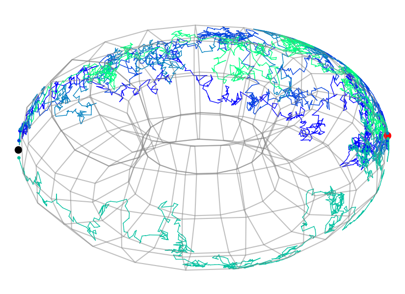
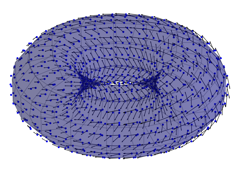
Refer to caption
(a) Four sample paths from the simulation scheme of the radial bridge, Xtsubscript𝑋𝑑X_{t}, from xπ‘₯x (red point) to v𝑣v (black point).
Refer to caption
(b) Radial vector field on the torus, related to the radial bridge, Xtsubscript𝑋𝑑X_{t}, centered at the point XT=vsubscript𝑋𝑇𝑣X_{T}=v.
Figure 3:

In the second example, we consider another two-dimensional manifold, namely the cylinder β„³=π•Š1×ℝℳsuperscriptπ•Š1ℝ\mathcal{M}=\mathbb{S}^{1}\times\mathbb{R}. On the cylinder, the cut locus of a point v=(p,x)βˆˆπ•Š1×ℝ𝑣𝑝π‘₯superscriptπ•Š1ℝv=(p,x)\in\mathbb{S}^{1}\times\mathbb{R} is the set Cut⁑(v)={q}×ℝCutπ‘£π‘žβ„\operatorname{Cut}(v)=\{q\}\times\mathbb{R}, where qβˆˆπ•Š1π‘žsuperscriptπ•Š1q\in\mathbb{S}^{1} is antipodal to p𝑝p. This is illustrated in Figure 2.

Refer to caption
Figure 4: An example of four sample paths of the radial bridge conditioned to arrive at a point in the cut locus, Cut⁑(x)Cutπ‘₯\operatorname{Cut}(x), of the initial point xπ‘₯x.

Any winding around the cylinder trivially makes the process cross the cut locus. In Figure 4, we illustrate the radial bridge’s sample paths ending up at the cut locus at the terminal time winding different ways around the cylinder.

In the third example, we show how our simulation scheme works on a three-dimensional manifold. We consider the special orthogonal group SO​(3)SO3\mathrm{SO}(3) consisting of 3Γ—3333\times 3 orthogonal matrices of determinant 1. Figure 5 shows sample paths of the radial bridge from x∈S​O​(3)π‘₯𝑆𝑂3x\in SO(3) to v∈S​O​(3)𝑣𝑆𝑂3v\in SO(3), where x=Id3π‘₯subscriptId3x=\mathrm{Id}_{3} (columns: red, blue, green vectors) and v𝑣v (black) is the terminal value XT=vsubscript𝑋𝑇𝑣X_{T}=v.

Refer to caption
(a)
Refer to caption
(b)
Refer to caption
(c)
Figure 5: The figure illustrates three sample paths from the radial bridge on S​O​(3)𝑆𝑂3SO(3), by showing its left action on a basis of ℝ3superscriptℝ3\mathbb{R}^{3}. The black arrows indicate the conditioned point.

7.2 Bridge simulation for density estimation on 2-Sphere

Bridge sampling can be used to estimate the transition density of a stochastic process. Assume that the family {Ο†t:t∈[0,T)}conditional-setsubscriptπœ‘π‘‘π‘‘0𝑇\{\varphi_{t}\colon t\in[0,T)\} is uniformly integrable. As is seen from LemmaΒ 6.2

𝔼​[Ctβ€‹Οˆt]β€‹βŸΆtβ†’T​p​(0,x0;T,v)​det(G​(v))β€‹βˆ«Ο•β€‹(β„³)eβˆ’12​βˆ₯Οƒβˆ’1​(T,0)​uβˆ’1​(βˆ‡d​(Ο•βˆ’1​(y),v)22)βˆ₯2​𝑑y,𝔼delimited-[]subscript𝐢𝑑subscriptπœ“π‘‘β†’π‘‘π‘‡βŸΆπ‘0subscriptπ‘₯0𝑇𝑣𝐺𝑣subscriptitalic-Ο•β„³superscript𝑒12superscriptdelimited-βˆ₯βˆ₯superscript𝜎1𝑇0superscript𝑒1βˆ‡π‘‘superscriptsuperscriptitalic-Ο•1𝑦𝑣222differential-d𝑦\mathbb{E}[C_{t}\psi_{t}]\overset{t\rightarrow T}{\longrightarrow}p(0,x_{0};T,v)\sqrt{\det(G(v))}\int_{\phi(\mathcal{M})}e^{-\frac{1}{2}\big{\lVert}\sigma^{-1}(T,0)u^{-1}\left(\frac{\nabla d(\phi^{-1}(y),v)^{2}}{2}\right)\big{\rVert}^{2}}dy,

which in the case of the d𝑑d-sphere can be expressed as

𝔼​[Ctβ€‹Οˆt]𝔼delimited-[]subscript𝐢𝑑subscriptπœ“π‘‘\displaystyle\mathbb{E}[C_{t}\psi_{t}] ⟢tβ†’T​p​(0,x0;T,v)​det(G​(v))β€‹βˆ«β„deβˆ’12​yT​A​(T,0)​y​𝑑yβ†’π‘‘π‘‡βŸΆπ‘0subscriptπ‘₯0𝑇𝑣𝐺𝑣subscriptsuperscriptℝ𝑑superscript𝑒12superscript𝑦𝑇𝐴𝑇0𝑦differential-d𝑦\displaystyle\overset{t\rightarrow T}{\longrightarrow}p(0,x_{0};T,v)\sqrt{\det(G(v))}\int_{\mathbb{R}^{d}}e^{-\frac{1}{2}y^{T}A(T,0)y}dy
=p​(0,x0;T,v)​(2​π)2​det(G​(v))det(A​(T,0)),absent𝑝0subscriptπ‘₯0𝑇𝑣superscript2πœ‹2𝐺𝑣𝐴𝑇0\displaystyle=\frac{p(0,x_{0};T,v)\sqrt{(2\pi)^{2}}\sqrt{\det\left(G(v)\right)}}{\sqrt{\det\left(A(T,0)\right)}},

From the identity linking Ο†tsubscriptπœ‘π‘‘\varphi_{t} to ψtsubscriptπœ“π‘‘\psi_{t}, this leads to the following expression for the transition density with respect to the Riemannian volume form

p​(0,x0;T,v)=det(A​(T,0))(2​π​T)d​eβˆ’12​βˆ₯Οƒβˆ’1​(T,x0)​uβˆ’1​(βˆ‡d​(x0,v)22)βˆ₯2​𝔼​[Ο†T],𝑝0subscriptπ‘₯0𝑇𝑣𝐴𝑇0superscript2πœ‹π‘‡π‘‘superscript𝑒12superscriptdelimited-βˆ₯βˆ₯superscript𝜎1𝑇subscriptπ‘₯0superscript𝑒1βˆ‡π‘‘superscriptsubscriptπ‘₯0𝑣222𝔼delimited-[]subscriptπœ‘π‘‡p(0,x_{0};T,v)=\frac{\sqrt{\det\left(A(T,0)\right)}}{\sqrt{(2\pi T)^{d}}}e^{-\frac{1}{2}\big{\lVert}\sigma^{-1}(T,x_{0})u^{-1}\left(\frac{\nabla d(x_{0},v)^{2}}{2}\right)\big{\rVert}^{2}}\mathbb{E}[\varphi_{T}],

see also [26]. In the Brownian motion setting, the above simplifies to

p​(0,x0;T,v)=1(2​π​T)d​eβˆ’rt22​T​𝔼​[Ο†T].𝑝0subscriptπ‘₯0𝑇𝑣1superscript2πœ‹π‘‡π‘‘superscript𝑒superscriptsubscriptπ‘Ÿπ‘‘22𝑇𝔼delimited-[]subscriptπœ‘π‘‡p(0,x_{0};T,v)=\frac{1}{\sqrt{(2\pi T)^{d}}}e^{-\frac{r_{t}^{2}}{2T}}\mathbb{E}[\varphi_{T}]. (23)

Thus, we obtain an expression for the transition density of the Brownian motion.

On the sphere, we also have series expansions for the heat kernel as uniformly and absolute convergent power series

p​(0,x;t,y)=βˆ‘l=0∞eβˆ’l​(l+dβˆ’1)​t​2​l+dβˆ’1dβˆ’1​1Aπ•Šd​Cld2βˆ’1​(⟨x,yβŸ©β„d+1),𝑝0π‘₯𝑑𝑦superscriptsubscript𝑙0superscript𝑒𝑙𝑙𝑑1𝑑2𝑙𝑑1𝑑11subscript𝐴superscriptπ•Šπ‘‘superscriptsubscript𝐢𝑙𝑑21subscriptπ‘₯𝑦superscriptℝ𝑑1p(0,x;t,y)=\sum_{l=0}^{\infty}e^{-l(l+d-1)t}\frac{2l+d-1}{d-1}\frac{1}{A_{\mathbb{S}^{d}}}C_{l}^{\frac{d}{2}-1}(\langle x,y\rangle_{\mathbb{R}^{d+1}}), (24)

for x,yβˆˆπ•Šdπ‘₯𝑦superscriptπ•Šπ‘‘x,y\in\mathbb{S}^{d}, where ClΞ±superscriptsubscript𝐢𝑙𝛼C_{l}^{\alpha} are the Gegenbauer polynomials and Aπ•Šd=2​π(d+1)/2Γ​((d+1)/2)subscript𝐴superscriptπ•Šπ‘‘2superscriptπœ‹π‘‘12Γ𝑑12A_{\mathbb{S}^{d}}=\frac{2\pi^{(d+1)/2}}{\Gamma((d+1)/2)} the surface area of π•Šdsuperscriptπ•Šπ‘‘\mathbb{S}^{d} [37]. In Figure 6, we have plotted the transition density estimated from (23) using sampling to approximate 𝔼​[Ο†T]𝔼delimited-[]subscriptπœ‘π‘‡\mathbb{E}[\varphi_{T}] against a truncated version (l=0,…,16𝑙0…16l=0,\ldots,16) of (24) as well as the density for the two-dimensional Euclidean Brownian motion. We have plotted the estimated densities along a geodesic running from the north pole to the south pole for three time points, T=0.5,1,1.5𝑇0.511.5T=0.5,1,1.5.

Refer to caption
Figure 6: Estimated transition densities of a Brownian motion (red) on π•Š2superscriptπ•Š2\mathbb{S}^{2} using (23) with T=0.5,1,2𝑇0.512T=0.5,1,2. The densities are computed along a geodesic from the north-pole to the south-pole. The estimated densities are compared to an approximation using (24) (blue) on π•Š2superscriptπ•Š2\mathbb{S}^{2} and densities of a 222-dimensional Euclidean Brownian motion (green).

The resulting estimated heat kernel on π•Š2superscriptπ•Š2\mathbb{S}^{2}, using the sampling scheme above, is displayed in Figure 7.
Refer to caption
Refer to caption
Refer to caption
Figure 7: Estimated transition density on the 222-sphere at times T=t𝑇𝑑T=t, for t=1/2,3/4,1𝑑12341t=1/2,3/4,1, respectively.

Figure 8 shows the estimated heat kernel on a ellipsoid where no closed form solution is directly available. Figure 9 shows the estimated heat kernel on the torus 𝕋2superscript𝕋2\mathbb{T}^{2}.

Refer to caption
Refer to caption
Refer to caption
Figure 8: Estimated transition density on ellipsoid at times T=t𝑇𝑑T=t, for t=1/2,3/4,1𝑑12341t=1/2,3/4,1, respectively.
Refer to caption
Refer to caption
Refer to caption
Figure 9: Estimated transition density on the embedded torus 𝕋2superscript𝕋2\mathbb{T}^{2} at times T=t𝑇𝑑T=t, for t=1/2,3/4,1𝑑12341t=1/2,3/4,1, respectively.

7.3 Bridge simulation for diffusion mean estimation

We now demonstrate how the bridge sampling scheme can be used to estimate diffusion means [16, 17] on the two-sphere. As described in the previous section, bridge sampling can be used to estimate the transition density of a Brownian motion. Using the approximation of the transition density (23) with sampling to approximate the expectation over Ο†Tsubscriptπœ‘π‘‡\varphi_{T}, we can compute likelihood that make up the objective function for the diffusion mean. We can compute gradients of this quantity with respect to the initial valued and perform iterative optimization to find the diffusion mean.

In figure 10(a), we sampled 100 points on π•Š2superscriptπ•Š2\mathbb{S}^{2} from a Brownian motion at t=1𝑑1t=1. Figure 10(b) illustrates how the initial guess of the mean (black dot) converges to the true mean (red dot) using an iterative optimization of the likelihood. From figure 10(c), we see how the iterated likelihood obtained converges.
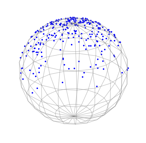
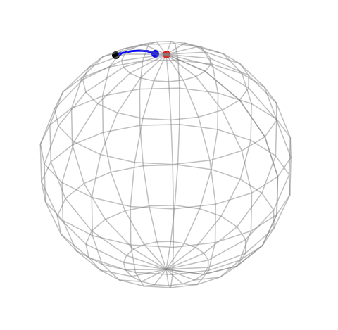
Refer to caption
(a) Sampled data points on π•Š2superscriptπ•Š2\mathbb{S}^{2}.
Refer to caption
(b) Convergence to the diffusion mean (red dot) on π•Š2superscriptπ•Š2\mathbb{S}^{2} from initial guess (black dot).
Refer to caption
(c) The iterated likelihood.
Figure 10: The diffusion mean on π•Š2superscriptπ•Š2\mathbb{S}^{2} is estimated using our bridge sampling scheme. We sampled 100 points on π•Š2superscriptπ•Š2\mathbb{S}^{2} as endpoints of a Brownian motion started at the north pole. Using an initial guess of the mean, we sampled one bridge per observation to obtain an estimate for the likelihood and from this perform iterative optimization to maximize the likelihood. The iterative maximum likelihood approach yields a fast convergence after approximately 20 iterations.

Acknowledgements

The presented research was supported by the CSGB Centre for Stochastic Geometry and Advanced Bioimaging funded by a grant from the Villum Foundation. S. Sommer is supported by the Villum Foundation Grants 40582 and the Novo Nordisk Foundation grant NNF18OC0052000.

References

  • [1] A. Arnaudon, D.D. Holm, A. Pai, and S. Sommer, A stochastic large deformation model for computational anatomy, in International Conference on Information Processing in Medical Imaging. Springer, 2017, pp. 571–582.
  • [2] A. Arnaudon, D.D. Holm, and S. Sommer, A geometric framework for stochastic shape analysis, Foundations of Computational Mathematics 19 (2019), pp. 653–701.
  • [3] A. Arnaudon, F. vanΒ der Meulen, M. Schauer, and S. Sommer, Diffusion Bridges for Stochastic Hamiltonian Systems and Shape Evolutions, SIAM Journal on Imaging Sciences 15 (2022), pp. 293–323.
  • [4] D. Barden and H. Le, Some consequences of the nature of the distance function on the cut locus in a riemannian manifold, Journal of the LMS (1997), pp. 369–383.
  • [5] M. Bladt, S. Finch, and M. SΓΈrensen, Simulation of multivariate diffusion bridges, Journal of the Royal Statistical Society: Series B: Statistical Methodology (2016), pp. 343–369.
  • [6] M. Bladt, M. SΓΈrensen, etΒ al., Simple simulation of diffusion bridges with application to likelihood inference for diffusions, Bernoulli 20 (2014), pp. 645–675.
  • [7] M.N. Bui, Inference on Riemannian Manifolds: Regression and Stochastic Differential Equations, Doctoral, UCL (University College London), 2022.
  • [8] M.N. Bui, Y. Pokern, and P. Dellaportas, Inference for partially observed Riemannian Ornstein-Uhlenbeck diffusions of covariance matrices (2022). arXiv:2104.03193 [stat].
  • [9] J. Clark, The simulation of pinned diffusions, in 29th IEEE Conference on Decision and Control. IEEE, 1990, pp. 1418–1420.
  • [10] B. Delyon and Y. Hu, Simulation of conditioned diffusion and application to parameter estimation, Stochastic Processes and their Applications (2006).
  • [11] D. Elworthy, Geometric aspects of diffusions on manifolds, in Γ‰cole d’ÉtΓ© de ProbabilitΓ©s de Saint-Flour XV–XVII, 1985–87, Springer, 1988, pp. 277–425.
  • [12] K. Elworthy and A. Truman, The diffusion equation and classical mechanics: an elementary formula, in Stochastic processes in quantum theory and statistical physics, Springer, 1982, pp. 136–146.
  • [13] K.D. Elworthy, Stochastic differential equations on manifolds, Vol.Β 70, Cambridge University Press, 1982.
  • [14] M. Emery, Stochastic calculus in manifolds, Springer, 1989.
  • [15] A. Gelman and X.L. Meng, Simulating normalizing constants: From importance sampling to bridge sampling to path sampling, Statistical science (1998), pp. 163–185.
  • [16] P. Hansen, B. Eltzner, S.F. Huckemann, and S. Sommer, Diffusion means in geometric spaces, accepted for Bernoulli, arXiv:2105.12061 (2022).
  • [17] P. Hansen, B. Eltzner, and S. Sommer, Diffusion Means and Heat Kernel on Manifolds, in Geometric Science of Information, F. Nielsen and F. Barbaresco, eds., Cham. Springer International Publishing, Lecture Notes in Computer Science, 2021, pp. 111–118.
  • [18] E.P. Hsu, Stochastic analysis on manifolds, Vol.Β 38, AMS, 2002.
  • [19] P. Hsu, Brownian bridges on Riemannian manifolds, Probability Theory and Related Fields 84 (1990), pp. 103–118.
  • [20] M.H. Jensen, A. Mallasto, and S. Sommer, Simulation of Conditioned Diffusions on the Flat Torus, in International Conference on Geometric Science of Information. Springer, 2019, pp. 685–694.
  • [21] W.S. Kendall, The radial part of brownian motion on a manifold: a semimartingale property, The Annals of Probability 15 (1987), pp. 1491–1500.
  • [22] H. Le and D. Barden, ItΓ΄ correction terms for the radial parts of semimartingales on manifolds, Probability theory and related fields 101 (1995), pp. 133–146.
  • [23] X.M. Li, Generalised brownian bridges: examples, arXiv preprint arXiv:1612.08716 (2016).
  • [24] X.M. Li, On hypoelliptic bridge, Electron. Commun. Probab. 21 (2016), p. 12 pp.
  • [25] P. Malliavin and D.W. Stroock, Short time behavior of the heat kernel and its logarithmic derivatives, Journal of Differential Geometry 44 (1996), pp. 550–570.
  • [26] O. Papaspiliopoulos and G. Roberts, Importance sampling techniques for estimation of diffusion models, Statistical methods for stochastic differential equations (2012), pp. 311–340.
  • [27] X. Pennec, S. Sommer, and T. Fletcher, Riemannian Geometric Statistics in Medical Image Analysis, Academic Press, 2019.
  • [28] D. Revuz and M. Yor, Continuous Martingales and Brownian motion, Springer, 1999.
  • [29] M. Schauer, F. Van DerΒ Meulen, H. VanΒ Zanten, etΒ al., Guided proposals for simulating multi-dimensional diffusion bridges, Bernoulli 23 (2017), pp. 2917–2950.
  • [30] S. Sommer, Anisotropically weighted and nonholonomically constrained evolutions on manifolds, Entropy 18 (2016), p. 425.
  • [31] S. Sommer, A. Arnaudon, L. Kuhnel, and S. Joshi, Bridge simulation and metric estimation on landmark manifolds, in Graphs in Biomedical Image Analysis, Computational Anatomy and Imaging Genetics, Springer, 2017, pp. 79–91.
  • [32] D.W. Stroock and J. Turetsky, Short time behavior of logarithmic derivatives of the heat kernel, Asian Journal of Mathematics 1 (1997), pp. 17–33.
  • [33] C.H. Taubes, Differential geometry: Bundles, connections, metrics and curvature, Vol.Β 23, OUP Oxford, 2011.
  • [34] J. Thompson, Submanifold bridge processes, Ph.D. diss., University of Warwick, 2015.
  • [35] J. Thompson, Brownian bridges to submanifolds, Potential Analysis 49 (2018), pp. 555–581.
  • [36] F. vanΒ der Meulen, M. Schauer, etΒ al., Bayesian estimation of discretely observed multi-dimensional diffusion processes using guided proposals, Electronic Journal of Statistics 11 (2017), pp. 2358–2396.
  • [37] C. Zhao and J.S. Song, Exact heat kernel on a hypersphere and its applications in kernel svm, Frontiers in Applied Mathematics and Statistics 4 (2018), p.Β 1.