\ul
Precise Approximation of Convolutional Neural Networks for Homomorphically Encrypted Data
Abstract
Homomorphic encryption is one of the representative solutions to privacy-preserving machine learning (PPML) classification enabling the server to classify private data of clients while guaranteeing privacy. This work focuses on PPML using word-wise fully homomorphic encryption (FHE). In order to implement deep learning on word-wise homomorphic encryption (HE), the ReLU and max-pooling functions should be approximated by some polynomials for homomorphic operations. Most of the previous studies focus on HE-friendly networks, where the ReLU and max-pooling functions are approximated using low-degree polynomials. However, for the classification of the CIFAR-10 dataset, using a low-degree polynomial requires designing a new deep learning model and training. In addition, this approximation by low-degree polynomials cannot support deeper neural networks due to large approximation errors. Thus, we propose a precise polynomial approximation technique for the ReLU and max-pooling functions. Precise approximation using a single polynomial requires an exponentially high-degree polynomial, which results in a significant number of non-scalar multiplications. Thus, we propose a method to approximate the ReLU and max-pooling functions accurately using a composition of minimax approximate polynomials of small degrees. If we replace the ReLU and max-pooling functions with the proposed approximate polynomials, well-studied deep learning models such as ResNet and VGGNet can still be used without further modification for PPML on FHE. Even pre-trained parameters can be used without retraining. We approximate the ReLU and max-pooling functions in the ResNet-152 using the composition of minimax approximate polynomials of degrees 15, 27, and 29. Then, we succeed in classifying the plaintext ImageNet dataset with 77.52% accuracy, which is very close to the original model accuracy of 78.31%.
1 Introduction
One of the most promising areas in privacy-preserving machine learning (PPML) is deep learning using homomorphic encryption (HE). HE is a cryptographic system that allows algebraic operations such as addition and multiplication on encrypted data. Using HE, the server can perform deep learning on the encrypted data from the client while fundamentally preventing the privacy leakage of private data. Recently, deep learning using HE has been studied extensively [1, 2, 3, 4, 5, 6, 7]. These studies can be classified into deep learning studies using only HE and those using both HE and multi-party computation (MPC) techniques together. Our work focuses on the former, which has advantages of low communication cost and no risk of model exposure compared to hybrid methods using both HE and MPC techniques. In particular, we focus on deep learning using the word-wise fully homomorphic encryption (FHE), which allows the addition and multiplication of an encrypted array over the set of complex numbers or for an integer without restriction on the number of operations.
In word-wise FHE, the ReLU and max-pooling functions cannot be performed on the encrypted data because they are non-arithmetic operations. Thus, after the approximate polynomials replace the ReLU and max-pooling functions, deep learning on the encrypted data can be performed. Most of the previous studies of deep learning on HE focus on HE-friendly networks, where the ReLU and max-pooling functions are approximated using low-degree polynomials. These studies on HE-friendly networks have some limitations. For instance, designing a new deep learning model and training are required in [5, 7, 8], which classified the CIFAR-10 [9]. However, in many real-world applications, training data or training frameworks are not accessible, and thus, the previously studied low-degree approximate polynomials cannot be used in these applications. Furthermore, HE-friendly networks cannot support very deep neural networks due to large approximation errors. On the other hand, the computational time and accuracy of bootstrapping in word-wise FHE have recently been improved significantly [10, 26, 12, 13], allowing the evaluation of higher-degree polynomials for many times. Thus, it is essential to study precise approximate polynomials.
1.1 Our contributions
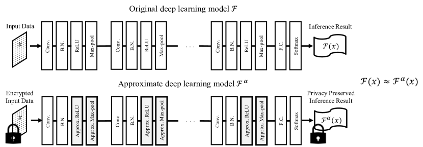
Precise approximation requires a polynomial of degree at least about for the precision parameter , which results in number of non-scalar multiplications and several numerical issues (see Section 3.3). Thus, we propose a precise polynomial approximation technique for the ReLU and max-pooling functions that uses a composition of minimax approximate polynomials of small degrees. Hence, we can replace the ReLU and max-pooling functions with the proposed approximate polynomials in well-studied deep learning models such as ResNet [14], VGGNet [15], and GoogLeNet [16], and the pre-trained parameters can be used without retraining. Figure 1 shows the comparison between the original deep learning model and the proposed approximate deep learning model for the precision parameter , where is the function that outputs the inference result for an input .
We prove that the two inference results, and , satisfy for a constant , which can be determined independently of the precision parameter (see Theorem 4). Theoretically, if we increase the precision parameter enough, the two inference results would be identical. The numerical evaluation also supports that the two inference results are very close for an appropriate .
We classify the CIFAR-10 without retraining using well-studied deep learning models such as ResNet and VGGNet, and pre-trained parameters. We can also further reduce the required precision parameter by allowing retraining for only a few epochs. For classifying the ImageNet [17] in ResNet-152, we approximate the ReLU and max-pooling functions using the composition of minimax approximate polynomials of degrees 15, 27, and 29. Then, for the first time for PPML using word-wise HE, we successfully classify the ImageNet with 77.52% accuracy, which is very close to the original model accuracy of 78.31%. The proposed approximate polynomials are generally applicable to various deep learning models such as ResNet, VGGNet, and GoogLeNet for PPML on FHE.
1.2 Related works
Deep learning on the homomorphically encrypted data, i.e., PPML using HE, can be classified into two categories: One uses HE only, and the other uses HE and MPC techniques together. Gazelle [2], Cheetah [6], and nGraph-HE [4] are representative studies that perform deep learning using HE and MPC techniques together. They used garbled circuits to perform activation functions through communication with clients and servers. However, the use of MPC techniques can lead to high communication costs or disclose information on the configuration of the deep learning models.
PPML using only HE can be classified into PPML using bit-wise HE and PPML using word-wise HE. In [18], PPML using the fast fully homomorphic encryption over the torus (TFHE) [19], which is the most promising bit-wise FHE, was studied. This PPML can evaluate the ReLU and max-pooling functions exactly on the encrypted data. However, leveled HE was used instead of FHE because of the large computational time of FHE operations, which limits performing a very deep neural network on HE. Our work focuses on deep learning using word-wise FHE such as the Brakerski/Fan-Vercauteren [20] and Cheon-Kim-Kim-Song (CKKS) scheme [21]. CryptoNets [1], Faster CryptoNets [5], SEALion [3], and studies in [7, 8] also performed deep learning using word-wise HE. By designing a new deep learning model and training, the authors in [5], [7], and [8] classified the CIFAR-10 with an accuracy of about , , and , respectively. CryptoNets and SEALion replaced the ReLU function with square function , and Faster CryptoNets replaced the ReLU function with quantized minimax approximate polynomial .
2 Preliminaries
2.1 Minimax composite polynomial
Unfortunately, FHE schemes do not support non-arithmetic operations such as sign function, where for , and , otherwise. Hence, instead of the actual sign function, a polynomial approximating the sign function should be evaluated on the encrypted data. Recently, authors in [22] proposed a composite polynomial named minimax composite polynomial that optimally approximates the sign function with respect to the depth consumption and the number of non-scalar multiplications. The definition of minimax composite polynomial is given as follows:
Definition 1.
Let be . A composite polynomial is called a minimax composite polynomial on for if the followings are satisfied:
-
•
is the minimax approximate polynomial of degree at most on for .
-
•
For , is the minimax approximate polynomial of degree at most on for .
2.2 Homomorphic max function
To perform the max function on the encrypted data, called the homomorphic max function, a polynomial that approximates the max function should be evaluated on the encrypted data instead of the max function. The approximate polynomial of the max function, , should satisfy the following inequality for the precision parameter :
| (1) |
In [23], considering , they obtained a polynomial that approximates and then used it to determine a polynomial that approximates , that is,
| (2) |
| degrees | depth | ||
|---|---|---|---|
| 4 | 5 | {5} | 4 |
| 5 | 5 | {13} | 5 |
| 6 | 10 | {3,7} | 6 |
| 7 | 11 | {7,7} | 7 |
| 8 | 12 | {7,15} | 8 |
| 9 | 13 | {15,15} | 9 |
| 10 | 13 | {7,7,13} | 11 |
| 11 | 15 | {7,7,27} | 12 |
| 12 | 15 | {7,15,27} | 13 |
| 13 | 16 | {15,15,27} | 14 |
| 14 | 17 | {15,27,29} | 15 |
In [22], the authors proposed a minimax composite polynomial approximating the sign function. Then, they proposed a polynomial approximating the max function using and equation (2). Specifically, for a precision parameter and the optimized max function factor , an -close minimax composite polynomial was obtained by using the optimal degrees obtained from Algorithm 5 in [22], where the depth consumption is minimized. Then, it was shown that from satisfies the error condition in equation (1). Table 1 lists the values of , corresponding depth consumption for evaluating , and degrees of the component polynomials according to . This approximate polynomial has the best performance up to now.
3 Precise polynomial approximation of the ReLU and max-pooling functions
It is possible to approximate the ReLU and max-pooling functions by Taylor polynomials or minimax approximate polynomials [24]. However, these approximate polynomials with minimal approximation errors require many non-scalar multiplications. For this reason, we approximate the ReLU and max-pooling functions using and , which are defined in Section 2.2. Although we only deal with the ReLU function among many activation functions, the proposed approximation method can also be applied to other activation functions such as the leaky ReLU function.
3.1 Precise approximate polynomial of the ReLU function
In this subsection, we propose a polynomial that precisely approximates the ReLU function, a key component of deep neural networks. For a given precision parameter , it is required that the approximate polynomial of the ReLU function, , satisfies the following error condition:
| (3) |
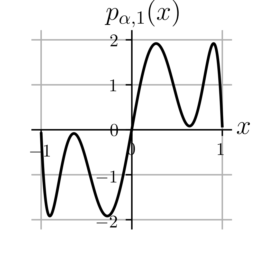
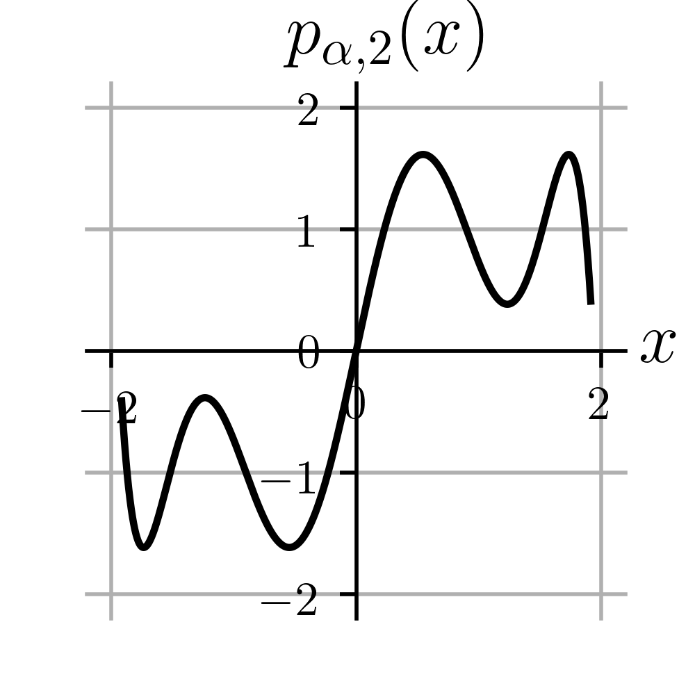
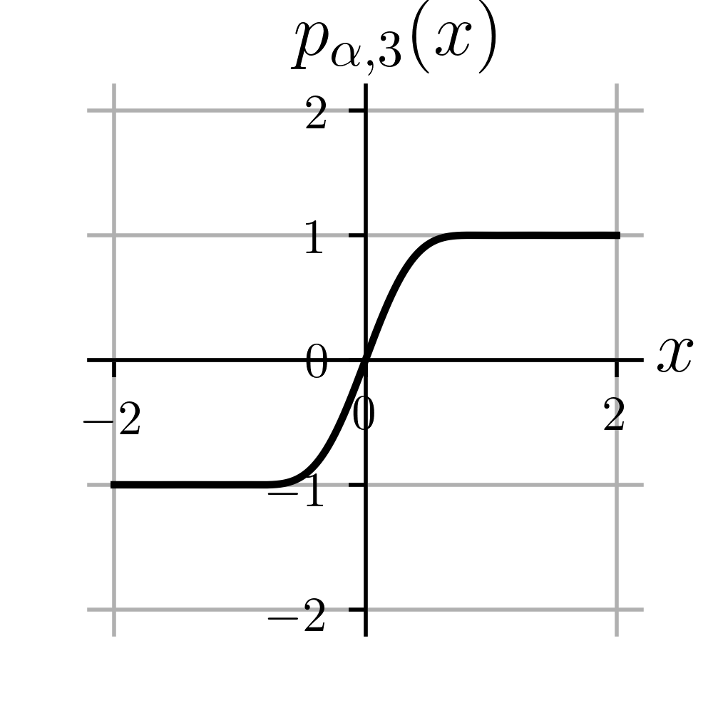
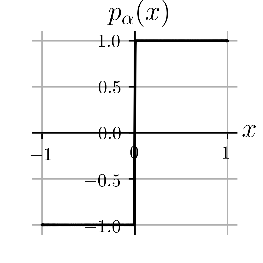
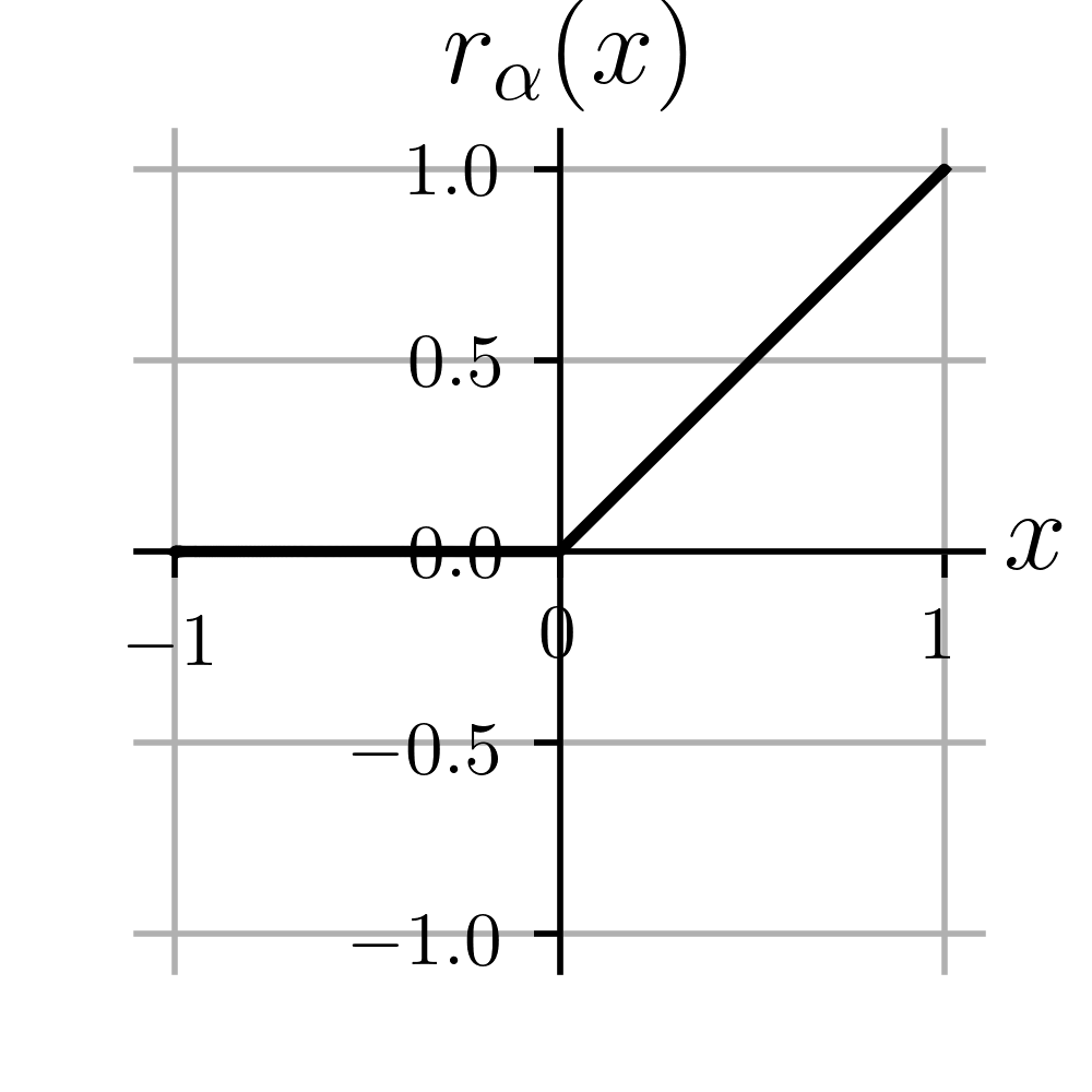
It is well-known that . Then, we propose the following approximate polynomial of the ReLU function, . The specific coefficient values of for several can be seen in Appendix A. Figure 2 shows the component polynomials of and the proposed with the precision parameter . The following theorem shows that the proposed satisfies the error condition of the ReLU function in equation (3).
Theorem 1.
For any , satisfies the following inequality:
The proofs of all theorems and a lemma are given in Appendix B.
Approximation range
The value of polynomial is close to the ReLU function value only for . However, since some input values of the ReLU function during deep learning are not in , the approximation range should be extended from to a larger range for some . Thus, we propose a polynomial approximating the ReLU function in the range . Then, we have for . Large has the advantage of enlarging input ranges of the ReLU function at the cost of causing a larger approximation error with the ReLU function.
3.2 Precise approximate polynomial of the max-pooling function
The max-pooling function with kernel size outputs the maximum value among input values. To implement the max-pooling function for the homomorphically encrypted data, we should find a polynomial that approximates the max-pooling function.
We define a polynomial that approximates the maximum value function using . To reduce the depth consumption of the approximate polynomial of the max-pooling function, we construct by compositing polynomial with a minimal number of compositions. We use the following recursion equation to obtain the approximated maximum value among :
| (4) |
The following theorem shows the upper bound of approximation error of .
Theorem 2.
For given and , the polynomial obtained from the recursion equation in (4) satisfies
| (5) | ||||
Approximation range
To extend the approximation range to for , we use the following polynomial as an approximation polynomial:
where . Then, we have
for , which directly follows from Theorem 2.
3.3 Comparison between the minimax approximate polynomial and the proposed approximate polynomial for the ReLU and max-pooling functions
One can think that precise approximation of the ReLU function can be achieved simply by using a high-degree polynomial such as a Taylor polynomial and minimax approximate polynomial [24]. In particular, the minimax approximate polynomials have the minimum minimax error for a given degree. Thus, the minimax approximate polynomials are good candidates for the approximate polynomials. In this subsection, we compare the proposed approximation method using and the method using the minimax approximate polynomial. For simplicity, let the approximation range of the ReLU function be . Then, for a given degree , the minimax approximate polynomial of degree at most on for can be obtained from the Remez algorithm [24]. The precision parameter corresponds to the logarithm of the minimax error using base two. Figure 3 presents the corresponding precision parameter according to the logarithm of the polynomial degree (base two). Because performing the Remez algorithm for a high-degree polynomial has several difficulties , such as using high real number precision and finding extreme points with high precision, we obtain the polynomials for only up to degree . It can be seen that and have an almost exact linear relationship, and we obtain the following regression equation:
| (6) |
Table 2 compares the approximation method using the minimax approximate polynomial and that using the proposed approximate polynomial . The required number of non-scalar multiplications for evaluating a polynomial of degree is [25], and thus, non-scalar multiplications are required for the precision parameter . The exact number of non-scalar multiplications is obtained using the odd baby-step giant-step algorithm for polynomials with only odd-degree terms and using the optimized baby-step giant-step algorithm for other polynomials [11]. From Table 2, it can be seen that the minimax approximate polynomial of exponentially high degree is required for a large . This high degree requires many non-scalar multiplications, i.e., large computational time. In addition, using a high-degree polynomial has some numerical issues, such as the requirement of high precision of the real number. Thus, precise approximation using the minimax approximate polynomial is inefficient to use in practice.
| minimax | proposed | |||
|---|---|---|---|---|
| approx. polynomial | approx. polynomial | |||
| degree | #mults | degrees | #mults | |
| 6 | 10 | 5 | {3,7} | 7 |
| 7 | 20 | 8 | {7,7} | 9 |
| 8 | 40 | 12 | {7,15} | 12 |
| 9 | 80 | 18 | {15,15} | 15 |
| 10 | 150 | 25 | {7,7,13} | 16 |
| 11 | 287* | 35 | {7,7,27} | 19 |
| 12 | 575* | 49 | {7,15,27} | 22 |
| 13 | 1151* | 70 | {15,15,27} | 25 |
| 14 | 2304* | 98 | {15,27,29} | 28 |
| 15 | 4612* | 140 | {29,29,29} | 30 |
Homomorphic max function
Considering , we obtain the minimax approximate polynomial on for . Then, can be used as an approximate polynomial of the max function . Since , the approximation of and are equivalent. Thus, when the max function is approximated with the minimax approximate polynomial, an exponentially large degree is also required to achieve large .
4 Theoretical performance analysis of approximate deep learning model
In this section, we propose an approximate deep learning model for homomorphically encrypted input data, replacing the original ReLU and max-pooling functions with the proposed precise approximate polynomials and in the original deep learning model. In addition, we analytically derive that if the pre-trained parameters of the original deep learning model are available, classification would be accurate if we adopt a proper precision parameter .
In more detail, we estimate the L-infinity norm of the difference between the inference results and , . Here, and denote the inference results of the original deep learning model and the proposed approximate deep learning model with the precision parameter , respectively. Here, and share the same pre-trained parameters. The main conclusion of this section is that we can reduce the difference by increasing , which implies that the proposed model shows almost the same performance as the original pre-trained model.
To estimate , we attempt to decompose the original deep learning model, analyze each component, and finally re-combine them. First, we decompose given deep learning model as , where is called a block. Each block can be a simple function: convolution, batch normalization, activation function, and pooling function. It can also be a mixed operation that cannot be decomposed into simple operations. Here, all of the inputs and outputs of block ’s are considered as a one-dimensional vector. Also, we denote as the corresponding approximate polynomial operation of each block with precision parameter . If block contains only a polynomial operation, is the same as since there is nothing to approximate. Then, the approximate model can be considered as a composition of approximate blocks, .
If there is only a single approximate block in the approximate deep learning model, the difference in inference results can be easily determined. However, the model composed of more than two approximate blocks makes the situation more complicated. Consider an input vector , two consecutive blocks and , and their approximation and . The block makes an approximation error which can be measured as . For a given input , the magnitude of the error is only determined by the intrinsic feature of block . However, the output error of the second block is quite different. Note that we can write the second block error as , where and . Considering , both block and the magnitude of affect the second block error. Then, we define a new measure for each block, error propagation function.
In this study, all inputs in the deep learning models belong to a bounded set for a given dataset. We should set the approximation range for the proposed approximate polynomials for the ReLU and max-pooling functions. We assume that we can choose a sufficiently large such that the inputs of all blocks fall in . That is, for a given deep learning model and the corresponding approximate model , we have and for and every input . In fact, we confirm through numerical analysis that these are satisfied for an appropriately large in Section 5. We define error propagation function as follows:
Definition 2.
For a block , an error propagation function of , , is defined as , where denotes the magnitude of output error of the previous block of .
Roughly speaking, block propagates the input error (or the output error of the previous block) to output error . With this error propagation function, we can estimate the difference between final inference results of and straightforward as in the following theorem.
Theorem 3.
If the original model can be decomposed as , then we have
for every input .
This theorem asserts that we can achieve an upper bound of inference error of the whole model by estimating an error propagation function for each block.
We analyze the error propagation function for four types of single blocks: i) linear block, ii) ReLU block, iii) max-pooling block, and iv) softmax block, commonly used in deep neural networks for classification tasks. From now on, we call these four types of blocks basic blocks for convenience. Note that convolutional layers, batch normalization layers (for inference), average pooling layers, and fully connected layers are just linear combinations of input vectors and model parameters. Therefore, it is reasonable to include all these layers in a linear block. We can express linear blocks as for some matrix and vector . The following lemma shows practical upper bounds of error propagation function for basic blocks. Because the kernel size of the max-pooling function is not greater than ten in most applications, we constrain the kernel size not greater than ten in the following lemma.
Lemma 1.
For the given error , the error propagation functions of four basic blocks are upper bounded as follows: (a) If is a linear block with , then , where denotes the infinity norm of matrices. (b) If is a ReLU block, then . (c) If is a max-pooling block with kernel size and , then . (d) If is a softmax block, then .
Since the upper bounds of error propagation functions of all basic blocks have been determined, we can obtain an upper bound of the inference error theoretically as in the following theorem.
Theorem 4.
If and a deep learning model contains only basic blocks in Lemma 1, then there exists a constant such that for every input , where the constant can be determined independently of the precision parameter .
Therefore, the performance of the proposed approximate deep learning model containing only basic blocks can be guaranteed theoretically by Theorem 4 if the original model is well trained.
Practical application of Theorem 4
Theorem 4 is valid for a deep learning model composed of only basic blocks. VGGNet [15] is a representative example. However, there are also various deep learning models with non-basic blocks. For example, ResNet [14] contains residual learning building block, which is hard to decompose into several basic blocks. Thus, the generalized version of Theorem 4 is presented in Appendix C, which is also valid for ResNet. Numerical results in Section 5 also support that the inference result of the original deep learning model and that of the proposed approximate deep learning model are close enough for a practical precision parameter .
5 Results of numerical analysis
In this section, the simulation results are presented for the original and the proposed approximate deep learning models for the plaintext input data. Overall, our results show that using the large precision parameter obtains high performance in the proposed approximate deep learning model, which confirms Theorem 4. All simulations are proceeded by NVIDIA GeForce RTX 3090 GPU along with AMD Ryzen 9 5950X 16-Core Processor CPU.
5.1 Numerical analysis on the CIFAR-10
Pre-trained backbone models
We use the CIFAR-10 [9] as the input data, which has 50k training images and 10k test images with 10 classes. We use ResNet and VGGNet with batch normalization as backbone models of the proposed approximate deep learning model. To verify that the proposed approximate deep learning models work well for a various number of layers, we use ResNet with 20, 32, 44, 56, and 110 layers and VGGNet with 11, 13, 16, and 19 layers proposed in [14] and [15], respectively. In order to obtain pre-trained parameters for each model, we apply the optimizer suggested in [14] on both ResNet and VGGNet for the CIFAR-10.
Approximation range
The approximation range should be determined in the proposed approximate deep learning model. We examine the input values of the approximate polynomials of the ReLU and max-pooling functions and determine the value of by adding some margin to the maximum of the input values. For the CIFAR-10, we choose for both the approximate polynomials of ReLU and max-pooling functions. However, a larger is required for retraining with ResNet-110 for and . Thus, in the case of retraining with ResNet-110, we use , and for and , respectively.
Numerical results
| Backbone | Baseline(%) | 7 | 8 | 9 | 10 | 11 | 12 | 13 | 14 |
|---|---|---|---|---|---|---|---|---|---|
| ResNet-20 | 88.36 | 10.00 | 10.00 | 10.00 | 19.96 | 80.91 | 86.44 | 88.01 | 88.41 |
| ResNet-32 | 89.38 | 10.00 | 10.00 | 10.01 | 36.16 | 84.92 | 88.08 | 88.99 | 89.23 |
| ResNet-44 | 89.41 | 10.00 | 10.00 | 10.00 | 38.35 | 85.75 | 88.31 | 89.31 | 89.37 |
| ResNet-56 | 89.72 | 10.00 | 10.00 | 9.94 | 39.48 | 86.54 | 89.18 | 89.53 | 89.67 |
| ResNet-110 | 89.87 | 10.00 | 10.00 | 10.04 | 67.02 | 86.75 | 89.17 | 89.62 | 89.84 |
| VGG-11 | 90.17 | 10.77 | 11.74 | 15.61 | 29.39 | 66.60 | 85.22 | 88.95 | 89.91 |
| VGG-13 | 91.90 | 11.32 | 11.57 | 14.37 | 36.84 | 77.55 | 88.72 | 90.66 | 91.37 |
| VGG-16 | 91.99 | 10.02 | 10.06 | 10.76 | 32.93 | 78.27 | 89.69 | 91.13 | 91.87 |
| VGG-19 | 91.75 | 10.18 | 13.84 | 18.18 | 43.56 | 80.40 | 89.42 | 91.10 | 91.61 |
First of all, neither the activation functions , suggested in [1] and [3], nor , suggested in [5], shows good performance in our backbone models. These activation functions give the inference results around 10.0% with our pre-trained parameters. Also, ResNet and VGGNet cannot be trained by the activation functions and , since these activation functions cause a more significant gradient exploding problem as the original model gets deeper. Therefore, a polynomial with a small degree is inappropriate to utilize the pre-trained model, which implies the importance of the proposed precise approximate polynomial for PPML in ResNet and VGGNet.
The inference results of the proposed approximate deep learning models are given in Table 3. Table 3 shows that if we adopt a large precision parameter , the proposed model becomes more accurate, confirming Theorem 4. We achieve the polynomial-operation-only VGG-16 model with 91.87% accuracy for the CIFAR-10 using . In addition, the proposed approximate deep learning model performs almost similarly (1% difference) to the original deep learning model when –.
| Backbone | Baseline | 7 | 8 | 9 | 10 |
|---|---|---|---|---|---|
| ResNet-20 | 88.36 | 80.28 | 84.83 | 86.76 | 86.61 |
| ResNet-32 | 89.38 | 80.09 | 86.08 | 87.76 | 87.85 |
| ResNet-44 | 89.41 | 76.13 | 82.93 | 85.61 | 88.06 |
| ResNet-56 | 89.72 | 70.90 | 77.59 | 85.06 | 87.96 |
| ResNet-110 | 89.87 | 50.47 | 31.24 | 79.93 | 88.28 |
| VGG-11 | 90.17 | 66.54 | 78.57 | 86.56 | 88.04 |
| VGG-13 | 91.90 | 73.09 | 83.67 | 88.97 | 90.74 |
| VGG-16 | 91.99 | 73.75 | 84.12 | 89.37 | 90.65 |
| VGG-19 | 91.75 | 75.54 | 83.77 | 88.90 | 90.21 |
| Backbone | Baseline | Proposed |
|---|---|---|
| Inception-v3 [27] | 69.54 | 69.23 |
| GoogLeNet [16] | 68.13 | 69.76 |
| VGG-19 [15] | 74.22 | 73.46 |
| ResNet-152 [14] | 78.31 | 77.52 |
Moreover, if retraining is allowed for a few epochs, we also obtain high performance in the proposed approximate deep learning model with a smaller precision parameter . We retrain the proposed model using the same optimizer for pre-training but only for ten epochs and drop learning rate with multiplicative factor at the 5th epoch. The results of retraining with precision parameter – are summarized in Table 5. Comparing Tables 3 and 5 shows that the required precision parameter for high classification accuracy is reduced if we allow retraining for ten epochs.
5.2 Numerical analysis on the ImageNet
We also analyze the classification accuracy of the proposed approximate deep learning model for the ImageNet dataset [17], which has 1.28M training images and 50k validation images with 1000 classes. We simulate various models whose pre-trained parameters are available for inference of the ImageNet. For the approximation range , we choose for the ReLU function and for the max-pooling function. The models that we use and their inference results are summarized in Table 5. Without any training, we easily achieve a polynomial-operation-only model with an accuracy of 77.52% for the ImageNet. From this result, it can be seen that even if the dataset is large, the proposed model shows high performance, similar to the original model.
5.3 Discussion of classification accuracy performance on FHE
In this study, deep learning was performed for plaintext input data, not for the homomorphically encrypted input data. However, since polynomials replaced all non-arithmetic operations, the proposed approximate deep learning model can also efficiently be performed in FHE, and the classification accuracy would be identical. In particular, the proposed approximate deep learning model will work well in the RNS-CKKS scheme [28] because the computational time and precision of RNS-CKKS scheme operations have been improved significantly in recent years [10, 26, 12, 13].
6 Conclusion
We proposed the polynomials that precisely approximate the ReLU and max-pooling functions using a composition of minimax approximate polynomials of small degrees for PPML using FHE. We theoretically showed that if the precision parameter is large enough, the difference between the inference result of the original and the proposed approximate models becomes small enough. For the CIFAR-10 dataset, the proposed model approximating ResNet or VGGNet had classification accuracy with only 1% error from the original deep learning model when we used the precision parameter from 12 to 14. Furthermore, for the first time for PPML using word-wise HE, we achieved 77.52% of test accuracy for ImageNet classification, which was close to the original accuracy of 78.31% for the precision parameter .
Appendix
Appendix A Coefficients of the approximate polynomial of the sign function,
In this section, for the approximate polynomial of the sign function, , the coefficients of the component polynomials using the Remez algorithm [24] are shown for the precision parameter . Using the coefficients in the table below, we can obtain the proposed approximate polynomial of the ReLU function using the following equation:
Note that is an odd function theoretically, and the obtained coefficients of even-degree terms of by using the Remez algorithm [24] are almost zero. Even if we delete the even-degree terms of and obtain using the modified , the approximate deep learning model using the modified has almost the same inference results.
| Coefficients of of | |||
| 7 | 1 | 0 | |
| 1 | |||
| 2 | |||
| 3 | |||
| 4 | |||
| 5 | |||
| 6 | |||
| 7 | |||
| 2 | 0 | ||
| 1 | |||
| 2 | |||
| 3 | |||
| 4 | |||
| 5 | |||
| 6 | |||
| 7 | |||
| 8 | 1 | 0 | |
| 1 | |||
| 2 | |||
| 3 | |||
| 4 | |||
| 5 | |||
| 6 | |||
| 7 | |||
| 2 | 0 | ||
| 1 | |||
| 2 | |||
| 3 | |||
| 4 | |||
| 5 | |||
| 6 | |||
| 7 | |||
| 8 | |||
| 9 | |||
| 10 | |||
| 11 | |||
| 12 | |||
| 13 | |||
| 14 | |||
| 15 | |||
| 9 | 1 | 0 | |
| 1 | |||
| 2 | |||
| 3 | |||
| 4 | |||
| 5 | |||
| 6 | |||
| 7 | |||
| 8 | |||
| 9 | |||
| 10 | |||
| 11 | |||
| 12 | |||
| 13 | |||
| 14 | |||
| 15 | |||
| 2 | 0 | ||
| 1 | |||
| 2 | |||
| 3 | |||
| 4 | |||
| 5 | |||
| 6 | |||
| 7 | |||
| 8 | |||
| 9 | |||
| 10 | |||
| 11 | |||
| 12 | |||
| 13 | |||
| 14 | |||
| 15 | |||
| 10 | 1 | 0 | |
| 1 | |||
| 2 | |||
| 3 | |||
| 4 | |||
| 5 | |||
| 6 | |||
| 7 | |||
| 2 | 0 | ||
| 1 | |||
| 2 | |||
| 3 | |||
| 4 | |||
| 5 | |||
| 6 | |||
| 7 | |||
| 3 | 0 | ||
| 1 | |||
| 2 | |||
| 3 | |||
| 4 | |||
| 5 | |||
| 6 | |||
| 7 | |||
| 8 | |||
| 9 | |||
| 10 | |||
| 11 | |||
| 12 | |||
| 13 | |||
| 11 | 1 | 0 | |
| 1 | |||
| 2 | |||
| 3 | |||
| 4 | |||
| 5 | |||
| 6 | |||
| 7 | |||
| 2 | 0 | ||
| 1 | |||
| 2 | |||
| 3 | |||
| 4 | |||
| 5 | |||
| 6 | |||
| 7 | |||
| 3 | 0 | ||
| 1 | |||
| 2 | |||
| 3 | |||
| 4 | |||
| 5 | |||
| 6 | |||
| 7 | |||
| 8 | |||
| 9 | |||
| 10 | |||
| 11 | |||
| 12 | |||
| 13 | |||
| 14 | |||
| 15 | |||
| 16 | |||
| 17 | |||
| 18 | |||
| 19 | |||
| 20 | |||
| 21 | |||
| 22 | |||
| 23 | |||
| 24 | |||
| 25 | |||
| 26 | |||
| 27 | |||
| 12 | 1 | 0 | |
| 1 | |||
| 2 | |||
| 3 | |||
| 4 | |||
| 5 | |||
| 6 | |||
| 7 | |||
| 2 | 0 | ||
| 1 | |||
| 2 | |||
| 3 | |||
| 4 | |||
| 5 | |||
| 6 | |||
| 7 | |||
| 8 | |||
| 9 | |||
| 10 | |||
| 11 | |||
| 12 | |||
| 13 | |||
| 14 | |||
| 15 | |||
| 3 | 0 | ||
| 1 | |||
| 2 | |||
| 3 | |||
| 4 | |||
| 5 | |||
| 6 | |||
| 7 | |||
| 8 | |||
| 9 | |||
| 10 | |||
| 11 | |||
| 12 | |||
| 13 | |||
| 14 | |||
| 15 | |||
| 16 | |||
| 17 | |||
| 18 | |||
| 19 | |||
| 20 | |||
| 21 | |||
| 22 | |||
| 23 | |||
| 24 | |||
| 25 | |||
| 26 | |||
| 27 | |||
| 13 | 1 | 0 | |
| 1 | |||
| 2 | |||
| 3 | |||
| 4 | |||
| 5 | |||
| 6 | |||
| 7 | |||
| 8 | |||
| 9 | |||
| 10 | |||
| 11 | |||
| 12 | |||
| 13 | |||
| 14 | |||
| 15 | |||
| 2 | 0 | ||
| 1 | |||
| 2 | |||
| 3 | |||
| 4 | |||
| 5 | |||
| 6 | |||
| 7 | |||
| 8 | |||
| 9 | |||
| 10 | |||
| 11 | |||
| 12 | |||
| 13 | |||
| 14 | |||
| 15 | |||
| 3 | 0 | ||
| 1 | |||
| 2 | |||
| 3 | |||
| 4 | |||
| 5 | |||
| 6 | |||
| 7 | |||
| 8 | |||
| 9 | |||
| 10 | |||
| 11 | |||
| 12 | |||
| 13 | |||
| 14 | |||
| 15 | |||
| 16 | |||
| 17 | |||
| 18 | |||
| 19 | |||
| 20 | |||
| 21 | |||
| 22 | |||
| 23 | |||
| 24 | |||
| 25 | |||
| 26 | |||
| 27 | |||
| 14 | 1 | 0 | |
| 1 | |||
| 2 | |||
| 3 | |||
| 4 | |||
| 5 | |||
| 6 | |||
| 7 | |||
| 8 | |||
| 9 | |||
| 10 | |||
| 11 | |||
| 12 | |||
| 13 | |||
| 14 | |||
| 15 | |||
| 2 | 0 | ||
| 1 | |||
| 2 | |||
| 3 | |||
| 4 | |||
| 5 | |||
| 6 | |||
| 7 | |||
| 8 | |||
| 9 | |||
| 10 | |||
| 11 | |||
| 12 | |||
| 13 | |||
| 14 | |||
| 15 | |||
| 16 | |||
| 17 | |||
| 18 | |||
| 19 | |||
| 20 | |||
| 21 | |||
| 22 | |||
| 23 | |||
| 24 | |||
| 25 | |||
| 26 | |||
| 27 | |||
| 3 | 0 | ||
| 1 | |||
| 2 | |||
| 3 | |||
| 4 | |||
| 5 | |||
| 6 | |||
| 7 | |||
| 8 | |||
| 9 | |||
| 10 | |||
| 11 | |||
| 12 | |||
| 13 | |||
| 14 | |||
| 15 | |||
| 16 | |||
| 17 | |||
| 18 | |||
| 19 | |||
| 20 | |||
| 21 | |||
| 22 | |||
| 23 | |||
| 24 | |||
| 25 | |||
| 26 | |||
| 27 | |||
| 28 | |||
| 29 |
Appendix B Proofs of theorems and a lemma
Proof of Theorem 1.
Proof.
From the definition, satisfies the following inequality:
for . Then, for , we have . In addition, for , we have . Thus, we have . ∎
Proof of Theorem 2.
Proof.
To prove this theorem, we require two lemmas.
(Lemma (a)) For , let and satisfy
Then, for , the following is satisfied:
(Proof) We will use mathematical induction to show that Lemma (a) holds for all . For , it is trivial because if and only if .
For , we have . We have to show that for . We note that
| (7) |
Because , we have
Also, we have
Thus, Lemma (a) holds for . Now, we assume that Lemma (a) holds for , for some . It is enough to show that Lemma (a) also holds for .
(i)
We have
| (8) |
which is equivalent to Then, we have to show that
for . Because Lemma (a) holds for by the intermediate induction assumption, we have
From the inequality in (8), we have and . Thus, we have
Then, from Lemma (a) for , we have
Thus, Lemma (a) holds for .
(ii)
We have
This is equivalent to
| (9) |
because for every integer . Then, we have to show that
for . Because Lemma (a) holds for and by the intermediate induction assumption, we have
From the inequality in (9) by the intermediate induction assumption, we have and . Thus, we have
Then, from Lemma (a) for , we have
Thus, Lemma (a) holds for . Then, Lemma (a) holds for all by mathematical induction. ∎
(Lemma (b)) For , we have
| (10) |
(Proof) Let without loss of generality. We denote the left-hand side and right-hand side of the inequality in (10) by LHS and RHS, respectively.
-
1.
We have . Thus, the lemma holds in this case. -
2.
We have .-
(a)
We have . Thus, we have . -
(b)
We have . Thus, we have .
-
(a)
Thus, the lemma (b) is proved. ∎
Now, we prove the theorem using Lemma (a) and Lemma (b). We use mathematical induction to show that the inequality in (5) holds for all . First, for , we have
Therefore, the inequality in (5) holds for .
We assume that the inequality holds for all , .
Then, it is enough to show that the inequality in (5) also holds for .
Suppose that .
(i)
We have to show that
We have
Let , , , and . Since
we can apply the intermediate induction assumption for as
The left-hand side of the inequality in (5) for becomes . From Lemma (a) for , we have . Then, we have
(ii)
We have to show that
We have
Let , , , and . Since
we can apply the induction assumption for and as
Proof of Theorem 3.
Proof.
Equivalently, we have to show that
| (11) |
We will prove it by mathematical induction. First, we will prove for .
Thus, the inequality in (11) holds for .
Next, we assume that the inequality in (11) holds for , that is,
for some . It is enough to show that the inequality in (11) also holds for , that is,
We have
Let and . Because , we have
Thus, the inequality in (11) holds for , and the theorem is proved by mathematical induction.
∎
Proof of Lemma 1.
Proof.
(a) For , . Then . Therefore,
(b) For , . Therefore,
(c) If is a max-pooling block with kernel size , becomes
where and . Similar technique of proof for (b) and from Theorem 2, we have , where . Since and , , therefore , which leads the conclusion.
(d) Let us denote softmax block as an function with for . Then mean value theorem for multivariate variable functions gives
where denotes the Jacobian matrix of softmax block . For a given vector , the infinity norm of is given as . Note that
and thus
where . Therefore, for any vector , and this gives
which leads the conclusion. ∎
Proof of Theorem 4.
Proof.
From Theorem 3, it is enough to show that
| (12) |
for some constant and . To show that this inequality holds for all , we use mathematical induction. First, for , assume that has one block . The upper bounds of for the four basic blocks suggested in Lemma 1 have forms of , where can be zero. Thus, the inequality in (12) holds for some constant and .
Then, we assume that the inequality in (12) holds for and some constant , that is, for some . Then, it is enough to show that the inequality in (12) holds for and some constant . is not greater than
-
(i)
when is a linear block with ,
-
(ii)
when is a ReLU block,
-
(iii)
when is a max-pooling block with kernel size ,
-
(iv)
when is a softmax block
by Lemma 1. For each case, we can determine a constant that satisfies . Thus, the theorem is proved. ∎
Appendix C Generalization of Theorem 4 for ResNet model
ResNet model cannot be decomposed of basic blocks, since it contains a “residual block”. The authors of [14] suggest an operation that satisfies
where denotes the residual mapping which will be learned, and is a linear projection matrix to match the dimension of . In this section, we call such operation as a residual block. In the residual block designed in ResNet, all residual mapping is a composition of basic blocks [14]. Therefore, by Theorem 4, we can determine a constant that satisfies . In case of , there are two methods of constructing projection in ResNet: the first one pads extra zeros, and the second one uses convolution [14]. We note that both methods can be considered as linear blocks, and thus the approximate block can be represented by . Considering this situation, we generalize the original Theorem 4 so that it is also valid for ResNet model.
Theorem 5 (generalized version of Theorem 4).
If and a deep learning model contains only basic blocks and residual blocks, then there exists a constant such that for every input , where the constant can be determined only by model parameters.
Proof.
We prove this statement by obtaining error propagation function of residual block . From the definition of error propagation function, we have
where is the constant that satisfies . To estimate , we decompose residual mapping into , where ’s are basic blocks. Then, we define
for a block and magnitude of the error, . Then is a non-decreasing function of for every block . Thus, similar argument in the proof of Theorem 3 shows that
| (13) |
for every error vector . Also, similar argument in the proof of Lemma 1 shows that
| (14) |
for every basic block and . These inequalities for corresponds to the inequalities for in Lemma 1 when the precision parameter goes to infinity. From two inequalities (13) and (14), there exists a constant that satisfies since ’s are all basic blocks. Therefore, we have
for every .
Now, we prove the theorem using mathematical induction. Let be a deep learning model which can be decomposed into where ’s are all basic blocks or residual blocks. First, for , assume that has one block . The upper bounds of for the four basic blocks and residual blocks have forms of , where can be zero. Inductively, for , for some . For , we can determine a constant that satisfies when is a basic block (see the proof of Theorem 4). If is a residual block with for some residual mapping and linear projection matrix , then
where which is independent of . Therefore,
which completes the proof. ∎
References
- [1] Ran Gilad-Bachrach, Nathan Dowlin, Kim Laine, Kristin Lauter, Michael Naehrig, and John Wernsing. Cryptonets: Applying neural networks to encrypted data with high throughput and accuracy. In International Conference on Machine Learning, pages 201–210. PMLR, 2016.
- [2] Chiraag Juvekar, Vinod Vaikuntanathan, and Anantha Chandrakasan. GAZELLE: A low latency framework for secure neural network inference. In 27th USENIX Security Symposium, pages 1651–1669, 2018.
- [3] Tim van Elsloo, Giorgio Patrini, and Hamish Ivey-Law. Sealion: A framework for neural network inference on encrypted data. arXiv preprint arXiv:1904.12840, 2019.
- [4] Fabian Boemer, Yixing Lao, Rosario Cammarota, and Casimir Wierzynski. nGraph-HE: A graph compiler for deep learning on homomorphically encrypted data. In Proceedings of the 16th ACM International Conference on Computing Frontiers, pages 3–13, 2019.
- [5] Edward Chou, Josh Beal, Daniel Levy, Serena Yeung, Albert Haque, and Li Fei-Fei. Faster Cryptonets: Leveraging sparsity for real-world encrypted inference. arXiv preprint arXiv:1811.09953, 2018.
- [6] Brandon Reagen, Woo-Seok Choi, Yeongil Ko, Vincent T Lee, Hsien-Hsin S Lee, Gu-Yeon Wei, and David Brooks. Cheetah: Optimizing and accelerating homomorphic encryption for private inference. In 2021 IEEE International Symposium on High-Performance Computer Architecture (HPCA), pages 26–39. IEEE, 2020.
- [7] Ahmad Al Badawi, Jin Chao, Jie Lin, Chan Fook Mun, Jun Jie Sim, Benjamin Hong Meng Tan, Xiao Nan, Khin Mi Mi Aung, and Vijay Ramaseshan Chandrasekhar. Towards the AlexNet moment for homomorphic encryption: HCNN, the first homomorphic CNN on encrypted data with GPUs. IEEE Transactions on Emerging Topics in Computing, 2020.
- [8] Ehsan Hesamifard, Hassan Takabi, and Mehdi Ghasemi. Deep neural networks classification over encrypted data. In Proceedings of the Ninth ACM Conference on Data and Application Security and Privacy, pages 97–108, 2019.
- [9] Alex Krizhevsky, Geoffrey Hinton, et al. Learning multiple layers of features from tiny images. CiteSeerX Technical Report, University of Toronto, 2009.
- [10] Wonkyung Jung, Sangpyo Kim, Jung Ho Ahn, Jung Hee Cheon, and Younho Lee. Over 100x faster bootstrapping in fully homomorphic encryption through memory-centric optimization with GPUs. Cryptol. ePrint Arch., Tech. Rep. 2021/508, 2021.
- [11] Joon-Woo Lee, Eunsang Lee, Yongwoo Lee, Young-Sik Kim, and Jong-Seon No. High-Precision Bootstrapping of RNS-CKKS Homomorphic Encryption Using Optimal Minimax Polynomial Approximation and Inverse Sine Evaluation. In International Conference on the Theory and Applications of Cryptographic Techniques, accepted for publication, 2021.
- [12] Yongwoo Lee, Joon-Woo Lee, Young-Sik Kim, HyungChul Kang, and Jong-Seon No. High-precision approximate homomorphic encryption by error variance minimization⋆. Cryptol. ePrint Arch., Tech. Rep. 2020/834, 2021.
- [13] Andrey Kim, Antonis Papadimitriou, and Yuriy Polyakov. Approximate homomorphic encryption with reduced approximation error. IACR Cryptol. ePrint Arch, 2020, 2020.
- [14] Kaiming He, Xiangyu Zhang, Shaoqing Ren, and Jian Sun. Deep residual learning for image recognition. In Proceedings of the IEEE Conference on Computer Vision and Pattern Recognition, pages 770–778, 2016.
- [15] Karen Simonyan and Andrew Zisserman. Very deep convolutional networks for large-scale image recognition. arXiv preprint arXiv:1409.1556, 2014.
- [16] Christian Szegedy, Wei Liu, Yangqing Jia, Pierre Sermanet, Scott Reed, Dragomir Anguelov, Dumitru Erhan, Vincent Vanhoucke, and Andrew Rabinovich. Going deeper with convolutions. In Proceedings of the IEEE Conference on Computer Vision and Pattern Recognition, pages 1–9, 2015.
- [17] Olga Russakovsky, Jia Deng, Hao Su, Jonathan Krause, Sanjeev Satheesh, Sean Ma, Zhiheng Huang, Andrej Karpathy, Aditya Khosla, Michael Bernstein, et al. Imagenet large scale visual recognition challenge. International Journal of Computer Vision, 115(3):211–252, 2015.
- [18] Qian Lou, and Lei Jiang. She: A fast and accurate deep neural network for encrypted data. In Proceedings of the Neural Information Processing Systems, 2019.
- [19] Ilaria Chillotti, Nicolas Gama, Mariya Georgieva, and Malika Izabachène. TFHE: fast fully homomorphic encryption over the torus. Journal of Cryptology, 33(1):34–91, 2020.
- [20] Junfeng Fan and Frederik Vercauteren. Somewhat practical fully homomorphic encryption. IACR Cryptol. ePrint Arch., 2012:144, 2012.
- [21] Jung Hee Cheon, Andrey Kim, Miran Kim, and Yongsoo Song. Homomorphic encryption for arithmetic of approximate numbers. In International Conference on the Theory and Application of Cryptology and Information Security, pages 409–437. Springer, 2017.
- [22] Eunsang Lee, Joon-Woo Lee, Jong-Seon No, and Young-Sik Kim. Minimax approximation of sign function by composite polynomial for homomorphic comparison. Cryptol. ePrint Arch., Tech. Rep. 2020/834, 2020.
- [23] Jung Hee Cheon, Dongwoo Kim, and Duhyeong Kim. Efficient homomorphic comparison methods with optimal complexity. In International Conference on the Theory and Application of Cryptology and Information Security, pages 221–256. Springer, 2020.
- [24] Eugene Y Remez. Sur la détermination des polynômes d’approximation de degré donnée. Comm. Soc. Math. Kharkov, 10(196):41–63, 1934.
- [25] Michael S Paterson and Larry J Stockmeyer. On the number of nonscalar multiplications necessary to evaluate polynomials. SIAM Journal on Computing, 2(1):60–66, 1973
- [26] Joon-Woo Lee, Eunsang Lee, Yong-Woo Lee, and Jong-Seon No. Optimal minimax polynomial approximation of modular reduction for bootstrapping of approximate homomorphic encryption. Cryptol. ePrint Arch., Tech. Rep. 2020/552/20200803:084202, 2020.
- [27] Christian Szegedy, Vincent Vanhoucke, Sergey Ioffe, Jon Shlens, and Zbigniew Wojna. Rethinking the inception architecture for computer vision. In Proceedings of the IEEE Conference on Computer Vision and Pattern Recognition, pages 2818–2826, 2016.
- [28] Jung Hee Cheon, Kyoohyung Han, Andrey Kim, Miran Kim, and Yongsoo Song. A full RNS variant of approximate homomorphic encryption. In International Conference on Selected Areas in Cryptography, pages 347–368. Springer, 2018.