Fast post-adiabatic waveforms in the time domain:
Applications to compact binary coalescences in LIGO and Virgo

Abstract

We present a computationally efficient (time-domain) multipolar waveform model for quasi-circular spin-aligned compact binary coalescences. The model combines the advantages of the numerical-relativity informed, effective-one-body (eob) family of models with a post-adiabatic solution of the equations of motion for the inspiral part of the two-body dynamics. We benchmark this model against other state-of-the-art waveforms in terms of efficiency and accuracy. We find a speed-up of one to two orders of magnitude compared to the underlying time-domain eob model for the total mass range $2-100M_{\odot}$. More specifically, for a low total-mass system, such as a binary neutron star with equal masses of $1.4M_{\odot}$, like GW170817, the computational speedup is around 100 times; for an event with total mass $\sim 40M_{\odot}$ and mass ratio $\sim 3$, like GW190412, the speedup is by a factor of $\sim 20$, while for a binary system of comparable masses and total mass of $\sim 70M_{\odot}$, like GW150914, it is by a factor of $\sim 10$. We demonstrate that the new model is extremely faithful to the underlying eob model with unfaithfulness less than $0.01\%$ across the entire applicable region of parameter space. Finally, we present successful applications of this new waveform model to parameter estimation studies and tests of general relativity.

I Introduction

Since 2015, the detections of gravitational waves (gws) have yielded a wealth of remarkable discoveries (Abbott et al., 2016a, b; Venumadhav et al., 2020; Nitz et al., 2019, 2020; Zackay et al., 2019; Abbott et al., 2019, 2020a). In the three observing runs (Abbott et al., 2019, 2020a) of the Advanced ligo (Aasi et al., 2015) and Advanced Virgo (Acernese et al., 2015) detectors, a total of 50 events have been observed and confirmed; among these are both binary black hole (bbh) mergers and binary neutron star (bns) mergers (det, ). Particularly interesting are the discoveries of binaries GW190412 with mass ratio 3 (Abbott et al., 2020b) and GW190814 (which could be the first ever detected merger of a black hole and a neutron star) (Abbott et al., 2020c) with mass ratio 10. GW190521 is the most massive binary detected so far with a total mass of $150M_{\odot}$ (Abbott et al., 2020d).

Detections of compact binary mergers are expected to increase in the coming years (Dominik et al., 2015; Belczynski et al., 2016): during the upcoming ligo and Virgo observing runs (Abbott et al., 2020e), and with future ground-based detectors like the Einstein Telescope (Punturo et al., 2010) and Cosmic Explorer (Reitze et al., 2019), and the space-based mission lisa (Amaro-Seoane et al., 2017). Extracting information from such gw detections relies on accurate and computationally efficient models of the gravitational waveforms, which are emitted during coalescence (Buonanno and Sathyaprakash, 2014; Abbott et al., 2020f). Firstly, the estimation of the binary parameters of a typical event (using Bayesian inference, Markov chains, or similar methods) requires on the order of several million evaluations of the waveform models (Harry et al., 2009; Veitch et al., 2015). On the other hand, the gw phase needs to be accurate to less than a cycle of the binary in order to avoid ambiguity in the estimations (Cutler et al., 1993; Lindblom et al., 2008). Upcoming runs, as well as future detectors, will require even better waveform accuracy in order to reliably identify and analyse gw events (Pürrer and Haster, 2020). Accurately identifying the properties of a large population of binaries will allow us to make inferences on scenarios of compact-object binary formation (Abbott et al., 2020g), and also carry out more stringent tests of General Relativity (gr) in the highly dynamical, strong-field regime (Abbott et al., 2020h). For these reasons, work on more advanced and innovative waveform models continues for ligo, Virgo, and future gw missions.

Gravitational-wave models that include the inspiral, merger, and ringdown stages of a compact binary coalescence have been developed using the effective-one-body (eob) formalism (Buonanno and Damour, 1999, 2000; Damour et al., 2000; Damour, 2001; Buonanno et al., 2006, 2007; Damour et al., 2009) (notably the SEOBNR (Pan et al., 2011a, b; Barausse and Buonanno, 2010; Taracchini et al., 2012, 2014; Pan et al., 2014; Bohé et al., 2017; Babak et al., 2017; Cotesta et al., 2018; Ossokine et al., 2020) and TEOBResumS (Damour and Nagar, 2014; Nagar et al., 2016, 2018, 2021) waveform models), and the inspiral-merger-ringdown phenomenological approach (Ajith et al., 2011; Santamaria et al., 2010; Hannam et al., 2014; Husa, Sascha and Khan, Sebastian and Hannam, Mark and Pürrer, Michael and Ohme, Frank and Jiménez Forteza, Xisco and Bohé, Alejandro, 2016; Khan et al., 2016; London et al., 2018; Khan et al., 2019, 2020; Pratten et al., 2020) (i.e., the IMRPhenom models). The eob families of models employ a semi-analytic approach that combines an analytical description of the spinning two-body dynamics and gravitational radiation for the entire coalescence with numerical relativity (nr) information in the strong-field merger-ringdown regime (Pretorius, 2005; Campanelli et al., 2006; Baker et al., 2006; Bruegmann et al., 2008; Centrella et al., 2010; Mroue et al., 2013; Jani et al., 2016; Healy et al., 2017; Boyle et al., 2019). Here, we will focus on the SEOBNR waveform models, which were used, so far, by LIGO and Virgo detectors to observe GW signals and infer astrophysical properties (e.g., see Refs. (Abbott et al., 2019, 2020a)) and test GR (e.g., see Ref. (Abbott et al., 2020h)).

The time-domain SEOBNR models (Bohé et al., 2017; Cotesta et al., 2018; Ossokine et al., 2020) are routinely employed in data analysis for sufficiently high-mass binaries with the ligo Algorithm Library (lal) Inference codes (Veitch et al., 2015), while, for generic-mass binaries, fast parameter-estimation codes are required (Lange et al., 2018). Nevertheless, the time for generating a waveform in the low-mass regime ($\lesssim 5M_{\odot}$) can be on the order of $\sim$100\text{\,}\mathrm{s}$$ or even longer starting at $20\text{\,}\mathrm{Hz}$. Thus, there are parts of the binary’s parameter space, for which the time-domain SEOBNR models are not suitable for direct use in parameter estimations without further optimizations, like the ones discussed in the current publication, which was originally introduced in Refs. (Nagar and Rettegno, 2019; Rettegno et al., 2020). Alternative methods have been developed in order to afford speedy data analysis for gws. Reduced order modeling and surrogate techniques (Field et al., 2014; Pürrer, 2014; Blackman et al., 2015; Pürrer, 2016; Blackman et al., 2017a; Doctor, Zoheyr and Farr, Ben and Holz, Daniel E. and Pürrer, Michael, 2017; Blackman et al., 2017b; Lackey, Benjamin D. and Pürrer, Michael and Taracchini, Andrea and Marsat, Sylvain, 2019; Setyawati, Yoshinta and Pürrer, Michael and Ohme, Frank, 2020; Cotesta, Roberto and Marsat, Sylvain and Pürrer, Michael, 2020) have been successfully applied to eob waveform models (Field et al., 2014; Pürrer, 2014, 2016; Bohé et al., 2017; Lackey, Benjamin D. and Pürrer, Michael and Taracchini, Andrea and Marsat, Sylvain, 2019) and to pure nr-waveforms (Blackman et al., 2015, 2017a, 2017b; Varma et al., 2019a, b). These methods work by decomposing and interpolating the waveforms on a sparse grid in time or frequency domain, and then using interpolation or more sophisticated statistical methods to obtain the fitting parameters across the binary’s parameter space under study. The resulting waveform model is then verified for accuracy against an independent testing set. However, although very successful, such models suffer from certain limitations. By construction, they are restricted to confined regions of the parameter space, and have to be developed from scratch if the underlying time-domain model is updated — for example when more physical effects are included or higher-order post-Newtonian parameters are added to make these waveforms more accurate.

Here, we develop the multipolar SEOBNRv4HM_PA waveform model for spin-aligned compact binaries moving on quasi-circular orbits. This model is a computationally cheaper version of the time-domain SEOBNRv4HM waveform model (Cotesta et al., 2018) and, as such, it includes higher-order harmonics (or higher modes, hm), which are important for asymmetric mass-ratio binaries, high-mass and high-inclination systems (Brown et al., 2013; Capano et al., 2014; Varma, Vijay and Ajith, Parameswaran and Husa, Sascha and Bustillo, Juan Calderon and Hannam, Mark and Pürrer, Michael, 2014; Varma and Ajith, 2017; Harry et al., 2018; Kalaghatgi et al., 2020). In the SEOBNRv4HM_PA waveform model, the binary dynamics is solved using a post-adiabatic (pa) approach. The latter was proposed and applied to the TEOBResumS model in Refs. (Damour et al., 2013; Nagar and Rettegno, 2019; Rettegno et al., 2020) and used in all subsequent publications (see, e.g., Ref. (Riemenschneider et al., 2021) and references therein). It was also implemented in LALSimulation. In the pa method, the inspiral evolution (until the last few orbits before merger) is approximated by an adiabatic solution of the (ordinary differential) equations of motion, with post-adiabatic corrections added iteratively up to the order needed to achieve the desired accuracy. In this work we apply this technique to construct a fast and accurate aligned-spin dynamics based on the SEOBNRv4 model (Bohé et al., 2017) and implement it in LALSimulation. The speed-up and accuracy benchmarks are supported by applications of the pa waveform model for parameter estimation studies and tests of gr.

The paper is organized as follows. Section II of this article reviews the eob dynamics in the pa approximation for arbitrary Hamiltonians. Section III presents the implementation of this method in the LALSimulation waveform model library (as approximant SEOBNRv4HM_PA), and benchmarks the model against other established eob models. Section IV presents two parameter estimation (pe) studies using the SEOBNRv4HM_PA model. In Section V the model is applied to a ringdown test of gr. Section VI concludes the article with a discussion of the significance of this work and its possible future directions. We shall work in natural units $G=1=c$.

II Post-adiabatic approximation to the inspiral dynamics

The eob formalism provides an analytical description of the gw emission from the process of binary coalescence, including inspiral, merger, and ringdown (Buonanno and Damour, 1999, 2000). The accuracy of this description can be further improved by calibrating against nr simulations.

A binary system composed of two bhs moving on a quasi-circular orbit with spins aligned or anti-aligned (henceforth, spin-aligned for short) with the orbital angular momentum is described by four parameters: the component masses $m_{1}$ and $m_{2}$, and the (dimensionless) spins $\chi_{1}=S_{1}/m_{1}^{2}$ and $\chi_{2}=S_{2}/m_{2}^{2}$. In the eob approach the (center-of-mass) two-body dynamics is mapped onto the dynamics of an effective body of mass $\mu=m_{1}m_{2}/(m_{1}+m_{2})$, which moves in a deformed Kerr spacetime of mass $M=m_{1}+m_{2}$, the deformation parameter being the symmetric mass ratio $\nu=\mu/M$. The conservative two-body dynamics is obtained from the eob Hamiltonian (Buonanno and Damour, 1999; Barausse and Buonanno, 2010):

$$H=M\sqrt{1+2\nu\left(\!\frac{H_{\mathrm{eff}}}{\mu}-1\!\right)}-M,$$ (1)

where $H_{\mathrm{eff}}$ is the Hamiltonian that describe the motion of the effective body of mass $\mu$ and spin $S_{*}=[(m_{2}/m_{1})S_{1}+(m_{1}/m_{2})S_{2}]/M^{2}$ in the (deformed) Kerr spacetime of mass $M$ with spin $S=S_{1}+S_{2}$.

For aligned-spin binaries, the motion is constrained to a fixed plane. Thus, we use polar coordinates and introduce the phase-space dimensionless variables $(r,\varphi,p_{r_{*}},p_{\varphi})$ related to the physical ones through the following expressions

$$r=\frac{R}{M},\quad p_{r_{*}}=\frac{P_{R_{*}}}{\mu},\quad p_{\varphi}=\frac{P_{\varphi}}{\mu M}.$$ (2a)

The radial momentum $p_{r_{*}}$ is conjugate to the tortoise coordinate of the deformed spacetime $r_{*}$ (Damour and Nagar, 2008; Pan et al., 2011b). The dissipative effects in the eob formalism are described by the radiation-reaction force (Buonanno and Damour, 2000; Buonanno et al., 2007; Damour et al., 2009; Pan et al., 2011a)

$$\bm{\mathcal{F}}=\frac{\Omega}{16\pi}\frac{\bm{p}}{|\bm{L}|}\sum_{\ell=2}\sum_{m=-\ell}^{\ell}m^{2}\left|d_{L}\,h_{\ell m}\right|^{2},$$ (3)

where $\Omega$ is the angular orbital frequency, $\bm{L}$ is the orbital angular momentum, $d_{L}$ is the luminosity distance and $h_{\ell m}$ are the gravitational modes far from the source. In this setup, the equations of motion read (Pan et al., 2011b):

$$\frac{\mathrm{d}r}{\mathrm{d}t} =\frac{\mathrm{d}p_{r_{*}}}{\mathrm{d}p_{r}}\,\frac{\partial H}{\partial p_{r_{*}}},$$ (4a)

$$\frac{\mathrm{d}\varphi}{\mathrm{d}t} =\frac{\partial H}{\partial p_{\varphi}},$$ (4b)

$$\frac{\mathrm{d}p_{r_{*}}}{\mathrm{d}t} =-\frac{\mathrm{d}p_{r_{*}}}{\mathrm{d}p_{r}}\,\frac{\partial H}{\partial r}+\mathcal{F}_{r},$$ (4c)

$$\frac{\mathrm{d}p_{\varphi}}{\mathrm{d}t} =\mathcal{F}_{\varphi}.$$ (4d)

Here, $t=T/M$ is a dimensionless time variable.

The usual procedure employed in eob waveform models involves solving the eqs. (4) numerically, using an ordinary differential equation (ode) integrator with a suitable time step and initial conditions. This is often computationally expensive (especially for longer waveforms), and is one of the bottlenecks for efficiently generating the eob waveform. The post-adiabatic (pa) approximation (Buonanno and Damour, 2000; Damour et al., 2013; Nagar and Rettegno, 2019) converts the ode equations of motion into a set of non-linear algebraic equations which need to be solved numerically, but have a lower computational cost associated with them.

The adiabatic approximation assumes that the dynamics is comprised of a sequence of circular orbits. As such, there is no radiation reaction, hence $\mathcal{F}_{\varphi}=0$ and $p_{r_{*}}$ vanishes. Hence, the leading-order orbital angular momentum $p_{\varphi}$ can be calculated at a given radius from Eq. (4c):

$$\left.\frac{\partial H}{\partial r}\right|_{p_{r_{*}}=\,0,p_{\varphi},r}=0.$$ (5)

The post-adiabatic approximation assumes that the radiation reaction $\mathcal{F}_{\varphi}$ which can be used to furnish $p_{r_{*}}$ through a combination of Eqs. (4a) and (4c):

$$\frac{\mathrm{d}p_{\varphi}}{\mathrm{d}r}\,\frac{\partial H}{\partial p_{r_{*}}}-\mathcal{F}_{\varphi} =0.$$ (6)

At the post-post-adiabatic level, one can use the newly obtained approximation for $p_{r_{*}}$ to additionally correct the orbital angular momentum $p_{\varphi}$, this time utilising Eqs. (4b) and (4d):

$$\frac{\partial H}{\partial p_{r}}+\frac{\partial H}{\partial r}\,\frac{\mathrm{d}r}{\mathrm{d}p_{r_{*}}}-\frac{p_{r_{*}}}{p_{\varphi}}\,\mathcal{F}_{\varphi} =0.$$ (7)

This approximation procedure can be iterated further, and the procedure for obtaining the corrections to the leading-order solution $(p_{r_{*}},p_{\varphi})=(0,j_{0}(r))$ can be formalised in the following way, as described in (Nagar and Rettegno, 2019). For each value of the radial coordinate $r$, the radiation reaction can be written as an expansion in a formal parameter $\epsilon$

$$\mathcal{F}_{\varphi}(r)=\sum_{n=0}^{\infty}\epsilon^{2n+1}\mathcal{F}_{2n+1}(r)$$ (8)

Therefore, the solutions of the eob equations of motion can also be written as an expansion in powers of this fictitious parameter:

$$p_{\varphi}(r) =j_{0}(r)\left[1+\sum_{n=1}^{\infty}\epsilon^{2n}\,\phi_{2n}(r)\right]^{\!1/2},$$ (9a)

$$p_{r_{*}}(r) =\sum_{n=0}^{\infty}\epsilon^{2n+1}\,\rho_{2n+1}(r).$$ (9b)

The pa procedure allows for the two momenta to be calculated with arbitrary precision by adding more terms in the expansions above. The corrections at $(n,n+1)$th pa order can be found by iteratively solving Eq. (6) for $p_{r_{*}}$ and Eq. (7) for $p_{\varphi}$. In solving these two equations, one must remember that all other variables (apart from the unknown one) must be kept at their most recent pa order. This procedure can be repeated as many times as necessary, until the desired accuracy in terms of powers of $\epsilon$ is achieved (Nagar and Rettegno, 2019).

In practice, we proceed as follows. As a start, a radial grid is constructed for the part of the two-body dynamics where the pa approximation is to be applied, between two radii $r_{\mathrm{max}}$ and $r_{\mathrm{min}}$. At each node in this grid, the adiabatic solution $j_{0}(r)$ is obtained through Eq. (5) — it serves as the leading-order uncorrected values for the orbital angular momentum (the uncorrected value for $p_{r_{*}}$ is chosen as 0 everywhere on the grid). To obtain the $N$-th order pa approximation, the momenta $p_{r_{*}}(r)$ and $p_{\varphi}(r)$ are computed through Eqs. (6) and (7), respectively, at each point in the grid and this part is repeated up to the chosen pa order $N$. Whenever radial derivatives of the corrected quantities need to be computed (for instance, $\mathrm{d}p_{\varphi}/\mathrm{d}r$ in Eq. (6)), this is performed numerically on the grid. Finally, the time $t$ and the orbital phase $\varphi$ are obtained through numerical integration

$$t(r) =\!\int_{r_{\mathrm{min}}}^{r_{\mathrm{max}}}\mathrm{d}r\left(\!\frac{\partial H}{\partial p_{r_{*}}}\!\right)^{\!-1},$$ (10a)

$$\varphi(r) =\!\int_{r_{\mathrm{min}}}^{r_{\mathrm{max}}}\mathrm{d}r\left(\!\frac{\partial H}{\partial p_{\varphi}}\!\right)\!\left(\!\frac{\partial H}{\partial p_{r_{*}}}\!\right)^{\!-1}.$$ (10b)

The waveform is built from the pa dynamics using the same prescription as the standard eob waveform model. The waveform strain $h(t)=h_{+}(t)-ih_{\times}(t)$ can be decomposed into multipoles according to

$$h(t)=\frac{1}{d_{L}}\sum_{\ell=2}^{\ell_{\mathrm{max}}}\sum_{m=-\ell}^{\ell}h_{\ell m}(t)\,_{-2}Y_{\ell m}(\theta,\phi),$$ (11)

where $d_{L}$ is the distance from the detector to the source, and ${}_{-2}Y_{\ell m}(\theta,\phi)$ are the spin-weighted spherical harmonics for $s=-2$. $\ell_{\mathrm{max}}$ is the highest-order multipole which is calculated. More detailed accounts of the procedure for generating eob waveforms can be found in Ref. (Damour and Nagar, 2014; Nagar et al., 2016; Pan et al., 2014). A robust implementation of the pa dynamics for an arbitrary spin-aligned eob Hamiltonian is presented in the Sec. III.

III Implementation in LIGO Algorithm Library

We have implemented the post-adiabatic (pa) inspiral dynamics model described in Sec. II in LALSuite (ligo Scientific Collaboration, 2018) and it is available through the SEOBNRv4HM_PA waveform model approximant.

When this model is used, the dynamics of the binary system, starting from the initial separation $r_{0}=r_{\mathrm{max}}$ until some final separation $r_{\mathrm{min}}$ is approximated with the pa procedure described in Sec. II. The radius at which the pa procedure is terminated, $r_{\mathrm{min}}$, as well as the size of the grid $\mathrm{d}r$, are empirically chosen to ensure that the faithfulness of the waveform is maximised while keeping the computational cost minimal. Around $10^{4}$ waveforms were generated, covering the space of binary parameters and exploring the effects of varying these two parameters. In each case we compute the unfaithfulness and choose values for these parameters that ensure the fastest waveform generation while still being sufficiently accurate. We find that the following prescription satisfies these requirements:

$$r_{\mathrm{min}}=1.6\;r_{\mathrm{\textsc{isco}}}\quad\text{and}\quad\mathrm{d}r=0.3.$$ (12)

Furthermore, the pa order is a free parameter of our model, with the default being $8^{\rm th}$ order. Our studies show that lower orders cannot always achieve the desired accuracy, while higher orders incur computational cost without further improving the solution, or can be prone to numerical noise (e.g. above $12^{\rm th}$ order).

The pa approach is independent of any particular form of the Hamiltonian, and here we focus on the SEOBNRv4HM Hamiltonian (Barausse and Buonanno, 2010; Bohé et al., 2017) . Our procedure is set up to use either analytical or numerical derivatives of the eob Hamiltonian (e.g. $\partial H/\partial r$), this giving additional flexibility to the user. The numerical derivatives in Eqs. (5), (6), and (7) are computed using an $8^{\rm th}$-order finite difference method (Burden et al., 2016; H. et al., 1964; Fornberg, 1988), while numerical integration is performed using a standard cube-spline quadrature algorithm (Holmes, 2014; Press et al., 2007).

In order to provide an implementation of the waveform model that is maximally efficient while preserving the faithfulness at each point in parameter space, a number of further changes are introduced to the algorithms for calculating the binary dynamics and for computing the waveform modes. These changes are summarized below:

1. Analytic derivatives are used both during the pa routine and the final ode integration (where the approximant SEOBNRv4_opt is used (Bohé et al., 2017; Devine et al., 2016; Knowles et al., 2018)). Analytic derivatives are computationally more efficient than finite-difference methods, and therefore provide valuable speedup for computing the binary dynamics.

2. A larger integration step is used for the final part of the dynamics calculation (using the SEOBNRv4_opt model), which speeds up the ode integration significantly.

3. Following Refs. (Bohé et al., 2017; Devine et al., 2016), quantities which do not vary with the mode numbers $(\ell,m)$ are pre-computed instead of being repeatedly generated during each iteration. This helps to remove a large portion of the computational overhead in building the waveform modes.

4. Finally, the waveform is computed over a non-uniformly–spaced time grid, which is comprised of the sparse grid for pa approximation, and the denser grid for the final part of the dynamics (plunge and merger). This speeds up the waveform generation considerably as waveform generation on an equally spaced grid is expensive. To obtain the final modes on an equally spaced grid we follow the interpolation approach described in (Cotesta, Roberto and Marsat, Sylvain and Pürrer, Michael, 2020).

Fig. 1: Benchmark of the SEOBNRv4HM_PA waveform model against 2 other well known and commonly used models. Compared to the SEOBNRv4HM model, the post-adiabatic model is between $10$ and $10^{2}$ times faster depending on the total mass (for a starting frequency of $10\text{\,}\mathrm{Hz}$). The frequency-domain SEOBNRv4HM_ROM model is faster for high total mass $M$, but the two models have near-equal performance in the low-total-mass regime. In these tests, the compact objects have spins $\chi_{1}=0.8$ and $\chi_{2}=0.3$, and the sampling rate has been chosen so that it is large enough to resolve the $(5,5)$ mode for large total mass, but also to never exceed $8192\text{\,}\mathrm{Hz}$.

Fig. 2: Benchmark of the SEOBNRv4HM_PA waveform model against SEOBNRv4HM and the surrogate model SEOBNRv4T_surrogate for a $1.4M_{\odot}+1.4M_{\odot}$ binary with no spins for a range of starting frequencies $f_{\mathrm{min}}$. Since the SEOBNRv4T_surrogate model only includes the $(\ell,|m|)=(2,2)$ mode, the other models were modified to only compute this mode. All waveforms were sampled at $8192\text{\,}\mathrm{Hz}$.

Fig. 3: Benchmark of the SEOBNRv4HM_PA waveform with different highest-order modes allowed. For each mass ratio $q$ and $(\ell,m)$ mode, the initial frequency was modified so that this mode is included at $f=$20\text{\,}\mathrm{Hz}$$. The compact objects have spins $\chi_{1}=0.8$ and $\chi_{2}=0.3$, and the sampling rate has been fixed so that it is large enough to resolve the (5, 5) mode for large total mass, but also to never exceed $8192\text{\,}\mathrm{Hz}$.

Fig. 4: Unfaithfulness $\mkern 1.5mu\overline{\mkern-1.5mu\mathcal{U}\mkern-1.5mu}\mkern 1.5mu$ (in percent) between the SEOBNRv4HM_PA and SEOBNRv4HM models as a function of mass ratio $q$ and effective spin $\chi_{\mathrm{eff}}$ for 4 different values of the total mass $M$.

III.1 Computational performance of the model

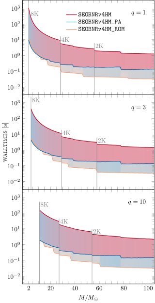
The SEOBNRv4HM_PA model was benchmarked against other relevant waveform models which are available in LALSimulation: against SEOBNRv4HM (Cotesta et al., 2018), SEOBNRv4HM_ROM (Cotesta, Roberto and Marsat, Sylvain and Pürrer, Michael, 2020)  and SEOBNRv4T_surrogate (Lackey, Benjamin D. and Pürrer, Michael and Taracchini, Andrea and Marsat, Sylvain, 2019) in computational efficiency, and against SEOBNRv4HM in accuracy. Figure 1 shows the time for generating a waveform for total masses between 2 and $100M_{\odot}$, with starting frequency of $10\text{\,}\mathrm{Hz}$, and for three values of the mass ratio, $q=\{1,3,10\}$. The SEOBNRv4HM_PA model performs significantly faster than the SEOBNRv4HM model across all values of the total mass $M$. The speedup is most significant for lower total mass ($\sim 60\times$), and drops to its lowest for high total mass ($\sim 10\times$). Most importantly, the speedup is substantial ($\sim 30\times$) for $M\sim 40-60M_{\odot}$, where many of the events of current interest lie. For $M\gtrsim 10M_{\odot}$, the time to generate a waveform using SEOBNRv4HM_PA is less than 1 s.

Comparing to the frequency-domain SEOBNRv4HM_ROM model, we see that, as expected, the reduced order model is faster in almost all cases, except for very low total mass ($M\lesssim 10M_{\odot}$) where the two models are comparable in terms of computational cost (see Fig. 1).

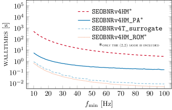
As a further test, the SEOBNRv4HM_PA model was benchmarked against the SEOBNRv4T_surrogate model, which only includes the $(\ell,|m|)=(2,2)$ mode. Figure 2 compares the time for generation of a waveform with the SEOBNRv4HM_PA and SEOBNRv4T_surrogate models where only the quadrupole mode is computed, at different sampling rates, and with different starting frequencies, for a $1.4M_{\odot}+1.4M_{\odot}$ bns with no spins.

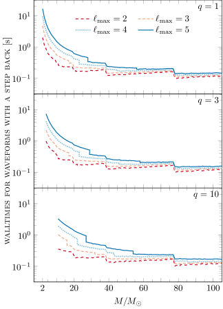
Finally, we benchmark the time necessary to generate each higher-oder multipole of the model. Figure 3 shows the times to generate waveforms with the SEOBNRv4HM_PA model for which all $(\ell,|m|)$ modes with $\ell\leq\ell_{\mathrm{max}}$ (see the legend) are resolved at initial frequency of $f_{0}=$20\text{\,}\mathrm{Hz}$$. As expected, adding higher multipoles increases the Nyquist frequency and the cost for generating the waveform. The figure demonstrates the difference in time that it takes to compute each of the modes of the model. Another test demonstrated that generating additional, higher-order modes at a fixed sampling rate incurs negligible computational cost to the waveform generation.

III.2 Accuracy of the model

To assess the accuracy of our model with respect to SEOBNRv4HM we use the notion of unfaithfulness as outlined below.

In general, the gw signal from a non-precessing, quasi-circular bbh is characterized by a total of 11 parameters: the binary companion masses $m_{1}$ and $m_{2}$, the (dimensionless) component spins $\chi_{1}$ and $\chi_{2}$, which can be aligned or anti-aligned with the orbital angular momentum, the orientation of the binary in the source frame $(\iota,\varphi_{0})$, the sky location of the source in the detector frame $(\theta,\phi)$, and the luminosity distance $d_{L}$, the time of arrival $t_{c}$, and the polarization angle $\psi$. The detector response can be written as

$$h(t) =F_{+}(\theta,\phi,\psi)\,h_{+}(\bm{\lambda},t_{c};t)+F_{\times}(\theta,\phi,\psi)\,h_{\times}(\bm{\lambda},t_{c};t),$$ (13)

where $\bm{\lambda}=(m_{1},m_{2},\chi_{1},\chi_{2},\iota,\varphi_{0},d_{L})$ are the binary parameters and the functions $F_{\{+,\times\}}(\theta,\phi,\psi)$ are the antenna patterns (see (Sathyaprakash and Dhurandhar, 1991; Finn and Chernoff, 1993)). This can be cast as

$$h(t) =\mathcal{A}(\theta,\phi)\big{(}\cos(\kappa)\,h_{+}(\bm{\lambda},t_{c};t)+\sin(\kappa)\,h_{\times}(\bm{\lambda},t_{c};t)\big{)}.$$ (14)

Here $\kappa\equiv\kappa(\theta,\phi,\psi)$ is the effective polarization (Capano et al., 2014), defined as

$$\exp(i\kappa(\theta,\phi,\psi))=\frac{F_{+}(\theta,\phi,\psi)+iF_{\times}(\theta,\phi,\psi)}{\mathcal{A}(\theta,\phi)},$$ (15)

where the overall amplitude function $\mathcal{A}(\theta,\phi)$ is

$$\mathcal{A}(\theta,\phi)=\sqrt{F_{+}^{2}(\theta,\phi,\psi)+F_{\times}^{2}(\theta,\phi,\psi)}\;.$$ (16)

We can now define the match between a gw signal $h_{\mathrm{\textsc{s}}}(t)$ (which for us is SEOBNRv4HM) and a template waveform $h_{\mathrm{\textsc{t}}}(t)$ (which is SEOBNRv4HM_PA) (see (Harry et al., 2016)):

$$\mathcal{F}(\iota_{\mathrm{\textsc{s}}},{\varphi_{0}}_{\mathrm{\textsc{s}}},\kappa_{\mathrm{\textsc{s}}})=\max_{t_{c},{\varphi_{0}}_{\mathrm{\textsc{t}}},\kappa_{\mathrm{\textsc{t}}}}\left[\left.\frac{(h_{\mathrm{\textsc{s}}},h_{\mathrm{\textsc{t}}})}{\sqrt{(h_{\mathrm{\textsc{s}}},h_{\mathrm{\textsc{s}}})(h_{\mathrm{\textsc{t}}},h_{\mathrm{\textsc{t}}})}}\right|_{\begin{subarray}{c}{m_{1,2}}_{\mathrm{\textsc{s}}}={m_{1,2}}_{\mathrm{\textsc{t}}}\\ {\chi_{1,2}}_{\mathrm{\textsc{s}}}={\chi_{1,2}}_{\mathrm{\textsc{t}}}\\ {\iota_{\mathrm{\textsc{s}}}=\iota_{\mathrm{\textsc{t}}}}\end{subarray}}\right],$$ (17)

where the parameters denoted with s (t) refer to the signal (template) waveform. For the purposes of this calculation, we marginalize over the phase ${\phi_{0}}_{\mathrm{\textsc{t}}}$, the effective polarization $\kappa_{\mathrm{\textsc{t}}}$, and the time of arrival $t_{c}$, and use the familiar definition for the inner product between two waveforms (Sathyaprakash and Dhurandhar, 1991; Finn and Chernoff, 1993):

$$(x,y)\equiv 4\;\Re\left[\int_{f_{\mathrm{low}}}^{f_{\mathrm{high}}}\mathrm{d}f\;\frac{\widetilde{x}(f)\;\widetilde{y}^{*}(f)}{S_{\mathrm{n}}(f)}\right],$$ (18)

where a $\sim$ denotes a Fourier transform, a $*$ denotes a complex conjugate, and finally $S_{\mathrm{n}}(f)$ is the one-sided power spectral density (psd) of the detector noise.

Here, we use $f_{\mathrm{low}}=$20\text{\,}\mathrm{Hz}$$, $f_{\mathrm{high}}=$2048\text{\,}\mathrm{Hz}$$, and the Advanced ligo ”zero-tuned high-power” design sensitivity curve (Barsotti et al., 2018). The definition of the faithfulness in Eq. (17) depends on the signal parameters ($\iota_{\mathrm{\textsc{s}}},{\varphi_{0}}_{\mathrm{\textsc{s}}},\kappa_{\mathrm{\textsc{s}}}$) and therefore allows us to work with either the maximum or the averaged unfaithfulness (or mismatch) $1-\mathcal{F}(\iota_{\mathrm{\textsc{s}}},{\varphi_{0}}_{\mathrm{\textsc{s}}},\kappa_{\mathrm{\textsc{s}}})$:

$$\mathcal{U}_{\mathrm{max}} \equiv\max_{\{\iota_{\mathrm{\textsc{s}}},{\varphi_{0}}_{\mathrm{\textsc{s}}},\kappa_{\mathrm{\textsc{s}}}\}}\left[1-\mathcal{F}\right]\equiv 1-\min_{\{\iota_{\mathrm{\textsc{s}}},{\varphi_{0}}_{\mathrm{\textsc{s}}},\kappa_{\mathrm{\textsc{s}}}\}}\left[\mathcal{F}\right],$$ (19a)

$$\mkern 1.5mu\overline{\mkern-1.5mu\mathcal{U}\mkern-1.5mu}\mkern 1.5mu \equiv\langle 1-\mathcal{F}\rangle_{\{\iota_{\mathrm{\textsc{s}}},{\varphi_{0}}_{\mathrm{\textsc{s}}},\kappa_{\mathrm{\textsc{s}}}\}}\equiv 1-\frac{1}{8\pi^{2}}\int_{0}^{2\pi}\mathrm{d}\kappa_{\mathrm{\textsc{s}}}\int_{0}^{\pi}\mathrm{d}\iota_{\mathrm{\textsc{s}}}\sin(\iota_{\mathrm{\textsc{s}}})\int_{0}^{2\pi}\mathrm{d}{\varphi_{0}}_{\mathrm{\textsc{s}}}\mathcal{F}.$$ (19b)

Fig. 5: Histogram of the unfaithfulness $\,\mkern 1.5mu\overline{\mkern-1.5mu\mathcal{U}\mkern-1.5mu}\mkern 1.5mu$ (in percent) between the SEOBNRv4HM_PA and SEOBNRv4HM models for 4 different values of the total mass $M$.

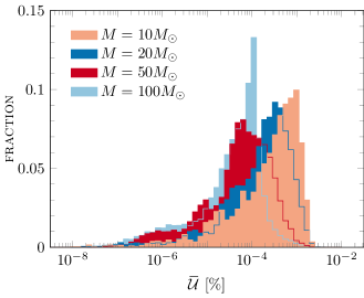
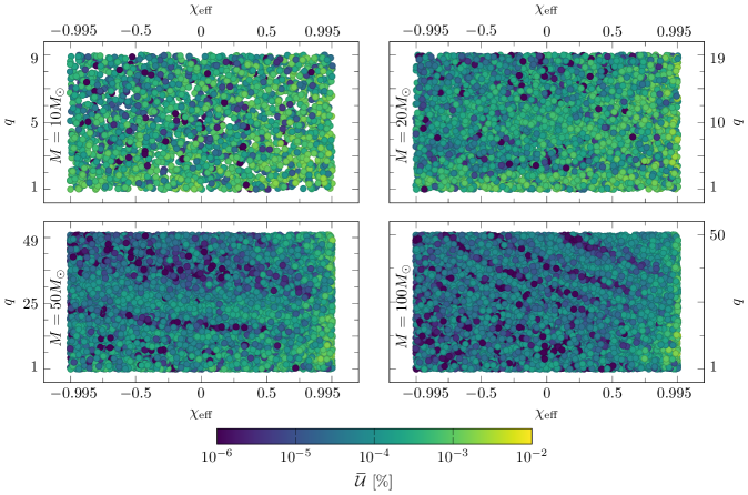
Using these definitions of the unfaithfulness, we examine the accuracy of the post-adiabatic (pa) model in comparison with SEOBNRv4HM. Figure 4 shows the maximum unfaithfulness $\mathcal{U}_{\mathrm{max}}$ across the parameter space of the effective spin $\chi_{\mathrm{eff}}$ and the mass ratio $q$ for 4 separate values of the total mass $M$. We find that in all cases that were presented, the unfaithfulness is below $\mathcal{O}(0.01\%)$, which makes our model comparable in accuracy to SEOBNRv4HM_ROM (Cotesta, Roberto and Marsat, Sylvain and Pürrer, Michael, 2020). The variations of the unfaithfulness for a fixed total mass can be explained in terms of the length of the waveform and the heuristic condition which we use to transition from pa inspiral to merger and ringdown.

The variations across the separate panels of Fig. 4 can be better expressed in the form of a histogram of the average unfaithfulness $\mkern 1.5mu\overline{\mkern-1.5mu\mathcal{U}\mkern-1.5mu}\mkern 1.5mu$, which is shown in Fig. 5. The distribution for each value of the total mass $M$ peaks at a higher value of the unfaithfulness, which is consistent with the fact that lower-mass binaries undergo a longer coalescence inside the frequency band relevant to ligo. In all cases, however, the average unfaithfulness stays below $\mathcal{O}(0.01\%)$.

(a) Marginalized 2D posterior for the component source-frame masses $m_{1}$ and $m_{2}$.

(b) Marginalized 2D posterior for the mass ratio $q$ and the effective spin $\chi_{\mathrm{eff}}$.

(c) Marginalized 2D posterior for the luminosity distance $d_{L}$ and the inclination of the binary $\theta$.

Fig. 6: Parameter estimation results for the synthetic injection. The 2-dimensional posterior plots show the 90% confidence regions for the parameters. The grey vertical lines in the 1-dimensional plots show the projections of these confidence regions. The grey labelled lines denote the injection values. Note the excellent agreement between SEOBNRv4HM_PA and SEOBNRv4HM waveform models.

IV Parameter estimation study

While the previous section deals with the absolute performance of the SEOBNRv4HM_PA model, it is important to demonstrate that these benchmarks translate into a faster and reliable parameter estimation (pe) analyses. For this purpose, two pe studies were performed with the SEOBNRv4HM_PA model, as well as some of the established waveform models (SEOBNRv4HM or SEOBNRv4HM_ROM). The first one is an injection study involving a synthetic signal. The data is then analysed using SEOBNRv4HM_PA and SEOBNRv4HM models. The second pe study was performed on data from the event GW190412. It was analysed using the SEOBNRv4HM_PA and the SEOBNRv4HM_ROM models.

In both cases, the parameter estimation was done using the Markov-chain Monte Carlo code LALinferenceMCMC (ligo Scientific Collaboration, 2018). The results of these studies are presented below in the following subsections. We also note that pe studies using the TEOBResumS waveform model with the pa approximation were done in Refs (Akcay et al., 2019; Gamba et al., 2020a; Akcay et al., 2021; Gamba et al., 2020b; Breschi et al., 2021).

IV.1 Injection-based study

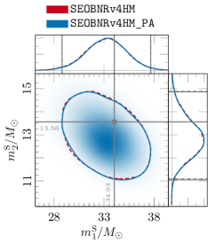
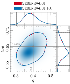
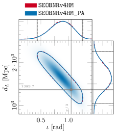
The choice of parameters for this pe study was made so that it could emphasise the speedup which the SEOBNRv4HM_PA model offers, but also to manifest higher-order modes in the signal. The injected signal has total mass $M=60M_{\odot}$ with mass ratio $1/q\approx 0.4$, aligned spins $(\chi_{1},\chi_{2})=(0.8,0.3)$, at a distance of approximately 1364 Mpc (corresponding to signal-to-noise ratio (snr) of $\sim 22$) and at an inclination of $\pi/3$. The injection was made using the SEOBNRv4HM model, while the subsequent analysis was performed using both the SEOBNRv4HM and the SEOBNRv4HM_PA models in order to judge the performance of the post-adiabatic (pa) model.

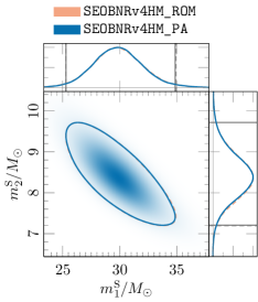
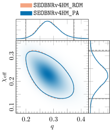
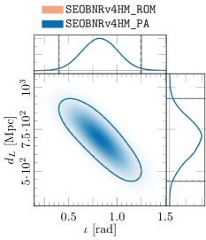
The results of the parameter estimation analysis can be summarized in the series of marginalized 2-dimensional posterior plots in Fig. 6. Figure 6a shows the plot for the component source-frame masses $m_{1}^{\textsc{s}}$ and $m_{2}^{\textsc{s}}$; Fig. 6b shows the plot for the mass ratio $q$ and the effective spin $\chi_{\mathrm{eff}}$. Finally, Fig. 6c shows the posterior for the luminosity distance $d_{L}$ (cf. Eq. (11)) and the inclination angle $\iota$. The plots demonstrate that the distributions of the posterior samples are in very good agreement between the two models, which demonstrates the reliability of SEOBNRv4HM_PA in pe studies. The Jensen-Shannon (js) divergence between the 1-dimensional posteriors which are shown in Fig. 6 is always at $\mathcal{O}\!\left(10^{-3}\right)$ or below, which is consistent with the effects of stochastic sampling on the recovered quantities (Romero-Shaw et al., 2020).

(a) Marginalized 2D posterior for the component source-frame masses $m_{1}$ and $m_{2}$.

(b) Marginalized 2D posterior for the mass ratio $q$ and the effective spin $\chi_{\mathrm{eff}}$.

(c) Marginalized 2D posterior for the luminosity distance $d_{L}$ and the inclination of the binary $\iota$.

Fig. 7: Parameter estimation results for the event GW190412. The 2-dimensional posterior plots show the 90% confidence regions for the parameters. The grey vertical lines in the 1-dimensional plots show the projections of these confidence regions. There is an excellent agreement between the results with the SEOBNRv4HM_PA and the SEOBNRv4HM_ROM models.

IV.2 GW190412 parameter estimation

It is more interesting to demonstrate the viability of the SEOBNRv4HM_PA model on a real gw-event. The GW190412 from the LIGO O3a catalogue is a good candidate for such a study due to its parameters – total mass of $\lesssim 40M_{\odot}$ ($m_{1}\approx 30M_{\odot}$ and $m_{2}\approx 8M_{\odot}$, asymmetric mass ratio of about 3, and dimensionless spin of the massive companion between 0.22 and 0.6 (Abbott et al., 2020b; Zevin et al., 2020; Islam et al., 2020; Colleoni et al., 2021). The total mass and mass ratio suggest that waveforms for this event would be computationally much more efficient using the SEOBNRv4HM_PA model – which means it is particularly suitable to study this event. The analyses were performed with both the SEOBNRv4HM_PA and SEOBNRv4HM_ROM models, since any analysis with the SEOBNRv4HM model would have been impractical in terms of the time required to complete it.

The 2-dimensional marginalized posterior plots are shown in Fig. 7. Figure 7a shows the posterior for the component source-frame masses $m_{1}^{\textsc{s}}$ and $m_{2}^{\textsc{s}}$ of the binary; Fig. 7b shows the plot for the mass ratio $q$ and the effective spin $\chi_{\mathrm{eff}}$; and finally, Fig. 7c shows the plot for the luminosity distance $d_{L}$ and the inclination angle $\iota$. The plots demonstrate the incredibly good agreement between the SEOBNRv4HM_ROM and the SEOBNRv4HM_PA models, which is further confirmed by the js divergence between the samples, which is below the $\mathcal{O}\!\left(10^{-3}\right)$ level.

In conclusion for this section, the SEOBNRv4HM_PA model may be reliably used for parameter estimation analyses in place of models like SEOBNRv4HM, with no evident caveats which could hinder the results of such analyses. Furthermore, the average speedup in the generation of samples for the mcmc chains was found to be around 1 order of magnitude. The reason that this is less compared to the speedup demonstrated in Fig. 1 is the fact that for the pe studies, the waveforms are generated using starting frequency $f_{0}=$20\text{\,}\mathrm{Hz}$$.

V Tests of General Relativity

In previous sections we have seen that SEOBNRv4HM_PA is a robust, accurate and fast alternative to SEOBNRv4HM and can therefore be used as a drop-in replacement. An interesting further application of this is to use the SEOBNRv4HM_PA model for tests of General Relativity, where the SEOBNRv4HM model was previously used as a baseline gr model. In particular, we consider a parametrized black hole (bh) ringdown test that measures the deviations of quasi-normal mode emission from predictions of gr. We summarize the test briefly here, see (Abbott et al., 2020h; Ghosh et al., 2021) for more details. In gr, the no-hair conjecture predicts that the physical properties of a (uncharged) bh are completely determined by its mass and spin. Consequently, the quasi-normal modes (qnm) that describe the gravitational waves emitted by a perturbed bh are also uniquely determined by its mass and spin. Thus one can check the validity of gr by measuring or constraining any deviations in the complex qnm frequencies. The pSEOBNR ringdown analysis uses a parameterised version of a full inspiral-merger-ringdown gw signal model to measure and constrain the (complex) qnm frequencies. Consequently, unlike other ringdown studies restricted to the post-merger signal (Isi et al., 2019; Giesler et al., 2019; Carullo et al., 2019a, b), the pSEOBNR analysis makes use of the entire signal power and does not suffer from the ambiguity of a ringdown start-time definition. In pSEOBNR, one starts with the SEOBNRv4HM model, but then introduces deviations $\delta f_{lm0}$ and $\delta\tau_{lm0}$ (which are treated as free parameters) to the qnm frequency and damping time, so that

$$f_{lm0} =f_{lm0}^{\rm\textsc{gr}}\left(1+\delta f_{lm0}\right),$$ (20)

$$\tau_{lm0} =\tau_{lm0}^{\rm\textsc{gr}}\left(1+\delta\tau_{lm0}\right),$$ (21)

and the ringdown signal is different from the gr prediction. Here, $f_{lm0}^{\rm\textsc{gr}}$ and $\tau_{lm0}^{\rm\textsc{gr}}$ are computed from final mass and spin as predicted by nr fitting formulae. The goal of the test is to infer the values of the $(\delta f_{lm0}$, $\delta\tau_{lm0})$ by doing full parameter estimation.

Fig. 8: Posterior distributions for the fractional deviations $\delta f_{220}$ and $\delta\tau_{220}$ in the damping time and frequency as recovered by using SEOBNRv4HM and SEOBNRv4HM_PA. The 2-dimensional posterior plot shows the 90% confidence regions for the parameters. The grey vertical lines in the 1-dimensional plots show the projections of these confidence regions. The thick grey lines denote the values predicted by gr.

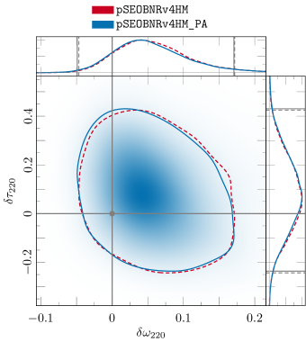
Performing full parameter estimation taking into account deviations from gr is a challenging problem, since it involves sampling a higher-dimensional space (two new parameters for every $(\ell,m)$ mode considered), which means any improvements to waveform speed can lead to even bigger impact on the overall runtime. To check the speed and accuracy of using SEOBNRv4HM_PA for this application, we compare it to the results obtained with SEOBNRv4HM for the first gravitational wave event ever detected, GW150914. We choose this event as it has significant signal-to-noise ratio (snr) in the merger-ringdown regime. For a high (quasi) equal-mass binary like GW150914, contributions from higher multipoles of the gw signal are expected to be negligible. Hence, we restrict our analysis to just the least-damped dominant qnm, i.e., $(f_{220},\tau_{220})$, keeping the other qnms fixed at their nominal gr values. In Fig. 8 we show the posterior distributions for the fractional deviations in the damping time and frequency as recovered by using SEOBNRv4HM and SEOBNRv4HM_PA. It is evident that the posteriors are in extremely good agreement with the results showing consistency with gr. More quantitatively, the Jensen–Shannon (js) divergence between the 1-dimensional posteriors is $\mathcal{O}(10^{-3})$ for $\delta f_{220}$ and $\delta\tau_{220}$, which is again within the range of what is expected due to stochastic sampling. We find a similarly good level of agreement for the other parameters. Finally, we find a speed-up of $\sim 10$ times when using SEOBNRv4HM_PA instead of SEOBNRv4HM as the base gr model, significantly accelerating inference. With focus shifting from analyses of individual events to population studies, demands on computational resources and person-power are ever-increasing, as demonstrated by large-scale studies in lvk catalog papers (Abbott et al., 2019; Nitz et al., 2020). Hence, such increases in computational efficiency is immensely important for the future of gw data analysis.

VI Discussion and conclusions

We developed the SEOBNRv4HM_PA model, which combines the multipolar eob nr-informed model SEOBNRv4HM with the post-adiabatic (pa) approach for solving the (spin-aligned) binary dynamics (developed and used in the TEOBResumS models (Damour et al., 2013; Nagar and Rettegno, 2019; Rettegno et al., 2020; Riemenschneider et al., 2021)). The resulting model is computationally cheap (at most on the order of seconds and less than 1 second for most of the parameter space) and highly accurate (unfaithfulness less than $\mathcal{O}(10^{-3})$ when benchmarked against the SEOBNRv4HM model). Therefore, it can be used as a drop-in replacement for parameter estimation studies and tests of gr for many gw events where the use of the SEOBNRv4HM model would have been impractical.

In Sec. II we presented the eob formalism and the derivation of the pa equations, together with a discussion on the specifics of transitioning from the pa regime to the merger part of the dynamics. Section III describes the practical implementation of this model in the LALSimulation library of waveform models, and provides the important benchmarks in terms of speed and accuracy of the SEOBNRv4HM_PA model. In particular, we demonstrated that the SEOBNRv4HM_PA model provides a speed-up of 10 to 100 times compared to the SEOBNRv4HM waveform model. Furthermore, we showed that the new model is accurate at a level which allows us to use it for the purposes of ligo data analysis.

Section IV makes use of the results of the previous section and illustrates the use of the SEOBNRv4HM_PA model in 2 separate parameter estimation studies: recovering an injected synthetic signal and applying the model to analyse the event GW190412. In both cases, we find an extremely good agreement between the results obtained with our model and other established models. Compared to pe with the SEOBNRv4HM model, the study with SEOBNRv4HM_PA completes around 10 times faster. Finally, Sec. V depicts the use of the waveform model to a test of gr and discusses the importance of the model for this type of analyses. We find that there is an excellent agreement between the results obtained using the SEOBNRv4HM_PA and the established SEOBNRv4HM and SEOBNRv4HM_ROM models.

There are several interesting future directions that can be pursued to apply the pa approximation to other SEOBNRv4HM models, notably models that include tidal deformabilities for binary neutron stars (Hinderer et al., 2016; Steinhoff et al., 2016), for which, currently, only the surrogate method has been applied (Lackey, Benjamin D. and Pürrer, Michael and Taracchini, Andrea and Marsat, Sylvain, 2019) (see Refs. (Akcay et al., 2019; Nagar et al., 2019) for pa models with tidal effects using TEOBResumS). A more important but challenging extension would involve the precessing SEOBNRv4PHM Hamiltonian (Ossokine et al., 2020), which would allow the model to be used more efficiently and for a broader range of gw events when doing parameter-estimation studies. Finally, the pa approximation could also be extended to binary systems on eccentric dynamics. The main challenges with spin-precession and eccentricity is the presence of time scales beyond the orbital and radiation-reaction ones.

References

- Abbott et al. (2016a) B. P. Abbott et al. (Virgo, LIGO Scientific), Phys. Rev. Lett. 116, 061102 (2016a), arXiv:1602.03837 [gr-qc].
- Abbott et al. (2016b) B. P. Abbott et al. (LIGO Scientific, Virgo), Phys. Rev. X6, 041015 (2016b), [Erratum: Phys. Rev. X8, no. 3, 039903 (2018)], arXiv:1606.04856 [gr-qc].
- Venumadhav et al. (2020) T. Venumadhav, B. Zackay, J. Roulet, L. Dai, and M. Zaldarriaga, Phys. Rev. D 101, 083030 (2020), arXiv:1904.07214 [astro-ph.HE].
- Nitz et al. (2019) A. H. Nitz, C. Capano, A. B. Nielsen, S. Reyes, R. White, D. A. Brown, and B. Krishnan, Astrophys. J. 872, 195 (2019), arXiv:1811.01921 [gr-qc].
- Nitz et al. (2020) A. H. Nitz, T. Dent, G. S. Davies, S. Kumar, C. D. Capano, I. Harry, S. Mozzon, L. Nuttall, A. Lundgren, and M. Tápai, Astrophys. J. 891, 123 (2020), arXiv:1910.05331 [astro-ph.HE].
- Zackay et al. (2019) B. Zackay, L. Dai, T. Venumadhav, J. Roulet, and M. Zaldarriaga, arXiv e-prints , arXiv:1910.09528 (2019), arXiv:1910.09528 [astro-ph.HE].
- Abbott et al. (2019) B. P. Abbott et al. (LIGO Scientific, Virgo), Phys. Rev. X9, 031040 (2019), arXiv:1811.12907 [astro-ph.HE].
- Abbott et al. (2020a) R. Abbott et al. (LIGO Scientific, Virgo), (2020a), arXiv:2010.14527 [gr-qc].
- Aasi et al. (2015) J. Aasi et al. (LIGO Scientific), Class. Quant. Grav. 32, 074001 (2015), arXiv:1411.4547 [gr-qc].
- Acernese et al. (2015) F. Acernese et al. (VIRGO), Class. Quant. Grav. 32, 024001 (2015), arXiv:1408.3978 [gr-qc].
- (11) “, Information about gravitational-wave detections made by ligo to date,” https://www.ligo.org/detections.php, accessed: March 7, 2021.
- Abbott et al. (2020b) R. Abbott et al. (LIGO Scientific, Virgo), Phys. Rev. D 102, 043015 (2020b), arXiv:2004.08342 [astro-ph.HE].
- Abbott et al. (2020c) R. Abbott et al. (LIGO Scientific, Virgo), Astrophys. J. Lett. 896, L44 (2020c), arXiv:2006.12611 [astro-ph.HE].
- Abbott et al. (2020d) R. Abbott et al. (LIGO Scientific, Virgo), Phys. Rev. Lett. 125, 101102 (2020d), arXiv:2009.01075 [gr-qc].
- Dominik et al. (2015) M. Dominik, E. Berti, R. O’Shaughnessy, I. Mandel, K. Belczynski, C. Fryer, D. E. Holz, T. Bulik, and F. Pannarale, Astrophys. J. 806, 263 (2015), arXiv:1405.7016 [astro-ph.HE].
- Belczynski et al. (2016) K. Belczynski, S. Repetto, D. E. Holz, R. O’Shaughnessy, T. Bulik, E. Berti, C. Fryer, and M. Dominik, Astrophys. J. 819, 108 (2016), arXiv:1510.04615 [astro-ph.HE].
- Abbott et al. (2020e) B. P. Abbott et al. (KAGRA, LIGO Scientific, Virgo), Living Rev. Rel. 23, 3 (2020e).
- Punturo et al. (2010) M. Punturo et al., Class. Quant. Grav. 27, 194002 (2010).
- Reitze et al. (2019) D. Reitze et al., Bull. Am. Astron. Soc. 51, 035 (2019), arXiv:1907.04833 [astro-ph.IM].
- Amaro-Seoane et al. (2017) P. Amaro-Seoane et al. (LISA), (2017), arXiv:1702.00786 [astro-ph.IM].
- Buonanno and Sathyaprakash (2014) A. Buonanno and B. S. Sathyaprakash, “A. Buonanno, Sources of Gravitational Waves: Theory and Observations,” (2014) arXiv:1410.7832 [gr-qc].
- Abbott et al. (2020f) B. P. Abbott et al. (LIGO Scientific, Virgo), Class. Quant. Grav. 37, 055002 (2020f), arXiv:1908.11170 [gr-qc].
- Harry et al. (2009) I. W. Harry, B. Allen, and B. S. Sathyaprakash, Phys. Rev. D 80, 104014 (2009), arXiv:0908.2090 [gr-qc].
- Veitch et al. (2015) J. Veitch et al., Phys. Rev. D 91, 042003 (2015), arXiv:1409.7215 [gr-qc].
- Cutler et al. (1993) C. Cutler et al., Phys. Rev. Lett. 70, 2984 (1993), arXiv:astro-ph/9208005.
- Lindblom et al. (2008) L. Lindblom, B. J. Owen, and D. A. Brown, Phys. Rev. D78, 124020 (2008), arXiv:0809.3844 [gr-qc].
- Pürrer and Haster (2020) M. Pürrer and C.-J. Haster, Phys. Rev. Res. 2, 023151 (2020), arXiv:1912.10055 [gr-qc].
- Abbott et al. (2020g) R. Abbott et al. (LIGO Scientific, Virgo), (2020g), arXiv:2010.14533 [astro-ph.HE].
- Abbott et al. (2020h) R. Abbott et al. (LIGO Scientific, Virgo), (2020h), arXiv:2010.14529 [gr-qc].
- Buonanno and Damour (1999) A. Buonanno and T. Damour, Phys.Rev. D59, 084006 (1999), arXiv:gr-qc/9811091 [gr-qc].
- Buonanno and Damour (2000) A. Buonanno and T. Damour, Phys. Rev. D62, 064015 (2000), arXiv:gr-qc/0001013 [gr-qc].
- Damour et al. (2000) T. Damour, P. Jaranowski, and G. Schaefer, Phys. Rev. D62, 084011 (2000), arXiv:gr-qc/0005034 [gr-qc].
- Damour (2001) T. Damour, Phys. Rev. D64, 124013 (2001), arXiv:gr-qc/0103018 [gr-qc].
- Buonanno et al. (2006) A. Buonanno, Y. Chen, and T. Damour, Phys. Rev. D 74, 104005 (2006), arXiv:gr-qc/0508067.
- Buonanno et al. (2007) A. Buonanno, G. B. Cook, and F. Pretorius, Phys. Rev. D 75, 124018 (2007), arXiv:gr-qc/0610122.
- Damour et al. (2009) T. Damour, B. R. Iyer, and A. Nagar, Phys. Rev. D79, 064004 (2009), arXiv:0811.2069 [gr-qc].
- Pan et al. (2011a) Y. Pan, A. Buonanno, R. Fujita, E. Racine, and H. Tagoshi, Phys. Rev. D 83, 064003 (2011a), [Erratum: Phys. Rev. D 87, 109901 (2013)], arXiv:1006.0431 [gr-qc].
- Pan et al. (2011b) Y. Pan, A. Buonanno, M. Boyle, L. T. Buchman, L. E. Kidder, H. P. Pfeiffer, and M. A. Scheel, Phys. Rev. D 84, 124052 (2011b), arXiv:1106.1021 [gr-qc].
- Barausse and Buonanno (2010) E. Barausse and A. Buonanno, Phys. Rev. D 81, 084024 (2010), arXiv:0912.3517 [gr-qc].
- Taracchini et al. (2012) A. Taracchini, Y. Pan, A. Buonanno, E. Barausse, M. Boyle, T. Chu, G. Lovelace, H. P. Pfeiffer, and M. A. Scheel, Phys. Rev. D86, 024011 (2012), arXiv:1202.0790 [gr-qc].
- Taracchini et al. (2014) A. Taracchini et al., Phys. Rev. D89, 061502 (2014), arXiv:1311.2544 [gr-qc].
- Pan et al. (2014) Y. Pan, A. Buonanno, A. Taracchini, L. E. Kidder, A. H. Mroué, H. P. Pfeiffer, M. A. Scheel, and B. Szilágyi, Phys. Rev. D89, 084006 (2014), arXiv:1307.6232 [gr-qc].
- Bohé et al. (2017) A. Bohé, L. Shao, A. Taracchini, A. Buonanno, S. Babak, I. W. Harry, I. Hinder, S. Ossokine, M. Pürrer, V. Raymond, and et al., Phys. Rev. D 95, 044028 (2017), arXiv:1611.03703 [gr-qc].
- Babak et al. (2017) S. Babak, A. Taracchini, and A. Buonanno, Phys. Rev. D95, 024010 (2017), arXiv:1607.05661 [gr-qc].
- Cotesta et al. (2018) R. Cotesta, A. Buonanno, A. Bohé, A. Taracchini, I. Hinder, and S. Ossokine, Phys. Rev. D98, 084028 (2018), arXiv:1803.10701 [gr-qc].
- Ossokine et al. (2020) S. Ossokine et al., Phys. Rev. D 102, 044055 (2020), arXiv:2004.09442 [gr-qc].
- Damour and Nagar (2014) T. Damour and A. Nagar, Phys. Rev. D90, 044018 (2014), arXiv:1406.6913 [gr-qc].
- Nagar et al. (2016) A. Nagar, T. Damour, C. Reisswig, and D. Pollney, Phys. Rev. D93, 044046 (2016), arXiv:1506.08457 [gr-qc].
- Nagar et al. (2018) A. Nagar et al., Phys. Rev. D 98, 104052 (2018), arXiv:1806.01772 [gr-qc].
- Nagar et al. (2021) A. Nagar, A. Bonino, and P. Rettegno, (2021), arXiv:2101.08624 [gr-qc].
- Ajith et al. (2011) P. Ajith et al., Phys. Rev. Lett. 106, 241101 (2011), arXiv:0909.2867 [gr-qc].
- Santamaria et al. (2010) L. Santamaria et al., Phys. Rev. D82, 064016 (2010), arXiv:1005.3306 [gr-qc].
- Hannam et al. (2014) M. Hannam, P. Schmidt, A. Bohé, L. Haegel, S. Husa, F. Ohme, G. Pratten, and M. Pürrer, Phys. Rev. Lett. 113, 151101 (2014), arXiv:1308.3271 [gr-qc].
- Husa, Sascha and Khan, Sebastian and Hannam, Mark and Pürrer, Michael and Ohme, Frank and Jiménez Forteza, Xisco and Bohé, Alejandro (2016) Husa, Sascha and Khan, Sebastian and Hannam, Mark and Pürrer, Michael and Ohme, Frank and Jiménez Forteza, Xisco and Bohé, Alejandro, Phys. Rev. D 93, 044006 (2016), arXiv:1508.07250 [gr-qc].
- Khan et al. (2016) S. Khan, S. Husa, M. Hannam, F. Ohme, M. Pürrer, X. Jiménez Forteza, and A. Bohé, Phys. Rev. D93, 044007 (2016), arXiv:1508.07253 [gr-qc].
- London et al. (2018) L. London, S. Khan, E. Fauchon-Jones, C. García, M. Hannam, S. Husa, X. Jiménez-Forteza, C. Kalaghatgi, F. Ohme, and F. Pannarale, Phys. Rev. Lett. 120, 161102 (2018), arXiv:1708.00404 [gr-qc].
- Khan et al. (2019) S. Khan, K. Chatziioannou, M. Hannam, and F. Ohme, Phys. Rev. D100, 024059 (2019), arXiv:1809.10113 [gr-qc].
- Khan et al. (2020) S. Khan, F. Ohme, K. Chatziioannou, and M. Hannam, Phys. Rev. D101, 024056 (2020), arXiv:1911.06050 [gr-qc].
- Pratten et al. (2020) G. Pratten, S. Husa, C. Garcia-Quiros, M. Colleoni, A. Ramos-Buades, H. Estelles, and R. Jaume, Phys. Rev. D 102, 064001 (2020), arXiv:2001.11412 [gr-qc].
- Pretorius (2005) F. Pretorius, Phys. Rev. Lett. 95, 121101 (2005), arXiv:gr-qc/0507014 [gr-qc].
- Campanelli et al. (2006) M. Campanelli, C. O. Lousto, P. Marronetti, and Y. Zlochower, Phys. Rev. Lett. 96, 111101 (2006), arXiv:gr-qc/0511048 [gr-qc].
- Baker et al. (2006) J. G. Baker, J. Centrella, D.-I. Choi, M. Koppitz, and J. van Meter, Phys. Rev. Lett. 96, 111102 (2006), arXiv:gr-qc/0511103 [gr-qc].
- Bruegmann et al. (2008) B. Bruegmann, J. A. Gonzalez, M. Hannam, S. Husa, U. Sperhake, and W. Tichy, Phys. Rev. D 77, 024027 (2008), arXiv:gr-qc/0610128.
- Centrella et al. (2010) J. Centrella, J. G. Baker, B. J. Kelly, and J. R. van Meter, Rev. Mod. Phys. 82, 3069 (2010), arXiv:1010.5260 [gr-qc].
- Mroue et al. (2013) A. H. Mroue et al., Phys. Rev. Lett. 111, 241104 (2013), arXiv:1304.6077 [gr-qc].
- Jani et al. (2016) K. Jani, J. Healy, J. A. Clark, L. London, P. Laguna, and D. Shoemaker, Class. Quant. Grav. 33, 204001 (2016), arXiv:1605.03204 [gr-qc].
- Healy et al. (2017) J. Healy, C. O. Lousto, Y. Zlochower, and M. Campanelli, Class. Quant. Grav. 34, 224001 (2017), arXiv:1703.03423 [gr-qc].
- Boyle et al. (2019) M. Boyle et al., Class. Quant. Grav. 36, 195006 (2019), arXiv:1904.04831 [gr-qc].
- Lange et al. (2018) J. Lange, R. O’Shaughnessy, and M. Rizzo, (2018), arXiv:1805.10457 [gr-qc].
- Nagar and Rettegno (2019) A. Nagar and P. Rettegno, Phys. Rev. D 99, 021501 (2019), arXiv:1805.03891 [gr-qc].
- Rettegno et al. (2020) P. Rettegno, F. Martinetti, A. Nagar, D. Bini, G. Riemenschneider, and T. Damour, Phys. Rev. D 101, 104027 (2020), arXiv:1911.10818 [gr-qc].
- Field et al. (2014) S. E. Field, C. R. Galley, J. S. Hesthaven, J. Kaye, and M. Tiglio, Phys. Rev. X 4, 031006 (2014), arXiv:1308.3565 [gr-qc].
- Pürrer (2014) M. Pürrer, Class. Quant. Grav. 31, 195010 (2014), arXiv:1402.4146 [gr-qc].
- Blackman et al. (2015) J. Blackman, S. E. Field, C. R. Galley, B. Szilágyi, M. A. Scheel, M. Tiglio, and D. A. Hemberger, Phys. Rev. Lett. 115, 121102 (2015), arXiv:1502.07758 [gr-qc].
- Pürrer (2016) M. Pürrer, Phys. Rev. D93, 064041 (2016), arXiv:1512.02248 [gr-qc].
- Blackman et al. (2017a) J. Blackman, S. E. Field, M. A. Scheel, C. R. Galley, D. A. Hemberger, P. Schmidt, and R. Smith, Phys. Rev. D 95, 104023 (2017a), arXiv:1701.00550 [gr-qc].
- Doctor, Zoheyr and Farr, Ben and Holz, Daniel E. and Pürrer, Michael (2017) Doctor, Zoheyr and Farr, Ben and Holz, Daniel E. and Pürrer, Michael, Phys. Rev. D 96, 123011 (2017), arXiv:1706.05408 [astro-ph.HE].
- Blackman et al. (2017b) J. Blackman, S. E. Field, M. A. Scheel, C. R. Galley, C. D. Ott, M. Boyle, L. E. Kidder, H. P. Pfeiffer, and B. Szilágyi, Phys. Rev. D96, 024058 (2017b), arXiv:1705.07089 [gr-qc].
- Lackey, Benjamin D. and Pürrer, Michael and Taracchini, Andrea and Marsat, Sylvain (2019) Lackey, Benjamin D. and Pürrer, Michael and Taracchini, Andrea and Marsat, Sylvain, Phys. Rev. D 100, 024002 (2019), arXiv:1812.08643 [gr-qc].
- Setyawati, Yoshinta and Pürrer, Michael and Ohme, Frank (2020) Setyawati, Yoshinta and Pürrer, Michael and Ohme, Frank, Class. Quant. Grav. 37, 075012 (2020), arXiv:1909.10986 [astro-ph.IM].
- Cotesta, Roberto and Marsat, Sylvain and Pürrer, Michael (2020) Cotesta, Roberto and Marsat, Sylvain and Pürrer, Michael, Phys. Rev. D 101, 124040 (2020), arXiv:2003.12079 [gr-qc].
- Varma et al. (2019a) V. Varma, S. E. Field, M. A. Scheel, J. Blackman, L. E. Kidder, and H. P. Pfeiffer, Phys. Rev. D99, 064045 (2019a), arXiv:1812.07865 [gr-qc].
- Varma et al. (2019b) V. Varma, S. E. Field, M. A. Scheel, J. Blackman, D. Gerosa, L. C. Stein, L. E. Kidder, and H. P. Pfeiffer, Phys. Rev. Research. 1, 033015 (2019b), arXiv:1905.09300 [gr-qc].
- Brown et al. (2013) D. A. Brown, P. Kumar, and A. H. Nitz, Phys. Rev. D 87, 082004 (2013), arXiv:1211.6184 [gr-qc].
- Capano et al. (2014) C. Capano, Y. Pan, and A. Buonanno, Phys. Rev. D89, 102003 (2014), arXiv:1311.1286 [gr-qc].
- Varma, Vijay and Ajith, Parameswaran and Husa, Sascha and Bustillo, Juan Calderon and Hannam, Mark and Pürrer, Michael (2014) Varma, Vijay and Ajith, Parameswaran and Husa, Sascha and Bustillo, Juan Calderon and Hannam, Mark and Pürrer, Michael, Phys. Rev. D 90, 124004 (2014), arXiv:1409.2349 [gr-qc].
- Varma and Ajith (2017) V. Varma and P. Ajith, Phys. Rev. D 96, 124024 (2017), arXiv:1612.05608 [gr-qc].
- Harry et al. (2018) I. Harry, J. Calderón Bustillo, and A. Nitz, Phys. Rev. D 97, 023004 (2018), arXiv:1709.09181 [gr-qc].
- Kalaghatgi et al. (2020) C. Kalaghatgi, M. Hannam, and V. Raymond, Phys. Rev. D 101, 103004 (2020), arXiv:1909.10010 [gr-qc].
- Damour et al. (2013) T. Damour, A. Nagar, and S. Bernuzzi, Phys. Rev. D 87, 084035 (2013), arXiv:1212.4357 [gr-qc].
- Riemenschneider et al. (2021) G. Riemenschneider, P. Rettegno, M. Breschi, A. Albertini, R. Gamba, S. Bernuzzi, and A. Nagar, (2021), arXiv:2104.07533 [gr-qc].
- Damour and Nagar (2008) T. Damour and A. Nagar, Phys. Rev. D 77, 024043 (2008), arXiv:0711.2628 [gr-qc].
- ligo Scientific Collaboration (2018) ligo Scientific Collaboration, “ligo Scientific Collaboration, ligo Algorithm Library – LALSuite,” free software (gpl) (2018).
- Burden et al. (2016) A. Burden, R. Burden, and J. Faires, Numerical Analysis, 10th ed. (2016).
- H. et al. (1964) C. H., M. Abramowitz, and I. Stegun, Handbook of Mathematical Functions with Formulas, Graphs, and Mathematical Tables., Vol. 59 (1964) p. 1324.
- Fornberg (1988) B. Fornberg, Mathematics of Computation 51, 699 (1988).
- Holmes (2014) M. H. Holmes, The American Mathematical Monthly 121, 723 (2014).
- Press et al. (2007) W. H. Press, S. A. Teukolsky, W. T. Vetterling, and B. P. Flannery, Numerical Recipes 3rd Edition: The Art of Scientific Computing, 3rd ed. (Cambridge University Press, 2007).
- Devine et al. (2016) C. Devine, Z. B. Etienne, and S. T. McWilliams, Class. Quant. Grav. 33, 125025 (2016), arXiv:1601.03393 [astro-ph.HE].
- Knowles et al. (2018) T. D. Knowles, C. Devine, D. A. Buch, S. A. Bilgili, T. R. Adams, Z. B. Etienne, and S. T. Mcwilliams, Class. Quant. Grav. 35, 155003 (2018), arXiv:1803.06346 [gr-qc].
- Sathyaprakash and Dhurandhar (1991) B. S. Sathyaprakash and S. V. Dhurandhar, Phys. Rev. D44, 3819 (1991).
- Finn and Chernoff (1993) L. S. Finn and D. F. Chernoff, Phys. Rev. D47, 2198 (1993), arXiv:gr-qc/9301003 [gr-qc].
- Harry et al. (2016) I. Harry, S. Privitera, A. Bohé, and A. Buonanno, Phys. Rev. D 94, 024012 (2016), arXiv:1603.02444 [gr-qc].
- Barsotti et al. (2018) L. Barsotti, P. Fritschel, M. Evans, and S. Gras (LIGO Collaboration), “L. Barsotti, Updated Advanced LIGO sensitivity design curve,” (2018), LIGO Document T1800044-v5.
- Akcay et al. (2019) S. Akcay, S. Bernuzzi, F. Messina, A. Nagar, N. Ortiz, and P. Rettegno, Phys. Rev. D 99, 044051 (2019), arXiv:1812.02744 [gr-qc].
- Gamba et al. (2020a) R. Gamba, M. Breschi, S. Bernuzzi, M. Agathos, and A. Nagar, (2020a), arXiv:2009.08467 [gr-qc].
- Akcay et al. (2021) S. Akcay, R. Gamba, and S. Bernuzzi, Phys. Rev. D 103, 024014 (2021), arXiv:2005.05338 [gr-qc].
- Gamba et al. (2020b) R. Gamba, S. Bernuzzi, and A. Nagar, (2020b), arXiv:2012.00027 [gr-qc].
- Breschi et al. (2021) M. Breschi, R. Gamba, and S. Bernuzzi, (2021), arXiv:2102.00017 [gr-qc].
- Romero-Shaw et al. (2020) I. M. Romero-Shaw et al., Mon. Not. Roy. Astron. Soc. 499, 3295 (2020), arXiv:2006.00714 [astro-ph.IM].
- Zevin et al. (2020) M. Zevin, C. P. L. Berry, S. Coughlin, K. Chatziioannou, and S. Vitale, Astrophys. J. Lett. 899, L17 (2020), arXiv:2006.11293 [astro-ph.HE].
- Islam et al. (2020) T. Islam, S. E. Field, C.-J. Haster, and R. Smith, (2020), arXiv:2010.04848 [gr-qc].
- Colleoni et al. (2021) M. Colleoni, M. Mateu-Lucena, H. Estellés, C. García-Quirós, D. Keitel, G. Pratten, A. Ramos-Buades, and S. Husa, Phys. Rev. D 103, 024029 (2021), arXiv:2010.05830 [gr-qc].
- Ghosh et al. (2021) A. Ghosh, R. Brito, and A. Buonanno, (2021), arXiv:2104.01906 [gr-qc].
- Isi et al. (2019) M. Isi, M. Giesler, W. M. Farr, M. A. Scheel, and S. A. Teukolsky, Phys. Rev. Lett. 123, 111102 (2019), arXiv:1905.00869 [gr-qc].
- Giesler et al. (2019) M. Giesler, M. Isi, M. A. Scheel, and S. Teukolsky, Phys. Rev. X 9, 041060 (2019), arXiv:1903.08284 [gr-qc].
- Carullo et al. (2019a) G. Carullo, G. Riemenschneider, K. W. Tsang, A. Nagar, and W. Del Pozzo, Class. Quant. Grav. 36, 105009 (2019a), arXiv:1811.08744 [gr-qc].
- Carullo et al. (2019b) G. Carullo, W. Del Pozzo, and J. Veitch, Phys. Rev. D 99, 123029 (2019b), [Erratum: Phys. Rev. D 100, 089903 (2019)], arXiv:1902.07527 [gr-qc].
- Hinderer et al. (2016) T. Hinderer et al., Phys. Rev. Lett. 116, 181101 (2016), arXiv:1602.00599 [gr-qc].
- Steinhoff et al. (2016) J. Steinhoff, T. Hinderer, A. Buonanno, and A. Taracchini, Phys. Rev. D 94, 104028 (2016), arXiv:1608.01907 [gr-qc].
- Nagar et al. (2019) A. Nagar, F. Messina, P. Rettegno, D. Bini, T. Damour, A. Geralico, S. Akcay, and S. Bernuzzi, Phys. Rev. D 99, 044007 (2019), arXiv:1812.07923 [gr-qc].