The Galerkin-truncated Burgers equation: Crossover from inviscid-thermalised to Kardar-Parisi-Zhang scaling

Abstract

The one-dimensional ($1D$) Galerkin-truncated Burgers equation, with both dissipation and noise terms included, is studied using spectral methods. When the truncation-scale Reynolds number $R_{\rm min}$ is varied, from very small values to order $1$ values, the scale-dependent correlation time $\tau(k)$ is shown to follow the expected crossover from the short-distance $\tau(k)\sim k^{-2}$ Edwards-Wilkinson scaling to the universal long-distance Kardar-Parisi-Zhang scaling $\tau(k)\sim k^{-3/2}$. In the inviscid limit: $R_{\rm min}\to\infty$, we show that the system displays another crossover to the Galerkin-truncated inviscid-Burgers regime that admits thermalised solutions with $\tau(k)\sim k^{-1}$. The scaling form of the time-correlation functions are shown to follow the known analytical laws and the skewness and excess kurtosis of the interface increments distributions are characterised.

1 Introduction

Galerkin-truncated hydrodynamical systems, which retain only a finite number of Fourier modes, have been studied actively in fluid mechanics [1, 2, 3, 4, 5]. In his pioneering work [1] of 1952, T.D. Lee showed that these truncated systems satisfy Liouville’s theorem and that, assuming ergodicity, there is energy equipartition among the spectral modes. Later, Kraichnan [4] proposed a different approach for these absolute equilibrium states by considering that the complex amplitudes of the Fourier modes followed a canonical distribution that is controlled by the mean values of the invariants of the system. The Galerkin-truncated hydrodynamical system that has been investigated most extensively is the time-reversible Euler equation for a classical, ideal fluid [6, 7], which can be studied efficiently, in a spatially periodic domain, by the Fourier pseudospectral method [8, 9]. Absolute-equilibrium solutions have also been examined in a variety of hydrodynamical systems including compressible flows [10], the Gross-Pitaevskii equation in both three (3D) and two (2D) dimensions [11, 12], and the Euler equation and ideal magnetohydrodynamics (MHD) in 2D [13].

These results on thermalization in hydrodynamical systems are known well in the fluid-dynamics community, but less known, than they deserve to be, in the area of nonequilibrium statistical mechanics. To bridge this gap between these related fields, we carry out a systematic study of the relaxation to absolute equilibrium in the $1D$ inviscid Burgers equation, perhaps the simplest hydrodynamical system demonstrating absolute equilibration. The initial stages of the thermalization are known to involve the formation of oscillatory structures, which have been named tygers [14, 15, 16]. The typical relaxation time near the absolute equilibrium can be studied conveniently via the scale-dependent correlation time $\tau(k)$, which can be computed from the time-dependent correlation function. It is known to scale like the eddy turnover time, that is as $\tau(k)\sim k^{-1}$ [17, 18, 19]. Note that the same $k^{-1}$-scaling law is known to take place in the truncated $3D$ Euler equation [6].

Adding noise and dissipation terms to the $1D$ inviscid Burgers equation (see equation (4.14) of reference [20]) transforms it into the Kardar-Parisi-Zhang (KPZ) equation [21, 22, 23, 24] that is well known in nonequilibrium statistical mechanics. The KPZ equation admits the same exact equilibrium probability distribution as the inviscid Burgers equation . However, the $1D$ KPZ correlation time around equilibrium is known to have a $k^{-3/2}$ scaling. The different time-correlation scalings $k^{-1}$ and $k^{-3/2}$ around the same equilibrium for the inviscid truncated Burgers equation and the KPZ equation are the main motivation for the present work. Note that there is also a third (trivially linear) viscous type of scaling known as the Edwards-Wilkinson[25] (EW) scaling $k^{-2}$ that arises when the nonlinear term is negligible. In the following, we will characterise the crossover behaviour between these different regimes in terms of the Reynolds number estimated at the truncation scale.

The remainder of this paper is organised as follows. Section 2 contains the system’s definitions, with special attention given to spectral truncation, conserved quantities and stationary probabilities. Section 3 is devoted to our numerical results: after defining the algorithms and physical parameters, the scalings of the correlation times and the distributions of the interface increments are characterized. Finally, our conclusions are given in Section 4.

2 System definitions

We consider the randomly forced, generalized $1D$ Burgers equation that is defined by the following stochastic partial differential equation for the velocity field $u(x,t)$ (see, e.g., Refs. [20, 21, 22, 26, 23, 27, 28, 29]):

$$\partial_{t}u+\lambda u\partial_{x}u=\nu\partial_{xx}u+\sqrt{D}\partial_{x}f,$$ (1)

where $\lambda$ is the coefficient of the nonlinear term, $\nu$ is the kinematic viscosity, $D$ a diffusion coefficient and $f$ is a zero-mean, Gaussian force with variance

$$\langle f(x,t)f(x^{\prime},t^{\prime})\rangle=2\pi\delta(x-x^{\prime})\delta(t-t^{\prime}).$$ (2)

If we define $u\equiv\partial_{x}h$, i.e.,

$$h(x,t)=\int_{0}^{x}u(y,t)dy$$ (3)

we obtain the Kardar-Parisi-Zhang (KPZ) equation

$$\partial_{t}h+\frac{\lambda}{2}(\partial_{x}h)^{2}=\nu\partial_{xx}h+\sqrt{D}f.$$ (4)

We contrast the following three cases in our study: (i) The deterministic, inviscid, $1D$ Burgers equation, with $\lambda=1$, $\nu=0$, and $D=0$; (ii) the Edwards-Wilkinson (EW) equation, with $\lambda=0$, $\nu>0$, and $D>0$; and (iii) the KPZ equation, with $\lambda>0$, $\nu>0$, and $D>0$.

2.1 Spectral truncation and conserved quantities

Henceforth, we consider $2\pi$-periodic boundary conditions in $x$. We introduce the Fourier representation

$$u(x,t)=\sum_{k=-\infty}^{\infty}\hat{u}(k,t)\exp(ikx),$$ (5)

where the caret denotes a spatial Fourier transform, $u(x,t)\in\mathbb{R}$, so $\hat{u}(-k,t)=\overline{\hat{u}(k,t)}$; complex conjugation is indicated by the overline. Using

$$\frac{u^{2}(x,t)}{2}=\frac{1}{2}\sum_{n,p=-\infty}^{\infty}\hat{u}_{n-p}(t)\hat{u}_{p}(t)e^{inx},$$ (6)

the unforced and inviscid Burgers equation (Eq. (1) with $\nu=0$, $\lambda=1$ and $D=0$) can be written as

$$\partial_{t}\hat{u}(k,t)=-\frac{ik}{2}\sum_{p=-\infty}^{\infty}\hat{u}_{k-p}(t)\hat{u}_{p}(t),$$ (7)

which conserves the total energy

$$E = \frac{1}{2\pi}\int_{0}^{2\pi}\frac{u(x,t)^{2}}{2}dx$$

$$= \frac{1}{2}\sum_{k=-\infty}^{\infty}|\hat{u}(k,t)|^{2}.$$

Note that integrating by parts the nonlinear term in (1) shows that the integrals $I_{n}(t)=\int_{0}^{2\pi}u(x,t)^{n}dx$ are all conserved by the inviscid dynamics (7) (the energy corresponding to the case $n=2$).

Let us now spectrally truncate (or Galerkin truncate) this system. To do this, we need to enforce that, for $k>k_{\rm max}$, $\hat{u}(k,t)=0$ and $\partial_{t}\hat{u}(k,t)=0$. To wit, we introduce the Galerkin projector $\mathcal{P}$ that reads in Fourier space

$$\mathcal{P}_{\rm G}[{\hat{u}}_{k}]=\theta(k_{\rm max}-|k|){\hat{u}}_{k},$$ (9)

where $\theta(k)=1$, if $k\leq k_{\rm max}$ and $\theta(k)=0$, if $k>k_{\rm max}$. Galerkin truncation amounts to the replacements $u:=\mathcal{P}_{\rm G}[u]$, $u\partial_{x}u:=\mathcal{P}_{\rm G}[u\partial_{x}u]$ and $f:=\mathcal{P}_{\rm G}[f]$ in equation (1), thus reducing (7) to a finite number of ordinary differential equations.

The Galerkin-truncated version of (7) thus reads, for $-k_{\rm max}\leq k\leq k_{\rm max}$,

$$\partial_{t}\hat{u}(k,t)=-\frac{ik}{2}\sum_{\sup(-k_{\rm max},k-k_{\rm max})}^{\inf(k_{\rm max},k+k_{\rm max})}\hat{u}_{k-p}(t)\hat{u}_{p}(t),$$ (10)

or, in a more symmetrical form,

$$\partial_{t}\hat{u}(k,t)=-\frac{ik}{2}\sum_{p,q}\delta_{k,p+q}\theta(k_{\rm max}-|p|)\theta(k_{\rm max}-|q|)\hat{u}_{p}(t)\hat{u}_{q}(t),$$ (11)

where $\delta$ denotes the Kronecker symbol. Thus, the nonlinear truncated term explicitly reads:

$$\mathcal{N}_{k}(\hat{u})=-\frac{ik}{2}\sum_{p,q}\delta_{k,p+q}\theta(k_{\rm max}-|k|)\theta(k_{\rm max}-|p|)\theta(k_{\rm max}-|q|)\hat{u}_{p}\hat{u}_{q}.$$ (12)

It is straightforward to check out that the nonlinear term (12) verifies the following relations

$$0 = \mathcal{N}_{0}(\hat{u}),$$

$$0 = \sum_{k}\hat{u}_{-k}\mathcal{N}_{k}(\hat{u}),$$

$$0 = \sum_{k,p,q}\delta_{-k,p+q}\theta(k_{\rm max}-|p|)\theta(k_{\rm max}-|q|)\hat{u}_{p}\hat{u}_{q}\mathcal{N}_{k}(\hat{u}).$$ (13)

Thus, three conservations laws survive the Galerkin truncation and

$$P = \hat{u}_{0},$$

$$E = \frac{1}{2}\sum_{k=-k_{\rm max}}^{k_{\rm max}}|\hat{u}(k,t)|^{2},\rm{and}$$

$$H = \sum_{k,p,q}\delta_{-k,p+q}\theta(k_{\rm max}-|k|)\theta(k_{\rm max}-|p|)\theta(k_{\rm max}-|p|)\theta(k_{\rm max}-|q|)\hat{u}_{k}\hat{u}_{p}\hat{u}_{q}$$ (14)

are still conserved after truncation.

The conserved quantities $P$ and $E$ are, respectively, the momentum and the energy of the system. The third surviving conserved quantity $H$ can be used to provide an explicit Hamiltonian formulation of the truncated system. It is known to play a role in the thermalization dynamics only for very special choices of the initial conditions [30].

In our direct numerical simulations we use a standard Fourier pseudospectral method, with dealiasing performed by the $2/3$ rule. Clearly, such a pseudospectral method is identical to a spectral Galerkin method (see, e.g., Ref. [8]). We use $N$ collocation points and spectral truncation is performed for $k>k_{\rm max}=[N/3]$, where $[\cdot]$ denotes the integer part. Note that with this choice of dealiasing, the third conserved quantity $H$ must be evaluated as $\mathcal{P}_{\rm G}[u\mathcal{P}_{\rm G}[u^{2}]]$. If one instead insists, as done in references [17, 18, 30], to evaluate it simply as $\mathcal{P}_{\rm G}[u^{3}]$ then the truncation must be performed for $k\geq k_{\rm max}=[N/4]$. Both truncated system and conserved quantities are identical (when $H$ is evaluated correctly). Therefore, here we will use the $2/3$ scheme that allows us to use more modes for a given resolution.

2.2 Stationary probability

The nonlinear truncated term (12) verifies the Liouville property

$$\sum_{k}\frac{\partial\mathcal{N}_{k}(\hat{u})}{\partial\hat{u}_{k}}=0.$$ (15)

In the case of absolute equilibrium of the deterministic, inviscid, $1D$ Burgers equation truncated system, a standard argument (see e.g. Refs. [1, 4, 5]) is that the microcanonical distribution

$$P_{\rm mc}[u]=Z_{\rm mc}^{-1}\delta(E-u),$$ (16)

when the number of degrees of freedom $2k_{\rm max}+1$ is large enough, can be well approximated by the canonical distribution

$$P_{\rm sta}[u]=Z_{\rm c}^{-1}e^{-\beta E},$$ (17)

where $Z_{\rm mc}$ and $Z_{\rm c}$ denote normalization factors.

A direct way to proceed is to introduce the Liouville equation for the probability $\mathbb{P}\left[\{\hat{u}_{k},\hat{u}_{k}^{*}\}_{0\leq k\leq k_{\rm max}}\right]$,

$$\frac{\partial\mathbb{P}}{\partial t}=\sum_{0\leq k\leq k_{\rm max}}\frac{\partial}{\partial\hat{u}_{k}}\left[-\mathcal{N}_{k}(\hat{u})\mathbb{P}\right]+c.c\,,$$ (18)

where $\hat{u}_{k}^{*}=\hat{u}_{-k}$ is considered as an independent variable and $c.c$ denotes complex conjugation.

It follows directly from energy conservation that (18) admits (17) as a stationary solution.

Note that the stationary distribution (17) is a white noise in space for $u(x)$ and thus a Brownian process for $h(x)$.

In both the EW ($\lambda=0$, $\nu>0$ and $D>0$) and the KPZ cases ($\lambda>0$, $\nu>0$ and $D>0$) the probability distribution $\mathbb{P}$ of the stochastic process defined by Eqs. (1-2) and the spectral truncation (9) can be shown to obey the following Fokker-Planck equation [31, 32]

$$\frac{\partial\mathbb{P}}{\partial t}=\sum_{0\leq k\leq k_{\rm max}}\frac{\partial}{\partial\hat{u}_{k}}\left[-(\lambda\mathcal{N}_{k}(\hat{u})-\nu k^{2}\hat{u_{k}})\mathbb{P}+Dk^{2}\frac{\partial\mathbb{P}}{\partial\hat{u}_{k}^{*}}\right]+c.c\,.$$ (19)

Let us remark that (17) is also a stationary solution of (19). Indeed, the nonlinear term in the Fokker-Planck equation can be treated exactly like its counterpart in the Liouville equation (18); the remaining terms also cancel for the stationary distribution (17), because, in equilibrium, we must have $\nu k^{2}\hat{u}_{k}-\beta Dk^{2}\hat{u}_{k}=0$, whence we get

$$D=\frac{\nu}{\beta}.$$ (20)

If we define the r.m.s. velocity $u_{rms}$ (see Eqs. (2.1) and (17))

$$<E>=\frac{u_{rms}^{2}}{2}=\frac{k_{\rm max}+1}{\beta},$$ (21)

we find that

$$\beta=\frac{2(k_{\rm max}+1)}{u_{rms}^{2}}:$$ (22)

$$D=\frac{\nu u_{rms}^{2}}{2(k_{\rm max}+1)}.$$ (23)

As the equilibrium probability is determined, we now focus on the time-correlation functions

$$\Gamma(k,\tau)=\langle\overline{\hat{u}_{k}(t)}\hat{u}_{k}(t+\tau)\rangle_{t}.$$ (24)

In the KPZ case, with the Fokker-Planck equation (19), it is well known [20, 21] that the existence of a fluctuation dissipation theorem ensures that the associated response function has the same characteristic time-scale as the equilibrium time correlation function. The same fluctuation-dissipation relation (with statistical averaging over initial conditions) [33] also applies in the inviscid noiseless case (18).

3 Numerical results

3.1 Algorithms

We use standard pseudo-spectral Fourier methods. FFTs are performed on $N$ points and the nonlinear term is truncated at $k_{\rm max}=N/3$. In order to have a robust method that is also precise, when there is no forcing and dissipation, we timestep by using a fourth order Runge-Kutta (RK) method. For weak viscosities, the same RK timestep is used for the deterministic part (nonlinear and dissipation) and the white noise is added independently, as an extra (explicit) step. The timestep has thus to be smaller than a fraction of $1/(\nu k_{\rm max}^{2})$ and $1/(u_{\rm rms}k_{\rm max})$. For large viscosities, we use instead the implicit method of reference [34]. The noise intensity $D$ is fixed by using equation (23). The initial data is set up as a Gaussian white noise in $x$ with given value of $u_{\rm rms}=\sqrt{2E}$. Computations are performed for a number (typically$N_{\rm rea}=128)$ of independent realisations of the initial conditions and noise and the results are averaged over realisations.

3.2 Physical parameters

Because of our choice of working with $2\pi$ periodic boundary conditions, the largest scale $L$ in our simulations is always fixed to $L=2\pi$. The smallest available scale is resolution dependent and related to the largest wavenumber $k_{\rm max}=[N/3]$ (equivalently to the collocation mesh size $\Delta x=2\pi/N$). Thus, a given computation is parametrized by $u_{\rm rms}$, $k_{\rm max}$, and $\nu$. The initial data used to start the time-integrations is always set to a random Gaussian field (see (17)) with the same value of $u_{\rm rms}$ used to fix $D$ to its viscosity-dependent value. Therefore, the $\nu=0$ (and $D=0$) case amounts to integrating the inviscid truncated Burgers equation starting from absolute equilibrium initial conditions and, when $\nu$ in non-zero, it is the full KPZ system (2) (with $\lambda=1$) that is integrated, also starting from the equilibrium distribution. Thus, in this latter case, one expects to recover the KPZ scaling of the correlation-time in the limit of large spatial scales.

However, the speed of this approach will depend on the value of the parameters at small scale. We introduce a scale-dependent Reynolds number:

$$R_{e}(k)=\frac{u_{\rm rms}}{\nu k}.$$ (25)

The truncation-scale Reynolds number is given by $R_{\rm min}=R_{e}(k_{\rm max})$, thus $R_{\rm min}=\frac{u_{\rm rms}}{\nu k_{\rm max}}$, or

$$R_{\rm min}=\frac{3}{N\nu}u_{\rm rms}.$$ (26)

On general grounds, one expects to see EW scaling when $R_{\rm min}<<1$ and recover the inviscid truncated Burgers case in the $R_{\rm min}\to\infty$ limit that corresponds to $\nu=0$. In what follows, we will determine the time-scale by fixing $u_{\rm rms}=1$ and varying $\nu$. We will discuss the crossover in terms of the dimensionless parameter $R_{\rm min}$.

Figure 1: Contour plots of the correlation function $\Gamma(k,t)/\Gamma(k,0)$ represented in the $(\log(k),\log(t))$ plane; (left) Inviscid Burgers scaling obtained at $\nu=0$; (right): KPZ scaling obtained at $\nu=3.0\times 10^{-3}$; $\Gamma(k,t)/\Gamma(k,0)$ contour levels are drawn from $0.0$ to $0.9$ and spaced by $0.1$ The dashed black lines indicate (left) $t\sim k^{-1}$ and (right) $t\sim k^{-3/2}$. The points $t=\tau_{\frac{1}{2}}(k)$, computed independently using $\Gamma(k,\tau_{\frac{1}{2}})={\frac{1}{2}}\Gamma(k,0)$, are indicated by red circles.

Figure 2: (Left) contour plots of the correlation function $\Gamma(k,t)/\Gamma(k,0)$ represented in the $(\log(k),\log(t))$ plane for the EW scaling obtained at $\nu=2.4\times 10^{-2}$; contour levels are drawn from $0.0$ to $0.9$ and spaced by $0.1$. The dashed black lines indicate $t\sim k^{-2}$. The points $t=\tau_{\frac{1}{2}}(k)$, computed independently using $\Gamma(k,\tau_{\frac{1}{2}})={\frac{1}{2}}\Gamma(k,0)$, are indicated by red circles. (Right) crossover in the scaling of the decorrelation time $\tau_{\frac{1}{2}}$: $\tau_{\frac{1}{2}}$ versus $k$. Red circles correspond to the EW to KPZ transition: $\nu=2.4\times 10^{-2}$, $\nu=1.2\times 10^{-2}$, $\nu=6.0\times 10^{-3}$ and $\nu=3.0\times 10^{-3}$ and green diamond correspond to the KPZ to inviscid transition: $\nu=1.5\times 10^{-3}$, $\nu=7.5\times 10^{-4}$, $\nu=3.8\times 10^{-4}$, $\nu=1.9\times 10^{-5}$, $\nu=9.4\times 10^{-6}$, $\nu=4.7\times 10^{-6}$, and $\nu=0$. Scaling laws are indicated by solid lines: EW $k^{-2}$ and KPZ $k^{-3/2}$. The new inviscid $k^{-1}$ scaling is denoted by a dashed line. Runs performed with $k_{\rm max}=341$ and $u_{rms}=1$.

3.3 Scalings of correlation times

We first study the behaviour of the the correlation function $\Gamma(k,t)$ by making a series of runs at resolution $N=1024$ ($k_{\rm max}=341$), $u_{rms}=1$ and various viscosities.

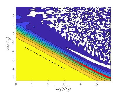
Scaling behaviour is particularly apparent when represented in the $(\log(t),\log(k))$ plane. Indeed, it this logarithmic representation, scaling simply corresponds to equal values of the correlation $\Gamma(k,t)$ along straight lines.

Figure 1 shows contour plots of the normalized correlation function $\tilde{\Gamma}(k,t)=\Gamma(k,t)/\Gamma(k,0)$. The red circles indicate the points $t=\tau_{\frac{1}{2}}(k)$. They were computed independently, for each $k$, by solving the equation $\Gamma(k,\tau_{\frac{1}{2}})={\frac{1}{2}}\Gamma(k,0)$.

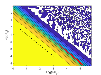
The left panel of Figure 1 shows the inviscid Burgers scaling that is obtained for $\nu=0$, corresponding to an infinite truncation-scale Reynolds number $R_{\rm min}$. The black solid line indicates the theoretical $t\sim k^{-1}$ law. On the right panel, the KPZ scaling obtained at $\nu=3.0\times 10^{-3}$ is displayed, corresponding to a truncation-scale Reynolds number $R_{\rm min}=0.98$. The black solid lines indicating the theoretical $t\sim k^{-3/2}$ law.

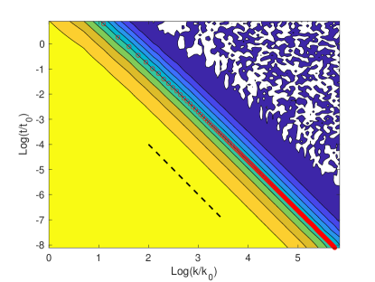
The left panel of Figure 2 demonstrates the EW scaling that is obtained with $\nu=2.4\times 10^{-2}$, corresponding to a truncation-scale Reynolds number of $R_{\rm min}=0.12$. The viscous $t\sim k^{-2}$ EZ law is indicated by the black solid line. The right panel shows the crossover in the scaling of the decorrelation times $\tau_{\frac{1}{2}}(k)$ versus $k$ for various values of the viscosity $\nu$.

Figure 3: Crossover in the scaling of the decorrelation time $\tau_{\frac{1}{2}}$ for the same conditions as in Figure 2 (right panel), but compensated by $k^{3/2}$: $k^{3/2}\tau_{\frac{1}{2}}$ versus $k$. Red circles correspond to the EW to KPZ transition: $\nu=2.4\times 10^{-2}$, $\nu=1.2\times 10^{-2}$, $\nu=6.0\times 10^{-3}$ and $\nu=3.0\times 10^{-3}$ and green diamond correspond to the KPZ to inviscid transition: $\nu=1.5\times 10^{-3}$, $\nu=7.5\times 10^{-4}$, $\nu=3.8\times 10^{-4}$, $\nu=1.9\times 10^{-5}$, $\nu=9.4\times 10^{-6}$, $\nu=4.7\times 10^{-6}$, and $\nu=0$. Scaling laws are indicated by solid lines: EW $k^{-2}$ and KPZ $k^{-3/2}$. The new inviscid $k^{-1}$ scaling is denoted by a dashed line. Runs performed with $k_{\rm max}=341$ and $u_{rms}=1$.

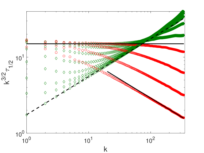
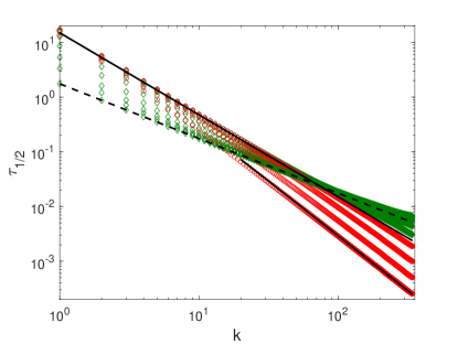
The crossover behaviour is clearly visible in Figure 3 that displays the same data compensated by $k^{3/2}$, so that KPZ scaling corresponds to a horizontal line. The red circles correspond to the EW to KPZ transition with various values of viscosities in geometric progression corresponding to a truncation-scale Reynolds number: $R_{\rm min}=0.12$, $R_{\rm min}=0.24$, $R_{\rm min}=0.98$. The green diamond correspond to the KPZ to inviscid transition, with various viscosities, also in geometric progression corresponding to a truncation-scale Reynolds number: $R_{\rm min}=1.96$, $R_{\rm min}=3.91$, $R_{\rm min}=7.71$, $R_{\rm min}=15.4$, $R_{\rm min}=31.2$, $R_{\rm min}=62.3$ and $R_{\rm min}=\infty$ . The EW $k^{-2}$ scaling law and the KPZ $k^{-3/2}$ scaling are indicated by solid lines and the inviscid $k^{-1}$ scaling is denoted by a dashed line.

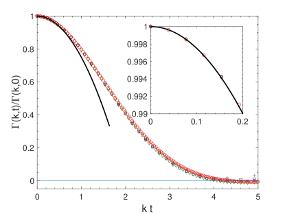
Figure 4 shows the scaling form of the normalized correlation functions $\Gamma(k,t)/\Gamma(k,0)$ versus the rescaled wavenumber, with the same conditions as in Fig.1, Fig.2 and Fig.3.

Figure 4: Scaling of correlation functions $\Gamma(k,t)/\Gamma(k,0)$ versus the rescaled wavenumber. Left: KPZ ($\nu=.003$) correlation versus $k(t/7.0)^{2/3}$ (o: $k=4$, diamond: $k=8$, square: $k=16$, v: $k=32$ and +: $k=64$) compared with the theoretical correlation function computed in reference [35] shown by a solid line (the inset shows the change of sign of the theoretical correlation); right Inviscid ($\nu=0$) correlation versus $kt$ (o: $k=8$, diamond: $k=16$, square: $k=32$, v: $k=64$ and +: $k=128$) compared with the theoretical short-time parabolic behaviour (see inset and Eq. (29)). Computations were performed with $k_{\rm max}=341$ and $u_{rms}=1$

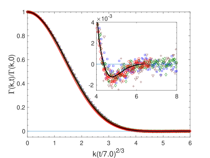
The left panel shows the KPZ correlation (obtained at $\nu=.003$), plotted versus the rescaled variable $k(t/7.0)^{2/3}$ for various values of $k$. The theoretical correlation function, computed in reference [35], is shown as a solid black line. The inset provides details on the change of sign of the correlation.

The right panel displays the inviscid ($\nu=0$) correlation versus the rescaled variable $kt$, for various values of $k$. The theoretical short-time parabolic behaviour is shown as a black continuous curve. The inset shows short-times details. The inviscid parabolic law can be obtained by the following arguments. Starting from the equilibrium correlation functions $\left<\hat{u}({k},t)\hat{u}({k^{\prime}},0)\right>$, we can define the time scale $\tau_{\rm C}$ as the parabolic decorrelation time

$$\tau_{\rm C}^{2}\partial_{tt}\left<\hat{u}({k},t)\hat{u}({k^{\prime}},0)\right>_{|t=0}=\left<\hat{u}({k},0)\hat{u}({k^{\prime}},0)\right>,$$ (27)

time translation invariance allows us to express the second order time derivative as

$$-\left<{\partial_{t}\hat{v}}({k},t)\partial_{t^{\prime}}\hat{u}({k^{\prime}},t^{\prime})\right>_{|t=t^{\prime}=0}.$$ (28)

Using expressions (11) for the time derivatives reduces the evaluation of $\tau_{\rm C}$ to that of an equal-time fourth-order moment of a Gaussian field with correlation $<\hat{u}({k},t)\hat{u}({-k},t)>=u_{\rm rms}^{2}/(2k_{\rm max}+1)$. The only non-vanishing contribution is a one loop graph [36, 27]. The correlation time $\tau_{\rm C}$ associated to wavenumber $k$ is found [19, 6] in this way to obey the simple scaling law

$$\tau_{\rm C}=\frac{\sqrt{2}}{ku_{\rm rms}},$$ (29)

and this time-scale is proportional to the eddy turnover time [17] at wavenumber $k$.

It is apparent from the Figure that our numerical data obey the theoretical predictions.

3.4 Distributions of the interface increments

Figure 5: Left: probability distribution functions of the interface increments $\delta h$ at times $t=0.5$, $t=1$, $t=2$, $t=4$ and $t=8$, with $\nu=3.0\times 10^{-3}$, $k_{\rm max}=682$ and $u_{rms}=1$; (right) time evolution of the skewness (green) and excess kurtosis (red) at various viscosities in log-log scales. The solid black lines indicate the theoretical results of reference [26]. The markers correspond to: inviscid $(\nu=0$): +, $\nu=3.8\times 10^{-4}$: o, $\nu=7.5\times 10^{-4}$: asterisk, $\nu=1.5\times 10^{-3}$: square, $\nu=3.0\times 10^{-3}$: diamond, $\nu=6.0\times 10^{-3}$: pentagram, $\nu=1.2\times 10^{-2}$: hexagram;

The seminal work of Prähofer and Spohn [37] was recently referred to as “the $2^{nd}$ KPZ Revolution” [23]. It has led to a new set of studies of the 1D KPZ universality class [38, 39, 40, 41, 26, 24, 42]. In particular, Ref. [43] notes that, at $x$ and large $t$

$$\delta h=h(x,t)-h(x,0)\approx v_{\infty}t+(\Gamma t)^{\beta_{\text{KPZ}}}\chi_{\beta}+o(t^{\beta_{\text{KPZ}}})\ ,\ \text{for}\ t\rightarrow\infty,$$ (30)

where the parameters $\Gamma$ and $v_{\infty}$ depend on the model, and $\beta_{\text{KPZ}}=1/3$. Furthermore, $\chi_{\beta}$ is a random variable distributed according to different (Tracy-Widom) distributions [44] for different initial conditions. For the problem we study, we use Brownian initial data, so we expect (see Ref. [43]) to find a Baik-Rains [45] distribution.

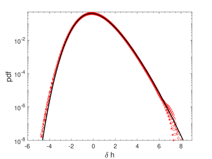
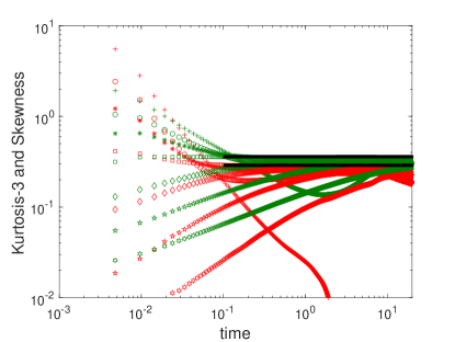
Figure 5 shows the evolution of the distributions of the interface increments $\delta h$ computed with $k_{\rm max}=682$ and $u_{rms}=1$. The left panel displays the probability distribution functions of $\delta h$ at various times and $\nu=3.0\times 10^{-3}$. The solid black curve indicates the theoretical probability distribution function of reference [26]. The right panels show the time evolution of the skewness $S$ (in green) and excess kurtosis $K-3$ (in red) at various viscosities.

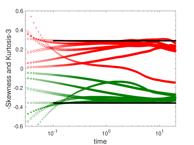
Figure 6 displays the same data, with a change of sign for the skewness (in order to be comparable with Figure 3 of Ref. [43]). Our results indicate a tendency for the viscous run to converge towards the theoretically predicted values, while the inviscid computation only display power law behaviour for the skewness and the excess flatness.

4 Conclusion

Figure 6: Time evolution of the skewness (green) and excess kurtosis (red) at various viscosities in log-lin scales (same conditions as in Figure 5 right, with a change of sign for the skewness). The solid black lines indicate the theoretical results of reference [26]. The markers correspond to: inviscid $(\nu=0$): +, $\nu=3.8\times 10^{-4}$: o, $\nu=7.5\times 10^{-4}$: asterisk, $\nu=1.5\times 10^{-3}$: square, $\nu=3.0\times 10^{-3}$: diamond, $\nu=6.0\times 10^{-3}$: pentagram, $\nu=1.2\times 10^{-2}$: hexagram;

By using pseudospectral numerical simulations of the $1D$ Galerkin-truncated Burgers equation, with noise and dissipation (2), we have reproduced the very well known properties of the $1D$ KPZ universality class such as the $k^{-3/2}$ scaling of the correlation time, the known analytical forms for the rescaled time-correlation function and the rescaled interface increments probability distribution function.

We have characterised a new crossover, controlled by the truncation-scale Reynolds number $R_{\rm min}$, towards an inviscid regime with correlation time scaling as $k^{-1}$. This new regime correspond to the absolute equilibrium solutions of the inviscid noiseless Burgers equation. To obtain this regime, it is crucial that the numerical scheme exactly conserves the invariant energy of the system. This inviscid regime should also be present in finite-difference schemes, provided that they also conserve the invariants (see the discussions in Refs. [17, 18]). On general grounds, one expects that any model within the $1D$ KPZ universality class could also exhibit this new crossover provided that it also admits exact conservations laws in some well-defined non-dissipative limit.

This new regime might be amenable to a renormalization-group analysis, which would have, in addition to the known [21] KPZ stable fixed point and EW unstable fixed point, a new fixed point corresponding to the inviscid regime. This is left for a future work.

All authors participated in the analytical computations. MB and RP drafted the manuscript. MB and CC performed the numerical simulations. CC RP and MB read, edited and approved the manuscript. Enrique Tirapegui was instrumental in the early definition of the research project and the corresponding analytical computations. He sadly passed away in 2020 and could not therefore edit and approve to the final manuscript. The authors declare that they have no competing interests. This work was supported by the French Agence nationale de la recherche (ANR QUTE-HPC project No. ANR-18-CE46-0013). This work was granted access to HPC resources of MesoPSL financed by Region Ile de France and the project Equip@Meso (reference ANR-10-EQPX-29-01) of the programme Investissements d’Avenir supervised by Agence Nationale pour la Recherche. MB and RP thank the Indo-French Centre for Applied Mathematics for financial support. RP also thanks CSIR, UGC, and DST India for support and Dipankar Roy for discussions. CC, ET and MB acknowledge the support of the Laboratoire International Associé "Matier̀e: Structure et Dynamique" LIA-MSD. CC wishes to acknowledge the support of FONDECYT (CL), No. 1200357 and Universidad de los Andes (CL) through FAI initiatives.

References

- [1] T. D. Lee, “On some statistical properties of hydrodynamical and magneto-hydrodynamical fields,” Quart Appl Math, vol. 10, no. 1, pp. 69–74, 1952.
- [2] E. Hopf, “Statistical hydromechanics and functional calculus,” Journal of rational Mechanics and Analysis, vol. 1, pp. 87–123, 1952.
- [3] R. Kraichnan, “On the statistical mechanics of an adiabatically compressible fluid,” J. Acoust. Soc. Am., vol. 27, no. 3, pp. 438–441, 1955.
- [4] R. Kraichnan, “Helical turbulence and absolute equilibrium,” J. Fluid Mech., vol. 59, pp. 745–752, 1973.
- [5] S. Orszag, Statistical Theory of Turbulence. in, Les Houches 1973: Fluid dynamics, R. Balian and J.L. Peube eds. Gordon and Breach, New York, 1977.
- [6] C. Cichowlas, P. Bonaïti, F. Debbasch, and M. Brachet, “Effective dissipation and turbulence in spectrally truncated Euler flows,” Physical Review Letters, vol. 95, no. 26, p. 264502, 2005.
- [7] G. Krstulovic, P. D. Mininni, M. E. Brachet, and A. Pouquet, “Cascades, thermalization, and eddy viscosity in helical Galerkin truncated Euler flows,” Phys. Rev. E, pp. 1–5, May 2009.
- [8] D. Gottlieb and S. A. Orszag, Numerical Analysis of Spectral Methods. Philadelphia: SIAM, 1977.
- [9] C. Canuto, M. Y. Hussani, A. Quarteroni, and T. A. Zang, Spectral Methods in Fluid Dynamics. New York and Berlin: Springer-Verlag, 2nd printing ed., 1988.
- [10] G. Krstulovic, C. Cartes, M. Brachet, and E. Tirapegui, “Generation and charecterization of absolute equilibrium of compressible flows,” International Journal of Bifurcation and Chaos, vol. 19, no. 10, pp. 3445–3459, 2009.
- [11] G. Krstulovic and M. E. Brachet, “Dispersive bottleneck delaying thermalization of turbulent Bose-Einstein condensates,” Phys. Rev. Lett, vol. 106, p. 115303, 2011.
- [12] V. Shukla, M. Brachet, and R. Pandit, “Turbulence in the two-dimensional Fourier-truncated Gross-Pitaevskii equation,” New J. Phys., vol. 15, no. 11, p. 113025, 2013.
- [13] G. Krstulovic, M.-E. Brachet, and A. Pouquet, “Alfvén waves and ideal two-dimensional Galerkin truncated magnetohydrodynamics,” Phys. Rev. E, vol. 84, p. 016410, Jul 2011.
- [14] S. S. Ray, U. Frisch, S. Nazarenko, and T. Matsumoto, “Resonance phenomenon for the Galerkin-truncated Burgers and Euler equations,” Phys. Rev. E, vol. 84, p. 016301, 2011.
- [15] D. Banerjee and S. S. Ray, “Transition from dissipative to conservative dynamics in equations of hydrodynamics,” Phys. Rev. E, vol. 90, p. 041001, Oct 2014.
- [16] S. S. Ray, “Thermalized solutions, statistical mechanics and turbulence: An overview of some recent results,” Pramana, vol. 84, no. 3, pp. 395–407, 2015.
- [17] A. J. Majda and I. Timofeyev, “Remarkable statistical behavior for truncated Burgers-Hopf dynamics,” Proceedings of the National Academy of Sciences, vol. 97, no. 23, pp. 12413–12417, 2000.
- [18] A. Majda and I. Timofeyev, “Statistical mechanics for truncations of the Burgers-Hopf equation: A model for intrinsic stochastic behavior with scaling,” Milan Journal of Mathematics, vol. 70, no. 1, pp. 39–96, 2002.
- [19] C. Cichowlas, Truncated Euler Equation: from complex singularities dynamics to turbulent relaxation. PhD thesis, Universite Pierre et Marie Curie - Paris VI, https://tel.archives-ouvertes.fr/tel-00070819/document, 2005.
- [20] D. Forster, D. R. Nelson, and M. J. Stephen, “Large-distance and long-time properties of a randomly stirred fluid,” Phys. Rev. A, vol. 16, pp. 732–749, Aug 1977.
- [21] M. Kardar, G. Parisi, and Y.-C. Zhang, “Dynamic scaling of growing interfaces,” Phys. Rev. Lett., vol. 56, pp. 889–892, Mar 1986.
- [22] T. Halpin-Healy and Y.-C. Zhang, “Kinetic roughening phenomena, stochastic growth, directed polymers and all that. aspects of multidisciplinary statistical mechanics,” Physics Reports, vol. 254, no. 4, pp. 215 – 414, 1995.
- [23] T. Halpin-Healy and K. A. Takeuchi, “A KPZ cocktail-shaken, not stirred…,” Journal of Statistical Physics, vol. 160, pp. 794–814, Aug 2015.
- [24] J. Quastel and H. Spohn, “The one-dimensional KPZ equation and its universality class,” Journal of Statistical Physics, vol. 160, pp. 965–984, Aug 2015.
- [25] S. F. Edwards and D. R. Wilkinson, “The surface statistics of a granular aggregate,” Proceedings of the Royal Society of London. A. Mathematical and Physical Sciences, vol. 381, no. 1780, pp. 17–31, 1982.
- [26] T. Halpin-Healy and Y. Lin, “Universal aspects of curved, flat, and stationary-state Kardar-Parisi-Zhang statistics,” Phys. Rev. E, vol. 89, p. 010103, Jan 2014.
- [27] U. Frisch, Turbulence: The Legacy of A. N. Kolmogorov. Cambridge University Press, 1995.
- [28] U. Frisch and J. Bec, “Burgulence,” in New trends in turbulence Turbulence: nouveaux aspects: 31 July – 1 September 2000 (M. Lesieur, A. Yaglom, and F. David, eds.), (Berlin, Heidelberg), pp. 341–383, Springer Berlin Heidelberg, 2001.
- [29] J. Bec and K. Khanin, “Burgers turbulence,” Physics Reports, vol. 447, no. 1, pp. 1–66, 2007.
- [30] R. V. Abramov, G. Kovačič, and A. J. Majda, “Hamiltonian structure and statistically relevant conserved quantities for the truncated Burgers-Hopf equation,” Communications on Pure and Applied Mathematics, vol. 56, no. 1, pp. 1–46, 2003.
- [31] N. G. v. Kampen, Stochastic processes in physics and chemistry. North-Holland ; sole distributors for the USA and Canada, Elsevier North-Holland, Amsterdam ; New York : New York :, 1981.
- [32] F. Langouche, D. Roekaerts, and E. Tirapegui, Functional integration and semiclassical expansions. D Reidel Pub Co, Jan 1982.
- [33] R. Kraichnan, “Classical fluctuation-relaxation theorem,” Phys. Rev., vol. 113, no. 5, pp. 1181,1182, 1959.
- [34] V. Mannella, R.and Palleschi, “Fast and precise algorithm for computer simulation of stochastic differential equations,” Phys.Rev.A, vol. 40, pp. 3381– 3386, Sep 1989.
- [35] M. Prähofer and H. Spohn, “Exact scaling functions for one-dimensional stationary KPZ growth,” Journal of Statistical Physics, vol. 115, pp. 255–279, Apr 2004.
- [36] L. Isserlis, “On a formula for the product-moment coefficient in any number of variables,” Biometrika, vol. 12, pp. 134,139, 1918.
- [37] M. Prähofer and H. Spohn, “Universal distributions for growth processes in dimensions and random matrices,” Phys. Rev. Lett., vol. 84, pp. 4882–4885, May 2000.
- [38] T. Sasamoto and H. Spohn, “One-dimensional Kardar-Parisi-Zhang equation: An exact solution and its universality,” Phys. Rev. Lett., vol. 104, p. 230602, Jun 2010.
- [39] P. Calabrese and P. Le Doussal, “Exact solution for the Kardar-Parisi-Zhang equation with flat initial conditions,” Phys. Rev. Lett., vol. 106, p. 250603, Jun 2011.
- [40] T. Imamura and T. Sasamoto, “Exact solution for the stationary Kardar-Parisi-Zhang equation,” Phys. Rev. Lett., vol. 108, p. 190603, May 2012.
- [41] I. Corwin, “The Kardar-Parisi-Zhang equation and universality class,” Random Matrices: Theory and Applications, vol. 01, no. 01, p. 1130001, 2012.
- [42] A. A. Saberi, H. Dashti-Naserabadi, and J. Krug, “Competing universalities in Kardar-Parisi-Zhang growth models,” Phys. Rev. Lett., vol. 122, p. 040605, Jan 2019.
- [43] D. Roy and R. Pandit, “One-dimensional Kardar-Parisi-Zhang and Kuramoto-Sivashinsky universality class: Limit distributions,” Phys. Rev. E, vol. 101, p. 030103, Mar 2020.
- [44] C. A. Tracy and H. Widom, “Level-spacing distributions and the Airy kernel,” Communications in Mathematical Physics, vol. 159, pp. 151–174, Jan 1994.
- [45] J. Baik and E. M. Rains, “Limiting distributions for a polynuclear growth model with external sources,” Journal of Statistical Physics, vol. 100, pp. 523–541, Aug 2000.