Consistency of Constrained Spectral Clustering under Graph Induced Fair Planted Partitions

Abstract

Spectral clustering is popular among practitioners and theoreticians alike. While performance guarantees for spectral clustering are well understood, recent studies have focused on enforcing “fairness” in clusters, requiring them to be “balanced” with respect to a categorical sensitive node attribute (e.g. the race distribution in clusters must match the race distribution in the population). In this paper, we consider a setting where sensitive attributes indirectly manifest in an auxiliary representation graph rather than being directly observed. This graph specifies node pairs that can represent each other with respect to sensitive attributes and is observed in addition to the usual similarity graph. Our goal is to find clusters in the similarity graph while respecting a new individual-level fairness constraint encoded by the representation graph. We develop variants of unnormalized and normalized spectral clustering for this task and analyze their performance under a fair planted partition model induced by the representation graph. This model uses both the cluster membership of the nodes and the structure of the representation graph to generate random similarity graphs. To the best of our knowledge, these are the first consistency results for constrained spectral clustering under an individual-level fairness constraint. Numerical results corroborate our theoretical findings.

1 Introduction

Consider a recommendation service that groups news articles by finding clusters in a graph which connects these articles via cross-references. Unfortunately, as cross-references between articles with different political viewpoints are uncommon, this service risks forming ideological filter bubbles. To counter polarization, it must ensure that clusters on topics like finance and healthcare include a diverse range of opinions. This is an example of a constrained clustering problem. The popular spectral clustering algorithm (Ng et al., 2001; von Luxburg, 2007) has been adapted over the years to include constraints such as must-link and cannot-link constraints (Kamvar et al., 2003; Wang and Davidson, 2010), size-balanced clusters (Banerjee and Ghosh, 2006), and statistical fairness (Kleindessner et al., 2019). These constraints can be broadly divided into two categories: (i) Population level constraints that must be satisfied by the clusters as a whole (e.g. size-balanced clusters and statistical fairness); and (ii) Individual level constraints that must be satisfied at the level of individual nodes (e.g. must/cannot link constraints). To the best of our knowledge, the only known statistical consistency guarantees for constrained spectral clustering were studied in Kleindessner et al. (2019) in the context of a population level fairness constraint where the goal is to find clusters that are balanced with respect to a categorical sensitive node attribute. In this paper, we establish consistency guarantees for constrained spectral clustering under a new and more general individual level fairness constraint.

Informal problem description:

We assume the availability of two graphs: a similarity graph $\mathcal{G}$ in which the clusters are to be found and a representation graph $\mathcal{R}$, defined on the same set of nodes as $\mathcal{G}$, which encodes the “is representative of” relationship. Our goal is to find clusters in $\mathcal{G}$ such that every node has a sufficient number of its representatives from $\mathcal{R}$ in all clusters. For example, $\mathcal{G}$ may be a graph of consumers based on the similarity of their purchasing habits and $\mathcal{R}$ may be a graph based on the similarity of their sensitive attributes such as gender, race, and sexual orientation. This, for instance, would then be a step towards reducing discrimination in online marketplaces (Fisman and Luca, 2016).

Contributions and results:

First, in Section 3.1, we formalize our new individual level fairness constraint for clustering, called the representation constraint. It is different from most existing fairness notions which either apply at the population level (Chierichetti et al., 2017; Rösner and Schmidt, 2018; Bercea et al., 2019; Bera et al., 2019) or are hard to integrate with spectral clustering (Chen et al., 2019; Mahabadi and Vakilian, 2020; Anderson et al., 2020). Unlike these notions, our constraint can be used with multiple sensitive attributes of different types (categorical, numerical etc.) and only requires observing an abstract representation graph based on these attributes rather than requiring their actual values, thereby discouraging individual profiling. Appendix A discusses the utility of individual fairness notions.

Second, in Section 3.2, we develop the representation-aware variant of unnormalized spectral clustering to find clusters that approximately satisfy the proposed constraint. An analogous variant for normalized spectral clustering is presented in Section B.2.

Third, in Section 4.1, we introduce $\mathcal{R}$-PP, a new representation-aware (or fair) planted partition model. This model generates random similarity graphs $\mathcal{G}$ conditioned on both the cluster membership of nodes and a given representation graph $\mathcal{R}$. Intuitively, $\mathcal{R}$-PP plants the properties of $\mathcal{R}$ in $\mathcal{G}$. We show that this model generates “hard” problem instances and establish the weak consistency of our algorithms under this model for a class of $d$-regular representation graphs (Theorems 4.1 and 4.2). To the best of our knowledge, these are the first consistency results for constrained spectral clustering under an individual-level constraint. In fact, we show that our results imply the only other similar consistency result (but for a population-level constraint) in Kleindessner et al. (2019) as a special case (Appendix A).

Finally, fourth, we present empirical results on both real and simulated data to corroborate our theoretical findings (Section 5). In particular, our experiments show that our algorithms perform well in practice, even when the $d$-regularity assumption on $\mathcal{R}$ is violated.

Related work:

Spectral clustering has been modified to satisfy individual level must-link and cannot-link constraints by pre-processing the similarity graph (Kamvar et al., 2003), post-processing the eigenvectors of the graph Laplacian (Li et al., 2009), and modifying its optimization problem (Yu and Shi, 2001; Yu and Shi, 2004; Wang and Davidson, 2010; Wang et al., 2014; Cucuringu et al., 2016). It has also been extended to accommodate various population level constraints (Banerjee and Ghosh, 2006; Xu et al., 2009). We are unaware of theoretical performance guarantees for any of these algorithms.

Of particular interest to us are the fairness constraints for clustering. One popular population level constraint requires sensitive attributes to be proportionally represented in clusters (Chierichetti et al., 2017; Rösner and Schmidt, 2018; Bercea et al., 2019; Bera et al., 2019; Esmaeili et al., 2020, 2021). For example, if $50\%$ of the population is female then the same proportion should be respected in all clusters. Several efficient algorithms for discovering such clusters have been proposed (Schmidt et al., 2018; Ahmadian et al., 2019; Harb and Shan, 2020), though they almost exclusively focus on variants of $k$-means while we are interested in spectral clustering. Kleindessner et al. (2019) deserve a special mention as they develop a spectral clustering algorithm for this fairness notion. However, we recover all the results presented in Kleindessner et al. (2019) as a special case of our analysis as our proposed constraint interpolates between population level and individual level fairness based on the structure of $\mathcal{R}$. While individual fairness notions for clustering have also been explored (Chen et al., 2019; Mahabadi and Vakilian, 2020; Anderson et al., 2020; Chakrabarty and Negahbani, 2021), none of them have previously been used with spectral clustering. See Caton and Haas (2020) for a broader discussion on fairness.

A final line of relevant work concerns consistency results for variants of unconstrained spectral clustering. von Luxburg et al. (2008) established the weak consistency of spectral clustering assuming that the similarity graph $\mathcal{G}$ encodes cosine similarity between examples using feature vectors drawn from a particular probability distribution. Rohe et al. (2011) and Lei and Rinaldo (2015) assume that $\mathcal{G}$ is sampled from variants of the Stochastic Block Model (SBM) (Holland et al., 1983). Zhang et al. (2014) allow clusters to overlap. Binkiewicz et al. (2017) consider auxiliary node attributes, though, unlike us, their aim is to find clusters that are well aligned with these attributes. A faster variant of spectral clustering was analyzed by Tremblay et al. (2016). Spectral clustering has also been studied on other types of graphs such as hypergraphs (Ghoshdastidar and Dukkipati, 2017a, b) and strong consistency guarantees are also known (Gao et al., 2017; Lei and Zhu, 2017; Vu, 2018), albeit under stronger assumptions.

Notation:

Define $[n]\coloneqq\{1,2,\dots,n\}$ for any integer $n$. Let $\mathcal{G}=(\mathcal{V},\mathcal{E})$ denote a similarity graph, where $\mathcal{V}=\{v_{1},v_{2},\dots,v_{N}\}$ is the set of $N$ nodes and $\mathcal{E}\subseteq\mathcal{V}\times\mathcal{V}$ is the set of edges. Clustering aims to partition the nodes in $\mathcal{G}$ into $K\geq 2$ non-overlapping clusters $\mathcal{C}_{1},\dots,\mathcal{C}_{K}\subseteq\mathcal{V}$. We assume the availability of another graph, called a representation graph $\mathcal{R}=(\mathcal{V},\hat{\mathcal{E}})$, which is defined on the same set of vertices as $\mathcal{G}$ but with different edges $\hat{\mathcal{E}}$. The discovered clusters $\mathcal{C}_{1},\dots,\mathcal{C}_{K}$ are required to satisfy a fairness constraint encoded by $\mathcal{R}$, as described in Section 3.1. $\mathbf{A},\mathbf{R}\in\{0,1\}^{N\times N}$ denote the adjacency matrices of graphs $\mathcal{G}$ and $\mathcal{R}$, respectively. We assume that $\mathcal{G}$ and $\mathcal{R}$ are undirected and that $\mathcal{G}$ has no self-loops.

2 Unnormalized spectral clustering

We begin with a brief review of unnormalized spectral clustering which will be useful in describing our algorithm in Section 3.2. The normalized variants of traditional spectral clustering and our algorithm have been deferred to Appendix B. Given a similarity graph $\mathcal{G}$, unnormalized spectral clustering finds clusters by approximately minimizing the following metric known as ratio-cut (von Luxburg, 2007)

$$\mathrm{RCut}(\mathcal{C}_{1},\dots,\mathcal{C}_{K})=\sum_{i=1}^{K}\frac{\mathrm{Cut}(\mathcal{C}_{i},\mathcal{V}\backslash\mathcal{C}_{i})}{|\mathcal{C}_{i}|}.$$

Here, $\mathcal{V}\backslash\mathcal{C}_{i}$ is the set difference between $\mathcal{V}$ and $\mathcal{C}_{i}$. For any two subsets $\mathcal{X},\mathcal{Y}\subseteq\mathcal{V}$, $\mathrm{Cut}(\mathcal{X},\mathcal{Y})=\frac{1}{2}\sum_{v_{i}\in\mathcal{X},v_{j}\in\mathcal{Y}}A_{ij}$ counts the number of edges that have one endpoint in $\mathcal{X}$ and another in $\mathcal{Y}$. Let $\mathbf{D}\in\mathbb{R}^{N\times N}$ be a diagonal degree matrix where $D_{ii}=\sum_{j=1}^{N}A_{ij}$ for all $i\in[N]$. It is easy to verify that ratio-cut can be expressed in terms of the graph Laplacian $\mathbf{L}\coloneqq\mathbf{D}-\mathbf{A}$ and a cluster membership matrix $\mathbf{H}\in\mathbb{R}^{N\times K}$ as $\mathrm{RCut}(\mathcal{C}_{1},\dots,\mathcal{C}_{K})=\mathrm{trace}\{\mathbf{H}^{\intercal}\mathbf{L}\mathbf{H}\}$, where

$$H_{ij}=\begin{cases}\frac{1}{\sqrt{|\mathcal{C}_{j}|}}&\text{ if }v_{i}\in\mathcal{C}_{j}\\ 0&\text{ otherwise.}\end{cases}$$ (1)

Thus, to find good clusters, one can minimize $\mathrm{trace}\{\mathbf{H}^{\intercal}\mathbf{L}\mathbf{H}\}$ over all $\mathbf{H}$ that have the form given in (1). However, the combinatorial nature of this constraint makes this problem NP-hard (Wagner and Wagner, 1993). Unnormalized spectral clustering instead solves the following relaxed problem:

$$\min_{\mathbf{H}\in\mathbb{R}^{N\times K}}\,\,\,\,\mathrm{trace}\{\mathbf{H}^{\intercal}\mathbf{L}\mathbf{H}\}\,\,\,\,\text{s.t.}\,\,\,\,\mathbf{H}^{\intercal}\mathbf{H}=\mathbf{I}.$$ (2)

Note that $\mathbf{H}$ in (1) satisfies $\mathbf{H}^{\intercal}\mathbf{H}=\mathbf{I}$. The above relaxation is often referred to as the spectral relaxation. By Rayleigh-Ritz theorem (Lütkepohl, 1996, Section 5.2.2), the optimal matrix $\mathbf{H}^{*}$ is such that it has $\mathbf{u}_{1},\mathbf{u}_{2},\dots,\mathbf{u}_{K}\in\mathbb{R}^{N}$ as its columns, where $\mathbf{u}_{i}$ is the eigenvector corresponding to the $i^{th}$ smallest eigenvalue of $\mathbf{L}$ for all $i\in[K]$. The algorithm clusters the rows of $\mathbf{H}^{*}$ into $K$ clusters using $k$-means clustering (Lloyd, 1982) to return $\hat{\mathcal{C}}_{1},\dots,\hat{\mathcal{C}}_{K}$. Algorithm 1 summarizes this procedure. Unless stated otherwise, we will use spectral clustering (without any qualification) to refer to unnormalized spectral clustering.

1:Input: Adjacency matrix $\mathbf{A}$, number of clusters $K\geq 2$

2:Compute the Laplacian matrix $\mathbf{L}=\mathbf{D}-\mathbf{A}$.

3:Compute the first $K$ eigenvectors $\mathbf{u}_{1},\dots,\mathbf{u}_{K}$ of $\mathbf{L}$. Let $\mathbf{H}^{*}\in\mathbb{R}^{N\times K}$ be a matrix that has $\mathbf{u}_{1},\dots,\mathbf{u}_{K}$ as its columns.

4:Let $\mathbf{h}^{*}_{i}$ denote the $i^{th}$ row of $\mathbf{H}^{*}$. Cluster $\mathbf{h}^{*}_{1},\dots,\mathbf{h}^{*}_{N}$ into $K$ clusters using $k$-means clustering.

5:Output: Clusters $\hat{\mathcal{C}}_{1},\dots,\hat{\mathcal{C}}_{K}$, s.t. $\hat{\mathcal{C}}_{i}=\{v_{j}\in\mathcal{V}:\mathbf{h}^{*}_{j}\text{ was assigned to the }i^{th}\text{ cluster}\}$.

Algorithm 1 Unnormalized spectral clustering

3 Representation constraint and representation-aware spectral clustering

In this section, we first describe our individual level fairness constraint in Section 3.1 and then develop Unnormalized Representation-Aware Spectral Clustering in Section 3.2 to find clusters that approximately satisfy this constraint. See Appendix B for the normalized variant of the algorithm.

3.1 Representation constraint

A representation graph $\mathcal{R}$ connects nodes that represent each other based on sensitive attributes (e.g. political opinions). Let $\mathcal{N}_{\mathcal{R}}(i)=\{v_{j}\;:\;R_{ij}=1\}$ be the set of neighbors of node $v_{i}$ in $\mathcal{R}$. The size of $\mathcal{N}_{\mathcal{R}}(i)\cap\mathcal{C}_{k}$ specifies node $v_{i}$’s representation in cluster $\mathcal{C}_{k}$. To motivate our constraint, consider the following notion of balance $\rho_{i}$ of clusters defined from the perspective of a particular node $v_{i}$:

$$\rho_{i}=\min_{k,\ell\in[K]}\;\;\frac{|\mathcal{C}_{k}\cap\mathcal{N}_{\mathcal{R}}(i)|}{|\mathcal{C}_{\ell}\cap\mathcal{N}_{\mathcal{R}}(i)|}$$ (3)

It is easy to see that $0\leq\rho_{i}\leq 1$ and higher values of $\rho_{i}$ indicate that node $v_{i}$ has an adequate representation in all clusters. Thus, one objective could be to find clusters $\mathcal{C}_{1},\dots,\mathcal{C}_{K}$ that solve the following optimization problem.

$$\min_{\mathcal{C}_{1},\dots,\mathcal{C}_{K}}\;\;f(\mathcal{C}_{1},\dots,\mathcal{C}_{K})\;\;\;\;\text{s.t.}\;\;\;\;\rho_{i}\geq\alpha,\;\forall\;i\in[N],$$ (4)

where $f(\cdot)$ is inversely proportional to the quality of clusters (such as $\mathrm{RCut}$) and $\alpha\in[0,1]$ is a user specified threshold. However, it is not clear how this approach can be combined with spectral clustering to develop a consistent algorithm. We take a different approach described below.

First, note that $\min_{i\in[N]}\rho_{i}\leq\min_{k,\ell\in[K]}\;\frac{|\mathcal{C}_{k}|}{|\mathcal{C}_{\ell}|}$. Therefore, the balance $\rho_{i}$ of the least balanced node $v_{i}$ is maximized when its representatives $\mathcal{N}_{\mathcal{R}}(i)$ are split across clusters $\mathcal{C}_{1},\dots,\mathcal{C}_{K}$ in proportion to their sizes. Representation constraint requires this condition to be satisfied for each node in the graph.

Definition 3.1 (Representation constraint).

Given a representation graph $\mathcal{R}$, clusters $\mathcal{C}_{1},\dots,\mathcal{C}_{K}$ in $\mathcal{G}$ satisfy the representation constraint if $|\mathcal{C}_{k}\cap\mathcal{N}_{\mathcal{R}}(i)|\propto|\mathcal{C}_{k}|$ for all $i\in[N]$ and $k\in[K]$, i.e.,

$$\frac{|\mathcal{C}_{k}\cap\mathcal{N}_{\mathcal{R}}(i)|}{|\mathcal{C}_{k}|}=\frac{|\mathcal{N}_{\mathcal{R}}(i)|}{N},\;\;\forall k\in[K],\;\forall i\in[N].$$ (5)

In other words, the representation constraint requires the representatives of any given node to have a proportional membership in all clusters. For example, if $v_{i}$ is connected to $30\%$ of all nodes in $\mathcal{R}$, then it must have $30\%$ representation in all clusters discovered in $\mathcal{G}$. It is important to note that this constraint applies at the level of individual nodes unlike population level constraints (Chierichetti et al., 2017).

While (4) can always be solved for a small enough value of $\alpha$ (with the convention that $0/0=1$), the constraint in Definition 3.1 may not always be feasible. For example, (5) can never be satisfied if a node has only two representatives (i.e., $|\mathcal{N}_{\mathcal{R}}(i)|=2$) and there are $K>2$ clusters. However, as exactly satisfying constraints in clustering problems is often NP-hard (Davidson and Ravi, 2005), most approaches look for approximate solutions. In the same spirit, our algorithms use spectral relaxation to approximately satisfy (5), ensuring their wide applicability even when exact satisfaction is impossible.

In practice, $\mathcal{R}$ can be obtained by computing similarity between nodes based on one or more sensitive attributes (say by taking $k$-nearest neighbors). These attributes can have different types as opposed to existing notions that expect categorical attributes (Appendix A). Moreover, once $\mathcal{R}$ has been calculated, the values of sensitive attributes need not be exposed to the algorithm, thus adding privacy. Appendix A presents a toy example to demonstrate the utility of individual level fairness and shows that (5) recovers the population level constraint from Chierichetti et al. (2017) and Kleindessner et al. (2019) for particular configurations of $\mathcal{R}$, thus recovering all results from Kleindessner et al. (2019) as a special case of our analysis.

Finally, while individual fairness notions have conventionally required similar individuals to be treated similarly (Dwork et al., 2012), our constraint requires similar individuals (neighbors in $\mathcal{R}$) to be spread across different clusters (Definition 3.1). This new type of individual fairness constraint may be of independent interest to the community. Next, we describe one of the proposed algorithms.

3.2 Unnormalized representation-aware spectral clustering (URepSC)

The lemma below identifies a sufficient condition that implies the representation constraint and can be added to the optimization problem (2) solved by spectral clustering. See Appendix E for the proof.

Lemma 3.1.

Let $\mathbf{H}\in\mathbb{R}^{N\times K}$ have the form specified in (1). The condition

$$\mathbf{R}\left(\mathbf{I}-\frac{1}{N}\bm{1}\bm{1}^{\intercal}\right)\mathbf{H}=\mathbf{0}$$ (6)

implies that the corresponding clusters $\mathcal{C}_{1},\dots,\mathcal{C}_{K}$ satisfy the constraint in (5). Here, $\mathbf{I}$ is the $N\times N$ identity matrix and $\bm{1}$ is a $N$-dimensional all-ones vector.

With the unnormalized graph Laplacian $\mathbf{L}$ defined in Section 2, we add the condition from Lemma 3.1 to the optimization problem after spectral relaxation in (2) and solve

$$\min_{\mathbf{H}}\;\;\;\;\mathrm{trace}\{\mathbf{H}^{\intercal}\mathbf{L}\mathbf{H}\}\;\;\;\;\text{s.t.}\;\;\;\;\mathbf{H}^{\intercal}\mathbf{H}=\mathbf{I};\;\;\;\;\mathbf{R}\left(\mathbf{I}-\frac{1}{N}\bm{1}\bm{1}^{\intercal}\right)\mathbf{H}=\mathbf{0}.$$ (7)

Clearly, the columns of any feasible $\mathbf{H}$ must belong to the null space of $\mathbf{R}(\mathbf{I}-\bm{1}\bm{1}^{\intercal}/N)$. Thus, any feasible $\mathbf{H}$ can be expressed as $\mathbf{H}=\mathbf{Y}\mathbf{Z}$ for some matrix $\mathbf{Z}\in\mathbb{R}^{N-r\times K}$, where $\mathbf{Y}\in\mathbb{R}^{N\times N-r}$ is an orthonormal matrix containing the basis vectors for the null space of $\mathbf{R}(\mathbf{I}-\bm{1}\bm{1}^{\intercal}/N)$ as its columns. Here, $r$ is the rank of $\mathbf{R}(\mathbf{I}-\bm{1}\bm{1}^{\intercal}/N)$. Because $\mathbf{Y}^{\intercal}\mathbf{Y}=\mathbf{I}$, $\mathbf{H}^{\intercal}\mathbf{H}=\mathbf{Z}^{\intercal}\mathbf{Y}^{\intercal}\mathbf{Y}\mathbf{Z}=\mathbf{Z}^{\intercal}\mathbf{Z}$. Thus, $\mathbf{H}^{\intercal}\mathbf{H}=\mathbf{I}\Leftrightarrow\mathbf{Z}^{\intercal}\mathbf{Z}=\mathbf{I}$. The following problem is equivalent to (7) by setting $\mathbf{H}=\mathbf{Y}\mathbf{Z}$.

$$\min_{\mathbf{Z}}\;\;\;\;\mathrm{trace}\{\mathbf{Z}^{\intercal}\mathbf{Y}^{\intercal}\mathbf{L}\mathbf{Y}\mathbf{Z}\}\;\;\;\;\text{s.t.}\;\;\;\;\mathbf{Z}^{\intercal}\mathbf{Z}=\mathbf{I}.$$ (8)

As in standard spectral clustering, the solution to (8) is given by the $K$ leading eigenvectors of $\mathbf{Y}^{\intercal}\mathbf{L}\mathbf{Y}$. Of course, for $K$ eigenvectors to exist, $N-r$ must be at least $K$ as $\mathbf{Y}^{\intercal}\mathbf{L}\mathbf{Y}$ has dimensions $N-r\times N-r$. The clusters can then be recovered by using $k$-means clustering to cluster the rows of $\mathbf{H}=\mathbf{Y}\mathbf{Z}$, as in Algorithm 1. Algorithm 2 summarizes this procedure. We refer to this algorithm as unnormalized representation-aware spectral clustering (URepSC). We make three important remarks before proceeding with the theoretical analysis.

Remark 1 (Spectral relaxation).

As $\mathbf{R}(\mathbf{I}-\bm{1}\bm{1}^{\intercal}/N)\mathbf{H}=\mathbf{0}$ implies the satisfaction of the representation constraint only when $\mathbf{H}$ has the form given in (1), a feasible solution to (7) may not necessarily result in representation-aware clusters. In fact, even in the unconstrained case, there are no general guarantees that bound the difference between the optimal solution of (2) and the original NP-hard ratio-cut problem (Kleindessner et al., 2019). Thus, the representation-aware nature of the clusters discovered by solving (8) cannot be guaranteed in general (as is the case with (Kleindessner et al., 2019)). Nonetheless, we show in Section 4 that the discovered clusters indeed satisfy the constraint under certain additional assumptions.

Remark 2 (Computational complexity).

Algorithm 2 has a time complexity of $O(N^{3})$ and space complexity of $O(N^{2})$. Finding the null space of $\mathbf{R}(\mathbf{I}-\bm{1}\bm{1}^{\intercal}/N)$ to calculate $\mathbf{Y}$ and computing the eigenvectors of appropriate matrices are the computationally dominant steps. This matches the worst-case complexity of Algorithm 1. For small $K$, several approximations can reduce this complexity, but most such techniques require $K=2$ (Yu and Shi, 2004; Xu et al., 2009).

Remark 3 (Approximate URepSC).

Algorithm 2 requires $\mathrm{rank}\{\mathbf{R}\}\leq N-K$ to ensure the existence of $K$ orthonormal eigenvectors of $\mathbf{Y}^{\intercal}\mathbf{L}\mathbf{Y}$. When a graph $\mathcal{R}$ violates this assumption, we instead use the best rank $R$ approximation of its adjacency matrix $\mathbf{R}$ ($R\leq N-K$) and refer to this algorithm as URepSC (approx.). This approximation of $\mathbf{R}$ need not have binary elements, but it works well in practice (Section 5). Appendix C provides more intuition behind this low rank approximation, contrasts this strategy with clustering $\mathcal{R}$ to recover latent sensitive groups that can be reused with existing population level notions, and highlights the challenges associated with finding theoretical guarantees for URepSC (approx.), which is an interesting direction for future work.

1:Input: Adjacency matrix $\mathbf{A}$, representation graph $\mathbf{R}$, number of clusters $K\geq 2$

2:Compute $\mathbf{Y}$ containing orthonormal basis vectors of $\mathrm{null}\{\mathbf{R}(\mathbf{I}-\frac{1}{N}\bm{1}\bm{1}^{\intercal})\}$

3:Compute Laplacian $\mathbf{L}=\mathbf{D}-\mathbf{A}$

4:Compute leading $K$ eigenvectors of $\mathbf{Y}^{\intercal}\mathbf{L}\mathbf{Y}$. Let $\mathbf{Z}$ contain these vectors as its columns.

5:Apply $k$-means clustering to rows of $\mathbf{H}=\mathbf{Y}\mathbf{Z}$ to get clusters $\hat{\mathcal{C}}_{1},\hat{\mathcal{C}}_{2},\dots,\hat{\mathcal{C}}_{K}$

6:Return: Clusters $\hat{\mathcal{C}}_{1},\hat{\mathcal{C}}_{2},\dots,\hat{\mathcal{C}}_{K}$

Algorithm 2 URepSC

4 Analysis

This section shows that Algorithms 2 and 4 (see Appendix B) recover ground truth clusters with high probability under certain assumptions on the representation graph. We begin by introducing the representation-aware planted partition model in Section 4.1.

4.1 $\mathcal{R}$-PP model

The well known Planted Partition random graph model independently connects two nodes in $\mathcal{V}$ with probability $p$ if they belong to the same cluster and $q$ otherwise, where the ground truth cluster memberships are specified by a function $\pi:\mathcal{V}\rightarrow[K]$. Below, we define a variant of this model with respect to a representation graph $\mathcal{R}$ and refer to it as the Representation-Aware (or Fair) Planted Partition model or $\mathcal{R}$-PP.

Definition 4.1 ($\mathcal{R}$-PP).

A $\mathcal{R}$-PP is defined by the tuple $(\pi,\mathcal{R},p,q,r,s)$, where $\pi:\mathcal{V}\rightarrow[K]$ maps nodes in $\mathcal{V}$ to clusters, $\mathcal{R}$ is a representation graph, and $1\geq p\geq q\geq r\geq s\geq 0$ are probabilities used for sampling edges. Under this model, for all $i>j$,

$$\mathrm{P}(A_{ij}=1)=\begin{cases}p&\text{if }\pi(v_{i})=\pi(v_{j})\text{ and }R_{ij}=1,\\ q&\text{if }\pi(v_{i})\neq\pi(v_{j})\text{ and }R_{ij}=1,\\ r&\text{if }\pi(v_{i})=\pi(v_{j})\text{ and }R_{ij}=0,\\ s&\text{if }\pi(v_{i})\neq\pi(v_{j})\text{ and }R_{ij}=0.\end{cases}$$ (9)

Similarity graphs $\mathcal{G}$ sampled from $\mathcal{R}$-PP have two interesting properties: (i) Everything else being equal, nodes have a higher tendency of connecting with other nodes in the same cluster ($p\geq q$ and $r\geq s$); and (ii) Nodes connected in $\mathcal{R}$ have a higher probability of connecting in $\mathcal{G}$ ($p\geq r$ and $q\geq s$). Thus, $\mathcal{R}$-PP plants both the clusters in $\pi$ and the properties of $\mathcal{R}$ into the sampled graph $\mathcal{G}$.

Remark 4 ($\mathcal{R}$-PP and “hard” problem instances).

Clusters satisfying (5) must proportionally distribute the nodes connected in $\mathcal{R}$ amongst themselves. However, $\mathcal{R}$-PP makes nodes connected in $\mathcal{R}$ more likely to connect in $\mathcal{G}$, even if they belong to different clusters ($q\geq r$). In this sense, graphs sampled from $\mathcal{R}$-PP are “hard” instances for our algorithms.

When $\mathcal{R}$ itself has latent groups, there are two natural ways to cluster the nodes: (i) Based on the clusters specified by $\pi$; and (ii) Based on the clusters in $\mathcal{R}$. The clusters based on option (ii) are likely to not satisfy (5) as tightly connected nodes in $\mathcal{R}$ will be assigned to the same cluster. We show in the next section that, under certain assumptions, $\pi$ can be defined so that the clusters encoded by it satisfy (5) by construction. Recovering these ground truth clusters (instead of other natural choices like option (ii)) then amounts to recovering representation-aware clusters.

4.2 Consistency results

As noted in Section 3.1, some representation graphs lead to constraints that cannot be satisfied. For our theoretical analysis, we restrict our focus to a case where the constraint in (5) is feasible. Towards this end, an additional assumption on $\mathcal{R}$ is required.

Assumption 4.1.

$\mathcal{R}$ is a $d$-regular graph for $K\leq d\leq N$. Moreover, $R_{ii}=1$ for all $i\in[N]$ and each node in $\mathcal{R}$ is connected to $d/K$ nodes from cluster $\mathcal{C}_{j}$ for all $j\in[K]$ (including the self-loop).

4.1 ensures the existence of a $\pi$ for which the ground-truth clusters satisfy (5). Namely, assuming equal-sized clusters, set $\pi(v_{i})=k$ if $(k-1)\frac{N}{K}\leq i\leq k\frac{N}{K}$ for all $i\in[N]$ and $k\in[K]$. Before presenting our main results, we need additional notation. Let $\bm{\Theta}\in\{0,1\}^{N\times K}$ indicate the ground-truth cluster memberships encoded by $\pi$ (i.e., $\Theta_{ij}=1\Leftrightarrow v_{i}\in\mathcal{C}_{j}$) and $\hat{\bm{\Theta}}\in\{0,1\}^{N\times K}$ indicate the clusters returned by the algorithm ($\hat{\Theta}_{ij}=1\Leftrightarrow v_{i}\in\hat{\mathcal{C}}_{j}$). With $\mathcal{J}$ as the set of all $K\times K$ permutation matrices, the fraction of misclustered nodes is defined as $M(\bm{\Theta},\hat{\bm{\Theta}})=\min_{\mathbf{J}\in\mathcal{J}}\frac{1}{N}||\bm{\Theta}-\hat{\bm{\Theta}}\mathbf{J}||_{0}$ (Lei and Rinaldo, 2015). Theorems 4.1 and 4.2 use the eigenvalues of the Laplacian matrix in the expected case, defined as $\mathcal{L}=\mathcal{D}-\mathcal{A}$, where $\mathcal{A}=\mathrm{E}[\mathbf{A}]$ is the expected adjacency matrix of a graph sampled from $\mathcal{R}$-PP and $\mathcal{D}\in\mathbb{R}^{N\times N}$ is its corresponding degree matrix. The next two results establish high-probability upper bounds on the fraction of misclustered nodes for URepSC and NRepSC (see Appendix B) for similarity graphs $\mathcal{G}$ sampled from $\mathcal{R}$-PP.

Theorem 4.1 (Error bound for URepSC).

Let $\mathrm{rank}\{\mathbf{R}\}\leq N-K$ and assume that all clusters have equal sizes. Let $\mu_{1}\leq\mu_{2}\leq\dots\leq\mu_{N-r}$ denote the eigenvalues of $\mathbf{Y}^{\intercal}\mathcal{L}\mathbf{Y}$, where $\mathbf{Y}$ was defined in Section 3.2. Define $\gamma=\mu_{K+1}-\mu_{K}$. Under 4.1, there exists a universal constant $\mathrm{const}(C,\alpha)$, such that if $\gamma$ satisfies $\gamma^{2}\geq\mathrm{const}(C,\alpha)(2+\epsilon)pNK\ln N$ and $p\geq C\ln N/N$ for some $C>0$, then

$$M(\bm{\Theta},\hat{\bm{\Theta}})\leq\mathrm{const}(C,\alpha)\frac{(2+\epsilon)}{\gamma^{2}}pN\ln N$$

for every $\epsilon>0$ with probability at least $1-2N^{-\alpha}$ when a $(1+\epsilon)$-approximate algorithm for $k$-means clustering is used in Step 5 of Algorithm 2.

Theorem 4.2 (Error bound for NRepSC).

Let $\mathrm{rank}\{\mathbf{R}\}\leq N-K$ and assume that all clusters have equal sizes. Let $\mu_{1}\leq\mu_{2}\leq\dots\leq\mu_{N-r}$ denote the eigenvalues of $\mathcal{Q}^{-1}\mathbf{Y}^{\intercal}\mathcal{L}\mathbf{Y}\mathcal{Q}^{-1}$, where $\mathcal{Q}=\sqrt{\mathbf{Y}^{\intercal}\mathcal{D}\mathbf{Y}}$ and $\mathbf{Y}$ was defined in Section 3.2. Define $\gamma=\mu_{K+1}-\mu_{K}$ and $\lambda_{1}=qd+s(N-d)+(p-q)\frac{d}{K}+(r-s)\frac{N-d}{K}$. Under 4.1, there are universal constants $\mathrm{const}_{1}(C,\alpha)$, $\mathrm{const}_{2}(C,\alpha)$, and $\mathrm{const}_{3}(C,\alpha)$ such that if:

1. $\left(\frac{\sqrt{pN\ln N}}{\lambda_{1}-p}\right)\left(\frac{\sqrt{pN\ln N}}{\lambda_{1}-p}+\frac{1}{6\sqrt{C}}\right)\leq\frac{1}{16(\alpha+1)}$,

2. $\frac{\sqrt{pN\ln N}}{\lambda_{1}-p}\leq\mathrm{const}_{2}(C,\alpha)$, and

3. $16(2+\epsilon)\left[\frac{8\mathrm{const}_{3}(C,\alpha)\sqrt{K}}{\gamma}+\mathrm{const}_{1}(C,\alpha)\right]^{2}\frac{pN^{2}\ln N}{(\lambda_{1}-p)^{2}}<\frac{N}{K}$,

and $p\geq C\ln N/N$ for some $C>0$, then,

$$M(\bm{\Theta},\hat{\bm{\Theta}})\leq 32(2+\epsilon)\left[\frac{8\mathrm{const}_{3}(C,\alpha)\sqrt{K}}{\gamma}+\mathrm{const}_{1}(C,\alpha)\right]^{2}\frac{pN\ln N}{(\lambda_{1}-p)^{2}},$$

for every $\epsilon>0$ with probability at least $1-2N^{-\alpha}$ when a $(1+\epsilon)$-approximate algorithm for $k$-means clustering is used in Step 6 of Algorithm 4.

All proofs have been deferred to Appendix D. Briefly, we show that the top $K$ eigenvectors of $\mathcal{L}$ (i) recover ground-truth clusters in the expected case (Lemmas D.1 to D.3) and (ii) lie in the null space of $\mathbf{R}(\mathbf{I}-\bm{1}\bm{1}^{\intercal}/N)$ and hence are also the top $K$ eigenvectors of $\mathbf{Y}^{\intercal}\mathcal{L}\mathbf{Y}$ (Lemma D.4). Matrix perturbation arguments then establish a high probability mistake bound in the general case when the graph $\mathcal{G}$ is sampled from a $\mathcal{R}$-PP (Lemmas D.5–D.8). Next, we discuss our assumptions and use the error bounds above to establish the weak consistency of our algorithms.

4.3 Discussion

Note that $\mathbf{I}-\bm{1}\bm{1}^{\intercal}/N$ is a projection matrix and $\bm{1}$ is its eigenvector with eigenvalue $0$. Any vector orthogonal to $\bm{1}$ is an eigenvector with eigenvalue $1$. Thus, $\mathrm{rank}\{\mathbf{I}-\bm{1}\bm{1}^{\intercal}/N\}=N-1$. Because $\mathrm{rank}\{\mathbf{R}(\mathbf{I}-\bm{1}\bm{1}^{\intercal}/N)\}\leq\min(\mathrm{rank}\{\mathbf{R}\},\mathrm{rank}\{\mathbf{I}-\bm{1}\bm{1}^{\intercal}/N\})$, requiring $\mathrm{rank}\{\mathbf{R}\}\leq N-K$ ensures that $\mathrm{rank}\{\mathbf{R}(\mathbf{I}-\bm{1}\bm{1}^{\intercal}/N)\}\leq N-K$, which is necessary for (8) to have a solution. The assumption on the size of the clusters and the $d$-regularity of $\mathcal{R}$ allows us to compute the smallest $K$ eigenvalues of the Laplacian matrix in the expected case. This is a crucial step in our proof.

In Theorem 4.2, $\lambda_{1}$ is defined such that the largest eigenvalue of the expected adjacency matrix under the $\mathcal{R}$-PP model is given by $\lambda_{1}-p$ (see (15) and Lemma D.2). The three assumptions in Theorem 4.2 essentially control the minimum rate at which $\lambda_{1}$ must grow with $N$. For instance, the first two assumptions can be replaced by a simpler but slightly stronger (yet practical) condition: $\lambda_{1}-p=\omega(\sqrt{pN\ln N})$. This, for example, is satisfied in a realistic setting where $K=O(\ln N)$ and $d=O(\ln N)$. The third assumption also controls the rate of growth of $\lambda_{1}$, but in the context of the community structure contained in $\mathcal{Q}^{-1}\mathbf{Y}^{T}\mathcal{L}\mathbf{Y}\mathcal{Q}^{-1}$, as encoded by the eigengap $\gamma$. So, $\lambda_{1}$ must not increase at the expense of the community structure (e.g., by setting $p=q=r=s=1$).

Remark 5.

In practice, Algorithms 2 and 4 only require the rank assumption on $\mathbf{R}$ to ensure the feasibility of the corresponding optimization problems. The assumptions on the size of clusters and $d$-regularity of $\mathcal{R}$ are only needed for our theoretical analysis.

The next two corollaries establish the weak consistency of our algorithms as a direct consequence of Theorems 4.1 and 4.2.

Corollary 4.1 (Weak consistency of URepSC).

Under the same setup as Theorem 4.1, for URepSC, $M(\bm{\Theta},\hat{\bm{\Theta}})=o(1)$ with probability $1-o(1)$ if $\gamma=\omega(\sqrt{pNK\ln N})$.

Corollary 4.2 (Weak consistency of NRepSC).

Under the same setup as Theorem 4.2, for NRepSC, $M(\bm{\Theta},\hat{\bm{\Theta}})=o(1)$ with probability $1-o(1)$ if $\gamma=\omega(\sqrt{pNK\ln N}/(\lambda_{1}-p))$.

The conditions on $\gamma$ are satisfied in many interesting cases. For example, when there are $P$ protected groups as in Chierichetti et al. (2017), the equivalent representation graph has $P$ cliques that are not connected to each other (see Appendix A). Kleindessner et al. (2019) show that $\gamma=\theta(N/K)$ in this case (for the unnormalized variant), which satisfies the criterion given above if $K$ is not too large.

Finally, Theorems 4.1 and 4.2 require a $(1+\epsilon)$-approximate solution to $k$-means clustering. Several efficient algorithms have been proposed in the literature for this task (Kumar et al., 2004; Arthur and Vassilvitskii, 2007; Ahmadian et al., 2017). Such algorithms are also available in commonly used software packages like MATLAB and scikit-learn. The assumption that $p\geq C\ln N/N$ controls the sparsity of the graph and is required in the consistency proofs for standard spectral clustering as well (Lei and Rinaldo, 2015).

5 Numerical results

We experiment with three types of graphs: synthetically generated $d$-regular and non-$d$-regular representation graphs and a real-world dataset. See Appendix F for analogous results for NRepSC, the normalized variant of our algorithm. Before proceeding further, we make an important remark.

(a)

(b)

(c)

Figure 1: Comparing URepSC with other “unnormalized” algorithms using synthetically generated $d$-regular representation graphs.

Remark 6 (Comparison with Kleindessner et al. (2019)).

We refer to the unnormalized variant of the algorithm in Kleindessner et al. (2019) as UFairSC. It assumes that each node belongs to one of the $P$ protected groups $\mathcal{P}_{1},\dots,\mathcal{P}_{P}\subseteq\mathcal{V}$ that are observed by the learner. URepSC recovers UFairSC as a special case when $\mathcal{R}$ is block diagonal (Appendix A). To demonstrate the generality of URepSC, we only experiment with $\mathcal{R}$’s that are not block diagonal. As UFairSC is not directly applicable in this setting, to compare with it, we approximate the protected groups by clustering the nodes in $\mathcal{R}$ using standard spectral clustering. Each discovered cluster is then treated as a protected group (also see Appendix C).

$d$-regular representation graphs:

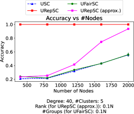
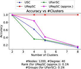
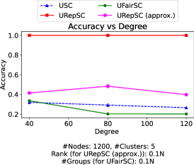
We sampled similarity graphs from $\mathcal{R}$-PP using $p=0.4$, $q=0.3$, $r=0.2$, and $s=0.1$ for various values of $d$, $N$, and $K$, while ensuring that the underlying $\mathcal{R}$ satisfies Assumption 4.1 and $\mathrm{rank}\{\mathbf{R}\}\leq N-k$. Figure 1 compares URepSC with unnormalized spectral clustering (USC) (Algorithm 1) and UFairSC. Figure 1a shows the effect of varying $N$ for a fixed $d=40$ and $K=5$. Figure 1b varies $K$ and keeps $N=1200$ and $d=40$ fixed. Similarly, Figure 1c keeps $N=1200$ and $K=5$ fixed and varies $d$. In all cases, we use $R=P=N/10$. The figures plot the accuracy on $y$-axis and report the mean and standard deviation across $10$ independent executions. As the ground truth clusters satisfy Definition 3.1 by construction, a high accuracy implies that the algorithm returns representation-aware clusters. In Figure 1a, it appears that even USC will return representation-aware clusters for a large enough graph. However, this is not true if the number of clusters increases with $N$ (Figure 1b), as is common in practice.

(a)

(b)

Figure 2: Comparing URepSC (approx.) with UFairSC using synthetically generated representation graphs sampled from an SBM.

Representation graphs sampled from planted partition model:

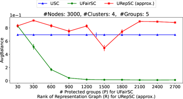
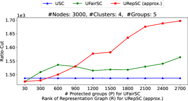
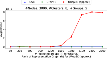
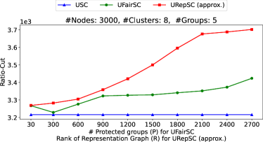
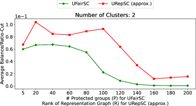
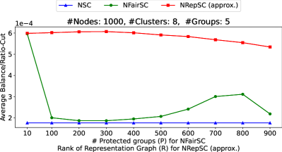
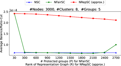
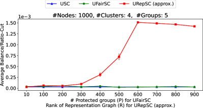
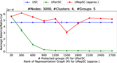
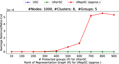
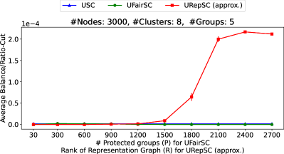
We divide the nodes into $P=5$ protected groups and sample a representation graph $\mathcal{R}$ using a (traditional) planted partition model with within (resp. across) protected group(s) connection probability given by $p_{\mathrm{in}}=0.8$ (resp. $p_{\mathrm{out}}=0.2$). Conditioned on $\mathcal{R}$, we then sample similarity graphs from $\mathcal{R}$-PP using the same parameters as before. We only experiment with URepSC (approx.) as an $\mathcal{R}$ generated this way may violate the rank assumption. Moreover, because such an $\mathcal{R}$ may not be $d$-regular, high accuracy no longer implies representation awareness, and we instead report the ratio of average individual balance $\bar{\rho}=\frac{1}{N}\sum_{i=1}^{N}\rho_{i}$ (see (3)) to the value of $\mathrm{RCut}$ in Figure 2. Higher values indicate high quality clusters that are also balanced from the perspective of individuals. Figure 2 shows a trade-off between accuracy and representation awareness. One can choose an appropriate value of $R$ in URepSC (approx.) to get good quality clusters with a high balance.

(a)

(b)

Figure 3: Comparing URepSC (approx.) with UFairSC on FAO trade network.

A real-world network:

The FAO trade network from United Nations is a multiplex network with $214$ nodes representing countries and $364$ layers representing commodities like coffee and barley (Domenico et al., 2015). Edges corresponding to the volume of trade between countries. We connect each node to its five nearest neighbors in each layer and make the edges undirected. The first $182$ layers are aggregated to construct $\mathcal{R}$ (connecting nodes that are connected in at least one layer) and the next $182$ layers are used for constructing $\mathcal{G}$. Note that $\mathcal{R}$ constructed this way is not $d$-regular. To motivate this experiment further, note that clusters based only on $\mathcal{G}$ only consider the trade of commodities $183$–$364$. However, countries also have other trade relations in $\mathcal{R}$, leading to shared economic interests. If the members of each cluster jointly formulate their economic policies, countries have an incentive to influence the economic policies of all clusters by having their representatives in them.

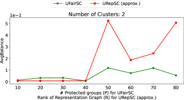
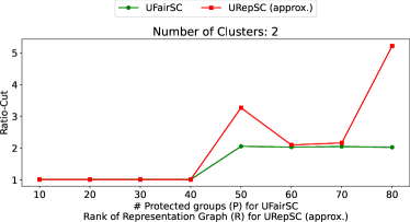
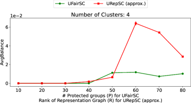
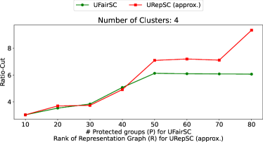
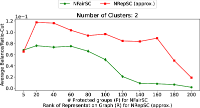
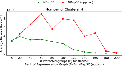
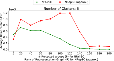
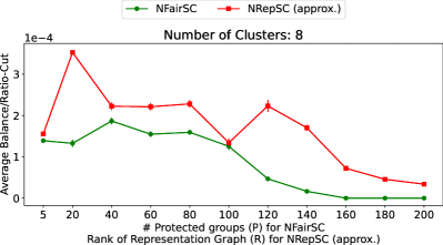
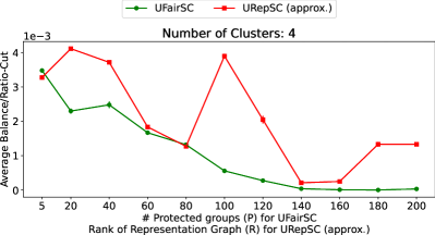
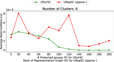
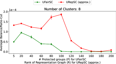
As before, we use the low-rank approximation for the representation graph in URepSC (approx.). Figure 3 compares URepSC (approx.) with UFairSC and has the same semantics as Figure 2. Different plots in Figure 3 correspond to different choices of $K$. URepSC (approx.) achieves a higher ratio of average balance to ratio-cut. In practice, a user would choose $R$ by assessing the relative importance of a quality metric like ratio-cut and representation metric like average balance.

Appendix F contains results for NRepSC, experiments with another real-world network, a few additional experiments related to URepSC, and a numerical validation of our time-complexity analysis. Appendix G contains plots that show both average balance and ratio-cut instead of their ratio.

6 Conclusion

We studied the consistency of constrained spectral clustering under a new individual level fairness constraint, called the representation constraint, using a novel $\mathcal{R}$-PP random graph model. Our work naturally generalizes existing population level constraints (Chierichetti et al., 2017) and associated spectral algorithms (Kleindessner et al., 2019). Four important avenues for future work include (i) the relaxation of the $d$-regularity assumption in our analysis (needed to ensure representation awareness of ground-truth clusters), (ii) better theoretical understanding of URepSC (approx.), (iii) improvement of the computational complexity of our algorithms, and (iv) exploring relaxed variants of our constraint and other (possibly non-spectral) algorithms for finding representation-aware clusters under such a relaxed constraint.

(a)

(b)

(c)

Figure 4: An example representation graph $\mathcal{R}$. Panel (a) shows the protected groups recovered from $\mathcal{R}$. Panel (b) shows the clusters recovered by a statistically fair clustering algorithm. Panel (c) shows the ideal individually fair clusters. (Best viewed in color)

Appendix A Representation constraint: Additional details

In this section, we make three additional remarks about the properties of the proposed constraint.

Need for individual fairness:

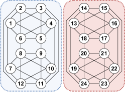
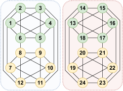
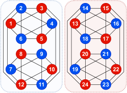
To understand the need for individual fairness notions, consider the representation graph $\mathcal{R}$ specified in Figure 4a. All the nodes have a self-loop associated with them that has not been shown for clarity. In this example, $N=24$, $K=2$, and every node is connected to $d=6$ nodes (including the self-loop). To use a statistical fairness notion [Chierichetti et al., 2017], one would begin by clustering the nodes in $\mathcal{R}$ to approximate the protected groups as the members of these protected groups will be each other’s representatives to the first order of approximation. A natural choice is to have two protected groups, as shown in Figure 4a using different colors. However, clustering nodes based on these protected groups can produce the green and yellow clusters shown in Figure 4b. It is easy to verify that these clusters satisfy the statistical fairness criterion as they have an equal number of members from both protected groups. However, these clusters are very "unfair" from the perspective of each individual. For example, node $v_{1}$ does not have enough representation in the yellow cluster as only one of its six representatives is in this cluster, despite the equal size of both the clusters. A similar argument can be made for every other node in this graph. This example highlights an extreme case where a statistically fair clustering is highly unfair from the perspective of each individual. Figure 4c shows another clustering assignment and it is easy to verify that each node in this assignment has the same representation in both red and blue clusters, making it individually fair with respect to $\mathcal{R}$. Our goal is to develop algorithms that prefer the clusters in Figure 4c over the clusters in Figure 4b.

Statistical fairness as a special case:

Recall that our constraint specifies an individual fairness notion. Contrast this with several existing approaches that assign each node to one of the $P$ protected groups $\mathcal{P}_{1},\dots,\mathcal{P}_{P}\subseteq\mathcal{V}$ [Chierichetti et al., 2017] and require these protected groups to have a proportional representation in all clusters, i.e.,

$$\frac{|\mathcal{P}_{i}\cap\mathcal{C}_{j}|}{|\mathcal{C}_{j}|}=\frac{|\mathcal{P}_{i}|}{N},\,\,\forall i\in[P],\,\,j\in[K].$$

This is an example of statistical fairness. In the previous paragraph, we argued that statistical fairness may not be enough in some cases. We now show that the constraint in Definition 3.1 is equivalent to a statistical fairness notion for an appropriately constructed representation graph $\mathcal{R}$ from the given protected groups $\mathcal{P}_{1},\dots,\mathcal{P}_{P}$. Namely, let $\mathcal{R}$ be such that $R_{ij}=1$ if and only if $v_{i}$ and $v_{j}$ belong to the same protected group. In this case, it is easy to verify that the constraint in Definition 3.1 reduces to the statistical fairness criterion given above. In general, for other configurations of the representation graph, we strictly generalize the statistical fairness notion. We also strictly generalize the approach presented in Kleindessner et al. [2019], where the authors use spectral clustering to produce statistically fair clusters. Also noteworthy is the assumption made by statistical fairness, namely that every pair of vertices in a protected group can represent each others’ interests ($R_{ij}=1\Leftrightarrow v_{i}$ and $v_{j}$ are in the same protected group) or they are very similar with respect to some sensitive attributes. This assumption becomes unreasonable as protected groups grow in size.

Sensitive attributes and protected groups:

Viewed as a fairness notion, the proposed constraint only requires a representation graph $\mathcal{R}$. It has two advantages over existing fairness criteria: (i) it does not require observable sensitive attributes (such as age, gender, and sexual orientation), and (ii) even if sensitive attributes are provided, one need not specify the number of protected groups or explicitly compute them. This ensures data privacy and helps against individual profiling. Our constraint only requires access to the representation graph $\mathcal{R}$. This graph can either be directly elicited from the individuals or derived as a function of several sensitive attributes. In either case, once $\mathcal{R}$ is available, we no longer need to expose any sensitive attributes to the clustering algorithm. For example, individuals in $\mathcal{R}$ may be connected if their age difference is less than five years and if they went to the same school. Crucially, the sensitive attributes used to construct $\mathcal{R}$ may be numerical, binary, categorical, etc.

Appendix B Normalized variant of the algorithm

Section B.1 presents the normalized variant of the traditional spectral clustering algorithm. Section B.2 describes our algorithm.

B.1 Normalized spectral clustering

The ratio-cut objective divides $\mathrm{Cut}(\mathcal{C}_{i},\mathcal{V}\backslash\mathcal{C}_{i})$ by the number of nodes in $\mathcal{C}_{i}$ to balance the size of the clusters. The volume of a cluster $\mathcal{C}\subseteq\mathcal{V}$, defined as $\mathrm{Vol}(\mathcal{C})=\sum_{v_{i}\in\mathcal{C}}D_{ii}$, is another popular notion of its size. The normalized cut or $\mathrm{NCut}$ objective divides $\mathrm{Cut}(\mathcal{C}_{i},\mathcal{V}\backslash\mathcal{C}_{i})$ by $\mathrm{Vol}(\mathcal{C}_{i})$, and is defined as

$$\mathrm{NCut}(\mathcal{C}_{1},\dots,\mathcal{C}_{K})=\sum_{i=1}^{K}\frac{\mathrm{Cut}(\mathcal{C}_{i},\mathcal{V}\backslash\mathcal{C}_{i})}{\mathrm{Vol}(\mathcal{C}_{i})}.$$

As before, one can show that $\mathrm{NCut}(\mathcal{C}_{1},\dots,\mathcal{C}_{K})=\mathrm{trace}\{\mathbf{T}^{\intercal}\mathbf{L}\mathbf{T}\}$ [von Luxburg, 2007], where $\mathbf{T}\in\mathbb{R}^{N\times K}$ is specified below.

$$T_{ij}=\begin{cases}\frac{1}{\sqrt{\mathrm{Vol}(\mathcal{C}_{j})}}&\text{ if }v_{i}\in\mathcal{C}_{j}\\ 0&\text{ otherwise.}\end{cases}$$ (10)

Note that $\mathbf{T}^{\intercal}\mathbf{D}\mathbf{T}=\mathbf{I}$. Thus, the optimization problem for minimizing the NCut objective is

$$\min_{\mathbf{T}\in\mathbb{R}^{N\times K}}\,\,\,\,\mathrm{trace}\{\mathbf{T}^{\intercal}\mathbf{L}\mathbf{T}\}\,\,\,\,\text{s.t.}\,\,\,\,\mathbf{T}^{\intercal}\mathbf{D}\mathbf{T}=\mathbf{I}\text{ and }\mathbf{T}\text{ is of the form \eqref{eq:T_def}.}$$ (11)

As before, this optimization problem is hard to solve, and normalized spectral clustering solves a relaxed variant of this problem. Let $\mathbf{H}=\mathbf{D}^{1/2}\mathbf{T}$ and define the normalized graph Laplacian as $\mathbf{L}_{\mathrm{norm}}=\mathbf{I}-\mathbf{D}^{-1/2}\mathbf{A}\mathbf{D}^{-1/2}$. Normalized spectral clustering solves the following relaxed problem:

$$\min_{\mathbf{H}\in\mathbb{R}^{N\times K}}\,\,\,\,\mathrm{trace}\{\mathbf{H}^{\intercal}\mathbf{L}_{\mathrm{norm}}\mathbf{H}\}\,\,\,\,\text{s.t.}\,\,\,\,\mathbf{H}^{\intercal}\mathbf{H}=\mathbf{I}.$$ (12)

Note that $\mathbf{H}^{\intercal}\mathbf{H}=\mathbf{I}\Leftrightarrow\mathbf{T}^{\intercal}\mathbf{D}\mathbf{T}=\mathbf{I}$. This is again the standard form of the trace minimization problem that can be solved using the Rayleigh-Ritz theorem. Algorithm 3 summarizes the normalized spectral clustering algorithm.

1:Input: Adjacency matrix $\mathbf{A}$, number of clusters $K\geq 2$

2:Compute the normalized Laplacian matrix $\mathbf{L}_{\mathrm{norm}}=\mathbf{I}-\mathbf{D}^{-1/2}\mathbf{A}\mathbf{D}^{-1/2}$.

3:Compute the first $K$ eigenvectors $\mathbf{u}_{1},\dots,\mathbf{u}_{K}$ of $\mathbf{L}_{\mathrm{norm}}$. Let $\mathbf{H}^{*}\in\mathbb{R}^{N\times K}$ be a matrix that has $\mathbf{u}_{1},\dots,\mathbf{u}_{K}$ as its columns.

4:Let $\mathbf{h}^{*}_{i}$ denote the $i^{th}$ row of $\mathbf{H}^{*}$. Compute $\tilde{\mathbf{h}}^{*}_{i}=\frac{\mathbf{h}^{*}_{i}}{||\mathbf{h}^{*}_{i}||_{2}}$ for all $i=1,2,\dots,N$.

5:Cluster $\tilde{\mathbf{h}}^{*}_{1},\dots,\tilde{\mathbf{h}}^{*}_{N}$ into $K$ clusters using $k$-means clustering.

6:Output: Clusters $\hat{\mathcal{C}}_{1},\dots,\hat{\mathcal{C}}_{K}$, s.t. $\hat{\mathcal{C}}_{i}=\{v_{j}\in\mathcal{V}:\tilde{\mathbf{h}}^{*}_{j}\text{ was assigned to the }i^{th}\text{ cluster}\}$.

Algorithm 3 Normalized spectral clustering

B.2 Normalized representation-aware spectral clustering (NRepSC)

We use a similar strategy as in Section 3.2 to develop the normalized variant of our algorithm. Recall from Section B.1 that normalized spectral clustering approximately minimizes the $\mathrm{NCut}$ objective. The lemma below is a counterpart of Lemma 3.1. It formulates a sufficient condition that implies our constraint in (5), but this time in terms of the matrix $\mathbf{T}$ defined in (10).

Lemma B.1.

Let $\mathbf{T}\in\mathbb{R}^{N\times K}$ have the form specified in (10). The condition

$$\mathbf{R}\left(\mathbf{I}-\frac{1}{N}\bm{1}\bm{1}^{\intercal}\right)\mathbf{T}=\mathbf{0}$$ (13)

implies that the corresponding clusters $\mathcal{C}_{1},\dots,\mathcal{C}_{K}$ satisfy (5). Here, $\mathbf{I}$ is the $N\times N$ identity matrix and $\bm{1}$ is a $N$ dimensional all-ones vector.

For NRepSC, we assume that the similarity graph $\mathcal{G}$ is connected so that the diagonal entries of $\mathbf{D}$ are strictly positive. We proceed as before to incorporate constraint (13) in optimization problem (11). After applying the spectral relaxation, we get

$$\min_{\mathbf{T}}\;\;\;\;\mathrm{trace}\{\mathbf{T}^{\intercal}\mathbf{L}\mathbf{T}\}\;\;\;\;\text{s.t.}\;\;\;\;\mathbf{T}^{\intercal}\mathbf{D}\mathbf{T}=\mathbf{I};\;\;\;\;\mathbf{R}(\mathbf{I}-\bm{1}\bm{1}^{\intercal}/N)\mathbf{T}=\mathbf{0}.$$ (14)

As before, $\mathbf{T}=\mathbf{Y}\mathbf{Z}$ for some $\mathbf{Z}\in\mathbb{R}^{N-r\times K}$, where recall that columns of $\mathbf{Y}$ contain orthonormal basis for $\mathrm{null}\{\mathbf{R}(\mathbf{I}-\bm{1}\bm{1}^{\intercal}/N)\}$. This reparameterization yields

$$\min_{\mathbf{Z}}\;\;\;\;\mathrm{trace}\{\mathbf{Z}^{\intercal}\mathbf{Y}^{\intercal}\mathbf{L}\mathbf{Y}\mathbf{Z}\}\;\;\;\;\text{s.t.}\;\;\;\;\mathbf{Z}^{\intercal}\mathbf{Y}^{\intercal}\mathbf{D}\mathbf{Y}\mathbf{Z}=\mathbf{I}.$$

Define $\mathbf{Q}\in\mathbb{R}^{N-r\times N-r}$ such that $\mathbf{Q}^{2}=\mathbf{Y}^{\intercal}\mathbf{D}\mathbf{Y}$. Note that $\mathbf{Q}$ exists as the entries of $\mathbf{D}$ are non-negative. Let $\mathbf{V}=\mathbf{Q}\mathbf{Z}$. Then, $\mathbf{Z}=\mathbf{Q}^{-1}\mathbf{V}$ and $\mathbf{Z}^{\intercal}\mathbf{Q}^{2}\mathbf{Z}=\mathbf{V}^{\intercal}\mathbf{V}$ as $\mathbf{Q}$ is symmetric. Reparameterizing again, we get

$$\min_{\mathbf{V}}\;\;\;\;\mathrm{trace}\{\mathbf{V}^{\intercal}\mathbf{Q}^{-1}\mathbf{Y}^{\intercal}\mathbf{L}\mathbf{Y}\mathbf{Q}^{-1}\mathbf{V}\}\;\;\;\;\text{s.t.}\;\;\;\;\mathbf{V}^{\intercal}\mathbf{V}=\mathbf{I}.$$

This again is the standard form of the trace minimization problem and the optimal solution is given by the leading $K$ eigenvectors of $\mathbf{Q}^{-1}\mathbf{Y}^{\intercal}\mathbf{L}\mathbf{Y}\mathbf{Q}^{-1}$. Algorithm 4 summarizes the normalized representation-aware spectral clustering algorithm, which we denote by NRepSC. Note that the algorithm assumes that $\mathbf{Q}$ is invertible, which requires the absence of isolated nodes in the similarity graph $\mathcal{G}$.

1:Input: Adjacency matrix $\mathbf{A}$, representation graph $\mathbf{R}$, number of clusters $K\geq 2$

2:Compute $\mathbf{Y}$ containing orthonormal basis vectors of $\mathrm{null}\{\mathbf{R}(\mathbf{I}-\frac{1}{N}\bm{1}\bm{1}^{\intercal})\}$

3:Compute Laplacian $\mathbf{L}=\mathbf{D}-\mathbf{A}$

4:Compute $\mathbf{Q}=\sqrt{\mathbf{Y}^{\intercal}\mathbf{D}\mathbf{Y}}$ using the matrix square root

5:Compute leading $K$ eigenvectors of $\mathbf{Q}^{-1}\mathbf{Y}^{\intercal}\mathbf{L}\mathbf{Y}\mathbf{Q}^{-1}$. Set them as columns of $\mathbf{V}\in\mathbb{R}^{N-r\times K}$

6:Apply $k$-means clustering to the rows of $\mathbf{T}=\mathbf{Y}\mathbf{Q}^{-1}\mathbf{V}$ to get clusters $\hat{\mathcal{C}}_{1},\hat{\mathcal{C}}_{2},\dots,\hat{\mathcal{C}}_{K}$

7:Return: Clusters $\hat{\mathcal{C}}_{1},\hat{\mathcal{C}}_{2},\dots,\hat{\mathcal{C}}_{K}$

Algorithm 4 NRepSC

Appendix C A note on the approximate variants of our algorithms

Recall the URepSC (approx.) algorithm from Section 3.2 that we use in our experiments when $\mathrm{rank}\{\mathbf{R}\}>N-K$. It first obtains a rank $R\leq N-K$ approximation of $\mathbf{R}$ and then uses the approximate $\mathbf{R}$ in Algorithm 1. NRepSC (approx.) can be analogously defined for NRepSC in Algorithm 4. In this section, we provide additional intuition behind this idea of using a low rank approximation of $\mathbf{R}$.

Existing (population-level) fairness notions for clustering assign a categorical value to each node and treat it as its sensitive attribute. Based on this sensitive attribute, the set of nodes $\mathcal{V}$ can be partitioned into $P$ protected groups $\mathcal{P}_{1},\dots,\mathcal{P}_{P}\subseteq\mathcal{V}$ such that all nodes in $\mathcal{P}_{i}$ have the $i^{th}$ value for the sensitive attribute. Our guiding motivation behind representation graph was to connect nodes in $\mathcal{R}$ based on their similarity with respect to multiple sensitive attributes of different types (see Section 3.1). Finding clusters in $\mathcal{R}$ is then in the same spirit as clustering the original sensitive attributes and approximating their combined effect via a single categorical meta-sensitive attribute (the cluster to which the node belongs in $\mathcal{R}$). Indeed, as described in Section 5, we do this while experimenting with UFairSC and NFairSC from Kleindessner et al. [2019] in our experiments.

Appendix A shows that a block diagonal $\mathbf{R}$ encodes protected groups $\mathcal{P}_{1},\dots,\mathcal{P}_{P}$ defined above and reduces our representation constraint to the existing population level constraint [Chierichetti et al., 2017], thereby recovering all existing results from Kleindessner et al. [2019] as a special case of our analysis. A natural question to ask is how a low rank approximation of $\mathbf{R}$ is different from the block diagonal matrix described in Appendix A and why the approximate variants of URepSC and NRepSC are different from simply using UFairSC and NFairSC on clusters in $\mathcal{R}$, as described in Section 5.

To understand the differences, first note that a low rank approximation $\hat{\mathbf{R}}$ of $\mathbf{R}$ need not have a block diagonal structure with only ones and zeros. Entry $\hat{R}_{ij}$ approximates the strength of similarity between nodes $i$ and $j$. The constraint $\hat{\mathbf{R}}(\mathbf{I}-\bf 1\bf 1^{\intercal}/N)$ translates to

$$\sum_{j=1}^{N}\hat{R}_{ij}H_{jk}=\frac{1}{N}\left(\sum_{j=1}^{N}\hat{R}_{ij}\right)\left(\sum_{j=1}^{N}H_{jk}\right),\;\;\;\;\forall i\in[N],k\in[K].$$

Let us look at a particular node $v_{i}$ and focus on a particular cluster $\mathcal{C}_{k}$. If $\mathbf{H}$ has the form specified in (1), we get

$$\frac{1}{|\mathcal{C}_{k}|}\sum_{j:v_{j}\in\mathcal{C}_{k}}\hat{R}_{ij}=\frac{1}{N}\sum_{j=1}^{N}\hat{R}_{ij}.$$

From the perspective of node $v_{i}$, this constraint requires the average similarity of $v_{i}$ to other nodes in $\mathcal{C}_{k}$ to be same as the average similarity of node $v_{i}$ to all other nodes in the population. This must simultaneously hold for all clusters $\mathcal{C}_{k}$ so that nodes similar to $v_{i}$ are present on an average in all clusters. One can see this as a continuous variant of our constraint in Definition 3.1.

An important point to note is that this is still an individual level constraint and reduces to the existing population level constraint only when $\hat{\mathbf{R}}$ is binary and block diagonal (Appendix A). Thus, in general, using a low rank approximation of $\mathbf{R}$ is different from first clustering $\mathbf{R}$ and then using the resulting protected groups in UFairSC and NFairSC. Therefore, URepSC (approx.) and NRepSC (approx.) do not trivially reduce to UFairSC and NFairSC from Kleindessner et al. [2019]. This is clearly visible in our experiments where the approximate variants perform better in terms of individual balance as compared to UFairSC and NFairSC.

Unfortunately, defining $\mathcal{R}$-PP for an $\mathcal{R}$ with continuous valued entries is not straightforward. This makes the analysis of the approximate variants more challenging. However, we believe that their practical utility outweighs the lack of theoretical guarantees and leave such an analysis for future work.

Appendix D Proof of Theorems 4.1 and 4.2

The proof of Theorems 4.1 and 4.2 follow the commonly used template for such results [Rohe et al., 2011, Lei and Rinaldo, 2015]. In the context of URepSC (similar arguments work for NRepSC as well), we

1. Compute the expected Laplacian matrix $\mathcal{L}$ under $\mathcal{R}$-PP and show that its top $K$ eigenvectors can be used to recover the ground-truth clusters (Lemmas D.1–D.3).

2. Show that these top $K$ eigenvectors lie in the null space of $\mathbf{R}(\mathbf{I}-\bm{1}\bm{1}^{\intercal}/N)$ and hence are also the top $K$ eigenvectors of $\mathbf{Y}^{\intercal}\mathcal{L}\mathbf{Y}$ (Lemma D.4). This implies that Algorithm 2 returns the ground truth clusters in the expected case.

3. Use matrix perturbation arguments to establish a high probability mistake bound in the general case when the graph $\mathcal{G}$ is sampled from a $\mathcal{R}$-PP (Lemmas D.5–D.8).

We begin with a series of lemmas that highlight certain useful properties of eigenvalues and eigenvectors of the expected Laplacian $\mathcal{L}$. These lemmas will be used in Sections D.1 and D.2 to prove Theorems 4.1 and 4.2, respectively. See Appendix E for the proofs of all technical lemmas. For the remainder of this section, we assume that all appropriate assumptions made in Theorems 4.1 and 4.2 are satisfied.

The first lemma shows that certain vectors that can be used to recover the ground-truth clusters indeed satisfy the representation constraint in (6) and (13).

Lemma D.1.

The $N$-dimensional vector of all ones, denoted by $\bm{1}$, is an eigenvector of $\mathbf{R}$ with eigenvalue $d$. Define $\mathbf{u}_{k}\in\mathbb{R}^{N}$ for $k\in[K-1]$ as,

$$u_{ki}=\begin{cases}1&\text{ if }v_{i}\in\mathcal{C}_{k}\\ -\frac{1}{K-1}&\text{ otherwise,}\end{cases}$$

where $u_{ki}$ is the $i^{th}$ element of $\mathbf{u}_{k}$. Then, $\bm{1},\mathbf{u}_{1},\dots,\mathbf{u}_{K-1}\in\mathrm{null}\{\mathbf{R}(\mathbf{I}-\frac{1}{N}\bm{1}\bm{1}^{\intercal})\}$. Moreover, $\bm{1},\mathbf{u}_{1},\dots,\mathbf{u}_{K-1}$ are linearly independent.

Recall that we use $\mathcal{A}\in\mathbb{R}^{N\times N}$ to denote the expected adjacency matrix of the similarity graph $\mathcal{G}$. Clearly, $\mathcal{A}=\tilde{\mathcal{A}}-p\mathbf{I}$, where $\tilde{\mathcal{A}}$ is such that $\tilde{\mathcal{A}}_{ij}=P(A_{ij}=1)$ if $i\neq j$ (see (9)) and $\tilde{\mathcal{A}}_{ii}=p$ otherwise. Note that

$$\tilde{\mathcal{A}}\mathbf{x}=\lambda\mathbf{x}\,\,\,\,\Leftrightarrow\,\,\,\,\mathcal{A}\mathbf{x}=(\lambda-p)\mathbf{x}.$$ (15)

Simple algebra shows that $\tilde{\mathcal{A}}$ can be written as

$$\tilde{\mathcal{A}}=q\mathbf{R}+s(\bm{1}\bm{1}^{\intercal}-\mathbf{R})+(p-q)\sum_{k=1}^{K}\mathbf{G}_{k}\mathbf{R}\mathbf{G}_{k}+(r-s)\sum_{k=1}^{K}\mathbf{G}_{k}(\bm{1}\bm{1}^{\intercal}-\mathbf{R})\mathbf{G}_{k},$$ (16)

where, for all $k\in[K]$, $\mathbf{G}_{k}\in\mathbb{R}^{N\times N}$ is a diagonal matrix such that $(\mathbf{G}_{k})_{ii}=1$ if $v_{i}\in\mathcal{C}_{k}$ and $0$ otherwise. The next lemma shows that $\bm{1},\mathbf{u}_{1},\dots,\mathbf{u}_{K-1}$ defined in Lemma D.1 are eigenvectors of $\tilde{\mathcal{A}}$.

Lemma D.2.

Let $\bm{1},\mathbf{u}_{1},\dots,\mathbf{u}_{K-1}$ be as defined in Lemma D.1. Then,

$$\tilde{\mathcal{A}}\bm{1} = \lambda_{1}\bm{1}\text{ where }\lambda_{1}=qd+s(N-d)+(p-q)\frac{d}{K}+(r-s)\frac{N-d}{K},\text{ and }$$

$$\tilde{\mathcal{A}}\mathbf{u}_{k} = \lambda_{1+k}\mathbf{u}_{k}\text{ where }\lambda_{1+k}=(p-q)\frac{d}{K}+(r-s)\frac{N-d}{K}.$$

Let $\mathcal{L}=\mathcal{D}-\mathcal{A}$ be the expected Laplacian matrix, where $\mathcal{D}$ is a diagonal matrix with $\mathcal{D}_{ii}=\sum_{j=1}^{N}\mathcal{A}_{ij}$ for all $i\in[N]$. It is easy to see that $\mathcal{D}_{ii}=\lambda_{1}-p$ for all $i\in[N]$ as $\mathcal{A}\bm{1}=(\lambda_{1}-p)\bm{1}$ by (15) and Lemma D.2. Thus, $\mathcal{D}=(\lambda_{1}-p)\mathbf{I}$ and hence any eigenvector of $\tilde{\mathcal{A}}$ with eigenvalue $\lambda$ is also an eigenvector of $\mathcal{L}$ with eigenvalue $\lambda_{1}-\lambda$. That is, if $\tilde{\mathcal{A}}\mathbf{x}=\lambda\mathbf{x}$,

$$\mathcal{L}\mathbf{x}=(\mathcal{D}-\mathcal{A})\mathbf{x}=((\lambda_{1}-p)\mathbf{I}-(\tilde{\mathcal{A}}-p\mathbf{I}))\mathbf{x}=(\lambda_{1}-\lambda)\mathbf{x}.$$ (17)

Hence, the eigenvectors of $\mathcal{L}$ corresponding to the $K$ smallest eigenvalues are the same as the eigenvectors of $\tilde{\mathcal{A}}$ corresponding to the $K$ largest eigenvalues.

Recall that the columns of the matrix $\mathbf{Y}$ used in Algorithms 2 and 4 contain the orthonormal basis for the null space of $\mathbf{R}(\mathbf{I}-\bm{1}\bm{1}^{\intercal}/N)$. To solve (8) and (14), we only need to optimize over vectors that belong to this null space. By Lemma D.1, $\bm{1},\mathbf{u}_{1},\dots,\mathbf{u}_{K-1}\in\mathrm{null}\{\mathbf{R}(\mathbf{I}-\bm{1}\bm{1}^{\intercal}/N)\}$ and these vectors are linearly independent. However, we need an orthonormal basis to compute $\mathbf{Y}$. Let $\mathbf{y}_{1}=\bm{1}/\sqrt{N}$ and $\mathbf{y}_{2},\dots,\mathbf{y}_{K}$ be orthonormal vectors that span the same space as $\mathbf{u}_{1},\dots,\mathbf{u}_{K-1}$. The next lemma computes such $\mathbf{y}_{2},\dots,\mathbf{y}_{K}$. The matrix $\mathbf{Y}\in\mathbb{R}^{N\times N-r}$ contains these vectors $\mathbf{y}_{1},\dots,\mathbf{y}_{K}$ as its first $K$ columns.

Lemma D.3.

Define $\mathbf{y}_{1+k}\in\mathbb{R}^{N}$ for $k\in[K-1]$ as

$$y_{1+k,i}=\begin{cases}0&\text{ if }v_{i}\in\mathcal{C}_{k{{}^{\prime}}}\text{ s.t. }k{{}^{\prime}}<k\\ \frac{K-k}{\sqrt{\frac{N}{K}(K-k)(K-k+1)}}&\text{ if }v_{i}\in\mathcal{C}_{k}\\ -\frac{1}{\sqrt{\frac{N}{K}(K-k)(K-k+1)}}&\text{ otherwise.}\end{cases}$$

Then, for all $k\in[K-1]$, $\mathbf{y}_{1+k}$ are orthonormal vectors that span the same space as $\mathbf{u}_{1},\mathbf{u}_{2},\dots,\mathbf{u}_{K-1}$ and $\mathbf{y}_{1}^{\intercal}\mathbf{y}_{1+k}=0$. As before, $y_{1+k,i}$ refers to the $i^{th}$ element of $\mathbf{y}_{1+k}$.

Let $\mathbf{X}\in\mathbb{R}^{N\times K}$ be such that it has $\mathbf{y}_{1},\dots,\mathbf{y}_{K}$ as its columns. If two nodes belong to the same cluster, the rows corresponding to these nodes in $\mathbf{X}\mathbf{U}$ will be identical for any $\mathbf{U}\in\mathbb{R}^{K\times K}$ such that $\mathbf{U}^{\intercal}\mathbf{U}=\mathbf{U}\mathbf{U}^{\intercal}=\mathbf{I}$. Thus, any $K$ orthonormal vectors belonging to the span of $\mathbf{y}_{1},\dots,\mathbf{y}_{K}$ can be used to recover the ground truth clusters. With the general properties of the eigenvectors and eigenvalues established in the lemmas above, we next move on to the proof of Theorem 4.1 in the next section and Theorem 4.2 in Section D.2.

D.1 Proof of Theorem 4.1

Let $\mathcal{Z}\in\mathbb{R}^{N-r\times K}$ be a solution to the optimization problem (8) in the expected case with $\mathcal{A}$ as input. The next lemma shows that columns of $\mathbf{Y}\mathcal{Z}$ indeed lie in the span of $\mathbf{y}_{1},\dots,\mathbf{y}_{K}$. Thus, the $k$-means clustering step in Algorithm 2 will return the correct ground truth clusters when $\mathcal{A}$ is passed as input.

Lemma D.4.

Let $\mathbf{y}_{1}=\bm{1}/\sqrt{N}$ and $\mathbf{y}_{1+k}$ be as defined in Lemma D.3 for all $k\in[K-1]$. Further, let $\mathcal{Z}$ be the optimal solution of the optimization problem in (8) with $\mathbf{L}$ set to $\mathcal{L}$. Then, the columns of $\mathbf{Y}\mathcal{Z}$ lie in the span of $\mathbf{y}_{1},\mathbf{y}_{2},\dots,\mathbf{y}_{K}$.

Next, we use arguments from matrix perturbation theory to show a high-probability bound on the number of mistakes made by the algorithm. In particular, we need an upper bound on $||\mathbf{Y}^{\intercal}\mathbf{L}\mathbf{Y}-\mathbf{Y}^{\intercal}\mathcal{L}\mathbf{Y}||$, where $\mathbf{L}$ is the Laplacian matrix for a graph randomly sampled from $\mathcal{R}$-PP and $||\mathbf{P}||=\sqrt{\lambda_{\max}(\mathbf{P}^{\intercal}\mathbf{P})}$ for any matrix $\mathbf{P}$. Note that $||\mathbf{Y}||=||\mathbf{Y}^{\intercal}||=1$ as $\mathbf{Y}^{\intercal}\mathbf{Y}=\mathbf{I}$. Thus,

$$||\mathbf{Y}^{\intercal}\mathbf{L}\mathbf{Y}-\mathbf{Y}^{\intercal}\mathcal{L}\mathbf{Y}||\leq||\mathbf{Y}^{\intercal}||\,\,||\mathbf{L}-\mathcal{L}||\,\,||\mathbf{Y}||=||\mathbf{L}-\mathcal{L}||.$$ (18)

Moreover,

$$||\mathbf{L}-\mathcal{L}||=||\mathbf{D}-\mathbf{A}-(\mathcal{D}-\mathcal{A})||\leq||\mathbf{D}-\mathcal{D}||+||\mathbf{A}-\mathcal{A}||.$$

The next two lemmas bound the two terms on the right hand side of the inequality above, thus providing an upper bound on $||\mathbf{L}-\mathcal{L}||$ and hence on $||\mathbf{Y}^{\intercal}\mathbf{L}\mathbf{Y}-\mathbf{Y}^{\intercal}\mathcal{L}\mathbf{Y}||$ by (18).

Lemma D.5.

Assume that $p\geq C\frac{\ln N}{N}$ for some constant $C>0$. Then, for every $\alpha>0$, there exists a constant $\mathrm{const}_{1}(C,\alpha)$ that only depends on $C$ and $\alpha$ such that

$$||\mathbf{D}-\mathcal{D}||\leq\mathrm{const}_{1}(C,\alpha)\sqrt{pN\ln N}$$

with probability at-least $1-N^{-\alpha}$.

Lemma D.6.

Assume that $p\geq C\frac{\ln N}{N}$ for some constant $C>0$. Then, for every $\alpha>0$, there exists a constant $\mathrm{const}_{4}(C,\alpha)$ that only depends on $C$ and $\alpha$ such that

$$||\mathbf{A}-\mathcal{A}||\leq\mathrm{const}_{4}(C,\alpha)\sqrt{pN}$$

with probability at-least $1-N^{-\alpha}$.

From Lemmas D.5 and D.6, we conclude that there is always a constant $\mathrm{const}_{5}(C,\alpha)=\max\{\mathrm{const}_{1}(C,\alpha),\mathrm{const}_{4}(C,\alpha)\}$ such that for any $\alpha>0$, with probability at least $1-2N^{-\alpha}$,

$$||\mathbf{Y}^{\intercal}\mathbf{L}\mathbf{Y}-\mathbf{Y}^{\intercal}\mathcal{L}\mathbf{Y}||\leq||\mathbf{L}-\mathcal{L}||\leq\mathrm{const}_{5}(C,\alpha)\sqrt{pN\ln N}.$$ (19)

Let $\mathcal{Z}$ and $\mathbf{Z}$ denote the optimal solution of (8) in the expected ($\mathbf{L}$ replaced with $\mathcal{L}$) and observed case. We use (19) to show a bound on $||\mathbf{Y}\mathcal{Z}-\mathbf{Y}Z||_{F}$ in Lemma D.7 and then use this bound to argue that Algorithm 2 makes a small number of mistakes when the graph is sampled from $\mathcal{R}$-PP.

Lemma D.7.

Let $\mu_{1}\leq\mu_{2}\leq\dots\leq\mu_{N-r}$ be eigenvalues of $\mathbf{Y}^{\intercal}\mathcal{L}\mathbf{Y}$. Further, let the columns of $\mathcal{Z}\in\mathbb{R}^{N-r\times K}$ and $\mathbf{Z}\in\mathbb{R}^{N-r\times K}$ correspond to the leading $K$ eigenvectors of $\mathbf{Y}^{\intercal}\mathcal{L}\mathbf{Y}$ and $\mathbf{Y}^{\intercal}\mathbf{L}\mathbf{Y}$, respectively. Define $\gamma=\mu_{K+1}-\mu_{K}$. Then, with probability at least $1-2N^{-\alpha}$,

$$\inf_{\mathbf{U}\in\mathbb{R}^{K\times K}:\mathbf{U}\mathbf{U}^{\intercal}=\mathbf{U}^{\intercal}\mathbf{U}=\mathbf{I}}||\mathbf{Y}\mathcal{Z}-\mathbf{Y}\mathbf{Z}\mathbf{U}||_{F}\leq\mathrm{const}_{5}(C,\alpha)\frac{4\sqrt{2K}}{\gamma}\sqrt{pN\ln N},$$

where $\mathrm{const}_{5}(C,\alpha)$ is from (19).

Recall that $\mathbf{X}\in\mathbb{R}^{N\times K}$ is a matrix that contains $\mathbf{y}_{1},\dots,\mathbf{y}_{K}$ as its columns. Let $\mathbf{x}_{i}$ denote the $i^{th}$ row of $\mathbf{X}$. Simple calculation using Lemma D.3 shows that,

$$||\mathbf{x}_{i}-\mathbf{x}_{j}||_{2}=\begin{cases}0&\text{ if }v_{i}\text{ and }v_{j}\text{ belong to the same cluster}\\ \sqrt{\frac{2K}{N}}&\text{ otherwise.}\end{cases}$$

By Lemma D.4, $\mathcal{Z}$ can be chosen such that $\mathbf{Y}\mathcal{Z}=\mathbf{X}$. Let $\mathbf{U}$ be the matrix that solves $\inf_{\mathbf{U}\in\mathbb{R}^{K\times K}:\mathbf{U}\mathbf{U}^{\intercal}=\mathbf{U}^{\intercal}\mathbf{U}=\mathbf{I}}||\mathbf{Y}\mathcal{Z}-\mathbf{Y}\mathbf{Z}\mathbf{U}||_{F}$. As $\mathbf{U}$ is orthogonal, $||\mathbf{x}_{i}^{\intercal}\mathbf{U}-\mathbf{x}_{j}^{\intercal}\mathbf{U}||_{2}=||\mathbf{x}_{i}-\mathbf{x}_{j}||_{2}$. The following lemma is a direct consequence of Lemma 5.3 in Lei and Rinaldo [2015].

Lemma D.8.

Let $\mathbf{X}$ and $\mathbf{U}$ be as defined above. For any $\epsilon>0$, let $\hat{\bm{\Theta}}\in\mathbb{R}^{N\times K}$ be the assignment matrix returned by a $(1+\epsilon)$-approximate solution to the $k$-means clustering problem when rows of $\mathbf{Y}\mathbf{Z}$ are provided as input features. Further, let $\hat{\bm{\mu}}_{1}$, $\hat{\bm{\mu}}_{2}$, …, $\hat{\bm{\mu}}_{K}\in\mathbb{R}^{K}$ be the estimated cluster centroids. Define $\hat{\mathbf{X}}=\hat{\bm{\Theta}}\hat{\bm{\mu}}$ where $\hat{\bm{\mu}}\in\mathbb{R}^{K\times K}$ contains $\hat{\bm{\mu}}_{1},\dots,\hat{\bm{\mu}}_{K}$ as its rows. Further, define $\delta=\sqrt{\frac{2K}{N}}$, and $S_{k}=\{v_{i}\in\mathcal{C}_{k}:||\hat{\mathbf{x}}_{i}-\mathbf{x}_{i}||\geq\delta/2\}$. Then,

$$\delta^{2}\sum_{k=1}^{K}|S_{k}|\leq 8(2+\epsilon)||\mathbf{X}\mathbf{U}^{\intercal}-\mathbf{Y}\mathbf{Z}||_{F}^{2}.$$ (20)

Moreover, if $\gamma$ from Lemma D.7 satisfies $\gamma^{2}>\mathrm{const}(C,\alpha)(2+\epsilon)pNK\ln N$ for a universal constant $\mathrm{const}(C,\alpha)$, there exists a permutation matrix $\mathbf{J}\in\mathbb{R}^{K\times K}$ such that

$$\hat{\bm{\theta}}_{i}^{\intercal}\mathbf{J}=\bm{\theta}_{i}^{\intercal},\,\,\,\,\forall\,\,i\in[N]\backslash(\cup_{k=1}^{K}S_{k}).$$ (21)

Here, $\hat{\bm{\theta}}_{i}\mathbf{J}$ and $\bm{\theta}_{i}$ represent the $i^{th}$ row of matrix $\hat{\bm{\Theta}}\mathbf{J}$ and $\bm{\Theta}$ respectively.

By the definition of $M(\bm{\Theta},\hat{\bm{\Theta}})$, for the matrix $\mathbf{J}$ used in Lemma D.8, $M(\bm{\Theta},\hat{\bm{\Theta}})\leq\frac{1}{N}||\bm{\Theta}-\hat{\bm{\Theta}}\mathbf{J}||_{0}$. But, according to Lemma D.8, $||\bm{\Theta}-\hat{\bm{\Theta}}\mathbf{J}||_{0}\leq 2\sum_{k=1}^{K}|S_{k}|$. Using Lemmas D.7 and D.8, we get

$$M(\bm{\Theta},\hat{\bm{\Theta}})\leq\frac{1}{N}||\bm{\Theta}-\hat{\bm{\Theta}}\mathbf{J}||_{0}\leq\frac{2}{N}\sum_{k=1}^{K}|S_{k}| \leq \frac{16(2+\epsilon)}{N\delta^{2}}||\mathbf{X}\mathbf{U}^{\intercal}-\mathbf{Y}\mathbf{Z}||_{F}^{2}$$

$$\leq \mathrm{const}_{5}(C,\alpha)^{2}\frac{512(2+\epsilon)}{N\delta^{2}\gamma^{2}}pNK\ln N.$$

Noting that $\delta=\sqrt{\frac{2K}{N}}$ and setting $\mathrm{const}(C,\alpha)=256\times\mathrm{const}_{5}(C,\alpha)^{2}$ finishes the proof.

D.2 Proof of Theorem 4.2

Recall that $\mathbf{Q}=\sqrt{\mathbf{Y}^{\intercal}\mathbf{D}\mathbf{Y}}$ and analogously define $\mathcal{Q}=\sqrt{\mathbf{Y}^{\intercal}\mathcal{D}\mathbf{Y}}$, where $\mathcal{D}$ is the expected degree matrix. It was shown after Lemma D.2 that $\mathcal{D}=(\lambda_{1}-p)\mathbf{I}$. Thus, $\mathcal{Q}=\sqrt{\lambda_{1}-p}\;\mathbf{I}$ as $\mathbf{Y}^{\intercal}\mathbf{Y}=\mathbf{I}$. Hence $\mathcal{Q}^{-1}\mathbf{Y}^{\intercal}\mathcal{L}\mathbf{Y}\mathcal{Q}^{-1}=\frac{1}{\lambda_{1}-p}\mathbf{Y}^{\intercal}\mathcal{L}\mathbf{Y}$. Therefore, $\mathcal{Q}^{-1}\mathbf{Y}^{\intercal}\mathcal{L}\mathbf{Y}\mathcal{Q}^{-1}\mathbf{x}=\frac{\lambda}{\lambda_{1}-p}\mathbf{x}\;\Longleftrightarrow\;\mathbf{Y}^{\intercal}\mathcal{L}\mathbf{Y}\mathbf{x}=\lambda\mathbf{x}$. Let $\mathcal{Z}\in\mathbb{R}^{N-r\times K}$ contain the leading $K$ eigenvectors of $\mathcal{Q}^{-1}\mathbf{Y}^{\intercal}\mathcal{L}\mathbf{Y}\mathcal{Q}^{-1}$ as its columns. Algorithm 4 will cluster the rows of $\mathbf{Y}\mathcal{Q}^{-1}\mathcal{Z}$ to recover the clusters in the expected case. As $\mathcal{Q}^{-1}=\frac{1}{\sqrt{\lambda_{1}-p}}\mathbf{I}$, we have $\mathbf{Y}\mathcal{Q}^{-1}\mathcal{Z}=\frac{1}{\sqrt{\lambda_{1}-p}}\mathbf{Y}\mathcal{Z}$. By Lemma D.4, $\mathcal{Z}$ can always be chosen such that $\mathbf{Y}\mathcal{Z}=\mathbf{X}$, where recall that $\mathbf{X}\in\mathbb{R}^{N\times K}$ has $\mathbf{y}_{1},\dots,\mathbf{y}_{K}$ as its columns. Because the rows of $\mathbf{X}$ are identical for nodes that belong to the same cluster, Algorithm 4 returns the correct ground truth clusters in the expected case.

To bound the number of mistakes made by Algorithm 4, we show that $\mathbf{Y}\mathbf{Q}^{-1}\mathbf{Z}$ is close to $\mathbf{Y}\mathcal{Q}^{-1}\mathcal{Z}$. Here, $\mathbf{Z}\in\mathbb{R}^{N-r\times K}$ contains the top $K$ eigenvectors of $\mathbf{Q}^{-1}\mathbf{Y}^{\intercal}\mathbf{L}\mathbf{Y}\mathbf{Q}^{-1}$. As in the proof of Lemma D.7, we use Davis-Kahan theorem to bound this difference. This requires us to compute $||\mathcal{Q}^{-1}\mathbf{Y}^{\intercal}\mathcal{L}\mathbf{Y}\mathcal{Q}^{-1}-\mathbf{Q}^{-1}\mathbf{Y}^{\intercal}\mathbf{L}\mathbf{Y}\mathbf{Q}^{-1}||$. Note that:

$$||\mathcal{Q}^{-1}\mathbf{Y}^{\intercal}\mathcal{L}\mathbf{Y}\mathcal{Q}^{-1}-\mathbf{Q}^{-1}\mathbf{Y}^{\intercal}\mathbf{L}\mathbf{Y}\mathbf{Q}^{-1}||= ||\mathcal{Q}^{-1}-\mathbf{Q}^{-1}||\cdot||\mathbf{Y}^{\intercal}\mathcal{L}\mathbf{Y}||\cdot||\mathcal{Q}^{-1}||+$$

$$||\mathbf{Q}^{-1}||\cdot||\mathbf{Y}^{\intercal}\mathcal{L}\mathbf{Y}-\mathbf{Y}^{\intercal}\mathbf{L}\mathbf{Y}||\cdot||\mathcal{Q}^{-1}||+$$

$$||\mathbf{Q}^{-1}||\cdot||\mathbf{Y}^{\intercal}\mathbf{L}\mathbf{Y}||\cdot||\mathcal{Q}^{-1}-\mathbf{Q}^{-1}||.$$

We already have a bound on $||\mathbf{Y}^{\intercal}\mathcal{L}\mathbf{Y}-\mathbf{Y}^{\intercal}\mathbf{L}\mathbf{Y}||$ in (19). Also, note that $||\mathcal{Q}^{-1}||=\frac{1}{\sqrt{\lambda_{1}-p}}$ as $\mathcal{Q}^{-1}=\frac{1}{\sqrt{\lambda_{1}-p}}\mathbf{I}$. Similarly, as $\mathbf{Y}^{\intercal}\mathbf{Y}=\mathbf{I}$, $||\mathbf{Y}^{\intercal}\mathcal{L}\mathbf{Y}||\leq||\mathcal{L}||=\lambda_{1}-\bar{\lambda}$, where $\bar{\lambda}=\lambda_{\min}(\tilde{\mathcal{A}})$. Finally,

$$||\mathbf{Q}^{-1}|| \leq||\mathcal{Q}^{-1}-\mathbf{Q}^{-1}||+||\mathcal{Q}^{-1}||=||\mathcal{Q}^{-1}-\mathbf{Q}^{-1}||+\frac{1}{\sqrt{\lambda_{1}-p}}\text{, and}$$

$$||\mathbf{Y}^{\intercal}\mathbf{L}\mathbf{Y}|| \leq||\mathbf{Y}^{\intercal}\mathcal{L}\mathbf{Y}-\mathbf{Y}^{\intercal}\mathbf{L}\mathbf{Y}||+||\mathbf{Y}^{\intercal}\mathcal{L}\mathbf{Y}||=||\mathbf{Y}^{\intercal}\mathcal{L}\mathbf{Y}-\mathbf{Y}^{\intercal}\mathbf{L}\mathbf{Y}||+\lambda_{1}-\bar{\lambda}.$$

Thus, to compute a bound on $||\mathcal{Q}^{-1}\mathbf{Y}^{\intercal}\mathcal{L}\mathbf{Y}\mathcal{Q}^{-1}-\mathbf{Q}^{-1}\mathbf{Y}^{\intercal}\mathbf{L}\mathbf{Y}\mathbf{Q}^{-1}||$, we only need a bound on $||\mathcal{Q}^{-1}-\mathbf{Q}^{-1}||$. The next lemma provides this bound.

Lemma D.9.

Let $\mathcal{Q}=\sqrt{\mathbf{Y}^{\intercal}\mathcal{D}\mathbf{Y}}$, $\mathbf{Q}=\sqrt{\mathbf{Y}^{\intercal}\mathbf{D}\mathbf{Y}}$, and assume that

$$\left(\frac{\sqrt{pN\ln N}}{\lambda_{1}-p}\right)\left(\frac{\sqrt{pN\ln N}}{\lambda_{1}-p}+\frac{1}{6\sqrt{C}}\right)\leq\frac{1}{16(\alpha+1)},$$

where $C$ and $\alpha$ are used in $\mathrm{const}_{1}(C,\alpha)$ defined in Lemma D.5. Then,

$$||\mathcal{Q}^{-1}-\mathbf{Q}^{-1}||\leq\sqrt{\frac{2}{(\lambda_{1}-p)^{3}}}||\mathbf{D}-\mathcal{D}||.$$

Using the lemma above with (19), we get

$$\begin{aligned} ||\mathcal{Q}^{-1}\mathbf{Y}^{\intercal}\mathcal{L}\mathbf{Y}\mathcal{Q}^{-1}-\mathbf{Q}^{-1}\mathbf{Y}^{\intercal}\mathbf{L}&\mathbf{Y}\mathbf{Q}^{-1}||\leq\frac{2(\lambda_{1}-\bar{\lambda})}{(\lambda_{1}-p)^{2}}\left[\sqrt{2}+\frac{||\mathbf{D}-\mathcal{D}||}{\lambda_{1}-p}\right]||\mathbf{D}-\mathcal{D}||+\\ &\frac{\mathrm{const}_{5}(C,\alpha)}{\lambda_{1}-p}\left[\frac{2\sqrt{2}||\mathbf{D}-\mathcal{D}||}{\lambda_{1}-p}+\frac{2||\mathbf{D}-\mathcal{D}||^{2}}{(\lambda_{1}-p)^{2}}+1\right]\sqrt{pN\ln N}.\end{aligned}$$ (22)

The next lemma uses the bound above to show that $\mathbf{Y}\mathbf{Q}^{-1}\mathbf{Z}$ is close to $\mathbf{Y}\mathcal{Q}^{-1}\mathcal{Z}$.

Lemma D.10.

Let $\mu_{1}\leq\mu_{2}\leq\dots\leq\mu_{N-r}$ be eigenvalues of $\mathcal{Q}^{-1}\mathbf{Y}^{\intercal}\mathcal{L}\mathbf{Y}\mathcal{Q}^{-1}$. Further, let the columns of $\mathcal{Z}\in\mathbb{R}^{N-r\times K}$ and $\mathbf{Z}\in\mathbb{R}^{N-r\times K}$ correspond to the leading $K$ eigenvectors of $\mathcal{Q}^{-1}\mathbf{Y}^{\intercal}\mathcal{L}\mathbf{Y}\mathcal{Q}^{-1}$ and $\mathbf{Q}^{-1}\mathbf{Y}^{\intercal}\mathbf{L}\mathbf{Y}\mathbf{Q}^{-1}$, respectively. Define $\gamma=\mu_{K+1}-\mu_{K}$ and let there be a constant $\mathrm{const}_{2}(C,\alpha)$ such that $\frac{\sqrt{pN\ln N}}{\lambda_{1}-p}\leq\mathrm{const}_{2}(C,\alpha)$. Then, with probability at least $1-2N^{-\alpha}$, there exists a constant $\mathrm{const}_{3}(C,\alpha)$ such that

$$\inf_{\mathbf{U}:\mathbf{U}^{\intercal}\mathbf{U}=\mathbf{U}\mathbf{U}^{\intercal}=\mathbf{I}}||\mathbf{Y}\mathcal{Q}^{-1}\mathcal{Z}- \mathbf{Y}\mathbf{Q}^{-1}\mathbf{Z}\mathbf{U}||_{F}\leq$$

$$\left[\frac{16K\mathrm{const}_{3}(C,\alpha)}{\gamma(\lambda_{1}-p)^{3/2}}+\frac{2\mathrm{const}_{1}(C,\alpha)\sqrt{K}}{(\lambda_{1}-p)^{3/2}}\right]\sqrt{pN\ln N},$$

where $\mathrm{const}_{1}(C,\alpha)$ is defined in Lemma D.5.

Recall that, by Lemma D.4, $\mathcal{Z}$ can always be chosen such that $\mathbf{Y}\mathcal{Z}=\mathbf{X}$, where $\mathbf{X}$ contains $\mathbf{y}_{1},\dots,\mathbf{y}_{K}$ as its columns. As $\mathcal{Q}^{-1}=\frac{1}{\sqrt{\lambda_{1}-p}}\mathbf{I}$, one can show that:

$$||(\mathcal{Q}^{-1}\mathbf{X})_{i}-(\mathcal{Q}^{-1}\mathbf{X})_{j}||_{2}=\begin{cases}0&\text{ if }v_{i}\text{ and }v_{j}\text{ belong to the same cluster}\\ \sqrt{\frac{2K}{N(\lambda_{1}-p)}}&\text{ otherwise.}\end{cases}$$

Here, $(\mathcal{Q}^{-1}\mathbf{X})_{i}$ denotes the $i^{th}$ row of the matrix $\mathbf{Y}\mathcal{Q}^{-1}\mathcal{Z}$. Let $\mathbf{U}$ be the matrix that solves $\inf_{\mathbf{U}\in\mathbb{R}^{K\times K}:\mathbf{U}\mathbf{U}^{\intercal}=\mathbf{U}^{\intercal}\mathbf{U}=\mathbf{I}}||\mathbf{Y}\mathcal{Q}^{-1}\mathcal{Z}-\mathbf{Y}\mathbf{Q}^{-1}\mathbf{Z}\mathbf{U}||_{F}$. As $\mathbf{U}$ is orthogonal, $||(\mathcal{Q}^{-1}\mathbf{X})_{i}^{\intercal}\mathbf{U}-(\mathcal{Q}^{-1}\mathbf{X})_{j}^{\intercal}\mathbf{U}||_{2}=||(\mathcal{Q}^{-1}\mathbf{X})_{i}-(\mathcal{Q}^{-1}\mathbf{X})_{j}||_{2}$. As in the previous case, the following lemma is a direct consequence of Lemma 5.3 in [Lei and Rinaldo, 2015].

Lemma D.11.

Let $\mathbf{X}$ and $\mathbf{U}$ be as defined above. For any $\epsilon>0$, let $\hat{\bm{\Theta}}\in\mathbb{R}^{N\times K}$ be the assignment matrix returned by a $(1+\epsilon)$-approximate solution to the $k$-means clustering problem when rows of $\mathbf{Y}\mathbf{Q}^{-1}\mathbf{Z}$ are provided as input features. Further, let $\hat{\bm{\mu}}_{1}$, $\hat{\bm{\mu}}_{2}$, …, $\hat{\bm{\mu}}_{K}\in\mathbb{R}^{K}$ be the estimated cluster centroids. Define $\hat{\mathbf{X}}=\hat{\bm{\Theta}}\hat{\bm{\mu}}$ where $\hat{\bm{\mu}}\in\mathbb{R}^{K\times K}$ contains $\hat{\bm{\mu}}_{1},\dots,\hat{\bm{\mu}}_{K}$ as its rows. Further, define $\delta=\sqrt{\frac{2K}{N(\lambda_{1}-p)}}$, and $S_{k}=\{v_{i}\in\mathcal{C}_{k}:||\hat{\mathbf{x}}_{i}-\mathbf{x}_{i}||\geq\delta/2\}$. Then,

$$\delta^{2}\sum_{k=1}^{K}|S_{k}|\leq 8(2+\epsilon)||\mathbf{X}\mathbf{U}^{\intercal}-\mathbf{Y}\mathbf{Q}^{-1}\mathbf{Z}||_{F}^{2}.$$

Moreover, if $\gamma$ from Lemma D.10 satisfies

$$16(2+\epsilon)\left[\frac{8\mathrm{const}_{3}(C,\alpha)\sqrt{K}}{\gamma}+\mathrm{const}_{1}(C,\alpha)\right]^{2}\frac{pN^{2}\ln N}{(\lambda_{1}-p)^{2}}<\frac{N}{K},$$

then, there exists a permutation matrix $\mathbf{J}\in\mathbb{R}^{K\times K}$ such that

$$\hat{\bm{\theta}}_{i}^{\intercal}\mathbf{J}=\bm{\theta}_{i}^{\intercal},\,\,\,\,\forall\,\,i\in[N]\backslash(\cup_{k=1}^{K}S_{k}).$$

Here, $\hat{\bm{\theta}}_{i}\mathbf{J}$ and $\bm{\theta}_{i}$ represent the $i^{th}$ row of matrix $\hat{\bm{\Theta}}\mathbf{J}$ and $\bm{\Theta}$ respectively.

The proof of Lemma D.11 is similar to that of Lemma D.8, and has been omitted. The result follows by using a similar calculation as was done after Lemma D.8 in Section D.1.

Appendix E Proof of technical lemmas

E.1 Proof of Lemma 3.1

Fix an arbitrary node $v_{i}\in\mathcal{V}$ and $k\in[K]$. Because $\mathbf{R}(\mathbf{I}-\bm{1}\bm{1}^{\intercal}/N)\mathbf{H}=\mathbf{0}$,

$$\sum_{j=1}^{N}R_{ij}H_{jk}=\frac{1}{N}\left(\sum_{j=1}^{N}R_{ij}\right)\left(\sum_{j=1}^{N}H_{jk}\right)$$

$$\Rightarrow \,\,\frac{1}{\sqrt{|\mathcal{C}_{k}|}}|\{v_{j}\in\mathcal{V}:R_{ij}=1\land v_{j}\in\mathcal{C}_{k}\}|=\frac{1}{N}|\{v_{j}\in\mathcal{V}:R_{ij}=1\}|\frac{|\mathcal{C}_{k}|}{\sqrt{|\mathcal{C}_{k}|}}$$

$$\Rightarrow \,\,\frac{|\{v_{j}\in\mathcal{V}:R_{ij}=1\land v_{j}\in\mathcal{C}_{k}\}|}{|\mathcal{C}_{k}|}=\frac{|\{v_{j}\in\mathcal{V}:R_{ij}=1\}|}{N}.$$

Because this holds for an arbitrary $v_{i}\in\mathcal{V}$ and $k\in[K]$, $\mathbf{R}(\mathbf{I}-\bm{1}\bm{1}^{\intercal}/N)\mathbf{H}=\mathbf{0}$ implies the constraint in Definition 3.1.

E.2 Proof of Lemma B.1

Fix an arbitrary node $v_{i}\in\mathcal{V}$ and $k\in[K]$. Because $\mathbf{R}(\mathbf{I}-\bm{1}\bm{1}^{\intercal}/N)\mathbf{T}=0$,

$$\sum_{j=1}^{N}R_{ij}T_{jk}=\frac{1}{N}\left(\sum_{j=1}^{N}R_{ij}\right)\left(\sum_{j=1}^{N}T_{jk}\right)$$

$$\Rightarrow \,\,\frac{1}{\sqrt{\mathrm{Vol}(\mathcal{C}_{k})}}|\{v_{j}\in\mathcal{V}:R_{ij}=1\land v_{j}\in\mathcal{C}_{k}\}|=\frac{1}{N}|\{v_{j}\in\mathcal{V}:R_{ij}=1\}|\frac{|\mathcal{C}_{k}|}{\sqrt{\mathrm{Vol}(\mathcal{C}_{k})}}$$

$$\Rightarrow \,\,\frac{|\{v_{j}\in\mathcal{V}:R_{ij}=1\land v_{j}\in\mathcal{C}_{k}\}|}{|\mathcal{C}_{k}|}=\frac{|\{v_{j}\in\mathcal{V}:R_{ij}=1\}|}{N}.$$

Here, recall that $\mathrm{Vol}(\mathcal{C}_{k})=\sum_{v_{i}\in\mathcal{C}_{k}}D_{ii}$ is the volume of the cluster $\mathcal{C}_{k}$, which is used in (10). Because this holds for an arbitrary $v_{i}\in\mathcal{V}$ and $k\in[K]$, $\mathbf{R}(\mathbf{I}-\bm{1}\bm{1}^{\intercal}/N)\mathbf{T}=\mathbf{0}$ implies the constraint in Definition 3.1.

E.3 Proof of Lemma D.1

Because $\mathcal{R}$ is a $d$-regular graph, it is easy to see that $\mathbf{R}\bm{1}=d\bm{1}$. Recall from Section 4.2 that $\mathbf{I}-\frac{1}{N}\bm{1}\bm{1}^{\intercal}$ is a projection matrix that removes the component of any vector $\mathbf{x}\in\mathbb{R}^{N}$ along the all ones vector $\bm{1}$. Thus, $(\mathbf{I}-\frac{1}{N}\bm{1}\bm{1}^{\intercal})\bm{1}=0$ and hence $\bm{1}\in\mathrm{null}\{\mathbf{R}(\mathbf{I}-\frac{1}{N}\bm{1}\bm{1}^{\intercal})\}$. Moreover, as all clusters have the same size,

$$\bm{1}^{\intercal}\mathbf{u}_{k}=\sum_{i=1}^{N}u_{ki}=\sum_{i\,:\,v_{i}\in\mathcal{C}_{k}}u_{ki}+\sum_{i\,:\,v_{i}\notin\mathcal{C}_{k}}u_{ki}=\frac{N}{K}-\frac{1}{K-1}\left(N-\frac{N}{K}\right)=0.$$

Thus, $\mathbf{R}(\mathbf{I}-\frac{1}{N}\bm{1}\bm{1}^{\intercal})\mathbf{u}_{k}=\mathbf{R}\mathbf{u}_{k}$. Let us compute the $i^{th}$ element of the vector $\mathbf{R}\mathbf{u}_{k}$ for an arbitrary $i\in[N]$.

$$(\mathbf{R}\mathbf{u}_{k})_{i}=\sum_{j=1}^{N}R_{ij}u_{kj}=\sum_{\begin{subarray}{c}j\,:\,R_{ij}=1\\ \&v_{j}\in\mathcal{C}_{k}\end{subarray}}1-\sum_{\begin{subarray}{c}j\,:\,R_{ij}=1\\ \&v_{j}\notin\mathcal{C}_{k}\end{subarray}}\frac{1}{K-1}=\frac{d}{K}-\frac{1}{K-1}\left(d-\frac{d}{K}\right)=0.$$

Here, the second last equality follows from 4.1 and the assumption that all clusters have the same size. Thus, $\mathbf{R}\mathbf{u}_{k}=0$ and hence $\mathbf{u}_{k}\in\mathrm{null}\{\mathbf{R}(\mathbf{I}-\frac{1}{N}\bm{1}\bm{1}^{\intercal})\}$.

Because $\bm{1}^{\intercal}\mathbf{u}_{k}=0$ for all $k\in[K-1]$, to show that $\bm{1},\mathbf{u}_{1},\dots,\mathbf{u}_{K-1}$ are linearly independent, it is enough to show that $\mathbf{u}_{1},\dots,\mathbf{u}_{K-1}$ are linearly independent. Consider the $i^{th}$ component of $\sum_{k=1}^{K-1}\alpha_{k}\mathbf{u}_{k}$ for arbitrary $\alpha_{1}\dots,\alpha_{K-1}\in\mathbb{R}$ and $i\in[N]$. If $v_{i}\in\mathcal{C}_{K}$, then

$$\left(\sum_{k=1}^{K-1}\alpha_{k}\mathbf{u}_{k}\right)_{i}=-\frac{1}{K-1}\sum_{k=1}^{K-1}\alpha_{k}.$$

Similarly, when $v_{i}\in\mathcal{C}_{k{{}^{\prime}}}$ for some $k{{}^{\prime}}\in[K-1]$, we have,

$$\left(\sum_{k=1}^{K-1}\alpha_{k}\mathbf{u}_{k}\right)_{i}=\alpha_{k{{}^{\prime}}}-\frac{1}{K-1}\sum_{\begin{subarray}{c}k=1\\ k\neq k{{}^{\prime}}\end{subarray}}^{K-1}\alpha_{k}.$$

Thus, $\sum_{k=1}^{K-1}\alpha_{k}\mathbf{u}_{k}=0$ implies that $-\frac{1}{K-1}\sum_{k=1}^{K-1}\alpha_{k}=0$ and $\alpha_{k{{}^{\prime}}}-\frac{1}{K-1}\sum_{k=1,k\neq k{{}^{\prime}}}^{K-1}\alpha_{k}=0$ for all $k{{}^{\prime}}\in[K-1]$. Subtracting the first equation from the second gives $\alpha_{k{{}^{\prime}}}+\frac{1}{K-1}\alpha_{k{{}^{\prime}}}=0$, which in turn implies that $\alpha_{k{{}^{\prime}}}=0$ for all $k{{}^{\prime}}\in[K-1]$. Thus, $\bm{1},\mathbf{u}_{1},\dots,\mathbf{u}_{K-1}$ are linearly independent.

E.4 Proof of Lemma D.2

Using the representation of $\tilde{\mathcal{A}}$ from (16), Lemma D.1, and the assumption on equal size of the clusters, we get,

$$\tilde{\mathcal{A}}\bm{1} =q\mathbf{R}\bm{1}+s(\bm{1}\bm{1}^{\intercal}-\mathbf{R})\bm{1}+(p-q)\sum_{k=1}^{K}\mathbf{G}_{k}\mathbf{R}\mathbf{G}_{k}\bm{1}+(r-s)\sum_{k=1}^{K}\mathbf{G}_{k}(\bm{1}\bm{1}^{\intercal}-\mathbf{R})\mathbf{G}_{k}\bm{1}$$

$$=qd\bm{1}+sN\bm{1}-sd\bm{1}+(r-s)\sum_{k=1}^{K}\mathbf{G}_{k}\bm{1}\bm{1}^{\intercal}\mathbf{G}_{k}\bm{1}+[(p-q)-(r-s)]\sum_{k=1}^{K}\mathbf{G}_{k}\mathbf{R}\mathbf{G}_{k}\bm{1}$$

$$=\left[qd+s(N-d)+(p-q)\frac{d}{K}+(r-s)\frac{N-d}{K}\right]\bm{1}.$$

Similarly, for any $k{{}^{\prime}}\in[K]$,

$$\allowdisplaybreaks\tilde{\mathcal{A}}\mathbf{u}_{k{{}^{\prime}}} =q\mathbf{R}\mathbf{u}_{k{{}^{\prime}}}+s(\bm{1}\bm{1}^{\intercal}-\mathbf{R})\mathbf{u}_{k{{}^{\prime}}}+(p-q)\sum_{k=1}^{K}\mathbf{G}_{k}\mathbf{R}\mathbf{G}_{k}\mathbf{u}_{k{{}^{\prime}}}+(r-s)\sum_{k=1}^{K}\mathbf{G}_{k}(\bm{1}\bm{1}^{\intercal}-\mathbf{R})\mathbf{G}_{k}\mathbf{u}_{k{{}^{\prime}}}$$

$$=0+0+(r-s)\sum_{k=1}^{K}\mathbf{G}_{k}\bm{1}\bm{1}^{\intercal}\mathbf{G}_{k}\mathbf{u}_{k{{}^{\prime}}}+[(p-q)-(r-s)]\sum_{k=1}^{K}\mathbf{G}_{k}\mathbf{R}\mathbf{G}_{k}\mathbf{u}_{k{{}^{\prime}}}$$

$$=\left[(p-q)\frac{d}{K}+(r-s)\frac{N-d}{K}\right]\mathbf{u}_{k{{}^{\prime}}}.$$

E.5 Proof of Lemma D.3

It is easy to verify that vectors $\mathbf{y}_{2},\dots,\mathbf{y}_{K}$ are obtained by applying the Gram-Schmidt normalization process to the vectors $\mathbf{u}_{1},\dots,\mathbf{u}_{K-1}$. Thus, $\mathbf{y}_{2},\dots,\mathbf{y}_{K}$ span the same space as $\mathbf{u}_{1},\dots,\mathbf{u}_{K-1}$. Recall that $\mathbf{y}_{1}=\bm{1}/\sqrt{N}$. We start by showing that $\mathbf{y}_{1}^{\intercal}\mathbf{y}_{1+k}=0$.

$$\mathbf{y}_{1}^{\intercal}\mathbf{y}_{1+k}=\frac{1}{\sqrt{N}}\sum_{i=1}^{N}y_{(1+k)i} =\frac{1}{\sqrt{N}}\left[\sum_{i:v_{i}\in\mathcal{C}_{k}}(K-k)q_{k}-\sum_{i:v_{i}\in\mathcal{C}_{k{{}^{\prime}}},k{{}^{\prime}}>k}q_{k}\right]$$

$$=\frac{1}{\sqrt{N}}\left[\frac{N}{K}(K-k)q_{k}-\left(N-k\frac{N}{K}\right)q_{k}\right]=0.$$

Here, $q_{k}=\frac{1}{\sqrt{\frac{N}{K}(K-k)(K-k+1)}}$. Now consider $\mathbf{y}_{1+k_{1}}^{\intercal}\mathbf{y}_{1+k_{2}}$ for $k_{1},k_{2}\in[K-1]$ such that $k_{1}\neq k_{2}$. Assume without loss of generality that $k_{1}<k_{2}$.

$$\mathbf{y}_{1+k_{1}}^{\intercal}\mathbf{y}_{1+k_{2}} =\sum_{i:v_{i}\in\mathcal{C}_{k_{2}}}(-q_{k_{1}})(K-k_{2})q_{k_{2}}+\sum_{i:v_{i}\in\mathcal{C}_{k},k>k_{2}}(-q_{k_{1}})(-q_{k_{2}})$$

$$=-q_{k_{1}}q_{k_{2}}(K-k_{2})\frac{N}{K}+q_{k_{1}}q_{k_{2}}\left(N-k_{2}\frac{N}{K}\right)=0.$$

Finally, for any $k\in[K-1]$,

$$\mathbf{y}_{1+k}^{\intercal}\mathbf{y}_{1+k}=\sum_{i:v_{i}\in\mathcal{C}_{k}}(K-k)^{2}q_{k}^{2}+\sum_{i:v_{i}\in\mathcal{C}_{k{{}^{\prime}}},k{{}^{\prime}}>k}q_{k}^{2}=q_{k}^{2}\left[\frac{N}{K}(K-k)^{2}+N-k\frac{N}{K}\right]=1,$$

where the last equality follows from the definition of $q_{k}$.

E.6 Proof of Lemma D.4

Note that the columns of $\mathcal{Z}$ are also the dominant $K$ eigenvectors of $\mathbf{Y}^{\intercal}\tilde{\mathcal{A}}\mathbf{Y}$, as $\mathcal{Z}$ is the solution to (8) with $\mathbf{L}$ set to $\mathcal{L}$. The calculations below show that for all $k\in[K]$, $\mathbf{e}_{k}\in\mathbb{R}^{N-r}$, the $k^{th}$ standard basis vector, is an eigenvector of $\mathbf{Y}^{\intercal}\tilde{\mathcal{A}}\mathbf{Y}$ with eigenvalue $\lambda_{k}$, where $\lambda_{1},\dots,\lambda_{K}$ are defined in Lemma D.2.

$$\mathbf{Y}^{\intercal}\tilde{\mathcal{A}}\mathbf{Y}\mathbf{e}_{k}=\mathbf{Y}^{\intercal}\tilde{\mathcal{A}}\mathbf{y}_{k}=\lambda_{k}\mathbf{Y}^{\intercal}\mathbf{y}_{k}=\lambda_{k}\mathbf{e}_{k}.$$

The second equality follows from Lemma D.2 because $\mathbf{y}_{2},\dots,\mathbf{y}_{K}\in\mathrm{span}\{\mathbf{u}_{1},\dots,\mathbf{u}_{K-1}\}$, and $\mathbf{u}_{1},\dots,\mathbf{u}_{K-1}$ are all eigenvectors of $\tilde{\mathcal{A}}$ with the same eigenvalue. To show that the columns of $\mathbf{Y}\mathcal{Z}$ lie in the span of $\mathbf{y}_{1},\dots,\mathbf{y}_{K}$, it is enough to show that $\mathbf{e}_{1},\dots,\mathbf{e}_{K}$ are the dominant $K$ eigenvectors of $\mathbf{Y}^{\intercal}\tilde{\mathcal{A}}\mathbf{Y}$.

Let $\bm{\alpha}\in\mathbb{R}^{N-r}$ be an eigenvector of $\mathbf{Y}^{\intercal}\tilde{\mathcal{A}}\mathbf{Y}$ such that $\bm{\alpha}\notin\mathrm{span}\{\mathbf{e}_{1},\dots,\mathbf{e}_{K}\}$ and $||\bm{\alpha}||_{2}^{2}=1$. Then, because $\mathbf{Y}^{\intercal}\tilde{\mathcal{A}}\mathbf{Y}$ is symmetric, $\bm{\alpha}^{\intercal}\mathbf{y}_{1}=0$, i.e. $\alpha_{1}=0$, where $\alpha_{i}$ denotes the $i^{th}$ element of $\bm{\alpha}$. The eigenvalue corresponding to $\bm{\alpha}$ is given by

$$\lambda_{\alpha}=\bm{\alpha}^{\intercal}\mathbf{Y}^{\intercal}\tilde{\mathcal{A}}\mathbf{Y}\bm{\alpha}.$$

Let $\mathbf{x}=\mathbf{Y}\bm{\alpha}=\sum_{i=1}^{N-r}\alpha_{i}\mathbf{y}_{i}$, then $\lambda_{\alpha}=\mathbf{x}^{\intercal}\tilde{\mathcal{A}}\mathbf{x}$. Using the definition of $\tilde{\mathcal{A}}$ from (16), we get,

$$\mathbf{x}^{\intercal}\tilde{\mathcal{A}}\mathbf{x}=(q-s)\mathbf{x}^{\intercal}\mathbf{R}\mathbf{x}+s\mathbf{x}^{\intercal}\bm{1}\bm{1}^{\intercal}\mathbf{x}+[(p-q)-(r-s)]\sum_{k=1}^{K}\mathbf{x}^{\intercal}\mathbf{G}_{k}\mathbf{R}\mathbf{G}_{k}\mathbf{x}+(r-s)\sum_{k=1}^{K}\mathbf{x}^{\intercal}\mathbf{G}_{k}\bm{1}\bm{1}^{\intercal}\mathbf{G}_{k}\mathbf{x}.$$ (23)

We will consider each term in (23) separately. Before that, note that $\mathbf{y}_{2},\dots,\mathbf{y}_{N-r}\in\mathrm{null}\{\mathbf{R}\}$. This is because $\mathbf{y}_{1}=\bm{1}/\sqrt{N}$ and $\mathbf{y}_{2},\dots,\mathbf{y}_{N-r}$ are orthogonal to $\mathbf{y}_{1}$. Thus,

$$\mathbf{R}(\mathbf{I}-\bm{1}\bm{1}^{\intercal}/N)\mathbf{y}_{i}=0\Rightarrow\mathbf{R}(\mathbf{I}-\mathbf{y}_{1}\mathbf{y}_{1}^{\intercal})\mathbf{y}_{i}=0\Rightarrow\mathbf{R}\mathbf{y}_{i}=0,\,\,\,\,\,i=2,3,\dots,N-r.$$ (24)

Now consider the first term in (23).

$$\mathbf{x}^{\intercal}\mathbf{R}\mathbf{x}=\sum_{i=1}^{N-r}\sum_{j=1}^{N-r}\alpha_{i}\alpha_{j}\mathbf{y}_{i}^{\intercal}\mathbf{R}\mathbf{y}_{j}=\alpha_{1}^{2}\mathbf{y}_{1}^{\intercal}\mathbf{R}\mathbf{y}_{1}=0.$$

Here, the second equality follows from (24), and the third equality follows as $\alpha_{1}=0$. Similarly, for the second term in (23),

$$\mathbf{x}^{\intercal}\bm{1}\bm{1}^{\intercal}\mathbf{x}=N\mathbf{x}^{\intercal}\mathbf{y}_{1}\mathbf{y}_{1}^{\intercal}\mathbf{x}=N\sum_{i=1}^{N-r}\sum_{j=1}^{N-r}\alpha_{i}\alpha_{j}\mathbf{y}_{i}^{\intercal}\mathbf{y}_{1}\mathbf{y}_{1}^{\intercal}\mathbf{y}_{j}=N\alpha_{1}^{2}(\mathbf{y}_{1}^{\intercal}\mathbf{y}_{1})^{2}=0.$$

Note that $\mathbf{G}_{k}=\mathbf{G}_{k}\mathbf{G}_{k}$ as $\mathbf{G}_{k}$ is a diagonal matrix with either $0$ or $1$ on its diagonal. For the third term in (23),

$$\mathbf{x}^{\intercal}\mathbf{G}_{k}\mathbf{R}\mathbf{G}_{k}\mathbf{x}=\mathbf{x}^{\intercal}\mathbf{G}_{k}\mathbf{G}_{k}\mathbf{R}\mathbf{G}_{k}\mathbf{G}_{k}\mathbf{x}=\mathbf{x}_{[k]}\mathbf{R}_{[k]}\mathbf{x}_{[k]}\leq\frac{d}{K}||\mathbf{x}_{[k]}||_{2}^{2},$$ (25)

where $\mathbf{x}_{[k]}\in\mathbb{R}^{N/K}$ contains elements of $\mathbf{x}$ corresponding to vertices in $\mathcal{C}_{k}$. Similarly, $\mathbf{R}_{[k]}\in\mathbb{R}^{N/K\times N/K}$ contains the submatrix of $\mathbf{R}$ restricted to rows and columns corresponding to vertices in $\mathcal{C}_{k}$. The last inequality holds because $\mathbf{R}_{[k]}$ is a $d/K$-regular graph by Assumption 4.1, hence its maximum eigenvalue is $d/K$. Further,

$$\sum_{k=1}^{K}\mathbf{x}^{\intercal}\mathbf{G}_{k}\mathbf{R}\mathbf{G}_{k}\mathbf{x}\leq\frac{d}{K}\sum_{k=1}^{K}||\mathbf{x}_{[k]}||_{2}^{2}=\frac{d}{K}||\mathbf{x}||_{2}^{2}=\frac{d}{K}.$$

Similarly, for the fourth term in (23),

$$\mathbf{x}^{\intercal}\mathbf{G}_{k}\bm{1}\bm{1}^{\intercal}\mathbf{G}_{k}\mathbf{x}=\mathbf{x}^{\intercal}\mathbf{G}_{k}\mathbf{G}_{k}\bm{1}\bm{1}^{\intercal}\mathbf{G}_{k}\mathbf{G}_{k}\mathbf{x}=\mathbf{x}_{[k]}^{\intercal}\bm{1}_{N/K}\bm{1}_{N/K}^{\intercal}\mathbf{x}_{[k]}\leq\frac{N}{K}||\mathbf{x}_{[k]}||_{2}^{2}.$$

Here, $\bm{1}_{N/K}\in\mathbb{R}^{N/K}$ is an all-ones vector and the last inequality holds because $\bm{1}_{N/K}\bm{1}_{N/K}^{\intercal}$ is a $N/K$-regular graph. Because $\mathbf{x}_{[k]}\notin\mathrm{span}\{\mathbf{y}_{1},\dots,\mathbf{y}_{K}\}$, there is at least one $k\in[K]$ for which $\mathbf{x}_{[k]}$ is not a constant vector (if this was not true, $\mathbf{x}_{[k]}$ will belong to span of $\mathbf{y}_{1},\dots,\mathbf{y}_{K}$). Thus, at least for one $k\in[K]$, $\mathbf{x}^{\intercal}\mathbf{G}_{k}\bm{1}\bm{1}^{\intercal}\mathbf{G}_{k}\mathbf{x}<\frac{N}{K}||\mathbf{x}_{[k]}||_{2}^{2}$. Summing over $k\in[K]$, we get,

$$\sum_{k=1}^{K}\mathbf{x}^{\intercal}\mathbf{G}_{k}\bm{1}\bm{1}^{\intercal}\mathbf{G}_{k}\mathbf{x}<\frac{N}{K}\sum_{k=1}^{K}||\mathbf{x}_{[k]}||_{2}^{2}=\frac{N}{K}||\mathbf{x}||_{2}^{2}=\frac{N}{K}.$$

Adding the four terms we get the following bound. For eigenvector $\bm{\alpha}$ of $\mathbf{Y}^{\intercal}\tilde{\mathcal{A}}\mathbf{Y}$ such that $\bm{\alpha}\notin\mathrm{span}\{\mathbf{e}_{1},\dots,\mathbf{e}_{K}\}$ and $||\bm{\alpha}||_{2}^{2}=1$,

$$\lambda_{\alpha}=\mathbf{x}^{\intercal}\tilde{\mathcal{A}}\mathbf{x}<[(p-q)-(r-s)]\frac{d}{K}+(r-s)\frac{N}{K}=\lambda_{K}.$$ (26)

Thus, $\lambda_{1},\dots,\lambda_{K}$ are the highest $K$ eigenvalues of $\mathbf{Y}^{\intercal}\tilde{\mathcal{A}}\mathbf{Y}$ and hence $\mathbf{e}_{1},\dots,\mathbf{e}_{K}$ are the top $K$ eigenvectors. Thus, the columns of $\mathbf{Y}\mathcal{Z}$ lie in the span of $\mathbf{y}_{1},\dots,\mathbf{y}_{K}$.

E.7 Proof of Lemma D.5

As $\mathbf{D}$ and $\mathcal{D}$ are diagonal matrices, $||\mathbf{D}-\mathcal{D}||=\max_{i\in[N]}|D_{ii}-\mathcal{D}_{ii}|$. Applying union bound, we get,

$$\mathrm{P}(\max_{i\in[N]}|D_{ii}-\mathcal{D}_{ii}|\geq\epsilon)\leq\sum_{i=1}^{N}\mathrm{P}(|D_{ii}-\mathcal{D}_{ii}|\geq\epsilon).$$

We consider an arbitrary term in this summation. For any $i\in[N]$, note that $D_{ii}=\sum_{j\neq i}A_{ij}$ is a sum of independent Bernoulli random variables such that $\mathrm{E}[D_{ii}]=\mathcal{D}_{ii}$. We consider two cases depending on the value of $p$.

Case 1: $p>\frac{1}{2}$

By Hoeffding’s inequality,

$$\mathrm{P}(|D_{ii}-\mathcal{D}_{ii}|\geq\epsilon)\leq 2\exp\left(-\frac{2\epsilon^{2}}{N}\right).$$

Setting $\epsilon=\sqrt{2(\alpha+1)}\sqrt{pN\ln N}$, we get for any $\alpha>0$,

$$\mathrm{P}(|D_{ii}-\mathcal{D}_{ii}|\geq\sqrt{2(\alpha+1)}\sqrt{pN\ln N})\leq 2\exp\left(-\frac{4p(\alpha+1)N\ln N}{N}\right)\leq N^{-(\alpha+1)}.$$

Case 2: $p\leq\frac{1}{2}$

By Bernstein’s inequality, as $|A_{ij}-\mathcal{A}_{ij}|\leq 1$ for all $i,j\in[N]$,

$$\mathrm{P}(|D_{ii}-\mathcal{D}_{ii}|\geq\epsilon)\leq 2\exp\left(-\frac{\epsilon^{2}/2}{\sum_{j\neq i}\mathrm{E}[(A_{ij}-\mathcal{A}_{ij})^{2}]+\epsilon/3}\right).$$

Also note that,

$$\mathrm{E}[(A_{ij}-\mathcal{A}_{ij})^{2}]\leq\mathcal{A}_{ij}(1-\mathcal{A}_{ij})^{2}+(1-\mathcal{A}_{ij})(-\mathcal{A}_{ij})^{2}=\mathcal{A}_{ij}(1-\mathcal{A}_{ij})\leq\mathcal{A}_{ij}\leq p.$$

Thus,

$$\mathrm{P}(|D_{ii}-\mathcal{D}_{ii}|\geq\epsilon)\leq 2\exp\left(-\frac{\epsilon^{2}/2}{Np+\epsilon/3}\right).$$

Let $\epsilon=c\sqrt{pN\ln N}$ for some constant $c>0$ and assume that $p\geq C\frac{\ln N}{N}$ for some $C>0$. We get,

$$2\exp\left(-\frac{\epsilon^{2}/2}{Np+\epsilon/3}\right)=2\exp\left(-\frac{c^{2}pN\ln N}{2(Np+c\sqrt{pN\ln N}/3)}\right) =2\exp\Big{(}-\frac{c^{2}\ln N}{2(1+\frac{c}{3}\sqrt{\frac{\ln N}{pN}})}\Big{)}$$

$$\leq 2\exp\Big{(}-\frac{c^{2}\ln N}{2(1+\frac{c}{3\sqrt{C}})}\Big{)}.$$

Let $c$ be such that $\frac{c^{2}}{2(1+c/3\sqrt{C})}\geq 2(\alpha+1)$. Such a $c$ can always be chosen as $\underset{c\rightarrow\infty}{\lim}\frac{c^{2}}{2(1+c/3\sqrt{C})}=\infty$. Then,

$$\mathrm{P}(|D_{ii}-\mathcal{D}_{ii}|\geq\epsilon)\leq N^{-(\alpha+1)}.$$

Thus, there always exists a constant $\mathrm{const}_{1}(C,\alpha)$ that depends only on $C$ and $\alpha$ such that for all $\alpha>0$ and for all values of $p\geq C\ln N/N$,

$$\mathrm{P}(|D_{ii}-\mathcal{D}_{ii}|\geq\mathrm{const}_{1}(C,\alpha)\sqrt{pN\ln N})\leq N^{-(\alpha+1)}.$$

Applying the union bound over all $i\in[N]$ yields the desired result.

E.8 Proof of Lemma D.6

Note that $\max_{i,j\in[N]}\mathcal{A}_{ij}=p$. Define $g=pN=N\max_{i,j\in[N]}\mathcal{A}_{ij}$. Note that, $g\geq C\ln N$ as $p\geq C\frac{\ln N}{N}$. By Theorem 5.2 from Lei and Rinaldo [2015], for any $\alpha>0$, there exists a constant $\mathrm{const}_{4}(C,\alpha)$ such that,

$$||\mathbf{A}-\mathcal{A}||\leq\mathrm{const}_{4}(C,\alpha)\sqrt{g}=\mathrm{const}_{4}(C,\alpha)\sqrt{pN}$$

with probability at least $1-N^{-\alpha}$.

E.9 Proof of Lemma D.7

Because $\mathbf{Y}^{\intercal}\mathbf{Y}=\mathbf{I}$, for any orthonormal matrix $\mathbf{U}\in\mathbb{R}^{K\times K}$ such that $\mathbf{U}\mathbf{U}^{\intercal}=\mathbf{U}^{\intercal}\mathbf{U}=\mathbf{I}$,

$$||\mathbf{Y}\mathcal{Z}-\mathbf{Y}\mathbf{Z}\mathbf{U}||_{F}^{2}=||\mathbf{Y}(\mathcal{Z}-\mathbf{Z}\mathbf{U})||_{F}^{2}=\mathrm{trace}\{(\mathcal{Z}-\mathbf{Z}\mathbf{U})^{\intercal}\mathbf{Y}^{\intercal}\mathbf{Y}(\mathcal{Z}-\mathbf{Z}\mathbf{U})\}=||\mathcal{Z}-\mathbf{Z}\mathbf{U}||_{F}^{2}.$$

Thus, it is enough to show an upper bound on $||\mathcal{Z}-\mathbf{Z}\mathbf{U}||_{F}$, where recall that columns of $\mathcal{Z}\in\mathbb{R}^{N-r\times K}$ and $\mathbf{Z}\in\mathbb{R}^{N-r\times K}$ contain the leading $K$ eigenvectors of $\mathbf{Y}^{\intercal}\mathcal{L}\mathbf{Y}$ and $\mathbf{Y}^{\intercal}\mathbf{L}\mathbf{Y}$ respectively. Thus,

$$\inf_{\mathbf{U}\in\mathbb{R}^{K\times K}:\mathbf{U}\mathbf{U}^{\intercal}=\mathbf{U}^{\intercal}\mathbf{U}=\mathbf{I}}||\mathbf{Y}\mathcal{Z}-\mathbf{Y}\mathbf{Z}\mathbf{U}||_{F}=\inf_{\mathbf{U}\in\mathbb{R}^{K\times K}:\mathbf{U}\mathbf{U}^{\intercal}=\mathbf{U}^{\intercal}\mathbf{U}=\mathbf{I}}||\mathcal{Z}-\mathbf{Z}\mathbf{U}||_{F}.$$

By equation (2.6) and Proposition 2.2 in Vu and Lei [2013],

$$\inf_{\mathbf{U}\in\mathbb{R}^{K\times K}:\mathbf{U}\mathbf{U}^{\intercal}=\mathbf{U}^{\intercal}\mathbf{U}=\mathbf{I}}||\mathcal{Z}-\mathbf{Z}\mathbf{U}||_{F}\leq\sqrt{2}||\mathcal{Z}\mathcal{Z}^{\intercal}(\mathbf{I}-\mathbf{Z}\mathbf{Z}^{\intercal})||_{F}.$$

Moreover, $||\mathcal{Z}\mathcal{Z}^{\intercal}(\mathbf{I}-\mathbf{Z}\mathbf{Z}^{\intercal})||_{F}\leq\sqrt{K}||\mathcal{Z}\mathcal{Z}^{\intercal}(\mathbf{I}-\mathbf{Z}\mathbf{Z}^{\intercal})||$ as $\mathrm{rank}\{\mathcal{Z}\mathcal{Z}^{\intercal}(\mathbf{I}-\mathbf{Z}\mathbf{Z}^{\intercal})\}\leq K$. Thus, we get,

$$\inf_{\mathbf{U}\in\mathbb{R}^{K\times K}:\mathbf{U}\mathbf{U}^{\intercal}=\mathbf{U}^{\intercal}\mathbf{U}=\mathbf{I}}||\mathcal{Z}-\mathbf{Z}\mathbf{U}||_{F}\leq\sqrt{2K}||\mathcal{Z}\mathcal{Z}^{\intercal}(\mathbf{I}-\mathbf{Z}\mathbf{Z}^{\intercal})||.$$ (27)

Let $\mu_{1}\leq\mu_{2}\leq\dots\leq\mu_{N-r}$ be eigenvalues of $\mathbf{Y}^{\intercal}\mathcal{L}\mathbf{Y}$ and $\alpha_{1}\leq\alpha_{2}\leq\dots\leq\alpha_{N-r}$ be eigenvalues of $\mathbf{Y}^{\intercal}\mathbf{L}\mathbf{Y}$. By Weyl’s perturbation theorem,

$$|\mu_{i}-\alpha_{i}|\leq||\mathbf{Y}^{\intercal}\mathcal{L}\mathbf{Y}-\mathbf{Y}^{\intercal}\mathbf{L}\mathbf{Y}||,\,\,\,\,\forall i\in[N-r].$$

Define $\gamma=\mu_{K+1}-\mu_{K}$ to be the eigen-gap between the $K^{th}$ and $(K+1)^{th}$ eigenvalues of $\mathbf{Y}^{\intercal}\mathcal{L}\mathbf{Y}$.

Case 1: $||\mathbf{Y}^{\intercal}\mathcal{L}\mathbf{Y}-\mathbf{Y}^{\intercal}\mathbf{L}\mathbf{Y}||\leq\frac{\gamma}{4}$

If $||\mathbf{Y}^{\intercal}\mathcal{L}\mathbf{Y}-\mathbf{Y}^{\intercal}\mathbf{L}\mathbf{Y}||\leq\frac{\gamma}{4}$, then $|\mu_{i}-\alpha_{i}|\leq\frac{\gamma}{4}$ for all $i\in[N-r]$ by the inequality given above. Thus, $\alpha_{1},\alpha_{2},\dots,\alpha_{K}\in[0,\mu_{K}+\frac{\gamma}{4}]$ and $\alpha_{K+1},\alpha_{K+2},\dots,\alpha_{N-r}\in[\mu_{K+1}-\frac{\gamma}{4},\infty)$. Let $S=[0,\mu_{K}+\frac{\gamma}{4}]$, then $\mu_{1},\dots,\mu_{K}\in S$ and $\alpha_{K+1},\dots,\alpha_{N-r}\notin S$. Define $\delta$ as,

$$\delta=\min\{|\alpha_{i}-s|,\alpha_{i}\notin S,s\in S\}.$$

Then, $\delta\geq[\mu_{K+1}-\gamma/4]-[\mu_{K}+\gamma/4]=\gamma/2$. By Davis-Kahan $\sin\Theta$ theorem,

$$||\mathcal{Z}\mathcal{Z}^{\intercal}(\mathbf{I}-\mathbf{Z}\mathbf{Z}^{\intercal})||\leq\frac{1}{\delta}||\mathbf{Y}^{\intercal}\mathcal{L}\mathbf{Y}-\mathbf{Y}^{\intercal}\mathbf{L}\mathbf{Y}||=\frac{2}{\gamma}||\mathbf{Y}^{\intercal}\mathcal{L}\mathbf{Y}-\mathbf{Y}^{\intercal}\mathbf{L}\mathbf{Y}||.$$

Case 2: $||\mathbf{Y}^{\intercal}\mathcal{L}\mathbf{Y}-\mathbf{Y}^{\intercal}\mathbf{L}\mathbf{Y}||>\frac{\gamma}{4}$

Note that $||\mathcal{Z}\mathcal{Z}^{\intercal}(\mathbf{I}-\mathbf{Z}\mathbf{Z}^{\intercal})||\leq 1$ as,

$$||\mathcal{Z}\mathcal{Z}^{\intercal}(\mathbf{I}-\mathbf{Z}\mathbf{Z}^{\intercal})||\leq||\mathcal{Z}\mathcal{Z}^{\intercal}||\,\,||\mathbf{I}-\mathbf{Z}\mathbf{Z}^{\intercal}||=1.1=1.$$

Thus, if $||\mathbf{Y}^{\intercal}\mathcal{L}\mathbf{Y}-\mathbf{Y}^{\intercal}\mathbf{L}\mathbf{Y}||>\frac{\gamma}{4}$, then,

$$||\mathcal{Z}\mathcal{Z}^{\intercal}(\mathbf{I}-\mathbf{Z}\mathbf{Z}^{\intercal})||\leq\frac{4}{\gamma}||\mathbf{Y}^{\intercal}\mathcal{L}\mathbf{Y}-\mathbf{Y}^{\intercal}\mathbf{L}\mathbf{Y}||.$$

In both cases, $||\mathcal{Z}\mathcal{Z}^{\intercal}(\mathbf{I}-\mathbf{Z}\mathbf{Z}^{\intercal})||\leq\frac{4}{\gamma}||\mathbf{Y}^{\intercal}\mathcal{L}\mathbf{Y}-\mathbf{Y}^{\intercal}\mathbf{L}\mathbf{Y}||$. Using (19) and (27), we get with probability at least $1-2N^{-\alpha}$,

$$\inf_{\mathbf{U}\in\mathbb{R}^{K\times K}:\mathbf{U}\mathbf{U}^{\intercal}=\mathbf{U}^{\intercal}\mathbf{U}=\mathbf{I}}||\mathcal{Z}-\mathbf{Z}\mathbf{U}||_{F}\leq\mathrm{const}_{5}(C,\alpha)\frac{4\sqrt{2K}}{\gamma}\sqrt{pN\ln N}.$$

E.10 Proof of Lemma D.8

Equation (20) directly follows from Lemma 5.3 in Lei and Rinaldo [2015]. We only need to show that

$$\frac{8(2+\epsilon)}{\delta^{2}}||\mathbf{X}\mathbf{U}-\mathbf{Y}\mathcal{Z}||_{F}^{2}<\frac{N}{K}.$$

Equation (21) then follows from Lemma 5.3 in Lei and Rinaldo [2015]. Recall that $\delta=\sqrt{\frac{2K}{N}}$. Using Lemma D.7, we get

$$\frac{8(2+\epsilon)}{\delta^{2}}||\mathbf{X}\mathbf{U}^{\intercal}-\mathbf{Y}\mathcal{Z}||_{F}^{2}\leq\mathrm{const}_{5}(C,\alpha)^{2}\frac{128(2+\epsilon)}{\gamma^{2}}pN^{2}\ln N<\frac{N}{K}.$$

Here, the last inequality follows from the assumption that $\gamma^{2}>\mathrm{const}_{5}(C,\alpha)^{2}.128(2+\epsilon)pNK\ln N$.

E.11 Proof of Lemma D.9

We begin by showing a simple result. Let $a,b>0$. Then,

$$|\sqrt{a}-\sqrt{b}|=\frac{|(\sqrt{a}-\sqrt{b})(\sqrt{a}+\sqrt{b})|}{\sqrt{a}+\sqrt{b}}=\frac{|a-b|}{\sqrt{a}+\sqrt{b}}\leq\frac{|a-b|}{\sqrt{b}}.$$

Further,

$$\Big{|}\frac{1}{\sqrt{a}}-\frac{1}{\sqrt{b}}\Big{|}=\frac{|\sqrt{a}-\sqrt{b}|}{\sqrt{ab}}\leq\frac{|a-b|}{b\sqrt{a}}.$$

Coming back to the bound on $||\mathcal{Q}^{-1}-\mathbf{Q}^{-1}||$, note that, as $\mathcal{Q}^{-1}=(\lambda_{1}-p)^{-1/2}\mathbf{I}$, we have that

$$||\mathcal{Q}^{-1}-\mathbf{Q}^{-1}||=\max\left\{\Big{|}\nu_{i}-\frac{1}{\sqrt{\lambda_{1}-p}}\Big{|}\;:\;\nu_{i}\text{ is an eigenvalue of }\mathbf{Q}^{-1}\right\}.$$

As $\mathbf{Q}=\sqrt{\mathbf{Y}^{\intercal}\mathbf{D}\mathbf{Y}}$, the eigenvalues of $\mathbf{Q}^{-1}$ are given by $1/\sqrt{\mu{{}^{\prime}}_{1}}$, …, $1/\sqrt{\mu{{}^{\prime}}_{N-r}}$, where, $\mu{{}^{\prime}}_{1}$, …, $\mu{{}^{\prime}}_{N-r}$ are the eigenvalues of $\mathbf{Y}^{\intercal}\mathbf{D}\mathbf{Y}$. Moreover, by substituting $a=\mu{{}^{\prime}}_{i}$ and $b=\lambda_{1}-p$ in the inequality derived above, we get

$$\Big{|}\frac{1}{\sqrt{\mu{{}^{\prime}}_{i}}}-\frac{1}{\sqrt{\lambda_{1}-p}}\Big{|}\leq\frac{|\mu{{}^{\prime}}_{i}-(\lambda_{1}-p)|}{(\lambda_{1}-p)\sqrt{\mu{{}^{\prime}}_{i}}},\;\;\;\forall\;i\in[N-r].$$ (28)

By Weyl’s perturbation theorem, for any $i\in[N-r]$,

$$|\mu{{}^{\prime}}_{i}-(\lambda_{1}-p)|\leq||\mathbf{Y}^{\intercal}\mathbf{D}\mathbf{Y}-\mathbf{Y}^{\intercal}\mathcal{D}\mathbf{Y}||\leq||\mathbf{D}-\mathcal{D}||,$$

where the last inequality follows as $\mathbf{Y}^{\intercal}\mathbf{Y}=\mathbf{I}$. Let us assume for now that $||\mathbf{D}-\mathcal{D}||\leq\frac{\lambda_{1}-p}{2}$ (we prove this below). Then, $|\mu{{}^{\prime}}_{i}-(\lambda_{1}-p)|\leq\frac{\lambda_{1}-p}{2}$ for all $i\in[N-r]$. Hence,

$$\mu{{}^{\prime}}_{i}\geq\frac{\lambda_{1}-p}{2},\;\;\;\forall\;i\in[N-r].$$

Using this in (28) results in

$$\Big{|}\frac{1}{\sqrt{\mu{{}^{\prime}}_{i}}}-\frac{1}{\sqrt{\lambda_{1}-p}}\Big{|}\leq\frac{\sqrt{2}}{\sqrt{(\lambda_{1}-p)^{3}}}||\mathbf{D}-\mathcal{D}||,\;\;\;\forall\;i\in[N-r].$$

Taking the maximum over all $i\in[N-r]$ yields the desired result. Next, we prove that $||\mathbf{D}-\mathcal{D}||\leq\frac{\lambda_{1}-p}{2}$.

Recall from Lemma D.5 that $||\mathbf{D}-\mathcal{D}||\leq\mathrm{const}_{1}(C,\alpha)\sqrt{pN\ln N}$, where the proof of Lemma D.5 requires that $\mathrm{const}_{1}(C,\alpha)$ satisfies the following condition:

$$\frac{\mathrm{const}_{1}(C,\alpha)^{2}}{2\left(1+\frac{\mathrm{const}_{1}(C,\alpha)}{3\sqrt{C}}\right)}\geq 2(\alpha+1).$$

Additionally, to show that $||\mathbf{D}-\mathcal{D}||\leq\frac{\lambda_{1}-p}{2}$, we need to ensure that $\mathrm{const}_{1}(C,\alpha)\leq\frac{\lambda_{1}-p}{2\sqrt{pN\ln N}}$. A constant $\mathrm{const}_{1}(C,\alpha)$ that satisfies both these conditions exists if:

$$\frac{(\lambda_{1}-p)^{2}/4pN\ln N}{2\left(1+\frac{(\lambda_{1}-p)/2\sqrt{pN\ln N}}{3\sqrt{C}}\right)}\geq 2(\alpha+1).$$

Simplifying the expression above results in

$$\frac{1}{\left(\frac{\sqrt{pN\ln N}}{\lambda_{1}-p}\right)\left(\frac{\sqrt{pN\ln N}}{\lambda_{1}-p}+\frac{1}{6\sqrt{C}}\right)}\geq 16(\alpha+1).$$

The assumption made in the lemma guarantees that such a condition is satisfied. Hence, $\mathrm{const}_{1}(C,\alpha)$ can be set such that $||\mathbf{D}-\mathcal{D}||\leq\frac{\lambda_{1}-p}{2}$.

E.12 Proof of Lemma D.10

As in the proof of Lemma D.7, because $\mathbf{Y}^{\intercal}\mathbf{Y}=\mathbf{I}$, for any orthonormal matrix $\mathbf{U}\in\mathbb{R}^{K\times K}$ such that $\mathbf{U}^{\intercal}\mathbf{U}=\mathbf{U}\mathbf{U}^{\intercal}=\mathbf{I}$,

$$||\mathbf{Y}\mathcal{Q}^{-1}\mathcal{Z}-\mathbf{Y}\mathbf{Q}^{-1}\mathbf{Z}\mathbf{U}||_{F}=||\mathcal{Q}^{-1}\mathcal{Z}-\mathbf{Q}^{-1}\mathbf{Z}\mathbf{U}||_{F}.$$

As $\mathcal{Q},\mathbf{Q}\in\mathbb{R}^{N-r\times N-r}$ and $\mathcal{Z},\mathbf{Z}\in\mathbb{R}^{N-r\times K}$, we have that $\mathrm{rank}\{\mathcal{Q}^{-1}\mathcal{Z}\}\leq K$ and $\mathrm{rank}\{\mathbf{Q}^{-1}\mathbf{Z}\mathbf{U}\}\leq K$, and hence $\mathrm{rank}\{\mathcal{Q}^{-1}\mathcal{Z}-\mathbf{Q}^{-1}\mathbf{Z}\mathbf{U}\}\leq 2K$. Therefore,

$$||\mathcal{Q}^{-1}\mathcal{Z}-\mathbf{Q}^{-1}\mathbf{Z}\mathbf{U}||_{F}\leq\sqrt{2K}||\mathcal{Q}^{-1}\mathcal{Z}-\mathbf{Q}^{-1}\mathbf{Z}\mathbf{U}||.$$

Moreover, using $\mathcal{Q}^{-1}=(\sqrt{\lambda_{1}-p})^{-1}\mathbf{I}$ and Lemma D.9,

$$||\mathcal{Q}^{-1}\mathcal{Z}-\mathbf{Q}^{-1}\mathbf{Z}\mathbf{U}|| \leq||\mathcal{Q}^{-1}||\cdot||\mathcal{Z}-\mathbf{Z}\mathbf{U}||+||\mathcal{Q}^{-1}-\mathbf{Q}^{-1}||\cdot||\mathbf{Z}\mathbf{U}||$$

$$\leq\frac{1}{\sqrt{\lambda_{1}-p}}||\mathcal{Z}-\mathbf{Z}\mathbf{U}||+\sqrt{\frac{2}{(\lambda_{1}-p)^{3}}}||\mathbf{D}-\mathcal{D}||\cdot||\mathbf{Z}\mathbf{U}||.$$

Note that $||\mathbf{Z}\mathbf{U}||=\sqrt{\lambda_{\max}(\mathbf{U}^{\intercal}\mathbf{Z}^{\intercal}\mathbf{Z}\mathbf{U})}=\sqrt{\lambda_{\max}(\mathbf{U}^{\intercal}\mathbf{U})}=\sqrt{\lambda_{\max}(\mathbf{I})}=1$. Also note that $||\mathcal{Z}-\mathbf{Z}\mathbf{U}||\leq||\mathcal{Z}-\mathbf{Z}\mathbf{U}||_{F}$. Combining all of this information, we get,

$$\inf_{\mathbf{U}:\mathbf{U}^{\intercal}\mathbf{U}=\mathbf{U}\mathbf{U}^{\intercal}=\mathbf{I}}||\mathbf{Y}\mathcal{Q}^{-1}\mathcal{Z}- \mathbf{Y} \mathbf{Q}^{-1}\mathbf{Z}\mathbf{U}||_{F}\leq$$

$$\sqrt{\frac{2K}{\lambda_{1}-p}}\inf_{\mathbf{U}:\mathbf{U}^{\intercal}\mathbf{U}=\mathbf{U}\mathbf{U}^{\intercal}=\mathbf{I}}||\mathcal{Z}-\mathbf{Z}\mathbf{U}||_{F}+\sqrt{\frac{4K}{(\lambda_{1}-p)^{3}}}||\mathbf{D}-\mathcal{D}||.$$

Let $\mu_{1}\leq\mu_{2}\leq\dots\leq\mu_{N-r}$ be eigenvalues of $\mathcal{Q}^{-1}\mathbf{Y}^{\intercal}\mathcal{L}\mathbf{Y}\mathcal{Q}^{-1}$ and $\alpha_{1}\leq\alpha_{2}\leq\dots\leq\alpha_{N-r}$ be eigenvalues of $\mathbf{Q}^{-1}\mathbf{Y}^{\intercal}\mathbf{L}\mathbf{Y}\mathbf{Q}^{-1}$. Define $\gamma=\mu_{K+1}-\mu_{K}$. Using a strategy similar to the one used in the proof of Lemma D.7, we get:

$$\inf_{\mathbf{U}:\mathbf{U}^{\intercal}\mathbf{U}=\mathbf{U}\mathbf{U}^{\intercal}=\mathbf{I}}||\mathcal{Z}-\mathbf{Z}\mathbf{U}||_{F}\leq\frac{4\sqrt{2K}}{\gamma}||\mathcal{Q}^{-1}\mathbf{Y}^{\intercal}\mathcal{L}\mathbf{Y}\mathcal{Q}^{-1}-\mathbf{Q}^{-1}\mathbf{Y}^{\intercal}\mathbf{L}\mathbf{Y}\mathbf{Q}^{-1}||.$$

Using (22) and Lemma D.5 results in

$$\inf_{\mathbf{U}:\mathbf{U}^{\intercal}\mathbf{U}=\mathbf{U}\mathbf{U}^{\intercal}=\mathbf{I}} ||\mathcal{Z}-\mathbf{Z}\mathbf{U}||_{F}$$

$$\leq \frac{8\sqrt{2K}}{\gamma(\lambda_{1}-p)}\Bigg{[}\left(\frac{(\lambda_{1}-\bar{\lambda})\mathrm{const}_{1}(C,\alpha)\sqrt{2}}{\lambda_{1}-p}+\frac{\mathrm{const}_{5}(C,\alpha)}{2}\right)\sqrt{pN\ln N}+$$

$$\left(\frac{(\lambda_{1}-\bar{\lambda})\mathrm{const}_{1}(C,\alpha)^{2}}{\lambda_{1}-p}+\mathrm{const}_{1}(C,\alpha)\mathrm{const}_{5}(C,\alpha)\sqrt{2}\right)\frac{pN\ln N}{\lambda_{1}-p}+$$

$$\mathrm{const}_{1}(C,\alpha)^{2}\mathrm{const}_{5}(C,\alpha)\frac{(pN\ln N)^{3/2}}{(\lambda_{1}-p)^{2}}\Bigg{]}$$

$$\leq \frac{8\sqrt{2K}}{\gamma(\lambda_{1}-p)}\Bigg{[}\frac{(\lambda_{1}-\bar{\lambda})\mathrm{const}_{1}(C,\alpha)\sqrt{2}}{\lambda_{1}-p}+\frac{\mathrm{const}_{5}(C,\alpha)}{2}+$$

$$\left(\frac{(\lambda_{1}-\bar{\lambda})\mathrm{const}_{1}(C,\alpha)^{2}}{\lambda_{1}-p}+\mathrm{const}_{1}(C,\alpha)\mathrm{const}_{5}(C,\alpha)\sqrt{2}\right)\mathrm{const}_{2}(C,\alpha)+$$

$$\mathrm{const}_{1}(C,\alpha)^{2}\mathrm{const}_{5}(C,\alpha)\mathrm{const}_{2}(C,\alpha)^{2}\Bigg{]}\sqrt{pN\ln N}$$

$$\leq \frac{8\sqrt{2K}\mathrm{const}_{3}(C,\alpha)}{\gamma(\lambda_{1}-p)}\sqrt{pN\ln N}.$$

Here, the second inequality follows from the assumption that there is a constant $\mathrm{const}_{2}(C,\alpha)$ that satisfies $\frac{\sqrt{pN\ln N}}{\lambda_{1}-p}\leq\mathrm{const}_{2}(C,\alpha)$. The last inequality follows by choosing $\mathrm{const}_{3}(C,\alpha)$ such that the expression between the square brackets in the second inequality is less than $\mathrm{const}_{3}(C,\alpha)$. Using the expression above, we get:

$$\inf_{\mathbf{U}:\mathbf{U}^{\intercal}\mathbf{U}=\mathbf{U}\mathbf{U}^{\intercal}=\mathbf{I}}||\mathbf{Y}\mathcal{Q}^{-1}\mathcal{Z}-\mathbf{Y}\mathbf{Q}^{-1}\mathbf{Z}\mathbf{U}||_{F}\leq\left[\frac{16K\mathrm{const}_{3}(C,\alpha)}{\gamma(\lambda_{1}-p)^{3/2}}+\frac{2\mathrm{const}_{1}(C,\alpha)\sqrt{K}}{(\lambda_{1}-p)^{3/2}}\right]\sqrt{pN\ln N}.$$

Appendix F Additional experiments

In this section, we present experimental results to demonstrate the performance of NRepSC. We also experiment with another real-world network and present a few additional plots for URepSC that were left out of Section 5 due to space constraints. This section ends with a numerical validation of the time complexity of our algorithms.

F.1 Experiments with NRepSC

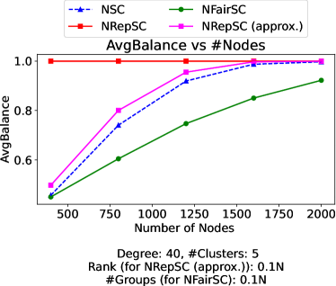
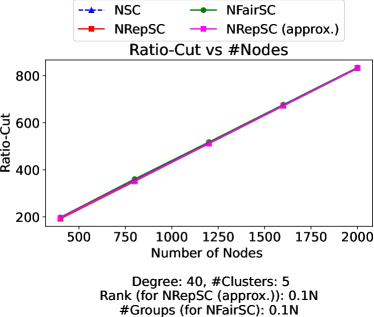
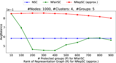
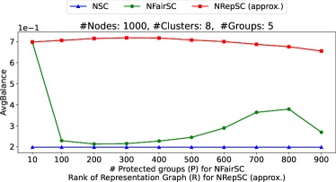
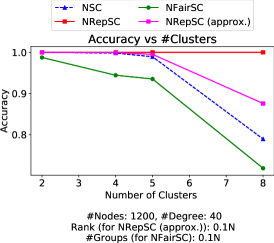
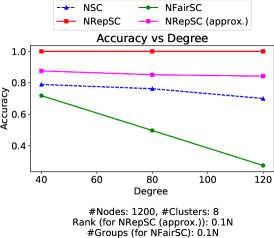
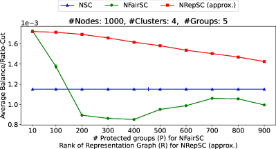
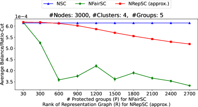
Figure 5 compares the performance of NRepSC with NFairSC [Kleindessner et al., 2019] and normalized spectral clustering (NSC) on synthetic $d$-regular representation graphs sampled from $\mathcal{R}$-PP, as described in Section 5. Figure 6 has the same semantics as Figure 5, but uses representation graphs sampled from the traditional planted partition model, as is the case with the second type of experiments in Section 5. Finally, Figure 7 uses the same FAO trade network as Section 5. All the results follow the same trends as URepSC in Section 5.

(a)

(b)

(c)

Figure 5: Comparing NRepSC with other “normalized” algorithms using synthetically generated $d$-regular representation graphs.

(a)

(b)

(c)

(d)

Figure 6: Comparing NRepSC (approx.) with NFairSC using synthetically generated representation graphs sampled from an SBM.

(a)

(b)

(c)

(d)

Figure 7: Comparing NRepSC (approx.) with NFairSC on FAO trade network.

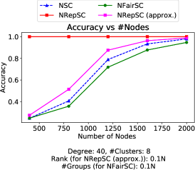
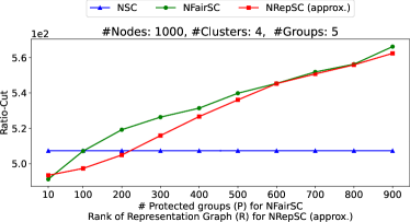
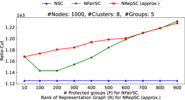
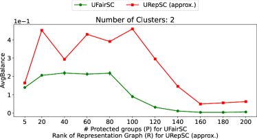
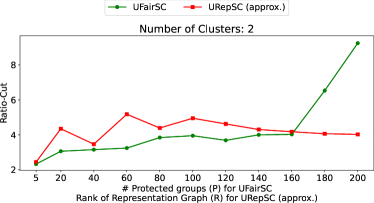
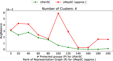
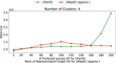
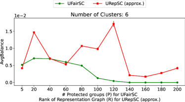
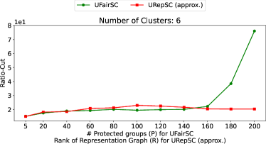
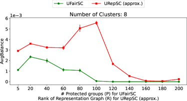
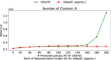
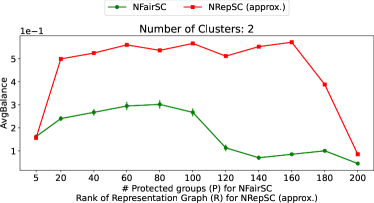
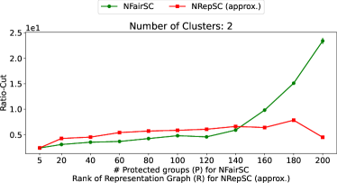
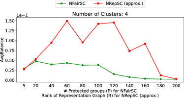
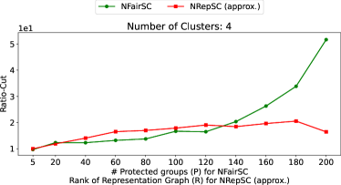
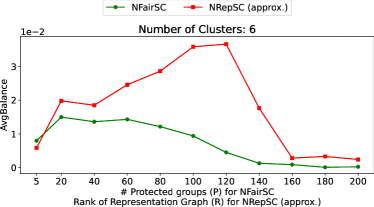
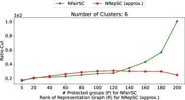
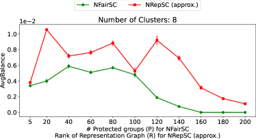
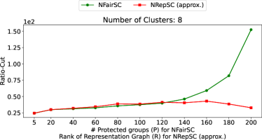
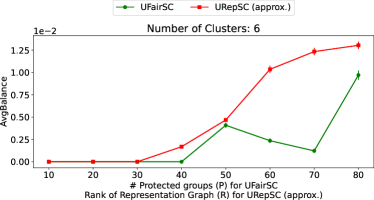
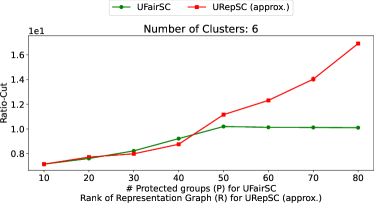
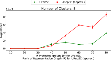
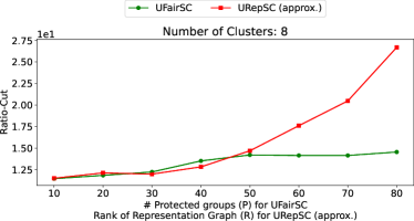
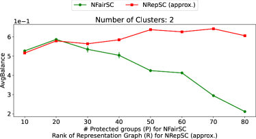
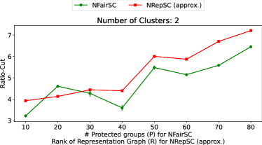
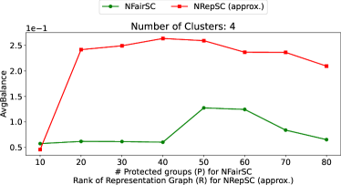
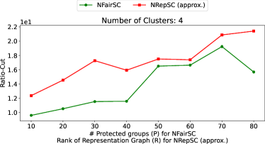
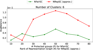
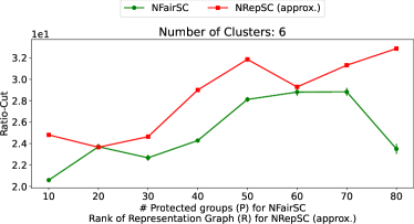
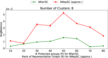
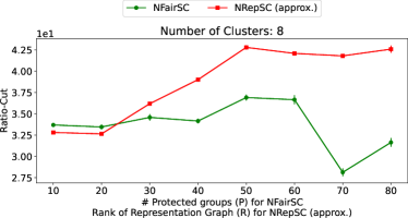
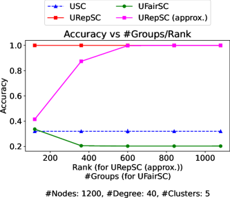
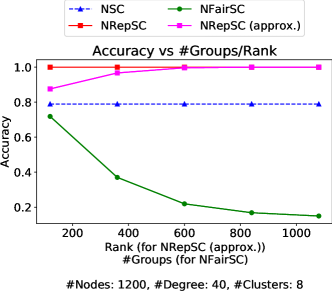
One may be tempted to think that UFairSC and NFairSC may perform well with a more carefully chosen value of $P$, the number of protected groups. However, Figures 8a and 8b show that this is not true. These figures plot the performance of UFairSC and NFairSC as a function of the number of protected groups $P$. Also shown is the performance of the approximate variants of our algorithms for various values of rank $R$. As expected, the accuracy increases with $R$ as the approximation of $\mathbf{R}$ becomes better but no similar gains are observed for UFairSC and NFairSC for various values of $P$.

(a)

(b)

Figure 8: Accuracy vs the values of $P$ and $R$ used by U/NFairSC and U/NRepSC, respectively, for $d$-regular representation graphs.

F.2 Experiments with the Air-Transportation Network

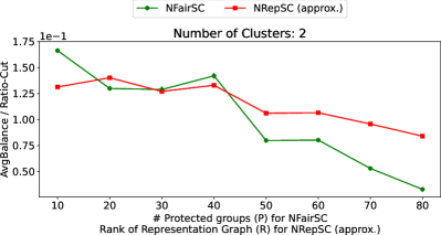
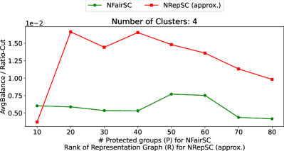
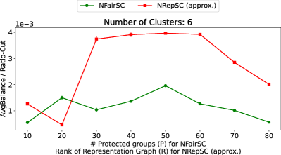
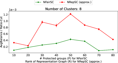
This section demonstrates the performance of URepSC (approx.) and NRepSC (approx.) on another real-world network called the Air-Transportation Network [Cardillo et al., 2013]. In this network, nodes correspond to airports, edges correspond to direct connections, and layers correspond to airlines. We took three designated “major” airlines (Air-France, British, and Lufthansa) and constructed a similarity graph by taking the union of the edges in these layers. Similarly, we constructed the representation graph by considering three “lowcost” airlines (Air-Berlin, EasyJet, and RyanAir). Nodes that were isolated in either of the similarity/representation graphs were dropped. The resulting graphs have $106$ nodes.

Figures 9 and 10 compare the performance of URepSC (approx.) and NRepSC (approx.) on this network with that of UFairSC and NFairSC respectively. The semantics of these plots are identical to the corresponding plots for the FAO trade network (Figures 3 and 7). As before, the value of $R$ can be chosen to get a high balance at a competitive ratio-cut.

(a)

(b)

(c)

(d)

Figure 9: Comparing URepSC (approx.) with UFairSC on the air-transportation network.

(a)

(b)

(c)

(d)

Figure 10: Comparing NRepSC (approx.) with NFairSC on the air-transportation network.

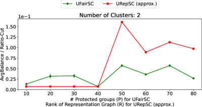
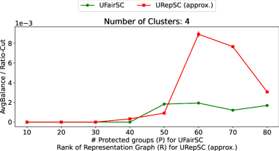
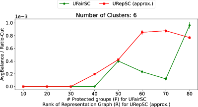
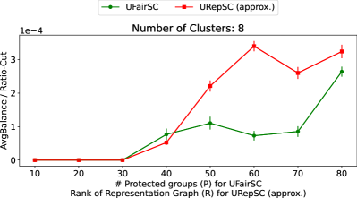
F.3 A few additional plots for URepSC

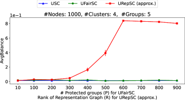
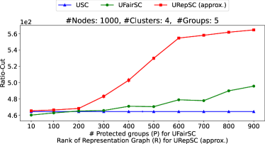
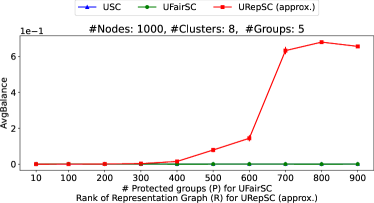
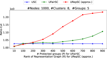
Figures 11 and 12 provide a few more configurations of $N$ and $K$ pairs for URepSC and have the same semantics as Figures 2 and 3 respectively.

(a)

(b)

(c)

(d)

Figure 11: Comparing URepSC (approx.) with UFairSC using synthetically generated representation graphs sampled from an SBM.

(a)

(b)

(c)

(d)

Figure 12: Comparing URepSC (approx.) with UFairSC on FAO trade network.

F.4 Numerical validation of time complexity

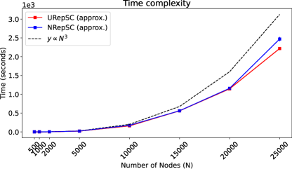
We close this section with a numerical validation of the time complexity of our algorithms. Recall from Remark 2 that URepSC has a time complexity of $O(N^{3})$. A similar analysis holds for NRepSC as well. URepSC (approx.) and NRepSC (approx.) involve an additional low-rank approximation step, but still have $O(N^{3})$ time complexity. Figure 13 plots the time in seconds taken by URepSC (approx.) and NRepSC (approx.) as a function of the number of nodes in the graph. We used representation graphs sampled from a planted partition model for these experiments with $K=4$, $R=0.5N$, and the remaining configurations same as in Section 5. The dotted line indicates the $O(N^{3})$ growth.

Figure 13: Time taken by U/NRepSC (approx.) as a function of the number of nodes in the graph.

Appendix G Plots with ratio-cut and average balance separated out

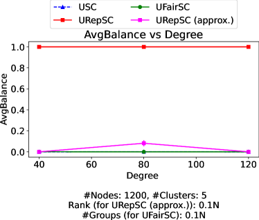
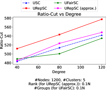
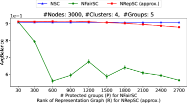
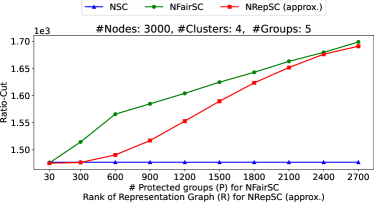
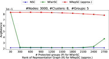
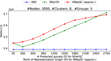
Up to this point, the plots either show accuracy (for $d$-regular graphs) or the ratio between average balance and ratio-cut (for planted partition based representation graphs and real-world networks) on $y$-axis as these quantities adequately convey the idea that our algorithms produce high-quality fair clusters. We now show the corresponding plots for each case with average balance and ratio-cut separated out.

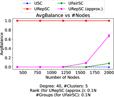
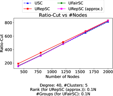
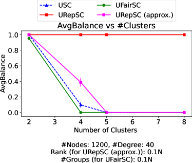
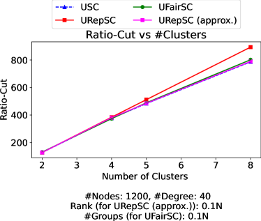
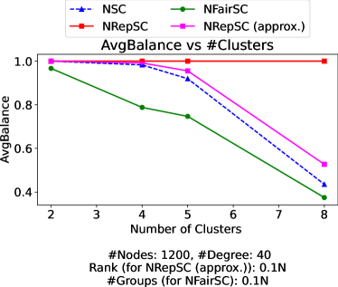
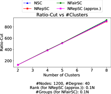
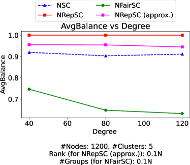
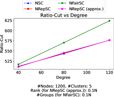
Figure 14 corresponds to Figure 1, Figure 15 to Figure 5, Figure 16 to Figure 11, Figure 17 to Figure 6, Figure 18 to Figure 12, Figure 19 to Figure 7, Figure 20 to Figure 9, and Figure 21 to Figure 10. As expected, individual fairness, which is a stricter requirement than group fairness, often comes at a higher cost in terms of ratio-cut. However, the difference in ratio-cut is competitive in most cases with a much higher gain in terms of average balance. As before, when the approximate variants of our algorithms are used, one can choose the rank $R$ used for approximation in a way that trades-off appropriately between a quality metric like the ratio-cut and a fairness metric like the average balance.

(a)

(b)

(c)

(d)

(e)

(f)

Figure 14: Comparing URepSC with other “unnormalized” algorithms using synthetically generated $d$-regular representation graphs.

(a)

(b)

(c)

(d)

(e)

(f)

Figure 15: Comparing NRepSC with other “normalized” algorithms using synthetically generated $d$-regular representation graphs.

(a)

(b)

(c)

(d)

(e)

(f)

(g)

(h)

Figure 16: Comparing URepSC with other “unnormalized” algorithms using representation graphs sampled from a planted partition model.

(a)

(b)

(c)

(d)

(e)

(f)

(g)

(h)

Figure 17: Comparing NRepSC with other “normalized” algorithms using representation graphs sampled from a planted partition model.

(a)

(b)

(c)

(d)

(e)

(f)

(g)

(h)

Figure 18: Comparing URepSC with other “unnormalized” algorithms on the FAO trade network.

(a)

(b)

(c)

(d)

(e)

(f)

(g)

(h)

Figure 19: Comparing NRepSC with other “normalized” algorithms on the FAO trade network.

(a)

(b)

(c)

(d)

(e)

(f)

(g)

(h)

Figure 20: Comparing URepSC with other “unnormalized” algorithms on the air transportation network.

(a)

(b)

(c)

(d)

(e)

(f)

(g)

(h)

Figure 21: Comparing NRepSC with other “normalized” algorithms on the air transportation network.

References

- Abbe [2018] Emmanuel Abbe. Community detection and stochastic block models: Recent developments. Journal of Machine Learning Research, 18(177):1–86, 2018.
- Ahmadian et al. [2017] Sara Ahmadian, Ashkan Norouzi-Fard, Ola Svensson, and Justin Ward. Better guarantees for k-means and euclidean k-median by primal-dual algorithms. Symposium on Foundations of Computer Science, 2017.
- Ahmadian et al. [2019] Sara Ahmadian, Alessandro Epasto, Ravi Kumar, and Mohammad Mahdian. Clustering without over-representation. In Proceedings of the 25th ACM SIGKDD International Conference on Knowledge Discovery & Data Mining, pages 267–275, 2019.
- Anderson et al. [2020] Nihesh Anderson, Suman K. Bera, Syamantak Das, and Yang Liu. Distributional individual fairness in clustering. arXiv, 2006.12589, 2020.
- Arthur and Vassilvitskii [2007] David Arthur and Sergei Vassilvitskii. k-means++: The advantages of careful seeding. Symposium on Discrete Algorithms, 2007.
- Banerjee and Ghosh [2006] Arindam Banerjee and Joydeep Ghosh. Scalable clustering algorithms with balancing constraints. Data Mining and Knowledge Discovery, 13:365–395, 2006.
- Bera et al. [2019] Suman Bera, Deeparnab Chakrabarty, Nicolas Flores, and Maryam Negahbani. Fair algorithms for clustering. Advances in Neural Information Processing Systems, 32:4954–4965, 2019.
- Bercea et al. [2019] Ioana O. Bercea, Martin Gross, Samir Khuller, Aounon Kumar, Clemens Rösner, Daniel R. Schmidt, and Melanie Schmidt. On the cost of essentially fair clusterings. APPROX-RANDOM, pages 18:1–18:22, 2019.
- Binkiewicz et al. [2017] Norbert Binkiewicz, Joshua T. Vogelstein, and Karl Rohe. Covariate assisted spectral clustering. Biometrika, 104(2):361–377, 2017.
- Cardillo et al. [2013] Alessio Cardillo, Jesús Gómez-Gardenes, Massimiliano Zanin, Miguel Romance, David Papo, Francisco del Pozo, and Stefano Boccaletti. Emergence of network features from multiplexity. Scientific Reports, 3(1344), 2013.
- Caton and Haas [2020] Simon Caton and Christian Haas. Fairness in machine learning: A survey. arXiv, 2010.04053, 2020.
- Chakrabarty and Negahbani [2021] Deeparnab Chakrabarty and Maryam Negahbani. Better algorithms for individually fair k-clustering. Advances in Neural Information Processing Systems, 34, 2021.
- Chen et al. [2019] Xingyu Chen, Brandon Fain, Liang Lyu, and Kamesh Munagala. Proportionally fair clustering. In Proceedings of the 36th International Conference on Machine Learning, 97:1032–1041, 2019.
- Chierichetti et al. [2017] Flavio Chierichetti, Ravi Kumar, Silvio Lattanzi, and Sergei Vassilvitskii. Fair clustering through fairlets. Advances in Neural Information Processing Systems, 30:5029–5037, 2017.
- Cucuringu et al. [2016] Mihai Cucuringu, Ioannis Koutis, Sanjay Chawla, Gary Miller, and Richard Peng. Simple and scalable constrained clustering: A generalized spectral method. Proceedings of the 19th International Conference on Artificial Intelligence and Statistics, 41:445–454, 2016.
- Davidson and Ravi [2005] Ian Davidson and S. S. Ravi. Clustering with constraints: Feasibility issues and the k-means algorithm. In Proceedings of the 5th SIAM Data Mining Conference, pages 138–149, 2005.
- Domenico et al. [2015] Manlio De Domenico, Vincenzo Nicosia, Alexandre Arenas, and Vito Latora. Structural reducibility of multilayer networks. Nature Communications, 6(1), 2015.
- Dwork et al. [2012] Cynthia Dwork, Moritz Hardt, Toniann Pitassi, Omer Reingold, and Richard Zemel. Fairness through awareness. ITCS ’12, pages 214––226, 2012.
- Esmaeili et al. [2020] Seyed Esmaeili, Brian Brubach, Aravind Srinivasan, and John Dickerson. Probabilistic fair clustering. Advances in Neural Information Processing Systems, 33, 2020.
- Esmaeili et al. [2021] Seyed Esmaeili, Brian Brubach, Aravind Srinivasan, and John Dickerson. Fair clustering under a bounded cost. Advances in Neural Information Processing Systems, 34, 2021.
- Fisman and Luca [2016] Ray Fisman and Michael Luca. Fixing discrimination in online marketplaces. Harvard Business Review, December 2016, 2016.
- Gao et al. [2017] Chao Gao, Zongming Ma, Anderson Y. Zhang, and Harrison H. Zhou. Achieving optimal misclassification proportion in stochastic block models. Journal of Machine Learning Research, 18:1–45, 2017.
- Ghoshdastidar and Dukkipati [2017a] Debarghya Ghoshdastidar and Ambedkar Dukkipati. Consistency of spectral hypergraph partitioning under planted partition model. Annals of Statistics, 45(1):289–315, 2017a.
- Ghoshdastidar and Dukkipati [2017b] Debarghya Ghoshdastidar and Ambedkar Dukkipati. Uniform hypergraph partitioning: Provable tensor methods and sampling techniques. Journal of Machine Learning Research, 18(1):1638–1678, 2017b.
- Harb and Shan [2020] Elfarouk Harb and Lam Ho Shan. Kfc: A scalable approximation algorithm for k-center fair clustering. Advances in Neural Information Processing Systems, 33, 2020.
- Holland et al. [1983] Paul W. Holland, Kathryn Blackmond Laskey, and Samuel Leinhardt. Stochastic blockmodels: First steps. Social Networks, 5(2):109–137, 1983.
- Kamvar et al. [2003] Sepandar D. Kamvar, Dan Klein, and Christopher D. Manning. Spectral learning. In Proceedings of the 18th International Joint Conference on Artificial Intelligence, pages 561–566, 2003.
- Kleindessner et al. [2019] Matthäus Kleindessner, Samira Samadi, Pranjal Awasthi, and Jamie Morgenstern. Guarantees for spectral clustering with fairness constraints. In Proceedings of the 36th International Conference on Machine Learning, 97:3458–3467, 2019.
- Kumar et al. [2004] Amit Kumar, Yogish Sabharwal, and Sandeep Sen. A simple linear time (1 + )-approximation algorithm for k-means clustering in any dimensions. Symposium on Foundations of Computer Science, 2004.
- Lei and Rinaldo [2015] Jing Lei and Alessandro Rinaldo. Consistency of spectral clustering in stochastic block models. The Annals of Statistics, 43(1):215–237, 2015.
- Lei and Zhu [2017] Jing Lei and Lingxue Zhu. A generic sample splitting approach for refined community recovery in stochastic block models. Statistica Sinica, 27(4):1639–1659, 2017.
- Li et al. [2009] Zhenguo Li, Jianzhuang Liu, and Xiaoou Tang. Constrained clustering via spectral regularization. In Proceedings of the IEEE Conference on Computer Vision and Pattern Recognition, pages 421–428, 2009.
- Lloyd [1982] Stuart P. Lloyd. Least squares quantisation in pcm. IEEE Transactions on Information Theory, 28(2):129–137, 1982.
- Lütkepohl [1996] Helmut Lütkepohl. Handbook of matrices. Wiley, 1996.
- Mahabadi and Vakilian [2020] Sepideh Mahabadi and Ali Vakilian. Individual fairness for k-clustering. In Proceedings of the 37th International Conference on Machine Learning, 119:6586–6596, 2020.
- Ng et al. [2001] Andrew Ng, Michael Jordan, and Yair Weiss. On spectral clustering: Analysis and an algorithm. Advances in Neural Information Processing Systems, 14, 2001.
- Rohe et al. [2011] Karl Rohe, Sourav Chatterjee, and Bin Yu. Spectral clustering and the high-dimensional stochastic blockmodel. The Annals of Statistics, 39(4):1878–1915, 2011.
- Rösner and Schmidt [2018] Clemens Rösner and Melanie Schmidt. Privacy preserving clustering with constraints. ICALP, 2018.
- Schmidt et al. [2018] Melanie Schmidt, Chris Schwiegelshohn, and Christian Sohler. Fair coresets and streaming algorithms for fair k-means clustering. arXiv, 1812.10854, 2018.
- Tremblay et al. [2016] Nicolas Tremblay, Gilles Puy, Remi Gribonval, and Pierre Vandergheynst. Compressive spectral clustering. In Proceedings of The 33rd International Conference on Machine Learning, 48:1002–1011, 2016.
- von Luxburg [2007] Ulrike von Luxburg. A tutorial on spectral clustering. Statistics and Computing, 17(4):395–416, 2007.
- von Luxburg et al. [2008] Ulrike von Luxburg, Mikhail Belkin, and Olivier Bousquet. Consistency of spectral clustering. The Annals of Statistics, 36(2):555–586, 2008.
- Vu [2018] Van Vu. A simple svd algorithm for finding hidden partitions. Combinatorics, Probability and Computing, 27(1):124–140, 2018.
- Vu and Lei [2013] Vincent Q. Vu and Jing Lei. Minimax sparse principal subspace estimation in high dimensions. The Annals of Statistics, 41(6):2905–2947, 2013.
- Wagner and Wagner [1993] Dorothea Wagner and Frank Wagner. Between min cut and graph bisection. Mathematical Foundations of Computer Science, 711:744–750, 1993.
- Wang and Davidson [2010] Xiang Wang and Ian Davidson. Flexible constrained spectral clustering. In Proceedings of the 16th ACM SIGKDD International Conference on Knowledge Discovery and Data Mining, pages 563–572, 2010.
- Wang et al. [2014] Xiang Wang, Buyue Qian, and Ian Davidson. On constrained spectral clustering and its applications. Data Mining and Knowledge Discovery, 28:1–30, 2014.
- Xu et al. [2009] Linli Xu, Wenye Li, and Dale Schuurmans. Fast normalized cut with linear constraints. IEEE Conference on Computer Vision and Pattern Recognition, 2009.
- Yu and Shi [2001] Stella X. Yu and Jianbo Shi. Grouping with bias. Advances in Neural Information Processing Systems, 14:1327–1334, 2001.
- Yu and Shi [2004] Stella X. Yu and Jianbo Shi. Segmentation given partial grouping constraints. IEEE Transactions on Pattern Analysis and Machine Intelligence, 26(2):173–183, 2004.
- Zhang et al. [2014] Yuan Zhang, Elizaveta Levina, and Ji Zhu. Detecting overlapping communities in networks using spectral methods. SIAM Journal on Mathematics of Data Science, 2(2):265–283, 2014.