Skin3D: Detection and Longitudinal Tracking
of Pigmented Skin Lesions in 3D Total-Body Textured Meshes

Abstract

We present an automated approach to detect and longitudinally track skin lesions on 3D total-body skin surface scans. The acquired 3D mesh of the subject is unwrapped to a 2D texture image, where a trained objected detection model, Faster R-CNN, localizes the lesions within the 2D domain. These detected skin lesions are mapped back to the 3D surface of the subject and, for subjects imaged multiple times, we construct a graph-based matching procedure to longitudinally track lesions that considers the anatomical correspondences among pairs of meshes and the geodesic proximity of corresponding lesions and the inter-lesion geodesic distances.

We evaluated the proposed approach using 3DBodyTex, a publicly available dataset composed of 3D scans imaging the coloured skin (textured meshes) of 200 human subjects. We manually annotated locations that appeared to the human eye to contain a pigmented skin lesion as well as tracked a subset of lesions occurring on the same subject imaged in different poses. Our results, when compared to three human annotators, suggest that the trained Faster R-CNN detects lesions at a similar performance level as the human annotators. Our lesion tracking algorithm achieves an average matching accuracy of 88% on a set of detected corresponding pairs of prominent lesions of subjects imaged in different poses, and an average longitudinal accuracy of 71% when encompassing additional errors due to lesion detection. As there currently is no other large-scale publicly available dataset of 3D total-body skin lesions, we publicly release over 25,000 3DBodyTex manual annotations, which we hope will further research on total-body skin lesion analysis.

I Introduction

Skin diseases are the most common reasons for patients to visit general practitioners in studied populations [schofield2011skin]. In the United States, melanoma-related cancer is estimated to increase by 100 thousand cases and cause more than 7000 deaths in 2021  [cancerfact2021], while the accessibility and wait time to see a dermatologist has become a concern [feng2018comparison, creadore2021insurance]. Leveraging the ability of artificial intelligence, especially in assisting the diagnosis of whole-body melanoma-related skin cancer, may improve the early diagnosis efficiency and improve patients’ outcomes [shellenberger2016melanoma].

When diagnosing a lesion, considering a large region of the skin and changes to lesions over time may provide additional helpful context not available when only considering a localized lesion at a single point in time. For example, visualizing a wide region of the skin may allow for multiple nevi to be detected, which is an important risk factor for melanoma [Gandini2005]. When monitoring a lesion over time, a nevi that is changing is an additional melanoma risk factor [Abbasi2004]. As an estimated 30% of melanomas evolve from existing nevi [Pampena2017], imaging and tracking a lesion across time may lead to a better understanding of how a lesion may transform and allow for early prediction of melanoma [Sondermann2019], reduce the number of excisions [tschandl2018sequential], and improve the prognosis of certain melanoma risk groups [haenssle2010selection]. Further, clinical studies suggest a benefit to patient outcome through longitudinal total-body skin imaging. Monitoring high risk patients with follow-up visits using total-body photography has been found to be associated with a greater rate of detecting lower-risk melanomas and overall survival [Strunck2020]. Combining digital total-body photography and dermoscopy to monitor patients over time has been found to enable early detection of melanoma with a low excision rate [Salerni2012].

While total-body skin imaging and longitudinal monitoring of skin lesions shows promise to improve melanoma detection, the amount of manual intervention required by human dermatologists to monitor and track changes of multiple lesions over the entire body is significant. With interest in collecting 3D reconstructions of the human body surface growing among dermatologists [Rayner2018, Primiero2019], we expect computer-aided approaches capable of detecting and tracking lesions over the entire body to reduce manual efforts and, in addition, serve as a system to flag high risk lesions for review by human dermatologists.

I-A Tracking and Detecting Multiple Lesions

The majority of computer-aided approaches to analyze pigmented skin lesions rely on static 2D colour images showing a single lesion, with limited works focusing on total-body photography or tracking lesions across time [Celebi2019, Pathan2018]. Rather than focusing on a single lesion, a wide-area (e.g., torso) region of the body can be imaged, where multiple lesions are visible. Using wide-area images, Lee2005 proposed an unsupervised approach to segment and count moles from 2D colour images of the back torso, but did not explore tracking lesions across time or incorporate total-body images.

Other computer-aided approaches explore changes to a single lesion across time. For example, to measure changes within a lesion across time, Navarro2019 proposed to register two dermoscopy images of the same lesion taken at different times and combined an automatic lesion segmentation approach to evaluate how a skin lesion evolves. Their approach assumes the corresponding lesions are known and the images are acquired using dermoscopy, which provide a more controlled field-of-view and scale than non-dermoscopy images.

Combining both wide-area images and lesions imaged over time, McGregor1998 registered (non-dermoscopy) photographs of human subjects by automatically detecting and selecting a matching subset of the lesions used to transform the images. Their study restricted the imaging to the torso regions and did not explore total-body imaging. Mirzaalian2016 proposed an approach to track skin lesions by detecting lesions on 2D wide-area skin images of the back of a body and matching lesions across images of the same subject using detected anatomical landmarks. li2016skin proposed a data augmentation strategy to synthesize large body images by blending skin lesion images onto images of back, legs, and chest using Poisson image editing, and then trained a fully convolutional neural network to perform lesion detection and a CNN to track lesions over time by estimating pixel-wise correspondence between a pair of images of the same body part. More recently, Soenksen2021 proposed a multi-stage workflow for detecting pigmented skin lesions from 2D wide-field images by first using a blob detection algorithm to extract all regions of interest in an image followed by CNN-based classification of these regions as suspicious or non-suspicious skin lesions or other classes (skin only, skin edge, or other background material).

Expanding the imaging field-of-view, total-body photography allows for the entire skin (or nearly the entire skin) to be imaged. Korotkov2015 developed an image acquisition system for photogrammetry-based total-body scanning of the skin to automatically acquire overlapping images of the patient’s skin. As the scanning system is in a carefully controlled environment, lesions can be automatically tracked across scans. Korotkov2019 further extended their system to improve mole matching among images, but did not explore 3D reconstruction of skin surfaces.

The 2014 work by Bogo2014a is similar to ours, where Bogo2014a performed whole-body 3D imaging, registered body scans acquired at multiple times, detected candidate lesions using linear discriminant analysis, and tracked lesions based on the registered body locations. We differ in our approach in that we use recently developed deep-learning based approaches to both detect lesions and register meshes, where our lesion detection step does not require choosing a threshold to isolate the skin nor post-processing as done in Bogo2014a. For lesion tracking, Bogo2014a used a common UV template to map anatomically corresponding locations to common texture elements within a texture image, while we perform our tracking on the 3D coordinates and consider geodesic distances between pairs of lesions. Finally, we note we use a larger dataset (200 vs. 22 unique subjects) with manually detected lesions (vs. artificially drawn lesions).

I-B Longitudinal Skin Datasets with Multiple Lesions

When compared to the large body of literature using static, single lesion images to analyze skin lesions, there are relatively few skin works for tracking multiple lesions across time. This is likely due to the lack of large standardized annotated datasets of longitudinal images available for computer-aided research, prompting a call by clinicians to gather longitudinal skin lesion images to train both clinicians and computer algorithms [Sondermann2019].

The publicly available FAUST dataset [Bogo2014] provides 300 3D body meshes, but lacks colour information about the surface of the body (e.g., skin colour information). Saint2018 created the 3DBodyTex dataset, which consists of 400 high resolution, 3D texture scans of 100 male and 100 female subjects captured in two different poses. Some lesions are visible on the skin; however, there are no lesion annotations publicly available. To the best of our knowledge, there currently is no large scale longitudinal dataset imaging a wide region of the skin with multiple annotated lesions publicly available. This lack of annotated skin lesion data makes it challenging to train machine learning models that require large amounts of labeled data and to benchmark competing approaches.

I-C Contributions

Methodologically, we propose a novel approach to detect and track skin lesions across 3D total-body textured meshes, where the colours on the surface of the subject are unwrapped to yield a 2D texture image, a Faster R-CNN model detects the lesions on the 2D texture images, and the detected lesions in 2D are mapped back to 3D coordinates. The detected lesions are tracked in 3D across pairs of meshes of the same subject using an optimization method that relies on deep learning-based anatomical correspondences and the geodesic distances between lesions. Our proposed approach has the potential for clinical utility in which a trained model detects the lesions on the 2D texture image, tracks the lesions across meshes in 3D, and displays the tracked lesions on the 3D mesh (or a 2D view of the 3D mesh) for the dermatologist to review, thereby reducing the initial manual effort required to densely annotate and track lesions over large skin regions. To the best of our knowledge, this is the largest evaluation of 3D total-body skin lesion detection and tracking on 3D textured meshes with skin colour information. Further, we make publicly available over 25,000 manual lesion annotations for 3DBodyTex.

II Methods

To detect lesions on the surface of 3D models and track lesions across time, we propose using 3D textured meshes, where the colours on the surface of the subject are mapped to 2D texture images, lesions are detected on 2D texture images, and tracked in 3D for longitudinal monitoring. A summary of the mathematical notation used in this paper is provided in Table II.

A scanned 3D object (e.g., human subject) is represented as a 3D mesh $\lx@glossaries@gls@link{notation}{mesh}{\leavevmode\mathcal{M}}=(\lx@glossaries@gls@link{notation}{vertices}{\leavevmode V},\lx@glossaries@gls@link{notation}{faces}{\leavevmode F},\lx@glossaries@gls@link{notation}{uvcoords}{\leavevmode U},\lx@glossaries@gls@link{notation}{textureImage}{\leavevmode I})$, with $N$ vertices $\lx@glossaries@gls@link{notation}{vertices}{\leavevmode V}\in\lx@glossaries@gls@link{notation}{realNumbers}{\leavevmode\mathbb{R}}^{N\times 3}$ where a single vertex $\lx@glossaries@gls@link{notation}{vertex}{\leavevmode v}\in\lx@glossaries@gls@link{notation}{vertices}{\leavevmode V}$ describes a 3D spatial coordinate; $\lx@glossaries@gls@link{notation}{face}{\leavevmode\xi}\in\lx@glossaries@gls@link{notation}{faces}{\leavevmode F}$ is the 3D face set which encodes the edges among the vertices; and $\lx@glossaries@gls@link{notation}{uvcoords}{\leavevmode U}\in\lx@glossaries@gls@link{notation}{realNumbers}{\leavevmode\mathbb{R}}^{N\times 2}$ are 2D UV texture coordinates that map vertices V to the texture image $\lx@glossaries@gls@link{notation}{textureImage}{\leavevmode I}\in\lx@glossaries@gls@link{notation}{realNumbers}{\leavevmode\mathbb{R}}^{W\times H\times 3}$, where $W$ and $H$ indicate the width and height of the colour texture image. Given meshes of the same subject scanned at $T$ different points in time $\{\lx@glossaries@gls@link{notation}{mesh}{\leavevmode\mathcal{M}}_{t}\}_{t=1}^{T}$, our goal is to detect the skin lesions within each scan, and match the corresponding lesions across the scans.

TABLE I: Summary of Notations

Glossary

$\xi$

A single 3D face

$F$

A set of 3D faces

$y$

2D lesion bounding box

$Y$

Set of 2D lesion bounding boxes

$\mathcal{M}$

A 3D mesh

$\theta$

The learned parameters of a Faster R-CNN

$\hat{y}$

Predicted 2D lesion bounding box

$\hat{z}$

Predicted 3D lesion center coordinates

$\hat{Y}$

Set of predicted 2D bounding boxes

$\hat{Z}$

Set of predicted 3D lesion center coordinates

$\phi$

Faster R-CNN

$\mathbb{R}$

The set of real numbers

$r$

A single 3D reconstructed vertex

$R$

The set of 3D reconstructed vertices

$A$

The vertices of the template mesh

$I$

A 2D texture image

$u$

A single UV texture coordinates

$U$

A set of UV texture coordinates

$v$

A single 3D vertex

$V$

A set of 3D vertices

II-A Detecting Lesions on 2D Texture Images

To detect lesions, we rely on the 2D texture image $I$, and represent a single lesion with a bounding box $\lx@glossaries@gls@link{notation}{lesion2d}{\leavevmode y}\in\lx@glossaries@gls@link{notation}{realNumbers}{\leavevmode\mathbb{R}}^{4}$ defined by 2D coordinates of two of its corners (2D coordinates of the top-left and bottom-right corners). We represent the bounding boxes of $M$ lesions within $I$ as $\lx@glossaries@gls@link{notation}{lesions2d}{\leavevmode Y}\in\lx@glossaries@gls@link{notation}{realNumbers}{\leavevmode\mathbb{R}}^{M\times 4}$.

We represent a lesion with a 2D bounding box since our goal in this work is to detect (i.e., localize and classify the existence of) the lesion from the background skin, which can be obtained via a bounding box, rather than acquiring a precise lesion segmentation. Precisely annotating the boundaries of the lesion is challenging due to the resolution of the texture images. Further, manually annotating 2D bounding boxes is far less time consuming for human annotators compared to 3D delineations.

Using the 2D texture image $I$ and corresponding lesion 2D bounding box annotations $Y$, we trained a region convolutional neural network (Faster R-CNN) (details in Section LABEL:skin3d:sec:rcnn) to predict 2D bounding box coordinates,

$$\lx@glossaries@gls@link{notation}{predLesions2d}{\leavevmode\hat{Y}}=\lx@glossaries@gls@link{notation}{rcnn}{\leavevmode\phi}\left(\lx@glossaries@gls@link{notation}{textureImage}{\leavevmode I};\lx@glossaries@gls@link{notation}{parameters}{\leavevmode\theta}\right)$$ (1)

where $\lx@glossaries@gls@link{notation}{rcnn}{\leavevmode\phi}(\cdot)$ is the Faster R-CNN trained to detect skin lesions with learned parameters $\theta$; and $\hat{Y}$ are the predicted 2D lesion bounding box coordinates within $I$. We use these 2D predicted bounding box lesion coordinates to measure the lesion detection performance between human and machine annotations (see results in Section LABEL:skin3d:sec:3dbodytex-static). However, for visualization purposes, and for tracking lesions across time, we require the 2D lesion locations to be mapped back to 3D coordinates.

Figure 1: A texture image with lesions detected manually (green box) and automatically (red box). The yellow borders indicate overlapping manual and automatic boxes. The blue box shows a closeup region of the texture image.

II-B Mapping the Detected 2D Lesions onto a 3D Mesh

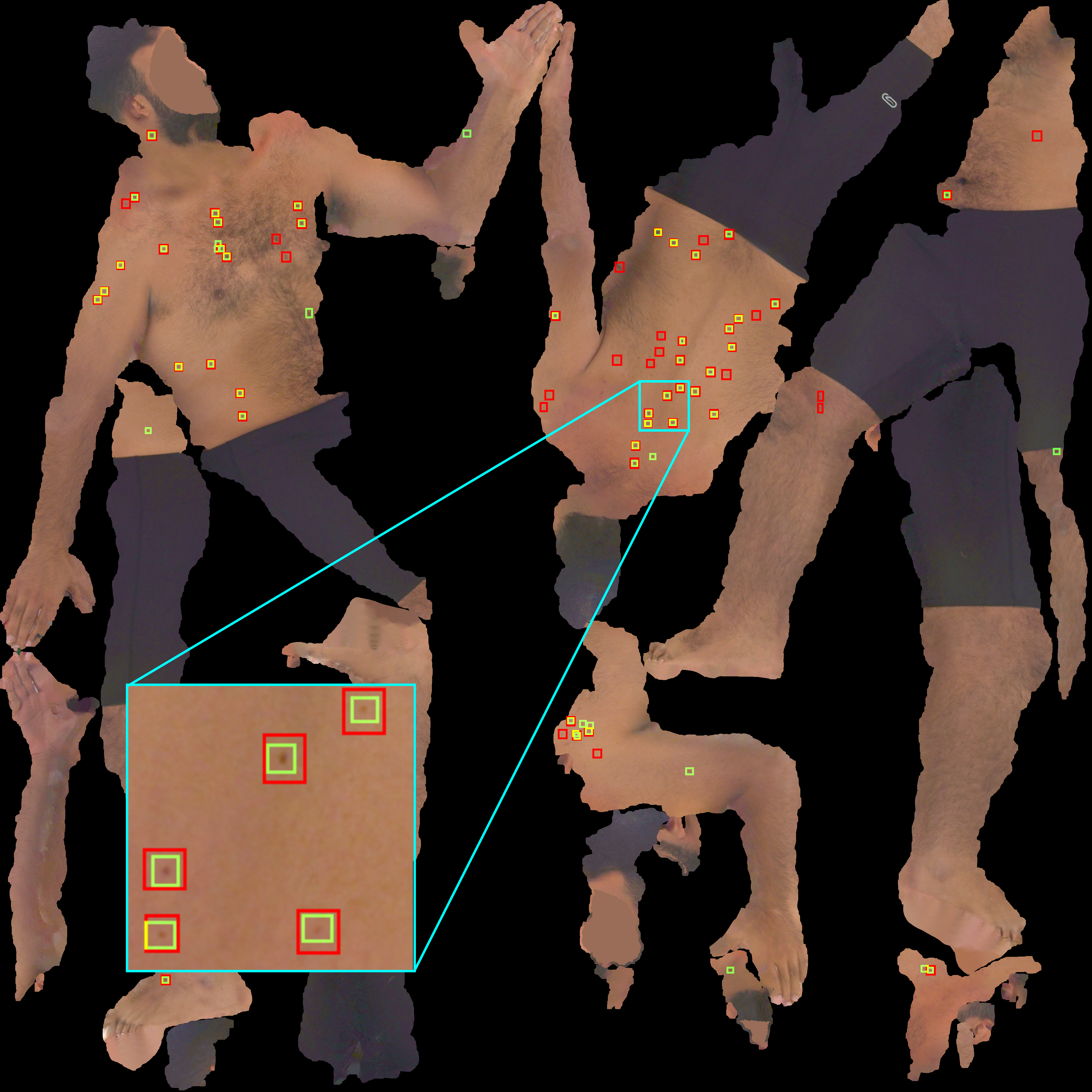
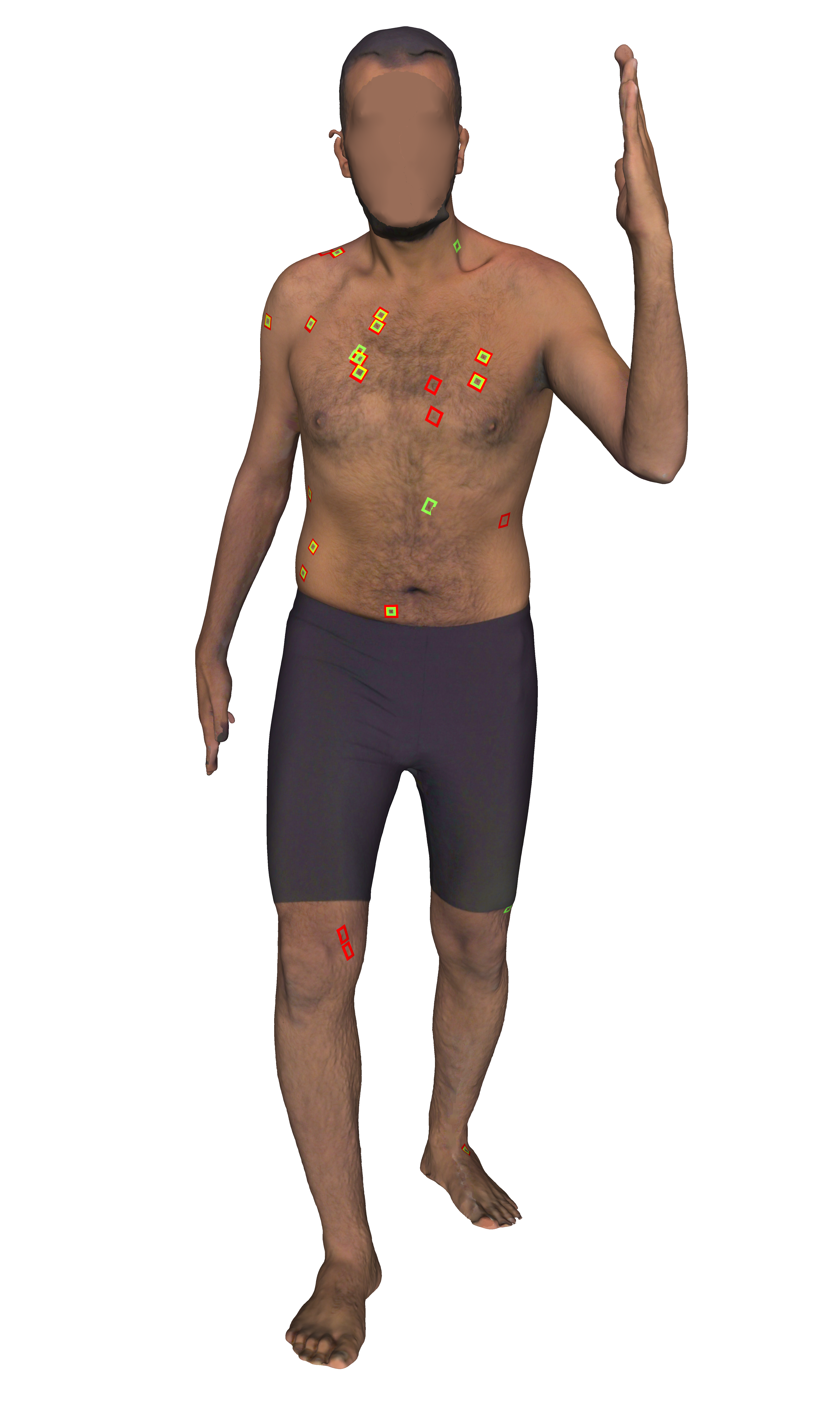
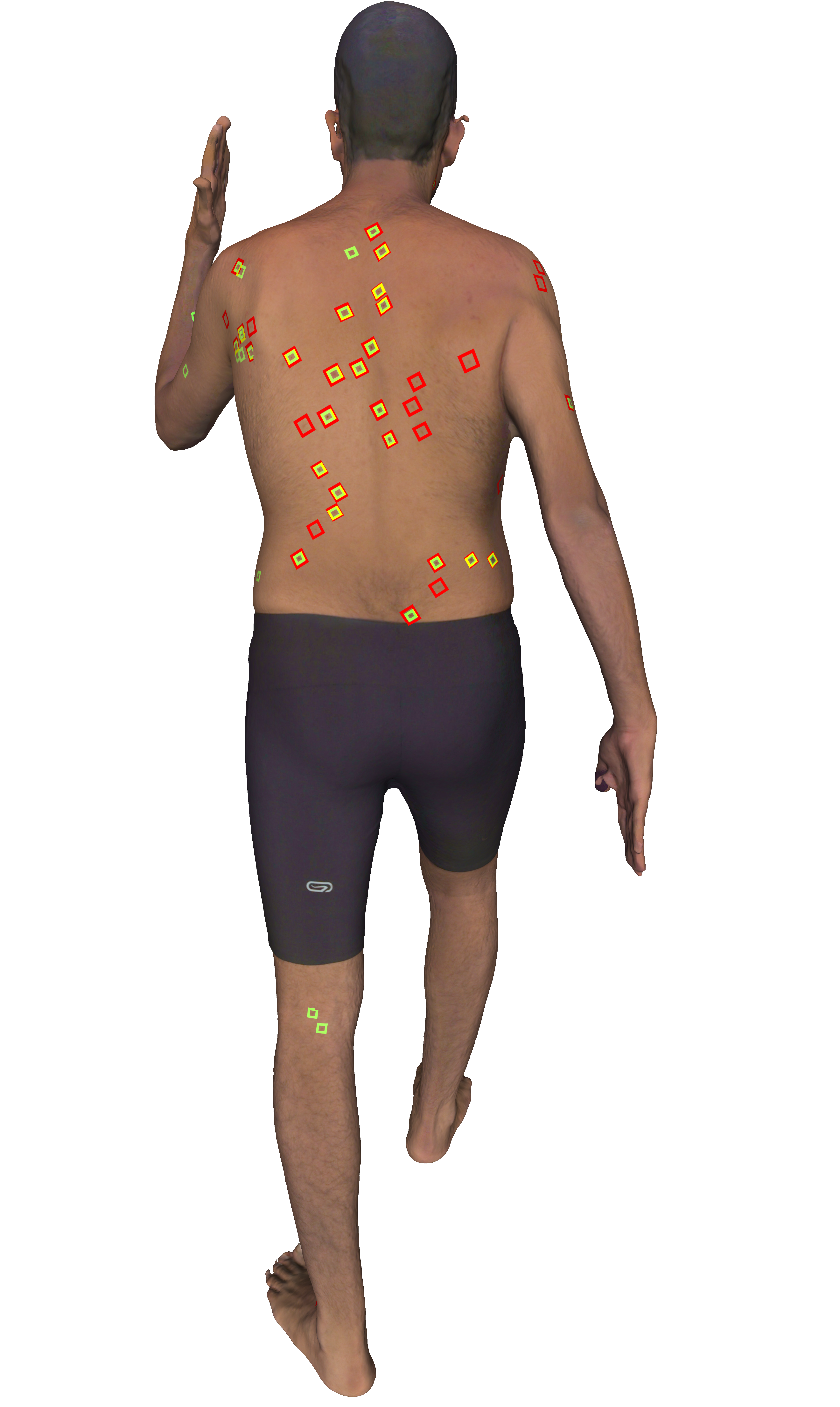
To visualize the 2D bounding boxes on the 3D mesh, we modify the texture elements based on the coordinates of the lesion bounding boxes $\hat{Y}$ in order to embed the bounding boxes within the original texture image $I$. The resulting lesion embedded texture image $I$ ${}_{\lx@glossaries@gls@link{notation}{predLesions2d}{\leavevmode\hat{Y}}}$ (Fig. 1) replaces the original texture image $I$ to show (Fig. 2) the embedded lesion annotations and texture information on the 3D mesh $\lx@glossaries@gls@link{notation}{mesh}{\leavevmode\mathcal{M}}_{\lx@glossaries@gls@link{notation}{predLesions2d}{\leavevmode\hat{Y}}}=(\lx@glossaries@gls@link{notation}{vertices}{\leavevmode V},F,\lx@glossaries@gls@link{notation}{uvcoords}{\leavevmode U},\lx@glossaries@gls@link{notation}{textureImage}{\leavevmode I}_{\lx@glossaries@gls@link{notation}{predLesions2d}{\leavevmode\hat{Y}}})$.

While bounding boxes are well suited for visualizing the localized lesions, we perform 3D analysis using the 3D positions of the lesions in order to better determine lesion correspondence across meshes, where the geodesic distances between lesions is computed on the 3D shape of the human body (discussed in Section II-C). We represent a lesion with the 3D vertex closest to the UV coordinates of the lesion’s 2D center point. Specifically, given the $i$-th lesion $\hat{y}$ ${}^{(i)}$ detected within $I$, we find the index of the UV coordinates closest to the center point of the 2D bounding box,

$$j^{*}=\operatorname*{argmin}_{j\in\{1,\dots,N\}}L_{1}(\lx@glossaries@gls@link{notation}{uvcoord}{\leavevmode u}^{(j)},f(\lx@glossaries@gls@link{notation}{predLesion2d}{\leavevmode\hat{y}}^{(i)}))$$ (2)

where $f(\cdot)$ computes the 2D center of the lesion bounding box and converts these image coordinates to the UV domain; $\lx@glossaries@gls@link{notation}{uvcoord}{\leavevmode u}^{(j)}\in U$ returns the $j$-th UV coordinates; and $L_{1}(\cdot)$ computes the $L_{1}$ distance between the mesh’s UV coordinates and the predicted lesion’s UV coordinates. As the indexes of the UV coordinates $U$ correspond to the indexes of the vertices $V$ (i.e., the UV coordinates that correspond to $v$ ${}^{(j)}$ are $\lx@glossaries@gls@link{notation}{uvcoord}{\leavevmode u}^{(j)}$), we obtain the mesh’s 3D vertex that corresponds to the 2D lesion coordinates by indexing the $j^{*}$-th vertex, $v$ ${}^{(j^{*})}$. Thus we map the $i$-th 2D lesion to the $j^{*}$-th 3D vertex within the mesh,

$$\lx@glossaries@gls@link{notation}{predLesion2d}{\leavevmode\hat{y}}^{(i)}\longrightarrow\lx@glossaries@gls@link{notation}{vertex}{\leavevmode v}^{(j^{*})}$$ (3)

where Eq. 2 is used to determine this mapping. We note that in Eq. 2 and Eq. 3 we approximate the location of the lesion with the nearest mesh vertex. We apply this approximation to reduce the complexity of computing the geodesic distances across meshes (discussed in section II-D).

Figure 2: The front and back of a subject with manual and automatically annotated lesions after mapping the texture image in Fig. 1 onto a 3D body mesh.

II-C Anatomically Corresponding Vertices Across Scans

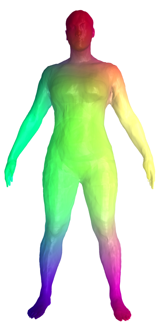
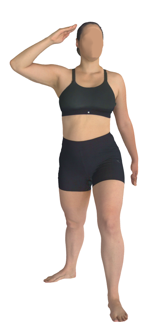
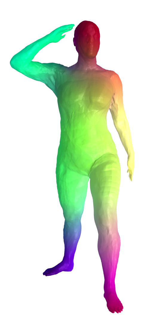
The same patient can be scanned at $T$ different times to form a set of 3D meshes $\{\lx@glossaries@gls@link{notation}{mesh}{\leavevmode\mathcal{M}}_{t}\}_{t=1}^{T}$. Our goal is to track the lesions across time, which requires us to account for variations in the subject across scans (e.g., pose may slightly vary across scans even if the subject is instructed to conform to a standard body position). As the 3D spatial coordinates alone are unsuitable to directly determine anatomical correspondence across meshes, we rely on 3D-CODED, a shape deformation network that uses deep learning to match deformable shapes [Groueix2018, Deprelle2019], to determine mesh correspondence. We use the human template, trained network, and default optimization parameters as provided by 3D-CODED, to determine anatomical correspondences of the vertices across scans of the same subject. The full details of the 3D-CODED approach are provided in Groueix2018, but here we highlight that 3D-CODED outputs reconstructed vertices $\lx@glossaries@gls@link{notation}{reconVertices}{\leavevmode R}\in\lx@glossaries@gls@link{notation}{realNumbers}{\leavevmode\mathbb{R}}^{N_{A}\times 3}$ that map to vertices in a common template $\lx@glossaries@gls@link{notation}{templateVertices}{\leavevmode A}\in\lx@glossaries@gls@link{notation}{realNumbers}{\leavevmode\mathbb{R}}^{N_{A}\times 3}$ (where $N_{A}$ are the number of vertices within the template), which we use to determine anatomical correspondences (Fig. 3). Specifically, given $\lx@glossaries@gls@link{notation}{reconVertices}{\leavevmode R}_{t}$ as the reconstructed vertices of $\lx@glossaries@gls@link{notation}{mesh}{\leavevmode\mathcal{M}}_{t}$, for the $i$-th vertex $\lx@glossaries@gls@link{notation}{vertex}{\leavevmode v}^{(i)}_{t}$ in $\mathcal{M}$ ${}_{t}$, we find the index $j^{*}$ of the closest reconstructed vertex,

$$j^{*}=\operatorname*{argmin}_{j\in\{1,\dots,N_{A}\}}L_{2}(\lx@glossaries@gls@link{notation}{reconVertex}{\leavevmode r}_{t}^{(j)},\lx@glossaries@gls@link{notation}{vertex}{\leavevmode v}^{(i)}_{t})$$ (4)

where $\lx@glossaries@gls@link{notation}{reconVertex}{\leavevmode r}_{t}^{(j)}\in\lx@glossaries@gls@link{notation}{reconVertices}{\leavevmode R}_{t}$ is the $j$-th reconstructed vertex; and $L_{2}(\cdot)$ computes the $L_{2}$ distance between the reconstructed and the original vertex. As the reconstructed vertices $\lx@glossaries@gls@link{notation}{reconVertices}{\leavevmode R}_{t}$ and $\lx@glossaries@gls@link{notation}{reconVertices}{\leavevmode R}_{t+1}$ share the common template $A$, the $j^{*}$-th vertex index gives us the anatomically corresponding vertex in $\lx@glossaries@gls@link{notation}{reconVertices}{\leavevmode R}_{t+1}$ (i.e., $\lx@glossaries@gls@link{notation}{reconVertex}{\leavevmode r}^{(j)}_{t}\in\lx@glossaries@gls@link{notation}{reconVertices}{\leavevmode R}_{t}$ and $\lx@glossaries@gls@link{notation}{reconVertex}{\leavevmode r}^{(j)}_{t+1}\in\lx@glossaries@gls@link{notation}{reconVertices}{\leavevmode R}_{t+1}$ can have different spatial coordinates, but point to the same anatomical location). Thus, we find the anatomically corresponding point in $\lx@glossaries@gls@link{notation}{mesh}{\leavevmode\mathcal{M}}_{t+1}$ by,

$$k^{*}=\operatorname*{argmin}_{k\in\{1,\dots,N_{t+1}\}}L_{2}(\lx@glossaries@gls@link{notation}{vertex}{\leavevmode v}_{t+1}^{(k)},r^{(j^{*})}_{t+1})$$ (5)

where $N_{t+1}$ is the number of vertices in $\mathcal{M}$ ${}_{t+1}$; the vertex $\lx@glossaries@gls@link{notation}{vertex}{\leavevmode v}^{(k)}_{t+1}\in\lx@glossaries@gls@link{notation}{mesh}{\leavevmode\mathcal{M}}_{t+1}$; and $\lx@glossaries@gls@link{notation}{reconVertex}{\leavevmode r}^{(j^{*})}_{t+1}\in\lx@glossaries@gls@link{notation}{reconVertices}{\leavevmode R}_{t+1}$ is the vertex reconstructed from $\lx@glossaries@gls@link{notation}{mesh}{\leavevmode\mathcal{M}}_{t+1}$ with the $j^{*}$-th index as determined by Eq. 4. With the $k^{*}$-th index, we then determine that $\lx@glossaries@gls@link{notation}{vertex}{\leavevmode v}^{(k^{*})}_{t+1}\in\lx@glossaries@gls@link{notation}{mesh}{\leavevmode\mathcal{M}}_{t+1}$ corresponds anatomically to $\lx@glossaries@gls@link{notation}{vertex}{\leavevmode v}^{(i)}_{t}\in\lx@glossaries@gls@link{notation}{mesh}{\leavevmode\mathcal{M}}_{t}$, which allows us to map anatomically corresponding vertices in $\lx@glossaries@gls@link{notation}{mesh}{\leavevmode\mathcal{M}}_{k}$ to vertices in $\lx@glossaries@gls@link{notation}{mesh}{\leavevmode\mathcal{M}}_{k+1}$.

(a) $\lx@glossaries@gls@link{notation}{mesh}{\leavevmode\mathcal{M}}_{t}$

(b) $R_{t}$

(c) $\lx@glossaries@gls@link{notation}{mesh}{\leavevmode\mathcal{M}}_{t+1}$

(d) $R_{t+1}$

Figure 3: Correspondence between two 3D meshes. (a) and (c) show meshes of the same subject in different poses. (b) and (d) show the reconstructed meshes, where the colours indicate vertex correspondence, obtained using 3D-CODED [Groueix2018].

II-D Tracking Lesions Across Poses and Time

Given a pair of meshes, $\lx@glossaries@gls@link{notation}{mesh}{\leavevmode\mathcal{M}}_{t}$ and $\lx@glossaries@gls@link{notation}{mesh}{\leavevmode\mathcal{M}}_{t+1}$, of the same subject imaged at different times, and the detected lesions, $\lx@glossaries@gls@link{notation}{predLesions2d}{\leavevmode\hat{Y}}_{t}$ and $\lx@glossaries@gls@link{notation}{predLesions2d}{\leavevmode\hat{Y}}_{t+1}$, detected on the 2D texture images (Eq. 1), our goal is to determine lesion correspondence. One approach, as proposed by Bogo2014a, is to register the meshes to a mesh template with a common UV mapping to form a standardized texture image with semantically aligned pixels, and compare the resulting pixel locations in the texture images to identify corresponding lesions. However, a drawback of this approach is that anatomically close 3D locations in the mesh may have large 2D distances in the texture image due to the UV mapping. This may be especially problematic in the cases when lesions occur near a seam (e.g., Fig. 1), where a small inaccuracy in the mesh registration process may place the lesions on the opposite side of the seam to be UV mapped to a far 2D location and create a large 2D distance. Thus, in this work, we perform our tracking based on 3D geodesic distances between vertices of registered meshes.

We map the center points of the 2D detected lesions to the closest vertices on the corresponding 3D meshes (Eq. 3). We denote these 3D vertices that correspond to lesion center points as $\lx@glossaries@gls@link{notation}{predLesions3d}{\leavevmode\hat{Z}}_{t}\in\lx@glossaries@gls@link{notation}{vertices}{\leavevmode V}_{t}$, where $\lx@glossaries@gls@link{notation}{predLesions3d}{\leavevmode\hat{Z}}_{t}$ is a subset of the vertices found within the original mesh’s vertices $\lx@glossaries@gls@link{notation}{vertices}{\leavevmode V}_{t}$ (i.e., $\lx@glossaries@gls@link{notation}{predLesion3d}{\leavevmode\hat{z}}^{(i)}_{t}\in\lx@glossaries@gls@link{notation}{predLesions3d}{\leavevmode\hat{Z}}_{t}$ is the 3D coordinates of the $i$-th lesion $\lx@glossaries@gls@link{notation}{predLesion2d}{\leavevmode\hat{y}}_{t}^{(i)}$ detected on the 2D texture image).

We seek to establish correspondence between the lesions $\text{<a href="\#glo.notation.predLesion3d"><span href="\#glo.notation.predLesion3d" title="Predicted 3D lesion center coordinates" class="ltx\_glossaryref ltx\_font\_italic"><span class="ltx\_text ltx\_glossary\_name"><xmath xmlns="http://dlmf.nist.gov/LaTeXML" id="S2.SS4.p3.1.m1.1.1d" xref="S2.SS4.p3.1.m1.1.1i.cmml"><xmapp id="S2.SS4.p3.1.m1.1.1e" xref="S2.SS4.p3.1.m1.1.1i.cmml"><xmtok name="hat" role="OVERACCENT" stretchy="false" id="S2.SS4.p3.1.m1.1.1f" xref="S2.SS4.p3.1.m1.1.1i.cmml">^</xmtok><xmarg id="S2.SS4.p3.1.m1.1.1g" xref="S2.SS4.p3.1.m1.1.1i.cmml"><xmtok role="UNKNOWN" font="italic" id="S2.SS4.p3.1.m1.1.1h" xref="S2.SS4.p3.1.m1.1.1i.cmml">z</xmtok></xmarg></xmapp></xmath></span></span></a>}$