Generation and Effects of Electromotive Force in Turbulent Stochastic Reconnection

Abstract

Reconnection is an important process that rules dissipation and diffusion of magnetic energy in plasmas. It is already clear that its rate is enhanced by turbulence, and that reconnection itself may increase its stochasticity, but the main mechanism that connects these two effects is still not completely understood. The aim of this work is to identify, from the terms of the electromotive force, the dominant physical process responsible for enhancing the reconnection rate in turbulent plasmas. We employ full three-dimensional numerical simulations of turbulence driven by stochastic reconnection and estimate the production and dissipation of turbulent energy and cross-helicity, the amount of produced residual helicity, and determine the relation between these quantities and the reconnection rate. We observe the development of the electromotive force in the studied models with plasma-$\beta=0.1-2$ and the Lundquist number $S=10^{-5}-10^{-4}$. The turbulent energy and residual helicity develop in the large-scale current sheet, with the latter decreasing the effects of turbulent magnetic diffusion. We demonstrate that the stochastic reconnection, apart from the turbulence, can produce a significant amount of cross-helicity as well. The cross-helicity to turbulent energy ratio, however, has no correlation with the reconnection rate. We show that its sufficiently large value is not a necessary condition for fast reconnection to occur. The results suggest that cross-helicity is inherent to turbulent fields, but the reconnection rate enhancement is possibly caused by the effects of magnetic turbulent diffusion and controlled by the residual helicity.

I Introduction

Magnetic reconnection is a fundamental process that controls magnetic energy removal and dissipation in astrophysical systems. It is crucial for heating, acceleration of particles, and mass accretion. At large scales the reconnection rate provided by the standard Sweet–Parker theory (Parker, 1957; Sweet, 1958) is negligible, as estimated by the relation $V_{\mathrm{rec,SP}}\approx V_{\mathrm{A}}S_{L}^{-1/2}\ll V_{\mathrm{A}}$, where $S_{L}=LV_{\mathrm{A}}/\eta$ is the Lundquist number, $L$ - a longitudinal scale of the reconnecting flux tube, $V_{A}$ - the Alfvén speed, and $\eta$ - magnetic resistivity. Given the high conductivity of plasmas and scales of astrophysical systems, one finds very low values of $V_{\mathrm{rec,SP}}$ even for astrophysical scenarios where reconnection is known to occur at fast rates (see, e.g., Zweibel and Yamada, 2009; Yamada, Kulsrud, and Ji, 2010; Gonzalez and Parker, 2016; Lazarian et al., 2020).

Conceptually, fast reconnection can only be achieved by a mechanism for which $V_{\mathrm{rec}}$ does not depend on $S_{L}$ or, if so, should depend on it weakly (e.g. logarithmically). The earliest numerical works on fast reconnection using particle-in-cell (PIC) simulations considered collisionless instabilities or the Hall effect in the generalized Ohm’s law (see, e.g., Shay and Drake, 1998; Shay et al., 1998; Birn et al., 2001; Cassak, Shay, and Drake, 2005). More recently, Liu et al. (2017) proposed a modified Sweet–Parker theory demonstrating, that by controlling the opening angle of the outflow region, the reconnection rate can be fast. They suggested that the mechanism responsible for the opening of the outflow region is tearing/plasmoid instability. The Sweet–Parker model outflow scale limitation imposed by microphysics has been challenged by Lazarian and Vishniac (1999), for which the outflow width scale is determined by the scales of turbulence rather than plasma microphysics. This fast reconnection model in the presence of turbulence was successfully tested in a number of numerical studies (e.g., Kowal et al., 2009, 2012; Higashimori, Yokoi, and Hoshino, 2013; Takamoto, Inoue, and Lazarian, 2015; Jabbari et al., 2016).

Due to the ubiquitous nature of turbulence in astrophysical sites, one may understand fast reconnection as a general process as well. Typically turbulence is understood as being driven externally, at large scales, such as found in quiescent giant molecular clouds (see Armstrong, Rickett, and Spangler, 1995; Padoan et al., 2009; Chepurnov and Lazarian, 2010; Falceta-Gonçalves et al., 2015), however, it may arise naturally, e.g., by collisionless kink instability (Markidis et al., 2014), the shock-induced reconnection (Bessho et al., 2020), the Kelvin-Helmholtz vortex-induced reconnection (Nakamura et al., 2020), or due to plasmoid and/or Kelvin-Helmholtz instabilities within the stochastic reconnection (Kowal et al., 2020).

The interlink between turbulence and fast reconnection is, however, still an open issue. It requires more studies to understand what makes turbulence an important mechanism for accelerating reconnection rates. As pointed by Lazarian and Vishniac (1999), one of the possible roles of turbulence would be the enlargement of the outflow scales of the reconnection region. From a different perspective, Yokoi and Hoshino (2011) proposed the cross-helicity, generated by the turbulent motions, as the key ingredient for fast reconnection, and that sites of non-vanishing cross-helicity should be those where this process occurs. Instead of the outflow scale, this model focuses on the enlargement of the regions of inter-crossing field lines. Yokoi, Higashimori, and Hoshino (2013) studied the space-temporal distribution of transport coefficients due to turbulence by means of the mean-field approach. In such idealized model, the reconnection properties were obtained from the balance between the transport enhancement due to the turbulent energy and its suppression due to the cross-helicity. According to Yokoi, Higashimori, and Hoshino (2013), a possible explanation would be that the increase of cross-helicity suppresses the growth of turbulent transport with consequent confinement of magnetic diffusion in smaller regions, and therefore increasing the magnetic reconnection rate. Under this model, a self-consistent determination of timescales has also been studied (Widmer, Büchner, and Yokoi, 2019). Indeed, the importance of cross-helicity for the turbulent diffusion of magnetic fields has been extensively studied, mostly focused on the evolution of the dynamo effect. Although cross-helicity is globally conserved in ideal incompressible fluids (Woltjer, 1958), this is not the case in turbulent compressible plasmas (e.g. Marsch and Mangeney, 1987; Sur and Brandenburg, 2009; Webb et al., 2014a, b).

Recent cross-helicity studies in the solar wind using Parker Solar Probe (PSP) measurements of the proton density and velocity, together with the measurements of magnetic field, have shown that the alignment between velocity and magnetic field at convective scales presents a large number of negative value events, which is due to the presence of magnetic switchbacks, or brief periods where the magnetic field polarity reverses (McManus et al., 2020). Their abundance and short timescales as seen by PSP in its first encounter is a new front of study, and their precise origin is still unknown. They argue that these must be local kinks in the magnetic field and not due to small regions of opposite polarity on the surface of the Sun, which could be possibly related to stochastic reconnection, i.e., the reconnection in the presence of weakly stochastic fluctuations of velocity or magnetic field (as in Lazarian and Vishniac, 1999).

The intrinsic relation between turbulence and fast reconnection has become clearer in the past few years by means of several theoretical and numerical studies (see, e.g., Eyink et al., 2013; Eyink, 2015; Jafari and Vishniac, 2019; Lazarian et al., 2020). Still, not all aspects of this close relation are understood thoroughly. Here, we have addressed one of the gaps by studying, from three-dimensional high resolution magnetohydrodynamic (MHD) numerical simulations of stochastic magnetic reconnection, the loci and effects of terms of electromotive force, the turbulent energy, and the cross-helicity for the reconnection rates. The scope of this work is to determine whether there is a correlation between the growth of reconnection rates and the local enhancement of turbulent energy, cross-helicity, or residual helicity.

The manuscript is organized as follows. The theoretical description of electromotive force is provided in Section II. In Sections III and IV we describe the numerical simulations used for this work and the procedure of the field separation into mean and fluctuating components in order to determine the studied quantities, respectively. These sections are followed by the description of the main results in Section V. Finally, in Section VI, we present our discussion and main conclusions.

II Electromotive force in the context of mean-field theory

The electromotive force in the mean-field dynamo has been studied analytically and numerically for a few decades already (see, e.g., Moffatt, 1978; Krause and Raedler, 1980; Yoshizawa, 1990; Brandenburg and Subramanian, 2005; Schrijver and Siscoe, 2009; Hughes and Tobias, 2010; Charbonneau, 2014; Brandenburg, 2018). The mean-field approach has been also applied to turbulent magnetic reconnection (Yokoi and Hoshino, 2011; Yokoi, Higashimori, and Hoshino, 2013; Higashimori, Yokoi, and Hoshino, 2013; Widmer, Büchner, and Yokoi, 2019). Here, we briefly describe parts relevant to this work following Yokoi, Higashimori, and Hoshino (2013), where the production, transport and diffusion of turbulent energy, cross-helicity, and residual helicity and their relation to the electromotive force has been investigated analytically in details.

We consider a system for which the evolution is governed by non-ideal compressible isothermal MHD equations:

$$\frac{\partial\rho}{\partial t}+\nabla\cdot\left(\rho\vec{u}\right)=0,$$ (1)

$$\begin{split}\frac{\partial\left(\rho\vec{u}\right)}{\partial t}+\nabla\cdot\left[\rho\vec{u}\vec{u}+(a^{2}\rho+\frac{B^{2}}{2\mu_{0}})I-\frac{\vec{B}\vec{B}}{\mu_{0}}\right]=\\ \nu\rho\left[\nabla^{2}\vec{u}+\frac{1}{3}\nabla\left(\nabla\cdot\vec{u}\right)\right],\end{split}$$ (2)

$$\frac{\partial\vec{B}}{\partial t}-\nabla\times\left(\vec{u}\times\vec{B}-\eta\vec{J}\right)=0,$$ (3)

where $\rho$, $\vec{u}$, and $\vec{B}$ are plasma density, velocity and magnetic field, respectively, $\vec{J}\equiv\nabla\times\vec{B}$ is the current density, $I$ is the identity matrix, and $a$, $\mu_{0}$, $\nu$, and $\eta$ describe the isothermal speed of sound, the magnetic permeability constant, the viscosity, and the magnetic resistivity, respectively. Using the Reynolds decomposition applied to all fields,

$$\rho\rightarrow\bar{\rho}+\rho^{\prime},\,\vec{u}\rightarrow\vec{U}+\vec{u}^{\prime},\vec{B}\rightarrow\vec{B}+\vec{b}^{\prime},$$ (4)

where $\bar{\rho}$, $\vec{U}$, $\vec{B}$ describe the mean density, velocity, and magnetic field, respectively, and $\rho^{\prime}$, $\vec{u}^{\prime}$, and $\vec{b}^{\prime}$ their corresponding fluctuating parts, one can separate the evolution of the mean and fluctuating fields. In the equations governing the evolution of mean fields, however, will appear terms resulting from the averaging of the high order products of fluctuating fields discussed in more details below. For convenience, Eqs. 1-3 and the equations describing the mean and fluctuating fields evolution can be expressed in dimensionless units once the density is given in the units of $\rho_{0}$, the velocity and magnetic field in the units of Alfvén speed, $V_{A}=B_{0}/\sqrt{\mu_{0}\rho_{0}}$, being $B_{0}$ the characteristic magnetic field strength. Under this normalization, time is expressed in the units of Alfvén time $t_{A}$.

The main quantities involved in the studies of effects of turbulence on mean fields are represented by the Reynolds stress tensor ${\cal R}=\langle\vec{u}^{\prime}\vec{u}^{\prime}-\vec{b}^{\prime}\vec{b}^{\prime}\rangle$ and the turbulent electromotive force $\vec{E}_{M}\equiv\langle\vec{u}^{\prime}\times\vec{b}^{\prime}\rangle$, where brackets $\langle\rangle$ indicate spatial averaging at a given scale defining the mean components. Using the fluctuating parts one can define the kinetic and magnetic turbulent energies, $K_{u^{\prime}}\equiv\frac{1}{2}\langle\vec{u}^{\prime 2}\rangle$ and $K_{b^{\prime}}\equiv\frac{1}{2}\langle\vec{b}^{\prime 2}\rangle$, respectively, cross-helicity $W\equiv\langle\vec{u}^{\prime}\cdot\vec{b}^{\prime}\rangle$, and residual helicity $H\equiv\langle-\vec{u}^{\prime}\cdot\vec{\omega}^{\prime}+\vec{b}^{\prime}\cdot\vec{j}^{\prime}\rangle$, where $\vec{\omega}^{\prime}=\nabla\times\vec{u}^{\prime}$ and $\vec{j}^{\prime}=\nabla\times\vec{b}^{\prime}$.

According to Yokoi, Higashimori, and Hoshino (2013) model the productions of turbulent energy $P_{K}$ and cross-helicity $P_{W}$ are described by two terms, one involving the electromotive force $\vec{E}_{M}$ and another involving the Reynolds stress ${\cal R}^{ij}$, being explicitly

$$P_{K}=-\vec{E}_{M}\cdot\vec{J}-{\cal R}^{ab}\frac{\partial U^{a}}{\partial x^{b}},$$ (5)

and

$$P_{W}=-\vec{E}_{M}\cdot\vec{\Omega}-{\cal R}^{ab}\frac{\partial B^{a}}{\partial x^{b}},$$ (6)

where $\vec{J}=\nabla\times\vec{B}$ and $\vec{\Omega}=\nabla\times\vec{U}$ are the mean current density and vorticity, respectively (see Eqs. 29a and 30a in Yokoi, Higashimori, and Hoshino, 2013). The turbulent energy and cross-helicity are subject to dissipation due to the presence of explicit viscosity and resistivity (Eqs. 29b and 30b in Yokoi, Higashimori, and Hoshino, 2013), described by

$$\varepsilon_{K}=\nu\bigg{\langle}\frac{\partial u^{\prime a}}{\partial x^{b}}\frac{\partial u^{\prime a}}{\partial x^{b}}\bigg{\rangle}+\eta\bigg{\langle}\frac{\partial b^{\prime a}}{\partial x^{b}}\frac{\partial b^{\prime a}}{\partial x^{b}}\bigg{\rangle}$$ (7)

and

$$\varepsilon_{W}=\left(\nu+\eta\right)\bigg{\langle}\frac{\partial u^{\prime a}}{\partial x^{b}}\frac{\partial b^{\prime a}}{\partial x^{b}}\bigg{\rangle}.$$ (8)

It should be noted, that cross-helicity $W$, and its production $P_{W}$ and dissipation $\varepsilon_{W}$ are not sign-definite.

The electromotive force $\vec{E}_{M}$ is important. It describes the effects of turbulence on the mean field induction equation

$$\frac{\partial\vec{B}}{\partial t}=\nabla\times\left(\vec{U}\times\vec{B}-\eta\vec{J}+\vec{E}_{M}\right).$$ (9)

In order to close the system of equations for the large-scale fields, it is necessary to express the electromotive force in terms of large-scale $\vec{B}$ and $\vec{U}$, and their derivatives (see, e.g., Moffatt, 1978; Yoshizawa, 1990; Schrijver and Siscoe, 2009; Hughes and Tobias, 2010; Yokoi, Higashimori, and Hoshino, 2013). Under the assumption of inhomogeneous MHD turbulence (Yoshizawa, 1990; Yokoi, 2013; Yokoi, Higashimori, and Hoshino, 2013) the electromotive force can be expressed as

$$\vec{E}_{M}=\bar{\alpha}\vec{B}-\bar{\beta}\vec{J}+\bar{\gamma}\vec{\Omega},$$ (10)

where $\bar{\alpha}$, $\bar{\beta}$, and $\bar{\gamma}$ are transport coefficients determined by the statistical properties of turbulence

$$\bar{\alpha}=\tau_{\alpha}H,\,\bar{\beta}=\tau_{\beta}K,\,\bar{\gamma}=\tau_{\gamma}W,$$ (11)

where $\tau_{\alpha}$, $\tau_{\beta}$, and $\tau_{\gamma}$ are turbulent time scales of residual helicity $H$, turbulent energy $K=K_{u^{\prime}}+K_{b^{\prime}}$, and cross-helicity $W$, respectively. Inserting Eq. (10) into Eq. (9) gives

$$\frac{\partial\vec{B}}{\partial t}=\nabla\times\left[\vec{U}\times\vec{B}-\left(\eta+\bar{\beta}\right)\vec{J}\right]+\nabla\times\left(\bar{\alpha}\vec{B}+\bar{\gamma}\vec{\Omega}\right).$$ (12)

The last term represents the generation mechanism of the mean field $\vec{B}$, while $\bar{\beta}$ acts as the localized turbulent magnetic diffusivity effect.

The dynamical balance between the turbulent energy and cross-helicity is expected to result in fast reconnection (Yokoi and Hoshino, 2011; Yokoi, Higashimori, and Hoshino, 2013). Yokoi and Hoshino (2011) demonstrated analytically that the reconnection rate can be significantly enhanced if the ratio of the cross-helicity to the total turbulent energy $|W|/K$ is larger than a threshold of 0.1. Furthermore, Yokoi (2018a, b) considered the effects of compressibility on the electromotive force which additionally enhances the reconnection rate (see also Widmer, Büchner, and Yokoi, 2019). The mean-field model by Yokoi, Higashimori, and Hoshino (2013) has been confirmed to be valid by comparing it to high resolution simulations of plasmoid instability with a filtering procedure applied (Widmer, Büchner, and Yokoi, 2016a).

III Numerical modeling

The numerical experiments planned in this work were performed in order to identify the generation and evolution of the terms mentioned above in a reconnection generated current sheath. Differently to previous works though, we have studied the problem of electromotive force generation and evolution from the full numerical solution of the non-ideal, compressible, 3-dimensional MHD equations (Eqs. 1–3). The domain is defined as a 3D rectangular domain with physical dimensions $L\times 4L\times L$ (assuming $L=1$), the base resolution of $32\times 128\times 32$, and the local mesh refinement up to $5$ levels resulting in the effective resolution of $512\times 2048\times 512$ (the effective grid size being $h=1/512$ along all directions). The refinement criterion was based on the normalized value of vorticity and current density to follow the turbulence development. We set periodic boundaries along the X and Z directions, and non-reflecting open boundaries along the Y direction, at which we apply the condition of the derivative normal to the boundary plane equal to zero. By placing the Y boundaries far from the initial current sheet, we guarantee that the boundary conditions do not affect the development of turbulence, or the reconnection process itself.

As initial conditions, for the reconnection to be ignited, we consider a Harris current sheet configuration with a guide field, i.e. $\vec{B}=\left[\tanh\left(y/\delta\right),0,B_{g}\right]$, as in our previous works (Kowal et al., 2017, 2020). The density profile was set to $\rho(y)=1+\frac{1}{\beta\left(1+B_{g}^{2}\right)}\mathrm{sech}^{2}\left(y/\delta\right)$ to make the total pressure uniform initially. The isothermal speed of sound is given by $a=\sqrt{\frac{\beta}{2}\left(1+B_{g}^{2}\right)}$, where $\beta=p/p_{mag}$ is the plasma-$\beta$ parameter, and $p=a^{2}\rho$ and $p_{mag}=B^{2}/2$ are thermal and magnetic pressures, respectively. We used Prandtl number $Pr=\frac{\eta}{\nu}=1$ with viscosity and resistivity equal $\eta=\nu=S^{-1}$ (see Eqs. 2 and 3 for explicit viscous and resistive terms). The initial thickness of the current sheet was set to $\delta=3.16\times 10^{-3}$ and the uniform guide field to $B_{g}=0.1$. The velocity field was initiated with fluctuations represented by $100$ Fourier modes of random phases and directions, the amplitude of each mode equal to $10^{-3}$ and wavenumber $k\approx 64\pi$. The random velocity fluctuations were set in a narrow region within the vertical distance up to 0.09 from the initial current sheet. This was done by applying a window function to the perturbations generated from the Fourier modes, defined by a function along the $y$ coordinate only, $f(y)=\cos^{2}{\left(\frac{\pi}{2}\zeta\right)}$, where $\zeta=\mathrm{min}\left(1,\mathrm{max}\left(0,(y-0.05)/0.04\right)\right)$. The window function produces a step function with the transition of a given width smoothed by squared cosine. Therefore, the initial setup is controlled by the upstream plasma-$\beta$, the current sheet thickness $\delta$, the guide field strength $B_{g}$, and the Lundquist number $S$.

The MHD equations (1)–(3) were solved using a high-order shock-capturing adaptive refinement Godunov-type code AMUN (https://bitbucket.org/amunteam/amun-code) with 5^th-order Optimized Compact Monotonicity Preserving reconstruction of Riemann states (Ahn and Lee, 2020), the HLLD Riemann flux solver (Mignone, 2007), and the 3rd-order 4-step Strong Stability Preserving Runge-Kutta (SSPRK) method (Gottlieb, Ketcheson, and Shu, 2011) for time integration. Due to the initial upstream density and the strength of reconnecting component of magnetic field being unities they resulted in the velocity and simulation time units $[v]=V_{A}=1$ and $[t]=t_{A}=L/V_{A}=1$, respectively.

We present here results for three models with different values of plasma-$\beta$ and Lundquist number $S$: $\beta=0.1$ and $S=10^{5}$ (model A), $\beta=2$ and $S=10^{5}$ (model B) and $\beta=2$ and $S=10^{4}$ (model C) run for $10-30$ Alfvén times.

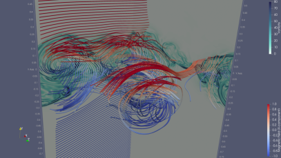
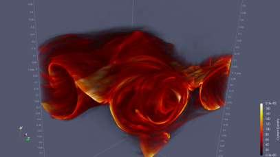
Figure 1: Visualization of the selected magnetic lines and vorticity projected on the computational domain boundaries (left plot) and the current density intensity (right plot) for model A at the final moment $t=10$. Only the region of the computational domain where the turbulence is developed is shown, from around -0.5 to 0.5 along the Y-direction. The full domain extends from -2 to 2 along this direction.

IV Field Separation Procedure

Once the numerical simulations are run, for the several data sets of different timescales, we want to determine the electromotive force, turbulent energy and cross-helicity terms. In order to do so, as explained in §II, we must decompose the mean and fluctuating terms of the variables evolved.

The separation which guarantees the self-consistent determination of both mean and fluctuating fields is the Reynolds decomposition. It satisfies a certain set of rules known as Reynolds rules, i.e. $\langle cf\rangle=c\langle f\rangle$, $\langle f+g\rangle=\langle f\rangle+\langle g\rangle$, $\langle f^{\prime}\rangle=0$, $\langle\langle f\rangle\rangle=\langle f\rangle$, $\langle\langle f\rangle\cdot g\rangle=\langle f\rangle\langle g\rangle$, $\langle f^{\prime}\cdot g^{\prime}\rangle=\langle f\cdot g\rangle-\langle f\rangle\cdot\langle g\rangle$, etc., where $\langle\rangle$ means the ensemble average, $f,g$ are arbitrary fields, $f^{\prime}=f-\langle f\rangle$, $g^{\prime}=g-\langle g\rangle$ are the fluctuating parts, and $c$ is a constant. The equations presented in §II were derived under the assumption of the Reynolds decomposition.

In this work, the mean fields were determined by spatial averaging over the $XZ$-planes. This type of averaging satisfies the Reynolds rules and is adequate to the symmetry of our problem, which is characterized by an initial sharp transition of the magnetic field across the $y=0$ plane and near uniformity far from the turbulent region during the whole evolution. Since our simulations are based on the adaptive mesh, before the averaging was applied, we used trilinear interpolation to represent the fields on the uniform mesh equivalent to the effective resolution. By subtracting the large-scale components from the original fields we obtained the fluctuating parts $\vec{u}^{\prime}(x,y,z)$ and $\vec{b}^{\prime}\left(x,y,z\right)$. The averages of products of fluctuating parts were determined using the corresponding rule listed in the previous paragraph. They determine the electromotive force $\vec{E}_{M}$ and other related quantities. The described procedure produces mean fields varying solely along the Y-direction. This results in the Y-components of the mean vorticity and current density to be zero. Additionally, in order to fulfill the divergence-free condition of the mean $\vec{B}$ we assumed its $Y$-component to be zero. It should be clarified, that the averaging procedure applied to the initial velocity fluctuations results in the mean vorticity $\vec{\Omega}$ which is not zero at $t=0$. $\vec{\Omega}$ reaches very small amplitudes, slightly above $5\times 10^{-3}$ near the initial current sheet in our setup.

The applied averaging procedure dictates the scope of our approach, which is to study the response of the global magnetic reconnection process, defined by the profiles along the $y$ coordinate, to the presence of longitudinal (with respect to the current sheet plane) turbulent fluctuations produced by the reconnection itself. Clearly, the short-wave fluctuations of the mean fields along the Y-direction are not perfectly averaged by this procedure, as explained above. Nevertheless, by using the periodicity along the X and Z directions, we guarantee that the variations of the mean fields along the Y-direction is the result of the initial velocity perturbation and developed turbulence.

We should remark that the averaging over the XZ-planes can affect the interpretation of our results in the context of Yokoi, Higashimori, and Hoshino (2013) model, which was derived under the assumption of inhomogeneous turbulence. Still, the analytical framework of their model was an inspiration for the studies presented in this manuscript. Our averaging procedure treats any kind of variability along the X or Z directions as the fluctuating part. We do not analyze the horizontal profiles of the quantities which are not sign-definite, such as cross-helicity. We plan to apply to our simulations alternate averaging procedures, such as Gaussian filtering (see, e.g., §2 in Sagaut, 2006), in the future.

V Results

In this work we study the evolution of electromotive force $\vec{E}_{M}$, the turbulent energy $K$, its production $P_{K}$ and dissipation $\varepsilon_{K}$, the cross-helicity $W$, its production $P_{W}$ and dissipation $\varepsilon_{W}$, the residual helicity $H$, the scalar product $\vec{J}\cdot\vec{B}$, and the ratio $|W|/K$, using the mean-field approach inspired by the model presented in Yokoi, Higashimori, and Hoshino (2013), in stochastic turbulent reconnection (see Kowal et al., 2017, 2020). Moreover, we investigate the causality between these quantities and the reconnection rate $V_{rec}$ measured in these models.

In Figure 1 we show an example visualization of the model A at the final time $t=10$. In the left plot, we show the selected magnetic lines with the red and blue colors identifying their orientation with respect to the X-axis (red for the parallel and blue indicating the anti parallel orientations with respect to the X axis). As seen by the degree of the line wandering, the magnetic field above and below the turbulent region is relatively laminar. The oppositely oriented field lines are mixed in the turbulent region resulting in a complex current density structure, seen in the right plot of Figure 1. Together with the magnetic lines we show two cuts of the vorticity distribution in the left plot, one along the XY and another along the YZ plane, which identify the turbulent region. Clearly, the developed turbulence directly affects the reconnection process, as well as, its rate.

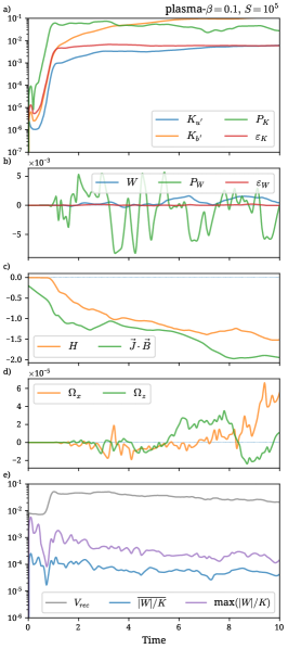
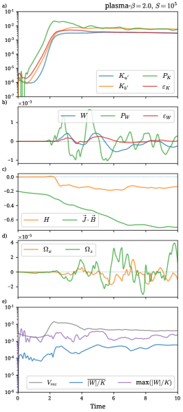
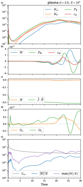
Figure 2: Evolution of (a) the kinetic $K_{u^{\prime}}$ and magnetic $K_{b^{\prime}}$ turbulent energies, the production $P_{K}$ and dissipation $\varepsilon_{K}$ of turbulent energy, (b) the cross-helicity $W$, its production $P_{W}$ and dissipation $\varepsilon_{W}$, (c) the residual helicity $H$ and the scalar product $\vec{J}\cdot\vec{B}$, (d) the large-scale vorticity components, $\Omega_{x}$ and $\Omega_{z}$, and (e) the mean ratio of cross-helicity to total turbulent energy $\overline{|W|/K}$ and the reconnection rate $V_{rec}$, for models A, B, and C (left, middle, and right, respectively). All quantities shown in plots a)-d) are integrated over the computational domain. The mean value of the ratio $|W|/K$ was calculated over a region near the mid-plane containing 99% of total turbulent energy (see Fig. 3).

In Figure 2 we present time evolution of turbulent energies $K_{u^{\prime}}$ and $K_{b^{\prime}}$, the turbulent energy production $P_{K}$ and dissipation $\varepsilon_{K}$ (a), the cross-helicity $W$, its production $P_{W}$ and dissipation $\varepsilon_{W}$ (b), the residual helicity $H$ and the scalar product $\vec{J}\cdot\vec{B}$ (c), the large-scale components of vorticity $\Omega_{x}$ and $\Omega_{z}$ (d), all integrated over the $y$ coordinate. In addition, in the last row (e) of Figure 2, we show the maximum value of the ratio of the absolute value of cross-helicity over total turbulent energy, $|W|/K$, as well as, the mean value averaged over the mid-plane region containing 99% of the total turbulent energy and the reconnection rate $V_{rec}$ determined using the method described in Kowal et al. (2009). The estimation of $V_{rec}$ is based on the conservation of the magnetic flux related to the reconnecting component $B_{x}$. It tracks the temporal variation of the absolute value of $B_{x}$ integrated over the computational domain taking into account the field brought to the system through the open Y-boundaries, $V_{rec}=\left[\iint_{A}{U_{y}|B_{x}|\,dxdz}-\frac{d}{dt}\iiint_{V}{|B_{x}|\,dxdydz}\right]/B_{0}$, where $A$ is the Y boundary area, $V$ is the computational domain volume, and $B_{0}$ is the amplitude of $B_{x}$ averaged over $A$. Since our Y-boundaries are far from the current sheet and the region of developed turbulence, the terms related to the shear and dissipation of magnetic field at the boundaries could be neglected (see §4 in Kowal et al., 2009, for more details).

In all models shown in Figure 2 the evolution can be divided into two stages: the growth and the saturation phases. Focusing on the growth phase first, we see that its duration depends both on plasma-$\beta$ and the Lundquist number $S$. Comparing the evolution of kinetic turbulent energy $K_{u^{\prime}}$, the estimated growth rates (within the period of exponential growth) are $\leavevmode\nobreak\ 12.4$, $\leavevmode\nobreak\ 6.2$, and $\leavevmode\nobreak\ 0.7$ for model A, B, and C, respectively, indicating that both lower plasma-$\beta$ and higher Lundquist number favor the quicker development of turbulence in stochastic reconnection. The magnetic turbulent energy is characterized by similar growth rates: $\leavevmode\nobreak\ 12.1$, $\leavevmode\nobreak\ 5.2$, and $\leavevmode\nobreak\ 0.7$, for model A, B, and C, respectively. This suggests a close interaction of velocity and magnetic eddies exchanging the turbulent energy between them. Apart from the increase of turbulent energies, we also observe a similar growth of the production and dissipation of turbulent energy (Fig. 2a, green and red lines, respectively).

It is interesting to see that, during the growth phase, there is essentially no generation of cross-helicity $W$ and the residual helicity $H$ (Fig. 2b, c). The production of cross-helicity $P_{W}$ and it dissipation $\varepsilon_{W}$ are relatively negligible during this stage too. This indicates that these quantities start to be generated once the full turbulent cascade is formed. As shown in (Kowal et al., 2017), the cascade is build up from the small scales toward the large scales during the growth phase (inverse cascade).

The only variable sensitive to the growth of the turbulent energies, except the turbulent energy, is the reconnection rate $V_{rec}$, however, only in the high Lundquist number models A and B. There, the growth of the reconnection rate is visible exactly during the growth phase observed in the turbulent energy evolution. In model C, even though the turbulent energy increases by over two orders of magnitude, $V_{rec}$ constantly decays.

The fact that the reconnection rate reaches larger values in the low plasma-$\beta$ model, and the turbulence develops faster in this regime, could be explained by higher degree of compressibility. Low plasma-$\beta$ means that plasma motions can be mildly or even weakly supersonic in the vicinity of the current sheet, increasing the compression of plasma, which in turn reduces the importance of magnetic tension. This results in easier mixing of the magnetic flux within the turbulent region, and more efficient turbulent dissipation ($\bar{\beta}$-effect). If the explicit diffusion (viscosity and resistivity) is sufficiently large, however, it dissipates the fluctuations at scales comparable to the current sheet thickness on time scales shorter than the reconnection time scale, and cannot sufficiently affect the reconnection rate. However, the fluctuations at scales $l>\delta$ can affect the shape of the current sheet, which ejects the kinetic energy from the reconnection outflow regions.

Analyzing the evolution of turbulent energies, $K_{u^{\prime}}$ and $K_{b^{\prime}}$ (blue and orange, respectively) during the saturation phase in Figure 2a, we see that in the case of high Lundquist number models A and B (left and middle), the kinetic turbulent energy $K_{u^{\prime}}$ reaches values about $5.9\times 10^{-3}$ and $3.2\times 10^{-3}$, respectively, while in the case of model C (right) this energy is over an order of magnitude smaller, slightly above $10^{-4}$ at the end of the simulation. The final turbulent magnetic energy $K_{b^{\prime}}$ level strongly depends on the values of plasma-$\beta$ and $S$, reaching over $10^{-1}$, $\sim 6\times 10^{-3}$, and $\sim 1.5\times 10^{-4}$ for models A, B, and C, respectively. In model A the turbulent magnetic energy is nearly an order of magnitude larger than the kinetic one, while in models with plasma-$\beta=2$ they are nearly in equipartition with $K_{u^{\prime}}$ slightly smaller than $K_{b^{\prime}}$. In the lower Lundquist number model C the kinetic and magnetic energies reach the maximum level of over $10^{-4}$ around time $t=15$, however, they start to slowly decrease afterwords. The production and dissipation of turbulent energy are shown in Figure 2a with green and red lines, respectively. $P_{K}$ saturates at levels around $4\times 10^{-2}$ and $5.6\times 10^{-3}$, a difference of around 7 times, for models A and B, respectively. It is interesting that the dissipation $\varepsilon_{K}$ for these models reaches somewhat less discrepant levels, of around $6\times 10^{-3}$ and $3\times 10^{-3}$, respectively. Significantly different levels of $P_{K}$ and $\varepsilon_{K}$ suggest continuous production of turbulent energy, as can be seen clearly in the case of low plasma-$\beta$ model A, where the levels of $K_{u^{\prime}}$ and $K_{b^{\prime}}$ increase gradually even after reaching the saturation. In model C, the production $P_{K}$ and dissipation $\varepsilon_{K}$ increase until time about $t=20$, with $P_{K}$ being larger than $\varepsilon_{K}$ by a factor of around 2. After $t=20$, $P_{K}$ and $\varepsilon_{K}$ start to decay with the dissipation slightly overcoming the production. In all these cases, the positive balance of $P_{K}$ over $\varepsilon_{K}$ indicates the growth of turbulent energy. Normally, the turbulent energy or cross-helicity could be produced in one place and then transported through out the domain. Due to the fact that we assume large-scae $B_{y}=0$ to guarantee the divergence-free large-scale magnetic field, the large-scale transport, expressed by the $\vec{B}\cdot\nabla$ terms (Eqs. 29c and 30c in Yokoi, Higashimori, and Hoshino, 2013), is therefore null. This seems to be consistent with the visualizations presented in Figure 1, which demonstrate that indeed the turbulent region is constrained in the vertical direction. Therefore, the net production of the turbulent energy and cross-helicity are determined by $P_{K}-\varepsilon_{K}$ and $P_{W}-\varepsilon_{W}$, respectively.

In the second row of Figure 2 we show the evolution of the cross-helicity $W$ (blue), its production $P_{W}$ (green) and dissipation $\varepsilon_{W}$ (red) integrated over the computational domain. We see that $W$ oscillates around zero with an increasing amplitude reaching around $10^{-3}$ and $5\times 10^{-4}$ at later times for models A and B (left and middle panels), respectively. The mean values averaged over the last 4 time units for these models are $7\times 10^{-4}$ and $-2\times 10^{4}$, respectively. The periods of increasing and decreasing cross-helicity are well correlated with the sign of the production $P_{W}$ in all models. It is interesting to see that the dissipation of cross-helicity $\varepsilon_{W}$ is much weaker in models with $S=10^{5}$ indicating that the production $P_{W}$ is mainly responsible for the oscillating character of $W$. In the case of model C (right panel) the cross-helicity tends to negative values, significantly weaker in terms of amplitudes (by two orders of magnitude) when comparing to models A or B. The dissipation $\varepsilon_{W}$ is only weaker by a factor of around 2 comparing to the production in this case, in contrast to other models, most probably due to large values of viscosity and resistivity.

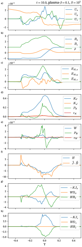
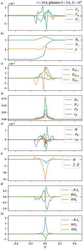
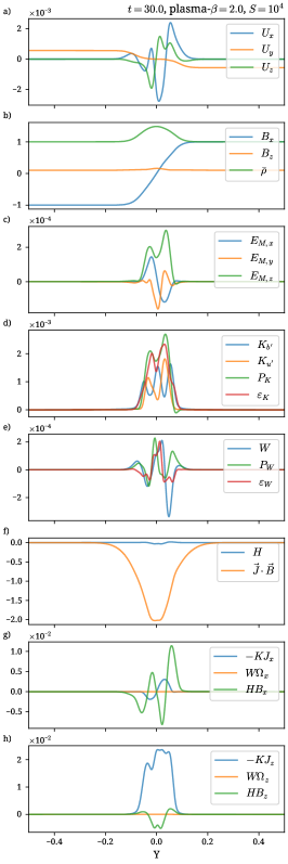
Figure 3: From top to bottom, profiles of (a) the mean velocity $\vec{U}$ components, (b) the mean magnetic field components ($B_{x}$ and $B_{z}$) and density $\bar{\rho}$, (c) the electromotive force $\vec{E}_{M}$ components, (d) the kinetic $K_{u^{\prime}}$ and magnetic $K_{b^{\prime}}$ turbulent energies, the production $P_{K}$ and dissipation $\varepsilon_{K}$ of turbulent energy, (e) the cross-helicity $W$ and its production $P_{W}$ and dissipation $\varepsilon_{W}$, (f) the residual helicity $H$ and the scalar product of the large-scale current density and magnetic field $\vec{J}\cdot\vec{B}$, (g) the comparison of terms $-KJ_{x}$, $W\Omega_{x}$, and $HB_{x}$, and (h) the comparison of terms $-KJ_{z}$, $W\Omega_{z}$, and $HB_{z}$, for models A, B, and C (left, middle, and right, respectively) at the final simulation times.

In the third row of Figure 2 we show the evolution of the mean residual helicity $H$. This quantity seems to be strongly related to plasma-$\beta$. It grows gradually to negative values reaching around $-1.5$ at the final time of simulation in the case of model A. For model B, after a very short period of small positive values at around $t=2$, it quickly decays to values below $-0.1$ and oscillates around $-0.15$. The model C manifests much weaker and more delayed development of $H$. After long initial oscillations around zero, with a very weak amplitude, it quickly decreases to $-8\times 10^{-3}$ only after $t=18$ and returns to zero at the later times. For comparison, we show in the same plot the evolution of the integrated quantity $\vec{J}\cdot\vec{B}$, which, according to Eq. 43 in Widmer, Büchner, and Yokoi (2016b), determines the evolution of $\bar{\alpha}$. The evolution of $\vec{J}\cdot\vec{B}$ resembles the evolution of $H$ only in the low plasma-$\beta$ model A. In model B, the scalar product of large-scale current density and magnetic field constantly decreases saturating only after about $t=7$ at the value around $-0.7$, much lower than $H$ which saturates much earlier. In the case of model C, however, $\vec{J}\cdot\vec{B}$ reaches values around $-0.3$ very quickly, as compared to nearly negligible values of $H$.

The next row in Figure 2 (row d) shows the evolution of the large-scale components of vorticity integrated over the domain. As noted earlier, the initial vorticity is weak but not zero. As seen in these plots, the large-scale vorticity fluctuates around zero with amplitude increasing during the whole evolution, with the Z component dominating over the X one. The increase of $\Omega_{z}$ is especially well seen in models B and C. It may be related to the development of elongated velocity shear structures resulting in Kelvin-Helmholtz instability already reported in Kowal et al. (2020).

In the last row of Figure 2 we show the reconnection rate $V_{rec}$ and the maximum value of the ratio $|W|/K$ and $\overline{|W|/K}$, the mean value of the ratio averaged over the region of developed turbulent energy. The averaging was done around the peak value of turbulent energy along the $Y$-direction (see Fig. 3d), within the distance containing 99% of the total turbulent energy $K$. The value of $\overline{|W|/K}$ saturates at around $5\times 10^{-5}$ for model A (left) and around $6\times 10^{-4}$ for model B (middle). For model C (right) $\overline{|W|/K}$ saturates at late times at values comparable with model B, indicating a weak dependence on $S$. The evolution of the maximum of $|W|/K$ is relatively consistent with the mean value $\overline{|W|/K}$ in terms of the temporal variability, being about an order of magnitude larger. There is relatively no correlation between the ratio $|W|/K$ and the reconnection rate $V_{rec}$, indicating that the enhancement of the reconnection rate observed in models A and B (left and middle) is not due to the generation or amplification of cross-helicity. In model C (right), $|W|/K$ grows during the whole simulation until its saturates, while $V_{rec}$ constantly decays. We believe, however, that these results do not invalidate Yokoi and Hoshino (2011) hypothesis about a threshold above which the cross-helicity is expected to significantly affect the reconnection rate, given that the estimated values of $|W|/K$ in our models are much lower.

In Figure 3 we present vertical profiles (along the $y$ coordinate, the only spatial dependence due to the result of the averaging procedure applied) of several quantities studied in this work. From top to bottom we show, (a) the large-scale components of velocity $U_{x}$, $U_{y}$, and $U_{z}$, (b) the large-scale components of magnetic field, $B_{x}$ and $B_{z}$, and density $\bar{\rho}$, (c) the components of electromotive force $\vec{E}_{M}$, (d) the kinetic and magnetic turbulent energies, $K_{u^{\prime}}$ and $K_{b^{\prime}}$, respectively, the production and dissipation of turbulent energy, $P_{K}$ and $\varepsilon_{K}$, respectively, (e) the cross-helicity $W$ and its production and dissipation, $P_{W}$ and $\varepsilon_{W}$, respectively, (f) the residual helicity $H$ and the scalar product $\vec{J}\cdot\vec{B}$, and (g) the terms $-KJ_{x}$, $W\Omega_{x}$, $HB_{x}$ and (h) $-KJ_{z}$, $W\Omega_{z}$, and $HB_{z}$, contributing to the generation of the electromotive force components $E_{M,x}$ and $E_{M,z}$, respectively, according to Yokoi, Higashimori, and Hoshino (2013) model. The columns from left to right correspond to models A, B, and C, respectively, at their final simulation times.

The profiles of mean velocity show that the amplitude of $U_{y}$ (orange in Fig. 3a) decreases with increasing plasma-$\beta$. This component is related to the reconnection rate, since it determines the amount of magnetic field brought to the system to compensate the reconnected flux. In order to determine $V_{rec}$ one has to track the amount of magnetic flux within the system, as described earlier in this section. Indeed, measuring the $U_{y}$ amplitude close to Y-boundaries, we get values of about $1.8\times 10^{-2}$, $8.4\times 10^{-4}$, and $5.6\times 10^{-4}$ for models A, B, and C, respectively, comparing to respective $V_{rec}=2.3\times 10^{-2}$, $4.2\times 10^{-3}$, and $1.4\times 10^{-3}$ at the final time. As we explained already, these values depend on the degree of compressibility through the plasma-$\beta$ parameter, and on the Lundquist number, which lower values result in efficient dumping of the generated turbulent fluctuations at scales comparable to the current sheet thickness. Other components reach comparable amplitudes, independent of plasma-$\beta$. In model C amplitudes of X and Z components are significantly smaller comparing to model B. We see that the turbulent region is broader for the low plasma-$\beta$ model A. The width of this region corresponds to increased large-scale density region seen in the next row (green line). In these plots we see the roughly maintained region of the polarization change of $B_{x}$ (blue) and development of the amplified guide field $B_{z}$ (orange).

Analyzing the components of electromotive force (third row in Fig. 3), we notice that their amplitudes are sensitive to the plasma-$\beta$ parameter. In model A the X and Z components reach similar amplitudes of around $10^{-2}$ with the Y component being the weakest, while in model B $E_{M,x}$ seems to be the weakest one at the final simulation time. Model C shows a similar behaviour as model B, however, with $E_{M,x}$ being comparable to $E_{M,y}$ in the amplitude. In both these models the amplitude of $E_{M,z}$ is the largest among all components. It also expands in a broader region around the current sheet as compared to other components. The profiles of turbulent energies (fourth row in Fig. 3) clearly show the evolution of turbulent energies near the current sheet where the reconnection takes place, with magnetic energy (blue) significantly dominating in the low plasma-$\beta$ model, probably due to strong deformation of the initial current sheet. In the same row we show the production and dissipation of turbulent energy, $P_{K}$ (green) and $\varepsilon_{K}$ (red), respectively, peaking at the midplane. In the low plasma-$\beta$ model A, the dissipation significantly dominates the production at this moment, both in terms of the amplitude and volume. In model B, however, the production dominates in a narrow region near $y=0$. In model C, we observe a much smaller dominance of the production over dissipation in the region of developed turbulence.

In all models the cross-helicity $W$ (see Fig. 3e) changes its sign across the reconnection plane. In the low plasma-$\beta$ model A, at the final time, the cross-helicity $W$ (blue) reaches values of around $10^{-2}$ and its production rate $P_{W}$ (green) a few times larger, both oscillating around zero. Their amplitudes are slightly bigger than those observed in model B. As for the distribution of dissipation of cross-helicity $\varepsilon_{W}$, it has much weaker amplitude comparing to $P_{W}$ for model A. It becomes stronger in model B, while in model C it is nearly as strong as the cross-helicity production. Still, the values of $\varepsilon_{W}$ are smaller that those of $P_{W}$, indicating that the simulated systems are still able to produce cross-helicity. For completeness, we also show the distribution of the residual helicity $H$ (the row f in Fig. 3) strongly developing in the region of current sheet and peaking at negative values in all models. The profile of corresponding scalar product of the mean current density and magnetic field, $\vec{J}\cdot\vec{B}$, looks quite similar to the profile of $H$ for model A. However, in model B and C, $\vec{J}\cdot\vec{B}$ is stronger by an order of magnitude or more. The guide field seems to play an important role in the development of residual helicity or $\vec{J}\cdot\vec{B}$, as already reported in Widmer, Büchner, and Yokoi (2016b). As we mentioned already, the profiles of mean $B_{z}$ seen in Figure 3a show the guide field to be significantly enhanced around the mid-plane. This enhanced guide field together with already strong $J_{z}$ due to the global profile of the reconnecting component $B_{x}$ contribute mostly to the observed profiles of $\vec{J}\cdot\vec{B}$. On the other hand, $H$ determines the balance between the kinetic and magnetic helicities, as it is the result of the scalar product between the fluctuating parts of velocity and magnetic field, and their curls. Clearly, strong variability of the fluctuating parts will enhance the residual helicity, what is especially well seen in the case of for model A. The level of compressibility can affect the production of $H$, as can be seen by comparing models A and B (Fig. 2f, left and central panels), or the enhanced explicit diffusivity can substantially stop its production (Fig. 2f, right panel).

Finally, in the last two rows of Figure 3 we show the profiles of terms $-KJ_{i}$, $W\Omega_{i}$, and $HB_{i}$ (blue, orange, and green, respectively) where $i=x,z$ for the X and Z components, respectively. These terms determine the degree of individual contributions to the corresponding component of the electromotive force $\vec{E}_{M,i}$ from turbulent energy, cross-helicity, and residual helicity, respectively (see Eq. 10), under the assumption of comparable time scales $\tau_{\alpha}$, $\tau_{\beta}$, and $\tau_{\gamma}$ (Eq. 11). The main contributions to $\vec{E}_{M}$ come from the terms related to turbulent energy and residual helicity. The term related to cross-helicity is nearly negligible, probably due to the small mean vorticity $\vec{\Omega}$. More interestingly, in the low plasma-$\beta$ model seen in the left column of Figure 3g, the term corresponding to $H$ (green) seems to be a mirror reflection of the term corresponding to $K$ around $y=0$, but somewhat larger in the amplitude. A similar mirror reflection is observed in terms of the Z components (Fig. 3h, left), however, with $-KJ_{z}$ being now somewhat stronger than $HB_{z}$. In the case of models with larger plasma-$\beta$ (the middle and right column), the contribution from the residual helicity H continues to be important, especially for X components. For Z components, the term related to the turbulent energy K dominates. The two last rows of Figure 3 surprisingly demonstrate that the residual helicity might be an important factor of generation of the X component of electromotive force $\vec{E}_{M}$. Moreover, its contribution to the generation of $E_{M,z}$ can be controlled by the strength of the guide field $B_{z}$, as seen in the low plasma-$\beta$ regime.

VI Discussion and Conclusions

The stochastic reconnection is able to generate turbulence and therefore electromotive force $\vec{E}_{M}$. In order to understand how $\vec{E}_{M}$ is generated and how it affects the mechanism responsible for its generation, we analyzed the evolution of turbulent energy $K$, cross-helicity $W$ and residual helicity $H$, as well as, the production and dissipation of $K$ and $W$, in direct numerical simulations of the stochastic reconnection for low and mild plasma-$\beta$ plasmas and Lundquist numbers $S=10^{4}$ and $10^{5}$. Moreover, we also analyzed the distributions of the terms related to the transport coefficients, $\bar{\alpha}$, $\bar{\beta}$, and $\bar{\gamma}$ expressed by Eq. (11).

The present study aims to interpret our previous results of turbulent reconnection (Kowal et al., 2017, 2020) in the context of mean-field theory proposed by Yokoi, Higashimori, and Hoshino (2013) and Higashimori, Yokoi, and Hoshino (2013). Differently to their work, the mean and fluctuating fields are obtained from direct numeric simulations, and not by means of the mean-field equations. As a consequence, the turbulence is intrinsically developed in our model, i.e. as a natural consequence of the evolution of reconnection region. Yokoi, Higashimori, and Hoshino (2013) and Higashimori, Yokoi, and Hoshino (2013) analyzed the importance of $\bar{\beta}$ and $\bar{\gamma}$ effects. Here we additionally studied the development of $\bar{\alpha}$ term related to the residual helicity $H$.

Previous studies of turbulent magnetic reconnection in the context of mean-field theory (e.g. Higashimori, Yokoi, and Hoshino, 2013; Widmer, Büchner, and Yokoi, 2016b, 2019) have been done under the assumption of the scale separation between the reconnection process and developed turbulence, i.e., it was assumed that the turbulent cascade is developed at scales smaller than the current sheet thickness. This assumption allows to study the effects of turbulence on the global magnetic reconnection using two approaches: 1) the set of transport coefficients $\bar{\alpha}$, $\bar{\beta}$, and $\bar{\gamma}$ incorporated directly into the MHD equations governing the mean field evolution, or 2) by controlling the turbulence time scales $\tau_{\alpha}$, $\tau_{\beta}$, and $\tau_{\gamma}$ and modeling the evolution of turbulent energy $K$, cross-helicity $W$, and dissipation rate $\varepsilon$ (see, e.g., Widmer, Büchner, and Yokoi, 2019). A more advanced approach was considered in Widmer, Büchner, and Yokoi (2016a) by applying the sub-grid scale filtering procedure to high resolution simulations of plasmoid instability, still with turbulence assumed to operate at scales smaller than the development of the instability. Apart from the assumed scale separation between the reconnection and turbulence, however, all these works were limited to 2D geometry, a significant constraint both for the evolution of stochastic reconnection, as well as, the magnetized turbulence (see Lazarian et al., 2020, and references therein, for validation of 3D geometry in the studies of these phenomena).

Our studies are based on the principle that the turbulent cascade can be developed by the stochastic magnetic reconnection at scales at comparable scales, extending from the system size down to scales below the current sheet thickness (see Kowal et al., 2017). Therefore, at scales $l\gg\delta$, turbulent eddies may be strong enough to directly affect the structure of the current sheet. On the other hand, magnetic reconnection is an intrinsic part of the turbulent cascade (see, e.g., Eyink et al., 2013; Eyink, 2015; Jafari and Vishniac, 2019; Lazarian et al., 2020). Therefore, the only way of separation between these two phenomena, from our point of view, is by considering the profiles of the mean magnetic field and velocity, which solely depend on the $y$ coordinate. This is justified by the fact that, far from the turbulent region, the plasma is essentially not affected by turbulence, except for the development of the global inflow transporting the magnetic flux toward the turbulent reconnection region.

Clearly, the picture described above is not completely compatible with the mean-field theory of Yokoi, Higashimori, and Hoshino (2013) applied to magnetic reconnection. In the light of this theory, the cross-helicity is expected to be concentrated near the individual current sheets with a quadruple distribution across the X-points (see, e.g., Widmer, Büchner, and Yokoi, 2016a). A simple averaging over these structures may result in the cancellation between positive and negative cross-helicity structures. As explain above, the reconnection happens at all scales of the turbulent cascade, therefore we rather expect a different manifestation of the reconnection than a distribution of X-points. Even by assuming the existence of local individual reconnection events occurring at different scales, their orientations would become more stochastic once going to smaller and smaller scales, and resulting in no clear way of avoiding the mentioned cancellation. Another important point is that the cascade goes through all scales available over the computational domain, therefore there is no clear indication at what scale the averaging should be done. As pointed out in §IV, the applied decomposition makes the mean field evolution consistent, additionally justifying our approach. Considering the above points, this work is not aimed to validate or invalidate the mean-field theory by Yokoi, Higashimori, and Hoshino (2013), which was tested in numerical setups significantly different than ours, but rather to apply the same tools to our direct numerical simulations of stochastic magnetic reconnection in order to study how the well defined quantities, such as turbulent energy or cross-helicity, affect the reconnection process in the presence of turbulence near the global current sheet.

Our aim was to verify any possible correlation between the estimated global reconnection rate $V_{rec}$ and turbulent energy $K$, cross-helicity $W$, or the relative helicity $H$, responsible for the $\bar{\beta}$, $\bar{\gamma}$, and $\bar{\alpha}$ effects, respectively. We should remark, that the $\bar{\alpha}$ effect might be important here due to the presence of a guide field in our simulations. Also, we should stress that the development of the cross-helicity is possible since the initial velocity perturbations provide non-zero large-scale vorticity, although relatively small. Our more detailed analysis of the term contribution to $P_{W}$ (Eq. 6), which was not presented here, indicates the second term related to the Reynolds tensor and magnetic field gradient as the dominating mechanism of the cross-helicity production.

We conclude our studies with the following remarks:

1. The turbulent energy $K$ reaches a stationary state within a few Alfvén times for sufficiently large Lundquist numbers. In this state, it is dominated by the magnetic turbulent energy $K_{b^{\prime}}$, being nearly two orders of magnitude larger than the kinetic one $K_{u^{\prime}}$ in the case of low plasma-$\beta$ model, while in the model with plasma-$\beta=2$ $K_{u^{\prime}}$ becomes nearly as strong as $K_{b^{\prime}}$. The turbulent energies are concentrated near the global current sheet. The turbulent energy dissipation $\varepsilon_{K}$ is less efficient comparing to the production $P_{K}$ in all cases.

2. The cross-helicity is produced in all models, oscillating around zero with irregular periods, with the maximum absolute values reaching the order of magnitude of around $10^{-3}$. The periods of its increase and decay are strongly correlated with the sign of the cross-helicity production $P_{W}$. The dissipation of cross-helicity $\varepsilon_{W}$ is significantly weaker comparing to $P_{W}$ for models characterized by higher Lundquist numbers.

3. The effect of cross-helicity on the reconnection rate seems to be negligible. Our analysis shows no clear correlation between these two quantities. Comparing $S=10^{5}$ models with different plasma-$\beta$, $|W|/K$ saturates rapidly (in time much shorter than $t_{A}$), and the saturated value increases with the value of plasma-$\beta$ in the range between $10^{-4}$ and $10^{-3}$. Since the reconnection rate increases in these models once the turbulence is developed, this indicates that the requirement of a sufficiently large $|W|/K$ is not a necessary condition for fast reconnection to take place. Further studies with different spatial separation procedures, which allow for determination of the actual profiles of cross-helicity across the XZ planes and the importance of these profiles on the reconnection rate, might be necessary. In the case of strong diffusivity (model C) the reconnection rate decays, while the mean $|W|/K$ grows until the saturation phase, indicating that large values of Ohmic resistivity and viscosity significantly suppress the way turbulence affects the reconnection, most probably by dumping the fluctuations at the length-scales comparable to the current sheet thickness.

4. In all models the X components of terms contributing to the electromotive force are anti-symmetric and the Z ones are symmetric across the mid-plane, with the term $W\vec{\Omega}$ being much smaller as compared to other terms. Under the assumption of comparable turbulent time scales $\tau_{\alpha}$, $\tau_{\beta}$, and $\tau_{\gamma}$, it indicates that the $\bar{\gamma}$ related terms in Eq. 10 are nearly negligible and do not contribute to the mean magnetic field evolution. The main contribution would come from $\bar{\alpha}$ (not analyzed in Yokoi, Higashimori, and Hoshino, 2013) and $\bar{\beta}$ related terms. These two terms seem to counter balance each other, especially in the low plasma-$\beta$ case, since their strengths are comparable. Still, we see that this model is characterized by the highest reconnection rate $V_{rec}$. Moreover, we do not observe the loci effect due to the electromotive terms balance discussed in Yokoi, Higashimori, and Hoshino (2013). This might be due to the relatively homogeneous turbulence produced by stochastic reconnection and insufficient strength of the large-scale vorticity.

5. A possible candidate for explaining the enhancement of the reconnection rate observed in the presented models is the effect of turbulent magnetic diffusion. However, even though it is relatively strong in our models, the residual helicity works against it. Especially, in the low plasma-beta regime, the regime where the largest increase of reconnection rate is observed. The balance between these two effects together with the estimation of turbulent timescales should be addressed in our future studies.