HINT: A Hierarchical Index for Intervals in Main Memory

Abstract.

Indexing intervals is a fundamental problem, finding a wide range of applications, most notably in temporal and uncertain databases. In this paper, we propose HINT, a novel and efficient in-memory index for intervals, with a focus on interval overlap queries, which are a basic component of many search and analysis tasks. HINT applies a hierarchical partitioning approach, which assigns each interval to at most two partitions per level and has controlled space requirements. We reduce the information stored at each partition to the absolutely necessary by dividing the intervals in it based on whether they begin inside or before the partition boundaries. In addition, our index includes storage optimization techniques for the effective handling of data sparsity and skewness. Experimental results on real and synthetic interval sets of different characteristics show that HINT is typically one order of magnitude faster than existing interval indexing methods.

1. Introduction

A wide range of applications require managing large collections of intervals. In temporal databases (Snodgrass and Ahn, 1986; Böhlen et al., 2017), each tuple has a validity interval, which captures the period of time that the tuple is valid. In statistics and probabilistic databases (Dalvi and Suciu, 2004), uncertain values are often approximated by (confidence or uncertainty) intervals. In data anonymization (Samarati and Sweeney, 1998), attribute values are often generalized to value ranges. XML data indexing techniques (Min et al., 2003) encode label paths as intervals and evaluate path expressions using containment relationships between the intervals. Several computational geometry problems (de Berg et al., 2008) (e.g., windowing) use interval search as a module. The internal states of window queries in Stream processors (e.g. Flink/Kafka) can be modeled and managed as intervals (Awad et al., 2022).

We study the classic problem of indexing a large collection $\mathcal{S}$ of objects (or records), based on an interval attribute that characterizes each object. Hence, we model each object $s\in\mathcal{S}$ as a triple $\langle s.id,s.st,s.end\rangle$, where $s.id$ is the object’s identifier (which can be used to access any other attribute of the object), and $[s.st,s.end]$ is the interval associated to $s$. Our focus is on interval range queries, the most fundamental query type over intervals. Given a query interval $q=[q.st,q.end]$, the objective is to find the ids of all objects $s\in\mathcal{S}$, whose intervals overlap with $q$. Formally, the result of a range query $q$ on object collection $\mathcal{S}$ is $\{s.id~{}|~{}s\in\mathcal{S}\wedge(s.st\leq q.st\leq s.end\lor q.st\leq s.st\leq q.end)\}$. Range queries are also known as time travel or timeslice queries in temporal databases (Salzberg and Tsotras, 1999). Examples of such queries on different data domains include the following:

• on a relation storing employment periods: find the employees who were employed sometime in $[1/1/2021,2/28/2021]$.

• on weblog data: find the users who were active sometime between 10:00am and 11:00am yesterday.

• on taxi trips data: find the taxis which were active (on a trip) between 15:00 and 17:00 on 3/3/2021.

• on uncertain temperatures: find all stations having temperature between 6 and 8 degrees with a non-zero probability.

Range queries can be specialized to retrieve intervals that satisfy any relation in Allen’s set (Allen, 1981), e.g., intervals that are covered by $q$. Stabbing queries (pure-timeslice queries in temporal databases) are a special class of range queries for which $q.st=q.end$. Without loss of generality, we assume that the intervals and queries are closed at both ends. Our method can easily be adapted to manage intervals and/or process range queries, which are open at either or both sides, i.e., $[o.st,o.end)$, $(o.st,o.end]$ or $(o.st,o.end)$.

For efficient range and stabbing queries over collections of intervals, classic data structures for managing intervals, like the interval tree (Edelsbrunner, 1980), are typically used. Competitive indexing methods include the timeline index (Kaufmann et al., 2013), 1D-grids and the period index (Behrend et al., 2019). All these methods, which we review in detail in Section 2, have not been optimized for handling very large collections of intervals in main memory. Hence, there is room for new data structures, which exploit the characteristics and capabilities of modern machines that have large enough memory capacities for the scale of data found in most applications.

Contributions. In this paper, we propose a novel and general-purpose Hierarchical index for INTervals (HINT), suitable for applications that manage large collections of intervals. HINT defines a hierarchical decomposition of the domain and assigns each interval in $\mathcal{S}$ to at most two partitions per level. If the domain is relatively small and discrete, our index can process interval range queries with no comparisons at all. For the general case where the domain is large and/or continuous, we propose a generalized version of HINT, denoted by HINT^m, which limits the number of levels to $m+1$ and greatly reduces the space requirements. HINT^m conducts comparisons only for the intervals in the first and last accessed partitions at the bottom levels of the index. Some of the unique and novel characteristics of our index include:

• The intervals in each partition are further divided into groups, based on whether they begin inside or before the partition. This division (1) cancels the need for detecting and eliminating duplicate query results, (2) reduces the data accesses to the absolutely necessary, and (3) minimizes the space needed for storing the objects into the partitions.

• As we theoretically prove, the expected number of HINT^m partitions for which comparisons are necessary is just four. This guarantees fast retrieval times, independently of the query extent and position.

• The optimized version of our index stores the intervals in all partitions at each level sequentially and uses a dedicated array with just the ids of intervals there, as well as links between non-empty partitions at each level. These optimizations facilitate sequential access to the query results at each level, while avoiding accessing unnecessary data.

Table 1 qualitatively compares HINT to previous work. Our experiments on real and synthetic datasets show that our index is one order of magnitude faster than the competition. As we explain in Section 2, existing indices typically require at least one comparison for each query result (interval tree, 1D-grid) or may access and compare more data than necessary (timeline index, 1D-grid). Further, the 1D-grid, the timeline and the period index need more space than HINT in the presence of long intervals in the data due to excessive replication either in their partitions (1D-grid, period index) or their checkpoints (timeline index). HINT gracefully supports updates, since each partition (or division within a partition) is independent from others. The construction cost of HINT is also low, as we verify experimentally. Summing up, HINT is superior in all aspects to the state-of-the-art and constitutes an important contribution, given the fact that range queries over large collections of intervals is a fundamental problem with numerous applications.

Table 1. Comparison of interval indices

Method	query cost	space	updates
Interval tree (Edelsbrunner, 1980)	medium	low	slow
Timeline index (Kaufmann et al., 2013)	medium	medium	slow
1D-grid	medium	medium	fast
Period index (Behrend et al., 2019)	medium	medium	fast
HINT/HINTm (our work)	low	low	fast

Outline. Section 2 reviews related work and presents in detail the characteristics and weaknesses of existing interval indices. In Section 3, we present HINT and its generalized HINT^m version and analyze their complexity. Optimizations that boost the performance of HINT^m are presented in Section 4. We evaluate the performance of HINT^m experimentally in Section 5 on real and synthetic data and compare it to the state-of-the-art. Finally, Section 6 concludes the paper with a discussion about future work.

2. Related Work

In this section, we present in detail the state-of-the-art main-memory indices for intervals, to which we experimentally compare HINT in Section 5. In addition, we briefly discuss other relevant data structures and previous work on other queries over interval data.

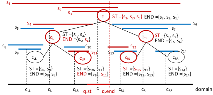
Interval tree. One of the most popular data structures for intervals is Edelsbrunner’s interval tree (Edelsbrunner, 1980), a binary search tree, which takes $O(n)$ space and answers queries in $O(\log n+K)$ time ($K$ is the number of query results). The tree divides the domain hierarchically by placing all intervals strictly before (after) the domain’s center to the left (right) subtree and all intervals that overlap with the domain’s center at the root. This process is repeated recursively for the left and right subtrees using the centers of the corresponding sub-domains. The intervals assigned to each tree node are sorted in two lists based on their starting and ending values, respectively. Interval trees are used to answer stabbing and interval (i.e., range) queries. For example, Figure 1 shows a set of 14 intervals $s_{1},\ldots,s_{14}$, which are assigned to 7 interval tree nodes and a query interval $q=[q.st,q,end]$. The domain point $c$ corresponding to the tree’s root is contained in the query interval, hence all intervals in the root are reported and both the left and right children of the root have to be visited recursively. Since the left child’s point $c_{L}$ is before $q.st$, we access the END list from the end and report results until we find an interval $s$ for which $s.end<q.st$; then we access recursively the right child of $c_{L}$. This process is repeated symmetrically for the root’s right child $c_{R}$. The main drawback of the interval tree is that we need to perform comparisons for most of the intervals in the query result. In addition, updates on the tree can be slow because the lists at each node should be kept sorted. A relational interval tree for disk-resident data was proposed in (Kriegel et al., 2000).

Figure 1. Example of an interval tree

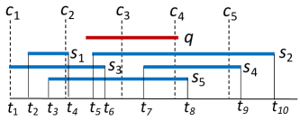
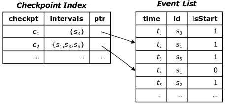
Timeline index. The timeline index (Kaufmann et al., 2013) is a general-purpose access method for temporal (versioned) data, implemented in SAP-HANA. It keeps the endpoints of all intervals in an event list, which is a table of $\langle time,id,isStart\rangle$ triples, where $time$ is the value of the start or end point of the interval, $id$ is the identifier of the interval, and $isStart$ 1 or 0, depending on whether $time$ corresponds to the start or end of the interval, respectively. The event list is sorted primarily by $time$ and secondarily by $isStart$ (descending). In addition, at certain timestamps, called checkpoints, the entire set of active object-ids is materialized, that is the intervals that contain the checkpoint. For each checkpoint, there is a link to the first triple in the event list for which $isStart$=0 and $time$ is greater than or equal to the checkpoint, Figure 2(a) shows a set of five intervals ($s_{1},\ldots,s_{5}$) and Figure 2(b) exemplifies a timeline index for them.

To evaluate a range query (called time-travel query in (Kaufmann et al., 2013)), we first find the largest checkpoint which is smaller than or equal to $q.st$ (e.g., $c_{2}$ in Figure 2) and initialize $R$ as the active interval set at the checkpoint (e.g., $R=\{s_{1},s_{3},s_{5}\}$). Then, we scan the event list from the position pointed by the checkpoint, until the first triple for which $time\geq q.st$, and update $R$ by inserting to it intervals corresponding to an $isStart=1$ event and deleting the ones corresponding to a $isStart=0$ triple (e.g., $R$ becomes $\{s_{3},s_{5}\}$). When we reach $q.st$, all intervals in $R$ are guaranteed query results and they are reported. We continue scanning the event list until the first triple after $q.end$ and we add to the result the ids of all intervals corresponding to triples with $isStart=1$ (e.g., $s_{2}$ and $s_{4}$).

(a) set of intervals	timeline index

Figure 2. Example of a timeline index

The timeline index accesses more data and performs more comparisons than necessary, during range query evaluation. The index also requires a lot of extra space to store the active sets of the checkpoints. Finally, ad-hoc updates are expensive because the event list should be kept sorted.

1D-grid. A simple and practical data structure for intervals is a 1D-grid, which divides the domain into $p$ partitions $P_{1},P_{2},\dots,P_{p}$. The partitions are pairwise disjoint in terms of their interval span and collectively cover the entire data domain $D$. Each interval is assigned to all partitions that it overlaps with. Figure 3 shows 5 intervals assigned to $p=4$ partitions; $s_{1}$ goes to $P_{1}$ only, whereas $s_{5}$ goes to all four partitions. Given a range query $q$, the results can be obtained by accessing each partition $P_{i}$ that overlaps with $q$. For each $P_{i}$ which is contained in $q$ (i.e., $q.st\leq P_{i}.st\wedge P_{i}.end\leq q.end$), all intervals in $P_{i}$ are guaranteed to overlap with $q$. For each $P_{i}$, which overlaps with $q$, but is not contained in $q$, we should compare each $s_{i}\in P_{i}$ with $q$ to determine whether $s_{i}$ is a query result. If the interval of a range query $q$ overlaps with multiple partitions, duplicate results may be produced. An efficient approach for handling duplicates is the reference value method (Dittrich and Seeger, 2000), which was originally proposed for rectangles but can be directly applied for 1D intervals. For each interval $s$ found to overlap with $q$ in a partition $P_{i}$, we compute $v=\max\{s.st,q.st\}$ as the reference value and report $s$ only if $v\in[P_{i}.st,P_{i}.end]$. Since $v$ is unique, $s$ is reported only in one partition. In Figure 3, interval $s_{4}$ is reported only in $P_{2}$ which contains value $\max\{s_{4}.st,q.st\}$.

The 1D-grid has two drawbacks. First, the duplicate results should be computed and checked before being eliminated by the reference value. Second, if the collection contains many long intervals, the index may grow large in size due to excessive replication which increases the number of duplicate results to be eliminated. In contrast, 1D-grid supports fast updates as the partitions are stored independently with no need to organize the intervals in them.

Figure 3. Example of a 1D-grid

Period index. The period index (Behrend et al., 2019) is a domain-partitioning self-adaptive structure, specialized for range and duration queries. The time domain is split into coarse partitions as in a 1D-grid and then each partition is divided hierarchically, in order to organize the intervals assigned to the partition based on their positions and durations. Figure 4 shows a set of intervals and how they are partitioned in a period index. There are two primary partitions $P_{1}$ and $P_{2}$ and each of them is divided hierarchically to three levels. Each level corresponds to a duration length and each interval is assigned to the level corresponding to its duration. The top level stores intervals shorter than the length of a division there, the second level stores longer intervals but shorter than a division there, and so on. Hence, each interval is assigned to at most two divisions, except for intervals which are assigned to the bottom-most level, which can go to an arbitrary number of divisions. During query evaluation, only the divisions that overlap the query range are accessed; if the query carries a duration predicate, the divisions that are shorter than the query duration are skipped. For range queries, the period index performs in par with the interval tree and the 1D-grid (Behrend et al., 2019), so we also compare against this index in Section 5.

Figure 4. Example of a period index

Other works. Another classic data structure for intervals is the segment tree (de Berg et al., 2008), a binary search tree, which has $O(n\log n)$ space complexity and answers stabbing queries in $O(\log n+K)$ time. The segment tree is not designed for range queries, for which it requires a duplicate result elimination mechanism. In computational geometry (de Berg et al., 2008), indexing intervals has been studied as a subproblem within orthogonal 2D range search, and the worst-case optimal interval tree is typically used. Indexing intervals has re-gained interest with the advent of temporal databases (Böhlen et al., 2017). For temporal data, a number of indices are proposed for secondary memory, mainly for effective versioning and compression (Becker et al., 1996; Lomet et al., 2008). Such indexes are tailored for historical versioned data, while we focus on arbitrary interval sets, queries, and updates.

Additional research on indexing intervals does not address range queries, but other operations such as temporal aggregation (Kline and Snodgrass, 1995; Moon et al., 2003; Kaufmann et al., 2013) and interval joins (Dignös et al., 2014; Piatov et al., 2016; Bouros and Mamoulis, 2017; Bouros et al., 2020, 2021; Piatov et al., 2021; Cafagna and Böhlen, 2017; Chekol et al., 2019; Zhu et al., 2019). The timeline index (Kaufmann et al., 2013) can be directly used for temporal aggregation. Piatov et al. (Piatov and Helmer, 2017) present a collection of plane-sweep algorithms that extend the timeline index to support aggregation over fixed intervals, sliding window aggregates, and MIN/MAX aggregates. The timeline index was later adapted for interval overlap joins (Piatov et al., 2016; Piatov et al., 2021). A domain partitioning technique for parallel processing of interval joins was proposed in (Bouros and Mamoulis, 2017; Bouros et al., 2020, 2021). Alternative partitioning techniques for interval joins were proposed in (Dignös et al., 2014; Cafagna and Böhlen, 2017). Partitioning techniques for interval joins cannot replace interval indices as they are not designed for range queries. Temporal joins considering Allen’s algebra relationships for RDF data were studied in (Chekol et al., 2019). Multi-way interval joins in the context of temporal $k$-clique enumeration were studied in (Zhu et al., 2019). Awad et al. (Awad et al., 2022) define interval events in data streams by events of the same or different types that are observed in succession. Analytical operations based on aggregation or reasoning operations can be used to formulate composite interval events.

3. HINT

In this section, we propose the Hierarchical index for INTervals or HINT, which defines a hierarchical domain decomposition and assigns each interval to at most two partitions per level. The primary goal of the index is to minimize the number of comparisons during query evaluation, while keeping the space requirements relatively low, even when there are long intervals in the collection. HINT applies a smart division of intervals in each partition into two groups, which avoids the production and handling of duplicate query results and minimizes the number of intervals that have to be accessed. In Section 3.1, we present a version of HINT, which avoids comparisons overall during query evaluation, but it is not always applicable and may have high space requirements. Then, Section 3.2 presents HINT^m, the general version of our index, used for intervals in arbitrary domains. Last, Section 3.3 describes our analytical model for setting the $m$ parameter and Section 3.4 discusses updates. Table 2 summarizes the notation used in the paper.

Table 2. Table of notations

notation	description
$s.id,s.st,s.end$	identifier, start, end point of interval $s$
$q=[q.st,q.end]$	query range interval
$prefix(k,x)$	$k$-bit prefix of integer $x$
$P_{\ell,i}$	$i$-th partition at level $\ell$ of HINT/HINTm
$P_{\ell,f}$ ($P_{\ell,l}$)	first (last) partition at level $\ell$ that overlaps with $q$
$P_{\ell,i}^{O}$ ($P_{\ell,i}^{R}$)	sub-partition of $P_{\ell,i}$ with originals (replicas)
$P_{\ell,i}^{O_{in}}$ ($P_{\ell,i}^{O_{aft}}$)	intervals in $P^{O}_{\ell,i}i$ ending inside (after) the partition

3.1. A comparison-free version of HINT

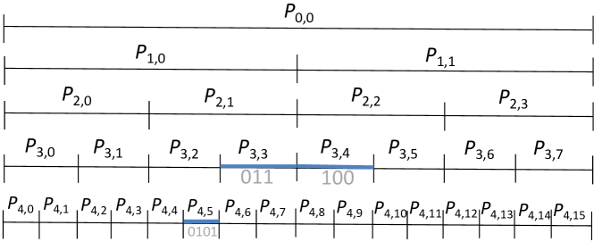
We first describe a version of HINT, which is appropriate in the case of a discrete and not very large domain $D$. Specifically, assume that the domain $D$ wherefrom the endpoints of intervals in $\mathcal{S}$ take value is $[0,2^{m}\!-\!1]$. We can define a regular hierarchical decomposition of the domain into partitions, where at each level $\ell$ from $0$ to $m$, there are $2^{\ell}$ partitions, denoted by array $P_{\ell,0},\dots,P_{\ell,2^{\ell}\!-\!1}$. Figure 5 illustrates the hierarchical domain partitioning for $m=4$.

Each interval $s\in S$ is assigned to the smallest set of partitions which collectively define $s$. It is not hard to show that $s$ will be assigned to at most two partitions per level. For example, in Figure 5, interval $[5,9]$ is assigned to one partition at level $\ell=4$ and two partitions at level $\ell=3$. The assignment procedure is described by Algorithm 1. In a nutshell, for an interval $[a,b]$, starting from the bottom-most level $\ell$, if the last bit of $a$ (resp. $b$) is 1 (resp. 0), we assign the interval to partition $P_{\ell,a}$ (resp. $P_{\ell,b}$) and increase $a$ (resp. decrease $b$) by one. We then update $a$ and $b$ by cutting-off their last bits (i.e., integer division by 2, or bitwise right-shift). If, at the next level, $a>b$ holds, indexing $[a,b]$ is done.

Input : HINT index $\mathcal{H}$, interval $s$

Output : updated $\mathcal{H}$ after indexing $s$

$a\leftarrow s.st$; $b\leftarrow s.end$;

  $\triangleright$ set masks to $s$ endpoints

$\ell\leftarrow m$;

  $\triangleright$ start at the bottom-most level

1 while $\ell\geq 0$ and $a\leq b$ do

2       if last bit of $a$ is $1$ then

             add $s$ to $\mathcal{H}.P_{\ell,a}$;

              $\triangleright$ update partition

3             $a\leftarrow a+1$;

4            

5      if last bit of $b$ is $0$ then

             add $s$ to $\mathcal{H}.P_{\ell,b}$;

              $\triangleright$ update partition

6             $b\leftarrow b-1$;

7            

      $a\leftarrow a\div 2$; $b\leftarrow b\div 2$;

        $\triangleright$ cut-off last bit

       $\ell\leftarrow\ell-1$;

        $\triangleright$ repeat for previous level

8      

ALGORITHM 1 Assignment of an interval to partitions

Figure 5. Hierarchical partitioning and assignment of $[5,9]$

3.1.1. Range queries

A range query $q$ can be evaluated by finding at each level the partitions that overlap with $q$. Specifically, the partitions that overlap with the query interval $q$ at level $\ell$ are partitions $P_{\ell,prefix(\ell,q.st)}$ to $P_{\ell,prefix(\ell,q.end)}$, where $prefix(k,x)$ denotes the $k$-bit prefix of integer $x$. We call these partitions relevant to the query $q$. All intervals in the relevant partitions are guaranteed to overlap with $q$ and intervals in none of these partitions cannot possibly overlap with $q$. However, since the same interval $s$ may exist in multiple partitions that overlap with a query, $s$ may be reported multiple times in the query result.

We propose a technique that avoids the production and therefore, the need for elimination of duplicates and, at the same time, minimizes the number of data accesses. For this, we divide the intervals in each partition $P_{\ell,i}$ into two groups: originals $P^{O}_{\ell,i}$ and replicas $P^{R}_{\ell,i}$. Group $P^{O}_{\ell,i}$ contains all intervals $s\in P_{\ell,i}$ that begin at $P_{\ell,i}$ i.e., $prefix(\ell,s.st)=i$. Group $P^{R}_{\ell,i}$ contains all intervals $s\in P_{\ell,i}$ that begin before $P_{\ell,i}$, i.e., $prefix(\ell,s.st)\neq i$. Each interval is added as original in only one partition of HINT. For example, interval $[5,9]$ in Figure 5 is added to $P^{O}_{4,5}$, $P^{R}_{3,3}$, and $P^{R}_{3,4}$.

Given a range query $q$, at each level $\ell$ of the index, we report all intervals in the first relevant partition $P_{\ell,f}$ (i.e., $P^{O}_{\ell,f}\cup P^{R}_{\ell,f}$). Then, for every other relevant partition $P_{\ell,i}$, $i>f$, we report all intervals in $P^{O}_{\ell,i}$ and ignore $P^{R}_{\ell,i}$. This guarantees that no result is missed and no duplicates are produced. The reason is that each interval $s$ will appear as original in just one partition, hence, reporting only originals cannot produce any duplicates. At the same time, all replicas $P^{R}_{\ell,f}$ in the first partitions per level $\ell$ that overlap with $q$ begin before $q$ and overlap with $q$, so they should be reported. On the other hand, replicas $P^{R}_{\ell,i}$ in subsequent relevant partitions ($i>f$) contain intervals, which are either originals in a previous partition $P_{\ell,j}$, $j<i$ or replicas in $P^{R}_{\ell,f}$, so, they can safely be skipped. Algorithm 2 describes the range query algorithm using HINT.

Input : HINT index $\mathcal{H}$, query interval $q$

Output : set $\mathcal{R}$ of all intervals that overlap with $q$

1 $\mathcal{R}\leftarrow\emptyset$;

2 foreach level $\ell$ in $\mathcal{H}$ do

3       $p\leftarrow prefix(\ell,q.st)$;

4       $\mathcal{R}\leftarrow\mathcal{R}\cup\{s.id|s\in\mathcal{H}.P^{O}_{\ell,p}\cup\mathcal{H}.P^{R}_{\ell,p}\}$

5       while $p<prefix(\ell,q.end)$ do

6             set $p\leftarrow p+1$;

7             $\mathcal{R}\leftarrow\mathcal{R}\cup\{s.id|s\in\mathcal{H}.P^{O}_{\ell,p}\}$

8            

9      

10return $\mathcal{R}$;

ALGORITHM 2 Range query on HINT

For example, consider the hierarchical partitioning of Figure 6 and a query interval $q=[5,9]$. The binary representations of $q.st$ and $q.end$ are 0101 and 1001, respectively. The relevant partitions at each level are shown in bold (blue) and dashed (red) lines and can be determined by the corresponding prefixes of 0101 and 1001. At each level $\ell$, all intervals (both originals and replicas) in the first partitions $P_{\ell,f}$ (bold/blue) are reported while in the subsequent partitions (dashed/red), only the original intervals are.

Figure 6. Accessed partitions for range query $[5,9]$

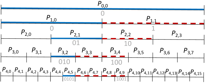
Discussion. The version of HINT described above finds all range query results, without conducting any comparisons. This means that in each partition $P_{\ell,i}$, we only have to keep the ids of the intervals that are assigned to $P_{\ell,i}$ and do not have to store/replicate the interval endpoints. In addition, the relevant partitions at each level are computed by fast bit-shifting operations which are comparison-free. To use HINT for arbitrary integer domains, we should first normalize all interval endpoints by subtracting the minimum endpoint, in order to convert them to values in a $[0,2^{m}-1]$ domain (the same transformation should be applied on the queries). If the required $m$ is very large, we can index the intervals based on their $m$-bit prefixes and support approximate search on discretized data. Approximate search can also be applied on intervals in a real-valued domain, after rescaling and discretization in a similar way.

3.2. HINT^m: indexing arbitrary intervals

We now present a generalized version of HINT, denoted by HINT^m, which can be used for intervals in arbitrary domains. HINT^m uses a hierarchical domain partitioning with $m+1$ levels, based on a $[0,2^{m}-1]$ domain $D$; each raw interval endpoint is mapped to a value in $D$, by linear rescaling. The mapping function $f(\mathbb{R}\to D)$ is $f(x)=\lfloor\frac{x-min(x)}{max(x)-min(x)}\cdot(2^{m}-1)\rfloor$, where $min(x)$ and $max(x)$ are the minimum and maximum interval endpoints in the dataset $S$, respectively. Each raw interval $[s.st,s.end]$ is mapped to interval $[f(s.st),f(s.end)]$. The mapped interval is then assigned to at most two partitions per level in HINT^m, using Algorithm 1.

For the ease of presentation, we will assume that the raw interval endpoints take values in $[0,2^{m^{\prime}}-1]$, where $m^{\prime}>m$, which means that the mapping function $f$ simply outputs the $m$ most significant bits of its input. As an example, assume that $m=4$ and $m^{\prime}=6$. Interval $[21,38]$ (=$[0b010101,0b100110]$) is mapped to interval $[5,9]$ (=$[0b0101,0b1001]$) and assigned to partitions $P_{4,5}$, $P_{3,3}$, and $P_{3,4}$, as shown in Figure 5. So, in contrast to HINT, the set of partitions whereto an interval $s$ is assigned in HINT^m does not define $s$, but the smallest interval in the $[0,2^{m}-1]$ domain $D$, which covers $s$. As in HINT, at each level $\ell$, we divide each partition $P_{\ell,i}$ to $P^{O}_{\ell,i}$ and $P^{R}_{\ell,i}$, to avoid duplicate query results.

3.2.1. Query evaluation using HINT^m

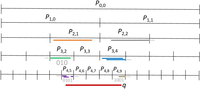
For a range query $q$, simply reporting all intervals in the relevant partitions at each level (as in Algorithm 2) would produce false positives. Instead, comparisons to the query endpoints may be required for the first and the last partition at each level that overlap with $q$. Specifically, we can consider each level of HINT^m as a 1D-grid (see Section 2) and go through the partitions at each level $\ell$ that overlap with $q$. For the first partition $P_{\ell,f}$, we verify whether $s$ overlaps with $q$ for each interval $s\in P^{O}_{\ell,f}$ and each $s\in P^{R}_{\ell,f}$. For the last partition $P_{\ell,l}$, we verify whether $s$ overlaps with $q$ for each interval $s\in P^{O}_{\ell,l}$. For each partition $P_{\ell,i}$ between $P_{\ell,f}$ and $P_{\ell,l}$, we report all $s\in P^{O}_{\ell,i}$ without any comparisons. As an example, consider the HINT^m index and the range query interval $q$ shown in Figure 7. The identifiers of the relevant partitions to $q$ are shown in the figure (and also some indicative intervals that are assigned to these partitions). At level $m=4$, we have to perform comparisons for all intervals in the first relevant partitions $P_{4,5}$. In partitions $P_{4,6}$,…,$P_{4,8}$, we just report the originals in them as results, while in partition $P_{4,9}$ we compare the start points of all originals with $q$, before we can confirm whether they are results or not. We can simplify the overlap tests at the first and the last partition of each level $\ell$ based on the following:

Lemma 0.

At every level $\ell$, each $s\in P^{R}_{\ell,f}$ is a query result iff $q.st\leq s.end$. If $l>f$, each $s\in P^{O}_{\ell,l}$ is a query result iff $s.st\leq q.end$.

Proof.

For the first relevant partition $P_{\ell,f}$ at each level $\ell$, for each replica $s\in P^{R}_{\ell,f}$, $s.st<q.st$, so $q.st\leq s.end$ suffices as an overlap test. For the last partition $P_{\ell,l}$, if $l>f$, for each original $s\in P^{O}_{\ell,f}$, $q.st<s.st$, so $s.st\leq q.end$ suffices as an overlap test. ∎

Figure 7. Avoiding redundant comparisons in HINT^m

3.2.2. Avoiding redundant comparisons in query evaluation

One of our most important findings in this study and a powerful feature of HINT^m is that at most levels, it is not necessary to do comparisons at the first and/or the last partition. For instance, in the previous example, we do not have to perform comparisons for partition $P_{3,4}$, since any interval assigned to $P_{3,4}$ should overlap with $P_{4,8}$ and the interval spanned by $P_{4,8}$ is covered by $q$. This means that the start point of all intervals in $P_{3,4}$ is guaranteed to be before $q.end$ (which is inside $P_{4,9}$). In addition, observe that for any relevant partition which is the last partition at an upper level and covers $P_{3,4}$ (i.e., partitions $\{P_{2,2},P_{1,1},P_{0,0}\}$), we do not have to conduct the $s.st\leq q.end$ tests as intervals in these partitions are guaranteed to start before $P_{4,9}$. The lemma below formalizes these observations:

Lemma 0.

If the first (resp. last) relevant partition for a query $q$ at level $\ell$ ($\ell<m$) starts (resp. ends) at the same value as the first (resp. last) relevant partition at level $\ell+1$, then for every first (resp. last) relevant partition $P_{v,f}$ (resp. $P_{v,l}$) at levels $v\leq\ell$, each interval $s\in P_{v,f}$ (resp. $s\in P_{v,l}$) satisfies $s.end\geq q.st$ (resp. $s.st\leq q.end$).

Proof.

Let $P.st$ (resp. $P.end$) denote the first (resp. last) domain value of partition $P$. Consider the first relevant partition $P_{\ell,f}$ at level $\ell$ and assume that $P_{\ell,f}.st=P_{\ell+1,f}.st$. Then, for every interval $s\in P_{\ell,f}$, $s.end\geq P_{\ell+1,f}.end$, otherwise $s$ would have been allocated to $P_{\ell+1,f}$ instead of $P_{\ell,f}$. Further, $P_{\ell+1,f}.end\geq q.st$, since $P_{\ell+1,f}$ is the first partition at level $\ell+1$ which overlaps with $q$. Hence, $s.end\geq q.st$. Moreover, for every interval $s\in P_{v,f}$ with $v<\ell$, $s.end\geq P_{\ell+1,f}.end$ holds, as interval $P_{v,f}$ covers interval $P_{\ell,f}$; so, we also have $s.end\geq q.st$. Symmetrically, we prove that if $P_{\ell,l}.end=P_{\ell+1,l}.end$, then for each $s\in P_{v,l},v\leq\ell$, $s.st\leq q.end$. ∎

We next focus on how to rapidly check the condition of Lemma 2. Essentially, if the last bit of the offset $f$ (resp. $l$) of the first (resp. last) partition $P_{\ell,f}$ (resp. $P_{\ell,l}$) relevant to the query at level $\ell$ is 0 (resp. 1), then the first (resp. last) partition at level $\ell-1$ above satisfies the condition. For example, in Figure 7, consider the last relevant partition $P_{4,9}$ at level $4$. The last bit of $l=9$ is 1; so, the last partition $P_{3,4}$ at level $3$ satisfies the condition and we do not have to perform comparisons in the last partitions at level $3$ and above.

Algorithm 3 is a pseudocode for the range query algorithm on HINT^m. The algorithm accesses all levels of the index, bottom-up. It uses two auxiliary flag variables $compfirst$ and $complast$ to mark whether it is necessary to perform comparisons at the current level (and all levels above it) at the first and the last partition, respectively, according to the discussion in the previous paragraph. At each level $\ell$, we find the offsets of the relevant partitions to the query, based on the $\ell$-prefixes of $q.st$ and $q.end$ (Line 3). For the first position $f=prefix(q,st)$, the partitions holding originals and replicas $P^{O}_{\ell,f}$ and $P^{R}_{\ell,f}$ are accessed. The algorithm first checks whether $f=l$, i.e., the first and the last partitions coincide. In this case, if $compfirst$ and $complast$ are set, then we perform all comparisons in $P^{O}_{\ell,f}$ and apply the first observation in Lemma 1 to $P^{R}_{\ell,f}$. Else, if only $complast$ is set, we can safely skip the $q.st\leq s.end$ comparisons; if only $compfist$ is set, regardless whether $f=l$, we just perform $q.st\leq s.end$ comparisons to both originals and replicas to the first partition. Finally, if neither $compfirst$ nor $complast$ are set, we just report all intervals in the first partition as results. If we are at the last partition $P_{\ell,l}$ and $l>f$ (Line 17) then we just examine $P^{O}_{\ell,l}$ and apply just the $s.st\leq q.end$ test for each interval there, according to Lemma 1. Finally, for all partitions in-between the first and the last one, we simply report all original intervals there.

Input : HINT^m index $\mathcal{H}$, query interval $q$

Output : set $\mathcal{R}$ of intervals that overlap with $q$

1 $compfirst\leftarrow TRUE$; $complast\leftarrow TRUE$;

2 $\mathcal{R}\leftarrow\emptyset$;

3 for $\ell=m$ to $0$ do $\triangleright$ bottom-up

4       $f\leftarrow prefix(\ell,q.st)$; $l\leftarrow prefix(\ell,q.end)$;

5       for $i=f$ to $l$ do

6             if $i=f$ then $\triangleright$ first overlapping partition

7                   if $i=l$ and $compfirst$ and $complast$ then

8                         $\mathcal{R}\leftarrow\mathcal{R}\cup\{s.id|s\in\mathcal{H}.P^{O}_{\ell,i},q.st\leq s.end\land s.st\leq q.end\}$;

9                         $\mathcal{R}\leftarrow\mathcal{R}\cup\{s.id|s\in\mathcal{H}.P^{R}_{\ell,i},q.st\leq s.end\}$;

10                        

11                  else if $i=l$ and $complast$ then

12                         $\mathcal{R}\leftarrow\mathcal{R}\cup\{s.id|s\in\mathcal{H}.P^{O}_{\ell,i},s.st\leq q.end\}$;

13                         $\mathcal{R}\leftarrow\mathcal{R}\cup\{s.id|s\in\mathcal{H}.P^{R}\}$;

14                        

15                  else if $compfirst$ then

16                         $\mathcal{R}\leftarrow\mathcal{R}\cup\{s.id|s\in\mathcal{H}.P^{O}_{\ell,i}\cup\mathcal{H}.P^{R}_{\ell,i},q.st\leq s.end\}$;

17                        

18                  else

19                         $\mathcal{R}\leftarrow`\mathcal{R}\cup\{s.id|s\in\mathcal{H}.P^{O}_{\ell,i}\cup\mathcal{H}.P^{R}_{\ell,i}\}$;

20                        

21                  

22            else if $i=l$ and $complast$ then $\triangleright$ last partition, $l>f$

23                   $\mathcal{R}\leftarrow\mathcal{R}\cup\{s.id|s\in\mathcal{H}.P^{O}_{\ell,i},s.st\leq q.end\}$;

24                  

25            else  $\triangleright$ in-between or last ($l>f$), no comparisons

26                   $\mathcal{R}\leftarrow\mathcal{R}\cup\{s.id|s\in\mathcal{H}.P^{O}_{\ell,i}\}$;

27                  

28            

29      if $f~{}\textrm{mod}~{}2=0$ then $\triangleright$ last bit of $f$ is 0

30            $compfirst\leftarrow FALSE$;

31      if $l~{}\textrm{mod}~{}2=1$ then $\triangleright$ last bit of $l$ is 1

32            $complast\leftarrow FALSE$;

33      

34return $\mathcal{R}$;

ALGORITHM 3 Range query on HINT^m

3.2.3. Complexity Analysis

Let $n$ be the number of intervals in $\mathcal{S}$. Assume that the domain is $[0,2^{m^{\prime}}-1]$, where $m^{\prime}>m$. To analyze the space complexity of HINT^m, we first prove the following lemma:

Lemma 0.

The total number of intervals assigned at the lowest level $m$ of HINT^m is expected to be $n$.

Proof.

Each interval $s\in\mathcal{S}$ will go to zero, one, or two partitions at level $m$, based on the bits of $s.st$ and $s.end$ at position $m$ (see Algorithm 1); on average, $s$ will go to one partition. ∎

Using Algorithm 1, when an interval is assigned to a partition at a level $\ell$, the interval is truncated (i.e., shortened) by $2^{m^{\prime}-\ell}$. Based on this, we analyze the space complexity of HINT^m as follows.

Theorem 4.

Let $\lambda$ be the average length of intervals in input collection $S$. The space complexity of HINT^m is $O(n\cdot\log_{2}(2^{\log_{2}\lambda-m^{\prime}+m}+1))$.

Proof.

Based on Lemma 3, each $s\in S$ will be assigned on average to one partition at level $m$ and will be truncated by $2^{m^{\prime}-m}$. Following Algorithm 1, at the next level $m-1$, $s$ is also be expected to be assigned to one partition (see Lemma 3) and truncated by $2^{m^{\prime}-m+1}$, and so on, until the entire interval is truncated (condition $a\leq b$ is violated at Line 3 of Algorithm 1). Hence, we are looking for the number of levels whereto each $s$ will be assigned, or for the smallest $k$ for which $2^{m^{\prime}-m}+2^{m^{\prime}-m+1}+\dots+2^{m^{\prime}-m+k-1}\geq\lambda$. Solving the inequality gives $k\geq\log_{2}(2^{\log_{2}\lambda-m^{\prime}+m}+1)$ and the space complexity of HINT^m is $O(n\cdot k)$ ∎

For the computational cost of range queries in terms of conducted comparisons, in the worst case, $O(n)$ intervals are assigned to the first relevant partition $P_{m,f}$ at level $m$ and $O(n)$ comparisons are required. To estimate the expected cost of range query evaluation in terms of conducted comparisons, we assume a uniform distribution of intervals to partitions and random query intervals.

Lemma 0.

The expected number of HINT^m partitions for which we have to conduct comparisons is four.

Proof.

At the last level of the index $m$, we definitely have to do comparisons in the first and the last partition (which are different in the worst case). At level $m-1$, for each of the first and last partitions, we have a 50% chance to avoid comparisons, due to Lemma 2. Hence, the expected number of partitions for which we have to perform comparisons at level $m-1$ is 1. Similarly, at level $m-2$ each of the yet active first/last partitions has a 50% chance to avoid comparisons. Overall, for the worst-case conditions, where $m$ is large and $q$ is long, the expected number of partitions, for which we need to perform comparisons is $2+1+0.5+0.25+\dots=4$. ∎

Theorem 6.

The expected number of comparisons during query evaluation over HINT^m is $O(n/2^{m})$.

Proof.

For each query, we expect to conduct comparisons at least in the first and the last relevant partitions at level $m$. The expected number of intervals, in each of these two partitions, is $O(n/2^{m})$, considering Lemma 3 and assuming a uniform distribution of the intervals in the partitions. In addition, due to Lemma 5, the number of expected additional partitions that require comparisons is 2 and each of these two partitions is expected to also hold at most $O(n/2^{m})$ intervals, by Lemma 3 on the levels above $m$ and using the truncated intervals after their assignment to level $m$ (see Algorithm 1). Hence, $q$ is expected to be compared with $O(n/2^{m})$ intervals in total and the cost of each such comparison is $O(1)$. ∎

3.3. Setting $m$

As shown in Section 3.2.3, the space requirements and the search performance of HINT^m depend on the value of $m$. For large values of $m$, the cost of accessing comparison-free results will dominate the computational cost of comparisons. This section presents an analytical study for estimating $m_{opt}$: the smallest value of $m$, which is expected to result in a HINT^m of search performance close to the best possible, while achieving the lowest possible space requirements. Our study uses simple statistics namely, the number of intervals $n=|\mathcal{S}|$, the mean length $\lambda_{s}$ of data intervals and the mean length $\lambda_{q}$ of query intervals. We assume that the endpoints and the lengths of both intervals and queries are uniformly distributed.

The overall cost of query evaluation consists of (1) the cost for determining the relevant partitions per level, denoted by $C_{p}$, (2) the cost of conducting comparisons between data intervals and the query, denoted by $C_{cmp}$, and (3) the cost of accessing query results in the partitions for which we do not have to conduct comparisons, denoted by $C_{acc}$. Cost $C_{p}$ is negligible, as the partitions are determined by a small number $m$ of bit-shifting operations. To estimate $C_{cmp}$, we need to estimate the number of intervals in the partitions whereat we need to conduct comparisons and multiply this by the expected cost $\beta_{cmp}$ per comparison. To estimate $C_{acc}$, we need to estimate the number of intervals in the corresponding partitions and multiply this by the expected cost $\beta_{acc}$ of (sequentially) accessing and reporting one interval. $\beta_{cmp}$ and $\beta_{acc}$ are machine-dependent and can easily be estimated by experimentation.

According to Algorithm 3, unless $\lambda_{q}$ is smaller than the length of a partition at level $m$, there will be two partitions that require comparisons at level $m$, one partition at level $m-1$, etc. with the expected number of partitions being at most four (see Lemma 5). Hence, we can assume that $C_{cmp}$ is practically dominated by the cost of processing two partitions at the lowest level $m$. As each partition at level $m$ is expected to have $n/2^{m}$ intervals (see Lemma 3), we have $C_{cmp}=\beta_{cmp}\cdot n/2^{m}$. Then, the number of accessed intervals for which we expect to apply no comparisons is $|Q|-2\cdot n/2^{m}$, where $|Q|$ is the total number of expected query results. Under this, we have $C_{acc}=\beta_{acc}\cdot(|Q|-2\cdot n/2^{m})$. We can estimate $|Q|$ using the selectivity analysis for (multidimensional) intervals and range queries in (Pagel et al., 1993) as $|Q|=n\cdot\frac{\lambda_{s}+\lambda_{q}}{\Lambda}$, where $\Lambda$ is the length of the entire domain with all intervals in $\mathcal{S}$ (i.e., $\Lambda=\max_{\forall s\in\mathcal{S}}s.end-\min_{\forall s\in\mathcal{S}}s.st$).

With $C_{cmp}$ and $C_{acc}$, we now discuss how to estimate $m_{opt}$. First, we gradually increase $m$ from $1$ up to its max value $m^{\prime}$ (determined by $\Lambda$), and compute the expected cost $C_{cmp}+C_{acc}$. For $m=m^{\prime}$, HINT^m corresponds to the comparison-free HINT with the lowest expected cost. Then, we select as $m_{opt}$ the lowest value of $m$ for which $C_{cmp}+C_{acc}$ converges to the cost of the $m=m^{\prime}$ case.

3.4. Updates

We handle insertions to an existing HINT or HINT^m index by calling Algorithm 1 for each new interval $s$. Small adjustments are needed for HINT^m to add $s$ to the originals division at the first partition assignment, i.e., to $P^{O}_{\ell,a}$ or $P^{O}_{\ell,b}$, and to the replicas division for every other partition, i.e., to $P^{R}_{\ell,a}$ or $P^{R}_{\ell,b}$ Finally, we handle deletions using tombstones, similarly to previous studies (Lomet, 1975; Overmars, 1983) and recent indexing approaches (Ferragina and Vinciguerra, 2020). Given an interval $s$ for deletion, we first search the index to locate all partitions that contain $s$ (both as original and as replica) and then, replace the id of $s$ by a special “tombstone” id, which signals the logical deletion.

4. Optimizing HINT^m

In this section, we discuss optimization techniques, which greatly improve the performance of HINT^m (and HINT) in practice. First, we show how to reduce the number of partitions in HINT^m where comparisons are performed and how to avoid accessing unnecessary data. Next, we show how to handle very sparse or skewed data at each level of HINT/HINT^m. Another (orthogonal) optimization is decoupling the storage of the interval ids with the storage of interval endpoints in each partition. Finally, we revisit updates under the prism of these optimizations.

4.1. Subdivisions and space decomposition

Recall that, at each level $\ell$ of HINT^m, every partition $P_{\ell,i}$ is divided into $P^{O}_{\ell,i}$ (holding originals) and $P^{R}_{\ell,i}$ (holding replicas). We propose to further divide each $P^{O}_{\ell,i}$ into $P^{O_{in}}_{\ell,i}$ and $P^{O_{aft}}_{\ell,i}$, so that $P^{O_{in}}_{\ell,i}$ (resp. $P^{O_{aft}}_{\ell,i}$) holds the intervals from $P^{O_{in}}_{\ell,i}$ that end inside (resp. after) partition $P_{\ell,i}$. Similarly, each $P_{\ell,i}^{R}$ is divided into $P_{\ell,i}^{R_{in}}$ and $P_{\ell,i}^{R_{aft}}$.

Range queries that overlap with multiple partitions. Consider a range query $q$, which overlaps with a sequence of more than one partitions at level $\ell$. As already discussed, if we have to conduct comparisons in the first such partition $P_{\ell,f}$, we should do so for all intervals in $P_{\ell,f}^{O}$ and $P_{\ell,f}^{R}$. By subdividing $P_{\ell,f}^{O}$ and $P_{\ell,f}^{R}$, we get the following lemma:

Lemma 0.

If $P_{\ell,f}\neq P_{\ell,l}$ (1) each interval $s$ in $P_{\ell,f}^{O_{in}}\cup P_{\ell,f}^{R_{in}}$ overlaps with $q$ iff $s.end\geq q.st$; and (2) all intervals $s$ in $P_{\ell,f}^{O_{aft}}$ and $P_{\ell,f}^{R_{aft}}$ are guaranteed to overlap with $q$.

Proof.

Follows directly from the fact that $q$ starts inside $P_{\ell,f}$ but ends after $P_{\ell,f}$. ∎

Hence, we need just one comparison for each interval in $P_{\ell,f}^{O_{in}}\cup P_{\ell,f}^{R_{in}}$, whereas we can report all intervals $P_{\ell,f}^{O_{aft}}\cup P_{\ell,f}^{R_{aft}}$ as query results without any comparisons. As already discussed, for all partitions $P_{\ell,i}$ between $P_{\ell,f}$ and $P_{\ell,l}$, we just report intervals in $P_{\ell,i}^{O_{in}}\cup P_{\ell,i}^{O_{aft}}$ as results, without any comparisons, whereas for the last partition $P_{\ell,l}$, we perform one comparison per interval in $P_{\ell,l}^{O_{in}}\cup P_{\ell,l}^{O_{aft}}$.

Range queries that overlap with a single partition. If the range query $q$ overlaps only one partition $P_{\ell,f}$ at level $\ell$, we can use following lemma to minimize the necessary comparisons:

Lemma 0.

If $P_{\ell,f}=P_{\ell,l}$ then

• each interval $s$ in $P_{\ell,f}^{O_{in}}$ overlaps with $q$ iff $s.st\leq q.end\wedge q.st\leq s.end$,

• each interval $s$ in $P_{\ell,f}^{O_{aft}}$ overlaps with $q$ iff $s.st\leq q.end$,

• each interval $s$ in $P_{\ell,f}^{R_{in}}$ overlaps with $q$ iff $s.end\geq q.st$,

• all intervals in $P_{\ell,f}^{R_{aft}}$ overlap with $q$.

Proof.

All intervals $s\in P_{\ell,f}^{O_{aft}}$ end after $q$, so $s.st\leq q.end$ suffices as an overlap test. All intervals $s\in P_{\ell,f}^{R_{in}}$ start before $q$, so $s.st\leq q.end$ suffices as an overlap test. All intervals $s\in P_{\ell,f}^{R_{aft}}$ start before and end after $q$, so they are guaranteed results. ∎

Figure 8. Partition subdivisions in HINT^m (level $\ell=2$)

Overall, the subdivisions help us to minimize the number of intervals in each partition, for which we have to apply comparisons. Figure 8 shows the subdivisions which are accessed by query $q$ at level $\ell=2$ of a HINT^m index. In partition $P_{\ell,f}=P_{2,1}$, all four subdivisions are accessed, but comparisons are needed only for intervals in $P_{2,1}^{O_{in}}$ and $P_{2,1}^{R_{in}}$. In partition $P_{2,2}$, only the originals (in $P_{2,2}^{O_{in}}$ and $P_{2,2}^{O_{aft}}$) are accessed and reported without any comparisons. Finally, in $P_{\ell,l}=P_{2,3}$, only the originals (in $P_{2,3}^{O_{in}}$ and $P_{2,3}^{O_{aft}}$) are accessed and compared to $q$.

4.1.1. Sorting the intervals in each subdivision

We can keep the intervals in each subdivision sorted, in order to reduce the number of comparisons for queries that access them. For example, let us examine the last partition $P_{\ell,l}$ that overlaps with a query $q$ at a level $\ell$. If the intervals $s$ in $P_{\ell,l}^{O_{in}}$ are sorted on their start endpoint (i.e., $s.st$), we can simply access and report the intervals until the first $s\in P_{\ell,l}^{O_{in}}$, such that $s.st>q.end$. Or, we can perform binary search to find the first $s\in P_{\ell,l}^{O_{in}}$, such that $s.st>q.end$ and then scan and report all intervals before $s$. Table 3 (second column) summarizes the sort orders for each of the four subdivisions of a partition that can be beneficial in range query evaluation. For a subdivision $P_{\ell,i}^{O_{in}}$, intervals may have to be compared based on their start point (if $P_{\ell,i}=P_{\ell,f}$), or based on their end point (if $P_{\ell,i}=P_{\ell,l}$), or based on both points (if $P_{\ell,i}=P_{\ell,f}=P_{\ell,l}$). Hence, we choose to sort based on either $s.st$ or $s.end$ to accommodate two of these three cases. For a subdivision $P_{\ell,i}^{O_{aft}}$, intervals may only have to be compared based on their start point (if $P_{\ell,i}=P_{\ell,l}$). For a subdivision $P_{\ell,i}^{R_{in}}$, intervals may only have to be compared based on their end point (if $P_{\ell,i}=P_{\ell,f}$). Last, for a subdivision $P_{\ell,i}^{R_{aft}}$, there is never any need to compare the intervals, so, no order provides any search benefit.

Table 3. Sort orders that can be beneficial

subdivision	beneficial sorting	necessary data
$P_{\ell,i}^{O_{in}}$	by $s.st$ or by $s.end$	$s.id,s.st,s.end$
$P_{\ell,i}^{O_{aft}}$	by $s.st$	$s.id,s.st$
$P_{\ell,i}^{R_{in}}$	by $s.end$	$s.id,s.end$
$P_{\ell,i}^{R_{aft}}$	no sorting	$s.id$

4.1.2. Storage optimization

So far, we have assumed that each interval $s$ is stored in the partitions whereto $s$ is assigned as a triplet $\langle s.id,s.st,s.end\rangle$. However, if we split the partitions into subdivisions, we do not need to keep all information of the intervals in them. Specifically, for each subdivision $P_{\ell,i}^{O_{in}}$, we may need to use $s.st$ and/or $s.end$ for each interval $s\in P_{\ell,i}^{O_{in}}$, while for each subdivision $P_{\ell,i}^{O_{aft}}$, we may need to use $s.st$ for each $s\in P_{\ell,i}^{O_{in}}$, but we will never need $s.end$. From the intervals $s$ of each subdivision $P_{\ell,i}^{R_{in}}$, we may need $s.end$, but we will never use $s.st$. Finally, for each subdivision $P_{\ell,i}^{R_{in}}$, we just have to keep the $s.id$ identifiers of the intervals. Table 3 (third column) summarizes the data that we need to keep from each interval in the subdivisions of each partition. Since each interval $s$ is stored as original just once in the entire index, but as replica in possibly multiple partitions, space can be saved by storing only the necessary data, especially if the intervals span multiple partitions. Last, note that even when we do not apply the subdivisions, but just use divisions $P_{\ell,i}^{O}$ and $P_{\ell,i}^{R}$ (as suggested in Section 3.2), we do not have to store the start points $s.st$ of all intervals in $P_{\ell,i}^{R}$, since they are never used in comparisons.

4.2. Handling data skewness and sparsity

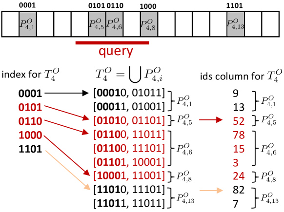
Data skewness and sparsity may cause many partitions to be empty, especially at the lowest levels of HINT (i.e., large values of $\ell$). Recall that a query accesses a sequence of multiple $P^{O}_{\ell,i}$ partitions at each level $\ell$. Since the intervals are physically distributed in the partitions, this results into the unnecessary accessing of empty partitions and may cause cache misses. We propose a storage organization where all $P_{\ell,i}^{O}$ divisions at the same level $\ell$ are merged into a single table $T_{\ell}^{O}$ and an auxiliary index is used to find each non-empty division. The auxiliary index locates the first non-empty partition, which is greater than or equal to the $\ell$-prefix of $q.st$ (i.e., via binary search or a binary search tree). From thereon, the nonempty partitions which overlap with the query interval are accessed sequentially and distinguished with the help of the auxiliary index. Hence, the contents of the relevant $P^{O}_{\ell,i}$’s to each query are always accessed sequentially. Figure 9(a) shows an example at level $\ell=4$ of HINT^m. From the total $2^{\ell}=16$ $P^{O}$ partitions at that level, only 5 are nonempty (shown in grey at the top of the figure): $P^{O}_{4,1},P^{O}_{4,5},P^{O}_{4,6},P^{O}_{4,8},P^{O}_{4,13}$. All 9 intervals in them (sorted by start point) are unified in a single table $T_{4}^{O}$ as shown at the bottom of the figure (the binary representations of the interval endpoints are shown). At the moment, ignore the ids column for $T_{4}^{O}$ at the right of the figure. The sparse index for $T_{4}^{O}$ has one entry per nonempty partition pointing to the first interval in it. For the query in the example, the index is used to find the first nonempty partition $P^{O}_{4,5}$, for which the id is greater than or equal to the $4$-bit prefix $0100$ of $q.st$. All relevant non-empty partitions $P^{O}_{4,5},P^{O}_{4,6},P^{O}_{4,8}$ are accessed sequentially from $T_{4}^{O}$, until the position of the first interval of $P^{O}_{4,13}$.

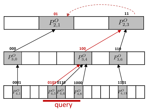
Searching for the first partition $P^{O}_{\ell,f}$ that overlaps with $q$ at each level can be quite expensive when numerous nonempty partitions exist. To alleviate this issue, we suggest adding to the auxiliary index, a link from each partition $P^{O}_{\ell,i}$ to the partition $P^{O}_{\ell-1,j}$ at the level above, such that $j$ is the smallest number greater than or equal to $i\div 2$, for which partition $P^{O}_{\ell-1,j}$ is not empty. Hence, instead of performing binary search at level $\ell-1$, we use the link from the first partition $P^{O}_{\ell,f}$ relevant to the query at level $\ell$ and (if necessary) apply a linear search backwards starting from the pointed partition $P^{O}_{\ell-1,j}$ to identify the first non-empty partition $P^{O}_{\ell-1,f}$ that overlaps with $q$. Figure 9(b) shows an example, where each nonempty partition at level $\ell$ is linked with the first nonempty partition with greater than or equal prefix at the level $\ell-1$ above. Given query example $q$, we use the auxiliary index to find the first nonempty partition $P^{O}_{4,5}$ which overlaps with $q$ and also sequentially access $P^{O}_{4,6}$ and $P^{O}_{4,8}$. Then, we follow the pointer from $P^{O}_{4,5}$ to $P^{O}_{3,4}$ to find the first nonempty partition at level $3$, which overlaps with $q$. We repeat this to get partition $P^{O}_{2,3}$ at level $2$, which however is not guaranteed to be the first one overlapping with $q$, so we go backwards to $P^{O}_{2,3}$.

(a) auxiliary index

(b) linking between levels

Figure 9. Storage and indexing optimizations

4.3. Reducing cache misses

At most levels of HINT^m, no comparisons are conducted and the only operations are processing the interval ids which qualify the query. In addition, even for the levels $\ell$ where comparisons are required, these are only restricted to the first and the last partitions $P^{O}_{\ell,f}$ and $P^{O}_{\ell,l}$ that overlap with $q$ and no comparisons are needed for the partitions that are in-between. Summing up, when accessing any (sub-)partition for which no comparison is required, we do not need any information about the intervals, except for their ids. Hence, in our implementation, for each (sub-)partition, we store the ids of all intervals in it in a dedicated array (the ids column) and the interval endpoints (wherever necessary) in a different array. If we need the id of an interval that qualifies a comparison, we can access the corresponding position of the ids column. This storage organization greatly improves search performance by reducing the cache misses, because for the intervals that do not require comparisons, we only access their ids and not their interval endpoints. This optimization is orthogonal to and applied in combination with the strategy discussed in Section 4.2, i.e., we store all $P^{O}$ divisions at each level $\ell$ in a single table $T_{\ell}^{O}$, which is decomposed to a column that stores the ids and another table for the endpoint data of the intervals. An example of the ids column is shown in Figure 9(a). If, for a sequence of partitions at a level, we do not have to perform any comparisons, we just access the sequence of the interval ids that are part of the answer, which is implied by the position of the first such partition (obtained via the auxiliary index). In this example, all intervals in $P^{O}_{4,5}$ and $P^{O}_{4,6}$ are guaranteed to be query results without any comparisons and they can be sequentially accessed from the ids column without having to access the endpoints of the intervals. The auxiliary index guides the search by identifying and distinguishing between partitions for which comparisons should be conducted (e.g., $P^{O}_{4,8}$) and those for which they are not necessary.

4.4. Updates

A version of HINT^m that uses all techniques from Sections 4.1-4.2, is optimized for query operations. Under this premise, the index cannot efficiently support individual updates, i.e., new intervals inserted one-by-one. Dealing with updates in batches will be a better fit. This is a common practice for other update-unfriendly indices, e.g., the inverted index in IR. Yet, for mixed workloads (i.e., with both queries and updates), we adopt a hybrid setting where a delta index is maintained to digest the latest updates as discussed in Section 3.4, and a fully optimized HINT^m, which is updated periodically in batches, holds older data supporting deletions with tombstones. Both indices are probed when a query is evaluated.

5. Experimental Analysis

We compared our hierarchical index, detailed in Sections 3 and 4 against the interval tree (Edelsbrunner, 1980) (code from (Garrison, [n.d.])), the timeline index (Kaufmann et al., 2013), the (adaptive) period index (Behrend et al., 2019), and a uniform 1D-grid. All indices were implemented in C++ and compiled using gcc (v4.8.5) with -O3. The tests ran on a dual Intel(R) Xeon(R) CPU E5-2630 v4 clocked at 2.20GHz with 384 GBs of RAM, running CentOS Linux.

Table 4. Characteristics of real datasets

	BOOKS	WEBKIT	TAXIS	GREEND
Cardinality	$2,\!312,\!602$	$2,\!347,\!346$	$172,\!668,\!003$	$110,\!115,\!441$
Size [MBs]	$27.8$	$28.2$	$2072$	$1321$
Domain [sec]	$31,\!507,\!200$	$461,\!829,\!284$	$31,\!768,\!287$	$283,\!356,\!410$
Min duration [sec]	$1$	$1$	$1$	$1$
Max duration [sec]	$31,\!406,\!400$	$461,\!815,\!512$	$2,\!148,\!385$	$59,\!468,\!008$
Avg. duration [sec]	$2,\!201,\!320$	$33,\!206,\!300$	$758$	$15$
Avg. duration [%]	6.98	7.19	0.0024	0.000005

Table 5. Parameters of synthetic datasets

parameter	values (defaults in bold)
Domain length	32M, 64M,128M, 256M, 512M
Cardinality	10M, 50M, 100M, 500M, 1B
$\alpha$ (interval length)	1.01, 1.1, 1.2, 1.4, 1.8
$\sigma$ (interval position)	10K, 100K, 1M, 5M, 10M

5.1. Data and queries

We used 4 collections of real time intervals from previous works; Table 4 summarizes their characteristics. BOOKS (Bouros and Mamoulis, 2017) contains the periods during which books were lent out by Aarhus libraries in 2013 (https://www.odaa.dk). WEBKIT (Bouros and Mamoulis, 2017, 2018; Dignös et al., 2014; Piatov et al., 2016) records the file history in the git repository of the Webkit project from 2001 to 2016 (https://webkit.org); the intervals indicate the periods during which a file did not change. TAXIS (Bouros et al., 2021) includes the time periods of taxi trips (pick-up and drop-off timestamps) from NYC (https://www1.nyc.gov/site/tlc/index.page) in 2013. GREEND (Cafagna and Böhlen, 2017; Monacchi et al., 2014) records time periods of power usage from households in Austria and Italy from January 2010 to October 2014. BOOKS and WEBKIT contain around 2M intervals each, which are quite long on average; TAXIS and GREEND contain over 100M relatively short intervals.

We also generated synthetic collections to simulate different cases for the lengths and the skewness of the input intervals. Table 5 shows the construction parameters for the synthetic datasets and their default values. The domain of the datasets ranges from 32M to 512M, which requires index level parameter $m$ to range from $25$ to $29$ for a comparison-free HINT (similar to the real datasets). The cardinality ranges from 10M to 1B. The lengths of the intervals were generated using the random.zipf($\alpha$) function in the numpy library. They follow a zipfian distribution according to the $p(x)=\frac{x^{-a}}{\zeta(a)}$ probability density function, where $\zeta$ is the Riemann Zeta function. A small value of $\alpha$ results in most intervals being relatively long, while a large value results in the great majority of intervals having length 1. The positions of the middle points of the intervals are generated from a normal distribution centered at the middle point $\mu$ of the domain. Hence, the middle point of each interval is generated by calling numpy’s random.normalvariate($\mu,\sigma$). The greater the value of $\sigma$ the more spread the intervals are in the domain.

On the real datasets, we ran range queries uniformly distributed in the domain. On the synthetic, the positions of the queries follow the distribution of the data. In both cases, the extent of the query intervals were fixed to a percentage of the domain size (default 0.1%). At each test, we ran 10K random queries, in order to measure the overall throughput. Measuring query throughput instead of average time per query makes sense in applications or services that manage huge volumes of interval data and offer a search interface to billions of users simultaneously (e.g., public historical databases).

5.2. Optimizing HINT/HINT^m

In our first set of experiments, we study the best setting for our hierarchical index. Specifically, we compare the effectiveness of the two query evaluation approaches discussed in Section 3.2.1 and investigate the impact of the optimizations described in Section 4.

5.2.1. Query evaluation approaches on HINT^m

BOOKS	TAXIS

Figure 10. Optimizing HINT^m: query evaluation approaches

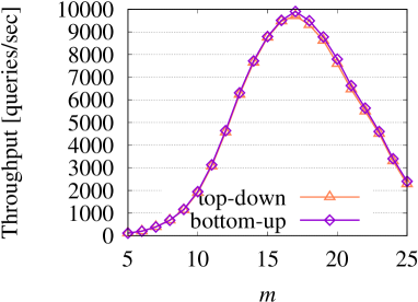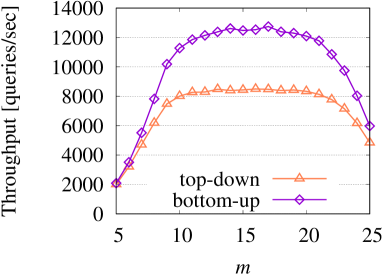
We compare the straightforward top-down approach for evaluating range queries on HINT^m that uses solely Lemma 1, against the bottom-up illustrated in Algorithm 3 which additionally employs Lemma 2. Figure 10 reports the throughput of each approach on BOOKS and TAXIS, while varying the number of levels $m$ in the index. Due to lack of space, we omit the results for WEBKIT and GREEND that follow exactly the same trend with BOOKS and TAXIS, respectively. We observe that the bottom-up approach significantly outperforms top-down for BOOKS while for TAXIS, this performance gap is very small. As expected, bottom-up performs at its best for inputs that contain long intervals which are indexed on high levels of index, i.e., the intervals in BOOKS. In contrast, the intervals in TAXIS are very short and so, indexed at the bottom level of HINT^m, while the majority of the partitions at the higher levels are empty. As a result, top-down conducts no comparisons at higher levels. For the rest of our tests, HINT^m uses the bottom-up approach (i.e., Algorithm 3).

5.2.2. Subdivisions and space decomposition

BOOKS	TAXIS

Figure 11. Optimizing HINT^m: subdivisions and space decomposition

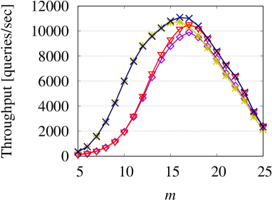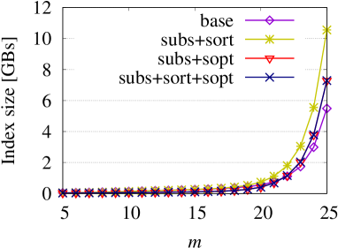
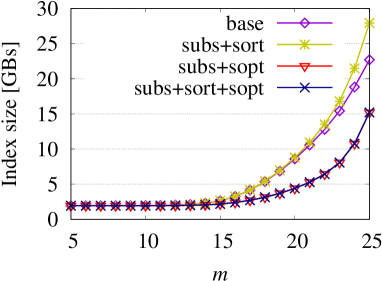
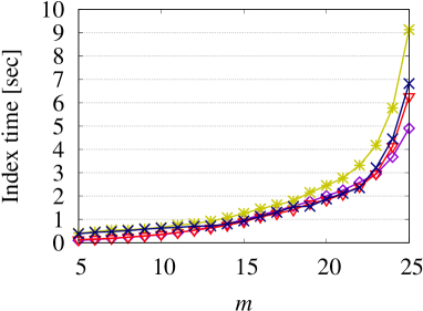
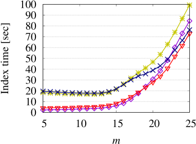
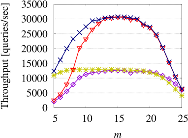
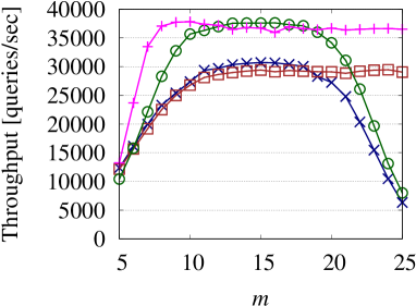
We next evaluate the subdivisions and space decomposition optimizations described in Section 4.1 for HINT^m. Note that these techniques are not applicable to our comparison-free HINT as the index stores only interval ids. Figure 11 shows the effect of the optimizations on BOOKS and TAXIS, for different values of $m$; similar trends were observed in WEBKIT and GREEND, respectively. The plots include (1) a base version of HINT^m, which employs none of the proposed optimizations, (2) subs+sort+sopt, with all optimizations activated, (3) subs+sort, which only sorts the subdivisions (Section 4.1.1) and (iv) subs+sopt, which uses only the storage optimization (Section 4.1.2). We observe that the subs+sort+sopt version of HINT^m is superior to all three other versions, on all tests. Essentially, the index benefits from the sub+sort setting only when $m$ is small, i.e., below 15, at the expense of increasing the index time compared to base. In this case, the partitions contain a large number of intervals and therefore, using binary search or scanning until the first interval that does not overlap the query range, will save on the conducted comparisons. On the other hand, the subs+sopt optimization significantly reduces the space requirements of the index. As a result, the version incurs a higher cache hit ratio and so, a higher throughput compared to base is achieved, especially for large values of $m$, i.e., higher than 10. The subs+sort+sopt version manages to combine the benefits of both subs+sort and subs+sopt versions, i.e., high throughput in all cases, with low space requirements. The effect in the performance is more obvious in BOOKS because of the long intervals and the high replication ratio. In view of these results, HINT^m employs all optimizations from Section 4.1 for the rest of our experiments.

5.2.3. Handling data skewness & sparsity and reducing cache misses

Table 6. Optimizing HINT: impact of the skewness & sparsity optimization (Section 4.2), default parameters

dataset	throughput [queries/sec]		index size [MBs]
	original	optimized	original	optimized
BOOKS	12098	36173	3282	273
WEBKIT	947	39000	49439	337
TAXIS	2931	31027	10093	7733
GREEND	648	47038	57667	10131

Table 6 tests the effect of the handling data skewness & sparsity optimization (Section 4.2) on the comparison-free version of HINT (Section 3.1). Observe that the optimization has a great effect on both the throughput and the size of the index in all four real datasets, because empty partitions are effectively excluded from query evaluation and from the indexing process.

BOOKS	TAXIS

Figure 12. Optimizing HINT^m: impact of handling skewness & sparsity and reducing cache misses optimizations

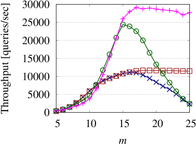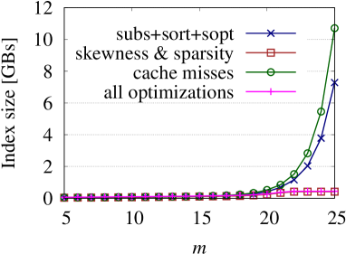
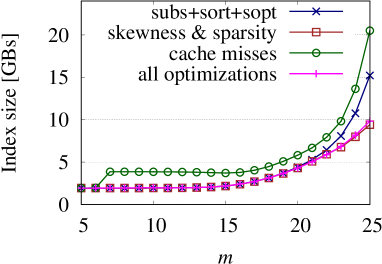
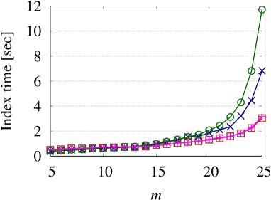
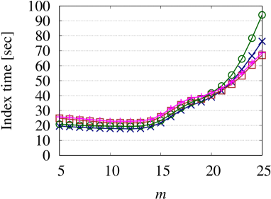
Figure 12 shows the effect of either or both of the data skewness & sparsity (Section 4.2) and the cache misses optimizations (Section 4.3) on the performance of HINT^m for different values of $m$. In all cases, the version of HINT^m which uses both optimizations is superior to all other versions. As expected, the skewness & sparsity optimization helps to reduce the space requirements of the index when $m$ is large, because there are many empty partitions in this case at the bottom levels of the index. At the same time, the cache misses optimization helps in reducing the number of cache misses in all cases where no comparisons are needed. Overall, the optimized version of $HINT^{m}$ converges to its best performance at a relatively small value of $m$, where the space requirements of the index are relatively low, especially on the BOOKS and WEBKIT datasets which contain long intervals. For the rest of our experiments, HINT^m employs both optimizations and HINT the data skewness & sparsity optimization.

5.2.4. Discussion

Table 7. Statistics and parameter setting

index	parameter	BOOKS	WEBKIT	TAXIS	GREEND
Period	# levels	4	4	7	8
	# coarse partitions	100	100	100	100
Timeline	# checkpoints	6000	6000	8000	8000
1D-grid	# partitions	500	300	4000	30000
HINTm	$m_{opt}$ (model)	9	9	16	16
	$m_{opt}$ (exps)	$10$	$12$	$17$	$17$
	rep. factor $k$ (model)	$6.09$	$8.98$	$1.98$	$1$
	rep. factor $k$ (exps)	$5.13$	$6.07$	$2.14$	$1.0013$
	avg. comp. part.	$3.226$	$3.538$	$3.856$	$2.937$

Table 7 reports the best values for parameter $m$ of HINT^m, denoted by $m_{opt}$. For each real dataset, we show (1) $m_{opt}$ (model), estimated by our model in Section 3.3 as the smallest $m$ value for which the index converges within 3% to its lowest estimated cost, and (2) $m_{opt}$ (exps), which brings the highest throughput in our tests. Overall, our model estimates a value of $m_{opt}$ which is very close to the experimentally best value of $m$. Despite a larger gap for WEBKIT, the measured throughput for the estimated $m_{opt}=9$ is only 5% lower than the best observed throughput. Further, the table shows the replication factor $k$ of the index, i.e., the average number of partitions in which each interval is stored, as predicted by our space complexity analysis (see Theorem 4) and as measured experimentally. As expected, the replication factor is high on BOOKS, WEBKIT due to the large number of long intervals, and low on TAXIS, GREEND where the intervals are very short and stored at the bottom levels. Although our analysis uses simple statistics, the predictions are quite accurate. Finally, the last line Table 7 (avg. comp. part.) shows the average number of HINT^m partitions for which comparisons were applied. Consistently to our analysis in Section 3.2.3, all numbers are below 4, which means that the performance of HINT^m is very close to the performance of the comparison-free, but space-demanding HINT.

Table 8. Comparing index size [MBs]

index	BOOKS	WEBKIT	TAXIS	GREEND
Interval tree	97	115	3125	2241
Period	210	217	2278	1262
Timeline	4916	5671	4203	2525
1D-grid	949	604	2165	1264
HINT	273	337	7733	10131
HINTm	81	98	2039	1278

Table 9. Comparing index time [sec]

index	BOOKS	WEBKIT	TAXIS	GREEND
Interval tree	0.249647	0.333642	47.1913	26.8279
Period	1.14919	1.35353	76.9302	46.3992
Timeline	12.665271	19.242939	40.376573	15.962221
1D-grid	1.26315	0.952408	4.02325	2.23768
HINT	1.70093	11.7671	49.589	36.5143
HINTm	0.725174	0.525927	22.787983	8.577486

5.3. Index performance comparison

Interval tree     Period index     Timeline index     1D-grid     HINT     HINT^m BOOKS WEBKIT TAXIS GREEND

Figure 13. Comparing throughputs, real datasets

Figure 14. Comparing throughputs, synthetic datasets

We next compare the optimized versions of HINT and HINT^m against the previous work competitors. We start with our tests on the real datasets. For HINT^m, we set $m$ to the best value on each dataset, according to Table 7. Similarly, we set the number of partitions for 1D-grid, the number of checkpoints for the timeline index, and the number of levels and number of coarse partitions for the period index (see Table 7). Table 8 shows the sizes of each index in memory and Table 9 shows the construction cost of each index, for the default query extent 0.1%. Regarding space, HINT^m along with the interval tree and the period index have the lowest requirements on datasets with long intervals (BOOKS and WEBKIT) and very similar to 1D-grid in the rest. In TAXIS and GREEND where the intervals are indexed mainly at the bottom level, the space requirements of HINT^m are significantly lower than our comparison-free HINT due to limiting the number of levels. When compared to the raw data (see Table 4), HINT^m is 2 to 3 times bigger for BOOKS and WEBKIT (which contain many long intervals), and 1 time bigger for GREEND and TAXIS. These ratios are smaller than the replication ratios $k$ reported in Table 7, due to our storage optimization (cf. Section 4.1.2). Due to its simplicity, 1D-grid has the lowest index time across all datasets. Nevertheless, HINT^m is the runner up in most of the cases, especially for the biggest inputs, i.e., TAXIS and GREEND, while in BOOKS and WEBKIT, its index time is very close to the interval tree.

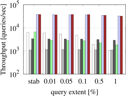
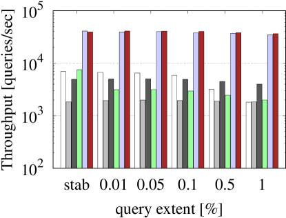
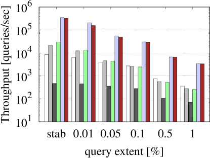
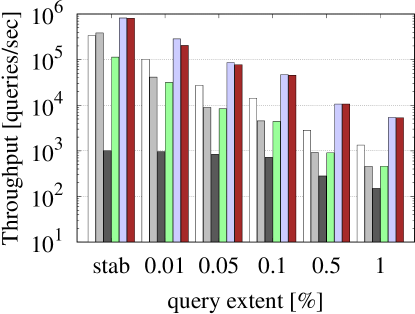
Figure 13 compares the query throughputs of all indices on queries of various extents (as a percentage of the domain size). The first set of bars in each plot corresponds to stabbing queries, i.e., range queries of 0 extent. We observe that HINT and HINT^m outperform the competition by almost one order of magnitude, across the board. In fact, only on GREEND the performance for one of the competitors, i.e., 1D-grid, comes close to the performance of our hierarchical indexing. Due to the extremely short intervals in GREEND (see Table 4) the vast majority of the results are collected from the bottom level of HINT/HINT^m, which essentially resembles the evaluation process in 1D-grid. Nevertheless, our indices are even in this case faster as they require no duplicate elimination.

HINT^m is the best index overall, as it achieves the performance of HINT, requiring less space, confirming the findings of our analysis in Section 3.2.3. As shown in Table 8, HINT always has higher space requirements than HINT^m; even up to an order of magnitude higher in case of GREEND. What is more, since HINT^m offers the option to control the occupied space in memory by appropriately setting the $m$ parameter, it can handle scenarios with space limitations. HINT is marginally better than HINT^m only on datasets with short intervals (TAXIS and GREEND) and only for selective queries. In these cases, the intervals are stored at the lowest levels of the hierarchy where HINT^m typically needs to conduct comparisons to identify results, but HINT applies comparison-free retrieval.

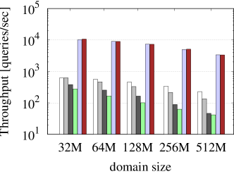
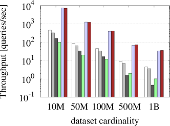
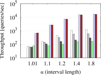
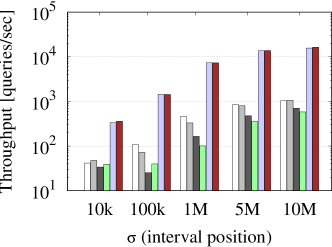
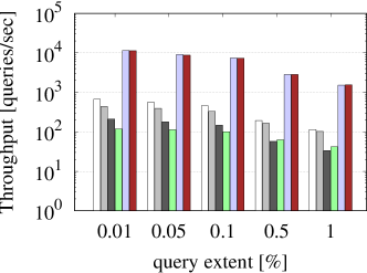
The next set of tests are on synthetic datasets. In each test, we fix all but one parameters (domain size, cardinality, $\alpha$, $\sigma$, query extent) to their default values and varied one (see Table 5). The value of $m$ for HINT^m, the number of partitions for 1D-grid, the number of checkpoints for the timeline index and the number of levels/coarse partitions for the period index are set to their best values on each dataset. The results, shown in Figure 14, follow a similar trend to the tests on the real datasets. HINT and HINT^m are always significantly faster than the competition, . Different to the real datasets, 1D-grid is steadily outperformed by the other three competitors. Intuitively, the uniform partitioning of the domain in 1D-grid cannot cope with the skewness of the synthetic datasets. As expected the domain size, the dataset cardinality and the query extent have a negative impact on the performance of all indices. Essentially, increasing the domain size under a fixed query extent, affects the performance similar to increasing the query extent, i.e., the queries become longer and less selective, including more results. Further, the querying cost grows linearly with the dataset size since the number of query results are proportional to it. HINT^m occupies around 8% more space than the raw data, because the replication factor $k$ is close to 1. In contrast, as $\alpha$ grows, the intervals become shorter, so the query performance improves. Similarly, when increasing $\sigma$ the intervals are more widespread, meaning that the queries are expected to retrieve fewer results, and the query cost drops accordingly.

Table 10. Throughput [operations/sec] and total cost [sec]

BOOKS
operation Interval tree Period index 1D-grid _subs+soptHINT^m HINT^m queries 1,258 3,088 3,739 14,390 40,311 insertions 5,841 519,904 411,540 2,405,228 3,680,457 deletions 1,142 765 165 2,201 5,928 total cost 9.63 4.52 8.68 1.14 0.41
TAXIS
operation Interval tree Period index 1D-grid _subs+soptHINT^m HINT^m queries 2,619 2,695 2,572 8,774 28,596 insertions 61,923 1,026,423 8,347,273 4,407,743 6,745,622 deletions 14,318 21,293 16,236 71,122 90,460 total cost 3.93 3.76 3.95 1.15 0.36

5.4. Updates

Finally, we test the efficiency of HINT^m in updates using both the update-friendly version of HINT^m (Section 3.4), denoted by _subs+soptHINT^m, and the hybrid setting for the fully-optimized index from Section 4.4, denoted as HINT^m. We index offline the first 90% of the intervals for each real dataset in batch and then execute a mixed workload with 10K range queries of 0.1% extent, 5K insertions of new intervals (randomly selected from the remaining 10% of the dataset) and 1K random deletions. Table 10 reports our findings for BOOKS and TAXIS; the results for WEBKIT and GREEND follow the same trend. Note that we excluded Timeline since the index is designed for temporal (versioned) data where updates only happen as new events are appended at the end of the event list, and the comparison-free HINT, for which our tests have already shown a similar performance to HINT^m with higher indexing/storing costs. Also, all indices handle deletions with “tombstones”. We observe that both versions of HINT^m outperform the competition by a wide margin. An exception arises on TAXIS, as the short intervals are inserted in only one partition in 1D-grid. The interval tree has in fact several orders of magnitude slower updates due to the extra cost of maintaining the partitions in the tree sorted at all time. Overall, we also observe that the hybrid HINT^m setting is the most efficient index as the smaller delta _subs+soptHINT^m handles insertions faster than the 90% pre-filled _subs+soptHINT^m.

6. Conclusions and Future Work

We proposed a hierarchical index (HINT) for intervals, which has low space complexity and minimizes the number of data accesses and comparisons during query evaluation. Our experiments on real and synthetic datasets shows that HINT outperforms previous work by one order of magnitude in a wide variety of interval data and query distributions. There are several directions for future work. First, we plan to study the performance of HINT on selection queries, based on Allen’s relationships (Allen, 1981) between intervals and on complex event processing in data streams, based on interval operators (Awad et al., 2022). Second, we plan to investigate extensions of HINT for supporting queries that combine temporal selections and selections on additional object attributes or the duration of intervals (Behrend et al., 2019). Third, we plan to investigate effective parallelization techniques, taking advantage of the fact that HINT partitions are independent.

References

- (1)
- Allen (1981) James F. Allen. 1981. An Interval-Based Representation of Temporal Knowledge. In IJCAI. 221–226.
- Awad et al. (2022) Ahmed Awad, Riccardo Tommasini, Samuele Langhi, Mahmoud Kamel, Emanuele Della Valle, and Sherif Sakr. 2022. D2IA: User-defined interval analytics on distributed streams. Information Systems 104 (2022), 101679.
- Becker et al. (1996) Bruno Becker, Stephan Gschwind, Thomas Ohler, Bernhard Seeger, and Peter Widmayer. 1996. An Asymptotically Optimal Multiversion B-Tree. VLDB J. 5, 4 (1996), 264–275.
- Behrend et al. (2019) Andreas Behrend, Anton Dignös, Johann Gamper, Philip Schmiegelt, Hannes Voigt, Matthias Rottmann, and Karsten Kahl. 2019. Period Index: A Learned 2D Hash Index for Range and Duration Queries. In SSTD. 100–109.
- Böhlen et al. (2017) Michael H. Böhlen, Anton Dignös, Johann Gamper, and Christian S. Jensen. 2017. Temporal Data Management - An Overview. In eBISS. 51–83.
- Bouros et al. (2020) Panagiotis Bouros, Konstantinos Lampropoulos, Dimitrios Tsitsigkos, Nikos Mamoulis, and Manolis Terrovitis. 2020. Band Joins for Interval Data. In EDBT. 443–446.
- Bouros and Mamoulis (2017) Panagiotis Bouros and Nikos Mamoulis. 2017. A Forward Scan based Plane Sweep Algorithm for Parallel Interval Joins. Proc. VLDB Endow. 10, 11 (2017), 1346–1357.
- Bouros and Mamoulis (2018) Panagiotis Bouros and Nikos Mamoulis. 2018. Interval Count Semi-Joins. In EDBT. 425–428.
- Bouros et al. (2021) Panagiotis Bouros, Nikos Mamoulis, Dimitrios Tsitsigkos, and Manolis Terrovitis. 2021. In-Memory Interval Joins. VLDB J. 30, 4 (2021).
- Cafagna and Böhlen (2017) Francesco Cafagna and Michael H. Böhlen. 2017. Disjoint interval partitioning. VLDB J. 26, 3 (2017), 447–466.
- Chekol et al. (2019) Melisachew Wudage Chekol, Giuseppe Pirrò, and Heiner Stuckenschmidt. 2019. Fast Interval Joins for Temporal SPARQL Queries. In ACM WWW. 1148–1154.
- Dalvi and Suciu (2004) Nilesh N. Dalvi and Dan Suciu. 2004. Efficient Query Evaluation on Probabilistic Databases. In VLDB. 864–875.
- de Berg et al. (2008) Mark de Berg, Otfried Cheong, Marc J. van Kreveld, and Mark H. Overmars. 2008. Computational geometry: algorithms and applications, 3rd Edition. Springer.
- Dignös et al. (2014) Anton Dignös, Michael H. Böhlen, and Johann Gamper. 2014. Overlap interval partition join. In ACM SIGMOD. 1459–1470.
- Dittrich and Seeger (2000) Jens-Peter Dittrich and Bernhard Seeger. 2000. Data Redundancy and Duplicate Detection in Spatial Join Processing. In IEEE ICDE. 535–546.
- Edelsbrunner (1980) Herbert Edelsbrunner. 1980. Dynamic Rectangle Intersection Searching. Technical Report 47. Institute for Information Processing, Technical University of Graz, Austria.
- Ferragina and Vinciguerra (2020) Paolo Ferragina and Giorgio Vinciguerra. 2020. The PGM-index: a fully-dynamic compressed learned index with provable worst-case bounds. Proc. VLDB Endow. 13, 8 (2020), 1162–1175.
- Garrison ([n.d.]) Erik Garrison. [n.d.]. A minimal C++ interval tree implementation. https://github.com/ekg/intervaltree.
- Kaufmann et al. (2013) Martin Kaufmann, Amin Amiri Manjili, Panagiotis Vagenas, Peter M. Fischer, Donald Kossmann, Franz Färber, and Norman May. 2013. Timeline index: a unified data structure for processing queries on temporal data in SAP HANA. In ACM SIGMOD. 1173–1184.
- Kline and Snodgrass (1995) Nick Kline and Richard T. Snodgrass. 1995. Computing Temporal Aggregates. In IEEE ICDE. 222–231.
- Kriegel et al. (2000) Hans-Peter Kriegel, Marco Pötke, and Thomas Seidl. 2000. Managing Intervals Efficiently in Object-Relational Databases. In VLDB. 407–418.
- Lomet (1975) David B. Lomet. 1975. Scheme for Invalidating References to Freed Storage. IBM J. Res. Dev. 19, 1 (1975), 26–35.
- Lomet et al. (2008) David B. Lomet, Mingsheng Hong, Rimma V. Nehme, and Rui Zhang. 2008. Transaction time indexing with version compression. Proc. VLDB Endow. 1, 1 (2008), 870–881.
- Min et al. (2003) Jun-Ki Min, Myung-Jae Park, and Chin-Wan Chung. 2003. XPRESS: A Queriable Compression for XML Data. In ACM SIGMOD. 122–133.
- Monacchi et al. (2014) Andrea Monacchi, Dominik Egarter, Wilfried Elmenreich, Salvatore D’Alessandro, and Andrea M. Tonello. 2014. GREEND: An energy consumption dataset of households in Italy and Austria. In SmartGridComm. 511–516.
- Moon et al. (2003) Bongki Moon, Inés Fernando Vega López, and Vijaykumar Immanuel. 2003. Efficient Algorithms for Large-Scale Temporal Aggregation. IEEE TKDE 15, 3 (2003), 744–759.
- Overmars (1983) Mark H. Overmars. 1983. The Design of Dynamic Data Structures. Lecture Notes in Computer Science, Vol. 156. Springer.
- Pagel et al. (1993) Bernd-Uwe Pagel, Hans-Werner Six, Heinrich Toben, and Peter Widmayer. 1993. Towards an Analysis of Range Query Performance in Spatial Data Structures. In ACM PODS. 214–221.
- Piatov and Helmer (2017) Danila Piatov and Sven Helmer. 2017. Sweeping-Based Temporal Aggregation. In SSTD. 125–144.
- Piatov et al. (2016) Danila Piatov, Sven Helmer, and Anton Dignös. 2016. An interval join optimized for modern hardware. In IEEE ICDE. 1098–1109.
- Piatov et al. (2021) Danila Piatov, Sven Helmer, Anton Dignös, and Fabio Persia. 2021. Cache-efficient sweeping-based interval joins for extended Allen relation predicates. VLDB J. 30, 3 (2021), 379–402.
- Salzberg and Tsotras (1999) Betty Salzberg and Vassilis J. Tsotras. 1999. Comparison of Access Methods for Time-Evolving Data. ACM Comput. Surv. 31, 2 (1999), 158–221.
- Samarati and Sweeney (1998) Pierangela Samarati and Latanya Sweeney. 1998. Generalizing Data to Provide Anonymity when Disclosing Information (Abstract). In ACM PODS. 188.
- Snodgrass and Ahn (1986) Richard T. Snodgrass and Ilsoo Ahn. 1986. Temporal Databases. Computer 19, 9 (1986), 35–42.
- Zhu et al. (2019) Kaijie Zhu, George H. L. Fletcher, Nikolay Yakovets, Odysseas Papapetrou, and Yuqing Wu. 2019. Scalable temporal clique enumeration. In SSTD. 120–129.