A novel approach to optimize the regularization and evaluation of dynamical models using a model selection framework
Abstract
Orbit superposition models are a non-parametric dynamical modelling technique to determine the mass of a galaxy’s central supermassive black hole (SMBH), its stars, or its dark-matter halo. One of the main problems is how to decide which model out of a large pool of trial models based on different assumed mass distributions represents the true structure of an observed galaxy best. We show that the traditional approach to judge models solely by their goodness-of-fit can lead to substantial biases in estimated galaxy properties caused by varying model flexibilities. We demonstrate how the flexibility of the models can be estimated using bootstrap iterations and present a model selection framework that removes these biases by taking the variable flexibility into account in the model evaluation. We extend the model selection approach to optimize the degree of regularisation directly from the data. Altogether, this leads to a significant improvement of the constraining power of the modeling technique. We show with simulations that one can reconstruct the mass, anisotropy and viewing angle of an axisymmetric galaxy with a few percent accuracy from realistic observational data with fully resolved line-of-sight velocity distributions (LOSVDs). In a first application, we reproduce a photometric estimate of the inclination of the disk galaxy NGC 3368 to within 5 degree accuracy from kinematic data that cover only a few sphere-of-influence radii around the galaxy’s SMBH. This demonstrates the constraining power that can be achieved with orbit models based on fully resolved LOSVDs and a model selection framework.
keywords:
galaxies: structure – galaxies: kinematics and dynamics – galaxies: individual (NGC 3368) – methods: statistical.1 Introduction
Revealing the internal structure of external galaxies is a challenging, yet essential task for a broader understanding of galaxy evolution. Since observations of external galaxies are limited to the projected kinematics and the surface brightness of the luminous galaxy components the common approach is to establish dynamical models of an observed galaxy and to compare their projections to the corresponding observations. A collisionless galaxy component, such as the ensemble of its stars, follows the collisonless Boltzmann equation and can be fully characterized by its phase-space distribution function. Therefore a dynamical model can, at least in principal, describe such a system of stars if it can sufficiently emulate the real distribution function. If a galaxy could not be assumed to be in equilibrium, dealing with all the freedom in the distribution function during the modelling process would be hopeless. However, in equilibrium the Jeans Theorem can be invoked (e.g. Binney & Tremaine, 2008) and the distribution function has a relatively simple structure which can be expressed as a function of the integrals of motion meaning it takes the form of an orbit superposition.
Even though stellar systems with a high degree of symmetry can sometimes be modelled well using analytic distribution functions, a more universal approach to dynamical modelling is generally required to deal with the full range of compatible distribution functions. Schwarzschild modelling is an efficient numerical approach based on the superposition of stellar orbits to construct such dynamical models. In its initial version, established by Schwarzschild (1979), such orbit models were designed to replicate a given triaxial density distribution in a self-consistent manner. In the subsequent decades the Schwarzschild technique was extended to include the fitting of kinematic observations (e.g. Levison & Richstone, 1985; Rix et al., 1997; Cretton et al., 1999; Thomas et al., 2004; van den Bosch et al., 2008), making it possible to constrain the distribution function of an observed galaxy more tightly and enabling the estimation of intrinsic properties of stellar systems such as black hole mass (e.g. van der Marel et al., 1998; Gebhardt et al., 2000; Cappellari et al., 2002; Gebhardt et al., 2003; Rusli et al., 2013), mass-to-light ratios (e.g. Thomas et al., 2005; Cappellari et al., 2006; Thomas et al., 2011), dark matter halos (e.g. Thomas et al., 2005, 2007b, 2009b; Rusli et al., 2013; Leung et al., 2018), the velocity dispersion anisotropy and orbital structure (e.g. van de Ven et al., 2008; Thomas et al., 2009a; Thomas et al., 2014; Kowalczyk et al., 2017), and the intrinsic shape of the stellar distribution (e.g. Jin et al., 2020).
Several different implementations of the Schwarzschild Method with varying degrees of symmetry have been described (e.g. Rix et al., 1997; Cretton et al., 1999; Siopis & Kandrup, 2000; Häfner et al., 2000; Gebhardt et al., 2000, 2003; Valluri et al., 2004; Thomas et al., 2004; van den Bosch et al., 2008; Vasiliev & Athanassoula, 2015; Vasiliev & Valluri, 2020; Neureiter et al., 2021), but the main steps of the method are rather general. Very briefly: If an assumed gravitational potential is given, one needs to compute tens of thousands of representative orbits in the available phase space. These orbits are combined to a galaxy model, where each orbit can carry an adjustable number of stars. These so-called orbital weights (or orbital occupation numbers) together with each orbits intrinsic and projected properties then determine the dynamical model. Through optimization of the orbital weights, the model can be adapted to the observations. In this sense, the orbital weights are the variables of the model. While different algorithms are used for this weight optimization, they are all tied to a -minimisation framework.
With the rise of integral-field spectrographs in the last decade, the amount of kinematic data that can be used to constrain these models has increased significantly. While many early studies had to rely on line-of-sight velocity distributions (LOSVDs) that were parameterized by Gauss-Hermite series expansions (Gerhard, 1993; van der Marel & Franx, 1993) up to fourth order (often along a 1d slit (Bender et al., 1994), it is now often possible to reliably obtain higher Gauss-Hermite moments (e.g. Krajnović et al., 2009; Liepold et al., 2020) or measure the fully resolved, non-parametric LOSVDs over the 2d sky area occupied by the galaxy (Mehrgan et al., 2019). The number of measured data points per galaxy has thus increased from a few dozen to several thousands. Still, one of the characteristics of the Schwarzschild Method is that one is usually faced with a situation where the number of free model parameters is significantly larger than the number of observational data points, mainly because the number of orbits is typically very large and each orbit is associated with a free orbital weight parameter. For simple, linear models this would imply a negative number of degrees of freedom of the resulting distribution (Press et al., 1992) and the solution of the -minimization is non-unique (cf. Valluri et al., 2004; Magorrian, 2006; Neureiter et al., 2021). Under the assumption that a model is generally detailed enough to deal with all the structure in the data, one would consequently expect that every data set is perfectly fitted due to the models comparatively huge number of free parameters, resulting in a . In practice, this does not happen for two reasons. Firstly, data with a realistic amount of noise can not be fitted perfectly when the orbital weights are constrained to be non-negative (see Magorrian 2006 for a discussion). Secondly, a perfect fit is suppressed when a regularisation term is applied in the weight optimisation, e.g. via the commonly used maximum penalized likelihood or maximum entropy approaches. The smoothing induced by such a regularization term allows to discard physically implausible solutions and prevents overfitting by effectively reducing the flexibility of the dynamical model. Despite the differences in the individual implementations of regularization, the result is always the same: The of the regularized model is significantly larger than zero even though the model’s parameters typically outnumber the data points. This suggests that the effective number of free parameters is smaller than the nominal number of variables in the model, implying a reduction in the model’s flexibility (i.e. its ability to fit noisy data). Beyond the regularization another core aspect in reducing the flexibility of Schwarzschild models is the prior constraint on the orbital weights to be non-negative to avoid negative phase-spaces densities in the model.
The reduction of model flexibility is a generic property of regularized models, of models with prior constraints imposed on their free parameters, or in general of non-linear models (cf. Andrae et al., 2010). As a consequence, because the effective number of parameters is an unknown, the interpretation of the absolute value of becomes less obvious. This is particularly important, because in most Schwarzschild applications, the primary interest is not in the distribution of the orbital weights. Instead, one aims to determine the mass composition of a galaxy, which requires the comparison of a number of Schwarzschild models that were obtained with different trial gravitational potentials. Traditionally this comparison is done by evaluating the values inherited from the orbital weight optimization of each trial model. Given the fact that these values depend on the model flexibility (or its effective number of free parameters) it may be important to take this into account in the evaluation process.
The goal of this paper is threefold. Firstly, we provide a method to estimate the flexibility of Schwarzschild Models, or the effective number of free parameters respectively, that can robustly deal with all the smoothing constraints, positivity constraints and non-linearities of the models. Secondly, we demonstrate that varying model flexibilities lead to biased surfaces when evaluating orbit models obtained using different mass distributions, viewing angles or assumed regularisation powers. Thirdly, we provide a model selection framework that allows to overcome these biases that can arise in the simple comparison framework. The new framework not only improves the constraining power of Schwarzschild models significantly, but also enables a new data-driven approach to optimize the amount of regularization. All these considerations can probably be generalised to other non-linear, non-parametric, non-dynamical models that involve regularisation or prior constraints.
As the main application example, we investigate the reconstruction of the viewing angle (or equivalently the intrinsic flattening) under which an axisymmetric galaxy is observed. The question whether it is feasible to constrain the inclination/intrinsic shape via dynamical modelling is as of yet a point of contention. In early works Verolme et al. (2002) argue that they constrained the inclination of M32 to using axisymmetric, three-integral, Schwarzschild models. However, follow-up results of Krajnović et al. (2005), who tried to recover the inclination of semi-analytic galaxy models with axisymmetric models, suggest that different inclinations are degenerate even under ideal conditions. Cappellari et al. (2006) confirmed these results for a large sample of early-type galaxies in so far as they state that Schwarzschild models with a wide range of inclinations are able to fit the observed kinematics well within the errors. Onken et al. (2007) modelled the bulge of the Seyfert 1 galaxy NGC 4151 edge-on and with an inclination obtained from the observed ellipticity of the large-scale disk, with the result that the edge-on model provides better fits to the kinematic constraints than the model, suggesting either that the bulge is not aligned with the disk or that the inclination recovery using dynamical modelling is biased. Similarly, Thomas et al. (2007b) found that a surprising amount of the 17 early-type galaxies they dynamically modelled with axisymmetric three-integral models are fitted best when the orbit model is viewed edge-on and they argue there may be a small inclination bias favoring edge-on Schwarzschild models. In this paper we will demonstrate that the assumed inclination strongly affects the flexibilty of orbit models which could explain the observed edge-on preference of previous studies. We will show that the inclination of axisymmetric galaxies can be well constrained from typical observational data with the new model selection framework as it considers the model flexibility in the evaluation of the fitted models.
The paper is organized as follows: In section 2 we outline our motivation for using a model selection approach in the evaluation of Schwarzschild models in detail. In section 3 we lay out two bootstrap methods which facilitate the quantification of a model’s intrinsic flexibility. A discussion of an evaluation approach based on model selection techniques follows in section 4. We then test the model selection with respect to the inclination reconstruction on a number of simulated galaxies in section 5. In section 6 we extend the analysis to mass parameters. Section 7 further refines our approach by including the regularization power. Equipped with all these insights we model the disk galaxy NGC 3368 in section 8 with our refined model selection framework and set it into contrast to the prevalent -minimization. Sec. 9 discusses general aspects related to modelling degeneracies and the inclination recovery. The paper concludes with a summary in section 10.
2 Motivating a model selection approach to the Schwarzschild technique
As mentioned in the Introduction above, we want to demonstrate the power of the model selection framework using the example of Schwarzschild orbit superposition models. The main reasons for picking up Schwarzschild models are: (i) This technique is very general and allows to model any kind of galaxy without apriori assumptions upon the orbital structure; (ii) The method is observationally not restricted to moments of the velocity distribution of the stars but instead can deal with the full information contained in the line-of-sight velocity distributions (e.g. Thomas et al., 2004; Mehrgan et al., 2019; Vasiliev & Valluri, 2020; Neureiter et al., 2021). The specific implementation of the Schwarzschild Method that we consider in this paper assumes axially symmetric galaxies and is described in detail in Thomas et al. (2004).
In Schwarzschild models, one first specifies a trial mass distribution and viewing angle via parameters like the stellar mass-to-light ratio , black-hole mass , dark-halo parameters and inclination . Then one calculates an orbit library with thousands of orbits whose projected properties form the building blocks of the superposition model. By computing the best-fitting orbital weights one can assess how well the trial mass distribution allows to explain the observational data. A systematic search through the space of trial mass models then leads to the identification of a best-fit mass distribution for each galaxy. This is only a very brief sketch of the method (we provide a more detailed description in App. A and Sec. 2.1) but it already demonstrates one important aspect: the fact that one first needs to specify a set of mass parameters (and the inclination) before the orbit distribution can be determined will turn out to be significant. As a consequence it is helpful to conceptually distinguish two distinct parameter layers that together define the properties of every Schwarzschild model: Minimization parameters (orbital weights ) and selection parameters (all other parameters, i.e. …). It is the latter parameters that require an evaluation using a model selection framework.
We present our reasoning for this distinction of parameter layers in Secs. 2.1 and 2.2. We also recapitulate our regularization approach to finding the optimum minimization parameters (i.e. orbital weights) in 2.2. The theoretically less interested reader may skip ahead to Sec. 2.3 where we show that a simple evaluation where all parameters are treated equally can lead to a bias, using the inclination as an example. As we will show throughout this paper, other selection parameters such as the stellar mass can also suffer from such a bias.
2.1 Selection vs. minimization parameters
It is tempting to consider the question of identifying the best-fit Schwarzschild model in terms of a huge minimisation, where all the parameters are treated equally as free parameters of a single ’global’ Schwarzschild model. This concerns mass parameters like and , viewing angles like the inclination and the orbital weights (cf. App. A). It is therefore common practice to assume that the best choice for is given by the trial set that resulted in the smallest without much concern of the role of orbital weights.
Using a sophisticated Bayesian framework Magorrian (2006) acknowledges that there often exist many possible combinations of orbital weights (or equivalently distribution functions) that are consistent with given observational data and an assumed trial potential. Magorrian (2006) argues that a more appropriate approach sums over all possible distribution functions for a given potential. This is achieved by marginalizing over the orbital weights and weighing the corresponding likelihoods by a suitable prior. Magorrian (2006) argues that this approach allows a more accurate calculation of the likelihood for a given potential, and that the odds of one set of trial parameters over another can be evaluated by the ratio of the likelihoods of the two potentials they generate.
The Bayesian framework of Magorrian (2006) does not specifically address the problem that the orbital weights are not independent parameters of a single, global Schwarzschild model. Instead, the orbital weights function as (linear) coefficients for the fundamental building blocks of the model: the projected properties of the orbits which are different for each trial potential and, thus, need to be recalculated from scratch for each trial potential (cf. Appendix A). In other words, the subjects to which the orbital weights refer to, depend on the choice of the parameters which have to be specified to generate the orbits. This means there is no straight-forward way to define a single model with a common parameter space as the basis for the comparison of values obtained for different sets of trial parameters like or . Instead one actually compares the goodness-of-fit of distinct statistical models, each with its own individual space of orbital weights .
On a more fundamental level, the Schwarzschild technique is an exact method to find phase-space distribution functions that obey the Collisionless Boltzmann equation:
| (1) |
(where is the gravitational potential and is the phase-space distribution function of the system under study). We can formulate the Schwarzschild technique by considering a partition of phase space into a huge number of small cells. The distribution function is represented by the large number of phase-space densities in each of these small local cells. The observables of the model, such as the binned LOSVDs of the model or its binned 3d luminosity density , can be derived from the by simple phase-space integrations, e.g. the amount of light in bin reads
| (2) |
where the integral goes over the whole velocity space and over the subset of the configuration space that represents bin (cf. App. A for the exact definitions and vector notation of and ). One could argue that these could be used as the fundamental parameters in a single, global Schwarzschild model.
In fact, when we do a minimization, we assume a statistical model for the data, specifically that each measurement was drawn from a Gaussian distribution. The width of this distribution is commonly assumed to be known and approximated by the observational error. Only the mean, which is given by has to be determined in the modelling process. Hence, our statistical model is completely determined when the are known, which is the case when the are specified. For this, we do not even need to assume a gravitational potential or mass model. And up to this point one could indeed formulate a single, global dynamical phase-space model with the being independent free parameters.
However, one issue with such a phase-space model is that arbitrary distributions of the are of little interest, because most of them will be physically unrealistic or even unphysical. Besides the constraint (positive phase-space density) another crucial requirement is given by the fact that we are only interested in equilibrium solutions, or more specifically, in solutions that represent a stationary state. The Jeans Theorem then implies that two phase-space cells and that happen to be located along the same orbit necessarily have to carry the same . It is this constraint – that the phase-space density is constant along orbits – which gives equilibrium solutions of Eq. (1) the form of orbit superpositions and allows us to use orbits as building blocks for the models. In practice, thus, the Jeans Theorem introduces many, many nonlinear equality constraint equations for our statistical model if we formulate it on the fundamental level of the . These equations require the assumption of a gravitational potential and will change as soon as the parameters of the assumed mass distribution (like etc) will change: the equilibrium distributions depend on the mass structure. Hence, the set of feasible points, i.e. the set of that fulfill the constraint equations will change as well. This shows that the selection parameters are not free parameters in the same sense as the because they are required to define the constraint equations that regulate the domain of the model. In fact, when these constraint equations change, one effectively deals with a different statistical model with a potentially different model complexity.
The above chain of arguments can be applied to any parameter that affects the gravitational potential and, thus, the stellar orbits, e.g. the stellar or the DM halo parameters. It also holds for the inclination , or more generally, for the viewing angles. One reason is that assuming different viewing angles changes the deprojection and with it the stellar contribution to the gravitational potential. Even if the latter is kept fixed, however, the (self-consistency) constraints imposed on the model’s stellar density do change (cf. App. A). This, in turn, means that the set of feasible points changes with the same consequences as discussed above.
Taking all this together it is clear that parameters like and the DM halo parameters on the one side and the orbital weights on the other, do not "operate" on the same level. It is conceptionally helpful to categorize them into two different parameter classes: selection parameters and minimization parameters. The selection parameters define a family of models . Each specific set of selection parameters defines a member of this family, i.e. a single statistical model for the measured LOSVDs. The free parameters of such a member model, i.e. the parameters to be minimised, are the orbital weights associated with the specific set of selection parameters. From one model to another the are assigned to different sets of orbits and they cannot be easily interchanged with each other across different models.
As illustrated above treating the problem of finding the optimum selection parameters as a selection of multiple distinct candidate models is a straight-forward approach, whereas a parameter estimation approach using of a single global Schwarzschild model is rather ambiguous due to the dependence of the orbital weights on the selection parameters. Furthermore the model selection framework is nothing but a generalization of the parameter estimation via which would simplify to the latter if the multiple (sub-)models would stem from a single, statistical model (cf. Sec. 4). Similarly, the generalization of the Bayesian framework introduced by Magorrian (2006) to a (Bayesian) model selection framework is straight forward and model selection criteria such as the Akaike criterion can be derived from it by choosing a suitable prior which penalizes flexibility (cf. Burnham et al., 2002).
2.2 Identifying the optimum minimization parameters
Finding the optimal set of minimization parameters (i.e. orbital weights ) for a given set of selection parameters is in principle a direct parameter estimation problem. The goal is to minimise
| (3) |
where is the number of spatially resolved bins and the number of velocity bins in a single spatial bin. However, in Schwarzschild models one is often faced with the problem that the free parameters (i.e. the number of orbits calculated for a given trial mass distribution) outnumber the observational constraints . The related optimisation problem is therefore underconstrained. In order to be able to decide on a set of unique and simultaneously prevent overfitting it is common practice to introduce regularization in the fitting process. We do this by maximizing the entropy-like term proposed by Richstone & Tremaine (1988):
| (4) |
where is a regularization parameter and S is the Boltzmann entropy defined by:
| (5) |
Here, is the phase-space volume of orbit such that is the phase-space density along the orbit. The entropy term in eq.( 4) guarantees that the optimisation problem has a unique solution for the orbital weights w (cf. the extensive discussion in Neureiter et al. 2021). The choice of equation 5 as the smoothing function is somewhat arbitrary though. The motivation behind maximising eq. (5) is that it yields and, hence, (in the absence of other constraints). In other words, it tends to smooth the corresponding physical phase-space distribution function rather than the distribution of the , which are only parameters. Neureiter et al. (2021) discuss how the more general form
| (6) |
can be used to explore the full range of all (possibly degenerate) solutions for a given set of kinematic observations.
The regularization parameter determines the smoothness of the model distribution function, meaning a small implies the entropy term in equation 4 dominates and the phase-space density is smooth, while a larger leads to a better fit but increases the possibility of overfitting. This raises the question which amount of regularization is optimal to represent the phase-space density of the observed galaxy. Using Monte-Carlo simulations of isotropic rotator models Thomas et al. (2005) describes an approach to estimate the optimum for NGC 4807. However, such simulations would be required for every newly modelled galaxy as the optimum depends on the obtained data and the underlying galaxy structure. In section 7 we will come back to this issue and provide a method to determine a more optimal amount of smoothing by treating as a selection parameter. In general, all the intrinsic parameters that control the behaviour of the models can be treated as selection parameters. Although we will not discuss it in full depth in this paper, another important selection parameter besides is the number of orbits used in the models.
In conclusion, the modelling process can be described using two fundamentally different parameter layers that together define the properties of an orbit model. For the primary parameter layer the modeller has to choose a set of selection parameters, including mass and library parameters, which define the fundamental building blocks of a Schwarzschild model. In contrast, the minimization parameters that form the second layer, i.e. the orbital weights, are estimated using a form of parameter estimation for the given observational constraints. In our case this parameter estimation is performed by maximizing the entropy-like quantity in equation 4. This estimation process of the minimization parameters is only concerned with finding a good set of orbital weights. In fact, it is only possible if all selection parameters required for the calculation of the orbits are fixed and established, i.e. if a specific model out of the family of all possible models has been selected. Consequently one has to construct multiple trial models, if the goal is to optimize the selection parameters. To this end one has to sample the selection parameter space, estimate the best set of for each of the resulting orbits (using eq. 4), and compare the properties of each model afterwards. Since these models consist of different building blocks they are fundamentally distinct and one has to establish a framework to evaluate which one of them results in the best approximation of the galaxy’s underlying structure.
As already stated above, the common approach to evaluate different models and with different selection parameters based on (cf. equation 3) is not optimal. We will show that judging models solely in terms of their goodness-of-fit can induce biases in the recovered selection parameters. The next section demonstrates such a case for a selection parameter that is very heavily impacted by this: The inclination of axisymmetric models.
2.3 Biases in selection parameters: The inclination as an example
We tested the Schwarzschild technique described in the previous section by applying it to a simulated spherical galaxy. For this purpose we created a number of mock LOSVDs obtained from an N-body model of an isotropic spherical galaxy (Hernquist, 1990). We sampled the sphere with particles and added Monte-Carlo noise to the corresponding LOSVDs. The underlying Hernquist density we used had a total mass , a mass-to-light ratio and an effective radius of kpc. The stellar kinematics of the N-body was projected to a grid of 80 angular and radial bins reaching out to approximately 2.3 effective radii. In total we simulated 10 independent observations of this spherical galaxy by adding random uncorrelated Gaussian noise with a standard deviation of two percent of the maximum LOSVD value in the respective spatial bin. Quantifying this noise in terms of the Gauss-Hermite coefficients (cf. van der Marel & Franx, 1993) this translates to an average error of and . The resulting Gauss-Hermite coefficients of one of these mocks are shown in Fig. 25 and 26 of the appendix. Without the Gaussian noise the N-body models follow the semi-analytic Gauss-Hermite profiles of (cf. Baes et al., 2005) very closely, which means that the odd Gauss-Hermite coefficients are zero everywhere, the velocity dispersion has a maximum at intermediate radii and is slightly negative but increases significantly for .
We modelled the spherical mocks with differently inclined, axisymmetric Schwarzschild models using the same spherical Hernquist density that was used to create the N-body in the first place. Thus, effectively we used the same orbit library for all models, yet the orbits were projected under different viewing angles. The resulting values as function of the inclination are shown in Fig. 1.
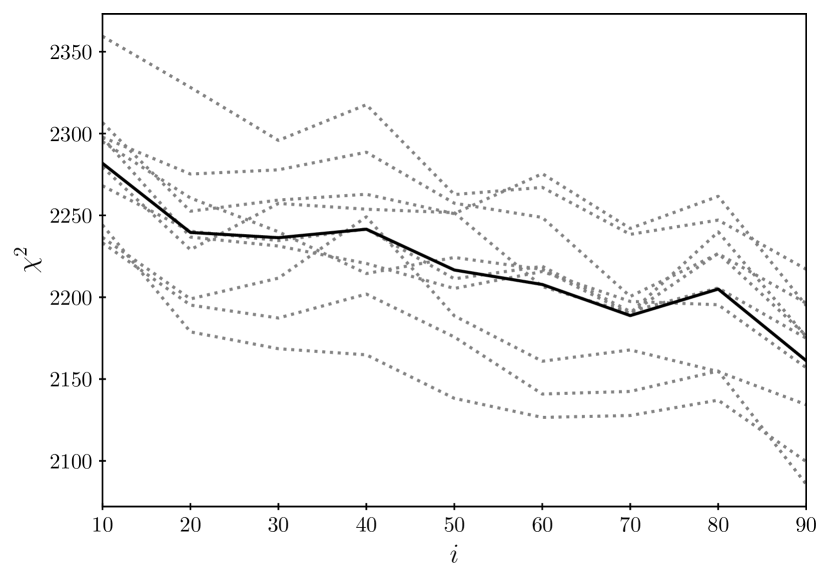
All 10 mocks exhibit a significant bias towards edge-on models, implying that the ability of an orbit model to fit data depends on the angle it is observed at. The reason for this behaviour is the axisymmetry of our Schwarzschild models: Every orbit in our model exists in a prograde and a retrograde version. In the case of an edge-on model the LOSVD of the prograde and retrograde version have opposite signs and are each a unique contribution to the model’s LOSVDs in equation 20. This is contrasted by a face-on model where the prograde and retrograde version are identical in projection, thus effectively reducing the number of unique base functions in equation 20. This weakens the flexibility of our model LOSVDs to fit the observations and consequently leads to a higher of face-on models when compared to their edge-on counterparts. Since this effect is intrinsic to the modelling technique, the edge-on bias will also be present when non-spherical galaxies are modelled, thus diminishing the possibility of successfully constraining the actual inclination of a galaxy. Therefore we should aim to quantify the variable model flexibility and use that to correct our results for the inclination constraints.
3 Model flexibility
In section 2 we showed that evaluating Schwarzschild models based on their can suffer from a bias if models with varying flexibility are compared. Therefore we introduce two methods in section 3.1 with the goal to estimate this flexibility, followed by an outline of three model selection approaches in section 4 which exploit this information to improve the constraining power of our models.
3.1 Estimating the model flexibility in Schwarzschild models
In statistical modelling a model’s general ability to fit data is quantified by its number of free parameters m, because every free parameter reduces the degrees of freedom of the distribution. This means if we assume uncorrelated Gaussian noise and quantify the deviations of N observed data points to a statistical model with m free parameters then the expectation value of the respective will be with variance . Therefore it is only appropriate to compare models using if they have the same number of free parameters.
For linear models without prior constraints the number of free parameters is a well defined property that can be quantified using a linear algebra framework (e.g. Hastie et al., 2013). However, our Schwarzschild models are non-linear due to the entropy term introduced in the estimation process of the orbital weights (equation 4). But even if they were linear the estimation of the number of free parameters would be a non-trivial task because we demand the orbital weights to be non-negative. This requirement is a prior constraint that limits the accessible parameter-space and thus reduces the flexibility of the models in an unpredictable fashion (e.g. Andrae et al., 2010). This is because the amount by which priors reduce the flexibility of a model depends on the data that are getting fitted, i.e. in this case on the structure of the galaxy under study and on the noise pattern of the data. Therefore we need a more generalized approach to quantify the actual flexibility of our Schwarzschild models, like the definition introduced by Ye (1998) which extends to non-linear models (see details below).
We call the quantity describing this flexibility the number of effective free parameters . Both, the non-linearity and the non-negativity prior affect the flexibility of the Schwarzschild models in a complicated fashion. This prevents a direct calculation of the model flexibility and we rely on bootstrap iterations to estimate . After having fitted a Schwarzschild model to the observed LOSVDs we start a number of bootstrap iterations. In each iteration we add random Gaussian noise to the original fit . The standard deviation of this artificially added noise is based on the observational error . When is a statistically "good" fit, i.e. if it can quantitatively explain the actual data in line with the estimated observational errors, then the new bootstrap data should mimick the observed data: each bootstrap data point is redrawn from the (assumed) same distribution as the corresponding real data point. If the model is not a good fit (e.g. if the mass parameters are completely wrong) this assumption is not valid, fortunately such models can be discarded easily and are of no further interest. Given this bootstrap assumption (i.e. the bootstrap samples are representative of the observed data), we can estimate the flexibility of the original fit model by fitting each of the bootstrap data sets with the same selection parameters that were used for the original fit. We denote bootstrap fits as . We tested two independent methods to estimate based on these bootstrap fits. The first one measures the reduction of directly by calculating the before the bootstrap fit
| (7) |
and after it:
| (8) |
We can then exploit the expectation values and to estimate by averaging over all bootstrap iterations :
| (9) |
An alternative approach to estimating is to calculate:
| (10) |
If we assume that the expectation values of the bootstrap fit and data are given by equation 10 equals the sum of normalized covariances:
| (11) |
In this form is equivalent to the concept of generalized degrees of freedom for non-linear models developed by Ye (1998). The above bootstrap approach is versatile and can be adopted to estimate the flexibility of very complex statistical models such as orbit superposition models. However, it comes at the cost of computational performance as it requires several additional model fits, i.e. identifying the optimum orbital weights (cf. Sec. 2.2) for each of the constructed bootstrap data sets. Fortunately, though, the bootstrap iterations do not require additional orbit integrations as one can reuse the orbit library of the original model fit.
As a first proof-of-concept we applied our bootstrap methods to simple polynomial function models where the number of free parameters (the number of polynomial coefficients to be recovered) can be counted. We found that equations 9 and 10 are equivalent within the adopted numerical precision: both can be used to calculate the number of free parameters correctly. For the more complex Schwarzschild models we found a slight offset, which is likely because the condition is not fulfilled for all data points when the orbital weights are forced to be non-negative but the bootstrap noise is assumed to follow a Gaussian distribution (which sometimes implies negative LOSVD values). Fortunately, this offset is approximately constant thus our results do not depend on the chosen estimation approach. For the rest of the paper, we use the covariance approach (eq. 10). We applied both estimates to the modelling of the spherical toy galaxy introduced in section 2.3 using bootstrap iterations. The resulting as a function of the inclination are depicted in Fig. 2. We found that the behaviour of is mirrored by the number of effective parameters : where the gets lower, increases. In fact, the variation in Fig. 1 can be entirely explained by . This supports our hypothesis that the apparent edge-on bias is caused by the varying flexibility of the axisymmetric models with the inclination.
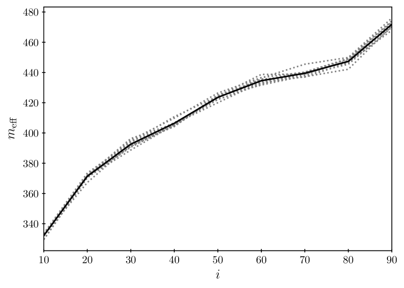
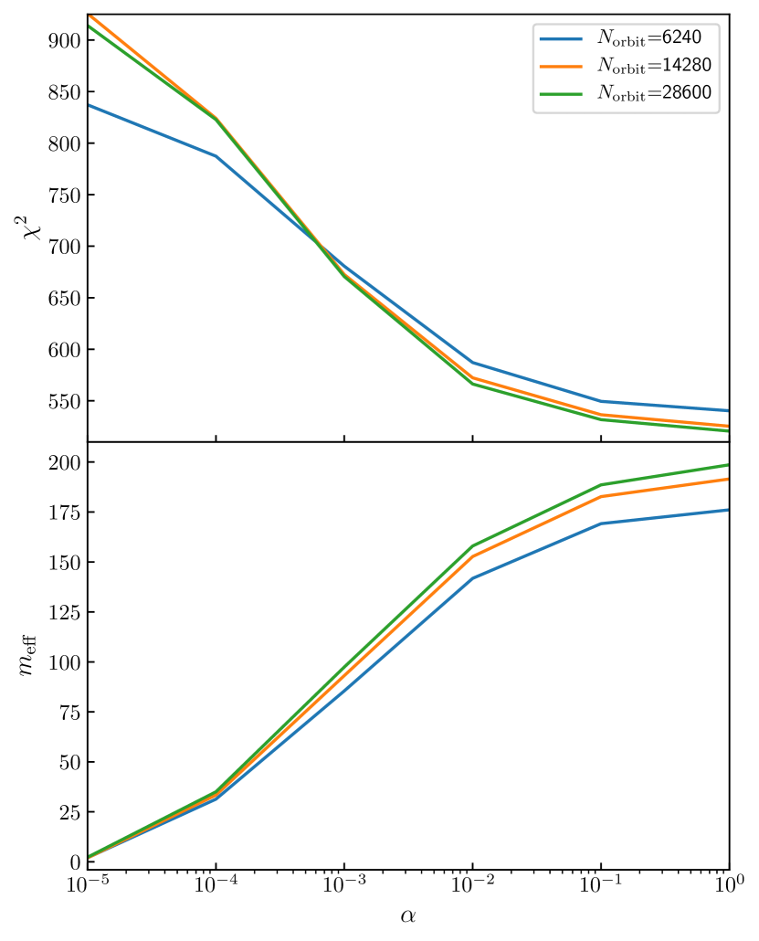
Using the above bootstrap estimation methods we also identified a multitude of other factors influencing the general ability of a Schwarzschild model to fit a given set of data. The most dominant other selection parameter is the regularization value . In Fig. 3 is shown as a function of for three edge-on orbit libraries with different number of orbits . All three libraries are constructed with the correct gravitational potential that was used to create the mock observation they attempt to fit. A decrease in suppresses the freedom of the orbital weights and, thus, restricts the model’s flexibility. In the limit of the model becomes completely rigid resulting in . For very large values of both, and , appear to converge to a constant value. We will come back to the regularization in Sec. 7. An increase in orbits typically leads to a (non-linear) increase in model flexibility, resulting in correspondingly smaller values. However, for very small the orbit library with only 6240 orbits achieves a better even though its intrinsic flexibility is consistently lower than that of the other libraries. This is because all orbit models are very rigid for such small values of and the kinematic data of the toy galaxy shown in Fig. 3 was generated using a maximum entropy Schwarzschild model with exactly . We will describe the construction of such mocks in more detail in Section 5.1.
4 Selection parameter optimisation via model selection
The effective parameters quantify the model flexibility that is synonymous with the size of the parameter subspace accessible to the orbital weights. In principle any selection parameter can influence this freedom, meaning models with different sets of selection parameters should not be be compared without taking into account their actual flexibility. While we showed how we can estimate this flexibility in the last Sec. 3 the question remaining is how we can use this information to choose the model with the best set of selection parameters. Since this means we need to choose the "best" model out of a pool of models with different flexibilities the only option is to work within a model selection framework. We tested three different model selection approaches. The first and what we call intuitive approach is based on the following assumption: if we want to treat all models a priori equivalent then we should demand that the expectation value of our evaluation statistic should be identical for all models. Therefore we should minimize:
| (12) |
because holds for all models that are able to emulate the observed data. The second, information based approach is to maximize the Akaike information criterion (AIC) or equivalently to minimize:
| (13) |
This means that the AIC approach penalizes flexible models more than the intuitive approach in equation 12 does. Since both of the above approaches differ only by the relative importance of the model flexibility , our third, more generalized selection approach is to minimize:
| (14) |
where the factor is a free parameter calibrated using a set of simulations described in the following section 5. Eq. 14 includes the intuitive approach () and the AIC approach () as special cases.
5 Application: Inclination recovery in simulated galaxies
We created a number of toy galaxies with different inclinations to test the model selection framework proposed in the previous section. The goal was to recover their true inclination. Analytical distribution functions for non-spherical models are mostly not very realistic in terms of the orbital anisotropy they imply. Consequently we decided to create the noise-free LOSVDs of our toy galaxies on the basis of Schwarzschild models in realistically flattened 3d mass distributions. This approach is very flexible as modifications to the entropy term can be used to generate almost any desired orbital anisotropy (cf. Neureiter et al. 2021). We cross-checked the validity of this toy model generation on the Hernquist sphere: the modelling results obtained using either LOSVDs from the -body-particle sampled analytic distribution function (Sec. 2.3) or from suitable Schwarzschild models in the Hernquist potential did not show any significant differences. Using this Schwarzschild model construction we simulated the kinematics of both, late-type and early-type galaxies. The former with maximum-entropy models of a realistic mass distribution obtained by deprojecting the surface brigthness profile of a real disk galaxy and the latter with models of a flattened Hernquist distribution. Table 1 is a comprehensive list of all toy galaxies we investigated and their most relevant characteristics. To create realistic mock observations of these toy galaxies the stellar kinematics of the resulting orbit model must be projected to the sky. To this end we projected the kinematics to spatial grids borrowed from real SINFONI and MUSE observations (e.g. Mehrgan et al., 2019) and convolved them with the corresponding seeing. For the early-type galaxies we used a Voronoi grid that covers a large FoV and extends well beyond the toy galaxy’s effective radius. To project the late-type galaxies we used regular grids with a smaller FoV but higher spatial resoultion. The FoV is still large enough to cover the sphere of influence of a hypothetical black hole with a mass typical for the respective galaxy. We simulated 10 independent observations of each toy galaxy by adding random uncorrelated gaussian noise with a standard deviation of two percent of the maximum LOSVD value in the respective spatial bin (cf. Sec. 2.3). Since we generated rotation in some of the toy galaxies (see below) not all of them intrinsically represent a maximum-entropy state.
| Name | Density | Axis ratio q | Angular momentum bias | Inclination | Spatial grid | |
|---|---|---|---|---|---|---|
| Galaxy A | Early-type | 0.6 | 0.0 | 76 | wide field | |
| Galaxy B | Early-type | 0.4 | 0.0 | 76 | wide field | |
| Galaxy C | Early-type | 0.6 | 0.0 | 76 | wide field | |
| Galaxy D | Early-type | 0.6 | 0.5 | 76 | wide field | |
| Galaxy E | Early-type | 0.6 | 1.0 | 76 | wide field | |
| Galaxy F | Early-type | 0.6 | 0.0 | 65 | wide field | |
| Galaxy G | Early-type | 0.6 | 0.0 | 54 | wide field | |
| Galaxy H | Late-type | 0.2 | 1.0 | 30 | intermediate field | |
| Galaxy I | Late-type | 0.2 | 0.0 | 30 | intermediate field | |
| Galaxy J | Late-type | 0.2 | 1.0 | 30 | small field | |
| Galaxy K | Late-type | 0.2 | 0.0 | 30 | small field |
After the addition of noise, all resulting mock observations were modelled with Schwarzschild models using orbits and a regularization parameter of . For our toy galaxies this regularization value was large enough to ensure that has roughly converged to a constant value, in other words the flexibility of the respective models has plateaued and a further increase in does not improve the goodness-of-fit significantly. To recover the mock galaxies’ inclinations, we had to model them under different assumed viewing angles. To do so, we projected the true intrinsic density of each toy galaxy on the sky and deprojected the resulting mock images assuming the various inclinations probed by the dynamical models. For these deprojections we used the Metropolis-Algorithm of Magorrian (1999). It is usually not required to probe every viewing angle as not all inclinations are necessarily compatible with a given photometry. In axisymmetric systems in particular the observed flattening on the sky determines a minimum possible inclination that corresponds to an infinitely thin distribution. But even for triaxial galaxies the range of plausible viewing angles can be narrowed down (cf. de Nicola et al., 2020).
5.1 Simulated galaxies
The early-type toy galaxies have a mass-to-light ratio and are based on the flattened density profile:
| (15) |
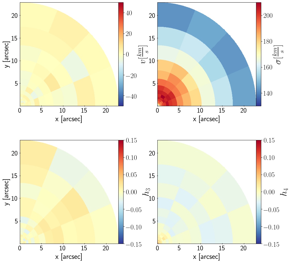
which is similar to the Hernquist sphere (cf. Hernquist, 1990). The variable a parametrizes the spheroidal isodensity surfaces. While not all early-type toy galaxies have the same intrinsic axis ratio q, their total mass , effective radius kpc and distance Mpc are always the same. The density for the late-type toy galaxies was obtained by deprojecting the photometry of a real late-type galaxy (NGC 3489, cf. Nowak et al. 2010). Beyond that we also borrowed the assumed inclination (), distance (Mpc) and seeing from said galaxy for the setup of the late-type galaxies.
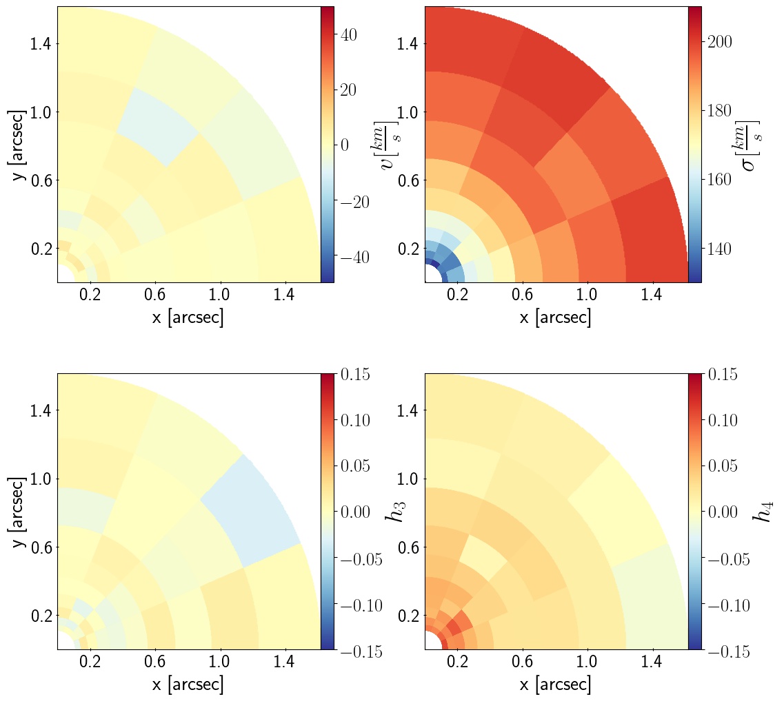
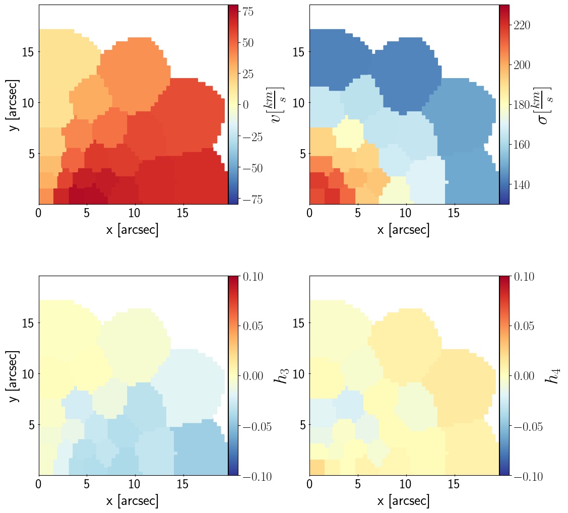
After establishing the density distribution for each galaxy we generated its kinematics by constructing maximum-entropy Schwarzschild models based on this density. The kinematics of the models were then projected onto the sky and convolved with realistic spatial point spread functions (PSF). The (non-parametric) LOSVDs for the early-type galaxies were projected onto a set of 34 Voronoi bins using the method of Cappellari & Copin (2003). To make the mock data as realistic as possible, this observational setup and the respective PSFs were borrowed from real SINFONI and MUSE observations of a massive elliptical galaxy (ESO 325-G004). The mock SINFONI observations cover the inner with high enough spatial resolution to resolve a central supermassive black hole while the corresponding MUSE observations encompass the larger-scale kinematics of the galaxy out to about 2 half-light radii. The typical size of these Voronoi bins varies with radius from about (or ) in the centre to (or ) in the outer bins. An example Gauss-Hermite map for the MUSE grid of one of the resulting mock observations is shown in Fig. 27 in App. B. For the projection of the Schwarzschild kinematics of late-type galaxies we tried two regular grids with differently sized FoVs (cf. Tab. 1) resulting in 30 and 70 spatial bins respectively. For the PSF convolution we borrowed the observed PSFs of the same late-type galaxy NGC 3489 that we used to create the intrinsic density distribution.
All maximum entropy galaxies display characteristic features of non-rotating flattened systems such as smaller observed velocity dispersion and on the minor axis, but overall they behave similar to the spherical toy galaxy of Sec. 2.3 in that their LOSVDs are symmetric and have no net rotation. Since this is not representative of most real galaxies (cf. Emsellem et al., 2011), we also modelled rotating toy galaxies with the goal to investigate how this affects the inclination recovery. We introduced rotation by exploiting the symmetry of our axisymmetric orbit libraries: each orbit of our libraries exists in a prograde and a retrograde version. In a maximum-entropy model, the weights of the two orbits in a prograde-retrograde pair, denoted by and , are identical and consequently the orbits cancel each other’s rotation signal. We can simply manipulate this prograde-retrograde balance to create a toy galaxy with net rotation by reassigning new orbital weights:
| (16) |
Where the free parameter biases the total angular momentum along the library’s symmetry axis. For only prograde orbits contribute to the observed kinematics, resulting in a maximum positive rotation signal, while implies a maximum negative rotation signal as only retrograde orbits are populated. We can also recover our original non-rotating, maximum entropy model by choosing . Using this weight manipulation we created two rotating mock galaxies (see Table 1) with an angular momentum bias of (Galaxy E) and (Galaxy D). In addition to the intrinsic axis ratio q, the inclination i and the angular momentum bias of our toy galaxies we also experimented with a change of the velocity binning by altering the maximum velocity of the LOSVDs while keeping the number of velocity bins constant.
Qualitatively all simulated galaxies showed similar behaviour when modelled under different assumed inclinations. Therefore we first aim to outline this common behaviour using Galaxy D as a generic case. This Galaxy has an axis ratio and was originally projected at an angle , resulting in an apparent axis ratio . In axial symmetry then, inclinations are not compatible with the projected surface brightness and do not have to be considered. When modelling the galaxy, we sampled the inclination parameter linearly in the interval with a step size of .
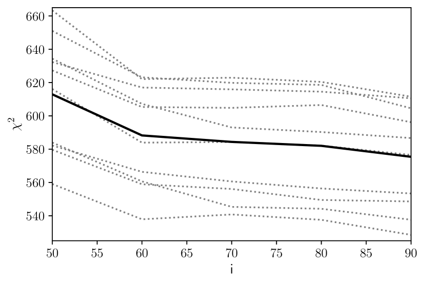
Despite the fact that the galaxy is fairly inclined with a true inclination , the of the Schwarzschild models suggest that the edge-on model is the best fit on average (Fig. 4). This undesired behaviour mirrors the situation in the Hernquist sphere discussed in Sec. 2.3. It is is caused by a drastic change in the model’s flexibility with inclination, as can be seen in Fig 5. The Figure shows that the number of effective parameters increases rapidly as a function of inclination.
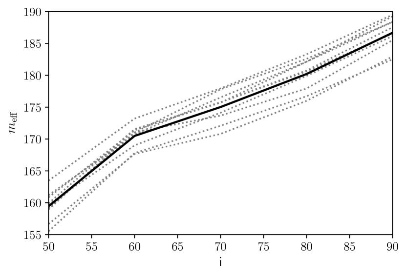
Thus, the lower at higher inclination are not necessarily an indication that the fits to the data are intrinsically better at larger . Rather, the gets lower because the model is more flexible. In other words, the measure for which represents a "good" fit has shifted towards lower values. In fact, if we take the varying model flexibility into account and compare the models within our model selection framework, then the inclination bias disappears (Fig 6). For both, the intuitive and the AIC approach, we can recover the galaxy’s true inclination on average very well. If any, then the fits to the individual mock realisations seem to scatter slightly above the true inclination for the intuitive approach and slightly below the true inclination for the AIC approach, but on average any related bias is very small, . Still, the distribution of the individual fits suggests that even better results might be achieved with some optimized .
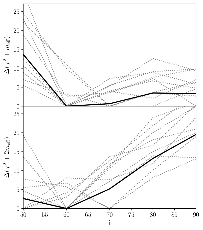
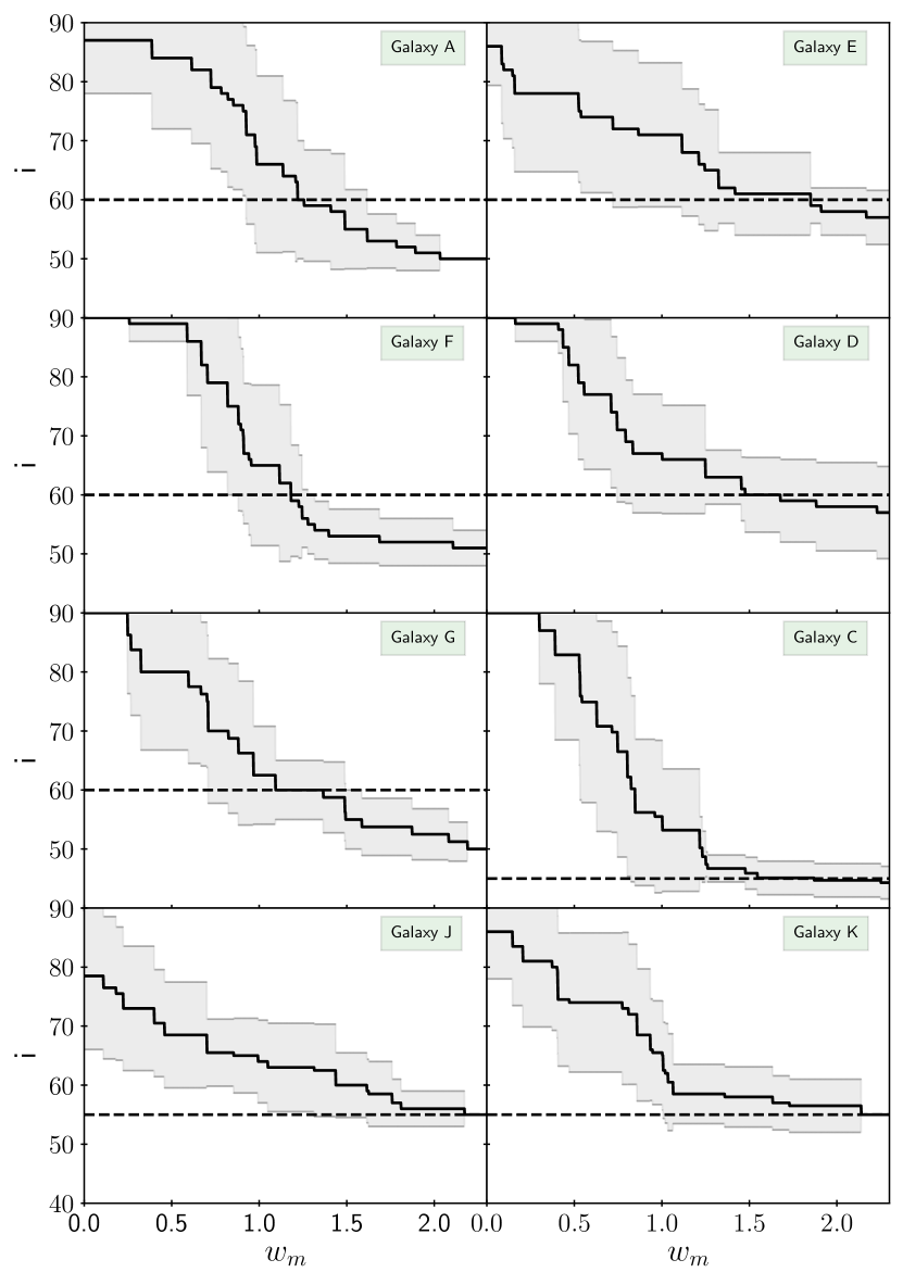
In fact, we repeated this analysis for all toy galaxies of table 1. For a representative subset of these simulated galaxies, Fig. 7 shows the recovered inclination again averaged over fits to ten mock data realisations (solid black lines) as a function of . The Figure shows that the behaviour of the fits to Galaxy D described above is actually generic. For (simple minimization) we find that the "best-fit" inclination is almost always or close to it. With increasing , the influence of the varying model flexibility on the recovered inclination becomes stronger and the "best-fit" inclination moves away from .
For most early-type galaxies, the true inclination is very well recovered with , while larger lead to a slight bias towards too small inclinations. Similarly, the inclination recovery for the late-type galaxies is improved when selecting models with , however, optimum results are achieved in the Akaike regime (). A bias towards too low inclinations is strongly suppressed for the late-type toy galaxies as inclination angles significantly smaller than the true are excluded on the basis of the apparent flattening in the photometric data.
Given the modelling results of all toy galaxies in Table 1 we conclude that a simple minimisation for the selection parameter leads to a very significant bias. This is caused by the fact that edge-on models are much more flexible than models with a lower inclination and, hence, yield much smaller minimum values. However, when taking the differences in model flexibility into account by penalising each model with an additive term proportional to the effective number of free parameters, the inclination recovery actually works very well. With the new model selection framework, we could recover the inclination of all toy galaxies to within on average.
The best results were obtained when weighting the influence of the model flexibility with a proportionality factor of , which is a value right between the "intuitive" approach and the AIC. We will come back to this in Sec. 7 where we also include the regularisation into the analysis.
5.2 Flexibility and underlying galaxy structure
A unique feature of the flexibility of non-linear statistical models is that the number of effective parameters can generally depend on the underlying data generating process (cf. Ye, 1998). In the case of our dynamical models this means that the flexibility is not a universal property of the model alone, i.e. a property of the orbit library, but instead can additionally depend on the underlying galaxy structure.
This dependence becomes especially apparent when comparing the dynamical modelling results of rotating and non-rotating galaxies. We investigated this by fitting mock data sets of a sequence of toy galaxies which were identical except for the angular momentum bias (equation 16). One toy galaxy was generated with and represents a non-rotating maximum-entropy galaxy (Galaxy A in Tab. 1). The two other toy galaxies were constructed to be rotating by setting (Galaxy D) and (Galaxy E). The resulting (noise-free) rotation maps of the latter two toy galaxies are shown in Fig. 8. After having added noise we analysed the three toy galaxies with an identical orbit library and estimated the flexibility of the fits using the bootstrap calculations of section 3.1 above. We repeated this for five different inclinations from to .
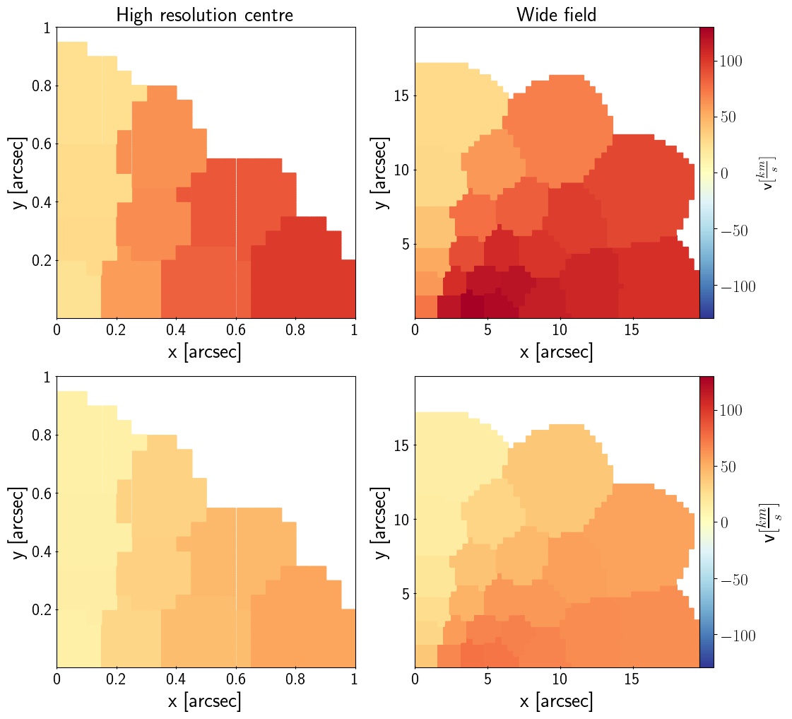
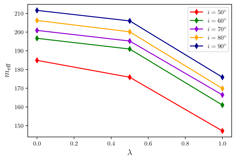
Fig. 9 shows the resulting estimated number of effective parameters. Note that for a given inclination, the mock data of the toy galaxies with different were fitted with exactly the same orbit library. Despite this fact, however, the model’s ability to fit the data changes with . On the one hand, we again see how the overall flexibility of the model increases with . On the other hand, however, we also see that the more net rotation is present in the underlying galaxy, the less flexible the model appears. We argue that the reason for this dependency is the fact, that with increasing rotation the light in the observed LOSVDs is more and more concentrated on either positive or negative velocities. While the amount of light on one side of the LOSVD therefore increases, it decreases on the opposite side and more and more velocity bins in each LOSVD tend to carry only little or even no light when the angular momentum bias is strong. After the addition of Gaussian noise such (nearly) dark velocity bins can formally even carry a negative signal. Since we require the orbital weights to be positive, such formally negative LOSVD values can not be fitted. Thus, because with more rotation more LOSVD bins are prone to carry a negative signal due to noise, the model’s flexibility as estimated by the number of effective parameters will shrink.
This correlation of with the rotation implies that the flexibility of Schwarzschild models depends on the underlying phase-space distribution function of the galaxy under investigation. The same orbit library can be more responsive to one data set than to another. This is in contrast to the flexibility of linear models where the number of free parameters is independent of the underlying data generating process (as long as no constraints on the free parameters are applied). We conclude that the number of effective parameters of a given orbit model should be estimated individually for each new fit. When modelling the kinematics in the different quadrants of the same galaxy separately, for instance, even if one samples the mass parameters from the same parameter grid, the number of effective parameters needs to be estimated separately for each fit in each quadrant.
6 Biases in other selection parameters
The dependence of on the model flexibility is most prominent for differently inclined models, however, in principle any selection parameter can suffer from biases introduced by a variable model flexibility. We investigated this by modelling toy galaxy E with different model inclinations and mass-to-light ratios .
The result is displayed in the top two panels of Fig. 10, which show contours of and as a function of the mass-to-light ratio and the inclination , averaged over 10 mocks. In the direction of the inclination we observe the edge-on bias established in the previous sections. However, the contours reveal an additional bias along the mass-to-light ratio axis. A simple -minimization does not result in a minimum at the true mass-to-light ratio but instead is biased towards slightly larger ratios. The fact that the behaviour is mirrored by the number of effective parameters suggests that this increase in model flexibility causes the bias. While this bias of the mass-to-light ratio is present for all modelled inclinations, it appears to be most significant towards . Thus, a model evaluation based on a simple -analysis would not only overestimate the inclination but would also misjudge the total mass of the system.
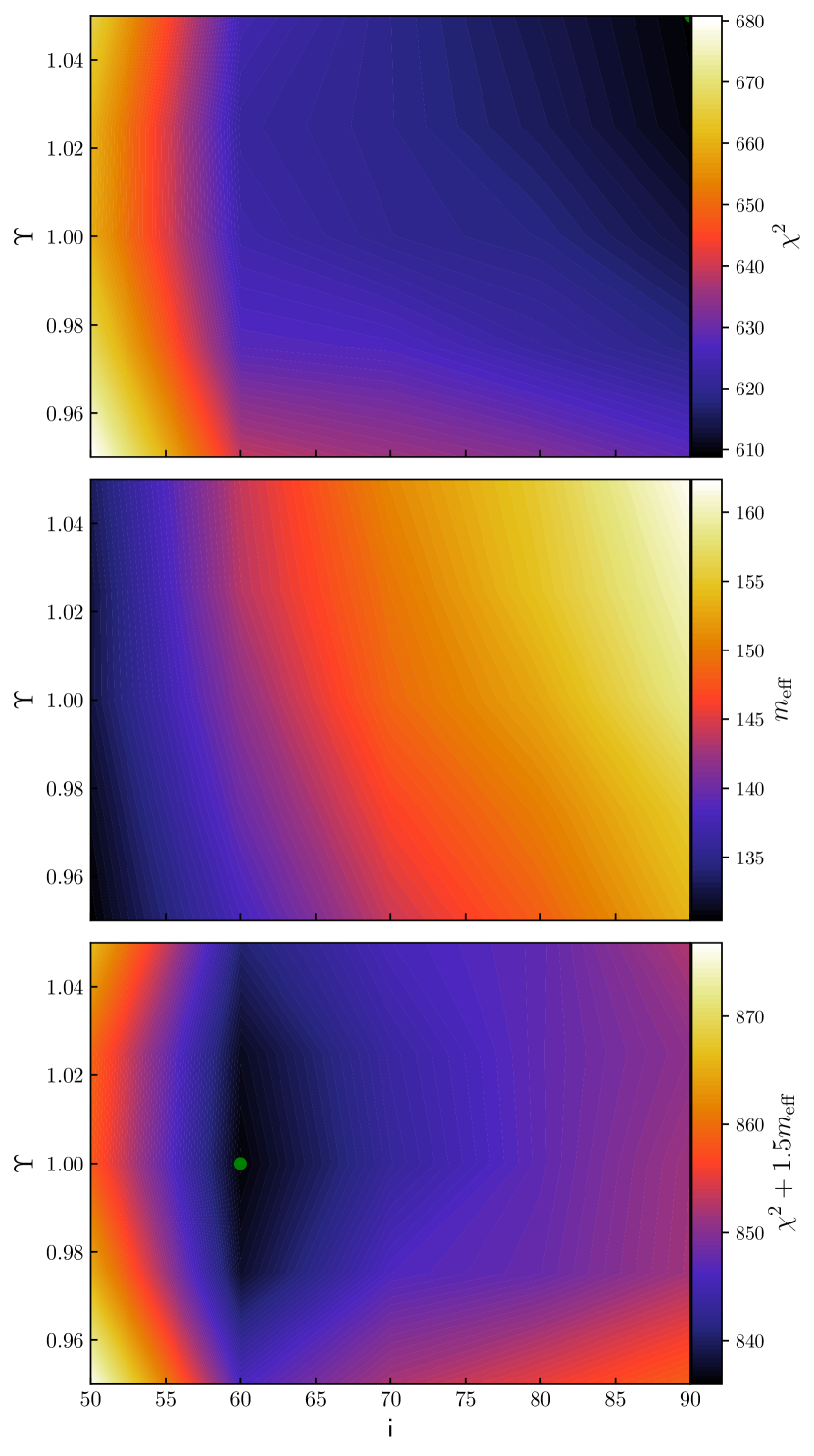
We argue that the reason for this --correlation is due to the higher escape velocity in models with larger total mass. Orbits with a higher escape velocity can potentially occupy velocity bins that are unattainable at lower masses. Models at higher masses will therefore be able to fit more LOSVD bins (if the LOSVDs are sampled out to sufficiently large velocities). This means that they have an increased model flexibility when compared to their lower counterparts.
If we take this effect into account and judge the dynamical models within the model selection framework, then the recovery of the original mass-to-light ratio and inclination becomes highly accurate. This is shown in the bottom panel of Fig. 10 which shows the constraints obtained with the calibrated model selection approach (i.e. Eq. 14). Both inclination and mass-to-light ratio biases have disappeared and the constraints are now tightly centred around the correct model with model and . Similar to the inclination an intermediate calibration weight of proves to be most successful in recovering the correct mass-to-light ratio. The intuitive and the Akaike approach also manage to select the correct model on average, however, their contours are slightly skewed towards larger for and smaller for .
The orbit models shown in this and the previous section 5 were modelled with a fixed regularization . However, the constraining power of the model selection framework for and can be further improved by treating the regularization parameter as an additional selection parameter, as we will demonstrate in section 7.
7 Refinement: The role of the regularization parameter
As mentioned in Sec. 2.2 the regularization parameter is important to control the smoothness of the orbital weights. However, up until now we have simply chosen such that has roughly converged. In the following we will denote such a regularization parameter that was chosen using this convergence criterion as . For the modelling of the toy galaxies in table 1 this happens for , which motivated our somewhat arbitrary choice of . This means we almost only considered the most flexible models as candidate models, since has roughly converged at this regularization value, meaning a further increase in does not significantly reduce further and the corresponding number of effective parameters has plateaued (cf. Fig. 3). While this choice guarantees a good fit to a given kinematic data set, it may not be suitable to restrict our test only to models with such a large as they are prone to overfitting the data. And this, in turn, could potentially weaken the constraints on the selection parameters. Moreover, the optimal weight of the in the model evaluation (cf. eq. 14) could depend on , meaning that a calibration found for one data set of one galaxy may not be applicable to another data set of another galaxy. It is common practice to use Monte Carlo simulations of the galaxy under investigation to determine its optimal smoothing (e.g. Saglia et al., 2000; Cretton & Emsellem, 2004; Thomas et al., 2005; Morganti & Gerhard, 2012; Neureiter et al., 2021). In order to avoid smoothing-induced biases in the models, the mock data should be as realistic as possible and adapted to the particular data set at hand (resolution, signal-to-noise etc.). In addition, since the optimum value of will depend on the underlying galaxy structure such simulations need to be repeated for every galaxy anew. However, a more targeted approach that optimizes directly from the observed data may be advantageous as it would not rely on the choice of mock galaxy that is required for the Monte-Carlo simulations and is supposed to emulate the real galaxy.
For this purpose we again employed the concept of selection parameters. Section 2.1 characterized selection parameters as those that need to be specified to single out an individual model out of the family of models . The respective orbital weights are its free parameters. In general, there may exist many distribution functions (or equivalently vectors w) that satisfy the observational constraints posed by for a given set of selection parameters. The reason is that is not necessarily strictly convex (cf. Neureiter et al., 2021). In practice, this issue is circumvented by adopting a penalized maximum-likelihood estimation by adding a penalty function, such as the entropy term in eq. 5 that makes the solution for the orbital weights unique. However, this means out of all the allowed and statistically viable DFs only a single, privileged DF is identified, a possible issue already pointed out by Magorrian (2006). In the following we will show that our model selection framework facilitates an evaluation of multiple distribution functions compatible with a single set of if we extend the selection parameters to include the regularization parameter .
Which distribution function out of all the compatible DFs (or w) is privileged by a penalized maximum-likelihood approach is determined by the specific value of the weight parameter used for the penalty function (in our case ). In that sense the regularization parameter is a prior that, like the selection parameters, constraints the parameter space available to the orbital weights. Furthermore, like models with different selection parameters, models with different also have varying number of effective parameters. In fact, plays the dominant role in determining the flexibility of a dynamical model, as demonstrated in section 3.1. Consequently, we may attempt to extend the concept of selection parameters to include prior parameters, such as , that push the orbital weights towards certain solutions. The regularization does not necessarily have to be the only such prior parameter that is used to identify a specific DF out all the DFs compatible with a set of selection parameters . For example, it is not necessary to use the phase volumes of the orbits within the entropy-term. Instead one could use a free to bias the solution towards a specific solution (cf. Neureiter et al., 2021). In that case the are simply another set of selection parameters that could potentially be constrained by the establishment of candidate models with different . However, in our case the phase volumes are not themselves independent selection parameters as they are completely determined by the other selection parameters that were used to create an orbit library. Therefore we focus on the regularization parameter that is used to control the smoothness via the entropy term in eq. 5.
If can be thought of as simply another selection parameter, it may be possible to constrain it using the kinematic data by constructing candidate models with various , analogously to any other mass or library parameter. While a recovery using only the kinematic goodness-of-fit is not sensible as it would always favor the maximum models, it may be possible to constrain the regularization by evaluating the models within a model selection framework that takes into account the number of effective parameters. To investigate this possibility we modelled 10 mock data sets of toy galaxy A again, but this time we varied not only the two selection parameters and i, yet also the regularization . Then, as described in Sec. 5, for each model defined by () we estimated and selected the best model via the general model selection approach .
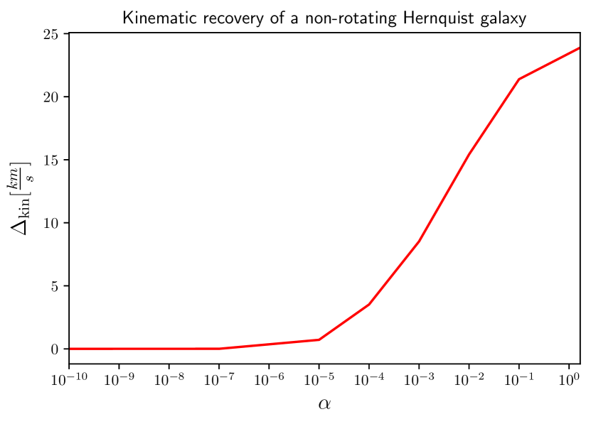
Considering that Galaxy A was created using a maximum-entropy Schwarzschild model with we would expect that an optimal model selection approach should return a model with the same as the best model. The reason is that the orbital weights are uniquely determined if () are given. In general, models obtained with the same and but different will have different orbital weights and so, by construction, should return the weights closest to the input model. The regularization parameter itself is not a physically relevant parameter but simply a choice of prior that restricts the freedom of the orbital weights. However, as a consequence it significantly impacts the form of the resulting distribution function of a dynamical model and its respective kinematic moments. Therefore one should ideally use a regularization parameter that allows the best possible approximation of the true, underlying kinematic structure. To quantify this we characterised the difference between the underlying true orbit model and a fitted model by the average root mean square deviations (RMSD) of the first and second order velocity moments. Apart from the deviations of the individual moments we also define a total kinematic deviation:
| (17) |
Here is the mean stellar rotation velocity of the model around its z-axis, while and are the radial and tangential velocity dispersions.
Fig. 11 shows versus when the inclination and mass-to-light ratio are fixed at the correct values. Obviously, the input model is exactly recovered for the lowest . Larger values lead to a larger discrepancy between the fitted velocity moments and the ones in the input model. The reason is that with increasing the model starts to overfit the noise incorporated in the mock data.
In analogy to Sec. 5, where we used the accuracy of the inclination recovery as criterion to decide upon the optimal weight factor in we can now also include in the optimisation of . Fig. 12 shows the median and mean values of the selected models for each mock of Galaxy A as function of the calibration weight .
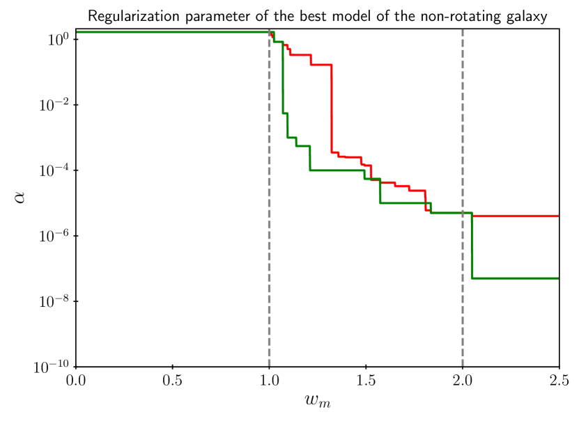
Unsurprisingly the simple minimization selects the model with largest sampled , in this case 1.67, meaning the best models overfit the noise and the recovered distribution function has a higher degree of irregularity than the smooth input model. For larger we approximate the input model better as the median shifts from to for . In the regime of the Akaike approach, the selection framework yields . In terms of the quality of the reconstruction of the internal velocity moments, any in this regime leads to an almost perfect recovery of the input model (Fig. 11).
While the model selection framework with a variable seems to work very well for the mocks of Galaxy A, in particular the Akaike approach, it may not be the most realistic setup. For one because the generating model for Galaxy A is a maximum entropy model without any rotation, but mainly because one can generally not expect to have the "true" generating model among the tested models, which in the case of Galaxy A is the model with selection parameters , , . Furthermore the generating model of Galaxy A is also the model with the smallest number of effective parameters and consequently the selected model is always the generating model one as long is chosen big enough, meaning that we only establish a lower boundary for the calibration weight .
For these reasons we additionally tested the approach with a variable regularization on the mocks of Galaxy D, which is a rotating toy galaxy with an angular momentum bias of . In this case the best regularization parameter is not known in advance and the generating model is not necessarily among the tested models.
Fig. 13 shows the median and mean regularization parameter of the best model of Galaxy D as a function of the calibration weight . We find large for followed by a steep falloff that turns into a stable plateau for , similar to Galaxy A. However, the optimal for the Akaike approach is now at an intermediate and not where the models have the smallest number of effective parameters. (Only for the approach tends towards models that simply have the smallest number of effective parameters. However, such large can easily be discarded because they lead to unreasonably large , i.e. they are unable to fit the mock observations of Galaxy D).
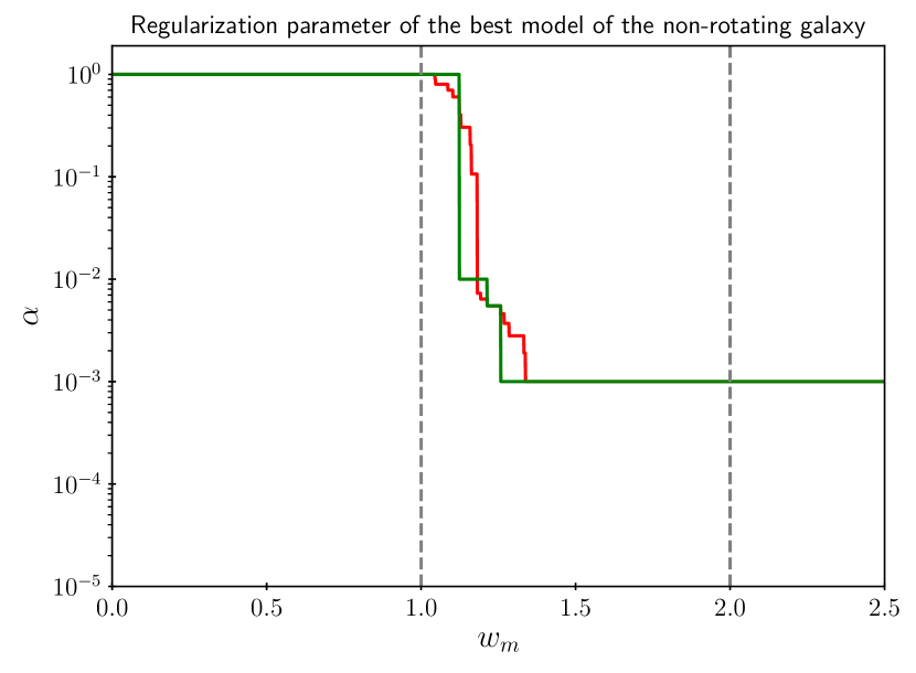
The model selection framework with suggests that the optimal amount of regularization for Galaxy D is achieved with . It becomes evident from Fig. 14 that models with this regularization of are indeed the models that reproduce the intrinsic velocity structure of Galaxy D best.
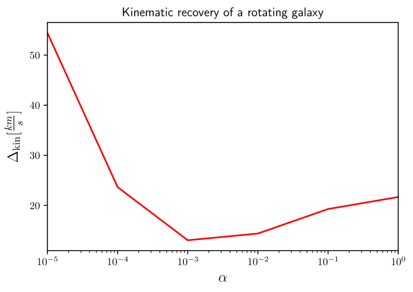
This demonstrates that the model selection framework with leads to an optimal recovery of the velocity structure of Galaxy D. Less regularized models, while nominally achieving a better , overfit the LOSVDs and do not improve the recovered velocity moments. On the other hand more regularized models with are not sufficiently flexible to be able to describe the underlying non-maximum entropy distribution function.
Treating the regularization as an additional variable selection parameter within our model selection framework, instead of arbitrarily fixing it to some value, does not merely affect the recovery of the intrinsic kinematics but also improves the constraining power of the other involved selection parameters. This is illustrated in Fig. 15 and Fig. 16, which show the average, recovered mass-to-light ratio and inclination of Galaxy D for different model selection frameworks for two cases: (i) the often adopted approach where the smoothing parameter is fixed to some value (Fig. 15, where is fixed to 1) and (ii) the more general case where is a variable model parameter (Fig. 16).
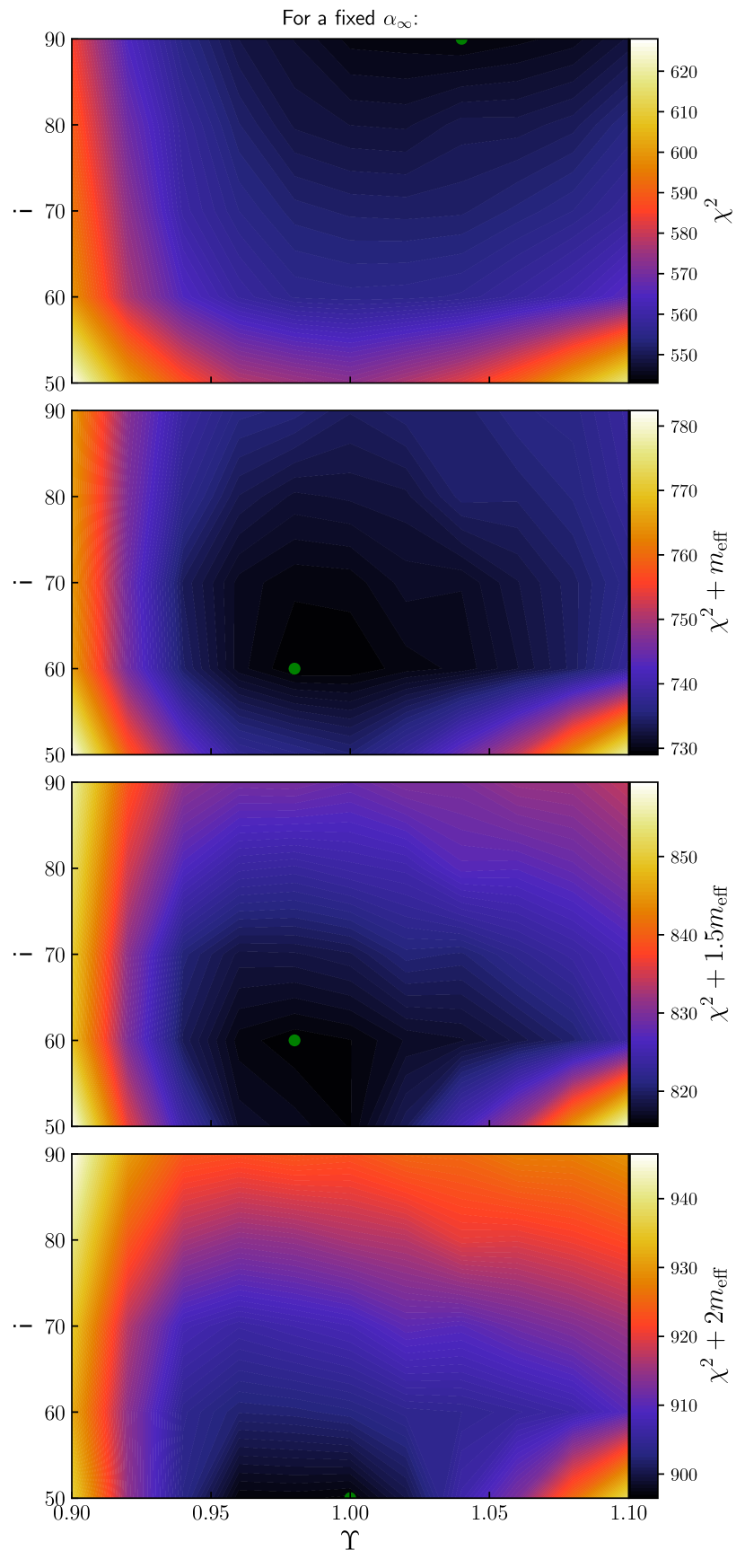
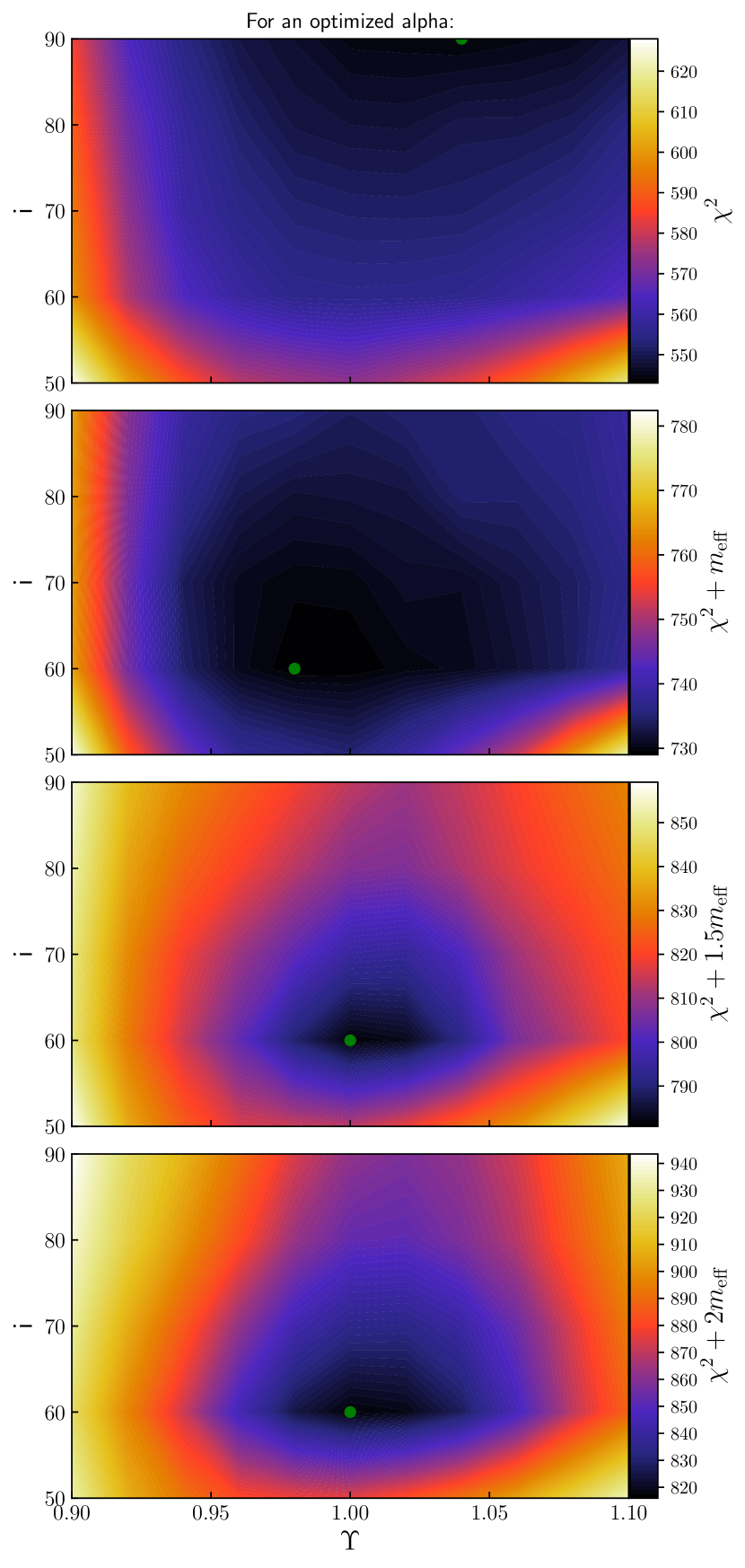
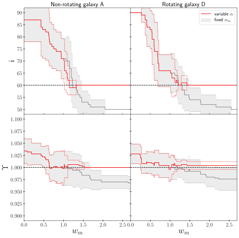
As established in section 6, a simple minimization results in an overestimation of the mass-to-light ratio of about - and an edge-on viewing angle for both, the modelling with fixed and the one with variable . Only when the varying number of effective parameters of candidate models are accounted for with the model selection framework , one can find the correct selection parameters and . The constraining power of the model selection framework significantly improves if the regularization is treated as a selection parameter. In addition, the results are more stable with respect to the calibration weight . In fact, compared to the case with fixed regularisation, the Akaike approach yields unbiased results when the amount of regularisation is optimized during the fit. This is further illustrated in the top panels of Fig .17, where we show the average recovered selection parameters and against the calibration weight for Galaxy A (left) and Galaxy D (right). With optimized regularisation, the model selection results are stable beyond , while modelling runs where we kept the regularisation to a fixed value developed a bias to less flexible models beyond . For the modelling with variable in the Akaike regime we further note a significantly reduced scatter of both and that appears to become smaller than our sampling steps.
Given the strong improvements on the constraints for the global selection parameters, we now investigate the intrinsic velocity distributions (the orbital anisotropy) under optimized regularisation. In Fig. 18 we show the total kinematic RMS deviations of the best models to Galaxy A and D with respect to the kinematics of the generating model. The Figure also includes the RMSDs of the net velocity and the anisotropy parameter .
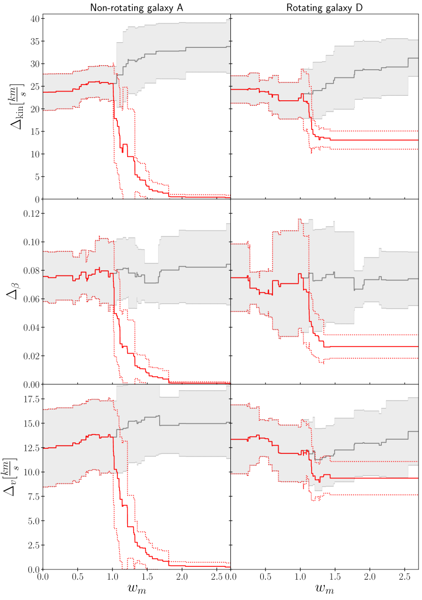
For both galaxies the approach with fixed and variable regularization are initially congruent for small as the model selection is dominated by and consequently, even in the case of variable regularisation, models with values as large as the one that we assumed for the fixed regularisation case are favoured. When is fixed, an increase of beyond counteracts the inclination and mass-to-light ratio biases, while the recovery of the intrinsic kinematics does not improve. For a "sweet-spot" appears, where the correct inclination and mass-to-light ratio are obtained on average. This is in line with our calibration of the optimal in for described in Sec. 5. A further increase of overcompensates the mass-to-light ratio and inclination biases, suggesting that the choice of the specific model selection framework would be crucial when modelling real galaxies.
Remarkably, the choice of the calibration weight is simplified when the candidate models are optimized with respect to the degree of regularization: the correct selection parameters are recovered for a wide range of , including the Akaike . Moreover, the recovery of the intrinsic kinematics, i.e. the rotation and the anisotropy in the second order velocity moments, of both toy galaxies have significantly improved by treating the regularization as an additional selection parameter in the construction of the candidate models. With the right model selection, the intrinsic anisotropy can be recovered more accurately with uncertainties no larger than in the mean.
Simply fixing the regularization complicates rather than simplifies the selection of the best candidate model and in the worst case may even skew the results for other selection selection parameters. Therefore dynamical modelling of galaxies with an a priori fixed amount of regularization should be avoided if possible. For example, Thomas et al. (2007b) show for their sample of Coma galaxies that whether a galaxy is radially anisotropic or tangentially anisotropic is rather independent of the assumed regularisation. However, the strength of the actual anisotropy, i.e. how much radial or how much tangential the orbit distribution is, does indeed depend on the amount of regularisation applied in the models.
8 A real Galaxy: Dynamical Modelling of NGC 3368
We now turn to the application of our model selection approach to the real galaxy NGC 3368. This galaxy is part of the SINFONI black hole survey (cf. Saglia et al., 2016) and was chosen by us as follow-up of a previous analysis by Nowak et al. (2010).
Due to the fact that NGC 3368 is a disk galaxy, its inclination can be estimated independently of the dynamical modelling. It is therefore a useful testbed for the inclination recovery. The observed ellipticity of the outer disk implies a minimum inclination of for an axisymmetric razor-thin disk. Assuming a typical (intrinsic) disk axis ratio of , NGC3368 is expected to be inclined at a slightly larger angle of to project to the observed ellipticity. Nowak et al. (2010) also estimated the inclination of NGC3368 via the Tully-Fisher relation, which yields .
In section 8.1 we will provide a short overview of the imaging and spectroscopy data. More details can be found in Nowak et al. (2010). Section 8.2 reviews the modelling results obtained from a traditional minimisation at fixed regularization. Model selection results with optimized regularisation follow in Sec. 8.3.
8.1 Overview - Photometric and kinematic data for NGC 3368
NGC 3368 is a double-barred spiral galaxy with a composite bulge consisting of a larger pseudobulge and a smaller classical bulge (cf. Erwin, 2004). The galaxy is classified as a LINER2 (Ho et al., 1997). The activity is so weak that we do not expect it to influence the dynamical modelling results. We assume that NGC 3368 lies at a distance of (Tonry et al., 2001) where 1 corresponds to .
The SINFONI kinematics of NGC 3368 were obtained with the K-band grating in the resolution mode. The average adaptive-optics corrected PSF had a FWHM of . Non-parametric LOSVDs were obtained from the CO bandheads adopting the approach of Gebhardt et al. (2000). More details on the data reduction process, AO correction, selection of template stars, and the resulting kinematic maps of the galaxies can be found in Nowak et al. (2010).
The photometry acquired for NGC 3368 is a combination of different data sets: Sloan Digital Sky Survey observations (York et al., 2000) in the r-band were used to find the ellipticities of the outermost parts of the galaxy’s disk. Intermediate radii of NGC 3368 are mostly covered by a dust-corrected HST NICMOS2 F160W image and a K-band (2.2) image of Knapen et al. (2003) observed with the Isaac Newton Group Red Imaging Device (INGRID). The photometry is completed by the collapsed K-band data cube images taken with the integral field spectrograph SINFONI at the Very Large Telescope (VLT). For more detailed information on the image matching, seeing, dust-correction and an isophote analysis see Nowak et al. (2010).
As noted before, the photometric bulge of NGC 3368 has a composite structure. The central 2 are dominated by an almost round and kinematically hot "classical" bulge. Outside this region a more flattened and kinematically cooler structure emerges: the disky pseudobulge. Since the SINFONI FoV has a size of , both components are relevant for the modelling. To account for potentially different mass-to-light ratios in the respective stellar populations, we deproject the classical bulge separately from the pseudobulge and assign each deprojection its own mass-to-light ratio . To this end, we adopt the photometric bulge-disk decomposition of Nowak et al. (2010). It assumes that the disky pseudobulge is the inner extension of the galaxy’s large scale disk and both are combined into the photometric disk component. The other photometric component, respectively, consists only of the "classical" bulge. In practice, the deprojections were again obtained using the Metropolis-Algorithm of Magorrian (1999) without any shape prior. Non-axisymmetric features in the photometric data, like bars and spiral arms, are averaged over as described in Nowak et al. (2010). We tested a grid of assumed inclinations ranging from to . In the following we simply refer to the classical bulge component as the bulge, and the pseudobulge+disk as the disk component.
8.2 -modelling of NGC 3368
This section illustrates the results of the "traditional" dynamical modelling approach for NGC 3368, which is based (i) on evaluating different mass models based on a pure -analysis (i.e. assuming ) and (ii) on a fixed strength of the regularisation. These results are later contrasted to the model selection framework with optimized regularisation (Sec. 8.3).
For our final mass model we add a central SMBH to the two stellar mass components:
| (18) |
where and are the luminosity densities at assumed inclination . For the analysis of this Section we considered only two inclinations: and . A denser inclination grid is used for the model selection approach (Sec. 8.3). Even though it seems likely that a considerable amount of the total galaxy mass is contributed by a dark matter (DM) halo, the addition of a DM component to this model of the galaxy center is not required. Erwin et al. (2018) demonstrated that the addition of a DM halo to a two-component stellar model of (the inner parts of) a disk galaxy neither improves the fit significantly, nor does it change the black hole mass or bulge mass-to-light ratio drastically. It’s only that the disk mass-to-light ratio of such a two-component model without DM is larger than the of a mass model that does include DM (and probably larger than the actual of the stars in the disk). This is because the disk "absorbs" the dynamical role of the ignored dark mass, which leads to a that is biased high.
With the above mass model we constructed trial models by varying the three traditionally relevant selection parameters that determine the orbit library: the mass-to-light ratios of bulge and disk, the black hole mass. With the goal to achieve an efficient, yet nonetheless sufficiently dense sampling of these parameters we narrowed down the approximate location of the minimum with an initial round of trial models that sparsely sampled a wide range of mass parameters. Using the information gained from this initial minimization we decided for the following final sampling grid: The black hole mass is sampled linearly in the interval [, ] with a stepsize of and the bulge mass-to-light ratio is linearly sampled 15 times in the interval [, ]. It turned out that the SINFONI FoV is too small (inner of the galaxy) to constrain . Therefore we decided to sample only to save computation time. This indeterminacy of was already noted in Nowak et al. (2010). For the smoothing we applied the old approach to set guaranteeing that has converged.
Estimating the statistical errors of the dynamical models is non-trivial, mostly because unlike in our toy galaxies, the measurement errors of real LOSVDs are strongly correlated (e.g. Houghton et al., 2006). If these correlations are unknown or neglected then the calculated is systematically smaller than (cf. Tabs. 2 and 3). The absolute values and, consequently, also the significance intervals become inaccurate then. Ideally this issue could be solved by taking the full covariance matrix of the observations into account in the modelling, we plan to investigate this in the future. Another way to circumvent the issue would be the modelling of multiple observations of the same galaxy. Then one could calculate the RMS of the recovered selection parameters, analogously to the modelling of 10 different mocks of our toy galaxies (e.g. Sec. 5). In practice, this is unfeasible. However, if the investigated galaxy is perfectly axisymmetric then each quadrant provides essentially an independent observation of the same underlying galaxy structure. This simple approach of error estimation can also be adopted for galaxies that deviate from axisymmetry, in which case the resulting RMS will be increased by the systematic structural differences between the quadrants (cf. Nowak et al., 2010; Rusli et al., 2013).
Fig. 19 illustrates the resulting constraints for the mass-to-light ratios and black holes mass for both, the models and the models in the four galaxy quadrants.
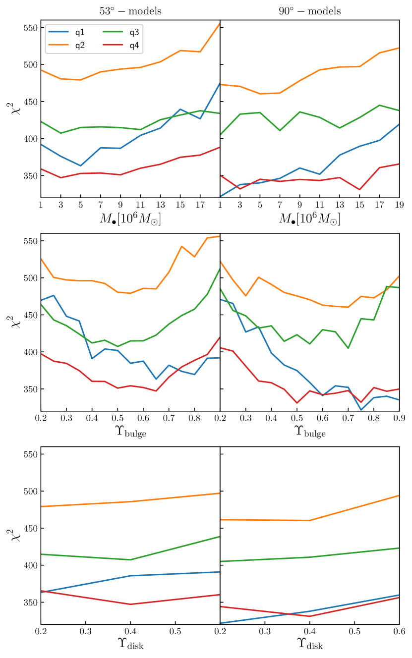
The models obtained under an assumed inclination of (motivated by the disk flattening as described above) yield black hole masses . The formal average over the four quadrants is . However, in some quadrants black hole masses of up to are hardly ruled out when looking at the detailed curves. The mass-to-light ratio of the bulge is well constrained with an average value of . As already mentioned, the disk mass-to-light ratio is essentially unconstrained by the SINFONI kinematics. The constraints for the black hole mass at are much noisier than at . Averaged over the four quadrants, we find (with a more than five times larger scatter than in the case). In fact, neither very small black black hole masses nor very large ones can be ruled out at a significant confidence level. While we do not observe such a strongly increased scatter in we do see evidence for a slight shift towards larger mass-to-light ratios when modelling the galaxy edge-on: .
In the case of NGC 3368 the observed disk ellipticity strongly suggests that the models at are more realistic than the ones at , but we do not have such prior information about a galaxy’s inclination in every case, in particular not if it is a generic early-type galaxy. In that case one would be reliant on the values of the differently inclined models. Table 2 shows the selection parameters and corresponding minimum values of the best fitting model for each quadrant and inclination. In all quadrants, the edge-on models have a lower value than the models at . In other words, if NGC 3368 would be modelled without external knowledge about its inclination a pure analysis would erroneously conclude that the galaxy is seen edge-on, when, in fact, an independent inclination measurement would indicate .
| Quadrant | i | |||||
|---|---|---|---|---|---|---|
| 1 | 0.65 | 0.20 | 5.0 | 363.230 | 0.3844 | |
| 2 | 0.55 | 0.20 | 5.0 | 479.117 | 0.5070 | |
| 3 | 0.50 | 0.40 | 3.0 | 407.302 | 0.4310 | |
| 4 | 0.65 | 0.40 | 3.0 | 347.183 | 0.3674 | |
| 1 | 0.75 | 0.20 | 1.0 | 321.628 | 0.3403 | |
| 2 | 0.70 | 0.40 | 5.0 | 460.396 | 0.4872 | |
| 3 | 0.70 | 0.20 | 1.0 | 405.026 | 0.4286 | |
| 4 | 0.50 | 0.40 | 15.0 | 331.003 | 0.3503 |
These results are not surprising. In Sec. 5 we have seen that a simple minimisation tends to yield results that are biased towards . Moreover, in Sec. 6 we have seen that this inclination bias comes along with a noticeable mass bias (of the order of 10 per cent). Assuming that NGC3368 is seen under an inclination angle close to the expected , than our analysis of NGC3368 is fully consistent with our expectations based on the simulated toy galaxies discussed in the previous Sections.
8.3 Model selection of NGC 3368
In Sec. 7 above, we have demonstrated that the most accurate reconstruction of a galaxy’s mass distribution and internal structure is achieved when using a model selection approach rather than a simple minimisation. Moreover, treating the regularisation strength in a similar way as other selection parameters turned out (i) to improve the accuracy of the galaxy reconstruction and (ii) to reduce the sensitivity of the results on the weight for the effective parameters . Here, we transfer this approach to NGC3368 and minimise . The choice for the Akaike weight directly follows from the results of Sec. 7. We adopt the same mass model (Eq. 18) as for the analysis in the previous Sec. 8.2, consisting of a central black hole, a disk and a bulge. Neglecting potential effects of the deprojection degeneracy this implies that the orbit models are completely determined by the 5 selection parameters , , , , . However, in order to reduce the computation time we restricted ourselves to models with a fixed , since is almost unconstrained over the SINFONI FoV (Fig. 19).
Fig. 20 shows that the optimal amount of regularisation is well constrained by the data: within the Akaike model selection framework all four quadrants of NGC 3368 are best modelled with an intermediate regularization of . Fig. 21 shows the corresponding constraints for , and (all results are listed in Tab. 3).
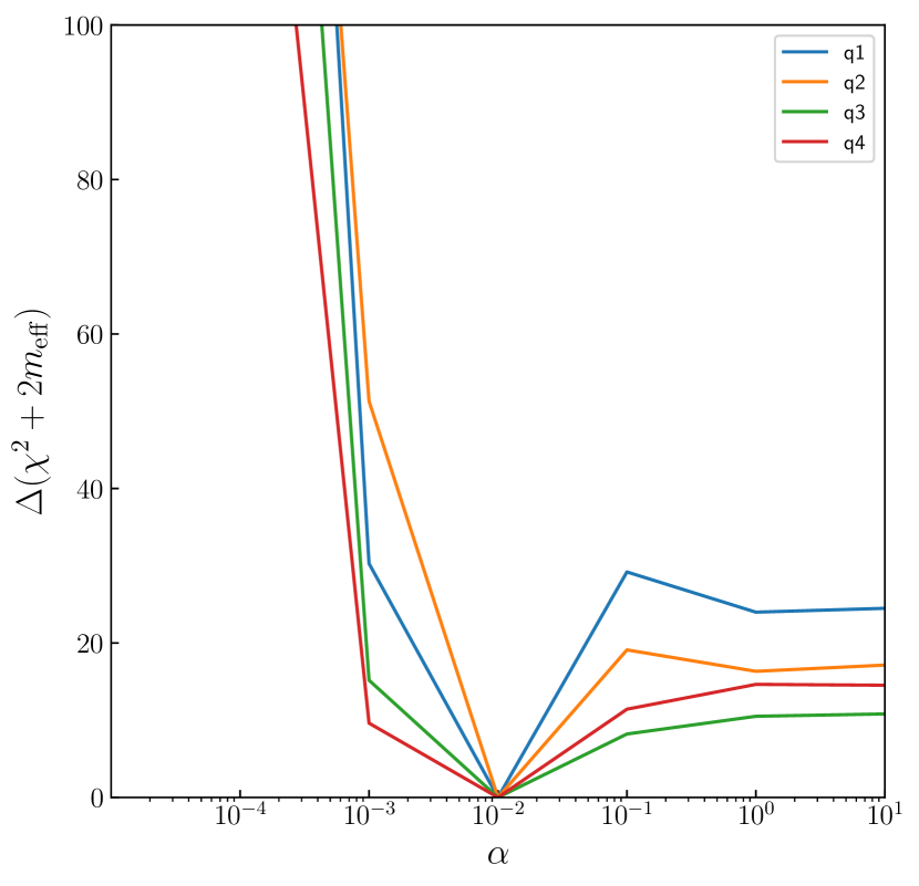
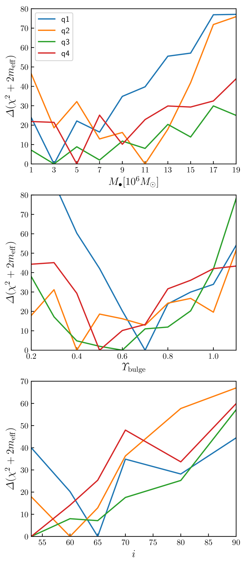
| Quadrant | i | ||||
|---|---|---|---|---|---|
| 1 | 65° | 0.7 | 3.0 | 861.02744 | |
| 2 | 60° | 0.4 | 11.0 | 934.158201 | |
| 3 | 53° | 0.6 | 3.0 | 882.207510 | |
| 4 | 53° | 0.5 | 5.0 | 812.338033 |
Averaging the modelling results of the four quadrants we find that the AIC estimation yields a black hole mass of , a mass-to-light ratio , and an inclination angle . Compared to the results of the simple -minimisation in Sec. 8.2 we immediately see that the inclination bias has disappeared. The model selection approach with optimized regularisation yields an inclination that is consistent with the inclination angle derived independently from the disk flattening. This result was expected after the analysis of the toy galaxies above. Still, it is somewhat astonishing given how small the FoV of the SINFONI kinematic data actually is. However, this underlines the power of the model selection approach to extract all the information contained in the 945 measured LOSVD data points in each quadrant. Another difference to the simple minimisation is the fact that the model selection approach yields a 10-15 percent smaller . Again, this is fully consistent with the toy galaxy results, where the recovered masses were biased high by up to percent when a simple minimisation was performed, while there was no mass bias in the model selection framework. The only significant difference to the simulation results is that the scatter in of NGC3368 is not reduced in the model selection framework compared to the minimisation. This could be caused by a multitude of issues:
-
1.
Systematic differences between the quadrants of NGC 3368 reflecting the galaxy’s intrinsic non-axisymmetry.
-
2.
Inaccurate errors of the observed LOSVDs.
-
3.
Negligence of the correlations between the measurements of the same LOSVD at different line-of-sight velocities in the modelling and bootstrap iterations.
-
4.
A potential non-alignment of disk and bulge.
We used an updated version of our axisymmetric Schwarzschild code for this analysis, compared to Nowak et al. (2010). Therefore, the results of the pure analysis can not be compared easily. However, we note our black hole mass is slightly smaller than the quoted in that paper while our is about 25 per cent larger. These small discrepancies could also partly be caused by the different choice of mass parameter sampling and regularization.
After selecting a dynamical model with AIC one should always confirm that the selected model can in fact reproduce the observed data well as AIC only compares the models relative to another but makes no statement about their absolute quality. Fig. 22 demonstrates this for the models of NGC 3368 by showing the major-axis kinematics of the best AIC and models in relation to the observed SINFONI data. The errorbars for the SINFONI data are the errors estimated from uncorrelated Monte-Carlo realisations of the non-parametric LOSVD data, thus, they are slightly underestimated. Both, AIC and models, fit the data well. However, as one would expect, the AIC model appears to be slightly smoother. It does not react to outliers as much as the models do. Instead of a validation by eye as done here for the major axis of NGC 3368, it may be advantageous to cross-check the goodness-of-fit of AIC models more systematically by confirming whether holds for the selected models (cf. the discussion in the next Sec. 9). However, this is not a viable option as long as the correlations in the real LOSVDs are not implemented in the calculation of and as this causes both values to be underestimated.
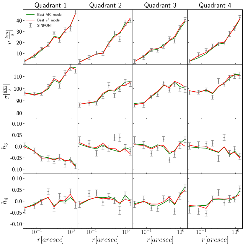
9 Discussion
In the following we examine the statistical objective of AIC model selection in the context of dynamical modelling and address potential problems that may arise when estimating intrinsically degenerate properties with AIC (Sec. 9.1). Subsequently we review earlier studies attempting an inclination recovery using axisymmetric models (Sec. 9.2) and discuss the implications for the mass reconstruction when selecting models based on their alone (Sec. 9.3).
9.1 Model selection and intrinsic degeneracies
The toy galaxy recoveries discussed in Secs. 5 and 7 had in common that the selection parameters under investigation had a unique "true" value. In the model selection setup, this true value could be recovered in an unbiased way with high precision. In order to assess how the model selection framework operates in a degenerate case where such a true value does not exist, or where the data is insufficient to constrain a selection parameter, it is useful to get back to the example of the inclination recovery in a sphere (cf. Sec. 2.3): in a kinematically isotropic sphere all viewing angles should be equivalent. Fig. 23 shows and versus the inclination for the same N-body models as in Fig. 1 (cf. Sec. 2.3). At each tested inclination we optimized the regularization strength as in Sec. 7. Apart from the regularization we only varied the inclination, meaning that the orbit libraries are the exact same for all models. In contrast to the non-spherical toy galaxies that we tested in the previous sections, the AIC approach now appears to be biased, in the sense that it prefers low inclinations although all viewing angles should be equivalent (lower panel of Fig. 23). The "intuitive" model selection framework displays the degeneracy one would generally expect for a spherical model: no inclination is preferred over the other (upper panel of Fig. 23). We will come back to this below.
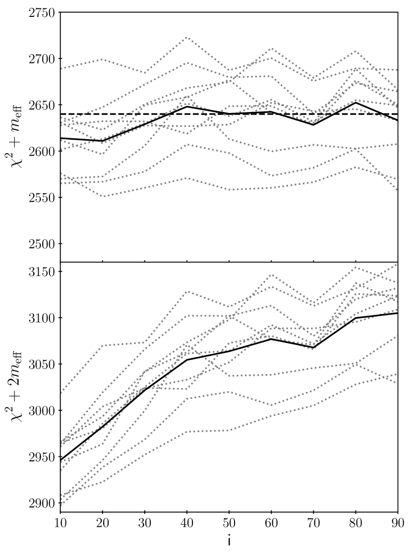
The reason why AIC assesses models of a spherical galaxy differently depending on the inclination can be understood by elaborating what the Akaike criterion is designed to achieve in a more general, statistical sense. Coming from information theory AIC estimates the information loss when modelling an underlying structure/process with a statistical model and selects the model that has the least information loss. The information loss of a statistical model is generally quantified by the Kullback–Leibler divergence (KLD) between the fitted model and the underlying (noise-free) structure it is supposed to represent. Naturally, since the latter is usually unknown, AIC is merely an estimate of the actual information loss.
When transferring these considerations to the context of dynamical models it is crucial to clarify what the statistical model and the underlying structure actually are in this case. The data being fitted by dynamical models are the observed kinematic data, implying that statistically speaking the underlying structure are the noise-free LOSVDs and not the galaxy’s distribution function or mass structure. Analogously, the statistical model is not the orbit model itself but is given by the LOSVDs it produces (cf. Sec. 2). The internal structure of the model, i.e. how one arrives at , is only of secondary concern when evaluating the models.
What this means for the modelling of the isotropic N-body sphere is that the AIC is supposed to minimize the differences between the model LOSVDs and the true LOSVDs. As mentioned above, this difference is quantified by the KLD from to but can also be illustrated more heuristically by the RMSD of the LOSVDs.
As shown in the top panel of Fig. 24, behaves indeed very similar to (cf. Fig 23): both have their minimum where the orbit library is viewed close to face-on.
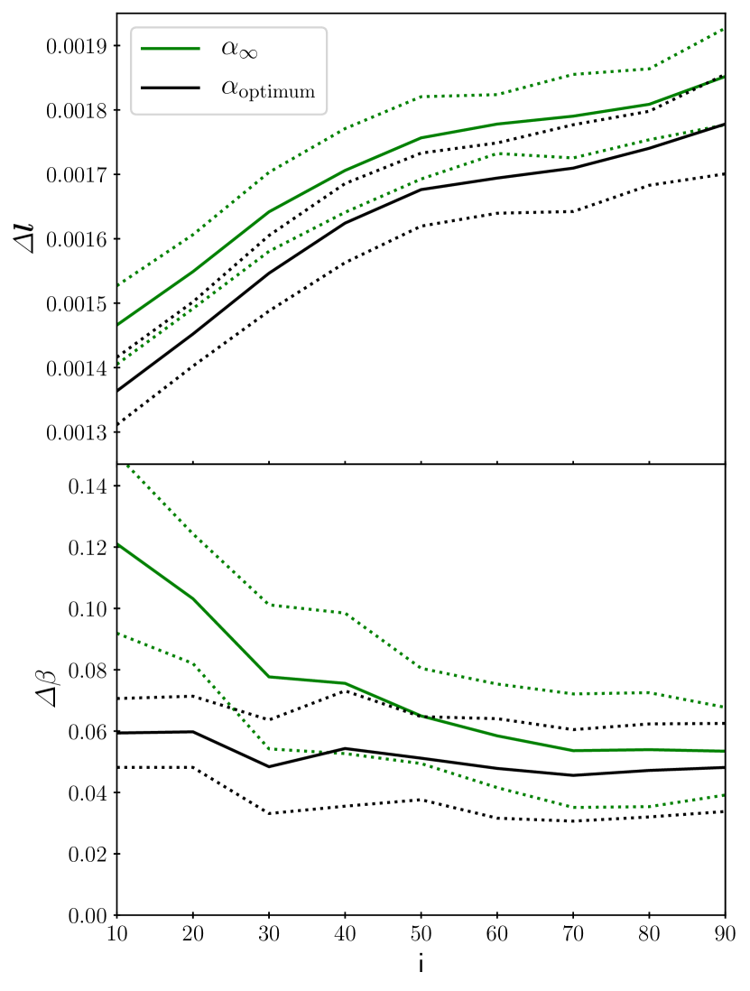
In that sense the AIC selection achieves exactly what it is intended to do, namely to select the model that emulates the underlying LOSVDs best. That the true LOSVDs happen to be represented slightly better at one inclination than another is related to the design of our model. While the sphere itself has no preferred viewing angles, our axisymmetric model does have such a preferred axis. E.g., while we have pairs of orbits that only differ in the sign of we do not have the equivalent pairs of orbits that only differ in the sign of other angular-momentum components. We expect that an orbit sampling using a 5d starting space (Neureiter et al., 2021) will lead to a different behaviour with respect to the assumed viewing angles in a sphere.
Irrespective of the question which particular inclination happens to yield the best LOSVDs we can ask whether a selection parameter (here: the inclination) is constrained by the data or not. As already mentioned above, the top panel of Fig. 23 shows that at all inclinations. This is exactly the expected behaviour when the data does not constrain the exact value of : For a viable statistical model we expect (Sec. 3) and if this can be achieved for all , then the data does not constrain the inclination. Among all these viable models the model selection picks up the one with the smallest . This is a generic result, because when , then
| (19) |
In other words, when a selection parameter is not constrained by the data and over some extended interval, then the model selection may be biased in the sense that it will pick up that particular model inside the interval which has the lowest .
In terms of the selection parameter recovery such a bias is undesirable. However, as we have seen above, it still comes along with a reduction of the information loss in the statistical model. One can therefore also ask how it affects other intrinsic properties of the orbit model. Unsurprisingly, it does not necessarily entail an improvement in these intrinsic properties either as they are also not subject to the AIC optimization. However, in practice, it often does improve the situation. It should be noted that in general, a model’s intrinsic properties (like the orbital anisotropy) are only meaningful when a priori knowledge about a galaxy’s typical structure is added. In principle, any could be a good statistical model without the need of secondary properties such as inclination, orbital weights etc. (cf. Sec. 2). An improvement in such secondary properties can only be achieved if a property correlates with an improvement of the model LOSVDs, or in other words: if the property can be constrained by ideal (noise-free) data. As an example, the bottom panel of Fig. 24 shows the RMSDs of analogous to the . Unlike the model LOSVDs the anisotropy recovery does not necessarily improve with the AIC model selection. For example, when is not optimized the anisotropy recovery worsens considerably by choosing the more face-on models. However, as seen in Sec. 7, a substantial improvement in the orbital recovery can be made by optimizing the regularization, and in that case is approximately independent of the inclination, as expected. In practice, therefore, intrinsic model properties can be improved via the model selection even in a situation where parts of the model are not well constrained.
We suppose that an approach similar to our model selection can also be transferred to other modelling frameworks. For example, in a Bayesian setting it may be worthwhile to marginalize over the entire high-dimensional space of orbital weights (e.g. Magorrian, 2006, 2014) and nuisance parameters (e.g. Bovy et al., 2018) given some suitable prior. In such a Bayesian setting the remaining parameters which are not marginalized out, play a similar role as the selection parameters do in our model selection framework. The best set of (selection) parameters is then determined according to the resulting marginalized likelihoods of different trial models and will depend on the choice of the prior. Our results seem to make a good case that a prior choice that aims to minimize the KLD of the LOSVDs – such that the marginalized likelihoods rank models equivalently to the Akaike model selection (KLD-prior, e.g. Burnham et al., 2002) – is very powerful. It has the additional benefit of being easy to implement even for complex models.
In summary, the AIC selection will always choose the model with the least amount of effective parameters out of all models that achieved a good fit. Often this can be very advantageous, especially when determining the regularization parameter from the data (Sec. 7). However, in the case of degeneracies, when the information contained in the LOSVD data is enough to constrain a selection parameter only up to some interval, then the selection within this degenerate interval can be biased with respect to the true values. The fact that we never encountered any related bias in our flattenend toy galaxies for either , , or suggests that all these selection parameters are well constrained by the kinematic observations of the kind we tested: fully resolved LOSVDs over a field of view typical for modern integral-field spectrographs. On top of that, secondary properties such as the anisotropy are likewise well determined by this kind of data. This is consistent with the recent findings of Neureiter et al. (2021) in the triaxial case and shows how powerful orbit models are if all the information contained in modern data is exploited.
9.2 Inclination recovery of axisymmetric galaxies
We are not aware of any systematic attempts yet to study the inclination recovery of axisymmetric galaxies using orbit models. Early works on M32, using a minimization, yielded promisingly good constraints (, Verolme et al. 2002). However, the galaxy’s intrinsic axis ratio at this inclination is just slightly different from the expected for and the errors were estimated using the intervals of a distribution with only three degrees of freedom (one for each varied selection parameter). Hence, the significance of the assigned inclination uncertainty is hard to judge. A subsequent detailed modelling of the early-type galaxy NGC 2974 by Krajnović et al. (2005) yielded a similarly well constrained inclination according to a -minimization. Despite the small statistical uncertainty, however, Krajnović et al. (2005) concluded that the expected kinematic differences between models at different inclinations are so small that systematics in the data and/or in the models hamper a robust inclination recovery. Modelling tests with a two-integral toy model designed to represent NGC 2974 also supported the conclusion that a determination of the inclination is likely unfeasible. These studies did not exploit all the information contained in fully resolved LOSVDs, but were based on Gauss-Hermite expansions. Noteworthy, these early studies did not exhibit an apparent edge-on bias that dominates the surfaces. In comparison, our modelling of the toy galaxies and NGC 3368 were visibly impacted by the greater flexibility of more inclined models. Besides the galaxies/toy models presented in this paper, a dominant edge-on bias was present in the axisymmetric modelling results of NGC 4151 by Onken et al. (2007). They compared models at the most likely inclination of the galaxy’s large-scale disk () and at . The edge-on models achieved a better fit. Gebhardt et al. (2000) modelled NGC 3379 with inclinations ranging from to and found that the edge-on models are strongly preferred. Thomas et al. (2007a) modelled mock data derived from a suite of N-body binary merger simulations with differently inclined models yet the edge-on model consistently fitted the mocks best. Thomas et al. (2007b) modelled a sample of galaxies in the Coma cluster assuming three different inclination angles per galaxy. Most of the galaxies were found to be edge-on, but since the sample was selected towards significantly flattened galaxies a potential inclination bias was difficult to quantify. More recently Liepold et al. (2020) modelled NGC 1453 using different assumed inclinations with the triaxial Schwarzschild implementation of van den Bosch et al. (2008) in the axisymmetric limit and found that the kinematics are fitted better the closer the inclination is to an edge-on configuration.
The fact that some of the early studies did not experience a noticeable edge-on bias could be caused by discreteness effects or other systematics being more significant than the bias induced by the model flexibility. E.g., in early applications of the Schwarzschild models less orbits were used than are typically used now. Alternatively, the inclination bias could also depend on the galaxy structure. For example, if a galaxy is highly flattened its intrinsic structure might involve large intrinsic azimuthal velocities (like in a rotating disk). Edge-on models might have trouble to reach such large projected net velocities due to their rounder intrinsic shapes unless the factor in the velocity projection overcompensates the lower intrinsic rotation (at fixed mass). In most cases this would be no problem for edge-on orbit libraries as they can usually follow the rotation signal by re-balancing the weights of retrograde to prograde orbits or by increasing the mass. However, if the edge-on model is already "at its limits", for example if all light contribution already comes from either retrograde or prograde orbits, then it may become significant. We were able to construct such extreme toy galaxies for which the edge-on bias (at fixed mass) was weaker or even absent because the edge-on models were simply not able to adequately fit the kinematic data and therefore the edge-on bias was not a dominant feature in the surfaces. However, we regard this explanation unlikely, since these extreme toy galaxies came along with a positive (global) correlation between the projected rotation velocity and the Gauss-Hermite parameter , in contrast to the observed anticorrelation between and in real galaxies (Bender et al. 1994; a positive correlation has only been observed vary rarely and even then only in small areas of a galaxy, e.g. Guérou et al. 2016).
Beyond the inclination in axisymmetric Schwarzschild implementations the viewing angles and associated shapes of triaxial systems also often prove difficult to recover correctly unless the underlying galaxy exhibits very distinct kinematic features (e.g. van den Bosch et al., 2008). By modelling simulations using triaxial Schwarzschild models Jin et al. (2019) find that the flattening of the intermediate and minor axis are on average slightly overestimate, thus, biasing the models to more spherical shapes. This bias may be responsible for the large fraction of nearly spherical systems in a sample of 149 early-type galaxies modelled triaxially by Jin et al. (2020).
Unlike Schwarzschild models isotropic/anisotropic Jeans-models often provide strong inclination constraints and kinematic maps obtained from Jeans models are noticeably different when viewed under different angles (cf. Cappellari et al., 2006; Cappellari, 2008). However, these constraints may be overly optimistic as Jeans models only model the first and second velocity moments and are not as general as Schwarzschild models as they rely on assumptions about the velocity ellipsoid and anisotropy of the galaxy. The resulting Jeans models are not guaranteed to correspond to non-negative phase-space distribution functions and only a restricted subspace of all possible non-negative distribution function compatible with a given potential is sampled by Jeans models. These restrictions may be advantageous in breaking the aforementioned inclination degeneracy if the assumptions hold approximately valid for a given galaxy, but if not then Jeans modelling could generate artificially constrained inclination results.
While there do exist alternative methods to constrain the inclination that are not based on dynamical modelling they are usually only applicable to disk galaxies, meaning that the inclination and consequently the intrinsic flattening of elliptical galaxies is often undetermined. However, since viewing angles are necessary parameters in the construction of any Schwarzschild model it is often simply assumed that elliptical galaxies are viewed edge-on or one adopts the inclination derived from Jeans models for the construction of Schwarzschild models (e.g. Cappellari et al., 2006; Thater et al., 2019). A successful recovery of the inclination with dynamical modelling implies that the intrinsic 3d stellar mass distribution that corresponds to the tested viewing angles results in gravitational potentials (and thus the orbit models) that differ significantly enough to be detectable in the model selection framework. This stellar mass/luminosity distribution is obtained by deprojecting the observed surface brightness distribution for a given inclination. However, the deprojection of axisymmetric systems is ambiguous as it is only unique in the special case where the galaxy is viewed edge-on. For all other viewing angles the luminosity density is underdetermined as their exists a range of deprojections compatible with a given surface brightness distribution and inclination (cf. Rybicki, 1987; Rix & White, 1990). As demonstrated by Gerhard & Binney (1996) one can construct many physically reasonable boxy and disky density distributions that projected to the same surface brightness distribution for a given inclination. This means there may exist many physically reasonable deprojections that could be used for the construction of our orbit libraries at a given inclination . Even though we obtained the (non-parametric) deprojections used in this paper by applying an Metropolis-Algorithm (cf. Magorrian, 1999) which is able to explore the full range of physically allowed deprojections, we only picked a single "privileged" deprojection per assumed inclination, as is common in modelling applications to real galaxies. Given our results are suggesting that it is possible to distinguish between different inclinations and the differently flattened stellar distributions associated with them, it may also be possible to further dynamically discriminate between the many boxy/disky deprojections compatible with a given surface brightness and inclination. This possibility of breaking the (photometric) deprojection degeneracy using kinematics was explored before by Magorrian (1999) who has shown for two-integral models that disks which are undetectable in the photometry can leave easily detectable features in the corresponding kinematics. We plan to investigate the deprojection degeneracy in the future using our model selection framework.
9.3 Mass reconstruction
Similar to the inclination other selection parameters can be biased, in particular mass parameters. For example we found the mass-to-light ratios of the toy galaxies A and D to be biased high by about - when evaluated with a minimization because their intrinsic model flexibility is positively correlated with . In addition to this explicit dependence on the we also expect that mass parameters are implicitly affected if the galaxy is modelled assuming the wrong viewing angles. Thomas et al. (2007a) discuss via the tensor virial theorem how this depends on the intrinsic shape of a galaxy. E.g. the masses of oblate objects seen face-on are typically underestimated, while the masses of prolate objects seen end-on will be overestimated. In the triaxial modelling of the Milky Way’s nuclear star Feldmeier-Krause et al. (2017) find that the mass-to-light ratio is positively correlated with the triaxial shape parameter p (or the equivalent viewing angle) while the black hole mass only varies slightly. However, the surfaces for both mass parameters broaden as said shape parameter is increased. In the axisymmetric case the dynamical modelling of NGC 4151 by Onken et al. (2007) indicates a strong correlation of both, black hole mass and mass-to-light ratio, with the assumed inclination. Our modelling of NGC 3368 only very tentatively exhibits such a correlation between the two mass parameters and with the assumed inclination (Fig.19), however, we do notice an increased scatter when modelling the galaxy edge-on. We generally expect that mass parameters which are less constrained by the available kinematic data (often these are the parameters of a dark matter halo or the mass of a central SMBH) are more sensitive to varying model flexibilities and, thus, are more likely prone to a bias. In multicomponent mass models an additional complication arises from the cross-talk between the various components (e.g. Erwin et al., 2018). Whether a specific component could be over- or underestimated is therefore not entirely clear. A more focused and systematic investigation with a large galaxy sample or with multi-component toy models could give better insight. We plan to address these questions and also the triaxial case in future papers.
10 Summary and Conclusions
When modelling the kinematic data of a galaxy to determine the mass of its SMBH, the stellar initial mass function or the structure of its dark matter halo, a huge number of trial dynamical models with different assumed mass distributions have to be fitted to the data. Then, based on the observations and the quality of the fit, one needs to decide which of these models represents the true structure of the galaxy best. We have motivated that the commonly used approach to judge the models solely by their goodness-of-fit is often not well defined. Moreover, we have shown that it can lead to substantial biases in estimated galaxy properties. The reason is that the process of identifying the best fit involves the comparison of different models with intrinsically different model flexibilities. In the case of axisymmetric modelling this point is most apparent when trying to recover a galaxy’s inclination, where it causes a dominant bias towards edge-on models. If not corrected for, this effect inhibits the possibility of constraining the inclination via dynamical modelling. However, the issue of varying model flexibility is not contained to the inclination alone, we demonstrated that it also introduces an overestimation of galaxy masses.
Quantifying the flexibility of Schwarzschild models is non-trivial due to various complications like non-linearity or priors that restrict the parameter space accessible to the orbital weights . We introduced the concept of the number of effective free parameters and presented two calculation methods which rely on bootstrap iterations. Although computationally expensive, this bootstrap approach is robust, flexible and can be applied to more general modelling techniques. Once the model flexibility (i.e. the number of effective parameters ) is known, model selection techniques can be applied to choose the best model out of a given set of fits.
We tested three different model selection frameworks, the "intuitive" one, an information-based one using the Akaike Information Criterion (AIC) and a more generalised approach with an adjustable parameter . The only difference between the approaches is how the model flexibility is weighted in the model selection process. The "intuitive" approach considers models equivalent that have the same reduced (), the AIC weighs the effective parameters twice as large as in the intuitive approach () and yields the least flexible model out of all models with the same reduced . In the generalised approach () the weight of the model flexibility is parameterised by . It includes the other two approaches as special cases.
We applied these model selection schemes to realistic mock data sets of a number of axisymmetric toy galaxies with the goal to recover their inclination and mass-to-light ratio . We confirmed that an evaluation based solely on always favors the edge-on orbit models and is biased towards higher mass-to-light ratios. A model assessment based on alone will limit the potential constraining power of dynamical models, meaning that better kinematic data will not lead to a corresponding improved accuracy in the estimated galaxy properties. Model evaluation within a model selection framework can correct these issues, enabling the recovery of the correct galaxy inclination and mass with very small uncertainties.
In a second step we extended the model selection approach to also encompass the strength of the entropy regularisation that is applied in the models. The amount of regularization is a crucial choice as it can negatively affect the recovery of the intrinsic dynamics and the stability of the calibration weight . This led to a further significant improvement of the results. Based on the simulated toy galaxies we found that
-
•
the model selection not only returns always the correct masses and inclinations but also returns the model that matches the toy galaxy most closely in terms of its orbital dynamics
-
•
while the best results of the model selection with fixed smoothing required a depending on the galaxy under study, the best results with optimized smoothing were robustly obtained always for the same (AIC)
-
•
the constraining power of the data improved, i.e. the confidence regions of the derived galaxy masses, inclinations and orbital anisotropies tightened significantly
This suggests that, in order to achieve optimal results, one should construct models by varying the degree of regularization among other parameters and evaluate models with different selection parameters using the information-based Akaike criterion.
With modern integral-field spectrographs on 10m-class telescopes it is possible to measure the LOSVDs of galaxies non-parametrically at hundreds of positions spread over the galaxy on the sky (e.g. Mehrgan et al., 2019). Our orbit models are designed to deal with the full amount of information that is contained in these non-parametric LOSVD fields. With the simulated toy galaxies that we used to mimick such observations in a realistic fashion we could show that orbit models allow to reconstruct galaxy inclinations, masses and anisotropies with an uncertainty no larger than 1-2 percent in mass and in the anisotropy. As long as the regularization is optimized the viewing angle and consequently the intrinsic flattening of the toy galaxies are well constrained by an AIC framework with an uncertainty smaller than the sampling size of the trial models used here. This demonstrates the power of orbit superposition models and the prospects of the model selection ansatz.
The edge-on bias in the -minimization is also occurring for the dynamical modelling of real galaxies, as demonstrated by the modelling of the spiral galaxy NGC 3368. Even though the ellipticity of the galaxy’s large-scale disk suggests a moderate inclination of , edge-on models fit kinematic data obtained with SINFONI systematically better than dynamical models constructed with . When the varying flexibilities are included, however, the recovered inclination is in agreement with the observed ellipticity. Specifically, when applying the full model selection with optimized regularisation, we find a black hole mass , a bulge mass-to-light ratio and an inclination angle in agreement with the independent inclination estimation. The fact that we could recover the galaxy’s inclination from just the SINFONI kinematics (which cover only the inner arcsec of the galaxy, roughly 5-10 times the sphere of influence of the central SMBH) again underlines the prospect of the model selection technique. The above Monte-Carlo simulations suggest that the accuracy of the involved selection parameters can be significantly improved by modelling more extended, high-resolution kinematic data. In addition, we suspect that a modelling that also takes into account more accurate, correlated error patterns will further improve the dynamical modeling. Thus, the obvious next step will be to incorporate the full error correlation matrix of the observed LOSVDs within the modelling procedure.
The model selection approach is versatile and and may well be used to optimize other intrinsic library parameters which impact the model flexibilty like, e.g., the number of orbits. We plan to investigate this in a companion paper. Since the objective of the AIC selection is to minimize the KLD of the statistical model (i.e. in our case the LOSVDs) it does not rely on the internal structure of the underlying model. Therefore the approach may be adopted for other dynamical modelling techniques as well. It may even be possible that the extension of the model selection ansatz to determine the optimal smoothing based on data can be applied in other non-parametric methods as well, e.g. in the recovery of non-parameteric LOSVDs (Thomas et al. in preparation), non-parametric deprojections (e.g. de Nicola et al., 2020) and non-parametric source reconstructions in strong gravitational lensing etc.
Acknowledgements
We are grateful to Dr. Roberto Saglia for his active support and for many valuable discussions throughout the project. We also thank the anonymous referee for helpful comments. This research was supported by the Excellence Cluster ORIGINS which is funded by the Deutsche Forschungsgemeinschaft (DFG, German Research Foundation) under Germany’s Excellence Strategy - EXC-2094-390783311. Simulations have been carried out on the computing facilities of the Computational Center for Particle and Astrophysics (C2PAP) and at the COBRA HPC system at the Max Planck Computing and Data Facility (MPCDF), Germany.
Data availability statement
The data underlying this article will be shared on reasonable request to the corresponding author.
References
- Andrae et al. (2010) Andrae R., Schulze-Hartung T., Melchior P., 2010, arXiv e-prints, p. arXiv:1012.3754
- Baes et al. (2005) Baes M., Dejonghe H., Buyle P., 2005, A&A, 432, 411
- Bender et al. (1994) Bender R., Saglia R. P., Gerhard O. E., 1994, MNRAS, 269, 785
- Binney & Tremaine (2008) Binney J., Tremaine S., 2008, Galactic Dynamics - Second Edition. Princeton Univ. Press, Princeton
- Bovy et al. (2018) Bovy J., Kawata D., Hunt J. A. S., 2018, MNRAS, 473, 2288
- Burnham et al. (2002) Burnham K. P., Anderson D. R., Burnham K. P., 2002, Model selection and multi-model inference: A practical information-theoretic approach. Springer, New York
- Cappellari (2008) Cappellari M., 2008, MNRAS, 390, 71
- Cappellari & Copin (2003) Cappellari M., Copin Y., 2003, MNRAS, 342, 345
- Cappellari et al. (2002) Cappellari M., Verolme E. K., van der Marel R. P., Verdoes Kleijn G. A., Illingworth G. D., Franx M., Carollo C. M., de Zeeuw P. T., 2002, ApJ, 578, 787
- Cappellari et al. (2006) Cappellari M., et al., 2006, MNRAS, 366, 1126
- Cretton & Emsellem (2004) Cretton N., Emsellem E., 2004, MNRAS, 347, L31
- Cretton et al. (1999) Cretton N., de Zeeuw P. T., van der Marel R. P., Rix H.-W., 1999, ApJS, 124, 383
- Emsellem et al. (2011) Emsellem E., et al., 2011, MNRAS, 414, 888
- Erwin (2004) Erwin P., 2004, A&A, 415, 941
- Erwin et al. (2018) Erwin P., Thomas J., Saglia R. P., Fabricius M., Rusli S. P., Seitz S., Bender R., 2018, MNRAS, 473, 2251
- Feldmeier-Krause et al. (2017) Feldmeier-Krause A., Zhu L., Neumayer N., van de Ven G., de Zeeuw P. T., Schödel R., 2017, MNRAS, 466, 4040
- Gebhardt et al. (2000) Gebhardt K., et al., 2000, AJ, 119, 1157
- Gebhardt et al. (2003) Gebhardt K., et al., 2003, ApJ, 583, 92
- Gerhard (1993) Gerhard O. E., 1993, MNRAS, 265, 213
- Gerhard & Binney (1996) Gerhard O. E., Binney J. J., 1996, MNRAS, 279, 993
- Guérou et al. (2016) Guérou A., Emsellem E., Krajnović D., McDermid R. M., Contini T., Weilbacher P. M., 2016, A&A, 591, A143
- Häfner et al. (2000) Häfner R., Evans N. W., Dehnen W., Binney J., 2000, MNRAS, 314, 433
- Hastie et al. (2013) Hastie T., Tibshirani R., Friedman J., 2013, The Elements of Statistical Learning - Data Mining, Inference, and Prediction. Springer Science & Business Media, Berlin Heidelberg
- Hernquist (1990) Hernquist L., 1990, ApJ, 356, 359
- Ho et al. (1997) Ho L. C., Filippenko A. V., Sargent W. L. W., 1997, ApJS, 112, 315
- Houghton et al. (2006) Houghton R. C. W., Magorrian J., Sarzi M., Thatte N., Davies R. L., Krajnović D., 2006, MNRAS, 367, 2
- Jin et al. (2019) Jin Y., Zhu L., Long R. J., Mao S., Xu D., Li H., van de Ven G., 2019, MNRAS, 486, 4753
- Jin et al. (2020) Jin Y., Zhu L., Long R. J., Mao S., Wang L., van de Ven G., 2020, MNRAS, 491, 1690
- Knapen et al. (2003) Knapen J. H., de Jong R. S., Stedman S., Bramich D. M., 2003, MNRAS, 344, 527
- Kowalczyk et al. (2017) Kowalczyk K., Łokas E. L., Valluri M., 2017, MNRAS, 470, 3959
- Krajnović et al. (2005) Krajnović D., Cappellari M., Emsellem E., McDermid R. M., de Zeeuw P. T., 2005, MNRAS, 357, 1113
- Krajnović et al. (2009) Krajnović D., McDermid R. M., Cappellari M., Davies R. L., 2009, MNRAS, 399, 1839
- Leung et al. (2018) Leung G. Y. C., et al., 2018, MNRAS, 477, 254
- Levison & Richstone (1985) Levison H. F., Richstone D. O., 1985, ApJ, 295, 349
- Liepold et al. (2020) Liepold C. M., Quenneville M. E., Ma C.-P., Walsh J. L., McConnell N. J., Greene J. E., Blakeslee J. P., 2020, ApJ, 891, 4
- Magorrian (1999) Magorrian J., 1999, MNRAS, 302, 530
- Magorrian (2006) Magorrian J., 2006, MNRAS, 373, 425
- Magorrian (2014) Magorrian J., 2014, MNRAS, 437, 2230
- Mehrgan et al. (2019) Mehrgan K., Thomas J., Saglia R., Mazzalay X., Erwin P., Bender R., Kluge M., Fabricius M., 2019, ApJ, 887, 195
- Morganti & Gerhard (2012) Morganti L., Gerhard O., 2012, MNRAS, 422, 1571
- Navarro et al. (1996) Navarro J. F., Frenk C. S., White S. D. M., 1996, ApJ, 462, 563
- Neureiter et al. (2021) Neureiter B., et al., 2021, MNRAS, 500, 1437
- Nowak et al. (2010) Nowak N., Thomas J., Erwin P., Saglia R. P., Bender R., Davies R. I., 2010, MNRAS, 403, 646
- Onken et al. (2007) Onken C. A., et al., 2007, ApJ, 670, 105
- Press et al. (1992) Press W. H., Teukolsky S. A., Vetterling W. T., Flannery B. P., 1992, Numerical recipes in FORTRAN. The art of scientific computing
- Richstone & Tremaine (1988) Richstone D. O., Tremaine S., 1988, ApJ, 327, 82
- Rix & White (1990) Rix H.-W., White S. D. M., 1990, ApJ, 362, 52
- Rix et al. (1997) Rix H.-W., de Zeeuw P. T., Cretton N., van der Marel R. P., Carollo C. M., 1997, ApJ, 488, 702
- Rusli et al. (2013) Rusli S. P., et al., 2013, AJ, 146, 45
- Rybicki (1987) Rybicki G. B., 1987, in de Zeeuw P. T., ed., IAU Symposium Vol. 127, Structure and Dynamics of Elliptical Galaxies. p. 397, doi:10.1007/978-94-009-3971-4_41
- Saglia et al. (2000) Saglia R. P., Kronawitter A., Gerhard O., Bender R., 2000, AJ, 119, 153
- Saglia et al. (2016) Saglia R. P., et al., 2016, ApJ, 818, 47
- Schwarzschild (1979) Schwarzschild M., 1979, ApJ, 232, 236
- Siopis & Kandrup (2000) Siopis C., Kandrup H. E., 2000, MNRAS, 319, 43
- Thater et al. (2019) Thater S., Krajnović D., Cappellari M., Davis T. A., de Zeeuw P. T., McDermid R. M., Sarzi M., 2019, A&A, 625, A62
- Thomas et al. (2004) Thomas J., Saglia R. P., Bender R., Thomas D., Gebhardt K., Magorrian J., Richstone D., 2004, MNRAS, 353, 391
- Thomas et al. (2005) Thomas J., Saglia R. P., Bender R., Thomas D., Gebhardt K., Magorrian J., Corsini E. M., Wegner G., 2005, MNRAS, 360, 1355
- Thomas et al. (2007a) Thomas J., Jesseit R., Naab T., Saglia R. P., Burkert A., Bender R., 2007a, MNRAS, 381, 1672
- Thomas et al. (2007b) Thomas J., Saglia R. P., Bender R., Thomas D., Gebhardt K., Magorrian J., Corsini E. M., Wegner G., 2007b, MNRAS, 382, 657
- Thomas et al. (2009a) Thomas J., et al., 2009a, MNRAS, 393, 641
- Thomas et al. (2009b) Thomas J., Saglia R. P., Bender R., Thomas D., Gebhardt K., Magorrian J., Corsini E. M., Wegner G., 2009b, ApJ, 691, 770
- Thomas et al. (2011) Thomas J., et al., 2011, MNRAS, 415, 545
- Thomas et al. (2014) Thomas J., Saglia R. P., Bender R., Erwin P., Fabricius M., 2014, ApJ, 782, 39
- Tonry et al. (2001) Tonry J. L., Dressler A., Blakeslee J. P., Ajhar E. A., Fletcher A. B., Luppino G. A., Metzger M. R., Moore C. B., 2001, ApJ, 546, 681
- Valluri et al. (2004) Valluri M., Merritt D., Emsellem E., 2004, ApJ, 602, 66
- Vasiliev & Athanassoula (2015) Vasiliev E., Athanassoula E., 2015, MNRAS, 450, 2842
- Vasiliev & Valluri (2020) Vasiliev E., Valluri M., 2020, ApJ, 889, 39
- Verolme et al. (2002) Verolme E. K., et al., 2002, MNRAS, 335, 517
- Ye (1998) Ye J., 1998, Journal of the American Statistical Association, 93, 120
- York et al. (2000) York D. G., et al., 2000, AJ, 120, 1579
- de Nicola et al. (2020) de Nicola S., Saglia R. P., Thomas J., Dehnen W., Bender R., 2020, MNRAS, 496, 3076
- van de Ven et al. (2008) van de Ven G., de Zeeuw P. T., van den Bosch R. C. E., 2008, MNRAS, 385, 614
- van den Bosch et al. (2008) van den Bosch R. C. E., van de Ven G., Verolme E. K., Cappellari M., de Zeeuw P. T., 2008, MNRAS, 385, 647
- van der Marel & Franx (1993) van der Marel R. P., Franx M., 1993, ApJ, 407, 525
- van der Marel et al. (1998) van der Marel R. P., Cretton N., de Zeeuw P. T., Rix H.-W., 1998, ApJ, 493, 613
Appendix A Basics - Constructing Schwarzschild models
To derive the orbital structure of a galaxy or the mass of its central supermassive black hole, stars and dark matter halo via dynamical modelling, one starts from a set of photometric and kinematic observations. The photometric observations typically consist of measurements of a galaxy’s surface brightness either from an isophote analysis or directly from an image. Even though the photometric information is intrinsically 2d in nature, we can always rearrange the finite number of measurements into a 1d vector with data points and their corresponding errors . The kinematic observations consist of a large number of measurements related to the line-of-sight velocity distributions (LOSVDs) at positions spread over the galaxy on the sky (e.g. in Voronoi Bins). If the LOSVDs are measured non-parametrically, which is the state of the art today (e.g. Mehrgan et al., 2019), then in each bin on the sky we have data points that sample the respective LOSVD over different line-of-sight velocites. For modern integral-field spectrographs, the form a data cube and are 3d in nature. Still, we can again rearrange the finite (though large) number of data points into a 1d vector or short . Several modeling steps are required to derive the mass distribution or internal structure of a galaxy from an orbit superposition model based on these observations and .
First, a trial mass distribution has to be assumed. The corresponding gravitational potential is calculated via the Poisson equation. Then a set of orbits with representative initial conditions, called the orbit library, is integrated in this potential and the properties of all orbits are stored. It is necessary to sample the available phase-space sufficiently dense with these orbits, thus their initial conditions must be chosen with care. For a comprehensive description of our orbit sampling see Thomas et al. (2004). The orbits of the library are then superimposed by giving each of them an adjustable, non-negative orbital weight , akin to an occupation number that represents the number of stars tracking the orbit. The non-negativity constraint is imposed on these orbital weights to guarantee the resulting phase-space distribution function of the orbit model is positive everywhere. The adjustment of the orbital weights is done such that the properties of the superposition emulate the photometric and kinematic observations of the galaxy as good as possible in the assumed trial potential. Here it turns out that the LOSVDs of the orbit superposition model are linear combinations of the individual contributions of each orbit. In other words, if the contribution of orbit to the kinematic measurement is , then the predicted kinematics of the whole orbit superposition model reads
| (20) |
where the sum goes over the number of library orbits . In compact matrix notation we can write , where is the matrix with elements and w is the vector with the orbital weights.
The 3d mass distribution required in the first step is usually unknown. A comprehensive trial mass distribution should include the most important galaxy components. Commonly, the density is composed as:
| (21) |
where the first term is the contribution of the stellar component determined by the mass-to-light ratio and the 3d luminosity density . The second term is a central supermassive black hole with mass and the third term encompasses the contribution of the dark matter halo, which can in itself be further parametrized, for example by a Navarro-Frank-White profile (Navarro et al., 1996). The 3d luminosity density is typically not a free parameter of this mass model. Instead it is calculated by deprojecting the 2D surface brightness distribution of the investigated galaxy, implying that and consequently depend on the galaxy’s assumed inclination. Similarly as for the model LOSVDs it turns out that its intrinsic 3d luminosity density is simply the linear combination of the individual orbital contributions. In compact matrix notation we can write , analogously to the model’s LOSVDs.
In detail, the few implementations of the Schwarzschild method that have been developed differ considerably. Some, like ours, exploit the information contained in the entire (though binned) LOSVDs of the galaxy and orbit model, while others rely on Gauss-Hermite expansions up to some finite Hermite order (often ). Likewise, some implementations fit the observed surface brightness and/or the deprojected density, while others – like ours – enforce full consistency of the models through equality constraints for the deprojected luminosity density . Specifically, for our implementation, we use a minimisation to derive the best-fit orbital weights from the where the orbital weights must fulfill the equality constrain to ensure self-consistency.
When modelling a galaxy, it is often one of the main goals to determine its unknown mass distribution while the orbital weights are not of primary interest. Therefore one typically postulates a number of trial mass distributions and creates an orbit superposition for each of them. Then, the final task is to pick up the "best" model out of this set of trial mass distributions. Usually, this is also done via a comparison, which means that the model with the smallest is considered to be the best representation of the galaxy.
Appendix B Examples for kinematic Maps
Shown are the Gauss-Hermite coefficients up to of the LOSVDs of the spherical N-body (Fig. 25- 26) and of toy galaxy D (Fig. 27) which was created using Schwarzschild models with an angular momentum bias .
