Robust Learning Meets Generative Models: Can Proxy Distributions Improve Adversarial Robustness?
Abstract
While additional training data improves the robustness of deep neural networks against adversarial examples, it presents the challenge of curating a large number of specific real-world samples. We circumvent this challenge by using additional data from proxy distributions learned by advanced generative models. We first seek to formally understand the transfer of robustness from classifiers trained on proxy distributions to the real data distribution. We prove that the difference between the robustness of a classifier on the two distributions is upper bounded by the conditional Wasserstein distance between them. Next we use proxy distributions to significantly improve the performance of adversarial training on five different datasets. For example, we improve robust accuracy by up to % and % in and threat model over baselines that are not using proxy distributions on the CIFAR-10 dataset. We also improve certified robust accuracy by % on the CIFAR-10 dataset. We further demonstrate that different generative models bring a disparate improvement in the performance in robust training. We propose a robust discrimination approach to characterize the impact of individual generative models and further provide a deeper understanding of why current state-of-the-art in diffusion-based generative models are a better choice for proxy distribution than generative adversarial networks.
1 Introduction
†††Corresponding author: vvikash@princeton.edu††Our code is available at https://github.com/inspire-group/proxy-distributions.Deep neural networks are powerful tools but their success depends strongly on the amount of training data (Sun et al., 2017; Mahajan et al., 2018). Recent works show that for improving robust training against adversarial examples (Biggio et al., 2013; Szegedy et al., 2014; Biggio & Roli, 2018), additional training data is helpful (Carmon et al., 2019; Schmidt et al., 2018a; Uesato et al., 2019; Deng et al., 2021). However, curating more real-world data from the actual data distribution is usually challenging and costly (Recht et al., 2019). To circumvent this challenge, we ask: can robust training be enhanced using a proxy distribution, i.e., an approximation of the real data distribution? In particular, can additional samples from a proxy distribution, that is perhaps cheaper to sample from, improve robustness. If so, can generative models that are trained on limited training images in small scale datasets (LeCun & Cortes, 2010; Krizhevsky et al., 2014), act as such a proxy distribution?111Proxy distributions may not necessarily be modeled by generative models. When a proxy distribution is the output of a generative model, we call it synthetic distribution and refer to data sampled from it as synthetic data.
When training on synthetic samples from generative models, a natural question is whether robustness on synthetic data will also transfer to real world data. Even if it does, can we determine the features of synthetic data that enable this synthetic-to-real robustness transfer and optimize our selection of generative models based on these features? Finally, can we also optimize the selection of individual synthetic samples to maximize the robustness transfer?
Q.1 When does robustness transfer from proxy distribution to real data distribution? This question is fundamental to develop a better understanding of whether a proxy distribution will help. For a classifier trained on only synthetic samples, we argue that in addition to empirical and generalization error, distribution shift penalty also determines its robustness on the real data distribution. We prove that this penalty is upper bounded by the conditional Wasserstein distance between the proxy distribution and real data distribution. Thus robustness will transfer from proxy distributions that are in close proximity to real data distribution with respect to conditional Wasserstein distance.
Q.2 How effective are proxy distributions in boosting adversarial robustness on real-world dataset? Our experimental results on five datasets demonstrate that the use of samples from PrOxy distributions in Robust Training (PORT) can significantly improve robustness. In particular, PORT achieves up to to % improvement in adversarial robustness over existing state-of-the-art (Croce et al., 2020). Its improvement is consistent across different threat models ( or ), network architectures, datasets, and robustness criteria (empirical or certified robustness). We also uncover that synthetic images from diffusion-based generative models are most helpful in improving robustness on real datasets. We further investigate the use of proxy distributions in robust training. In particular, we investigate why current state-of-the-art in diffusion-based models are significantly more helpful than their counterparts, such as generative adversarial networks (GANs).
Q.3 Can we develop a metric to characterize which proxy distribution will be most helpful in robust training? Our theory motivates the design of a measure of proximity between two distributions that incorporates the geometry of the distributions and can empirically predict the transfer of robustness. We propose a robust learning based approach where we use the success of a discriminator in distinguishing adversarially perturbed samples of synthetic and real data as a measure of proximity. Discriminating between synthetic and real data is a common practice (Goodfellow et al., 2014; Gui et al., 2020), however, we find that considering adversarial perturbations on synthetic and real data samples is the key to making the discriminator an effective measure for this task. We demonstrate that the rate of decrease in discriminator success with an increasing size of perturbations can effectively measure proximity and it accurately predicts the relative transfer of robustness from different generative models.
We also leverage our robust discriminators to identify most helpful synthetic samples. We use the proximity of each synthetic sample to real data distribution, referred to as synthetic score, as a metric to judge their importance. This score can be computed using output probability from a discriminator that is robustly trained to distinguish between adversarially perturbed samples from proxy and real data distribution. We demonstrate that selecting synthetic images based on their synthetic scores can further improve performance.
Contributions. We make the following key contributions.
-
•
We provide an analytical bound on the transfer of robustness from proxy distributions to real data distribution using the notion of conditional Wasserstein distance and further validate it experimentally.
-
•
Overall, using additional synthetic images, we improve both clean and robust accuracy on five different datasets. In particular, we improve robust accuracy by up to % and % in and threat models, respectively, and certified robust accuracy () by % on the CIFAR-10 dataset.
-
•
When selecting a proxy distribution, we show that existing metrics, such as FID, fail to determine the synthetic-to-real transfer of robustness. We propose a new metric (ARC) based on the distinguishability of adversarially perturbed synthetic and real data, that accurately determines the performance transfer.
-
•
We also develop a metric, named synthetic score, to determine the importance of each synthetic sample in synthetic-to-real robustness transfer. We demonstrate that choosing samples with lower synthetic scores provide better results than randomly selected samples.
2 Integrating proxy distributions in robust training
In this section we propose to use samples from proxy distributions to improve robustness. We first provide analytical bounds on the transfer of adversarial robustness from proxy to real data distribution. Next, using robust discriminators we provide a metric based on our analytical bound, which can accurately determine the relative ranking of different proxy distributions in terms of robustness transfer. Our metric can be calculated empirically (using samples from both distributions) and does not require the knowledge of the proxy or real data distribution. Finally, we present our robust training formulation (PORT) which uses synthetic samples generated by the generative model, together with real samples.
Notation. We represent the input space by and corresponding label space as . Data is sampled from a joint distribution that is supported on . For a label , we use to denote the conditional distribution of class . We denote the proxy distribution as . We denote the neural network for classification by , parameterized by , which maps input images to output probability vectors (). We use to refer to the classification functions that output labels. For a set sampled from a distribution , we use to denote the empirical distribution with respect to set . We use to denote the sampling of a dataset from a distribution . We use to denote the sampling of a single point from .
2.1 Understanding transfer of adversarial robustness between data distributions
Since our goal is to use samples from proxy distribution to improve robustness on real data distribution, we first study the transfer of adversarial robustness between two data distributions.
Definition 1 (Average Robustness).
This definition refers to the expected distance to the closest adversarial example for each sample.
Formalizing transfer of robustness from proxy to real data distribution. In robust learning from a proxy distribution, we are interested in bounding the average robustness of the classifier obtained by a learning algorithm (), on distribution , when the training set is a set of labeled examples sampled from a proxy distribution . In particular we want to provide a lower bound on the transferred average robustness i.e,
In order to understand this quantity better, suppose is a classifier trained on a set that is sampled from , using algorithm . We decompose to three quantities as follows:
Using this decomposition, by linearity of expectation and triangle inequality we can bound transferred average robustness from below by
As the above decomposition suggests, in order to bound the average robustness, we need to bound both the generalization penalty and the distribution shift penalty. The generalization penalty has been rigorously studied before in multiple works (Cullina et al., 2018; Montasser et al., 2019; Schmidt et al., 2018b). Hence, we focus on bounding the distribution shift penalty. Our goal is to provide a bound on the distribution-shift penalty that is independent of the classifier in hand and is only related to the properties of the distributions. With this goal, we define a notion of distance between two distributions.
Definition 2 (Conditional Wasserstein distance).
For two labeled distributions and supported on , we define according to a distance metric as follows:
where is the set of joint distributions whose marginals are identical to and .
It is simply the expectation of Wasserstein distance between conditional distributions for each class. Now, we are ready to state our main theorem that bounds the distribution shift penalty for any learning algorithm based only on the Wasserstein distance of the two distributions.
Theorem 1 (Bounding distribution-shift penalty).
Let and be two labeled distributions supported on with identical label distributions, i.e., . Then for any classifier
Theorem 1 shows how one can bound the distribution-shift penalty by minimizing the conditional Wasserstein distance between the two distributions. We provide its proof and empirical validation in Appendix A. Even if we successfully reduce the generalization penalty, the distribution-shift penalty may remain the dominant factor in transferred robustness. This theorem enables us to switch our attention from robust generalization to creating generative models for which the underlying distribution is close to the original distribution. In Appendix A, we also provide two other theorems about the tightness of Theorem 1 and the effect of combining clean and proxy data together.
2.2 Which proxy distribution to choose? - Approximating conditional Wasserstein distance using robust discriminators
Our analytical results suggest that a proxy distribution that has small conditional Wasserstein distance to the real data can improve robustness. This means that optimizing for conditional Wasserstein distance in a proxy distribution (e.g., a generative model) can potentially lead to improvements in adversarial robustness. Unfortunately, it is generally a hard task to empirically calculate the conditional Wasserstein distance using only samples from the distributions (Mahloujifar et al., 2019b; Bhagoji et al., 2019). In this section, we introduce a metric named ARC as a surrogate for conditional Wasserstein distance that can be calculated when we only have sample access to the data distributions. Before defining our metric, we need to define the notion of robust discrimination between two distributions.
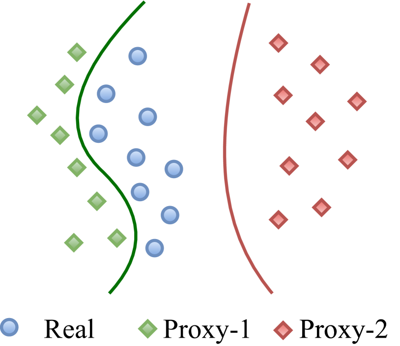
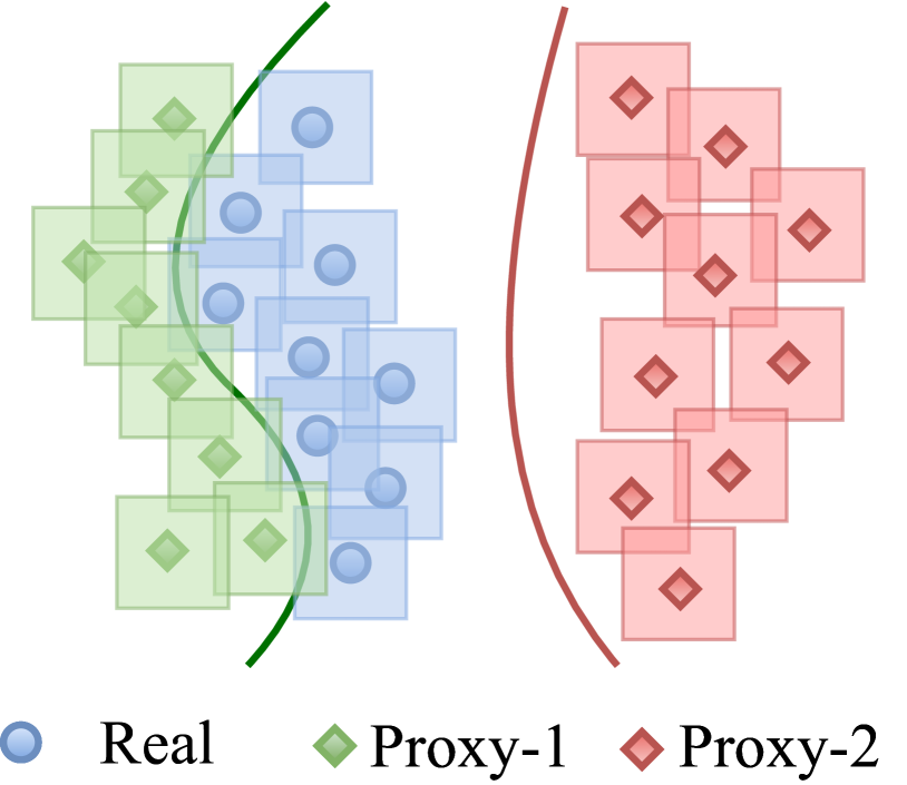
Robust discrimination. Our metric works based on how well a discriminator can robustly distinguish between samples from the real and proxy distributions. Compared to a typical discriminator, the robust discriminator should be accurate even when there is an adversary who can perturb the sampled instance by a perturbation of size . Intuitively, if there exists a successful and robust discriminator for two distributions and , then it means that no adversary can make instances of to look like instances of even by making perturbations of size . This means that and are far away from each other (Figure 1). On the other hand, if no robust discriminator exists, then it means that the adversary can ”align“ most of the mass of proxy distribution with that of real distribution by making perturbations of size at most . This notion is closely related to the optimal transport between the proxy and real distribution. In particular, the optimal adversary here corresponds to a transport that minimizes (Compare with Definition 2). To be more specific, the goal of a robust discriminator is to maximize its robust accuracy333All the definitions of accuracy and robust accuracy in this section are defined for true distributions. However, in the experiments we work with their empirical variant.:
We use to denote the accuracy of best existing robust discriminator, namely, . Note that as grows from to , the robust accuracy of any discriminator will decrease to at most . If two distributions and are close to each other, this drop in accuracy happens much faster since the adversary can make images from two distributions to look alike by adding smaller perturbations. We use this intuition and define our metric ARC as follows:
In other words, the ARC metric is equal to the area under the robust discrimination accuracy v.s. perturbation curve (See Figure 3 for a sample of this curve.) In Section 3.2, we discuss how this metric can be calculated with only samples from the real data and proxy distributions. When selecting a proxy distribution, we choose the one with the smallest ARC value, since it is expected to be closest to real data distribution. We also demonstrate that ARC metric is directly related to conditional Wasserstein distance. In particular, we have the following Theorem:
Theorem 2.
For any two distributions and with equal class probabilities we have . Moreover, if for all labels , and are two concentric uniform spheres, then we have .
Why non-robust discrimination is not an effective metric. Deep neural networks are commonly used as a discriminator between synthetic and real images (Goodfellow et al., 2014; Gui et al., 2020). In our experiments, we find that even a four-layer convolutional network can achieve near 100% classification accuracy on all selected proxy distributions (Appendix C.1). This result shows that non-robust discrimination is not an effective measure of proximity (as highlighted in Figure 1).
2.3 Bringing it all together: Improving adversarial robustness using proxy distributions
Overview of robust training. The key objective in robust training is to solve , where is determined by the training objective and is the threat model. In adversarial training (Madry et al., 2018; Zhang et al., 2019; Carmon et al., 2019; Pang et al., 2021), we train against projected gradient descent based (PGD) adversarial examples by selecting . In randomized smoothing (Cohen et al., 2019; Salman et al., 2019; Sehwag et al., 2020; Carmon et al., 2019), where the objective is to achieve certified robustness (Wong & Kolter, 2018), we aim to achieve invariance to random Gaussian Noise by selecting , where , and is the KL-divergence. This loss function (Zheng et al., 2016), referred to as robust stability training (RST), performs better than using (Carmon et al., 2019). We refer the in adversarial training and randomized smoothing as and , respectively. We represent the cross-entropy loss function, which is used to train the classifier, as , where and is the one-hot vector encoding of .
Our objective is to integrate synthetic samples from Proxy distributions in Robust Training (PORT). In particular, we use the following robust training formulation that combines samples from a real training dataset with synthetic samples.
where and is the aggregated adversarial loss over both and . Depending on training objective, we select either or as . We approximate the aggregated loss using available training samples from the real data distribution () and a set of synthetic images sampled from the proxy distribution (). We select through a hyperparameter search.
Which synthetic samples to choose? In particular, which set () of synthetic samples from the proxy distribution () leads to maximum transferred robustness on real data, i.e., , where is a robust learning algorithm. While it can be solved in many different ways, we follow a rejection sampling based approach. In particular, we measure proximity of each synthetic sample to real data distribution and use it as a metric to accept or reject a sample. We use output probability score from our trained robust discriminators as a measure of proximity. In particular we define as the final score for each synthetic sample, where samples with lowest score are prioritized in the selection.
3 Experimental results
First, we show that our proposed approach of using proxy distributions brings significant improvements in the performance of both adversarial training and randomized smoothing across both and threat models (Section 3.1). We also uncover that diffusion-based generative models are more effective proxy distributions than generative adversarial networks (GANs) on multiple datasets. Next we delve deeper into why diffusion-based generative models are highly effective proxy distributions (Section 3.2). We find that the key reason behind the success of diffusion based models is the that there is no robust discriminator that can robustly distinguish between the samples from diffusion based models and real data distribution. We demonstrate that our proposed metric (ARC) provides a better characterization of the effectiveness of diffusion-based models than other widely used metrics. Finally, we investigate the effectiveness of adaptively selecting synthetic images in our framework.
3.1 Improving robustness using synthetic images from proxy distributions
Setup. We consider five datasets, namely CIFAR-10 (Krizhevsky et al., 2014), CIFAR-100 (Krizhevsky et al., 2014), CelebA (Liu et al., 2015), AFHQ (Choi et al., 2020), and ImageNet (Deng et al., 2009). We also work with commonly used and threat models for adversarial attacks and use AutoAttack (Croce & Hein, 2020) to measure robustness. We provide extensive details on the setup in Appendix B.
Evaluation metrics for robust training. We use two key metrics to evaluate performance of trained models: clean accuracy and robust accuracy. While the former refers to the accuracy on unmodified test set images, the latter refers to the accuracy on adversarial examples generated from test set images. We refer to the robust accuracy of any discriminator trained to distinguish between synthetic and real data as robust discrimination accuracy. We also use randomized smoothing to measure certified robust accuracy, i.e., robust accuracy under strongest possible adversary in the threat model.
Synthetic data. We sample synthetic images from a generative models, in particular from denoising diffusion-based probabilistic models (DDPM) (Ho et al., 2020; Nichol & Dhariwal, 2021). We provide extensive details on the number of images sampled and the sampling procedure in Appendix B. We use as it achieves best results (Appendix D). We combine real and synthetic images in a : ratio in each batch, thus irrespective of the number of synthetic images, our training time is only twice of the baseline methods.
3.1.1 Improving performance of adversarial training
State-of-the-art robust accuracy synthetic images (Table 1, 2). Using synthetic images from diffusion-based generative models (DDPM), our approach achieves state-of-the-art robust accuracy in the category of not using any extra real world data (Croce et al., 2020). We improve robust accuracy by up to % and % over previous works in and threat model, respectively. Notably, the gain in performance is highest for the CIFAR-10 and Celeb-A datasets. Note that by using only synthetic images, our work also achieves competitive performance with previous works that use extra real-world images. For example, using additional real-data Carmon et al. (2019) achieve % robust accuracy on CIFAR-10 () while we achieve % robust accuracy by using only synthetic data.
| Clean | Auto | Clean | Auto | ||
|---|---|---|---|---|---|
| Baseline | |||||
| PORT | |||||
| Clean | Auto | Clean | Auto | ||
|---|---|---|---|---|---|
| Baseline | |||||
| PORT | |||||
| Clean | Auto | |
|---|---|---|
| Baseline | ||
| PORT | ||
Proxy distribution offsets increase in network parameters. We find that gains from using synthetic samples are equivalent to ones obtained by scaling network size by an order of magnitude (Table 1). For example, a ResNet-18 network with synthetic data achieves higher robust accuracy () than a Wrn-34-20 trained without it, while having fewer parameters than the latter. Similar trend holds for Wrn-34-10 networks, when compared with a much larger Wrn-70-16 network. This trend also holds for both and threat models.
Simultaneous improvement in clean accuracy. Due to the accuracy vs robustness trade-off in adversarial training, improvement in robust accuracy often comes at the cost of clean accuracy. However synthetic samples provide a boost in both clean and robust accuracy, simultaneously. Using adaptively sampled synthetic images, we observe improvement in clean accuracy by up to % and % across and threat models, respectively.
Comparison across generative models. We find that synthetic samples from diffusion-based generative models (Ho et al., 2020; Nichol & Dhariwal, 2021) provides significantly higher improvement in performance than generative adversarial networks (GANs) (Table 4). We further investigate this phenomenon in the next section.
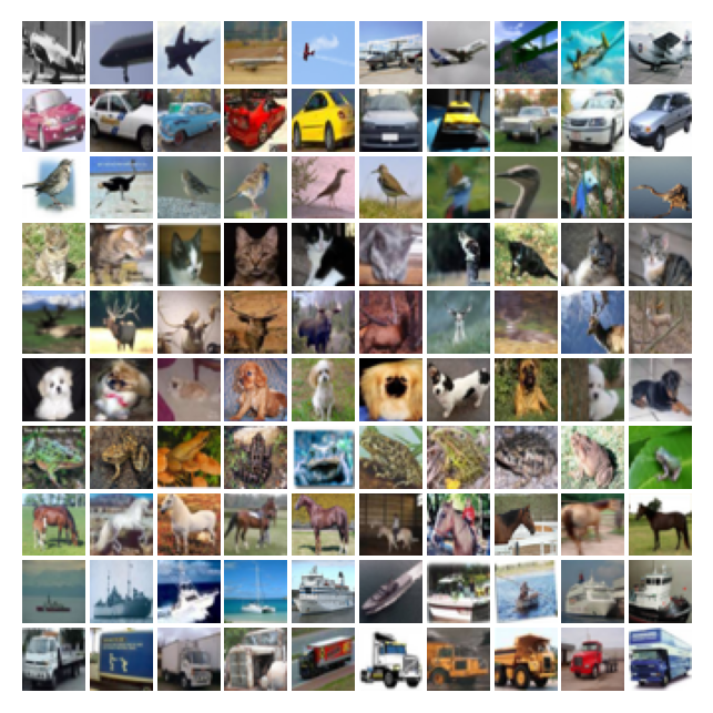
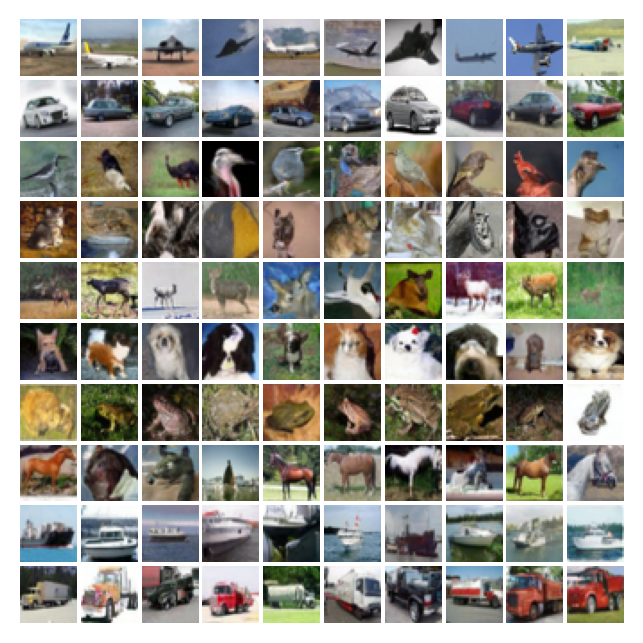
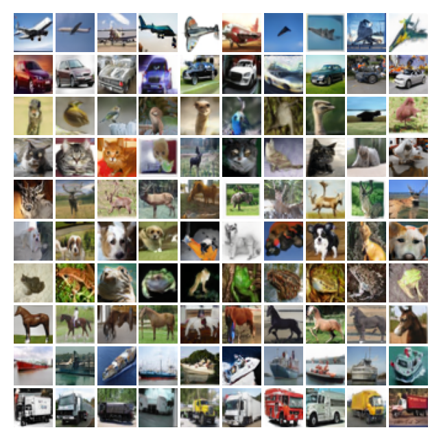
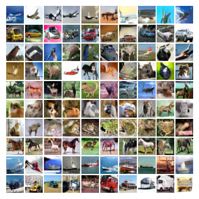
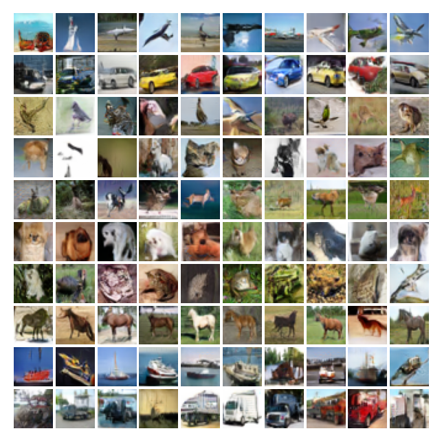
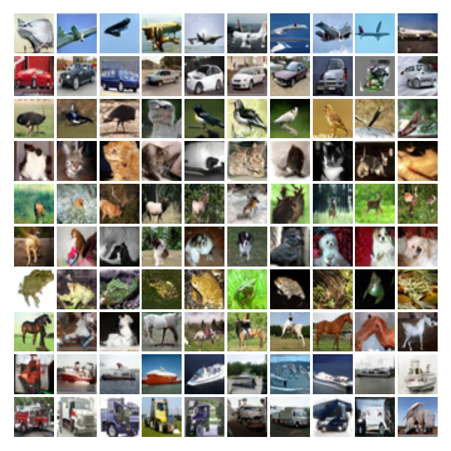
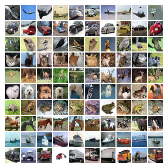
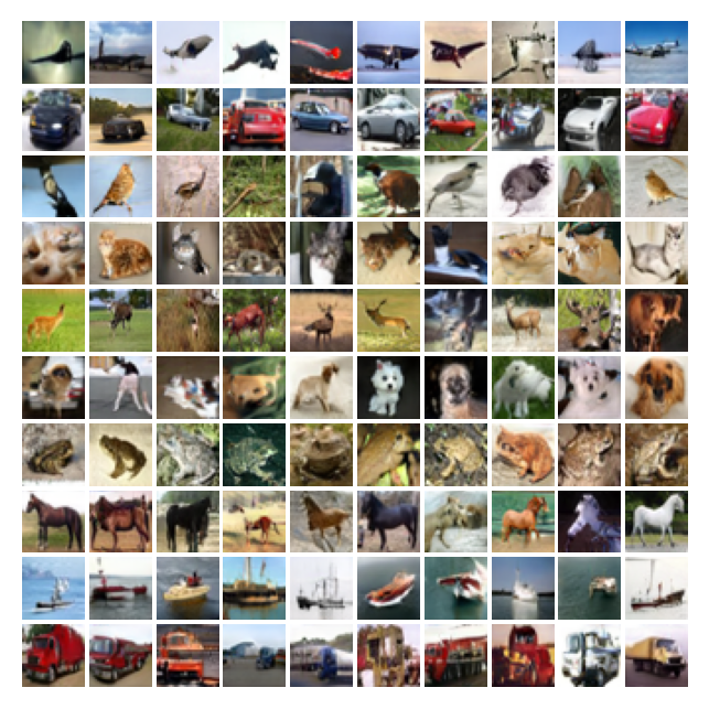
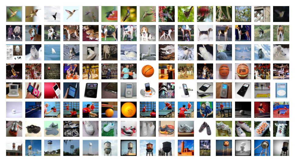
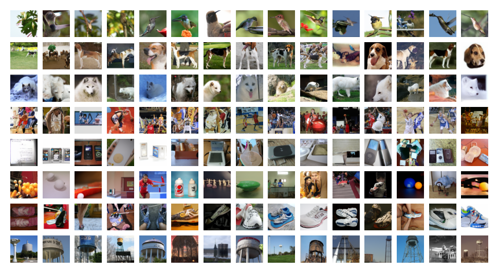
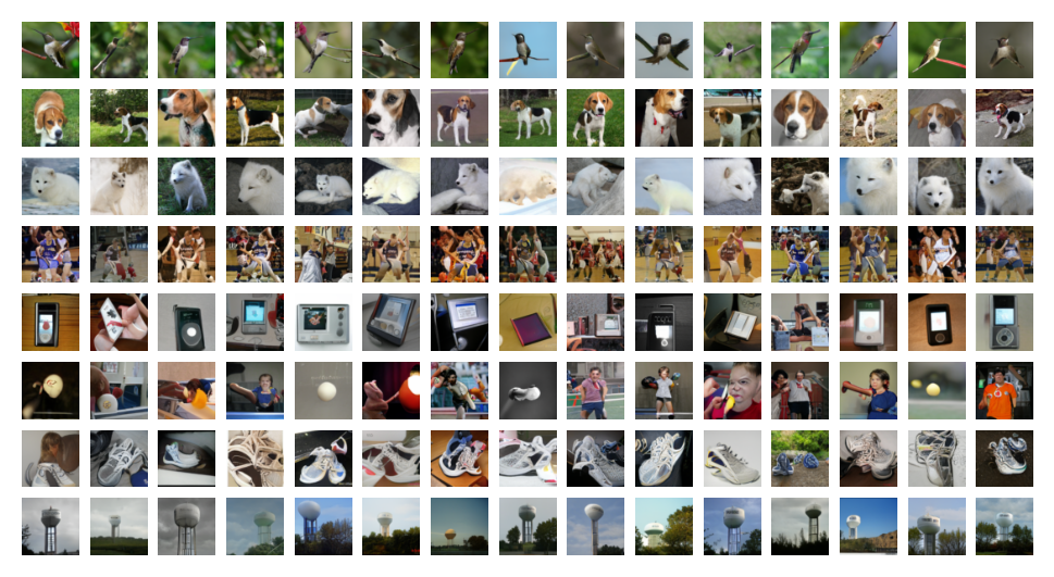
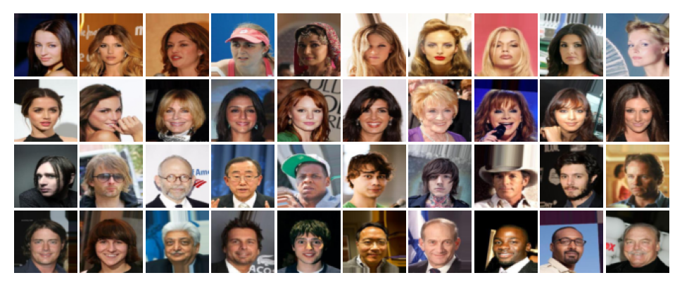
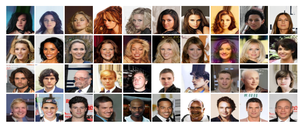
We further analyze sample complexity of adversarial training using synthetic data in Appendix D.1. We also provide visual examples of real and synthetic images for each dataset at the end of the paper.
| Dataset |
|
Clean | Auto | ||
|---|---|---|---|---|---|
| CIFAR-10 | None | ||||
| StyleGAN | |||||
| DDPM | |||||
| CelebA | None | ||||
| StyleFormer | |||||
| DDPM | |||||
| ImageNet | None | ||||
| BigGAN | |||||
| DDPM |
3.1.2 Improving certified robustness with randomized smoothing
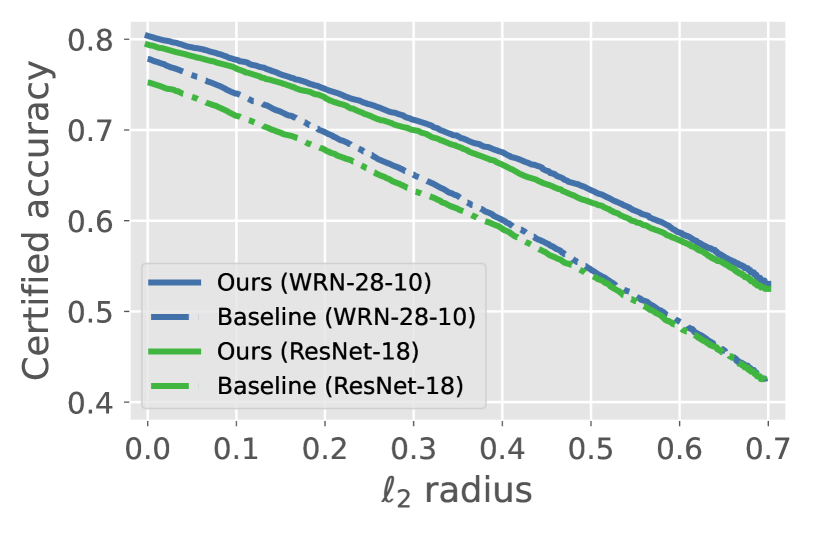
We provide results on certified adversarial robustness in Table 5. We first compare the performance of our proposed approach with the baseline technique, i.e., RST (Carmon et al., 2019). We achieve significantly higher certified robust accuracy than the baseline approach at all perturbations budgets for both ResNet-18 and Wrn-28-10 network architectures. Additionally, the robustness of our approach decays at a smaller rate than the baseline. At perturbation of , equivalent to perturbation of , our approach achieves % higher certified robust accuracy than RST. We also significantly outperform other certified robustness techniques which aren’t based on randomized smoothing (Zhang et al., 2020; Wong et al., 2018; Balunovic & Vechev, 2019). Along with better certified robust accuracy, our approach also achieves better clean accuracy than most previous approaches, simultaneously.
Synthetic images vs real-world images. Using only synthetic samples (M), we also outperform RST where it uses an additional curated set of K real-world images (RST500K). While the latter achieves % certified robust accuracy, we improve it to %.
3.2 Delving deeper into use of proxy distributions in robust training
Earlier in Section 3.1 we showed that diffusion-based generative models are an excellent choice for a proxy distribution for many datasets. Now we characterize the benefit of individual proxy distributions in our robust training framework. We consider seven different generative models, which are well-representative of the state-of-the-art on the CIFAR-10 dataset.
Using synthetic-to-real transfer of robustness as ground truth. From each generative model we sample one million synthetic images. We adversarially train a ResNet-18 (He et al., 2016) network on these images and rank generative models in order of robust accuracy achieved on the CIFAR-10 test set. We provide further experimental setup details in Appendix C.
Calculating ARC. At each perturbation budget (), we adversarially train a ResNet-18 classifier to distinguish between synthetic and real images. We measure robust discrimination accuracy of trained classifier on a balanced held-out validation set. We calculate ARC by measuring the area under the robust discrimination accuracy and perturbation budget curve444We use numpy.trapz(Racc-0.5, ) to calculate ARC. (Figure 3). We provide a detailed comparison of it with other metrics in Table 6.
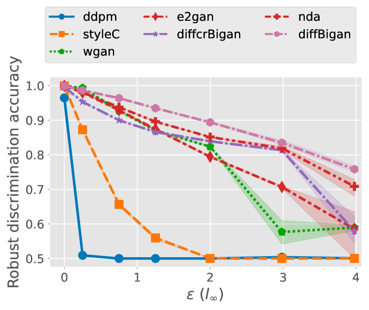
| Rank | Model |
|
|
IS () | 1-NN() | ARC () | |||
| – | CIFAR-10 555Using 50,000 training images from the CIFAR-10 dataset. | – | – | – | – | ||||
| DDPM (UC) 666UC and C refers to unconditional and conditional generative models, respectively. | (2) | (2) | (2) | (1) | |||||
| StyleGAN (C) | (1) | (1) | (3) | (2) | |||||
| WGAN-ALP (UC) | (7) | (7) | (7) | (3) | |||||
| E2GAN (UC) | (5) | (5) | (1) | (4) | |||||
| DiffCrBigGAN (C) | (3) | (3) | (6) | (5) | |||||
| NDA (C) | (6) | (6) | (5) | (6) | |||||
| DiffBigGAN (C) | (4) | (4) | (4) | (7) | |||||
| Mean absolute ranking difference | |||||||||
ARC is highly effective at determining synthetic to real transfer of robustness (Table 6). Each of the baseline metrics, including FID which is widely used, fail in accurately predicting the transfer of robustness from synthetic to real distributions. Even more, they also fail to identify DDPM (Ho et al., 2020) as the most successful proxy distribution. Our proposed metric (ARC), which measures the distinguishability of perturbed synthetic and real images, exactly predicts the ranking of different generative models in terms of the transfer of robustness. It also provides deeper insight into why synthetic samples from DDPM models are highly effective compared to other models. As shown in Figure 3, discrimination between DDPM samples and real images becomes almost impossible even at very small perturbations budgets. A more detailed comparison is provided in Appendix C.2.
Adaptive sampling of synthetic data based on ARC (Appendix C.3). We compare the benefit of adaptive sampling with random sampling on CIFAR-10 dataset (for both and threat models). Our adaptive sampling achieves an average of and improvement in robust accuracy over random sampling in the and threat models, respectively.
4 Related work
Transfer of adversarial robustness. This line of work focuses on the transfer of adversarial robustness, i.e., correct classification even under adversarial perturbations, when testing the model on different data distributions (Shafahi et al., 2020; Sehwag et al., 2019). Note that this is different from just achieving correct classification on unmodified images across different distributions (Taori et al., 2020; Hendrycks & Dietterich, 2019). Here we provide a theoretical analysis of the transfer of adversarial robustness between data distributions.
Using extra curated real-world data in robust training. Prior works (Zhai et al., 2019; Carmon et al., 2019; Uesato et al., 2019; Najafi et al., 2019; Deng et al., 2021) have argued for using more training data in adversarial training and often resort to curating additional real-world samples. In contrast, we model the proxy distribution from the limited training images available and sample additional synthetic images from this distribution.
Generative models for proxy distributions. State-of-the-art generative models are capable of modeling the distribution of current large-scale image datasets. In particular, generative adversarial networks (GANs) have excelled at this task (Goodfellow et al., 2014; Karras et al., 2020; Gui et al., 2020). Though GANs generate images with high fidelity, they often lack high diversity (Ravuri & Vinyals, 2019). However, samples from recently proposed diffusion process based models achieve both high diversity and fidelity (Ho et al., 2020; Nichol & Dhariwal, 2021). Fréchet Inception Distance (FID) (Heusel et al., 2017) and Inception Score (IS) (Heusel et al., 2017) are two common metrics to evaluate the quality of samples from generative models.
Using generative models to improve adversarial robustness. Earlier works have used generative models to learn training data manifold and the use it to map input samples to data manifold (Samangouei et al., 2018; Jalal et al., 2017; Xu et al., 2018). However, most of these techniques are broken against adaptive attacks (Athalye et al., 2018; Tramèr et al., 2020). We use generative models to sample additional training samples which further improve the adversarial robustness.
Comparison with Rebuffi et al. (2021). A concurrent work by Rebuffi et al. (2021) also uses randomly sampled synthetic images to improve adversarial robustness. In comparison, we provide a theoretical analysis of when synthetic data helps along with metrics to optimize the selection of both generative models and individual samples. We also demonstrate an improvement in certified robust accuracy using synthetic samples. Despite these differences, similar benefits of using proxy distributions in two independent and concurrent works further ascertain the importance of this research direction.
5 Discussion and Broader Outlook
Using synthetic data has been a compelling solution in many applications, such as healthcare (Jordon et al., 2018) and autonomous driving (Mayer et al., 2016) since it makes collecting a large amount of data feasible. In a similar spirit, we use synthetic data to make deep neural networks more robust against adversarial attacks. We investigate foundational questions such as determining the transfer of robustness from synthetic to real data and determining selection criteria for how to choose generative models or individual samples. Finally, we note that while it is crucial to improve robustness against the threat of adversarial examples, it also has an unwanted side-effect in domains where adversarial examples are used for good. Recent works use them to provide privacy on the web (Shan et al., 2020) or to evade website fingerprinting methods (Rahman et al., 2020). Improving defenses against adversarial examples will negatively hurt these applications.
6 Reproducibility
We provide proof of each of our theorems in Appendix A. Similarly, we provide extensive details on our experimental setup in Appendix B. Our work is also featured on RobustBench (Croce et al., 2020), an external benchmark for standardized evaluation of adversarial robustness. Our robustly trained models are also available through the RobustBench API. For further reproducibility, we have also submitted our code with the supplementary material.
References
- Athalye et al. (2018) Anish Athalye, Nicholas Carlini, and David Wagner. Obfuscated gradients give a false sense of security: Circumventing defenses to adversarial examples. In International Conference on Machine Learning, pp. 274–283. PMLR, 2018.
- Balunovic & Vechev (2019) Mislav Balunovic and Martin Vechev. Adversarial training and provable defenses: Bridging the gap. In International Conference on Learning Representations, 2019.
- Bhagoji et al. (2019) Arjun Nitin Bhagoji, Daniel Cullina, and Prateek Mittal. Lower bounds on adversarial robustness from optimal transport. In Advances in Neural Information Processing Systems, pp. 7496–7508, 2019.
- Biggio & Roli (2018) Battista Biggio and Fabio Roli. Wild patterns: Ten years after the rise of adversarial machine learning. volume 84, pp. 317–331. Elsevier, 2018.
- Biggio et al. (2013) Battista Biggio, Igino Corona, Davide Maiorca, Blaine Nelson, Nedim Šrndić, Pavel Laskov, Giorgio Giacinto, and Fabio Roli. Evasion attacks against machine learning at test time. In Joint European conference on machine learning and knowledge discovery in databases, pp. 387–402. Springer, 2013.
- Brock et al. (2019) Andrew Brock, Jeff Donahue, and Karen Simonyan. Large scale gan training for high fidelity natural image synthesis. In International Conference on Learning Representations, 2019.
- Carmon et al. (2019) Yair Carmon, Aditi Raghunathan, Ludwig Schmidt, John C Duchi, and Percy S Liang. Unlabeled data improves adversarial robustness. In Advances in Neural Information Processing Systems, pp. 11190–11201, 2019.
- Choi et al. (2020) Yunjey Choi, Youngjung Uh, Jaejun Yoo, and Jung-Woo Ha. Stargan v2: Diverse image synthesis for multiple domains. In Proceedings of the IEEE/CVF Conference on Computer Vision and Pattern Recognition, pp. 8188–8197, 2020.
- Cohen et al. (2019) Jeremy Cohen, Elan Rosenfeld, and Zico Kolter. Certified adversarial robustness via randomized smoothing. In International Conference on Machine Learning, pp. 1310–1320. PMLR, 2019.
- Croce & Hein (2020) Francesco Croce and Matthias Hein. Reliable evaluation of adversarial robustness with an ensemble of diverse parameter-free attacks. In International Conference on Machine Learning, pp. 2206–2216. PMLR, 2020.
- Croce et al. (2020) Francesco Croce, Maksym Andriushchenko, Vikash Sehwag, Nicolas Flammarion, Mung Chiang, Prateek Mittal, and Matthias Hein. Robustbench: a standardized adversarial robustness benchmark. arXiv preprint arXiv:2010.09670, 2020.
- Cui et al. (2021) Jiequan Cui, Shu Liu, Liwei Wang, and Jiaya Jia. Learnable boundary guided adversarial training. In Proceedings of the IEEE/CVF International Conference on Computer Vision, pp. 15721–15730, 2021.
- Cullina et al. (2018) Daniel Cullina, Arjun Nitin Bhagoji, and Prateek Mittal. Pac-learning in the presence of adversaries. volume 31, pp. 230–241, 2018.
- Deng et al. (2009) Jia Deng, Wei Dong, Richard Socher, Li-Jia Li, Kai Li, and Li Fei-Fei. Imagenet: A large-scale hierarchical image database. In 2009 IEEE conference on computer vision and pattern recognition, pp. 248–255. Ieee, 2009.
- Deng et al. (2021) Zhun Deng, Linjun Zhang, Amirata Ghorbani, and James Zou. Improving adversarial robustness via unlabeled out-of-domain data. In International Conference on Artificial Intelligence and Statistics, pp. 2845–2853. PMLR, 2021.
- Diochnos et al. (2018) Dimitrios I Diochnos, Saeed Mahloujifar, and Mohammad Mahmoody. Adversarial risk and robustness: general definitions and implications for the uniform distribution. In Proceedings of the 32nd International Conference on Neural Information Processing Systems, pp. 10380–10389, 2018.
- Dowson & Landau (1982) DC Dowson and BV Landau. The fréchet distance between multivariate normal distributions. In Journal of multivariate analysis, volume 12, pp. 450–455, 1982.
- Gilmer et al. (2018) Justin Gilmer, Luke Metz, Fartash Faghri, Samuel S Schoenholz, Maithra Raghu, Martin Wattenberg, and Ian Goodfellow. Adversarial spheres. arXiv preprint arXiv:1801.02774, 2018.
- Givens et al. (1984) Clark R Givens, Rae Michael Shortt, et al. A class of wasserstein metrics for probability distributions. In The Michigan Mathematical Journal, volume 31, pp. 231–240, 1984.
- Goodfellow et al. (2014) Ian Goodfellow, Jean Pouget-Abadie, Mehdi Mirza, Bing Xu, David Warde-Farley, Sherjil Ozair, Aaron Courville, and Yoshua Bengio. Generative adversarial nets. In Advances in Neural Information Processing Systems, volume 27, 2014.
- Gowal et al. (2020) Sven Gowal, Chongli Qin, Jonathan Uesato, Timothy Mann, and Pushmeet Kohli. Uncovering the limits of adversarial training against norm-bounded adversarial examples. arXiv preprint arXiv:2010.03593, 2020.
- Gui et al. (2020) Jie Gui, Zhenan Sun, Yonggang Wen, Dacheng Tao, and Jieping Ye. A review on generative adversarial networks: Algorithms, theory, and applications. arXiv preprint arXiv:2001.06937, 2020.
- He et al. (2016) Kaiming He, Xiangyu Zhang, Shaoqing Ren, and Jian Sun. Deep residual learning for image recognition. In Proceedings of the IEEE conference on computer vision and pattern recognition, pp. 770–778, 2016.
- Hendrycks & Dietterich (2019) Dan Hendrycks and Thomas G. Dietterich. Benchmarking neural network robustness to common corruptions and perturbations. In 7th International Conference on Learning Representations, 2019.
- Heusel et al. (2017) Martin Heusel, Hubert Ramsauer, Thomas Unterthiner, Bernhard Nessler, and Sepp Hochreiter. Gans trained by a two time-scale update rule converge to a local nash equilibrium. In Advances in neural information processing systems, volume 30, 2017.
- Ho et al. (2020) Jonathan Ho, Ajay Jain, and Pieter Abbeel. Denoising diffusion probabilistic models. In Advances in Neural Information Processing Systems, volume 33, pp. 6840–6851, 2020.
- Jalal et al. (2017) Ajil Jalal, Andrew Ilyas, Constantinos Daskalakis, and Alexandros G Dimakis. The robust manifold defense: Adversarial training using generative models. arXiv preprint arXiv:1712.09196, 2017.
- Jordon et al. (2018) James Jordon, Jinsung Yoon, and Mihaela Van Der Schaar. Pate-gan: Generating synthetic data with differential privacy guarantees. In International Conference on Learning Representations, 2018.
- Karras et al. (2020) Tero Karras, Miika Aittala, Janne Hellsten, Samuli Laine, Jaakko Lehtinen, and Timo Aila. Training generative adversarial networks with limited data. In Advances in Neural Information Processing Systems, volume 33, pp. 12104–12114, 2020.
- Kolesnikov et al. (2020) Alexander Kolesnikov, Lucas Beyer, Xiaohua Zhai, Joan Puigcerver, Jessica Yung, Sylvain Gelly, and Neil Houlsby. Big transfer (bit): General visual representation learning. In ECCV, 2020.
- Krizhevsky et al. (2014) Alex Krizhevsky, Vinod Nair, and Geoffrey Hinton. The cifar-10 dataset. online: http://www. cs. toronto. edu/kriz/cifar. html, 2014.
- LeCun & Cortes (2010) Yann LeCun and Corinna Cortes. MNIST handwritten digit database. AT&T Labs [Online]. Available: http://yann. lecun. com/exdb/mnist, 2010.
- Liu et al. (2015) Ziwei Liu, Ping Luo, Xiaogang Wang, and Xiaoou Tang. Deep learning face attributes in the wild. In Proceedings of the IEEE international conference on computer vision, pp. 3730–3738, 2015.
- Madry et al. (2018) Aleksander Madry, Aleksandar Makelov, Ludwig Schmidt, Dimitris Tsipras, and Adrian Vladu. Towards deep learning models resistant to adversarial attacks. International Conference on Learning Representations, 2018.
- Mahajan et al. (2018) Dhruv Mahajan, Ross Girshick, Vignesh Ramanathan, Kaiming He, Manohar Paluri, Yixuan Li, Ashwin Bharambe, and Laurens Van Der Maaten. Exploring the limits of weakly supervised pretraining. In Proceedings of the European Conference on Computer Vision (ECCV), pp. 181–196, 2018.
- Mahloujifar et al. (2019a) Saeed Mahloujifar, Dimitrios I Diochnos, and Mohammad Mahmoody. The curse of concentration in robust learning: Evasion and poisoning attacks from concentration of measure. In Proceedings of the AAAI Conference on Artificial Intelligence, volume 33, pp. 4536–4543, 2019a.
- Mahloujifar et al. (2019b) Saeed Mahloujifar, Xiao Zhang, Mohammad Mahmoody, and David Evans. Empirically measuring concentration: Fundamental limits on intrinsic robustness. arXiv preprint arXiv:1905.12202, 2019b.
- Mayer et al. (2016) Nikolaus Mayer, Eddy Ilg, Philip Hausser, Philipp Fischer, Daniel Cremers, Alexey Dosovitskiy, and Thomas Brox. A large dataset to train convolutional networks for disparity, optical flow, and scene flow estimation. In Proceedings of the IEEE conference on computer vision and pattern recognition, pp. 4040–4048, 2016.
- Montasser et al. (2019) Omar Montasser, Steve Hanneke, and Nathan Srebro. Vc classes are adversarially robustly learnable, but only improperly. In Conference on Learning Theory, pp. 2512–2530. PMLR, 2019.
- Najafi et al. (2019) Amir Najafi, Shin-ichi Maeda, Masanori Koyama, and Takeru Miyato. Robustness to adversarial perturbations in learning from incomplete data. In Proceedings of the 33rd International Conference on Neural Information Processing Systems, pp. 5541–5551, 2019.
- Nakkiran et al. (2021) Preetum Nakkiran, Behnam Neyshabur, and Hanie Sedghi. The bootstrap framework: Generalization through the lens of online optimization. In International Conference on Learning Representations, 2021.
- Nichol & Dhariwal (2021) Alexander Quinn Nichol and Prafulla Dhariwal. Improved denoising diffusion probabilistic models. In Proceedings of the 38th International Conference on Machine Learning, volume 139, pp. 8162–8171. PMLR, 2021.
- Pang et al. (2021) Tianyu Pang, Xiao Yang, Yinpeng Dong, Hang Su, and Jun Zhu. Bag of tricks for adversarial training. In International Conference on Learning Representations, 2021.
- Park & Kim (2021) Jeeseung Park and Younggeun Kim. Styleformer: Transformer based generative adversarial networks with style vector. arXiv preprint arXiv:2106.07023, 2021.
- Rade & Moosavi-Dezfooli (2021) Rahul Rade and Seyed-Mohsen Moosavi-Dezfooli. Helper-based adversarial training: Reducing excessive margin to achieve a better accuracy vs. robustness trade-off. In ICML 2021 Workshop on Adversarial Machine Learning, 2021.
- Rahman et al. (2020) Mohammad Saidur Rahman, Mohsen Imani, Nate Mathews, and Matthew Wright. Mockingbird: Defending against deep-learning-based website fingerprinting attacks with adversarial traces. volume 16, pp. 1594–1609. IEEE, 2020.
- Ravuri & Vinyals (2019) Suman Ravuri and Oriol Vinyals. Classification accuracy score for conditional generative models. In Advances in Neural Information Processing Systems, volume 32, 2019.
- Rebuffi et al. (2021) Sylvestre-Alvise Rebuffi, Sven Gowal, Dan A Calian, Florian Stimberg, Olivia Wiles, and Timothy Mann. Fixing data augmentation to improve adversarial robustness. arXiv preprint arXiv:2103.01946, 2021.
- Recht et al. (2019) Benjamin Recht, Rebecca Roelofs, Ludwig Schmidt, and Vaishaal Shankar. Do imagenet classifiers generalize to imagenet? In International Conference on Machine Learning, pp. 5389–5400. PMLR, 2019.
- Rice et al. (2020) Leslie Rice, Eric Wong, and Zico Kolter. Overfitting in adversarially robust deep learning. In International Conference on Machine Learning, pp. 8093–8104. PMLR, 2020.
- Salman et al. (2019) Hadi Salman, Jerry Li, Ilya P. Razenshteyn, Pengchuan Zhang, Huan Zhang, Sébastien Bubeck, and Greg Yang. Provably robust deep learning via adversarially trained smoothed classifiers. In 32 Annual Conference on Neural Information Processing Systems, pp. 11289–11300, 2019.
- Samangouei et al. (2018) Pouya Samangouei, Maya Kabkab, and Rama Chellappa. Defense-gan: Protecting classifiers against adversarial attacks using generative models. In International Conference on Learning Representations, 2018.
- Schmidt et al. (2018a) Ludwig Schmidt, Shibani Santurkar, Dimitris Tsipras, Kunal Talwar, and Aleksander Madry. Adversarially robust generalization requires more data. In Advances in Neural Information Processing Systems, volume 31, 2018a.
- Schmidt et al. (2018b) Ludwig Schmidt, Shibani Santurkar, Dimitris Tsipras, Kunal Talwar, and Aleksander Madry. Adversarially robust generalization requires more data. arXiv preprint arXiv:1804.11285, 2018b.
- Sehwag et al. (2019) Vikash Sehwag, Arjun Nitin Bhagoji, Liwei Song, Chawin Sitawarin, Daniel Cullina, Mung Chiang, and Prateek Mittal. Analyzing the robustness of open-world machine learning. In Proceedings of the 12th ACM Workshop on Artificial Intelligence and Security, pp. 105–116, 2019.
- Sehwag et al. (2020) Vikash Sehwag, Shiqi Wang, Prateek Mittal, and Suman Jana. Hydra: Pruning adversarially robust neural networks. In Advances in Neural Information Processing Systems, volume 33, pp. 19655–19666, 2020.
- Shafahi et al. (2019) Ali Shafahi, Mahyar Najibi, Mohammad Amin Ghiasi, Zheng Xu, John Dickerson, Christoph Studer, Larry S Davis, Gavin Taylor, and Tom Goldstein. Adversarial training for free! In Advances in Neural Information Processing Systems, 2019.
- Shafahi et al. (2020) Ali Shafahi, Parsa Saadatpanah, Chen Zhu, Amin Ghiasi, Christoph Studer, David W. Jacobs, and Tom Goldstein. Adversarially robust transfer learning. In 8th International Conference on Learning Representations, 2020.
- Shan et al. (2020) Shawn Shan, Emily Wenger, Jiayun Zhang, Huiying Li, Haitao Zheng, and Ben Y Zhao. Fawkes: Protecting privacy against unauthorized deep learning models. In 29th USENIX Security Symposium, pp. 1589–1604, 2020.
- Sinha et al. (2021) Abhishek Sinha, Kumar Ayush, Jiaming Song, Burak Uzkent, Hongxia Jin, and Stefano Ermon. Negative data augmentation. In International Conference on Learning Representations, 2021.
- Song et al. (2020) Jiaming Song, Chenlin Meng, and Stefano Ermon. Denoising diffusion implicit models. In International Conference on Learning Representations, 2020.
- Sun et al. (2017) Chen Sun, Abhinav Shrivastava, Saurabh Singh, and Abhinav Gupta. Revisiting unreasonable effectiveness of data in deep learning era. In Proceedings of the IEEE international conference on computer vision, pp. 843–852, 2017.
- Szegedy et al. (2014) Christian Szegedy, Wojciech Zaremba, Ilya Sutskever, Joan Bruna, Dumitru Erhan, Ian J. Goodfellow, and Rob Fergus. Intriguing properties of neural networks. In 2nd International Conference on Learning Representations, 2014.
- Taori et al. (2020) Rohan Taori, Achal Dave, Vaishaal Shankar, Nicholas Carlini, Benjamin Recht, and Ludwig Schmidt. Measuring robustness to natural distribution shifts in image classification. In Advances in Neural Information Processing Systems, volume 33, pp. 18583–18599, 2020.
- Terjék (2019) Dávid Terjék. Adversarial lipschitz regularization. In International Conference on Learning Representations, 2019.
- Tian et al. (2020) Yuan Tian, Qin Wang, Zhiwu Huang, Wen Li, Dengxin Dai, Minghao Yang, Jun Wang, and Olga Fink. Off-policy reinforcement learning for efficient and effective gan architecture search. In European Conference on Computer Vision, pp. 175–192. Springer, 2020.
- Torralba & Efros (2011) Antonio Torralba and Alexei A Efros. Unbiased look at dataset bias. In Conference on Computer Vision and Pattern Recognition (CVPR), pp. 1521–1528. IEEE, 2011.
- Tramèr et al. (2020) Florian Tramèr, Nicholas Carlini, Wieland Brendel, and Aleksander Madry. On adaptive attacks to adversarial example defenses. In 33 Annual Conference on Neural Information Processing Systems, 2020.
- Uesato et al. (2019) Jonathan Uesato, Jean-Baptiste Alayrac, Po-Sen Huang, Alhussein Fawzi, Robert Stanforth, and Pushmeet Kohli. Are labels required for improving adversarial robustness? In Advances in Neural Information Processing Systems, volume 32, 2019.
- Wang et al. (2019) Linnan Wang, Saining Xie, Teng Li, Rodrigo Fonseca, and Yuandong Tian. Sample-efficient neural architecture search by learning action space. arXiv preprint arXiv:1906.06832, 2019.
- Wong & Kolter (2018) Eric Wong and Zico Kolter. Provable defenses against adversarial examples via the convex outer adversarial polytope. In International Conference on Machine Learning, pp. 5286–5295. PMLR, 2018.
- Wong et al. (2018) Eric Wong, Frank R. Schmidt, Jan Hendrik Metzen, and J. Zico Kolter. Scaling provable adversarial defenses. In 31 Annual Conference on Neural Information Processing Systems, pp. 8410–8419, 2018.
- Wu et al. (2020a) Dongxian Wu, Shu-Tao Xia, and Yisen Wang. Adversarial weight perturbation helps robust generalization. Advances in Neural Information Processing Systems, 33, 2020a.
- Wu et al. (2020b) Dongxian Wu, Shu-Tao Xia, and Yisen Wang. Adversarial weight perturbation helps robust generalization. volume 33, 2020b.
- Xu et al. (2018) Weilin Xu, David Evans, and Yanjun Qi. Feature squeezing: Detecting adversarial examples in deep neural networks. In 25th Annual Network and Distributed System Security Symposium, 2018.
- Zagoruyko & Komodakis (2016) Sergey Zagoruyko and Nikos Komodakis. Wide Residual Networks. In British Machine Vision Conference, 2016.
- Zhai et al. (2019) Runtian Zhai, Tianle Cai, Di He, Chen Dan, Kun He, John Hopcroft, and Liwei Wang. Adversarially robust generalization just requires more unlabeled data. arXiv preprint arXiv:1906.00555, 2019.
- Zhang et al. (2019) Hongyang Zhang, Yaodong Yu, Jiantao Jiao, Eric Xing, Laurent El Ghaoui, and Michael Jordan. Theoretically principled trade-off between robustness and accuracy. In International Conference on Machine Learning, pp. 7472–7482, 2019.
- Zhang et al. (2020) Huan Zhang, Hongge Chen, Chaowei Xiao, Sven Gowal, Robert Stanforth, Bo Li, Duane S. Boning, and Cho-Jui Hsieh. Towards stable and efficient training of verifiably robust neural networks. In 8th International Conference on Learning Representations, 2020.
- Zhao et al. (2020) Shengyu Zhao, Zhijian Liu, Ji Lin, Jun-Yan Zhu, and Song Han. Differentiable augmentation for data-efficient gan training. Advances in Neural Information Processing Systems, 33, 2020.
- Zhao et al. (2020) Shuai Zhao, Liguang Zhou, Wenxiao Wang, Deng Cai, Tin Lun Lam, and Yangsheng Xu. Towards Better Accuracy-efficiency Trade-offs: Divide and Co-training. arXiv preprint arXiv:2011.14660, 2020.
- Zheng et al. (2016) Stephan Zheng, Yang Song, Thomas Leung, and Ian Goodfellow. Improving the robustness of deep neural networks via stability training. In Proceedings of the IEEE conference on computer vision and pattern recognition, pp. 4480–4488, 2016.
Appendix A Theoretical results
In this Section, we first provide the proofs of Theorem 1 and 2. Then we provide some additional results showing the tightness of our Theorem 1 and also the effect of combining real and proxy data on our Theorem. Finally, we provide some experimental result that validate our theory.
A.1 Proof of Theorem 1
Theorem 1:
Let and be two labeled distributions supported on with identical label distributions, i.e., . Then for any classifier
Sketch of the proof.
We first provide an informal sketch of the proof and then formalize the steps after that. Consider to be the distribution that is the outcome of the following process: First sample from , then find the closest such that and output 777Here, we assume that the closest point exists. Otherwise, We can set so that the distance is arbitrarily close to the infimum and the proof follows.. Also consider a similar distribution corresponding to . We now prove a Lemma that shows the conditional Wasserestein distance between and is equal to .
Lemma 3.
We have and .
Proof.
Let be the optimal transport between and . Also let be the joint distribution that is obtained by first sampling from and then setting . The marginals of are equal to and . Hence, is a valid transport between and . Also, define a potentially randomized perturbation algorithm that given an input samples , conditioned on and outputs . We have
On the other hand, because for all we have then . Therefore we have
Therefore we have
| (1) |
On the other hand, because is the optimal transport, we have
| (2) |
By the way the distributions and are defined we have
| (3) |
Roughly, the reason behind this is that all examples sampled from could be seen as an adversarial example for all elements of with the label . And we know that consists of optimal adversarial examples for , therefore, the optimal transport between and should be smaller than the optimal transport between and . Also, by triangle inequality for Wasserestein distance we have,
| (4) |
Full proof.
The following is a succinct formalization of the proof steps mentioned above, let be the optimal transport between the conditional distributions and . We have
With a similar argument we get and the proof is complete. ∎
A.2 Proof of Theorem 2
Theorem 2.
For any two distributions and with equal class probabilities we have . Moreover, if for all labels , and are two concentric uniform spheres, then we have .888The statement of theorem in the main body has a typographical error that is fixed here.
Proof.
We start by proving a lemma.
Lemma 4.
Let be an arbitrary transport between and . Then, for any discriminator we have,
Proof.
Consider an adversary that on input sampled from , samples a pair from the transport and return a center point between and such that if . Otherwise, it returns . Also, on a in input sampled from it samples a pair from the transport and return a center point between and such that if . Otherwise, it returns .
Denote to be the push-forward of under . And also denote . Now we have, where is the total variational distance. Therefore, no discriminator can distinguish from with accuracy more than . ∎
Now, let be a transport between and where is the optimal transport between and and is the probability of class for and . using Lemma 4 we have
Therefore we have
| (8) |
Now, by integration by parts we have
Therefore, we have
Now to prove the second part of theorem about the case of concentric spheres we start by following lemma.
Lemma 5.
Let and . Assume and are two concentric spheres according to the some norm. Also let be the optimal transport between and with respect to the same norm. Then we have,
Proof.
let be the uniform sphere centered at point and with radius and let be the uniform sphere centered at point and with radios . Observe that the optimal robust distinguisher for any is the one that assigns to if and assigns otherwise and for any we have
| (9) |
On the other hand, for any we have
| (10) |
Now consider optimal transport between and . Observe that this transport is equivalent to the following distribution:
Therefore, we have Which implies for any we have
| (11) |
and for any
| (12) |
Putting Equations equation 9, equation 10, equation 11, and equation 12 together, we finish the proof of Lemma. ∎
Having Lemma 5, we can follow the same steps as before except that instead of Inequality equation 8 we have an equality of the following form.
∎
A.3 Effect of Combining Proxy and Real Data on Theorem 1
A natural question is what happens when we combine the original distribution with the proxy distribution. For example, one might have access to a generative model but they want to combine the samples from the generative model with some samples from the original distribution and train a robust classifier on the aggregated dataset. The following corollary answers this question.
Theorem 6.
Let and be two labeled distributions supported on with identical label distributions and let be the weighted mixture of and . Then for any classifier
Note that the value of is usually very small as the number of data from proxy distribution is usually much higher than the original distribution. This shows that including (or not including) the data from original distribution should not have a large effect on the obtained bound on distribution-shift penalty.
Proof of Theorem 6.
We just need to show that Note that since the label distributions are equal, we have
Now let be the optimal transport between and . Now construct a joint distribution . Notice that is a joint distribution with marginals equal to and . Therefor is a transport between and and we can calculate its cost. We have
Therefore, we have
∎
A.4 Tightness of Theorem 1
Here, we show a theorem that shows our bound on distribution-shift penalty is tight. The following theorem shows that one cannot obtain a bound on the distribution-shift penalty for a specific classifier that is always better than our bound.
Theorem 7 (Tightness of Theorem 1).
For any distribution supported on , any classifier , any homogeneous distance and any , there is a labeled distribution such that
Proof.
for let be the distribution of the following process: First sample from , then find the closest such that and output . By definition, the conditional Wasserestein distance between and is equal to . We also have .
Observe that for any classifier we have because if is an adversarial example for , then is also an adversarial example for with distance . On the other hand we have because any adversarial example for with distance is also an adversarial example for with distance at most and since is the optimal adversarial example for then must be at least . Therefore, we have Putting everything together and setting we have
∎
Note that Theorem 7 only shows the tightness of Theorem 1 for a specific classifier. But there might exist a learning algorithm that incurs a much better bound in the expectation. Namely, there might exist such that for any two distributions and we have
We leave finding such an algorithm as an open question.
A.5 Experimental validation of main theorem
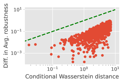
In theorem 1 we prove that transfer of adversarial robustness between two distributions is upper bounded by their conditional Wasserstein distance. Now we provide empirical validation of this result. We consider a -class classification problem where each class is modeled using a -dimensional multivariate normal distribution. In contrast to real-world datasets, where the underlying distribution of the data is unknown, we can efficiently and exactly calculate Wasserstein distance on this synthetic dataset. We robustly train a four-layer convolutional network on it. To construct a proxy distribution, we perturb both mean and covariance parameters across each class. On each proxy distribution, we measure the average robustness of the pre-trained model and its conditional Wasserstein distance from the original distribution. We use Wasserstein-2 distance999The bound in our theorem is based on . Since we know , using provides a loose upper bound., which has a closed-form expression for normal distributions (Givens et al., 1984). As shown in Figure 4, the difference in average robustness is upped bounded by the conditional Wasserstein distance.
Appendix B Additional details on experimental setup
We describe experimental details common across most experiments in this section. We discuss design choices pertaining to individual experiments in their respective sections.
Training setup. We use network architectures from the ResNet family, namely ResNet-18 (He et al., 2016) and variants of WideResNet (Zagoruyko & Komodakis, 2016). We train each network using stochastic gradient descent and learning rate with cosine learning rate decay, weight decay of , batch size , and epochs. We use weight decay on CIFAR-100 dataset, since higher weight decay further reduces the generalization gap on this dataset. We work with five datasets, namely CIFAR-10, CIFAR-100, ImageNet ( size images), CelebA (), and AFHQ (). For CelebA (Liu et al., 2015) dataset, we consider a four-class classification problem based on the attribute smile and male, i.e., smile/male, smile/not-male, not-smile/male, not-smile/not-male (total K images). Animal Faces-High-Quality (AFHQ) dataset comprises K images for three classes: cat, dog, and wild animals. Thus we consider the task of three-class classification on this dataset. To reduce the computational cost on ImageNet dataset, we use the free adversarial training (Shafahi et al., 2019) procedure. We use the ResNet-18 model for CIFAR-10, ImageNet, CelebA, and AFHQ dataset. However, for CIFAR-10 and CIFAR-100 dataset, we also use much larger Wrn-34-10 network.
Robust training parameters. We consider both and threat models. For CIFAR-10 and CIFAR-100 dataset, we use the commonly used perturbation budget () of and for and threat model, respectively. For other three dataset too, we choose commonly used perturbation budgets. We perform adversarial training using a 10-step projected gradient descent attack (PGD-10) and benchmark test set robustness with the much stronger AutoAttack101010We don’t report numbers with PGD attacks as AutoAttack already captures them while also making it easier to compare with other works (Croce et al., 2020). (Croce & Hein, 2020). We use , , samples for selection, and samples for estimation in randomized smoothing, as described in Cohen et al. (2019).
Generative models. We consider seven different generative models for the CIFAR-10 and two different networks for the CelebA and ImageNet dataset. In Table 7. We provide the number of synthetic images generated from each model and whether the generated images are labelled or unlabeled. If the model is unconditional, i.e., only generates unlabeled images, we label the images using an additional classifier. We use state-of-the-art LaNet (Wang et al., 2019) network to label images for the CIFAR-10 dataset. LaNet network is trained only on the training images of the CIFAR-10 dataset and achieves 99.0% accuracy on its test set. For CelebA dataset, we train a ResNet50 model to label synthetic images. For adaptive sampling of synthetic images for CIFAR-10 dataset, we first sample of set of M111111We use the M randomly sampled images made available by Nakkiran et al. (2021) along with M more sampled by us using improved sampling techniques (Nichol & Dhariwal, 2021) from the DDPM model. synthetic images from the DDPM model. Next we select M synthetic images with the lowest synthetic score from this set.
| Dataset |
|
Generative model |
|
Class-conditioned | ||||
| CIFAR-10 | K | DDPM Ho et al. (2020) | M | |||||
| StyleGAN (Karras et al., 2020) | M | |||||||
| WGAN-ALP (Terjék, 2019) | M | |||||||
| E2GAN (Tian et al., 2020) | M | |||||||
| DiffCrBigGAN (Zhao et al., 2020) | M | |||||||
| NDA (Sinha et al., 2021) | M | |||||||
| DiffBigGAN (Zhao et al., 2020) | M | |||||||
| CelebA | K | StyleFormer (Park & Kim, 2021) | M | |||||
| DDPM (Song et al., 2020) | 1M | |||||||
| ImageNet | M | BigGAN (Brock et al., 2019) | M | |||||
| DDPM (Nichol & Dhariwal, 2021) | K | |||||||
| CIFAR-100 | K | DDPM (Nichol & Dhariwal, 2021) | 1M | |||||
| AFHQ | K | StyleGAN (Karras et al., 2020) | K |
Evaluation metrics for generative models. We use following existing baseline metrics to evaluate the quality of synthetic samples. 1) Fréchet Inception Distance (FID): It measures the Fréchet distance (Dowson & Landau, 1982) between features of synthetic and real images extracted from an Inception-V3 network. 2) Inception score (IS): Unlike FID, Inception score only uses synthetic data with the goal to account for both fidelity and diversity of synthetic data. 3) Nearest neighbour distance (1-NN): It computes the average distance of a synthetic image to the nearest real image in the pixel space. 4) ARC: This is the metric we propose and it measures distance between synthetic and real data based on the success of a robust discriminator. We compare performance of all three baselines with our proposed metric.
Computational cost. In addition to robust training, sampling from generative models is another key contributor to the computational cost in our approach. We sample images from the DDPM model using steps for both CIFAR-10 and ImageNet datasets. Using an RTX 4x2080Ti GPU cluster, it takes hours to sample one million images on the CIFAR-10 dataset. With the same setup, it takes hours to sample K images for the ImageNet dataset. On both models, we use the publicly available checkpoints of pretrained generative models121212https://github.com/openai/improved-diffusion. Note that both training generative models and sampling from them is a one-time cost. Once the pretrained checkpoints and synthetic images are made publicly available, they can be directly used in downstream tasks. We will make our code and synthetic data publicly available.
| Clean | Auto | Clean | Auto | Clean | Auto | Clean | Auto | ||||
|---|---|---|---|---|---|---|---|---|---|---|---|
| Baseline | |||||||||||
| PORT | |||||||||||
Appendix C Delving deeper into robust discrimination and ARC
We propose a new metric (ARC), to rank different generative models in order of robustness transfer from their samples to real data. Now we provide experimental details on how we measure ARC and its comparison with other baselines.
Setup. A critical component in our approach is training a robust binary discriminator to distinguish between real and synthetic data. We use a ResNet-18 network for this task and train it for epochs with a learning rate, batch size, and 1e-4 weight decay. We use a randomly sampled set of one million images from each generative model. We keep synthetic images from this set for validation and train on the rest of them. We specifically choose images as it’s equal to the number of test images available in the CIFAR-10 test set, thus balancing both classes in our test set. We train for only steps per epoch, i.e., equivalent to a single pass through training images in the CIFAR-10 dataset. Thus over epochs, we effectively end up taking five passes through the one million synthetic images. Given the randomness in multiple steps, we aggregate results over three different runs of our experiments.
C.1 Why non-robust discriminators are not effective in measuring proximity?
We argue that most synthetic samples can be easily distinguished from real data, irrespective of proximity, in absence of adversarial perturbations (). This is likely because deep neural networks have very high expressive power. So a natural question is whether shallow networks, which have much lower capacity, are more suitable for this task. We test this hypothesis by using a two-layer (16 and 32 filters) and a four-layer (16, 16, 32, and 32 filters) convolutional neural network. We refer to them as CNN-2 and CNN-4, respectively. We find that even these shallow networks achieve more than % accuracy in distinguishing synthetic images from real images (Table 9). The CNN-4 network itself is achieving more than % accuracy for four out of seven generative models. A much larger ResNet-18 network achieves near-perfect classification accuracy for most models. Such high success of even shallow networks uniformly across generative models shows that non-robust discrimination is not an effective measure of proximity.
| Model | DDPM | StyleGAN | WGAN-ALP | E2GAN | DiffCrBigGAN | NDA | DiffBigGAN |
|---|---|---|---|---|---|---|---|
| CNN-2 | |||||||
| CNN-4 | |||||||
| ResNet-18 |
C.2 On effectiveness of ARC in measuring proximity
In this section, we delve deeper into the comparison of our proposed metric (ARC) with other baselines. We judge the success of each metric by how successfully it predicts the transfer of robustness from synthetic to real samples on the CIFAR-10 data. (referred to as transferred robust accuracy). We report our results in Table 10.
Is FID in CIFAR-10 feature space effective? When calculating FID, the recommended approach is to measure it in the feature space of a network trained on the ImageNet dataset (Heusel et al., 2017). One may ask, whether the reason behind the failure is using ImageNet feature space for CIFAR-10 images. This might be true as it is well known that most image datasets have their specific bias (Torralba & Efros, 2011). To answer this question, we measure FID in the feature of a state-of-the-art LaNet (Wang et al., 2019) networks trained on the CIFAR-10 dataset. We refer to this metric as FID (CIFAR-10). Similar to FID in ImageNet feature space, FID in CIFAR-10 feature space also fails to predict robustness transfer. It follows a similar trend as the former, where it ranks models like DiffBigGAN and StyleGAN much higher than other models.
Generalizing to natural training. If the objective is to maximize clean accuracy instead of robustness, one may ask whether ARC will remain effective in selecting the generative model. We answer this question by measuring the success of ARC in predicting how much clean accuracy is achieved on the CIFAR-10 test set when we train a ResNet-18 network only on one million synthetic images without any adversarial perturbation. Note that ARC is dependent only on samples, thus can be directly used for this task. We find that ARC correctly ranks DDPM over StyleGAN model for transferred clean accuracy. Similarly, it also correctly rank WGAN-ALP and E2GAN model higher than other BigGAN models where the former achieves higher clean accuracy on the CIFAR-10 test set. However, there are small variations in transferred clean accuracy with some models, such as WGAN-ALP and E2GAN, which ARC doesn’t capture in its ranking.
| Rank | Model |
|
|
|
|
IS () | 1-NN() | ARC () | ||||||||
|---|---|---|---|---|---|---|---|---|---|---|---|---|---|---|---|---|
| DDPM (UC) | ||||||||||||||||
| StyleGAN (C) | ||||||||||||||||
| WGAN-ALP (UC) | ||||||||||||||||
| E2GAN (UC) | ||||||||||||||||
| DiffCrBigGAN (C) | ||||||||||||||||
| NDA (C) | ||||||||||||||||
| DiffBigGAN (C) |
C.3 Adaptive sampling of synthetic data.
Finding synthetic samples which leads to highest synthetic-to-real robustness transfer. We use proximity of a synthetic sample to the original distribution, which we measure using synthetic score from our trained robust discriminators (using size perturbations), as a metric to judge transfer of performance from the proxy distribution to original distribution.
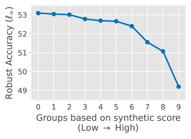
We sort the synthetic score for each of M synthetic images from the DDPM model and combine them into ten equal-size groups. Next, we adversarially train a ResNet-18 network on images from each group, along with CIFAR-10 training images, and measure robustness achieved on the CIFAR-10 test set (Figure 5). Our results validate the effectiveness of synthetic scores, where groups with the lowest synthetic score achieve highest robust test accuracy. The difference in the robust test accuracy is up to % between the group with the lowest score and the one with the highest score.
Improvement in performance with adaptive sampling. We select of set of M synthetic images (from a set of M) with the lowest synthetic score. We compare the success of these adaptively selected images with a set of M randomly selected images. We present our results in Table 11. It shows that adaptively sampling further improves the performance of our framework (PORT) across threat models ( and ) and network architectures.
Appendix D Bringing it all together: Using synthetic samples in robust training
In this section, we first analyze the synthetic images and later provide additional analysis based on them in robust training. We will primarily use synthetic images sampled from the DDPM and StyleGAN model.
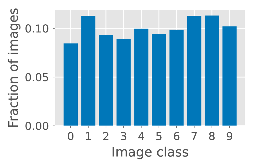
Analyzing synthetic images. Since DDPM is an unconditional model, it only generates unlabelled synthetic images. We label these images using a LaNet network on the CIFAR-10 dataset. We visualize the frequency of different classes in Figure 7. It shows that the synthetic images are almost uniformly distributed across classes. On the ImageNet dataset, we use the classifier conditioned sampling to generate labeled images from the improved DDPM model (Nichol & Dhariwal, 2021). We also provide samples images from different generative models in Figure 11 and 12.
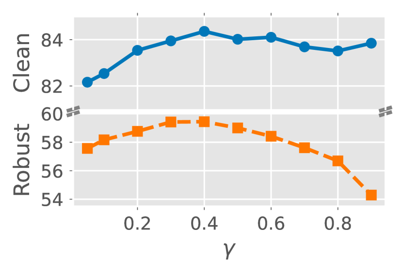
Hyperparameter search for . Before using DDPM images in robust training, we perform a hyperparameter search for . We consider ten different values from 0 to 1 and train a ResNet-18 network using PORT at each of them. We measure both the clean accuracy and robust accuracy of each network (Figure 7). We find that achieves the highest clean and robust accuracy. Thus we used in our experiments.
| Clean Accuracy | |||||
|---|---|---|---|---|---|
| Robust Accuracy |
D.1 Sample complexity of adversarial training
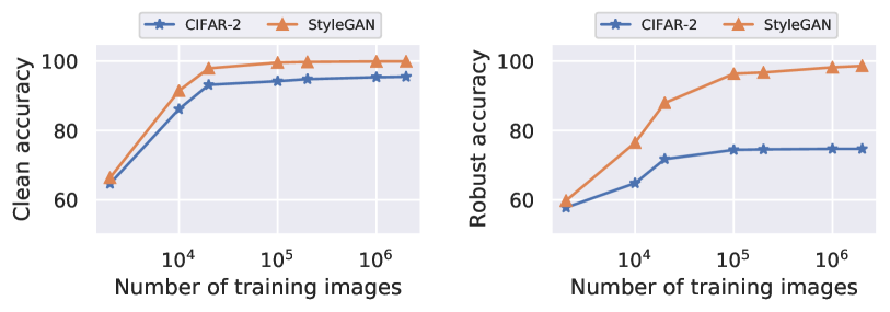
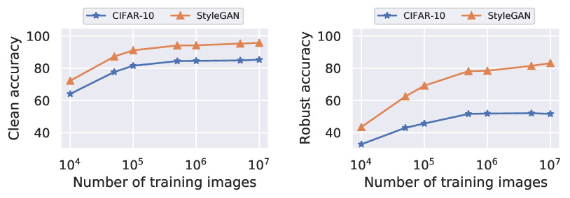
Given the ability to sample an unlimited amount of synthetic images from a proxy distribution, now we investigate the performance of adversarial training with an increasing number of training samples. We train the network only on synthetic images and measure its performance on another held-out set of synthetic images. We also measure how much the clean and robust accuracy transfers on the CIFAR-10 test set.
Setup. We primarily work with the CIFAR-10 dataset and its two-class subset, i.e., an easier problem of binary classification between class-1 (automobile) and class-9 (truck). We refer to the latter as CIFAR-2. We robustly train a ResNet-18 network on K to M synthetic images from the StyleGAN model, as in both -class and -class setup. We opt for StyleGAN over DDPM model as sampling images from the former is much faster, thus we were able to generate up to M synthetic from it. Note that the cost of adversarial training increases almost linearly with the number of attack steps and training images. Thus to achieve manageable computational cost when training on millions of images, we opt for using only a 4-step PGD attack (PGD-4) in both training and evaluation. Since robustness achieved with this considerably weak attack may not hold against a strong attack, such as AutoAttack, we opt for evaluating with the PGD-4 attack itself. We also perform natural training, i.e., training on unmodified images in some experiments. We test each network on a fixed set of K images from the StyleGAN and K images from the CIFAR-10 test set.
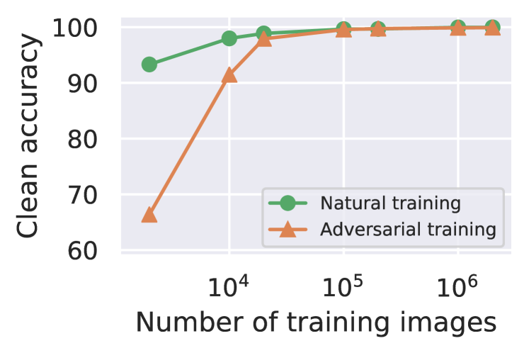
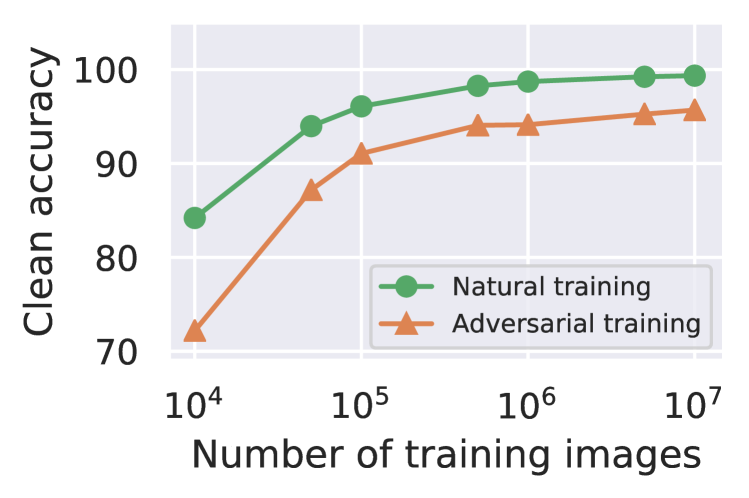
Accuracy vs robustness trade-off. We compare the clean accuracy achieved with both natural and adversarial training in Figure 9. Indeed with a very small number of samples, clean accuracy in adversarial training is traded to achieve robustness. This is evident from the gap between the clean accuracy of natural and adversarial training. However, with the increasing number of training samples, this gap keeps decreasing for both CIFAR-2 and CIFAR-10 datasets. Most interestingly, this trade-off almost vanishes when we use a sufficiently high number of training samples for the CIFAR-2 classification.
On sample complexity of adversarial training. We report both clean and robust accuracy with adversarial training in Figure 9. We find that both clean and robust accuracy continues to improve with the number of training samples. We also observe non-trivial generalization to test images from the CIFAR-10 dataset, which also improves with the number of training samples. Both of these results suggest that even with a small capacity network, such as ResNet-18, adversarial robustness can continue to benefit from an increase in the number of training samples.
D.2 Exploring effect of image quality of synthetic samples
We explore different classifiers to label the unlabeled synthetic data generated from the DDPM model. In particular, we use BiT (Kolesnikov et al., 2020), SplitNet (Zhao et al., 2020), and LaNet (Wang et al., 2019) where they achieve %, %, and % clean accuracy, respectively, on the CIFAR-10 dataset. We notice that labels generated from different classifiers achieve slightly different downstream performance when used with adversarial training in the proposed approach. We find that only up to % of synthetic images are labeled differently by these networks, which causes these differences. On manual inspection, we find that some of these images are of poor quality, i.e., images that aren’t photorealistic or wrongly labeled and remain hard to classify, even for a human labeler. Since filtering millions of images with a human in the loop is extremely costly, we use two deep neural networks, namely LaNet (Wang et al., 2019) and SplitNet (Zhao et al., 2020), to solve this task. We avoid using labels from BiT as it requires transfer learning from ImageNet (Deng et al., 2009) dataset, whereas our goal is to avoid any dependency on extra real-world data. We discard an image when the predicted class of both networks doesn’t match and it is classified with less than 90% confidence by both networks. While the former step flags images which are potentially hard to classify, the latter step ensures that we do not discard images where at least one network is highly confident in its prediction. We also try the % and % confidence threshold but find that % gives the best downstream results. In particular, using the filtering step improves robust accuracy by another %.
