Bayesian statistical framework for identifying
strongly lensed gravitational-wave signals
Abstract
It is expected that gravitational waves, similar to electromagnetic waves, can be gravitationally lensed by intervening matters, producing multiple instances of the same signal arriving at different times from different apparent luminosity distances with different phase shifts compared to the unlensed signal due to lensing. If unaccounted for, these lensed signals will masquerade as separate systems with higher mass and lower redshift. Here we present a Bayesian statistical framework for identifying strongly lensed gravitational-wave signals that incorporates astrophysical information and accounts for selection effects. We also propose a two-step hierarchical analysis for more efficient computations of the probabilities and inferences of source parameters free from shifts introduced by lensing. We show with examples on how changing the astrophysical models could shift one’s interpretation on the origin of the observed gravitational waves, and possibly lead to indisputable evidence of strong lensing of the observed waves. In addition, we demonstrate the improvement in the sky localization of the source of the lensed signals, and in some cases the identification of the Morse indices of the lensed signals. If confirmed, lensed gravitational waves will allow us to probe the Universe at higher redshift, and to constrain the polarization contents of the waves with fewer detectors.
I Introduction
As gravitational waves propagate through the Universe to the Earth, they can be deflected, or lensed, by intervening matters such as galaxies or galaxy clusters acting as gravitational lenses, just like electromagnetic waves. For visible light coming from a distant background source, in the case of strong lensing where the deflection is sufficiently large, multiple images of the source will be formed that are close to each other, typically separated by only several arcseconds and distorted compared to the unlensed image [1]. For transients, the time variation of the images are correlated and delayed, where the time delays range from days to months [1]. For transient gravitational-wave (GW) signals, such as those emitted from coalescences of compact binary systems, multiple images refer to multiple GW triggers registered at different times by GW detectors.111We use the term image and signal interchangeably. For an in-depth review on strong lensing of explosive transients across the electromagnetic-wave (EM) and the GW spectra, see for example Ref. [2].
To investigate the effects of strong lensing on a GW signal, we first briefly describe how the observed GW strain depends on some parameters when the signal is not affected by strong lensing.222Here we use as a placeholder to denote any generic set of parameters, which can consist of different parameters in different contexts. The GW strain observed by a laser-interferometric GW detector is given by
| (1) |
where the detected GW strain is a projection along the arms of the detector where the response of the detector to the two polarization states of the GW is defined by the detector’s beam pattern functions , where is the right ascension, is the declination, and is the polarization angle of the source respectively.333Note that the beam pattern functions are usually calculated in a frame where the detector is situated at the origin, where the angles and are celestial coordinates. Therefore, the beam pattern functions depend implicitly on the time of the event as well. The luminosity distance to the source is a function of the redshift and depends explicitly on the cosmology. The time and phase at coalescence of the signal are denoted by and respectively. The waveform of the two polarization states and can be compactly written as
| (2) |
where depends on some intrinsic parameters and the source redshift only, and is the spin-weighted spherical harmonic that depends on the polar angle and the azimuthal angle in the source frame.444For nonprecessing binary systems, the angle is also known as the inclination angle, the angle between the line of sight and the orbital angular momentum vector, which is by convention chosen to be along the -axis of the source frame. For generic precessing binary systems, the inclination angle changes over time as the orbital angular momentum vector precesses around the total angular momentum vector.555Note that the phase at coalescence does not enter Eq. (2) explicitly but through the time-varying azimuthal angle , with as the reference phase.
For the case of GWs from quasicircular binary black hole (BBH) mergers, the set of intrinsic parameters where is the chirp mass of the binary, is its mass ratio, both in terms of the binary component masses . The vectors , are the dimensionless spin vectors for the binary components. Note that this is just one particular parametrization, and other ways of specifying the intrinsic parameters are also possible; for example, using the total mass of the binary instead of the chirp mass . To account for the effect of an expanding universe, one can do so by simply replacing the (source-frame) masses with the (detector-frame) redshifted masses . Similarly, we define the redshifted chirp mass as , while the mass ratio remains unchanged. It should be noted that Eqs. (1) and (2) hold true regardless of the type of the binary system under consideration, and in general the set of intrinsic parameters will differ for each type of binary systems.
Working in the geometric optics limit where the wavelength is much shorter than the lens length scale, for a majority of the time, strongly lensed GW signals from a binary system will have the same morphology with different amplitudes (corresponding to different magnifications) and arrive at different times. A given image has an absolute magnification which can be defined in terms of the true luminosity distance to the source and the apparent luminosity distance as
| (3) |
where the bracketed superscript indexes the images. The lensed images arrive at the (center of the) Earth at different times because of the geometrical time delay, as they follow different null trajectories, and the time delay due the gravitational potential. We define the relative time delay between two images as , where is the GW arrival (trigger) time for each image. Here we assume that the time delay is large enough so that the lensed images will not overlap with each other and that we can identify them as separate triggers. We refer to the image that arrives first as the first image, and vice versa, such that . We can also define the relative magnification , which is simply the ratio of the two absolute magnifications as
| (4) |
The strong lensing of GW can also induce nontrivial effects on the GW waveform other than a change in the amplitude of the signal and a simple shift in time. In general, the lensed waveform is related to the unlensed waveform by a frequency-dependent amplification factor as [1, 3]
| (5) |
for . The negative frequency components can be obtained via the reality condition . In the geometric optics limit, the amplification factor is given by [1, 3]
| (6) |
for and is known as the Morse index of the th image [1].666Unlike Ref. [4], we did not include the factor explicitly in Eq. (6). This is because by imposing the reality condition on to obtain the negative frequency components, adding an additional will have no effect to the final expression for the waveform. The factor causes the apparent luminosity distance to differ from the luminosity distance of the source, and the phase factor causes the aforementioned time delay. The frequency-independent phase shift from is degenerate with a shift in the phase at coalescence when we consider GW signals from nonprecessing binaries with contributions only from the quadrupole modes [4, 5]. When the geometric optics approximation breaks down and the full wave optics treatment is needed, the expression for the amplification factor can be much more complicated than Eq. (6), and encodes more information about the gravitational lens [1, 3].
Previous works have shown that the detection rate for lensed GWs could be, optimistically, [6] for Advanced LIGO [7] and Advanced Virgo [8] operating at their design sensitivities, while others predicted more pessimistic rates, ranging from [9] to [10] depending on the source population model assumed. The detection rate for lensed GWs can also be constrained from the detection, and more surprisingly the nondetection, of stochastic gravitational-wave background from individually unresolvable binaries [11, 12]. Searches on the first observing run (O1) and the second observing run (O2) data for strongly lensed GW signals were performed [13, 14, 15], and it was concluded that there is no significant evidence that any of the eleven detected GW events during O1 and O2 are lensed, while Ref. [16] suggests that GW170809 and GW170814 could be lensed images of each other due to the similarity of the waveforms for these two events.
It is also possible that strongly lensed GW signals from distant sources are absolutely de-magnified (), or relatively demagnified () such that when found by matched-filtering search pipelines (such as GstLAL [17, 18] and PyCBC [19]) they appeared to be subthreshold triggers, not statistically significant enough to claim detections. If a lensed image is loud enough to be detected individually, then targeted matched-filtering based searches can be performed for each detected GW event and search deeper for its potentially subthreshold lensed image counterparts [20, 21, 14].
An overarching approach in searches for lensed GW signals is the use of Bayesian statistics [22, 13, 21, 15, 14], where a statistic, either called a “Bayes factor” in the usual context of Bayesian hypothesis testing or a ranking score, is calculated. In this paper, we present a Bayesian statistical framework for identifying strongly lensed GW signals that utilizes hierarchical Bayesian modeling. By modeling the data generation processes when the observed GW signals are lensed and not lensed respectively, we develop a framework that allows us to compute a Bayes factor, and hence a posterior odds, that incorporates astrophysical information directly and accounts for selection effects. We argue that in order to interpret the Bayes factor properly as a ratio of normalized probability densities of the observed data, selection effects cannot be ignored and must be accounted for in order to normalize the probability densities. The ability to directly incorporate astrophysical information, both on the GW sources as well as the gravitational lenses, serves to better bridge the astrophysical modeling community and the GW data analysis community. In addition, we argue that whether a GW signal is interpreted as lensed or not depends also on the astrophysical models assumed, making the prior astrophysical information an indispensable ingredient of the analysis.
The paper is structured as follows: Section II presents the hierarchical Bayesian framework for identifying strongly lensed GW signals in a general setting, and the technique to marginalize over the source redshift separately and infer the true source parameters. In Sec. III and Sec. IV we apply and showcase the statistical framework to analyze strongly lensed GW signals from BBH mergers when we analyze two GW signals jointly and analyze one signal at a time respectively. Throughout the paper, we assume a flat CDM cosmology with and from the Planck 2015 results [23].
II Statistical framework
In order to differentiate strongly lensed GW signals from GW signals that are not lensed, we adopt a Bayesian statistical framework where we introduce two models/hypotheses777We will use the word model and hypothesis interchangeably throughout the paper. that we want to compare; namely, the lensed hypothesis and the not-lensed hypothesis .888The not-lensed hypothesis is often referred as the unlensed hypothesis, denoted by , in literature. Here we reserve the meaning of unlensed for effects due to lensing being reverted. The framework applies for , where is the number of GW events under consideration, unlike much of previous work [22, 13, 21, 15, 14]. In the following we will elaborate on what we mean by the two hypotheses, and model the data generation processes under the two different hypotheses using hierarchical Bayesian modeling.
II.1 The not-lensed hypothesis
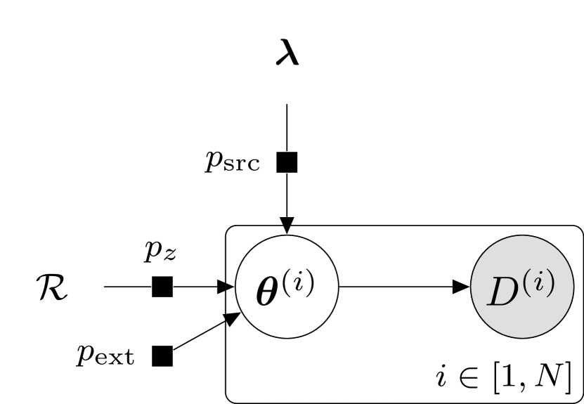
Suppose we have GW events under consideration, i.e., we have a set of time series data , where the bracketed superscript indexes the events. The not-lensed hypothesis means that the observed events are independent realizations of a population distribution of GW source , parametrized by some parameters that control only the shape of the distribution and the total number of sources in that population.999Note that the source population distribution is normalized such that . Note that we have assumed all of them are of astrophysical origins. Simply put, the events are just different systems, with the event-level parameters (such as component masses and spins) describing the th event being randomly drawn from a source population distribution , where might be for example the maximum mass of a black hole in that population. These signals will have different source redshifts drawn from the distribution , where is the merger rate density that can be a function of the source redshift , and with different extrinsic parameters such as the sky location drawn from the distribution . A concise way of expressing this is that where is the population-informed prior distribution under the not-lensed hypothesis. The event-level parameters then in turn “generate” the data that we observed for the th event. Figure 1 shows a graphical representation of this data generation process. Although we are not making any inference on the population-level parameters of GW sources and instead we fix them in our analysis (i.e. choosing and a priori), we see that the problem of identifying strongly lensed signals can be naturally framed as a population analysis. Moreover, we can reuse many of the results from rates and population analyses (for example see Refs. [24, 25]).
II.2 The lensed hypothesis
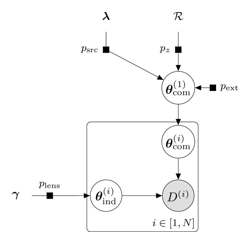
For the lensed hypothesis, suppose we also have the same events under consideration. However, the lensed hypothesis means that these events are actually strongly-lensed images of the same source. Instead of drawing independent realizations from the population distribution , now we only have one realization of this source population distribution as the images correspond to the same GW source. In addition to the source population distribution, we will need to introduce the lens population distribution , parametrized by some parameters , that describes for example the joint probability distribution of the absolute magnification of lensed images. Furthermore, we partition the event-level parameters into two disjoint sets: common parameters and independent parameters . For the common parameters we expect them to be the same across the signals, for example the masses and spins of the source binary system, as the events correspond to the same source. In addition to the source parameters, we also expect the redshift of each image to be the same as the source redshift as strong lensing is achromatic, leaving the redshift unchanged. For extrinsic parameters, we can also assume them to be the same except for the (apparent) luminosity distance and the time of arrival. While it is true that strong lensing will deflect a GW signal from its original null trajectory, the typical deflection angle for gravitational lensing due to a galaxy or a galaxy cluster is only of the order of arcseconds and arcminutes respectively [1, 26], which is much smaller than the typical uncertainty in the source localization of a GW signal. Therefore, it is valid to assume that the images share the same sky location. We also expect the difference in the polarization angle to be negligible [27]. In summary, the common parameters are one random draw of the distribution , where is the population-informed prior for the common parameters under the lensed hypothesis.
As for the independent parameters , we expect them to be different for each event. For example, the absolute magnification and the arrival time of each image would be different. Note that the dimension of the event-level parameters under the lensed hypothesis can be different than that under the not-lensed hypothesis. For example, different lensed images can be classified into three types where each type of an image will have a different phasing effect to the lensed waveform [for example see Eq. (6)]. The number of lensed images produced by a gravitational lens can also inform us on the type of lens that produces the images. Here we do not use this information since it is possible (and often the case) that we are only analyzing a subset of lensed images coming from a particular source and lens, either deliberately or simply because we did not observe all of the lensed images. In short, each image will take different values for the independent parameters where each of them is a random realization of the distribution .
Figure 2 shows a graphical representation of this data generation process. Again one should note that we are not making any inference on the population-level parameters of the GW sources and lenses. Instead we consider them as given in our analysis. Next, we will use our knowledge of the data generation processes under the two hypotheses to construct a statistic that would allow us to evaluate whether some GW signals are lensed or not.
II.3 Model comparison
The standard approach to perform a Bayesian model comparison is to compute the posterior odds , which is defined as101010We will abuse the notation and use to denote both probability and probability density when the context is clear.
| (7) |
Note that for both models we fix the population-level parameters and the merger rate density, and that they are identical for both the lensed and the not-lensed hypothesis. Therefore we will not write them out explicitly when there is no ambiguity. Using Bayes’ theorem, we can easily re-write the posterior odds into a product of two terms, namely the Bayes factor and the prior odds as
| (8) |
We first focus on getting an expression for evaluating the Bayes factor from the set of observed data. And later we will discuss the evaluation of the prior odds .
II.4 The Bayes factor
The Bayes factor , defined as
| (9) |
is a ratio of the normalized probability densities of observing the data set assuming the two hypotheses under consideration. In Appendix A we give the full derivation for the expressions evaluating the normalized probability densities of observing the data set under each of the hypotheses. Here we will outline the derivation. The core idea is to use the graphs that describe the data generation processes for the two hypotheses in Figs. 1 and 2 to write down the desired expressions for the probability densities, and that the likelihood functions (which are the probability densities viewed as functions of the event-level parameters) can be factorized under both the hypotheses.
For the not-lensed hypothesis, since the signals are independent, we have
| (10) |
Combining this with the data generation process described in Fig. 1 we have
| (11) |
where the expression on the right-hand side is also known as the (unnormalized) marginal likelihood under the not-lensed hypothesis. Note that we need to make sure that the probability density is normalized over all observable111111Here the term observable data means that the signals in the data would pass some detection criteria that one imposes, for example the signals would need to have a signal-to-noise ratio above some threshold, such that they would be identified as GW events. data, accounting for selection effects [28]. This can be done by evaluating the proper normalization constant , where
| (12) |
Therefore the expression for the normalized is given by
| (13) |
As for the lensed hypothesis, unfortunately the probability density cannot be factorized like Eq. (10). However, the likelihood functions can still be factorized if we assume that the noise realizations for the events are independent and that a signal is deterministic given a set of parameters that describe the waveform. Marginalizing the joint likelihood function with parameters according to Fig. 2, we have
| (14) | ||||
where the expression on the right-hand side is known as the (unnormalized) marginal likelihood under the lensed hypothesis. Again, we will need to compute the normalized probability density in order to compute a meaningful Bayes factor, and take selection effects into account. The proper normalization constant in this case, is given by
| (15) | ||||
Therefore, the expression for the normalized is given by
| (16) | ||||
Finally, we have the expression that we can use to evaluate the Bayes factor for the lensed hypothesis versus the not-lensed hypothesis, namely
| (17) |
One can interpret the second factor in Eq. (17), which is the ratio of unnormalized marginal likelihoods under the two hypotheses, as a measurement of how well the data set of signals can be jointly fit by a set of common parameters versus sets of independent parameters, which we call it the coherence ratio to differentiate it with the Bayes factor. While a negative log-coherence ratio means that the lensed hypothesis, that is setting some of the parameters to be the same across events, fails to fit the signals jointly, a positive log coherence ratio however does not mean that the signals are lensed. This is the Occam’s razor at play. Assuming that the lensed hypothesis and the not-lensed hypothesis fit the data set equally well, the lensed hypothesis will be favored by the Bayesian model selection framework because it has fewer free parameters, and hence a smaller prior volume. For GW signals from high-mass BBH mergers, this issue will be more apparent as they produce shorter signals detectable in the interferometers, and we usually make less precise measurements of the masses for these high-mass systems [29]. This is partially alleviated by incorporating the population information that they are rarer compared to lighter systems. It also brings out an important point that the Bayes factor, or generally any probabilistic statement, that some GW signals are strongly lensed depends on the source population one is considering.
We can think of the factor in Eq. (17) as a population-averaged scale of the coherence ratio accounting for selection effects, which affect the two hypotheses differently. If the coherence ratio is greater than the population typical value for , then the Bayes factor will indicate that the lensed hypothesis is favored by the observed data. In fact, the normalization constant under the not-lensed hypothesis can be interpreted as the detectable fraction of sources [28]. Similarly, we can interpret the normalization constant under the lensed hypothesis as the fraction of sources that would produce detectable lensed signals. We expect that the order of magnitude for would be similar to that for . Therefore, essentially selection effects penalize the lensed hypothesis by a factor of roughly , counteracting the Occam’s razor.
II.5 The prior odds
The Bayes factor we derived above in Eq. (17) only compares the coherence of the data set with each hypothesis, but not the probability in which each hypothesis would occur. We know empirically, that strong lensing causing at least images occurs less frequently than observing independent GW events with each coming from a different source. We can incorporate our knowledge about the rate in the form of prior odds , which is defined as
| (18) |
We can then compute the posterior odds using Eq. (8) from the Bayes factor in Eq. (17) and the prior odds in Eq. (18).
One can assign the prior odds simply as the ratio of the rate of observing lensed images from a single source over the rate of observing GW signals coming from independent sources. Obtaining this will require detailed modeling of GW sources and lenses. In particular these numbers should be computed under the the chosen source and lens population models for an analysis. However, one can argue that for most of the population models commonly used by the astrophysics community, the prior odds is very small with the current sensitivities of GW detectors, about [6, 9, 10, 11, 12].
II.6 Marginalization over redshift
With the expression for under the lensed hypothesis in Eq. (16), one can estimate the integral using a stochastic sampling algorithm such as nested sampling [30] by sampling over with a prior and a joint likelihood . However, a direct sampling will be inefficient because of the degeneracy between the absolute magnification and the luminosity distance, and hence the redshift of the source. Under the not-lensed hypothesis, we can infer the source redshift since we can infer the luminosity distance of the source , and by assuming a particular cosmology we can compute the redshift from the luminosity distance. Under the lensed hypothesis, each image will be, in general, magnified by a different factor. In fact, we can only measure the apparent luminosity distance for each image as in Eq. (3). Therefore, we will not be able to infer the absolute magnification for each image and the source redshift at the same time. For example, a signal with a said redshift of and an absolute magnification of would have the same apparent luminosity distance of Gpc as a signal with a redshift of and an absolute magnification of .
In order to explore the degenerate parameter space more efficiently, we can marginalize over the source redshift separately. In fact, the source redshift stands out from the rest of the parameters. This is because with a given redshift, one can figure out the prior distribution of the apparent luminosity distance given the prior distribution of the absolute magnification by
| (19) | ||||
and similarly for the prior distribution of the redshifted/detector-frame masses given the distribution of source-frame masses and the redshift as
| (20) | ||||
Therefore, we can rewrite Eq. (16) as a 1D integral over the redshift as
| (21) |
where is given by
| (22) | ||||
The marginalized likelihood , which is a function of only, can be obtained via the conventional Monte Carlo methods (such as Markov Chain Monte Carlo method and nested sampling) by sampling over redshifted/detector-frame parameters without the redshift. This will alleviate the degeneracy problem, as well as open up the possibility of computing Eq. (16) by reusing computations done with the not-lensed hypothesis assumed, without re-exploring the joint parameter space. It also lends itself to the interpretation of treating the redshift as a hyperparameter of a subpopulation of signals sharing the same intrinsic parameters (and some of the extrinsic parameters).
Given a merger rate density , which is the number density of mergers per comoving volume per unit time in the source frame, one can compute the probability density of the source redshift as
| (23) |
Using the product rule, we can write down the prior distribution for the redshift under the lensed hypothesis as
| (24) | ||||
where is the normalization constant, and is the optical depth of strong lensing at redshift . Similarly, under the not-lensed hypothesis, the prior distribution for the redshift is given by
| (25) | ||||
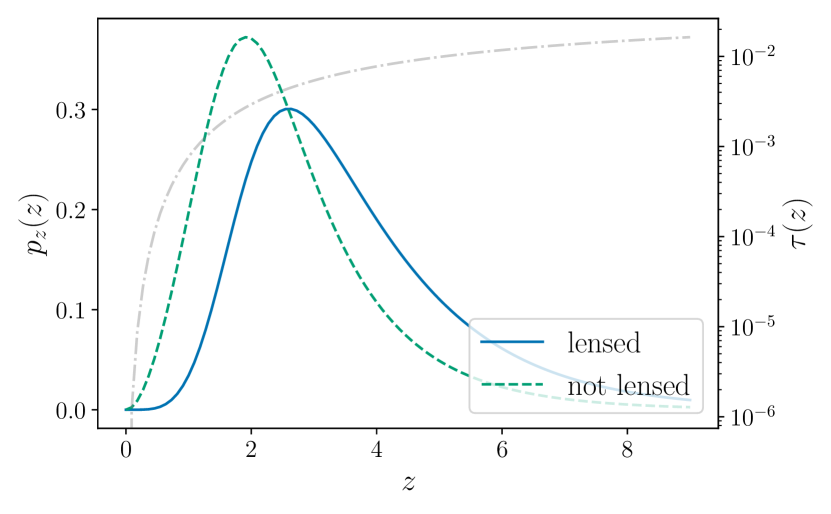
where the normalization constant is defined accordingly. Figure 3 shows the prior distribution of redshift under the lensed (solid blue line) and not-lensed hypothesis (dashed green line), using the optical depth model in Ref. [13] and a merger rate density tracking the star formation rate in [31, 9]. The peak of the prior distribution under the lensed hypothesis shifts to a higher value of compared to that under the not-lensed hypothesis, which peaks at roughly because of the optical depth (gray dash-dotted line) being higher at higher redshifts.
As a by-product of evaluating Eq. (21), we also get a set of posterior samples of , which are distributed according to
| (26) |
In the next subsection, we describe how to reconstruct the true (but degenerate) source parameters using Gibbs sampling.
II.7 Inferring source parameters using Gibbs sampling
Ultimately we want a set of joint posterior samples describing the source of the observed lensed signals. As a by-product of the marginalization over the redshift calculation using nested sampling, we obtain a set of posterior samples of the redshift marginalized over the parameters . Using Gibbs sampling, we can obtain the desired joint posterior samples from samples drawn from the conditional probability distributions from the marginalization step and from the inference step. This is because
| (27) |
Algorithm 1 outlines the (collapsed and blocked) Gibbs sampling algorithm [32] that allows us to reconstruct the joint posterior samples. This variant of Gibbs sampling can be easily parallelized since each iteration is independent. For each set of joint samples, since are redshifted parameters (such as the redshifted component masses) and is the source redshift, one can compute the true source parameters such as the source masses easily. In Sec. III, we demonstrate the framework and tools we developed with simulated lensed GW signals from BBH mergers.
III Strong lensing of gravitational waves from a binary black hole merger: observing a pair of lensed signals
Now that we have developed the statistical framework in a general setting, here we want to apply the framework to analyze two particular cases and discuss the technical subtleties involved, namely for the case of strong lensing of a GW signal from a BBH merger with a pair of lensed images (i.e. ) observed, and with only one image (i.e., ) observed. In this section, we focus on the former case first.
III.1 Under the not-lensed hypothesis
Suppose we write the event-level parameters for each of the BBH mergers under the not-lensed hypothesis as
| (28) |
and these are the parameters that are being sampled over during the inference step. As derived in Eq. (13) with , under the not-lensed hypothesis we have
| (29) | ||||
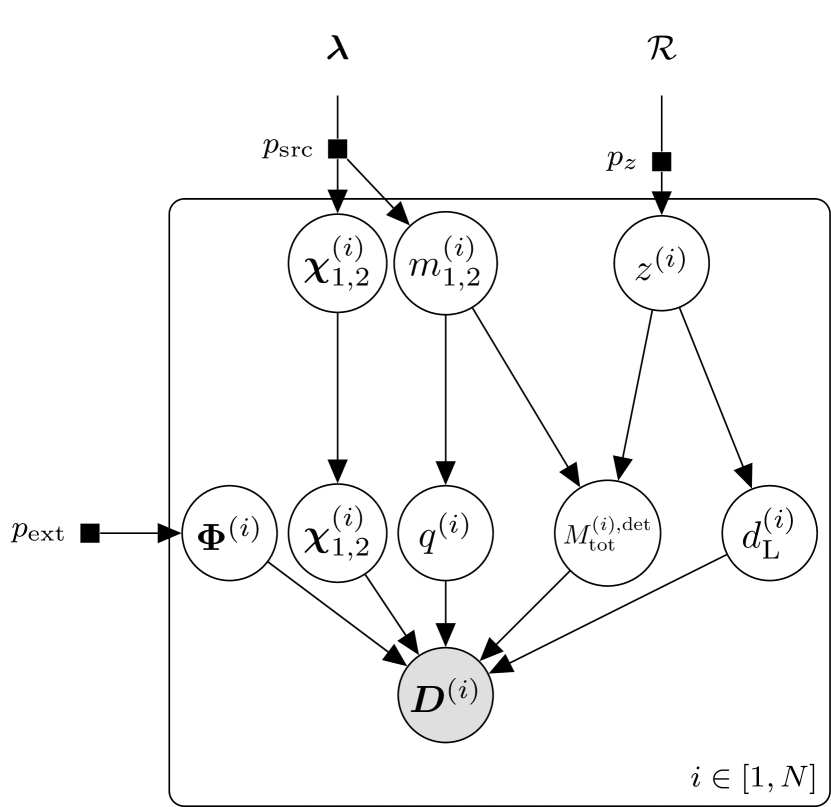
Figure 4 shows a graphical representation of the data generation process under the not-lensed hypothesis for signals from BBH mergers using the parametrization in Eq. (28). Here we use to denote the set of extrinsic parameters that are distributed according to the distribution . As for the time of arrival , we treat it separately and hence it is not shown in Fig. 4. From matched-filtering pipelines that scan through all the data looking for GW triggers, we know roughly the time of arrival for each trigger. Let us write and , where and are the point estimates of the arrival times given by a pipeline for the two triggers respectively. Instead of sampling over and , we sample over and with a small prior range (typically s) and taken to be known. Mathematically, this means
| (30) | ||||
Suppose we order the two events by their times of arrival, i.e. , and define the time delay . After this transformation, there is an extra factor in the prior that accounts for the probability of having two random events separated by a time delay of under the not-lensed hypothesis. If we model the arrival of events by a Poisson process, the prior probability density that any random pair of events having a time delay of , given that there are events during the time interval of , is given by
| (31) |
where we give a detailed derivation in Appendix C. This can be considered as the part of the time-delay Bayes factor in Ref. [22] from the not-lensed hypothesis.
Therefore, the full expression for now reads
| (32) | ||||
where under the not-lensed hypothesis there is a one-to-one mapping between and , and hence one will only need to convert Eq. (25) by multiplying the proper Jacobian without the need of a separate marginalization of the source redshift.
III.2 Under the lensed hypothesis
Under the lensed hypothesis, we write the event-level parameters differently, namely we let the common parameters . As for the independent parameters, we write , where we perform the same transformation to the time of arrival as in the case under the not-lensed hypothesis, and denotes the type of an image which can be either {I, II, III}.
Each strongly lensed image can be classified into three types (I, II or III), where each image type corresponds to a Morse index of respectively, inducing a different phase shift as shown in Eq. (6) to the image because of the interaction of the lensed image with the caustic. One would expect the image that arrives at the Earth first to be of type I since type-I images correspond to local minima of the Fermat time-of-arrival potential. However, the signal that we called the first image in an analysis might not actually be the first image that had arrived the Earth since, for example, the GW detectors might be offline. Various arguments on the type of images one would see can be made if we know the geometry of the gravitational lens but this is not known prior to the analysis. Therefore, to be lens-model-agnostic we assume that the type of the lensed images in a pair to each follow a discrete uniform distribution and are uncorrelated, namely
| (33) |
where
| (34) |
That being said, both the assumptions that the image types are uncorrelated and each follows a uniform distribution are not true. If one adopts a particular lens model and ordering of the images, the appropriate joint distribution that encapsulates the correlation should be used instead.
Figure 5 shows a graphical representation of the data generation process under the lensed hypothesis for BBH signals. Similar to Fig. 4, we use to denote the set of extrinsic parameters that are distributed according to the distribution , and that we treat the time of arrival separately. Unlike the not-lensed case, here we assume that are the same across the signals (hence we dropped the superscript in the graph). Also, even though we sample the apparent luminosity distance for each image, there is no one-to-one mapping between it and the true source redshift since the apparent luminosity distance is also related to the absolute magnification of a lensed image. As discussed in Sec. II.6, we perform the marginalization over the source redshift separately.
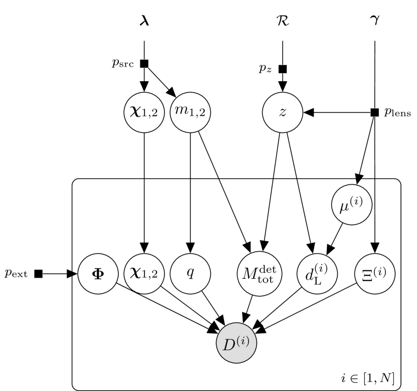
For the time of arrival , we can perform the same transformation as in the case for the not-lensed hypothesis (similar to Eq. (30)), and sample that has a much smaller range instead. However, instead of having an analytical expression for the time delay , there is no analytically tractable expression for the time delay under the lensed hypothesis. That being said, we can obtain it readily from numerical simulations (for example, Ref. [22]). As a result, there is an extra factor of in the prior that accounts for the probability of having two lensed images separated by a time delay of .
Therefore, the full expression for now reads
| (35) | ||||
where the expression enclosed by the square brackets would be identified as as discussed in Sec II.6.
III.3 Demonstration
Here we demonstrate the framework with two examples. In the first example, we injected two GW signals with a redshifted total mass into simulated data streams. With this example, we show explicitly how the source population model would change the Bayes factor. In the second example, we injected instead two GW signals with a redshifted total mass , which corresponds to typical stellar-mass BBH systems for the LIGO-Virgo detectors. In both examples, we use the waveform approximant IMRPhenomXPHM [33], which models both the leading-quadrupole () radiation, as well as some of the nonquadrupole () multipoles. By incorporating the higher-order modes, we show that the image type of each lensed signal can also be inferred. All the results presented here were computed using the software package hanabi121212https://github.com/ricokaloklo/hanabi, which is built upon the package bilby [34] and parallel_bilby [35]. Also, we used the nested sampling algorithm implemented in the package dynesty [36] with the number of live points and the number of autocorrelation times when running the nested sampling algorithm, where the settings are sufficient to give convergent results [37]. More specifically, the results presented in this paper used the aforementioned packages of version bilby==1.0.2 [38], parallel_bilby==0.1.5 [39], dynesty=1.0.1 [40], and hanabi==0.3.1 [41].
III.3.1 Example 1: Two lensed signals from apparent intermediate-mass binary black hole mergers
In this example, we have two lensed GW signals injected into two simulated data streams with Gaussian noise recolored to match the Advanced LIGO (aLIGO) design noise curve [42]. Table 1 summarizes some of the waveform parameters for the two signals. The two injected signals, when analyzed on their own, seem to originate from two separate mergers of an intermediate-mass binary black hole system.
| Parameter | Value |
|---|---|
| Redshifted total mass | |
| Mass ratio | |
| Redshifted primary mass | |
| Redshifted secondary mass | |
| Dimensionless spin magnitude of the primary | 0.3 |
| Dimensionless spin magnitude of the secondary | 0.2 |
| Tilt angle between the spin vector of the primary | rad |
| and the orbital angular momentum vector | |
| Tilt angle between the spin vector of the secondary | rad |
| and the orbital angular momentum vector | |
| Azimuthal angle between the two spin vectors | rad |
| Azimuthal angle of the cone of precession of the orbital | rad |
| angular momentum about the total angular momentum | |
| Inclination angle between the total angular momentum | rad |
| and the line of sight | |
| Right ascension | rad |
| Declination | rad |
| Polarization angle | rad |
| Phase at coalescence | rad |
| Apparent luminosity distance for the | 3.11 Gpc |
| first signal | |
| Apparent luminosity distance for the | 3.15 Gpc |
| second signal | |
| Image type of the first signal | I |
| Image type of the second signal | II |
To demonstrate how using different source population models would change one’s interpretation of the two signals, as well as the numerical value of the Bayes factor using our framework, we first use a log-uniform distribution as the population model for the component masses, namely
| (36) |
For the component spins, we use a distribution that is uniform in the component spin magnitude, and isotropic in the spin orientation.
As for the merger rate density, here we use, for the sake of demonstration, an analytical fit from Ref. [9] that tracks the population synthesis results from Ref. [31] for population-I and population-II stars, namely
| (37) |
For the absolute magnification, again for the purpose of demonstration, we use a simple power law distribution that is independent of the time delay, namely
| (38) |
with
| (39) |
where it captures the general scaling in the high-magnification regime, as well as the requirement that the absolute magnification has to exceed some threshold in order for multiple lensed images to be formed. However, it does not capture the correlation between the magnifications of the lensed images, and the correlation between the magnification and the time delay. For example, the relative magnification tends to unity if the lensed images are highly magnified [1]. In fact, one can derive a poor-man’s prior distribution for the relative magnification, if we assume that the absolute magnification for each of the two images follows Eq. (38), with the form
| (40) |
where we give a detailed derivation in Appendix D. The poor-man’s prior distribution for the relative magnification models the correct power law scaling of when , but predicts the wrong power law scaling when .
In addition, we use a simple analytical model for the optical depth [43, 13], which is the probability of strong lensing at a given redshift, with the form
| (41) |
where is the comoving distance at , and is the Hubble distance. The empirical constant is taken to be 0.0017 here [13]. A more realistic and detailed model for the merger rate density, the magnification distribution, as well as the optical depth, that impart more astrophysical information to an analysis would certainly help differentiating lensed signals.
With this set of population models, we obtained a log-coherence ratio of , and a log-Bayes factor of without accounting for the time delay.131313This means that we set such that the coherence ratios and the Bayes factors reported will not be boosted by setting the time-delay of the injected signals to be very consistent with the lensed hypothesis, though incorporating the time delay information would be important in actual analyses. We see that with this set of population models and the detector sensitivity, the selection effects down-weight the pair by a factor of . Figure 6 shows both the 1D and 2D marginalized posterior distributions for obtained using the algorithm described in Sec. II.7. The orange solid lines show the correct values for each of the parameters if the redshift is set to . The plot shows that our two-step hierarchical procedure described in Sec. II.6 is able to find the correct values describing the signals. From the plot we can also see the various degeneracies between parameters. For example, the degeneracy between the total mass and the redshift , where the blob in the lower left corner of Fig. 6 corresponds to the redshifted total mass that we do measure. Note that we are able to infer the mass ratio and the relative magnification as they are not degenerate with the redshift.
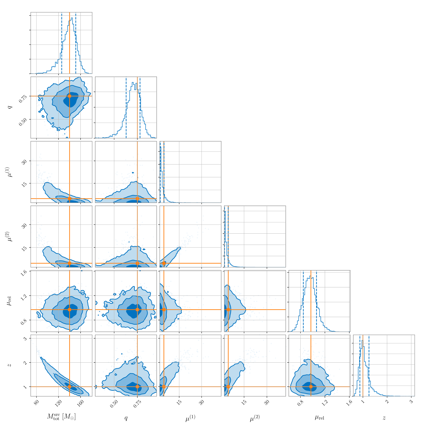
If we instead use a population model that asserts there are no black holes with mass greater than , referred as “Model A” in Ref. [24], namely
| (42) |
with , , , and 141414Note that the numbers we adopted here are slightly different from the reported values in Ref. [24] because we write the model in the parametrization here instead of the parametrization. The probability density is hence off by a Jacobian of , which can be easily accounted for by adjusting the value of ., now both the log-coherence ratio and the log-Bayes factor are infinite, while the log evidence under the lensed hypothesis is finite. This is a “smoking-gun evidence” that the two signals are lensed. This is not surprising because the two signals are impossible under the not-lensed hypothesis with this set of population models. Under the not-lensed hypothesis, we interpret the apparent luminosity distance as the true luminosity distance without any magnification bias, allowing us to infer the redshift directly from the measured luminosity distance. In this case, the redshift that corresponds to the apparent luminosity distance of the first signal is roughly , meaning that both the primary and secondary mass would be above the maximum. This example, though extreme, clearly shows that the Bayes factor, and hence one’s interpretation on the origin, of the signals would be sensitive to the population models that one assumes.
III.3.2 Example 2: Two lensed signals from a stellar-mass binary black hole merger
In the second example, we also have two lensed GW signals injected into two simulated data streams with Gaussian noise. However, this time the two signals have a lower redshifted total mass (). Table 2 summarizes some of the waveform parameters. This example serves to represent typical scenarios for second-generation terrestrial GW detectors such as the two Advanced LIGO detectors [7] and the Advanced Virgo detector [8] observing stellar-mass BBH systems, and demonstrate how would the Bayes factor change with different detector sensitivities. For the population models, we use the same set of models in the last subsection with the “Model A” mass model described in Eq. (42).
| Parameter | Value |
| Redshifted total mass | |
| Mass ratio | |
| Redshifted primary mass | |
| Redshifted secondary mass | |
| Apparent luminosity distance for the | 811 Mpc |
| first signal | |
| Apparent luminosity distance for the | 823 Mpc |
| second signal |
Figure 7 shows the marginalized 1D and 2D posterior distributions for we recover when the two lensed signals were injected into data streams with simulated Gaussian noise recolored to match the aLIGO design sensitivity [42]. From the plot we see similar degenerate structures between parameters as in Fig. 6. To demonstrate the degeneracies more explicitly, we show the correct source parameters for this two signals if we assume the true source redshift is (solid orange lines), as well as that if the true redshift is instead (dotted gray lines). Note that both the mass ratio and the relative magnification take the same value when different source redshifts are assumed. While we are not able to constrain the source parameters individually because of the aforementioned degeneracies, we are capable of providing joint constraints for the source parameters by properly incorporating information from both the detected signals and the astrophysical population models assumed. From Fig. 7, we see that it is less likely for the signals to come from a binary system with a total mass of at a redshift under the lensed hypothesis because of the large absolute magnifications required are less probable under the lens model we assumed in the analysis.
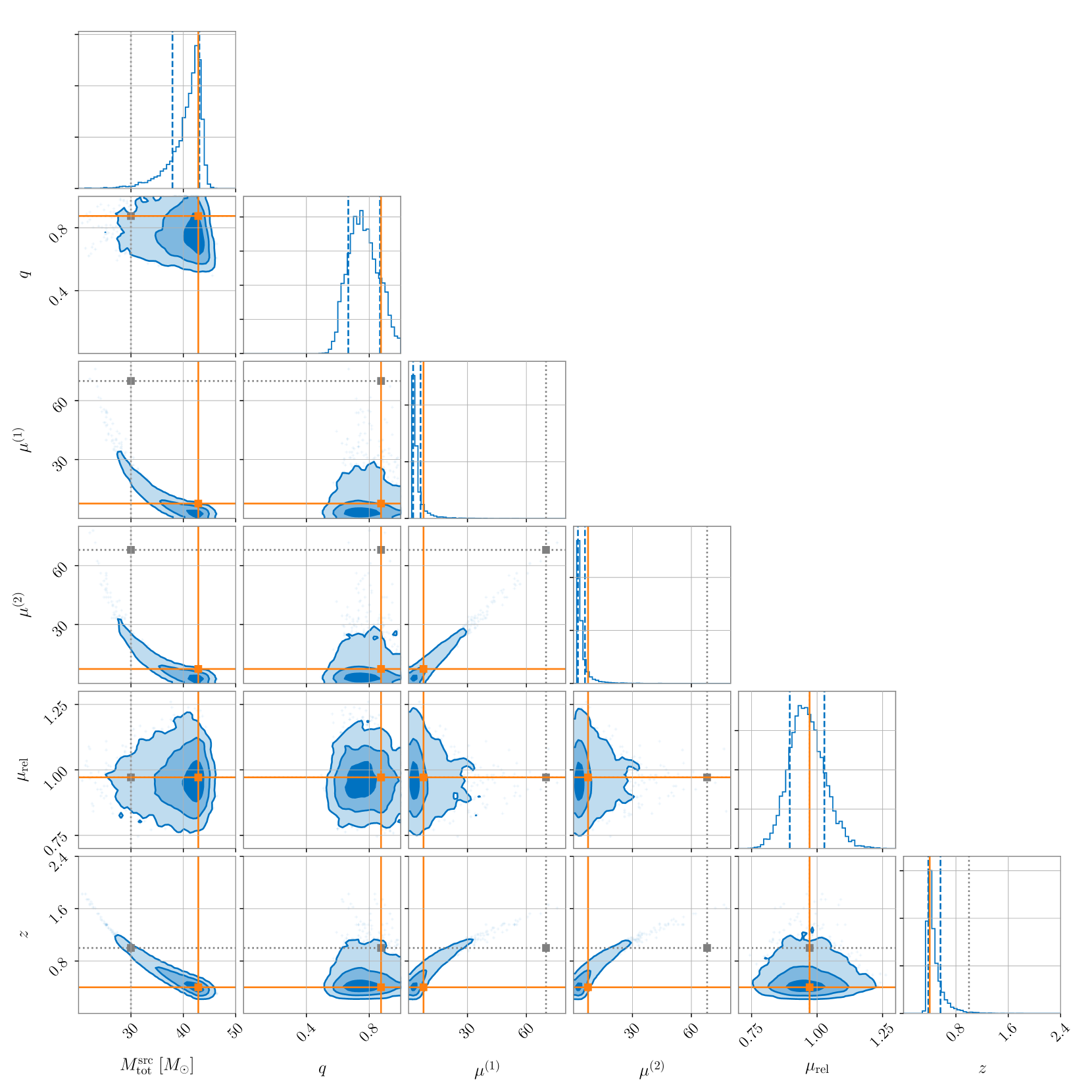
For this example, we obtained a log-coherence ratio of and a log-Bayes factor of when injecting the signals into simulated Gaussian noise recolored to match the aLIGO design sensitivity [42]. Table 3 tabulates the values of , , and for this particular set of population models under different detector sensitivities, computed using pdetclassifier [44]. In Appendix B, we give a detailed description on how one can compute these normalization constants, or selection functions, under the lensed and the not-lensed hypothesis.
| O1+O2 | O3a | aLIGO design | |
| 2.9 | 2.5 | 2.3 |
As expected, the values of and increase as the detector network becomes more sensitive and capable of detecting weaker signals. The difference between the values of and narrows as the network increases in sensitivity, and that the selection effects penalize the lensed hypothesis to a lesser extent, roughly by a factor of . While we did not perform the same injection test with simulated noise recolored to match the sensitivity during O1+O2 and O3a, we can reasonably expect the log-coherence ratio increases with a more sensitive detector network as we can better measure the waveform parameters to a higher precision. Therefore, the log-coherence ratio, as well as the log-Bayes factor would increase with the detector sensitivity given the same set of lensed signals.
III.4 Identifying the image types
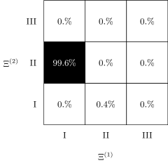
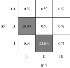
When we consider only the dominant modes and a nonprecessing binary system, the phasing effect due to strong lensing reduces to a shift in the observed phase at coalescence (or any reference orbital phase) [4, 5]. For a GW signal from the merger of a precessing binary system with a significant contribution from higher-order modes, for example when the system is asymmetric in component masses and/or is inclined with respect to our line of sight, we can break the degeneracy between the phasing effect from strong lensing and the orbital phase. This allows us to identify the image type for each of the lensed signals. We demonstrate this by injecting signals with an asymmetric mass ratio viewing at an angle of roughly between the line of sight and the total angular momentum vector into simulated Gaussian noise at aLIGO design sensitivity using two different waveform models, IMRPhenomXP and IMRPhenomXPHM [33]. The former approximant, IMRPhenomXP, includes only the quadrupole () radiation from a precessing binary system, while the latter approximant, IMRPhenomXPHM, includes both the quadrupole radiation and some of the higher multipoles () from the precessing system. In both cases, the first injected lensed GW signal is of type I, while the second injected signal is of type II. Figure 8 shows the joint probability mass function of the image type inferred for the first signal and that for the second signal . We see that when there are measurable contributions from higher modes, we are able to pin-point the type of each lensed image from the phasing effect (left panel of Fig. 8), breaking the degeneracy between the phasing effect from strong lensing and the shift in the orbital phase. This is in line with the findings reported in Ref. [45], where one can tell type-II images apart individually for third-generation detectors.
III.5 Improvement in localizing the source in the sky
Since we expect the lensed GW signals coming from the same source to have approximately identical sky locations, the signals should be better localized when analyzed jointly compared to the case when they are analyzed individually. This is because we gain information about the shared sky location from two data streams instead of just one. We demonstrate this using the inference results from Example 1 in Sec. III.3.1. Figure 9 shows the credible regions of the localization of signals, when analyzed separately (blue and green) and when analyzed jointly (orange). In all cases, the credible regions enclose the true source location (gray crosshair). However, the area of the credible region, a metric for the localization uncertainty, from the joint inference is only , which is roughly two times smaller than that when localizing the first image only () and roughly four times smaller than that when localizing the second, fainter, image only ().
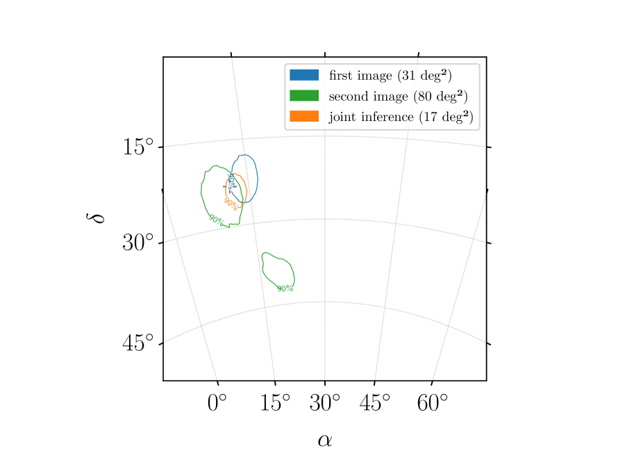
Combining the improved sky localization of the source with the joint constraints of the source parameters (such as the redshift), one will be more informed when trying to locate the gravitational lens and the source electromagnetically (see, for example, Ref. [46, 47]). Indeed, if we were able to identify the massive object responsible for the gravitational lensing and observe lensing of electromagnetic waves as well, that can serve as a cross-validation that the GW signals that were being analyzed are indeed strongly lensed. The lensed source could be by itself electromagnetically bright, for example a binary neutron star system or a neutron-star-black-hole binary (though it is not expected to see lensed signals coming from these kind of sources with current-generation GW detectors as they have lower merger rates relative to BBH systems). If the lensed source is in a host which emits electromagnetic radiation, such as in a galaxy, one could search for possible foreground lenses (as the electromagnetic signature coming from the host should also be lensed by the same lens) within the joint localization region that would produce lensed GW signals with consistent absolute magnifications and time delays.
IV Strong lensing of gravitational waves from a binary black hole merger: observing only one lensed signal
The statistical framework can also be applied when only one GW signal (i.e. ) is being analyzed at a time. In this case, the expression for the Bayes factor reads
| (43) |
where the normalization constant for the case of is defined accordingly. For BBH systems, the data generation process described in Fig. 4 for the not-lensed hypothesis, and that in Fig. 5 for the lensed hypothesis, are also applicable here. Compared with the case of we discussed extensively in Sec. III, the framework is less capable of differentiating a lensed BBH signal in the geometric optics limit from a signal that is not lensed. This is because effectively the framework is leveraging only the inconsistency of the signal with the given population models without the help of Occam’s razor and selection effects. However, this will not be the case if gravitational lensing leaves distinctive signatures in the observed waveforms, for example when the geometric optics approximation breaks down and the full wave optics treatment is needed [1, 3]. The framework can also be easily extended to handle GW lensing from BNS systems (see, for example, Ref. [48]) and NSBH systems.
Here we demonstrate the statistical framework when with an example where a lensed BBH signal with waveform parameters identical to the first image of Example 1 in Sec. III.3.1 (cf. Table 1) injected into simulated Gaussian noise recolored to the aLIGO design noise curve [42]. As we shall see, the framework is less capable of identifying a lensed BBH signal purely from its inconsistency with the population models, unless the models fail to produce such an observed signal (such as Example 1 in Sec. III.3.1 with a source population model asserting that no black hole can have a mass greater than ). This is very similar to the lensing analysis for GW190521 presented in Ref. [49], and the BNS lensing analysis in Ref. [48].
In this example, we first use the log-uniform distribution in Eq. (36) as the population model for the component masses, and use the same models for spin, magnification, optical depth, and merger rate density as in Sec. III.3.1. Figure 10 shows the marginalized 1D and 2D posterior distributions of , again using the Gibbs sampling algorithm described in Sec. II.7. The orange solid lines show the correct values for each of the parameters if the redshift is set to . Similar to the case with in Fig. 6, we observe similar degenerate structures such as that between and . However, the uncertainty in the joint constraint here when is greater compared to that in Fig. 6. This can be attributed to the less constraining measurements of the redshifted masses when there is only one data stream to infer from, instead of two data streams as in the case for Fig. 6.
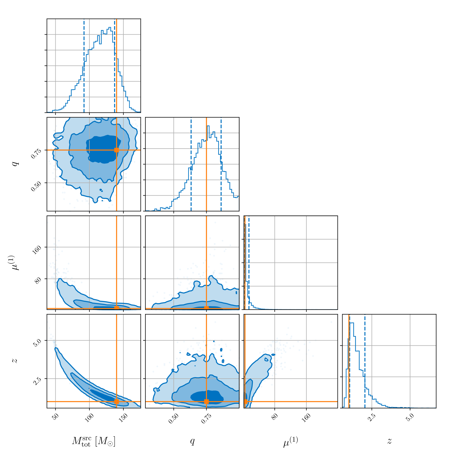
With this set of population models, we obtained a log-coherence ratio of , and a log-Bayes factor of . The Bayes factor here is not statistically significant and within the statistical uncertainty from using nested sampling. Given the rarity of strong lensing, reflected in the prior odds, the strong lensing hypothesis will easily be dismissed with the small posterior odds. While the above example might give a pessimistic impression for identifying strongly lensed BBH signals individually, this does not have to be the case, especially if the signals are of type II, where we might be able to identify them from the distortion to the waveforms due to lensing, for example from the extra Morse phase [45], or other frequency-dependent wave optics effects.
V Conclusions and outlook
In this paper, we present a Bayesian statistical framework for identifying strongly lensed GW signals. By modeling the data generation processes for observed signals assuming that they are lensed images from the same source and that they are simply signals from different sources respectively, we are able to write down an expression for the Bayes factor which quantifies the ratio of the probability densities of observing the signals given the two scenarios and the astrophysical models on the properties of the sources and lenses. Selection effects are accounted for naturally as we normalize the probability densities. Combined with the prior odds, we can properly interpret the resultant posterior odds as the ratio of the probability that the signals are strongly lensed versus not lensed.
In order to compute the marginalization integral for the Bayes factor more efficiently, we present a hierarchical scheme to evaluate the integral over the source redshift separately, breaking down the high-dimensional integral into an integral with a lower dimension and smaller degeneracy among variables that can be computed using Monte Carlo methods such as in Ref. [30], plus a 1D integral over the redshift that can be efficiently evaluated. The true source parameters can be inferred after the hierarchical analysis using a Gibbs sampling algorithm.
We demonstrate the framework with examples when and , respectively. We show explicitly how changing the assumed astrophysical models can alter one’s interpretation on the origin of the observed signals, and sometimes can lead to smoking-gun evidence of strong lensing of GW. For the case of , we also show how one can jointly constrain the total mass and the redshift of the source. Together with the improvement in localizing the source from observing two images, it helps locating the source and the lens electromagnetically [46, 47], and ultimately cross-validating the GW lensing analysis. In some cases where higher multipoles of lensed GW signals are observable, the Morse index, or the type, of the lensed images can be identified.
Currently, one of the key assumptions of the framework is that all triggers are of astrophysical origins. This might not be the case when we perform a targeted search on subthreshold lensed counterparts [20, 21, 14], especially for a high-mass GW signal. This is because transient noise fluctuations in the detectors, or glitches, can easily mimic these short-duration high-mass signals. In this case, unfortunately, the Occam’s razor is working against us as the lensed hypothesis will have a similar goodness-of-fit to the glitches compared to the not lensed hypothesis while having fewer free parameters. The assumption can be relaxed where some of the triggers are of terrestrial origins. However, this would require a detailed study of the morphology of the glitches and we leave this to future work.
While detecting strongly lensed GW signals are exciting in its own right, it can also be used to improve our understanding on various subjects in fundamental physics, astrophysics and cosmology. For example, observing the strongly lensed GW signals from the same source multiple times effectively boosts the number of “virtual GW detectors”, and hence can be used to better constrain the polarization contents of the GW signals and test the general relativity [50]. Strongly lensed GW signals also allow us to probe further to study for example stellar environments at higher redshift through the spin alignment of the lensed binaries [51], and origins of the binaries at high redshift [52, 53]. With the statistical framework presented in this paper, which directly ingests models from the astrophysics community, the GW data analysis community can work closer together with the astrophysical modeling community on finding lensed GWs and extracting more science from them.
Acknowledgements.
The authors would like to thank Tjonnie G. F. Li, Will Farr, Masamune Oguri, Alan Weinstein, Yanbei Chen, Katerina Chatziioannou, Colm Talbot, and Ken K. Y. Ng for the discussion and the help when preparing this paper. R. K. L. L. acknowledges support from the Croucher Foundation. R. K. L. L also acknowledges support from NSF Awards No. PHY-1912594, No. PHY-2207758. I. M. H. is supported by the NSF Graduate Research Fellowship Program under Grant No. DGE-17247915. The computations presented here were conducted on the Caltech High Performance Cluster partially supported by a grant from the Gordon and Betty Moore Foundation. I. M. H. also acknowledges support from NSF Awards No. PHY-1607585, No. PHY-1912649, No. PHY-1806990, and No. PHY-2207728. The authors are also grateful for computational resources provided by the LIGO Laboratory and supported by National Science Foundation Grants PHY-0757058 and PHY-0823459. Figs. 1, 2, 4, and 5 were generated using BayesNet. Figures 6, 7, and 10 were generated using corner.py [54]. This is LIGO Document No. P1900058.Appendix A Full derivation of the probability densities of observing a set of data under various hypotheses
In this section, we give the full derivation for the probability densities of observing a set of data under the lensed hypothesis and the not-lensed hypothesis , accounting for both the astrophysical information on sources and lenses, and well as selection effects. This would in turn allow us to write down the expression for the (proper) Bayes factor and hence the posterior odds for identifying strongly lensed gravitational-wave signals. The derivations below follow Ref. [28] closely.
A.1 Under the not-lensed hypothesis
Now let us find the expression for the probability density under the not-lensed hypothesis . Since each of the observed data in the data set is simply one random draw from the population distribution , we can factorize the probability density into terms as
| (44) |
Using the marginalization rule, we can write the term as
| (45) | ||||
where this integral can be estimated using nested sampling [30] in a so-called parameter estimation (PE) run. In a PE run, the goal is to obtain a set of posterior samples for that follow the posterior distribution
| (46) |
where is the sampling prior distribution used in that particular PE run, and is the evidence under the particular signal hypothesis in that PE (or equivalently a normalization constant). Note that we can rearrange Eq. (45) to get
| (47) | ||||
where denotes an average over posterior samples for . This means that we can obtain the unnormalized probability density as
| (48) |
Now, we will need to obtain the normalization constant, denoted as , by requiring that when summed over all observable data sets Eq. (44) sums to unity, i.e.,
| (49) |
Since the likelihood function is independent of each other, we have
| (50) | ||||
where is known as the selection function or detectable fraction for the population model parametrized by with a merger rate density . We can write the selection function as an integral over all observable data and the event-level parameters as
| (51) | ||||
where is known as the detection probability. The detection probability can be obtained semianalytically, or empirically estimated by performing an injection campaign [55, 56, 24, 25]. In Appendix B.1, we give more details on the numerical computation of the selection function .
To conclude, the full expression of the probability of observing the data set under the not-lensed hypothesis is given by
| (52) | ||||
A.2 Under the lensed hypothesis
For the lensed hypothesis , we only make one random draw from the source population distribution , and random draws of the parameters of the lensed images from the lens population distribution .
Using the marginalization rule, we write the probability of observing the data set under this hypothesis as
| (53) | ||||
Recall that we partition the event-level parameters into common parameters and independent parameters . As a result, we can write the probability density as
| (54) | ||||
We expect the common parameters to be the same across the events, and that the independent parameters to be distributed according to the same lens population distribution, i.e., . We also assume they are independent of the common parameters. Therefore, we have
| (55) | ||||
where we impose the Dirac-delta distribution to enforce the common parameters to be the same across the events, reducing the dimension of the integral. Now the expression simplifies to
| (56) | ||||
Note that the joint-likelihood function can still be factorized as
| (57) | ||||
Therefore, we have
| (58) | ||||
To evaluate the evidence integral above, one can use nested sampling [30] to perform a joint-parameter estimation across the events with the chosen source and lens population distribution, as well as Dirac-delta prior distribution to enforce the common parameters to be the same across the events. In particular, we choose the likelihood function in a joint-PE run as
| (59) | ||||
and with the joint prior distribution with parameters being sampled over in the joint-PE run.
Still, we will need to find the overall normalization constant by again requiring when summed over all observable data sets that
| (60) | ||||
The normalization constant can be viewed as a function of the population models. We can further write this “lensing selection function” as
| (61) | ||||
Therefore, in order to evaluate the lensing selection function , we will need to perform a (possibly Monte Carlo) integration, evaluated at the chosen population models. In Appendix B.2, we give more details on the numerical computation of the selection function .
In summary, the full expression of the probability of observing the data set under the lensed hypothesis is
| (62) | ||||
Appendix B Evaluation of selection functions
Here we explain how to numerically compute the selection functions and under the not-lensed and the lensed hypothesis respectively. Note that the numerical values are parametrization invariant, and hence we will be using the parametrization that is more convenient in terms of computation. A common technique employed in the evaluation of high-dimensional integral, as in the case here, is Monte Carlo (MC) integration, where we randomly generate points inside the integration region for evaluation. We will be using MC integration extensively here.
B.1 Under the not-lensed hypothesis
The selection function under the not-lensed hypothesis , is given by
| (63) | ||||
where we have chosen the network SNR threshold to be [44], and denotes the Heaviside step function.
We can evaluate this integral using Monte Carlo integration. If we have samples of drawn from the distribution , then we can simply approximate the selection function as
| (64) |
However, for most of the time, it is not trivial to generate samples from . We can generate a set of fiducial samples that instead follow another distribution that we can sample easily. This is known as importance sampling (where should be chosen such that it is nonvanishing wherever is also nonvanishing). The selection function can be calculated as
| (65) |
B.2 Under the lensed hypothesis
The selection function under the lensed hypothesis is given by
| (66) | ||||
Here we ignore any kind of observational selection effects, for example due to detector down-time [57] or finite observation period [10]. Suppose we are using the parametrization and . We also ignore the phasing effect due to lensing to the detectability of images [45]. In particular, we can separate the integration over the source redshift
| (67) | ||||
where the dependence on the image types are trivially integrated over since .
Note that the event-level parameters consist of . This means that we can evaluate the inner integral enclosed by the curly brackets first using Monte Carlo integration. Again, if we have samples of drawn from the joint distribution and with a given redshift , then we can simply approximate the inner integral as
| (68) |
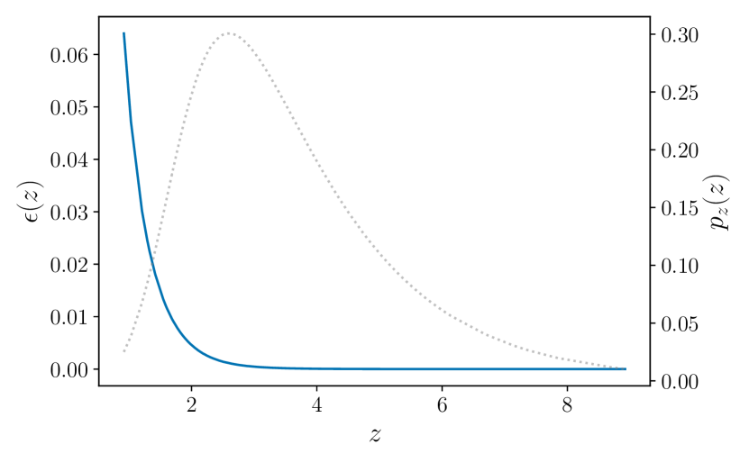
Figure 11 shows how depends on the redshift . We see that decreases as we go higher in . However, the contribution of to the selection function integral is weighted by (dotted line) which peaks at for the particular merger-rate density model and lens model we used in the calculation (cf. Sec. III).
We can employ the same Monte Carlo integration technique to evaluate the outer integral over . Suppose we have samples of , then we can approximate the entire integral as
| (69) |
Appendix C Derivation of the arrival time probability density function under the not-lensed hypothesis
Here we give a derivation of the arrival time probability density function under the not-lensed hypothesis we used in the main text, namely
| (70) |
Given that we have observed events within the interval , if we assume that the arrival of the events follows a Poisson process with a mean rate , then we can write down the joint probability distribution of the ordered arrival times (such that ) conditioned that we have observed events as
| (71) | ||||
where the second line uses the fact that for a Poisson process one can partition the time interval into many smaller chunks where each chunk still follows the same Poisson process, and that the interarrival time follows an exponential distribution. The factor is due to the requirement that there is no event between . Note that there are exactly combinations of unordered arrival times that would lead to the same ordered times. Therefore the joint probability distribution of the unordered arrival times is simply
| (72) |
Note that we are interested in the probability distribution of the time delay between arbitrary two events among these events. If we consider the unordered set of arrival times, without loss of generality we can assume that the arrival times corresponding to the two events are and respectively. The marginalization over is trivial since the joint probability density does not depend on , and the marginalized density is just
| (73) |
Note that since , this probability distribution is simply two uniform distributions multiplied together, i.e.
| (74) |
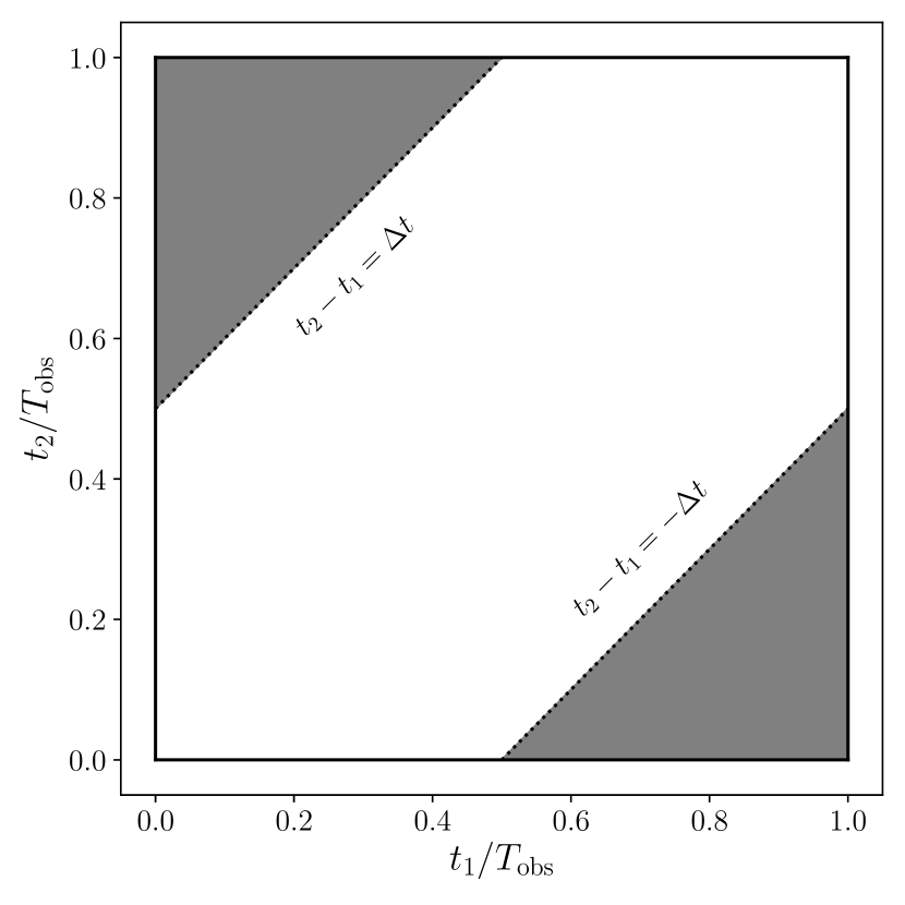
Let us define a new variable . The cumulative distribution function can be found using simple coordinate geometry by noting that the support of the joint distribution of forms a square of length (see Fig. 12). If we normalize the length by , the condition that cuts out two triangles of area from the unit square. Therefore,
| (75) | ||||
The desired probability density is a triangular distribution, i.e.,
| (76) | ||||
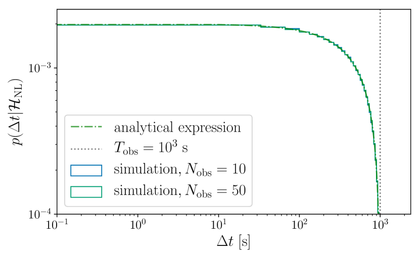
where the distribution is independent of and . This can be checked against simulations. Figure 13 shows two histograms of from simulations with and respectively. We can see that the distributions for these two cases are indeed the same, and are well described by Eq. (70).
Appendix D Derivation of the poor-man’s prior on the relative magnification
Here we will derive the poor-man’s prior on the relative magnification we used in the main text, namely
| (77) |
if we assume that the absolute magnification follows the probability distribution
| (78) |
where .
Note that the probability distribution of the ratio of two random variables can be found by evaluating the integral
| (79) | ||||
We can divide the integral into two cases; when and when . For the former case, the condition that is trivially satisfied. Therefore when , the lower limit of the integral is simply and the integral is just
| (80) | ||||
For the latter case, for the integral to not vanish. Therefore, the lower limit of the integral becomes instead, and
| (81) | ||||
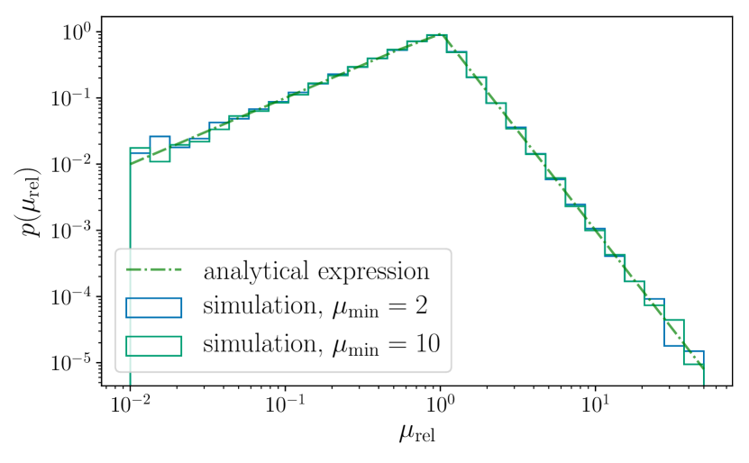
Note that this poor-man’s prior for does not depend on the value of . Again, it can be checked against simulations. Figure 14 shows the results of two simulations, assuming that and respectively. We see that the poor-man’s prior for is indeed independent of the value of the minimum value of the absolute magnification .
References
- Schneider et al. [1992] P. Schneider, J. Ehlers, and E. E. Falco, Gravitational Lenses, XIV, 560 pp. 112 figs.. Springer-Verlag Berlin Heidelberg New York. Also Astronomy and Astrophysics Library (1992) p. 112.
- Oguri [2019] M. Oguri, Strong gravitational lensing of explosive transients, Rept. Prog. Phys. 82, 126901 (2019), arXiv:1907.06830 [astro-ph.CO] .
- Takahashi and Nakamura [2003] R. Takahashi and T. Nakamura, Wave effects in gravitational lensing of gravitational waves from chirping binaries, Astrophys. J. 595, 1039 (2003), arXiv:astro-ph/0305055 .
- Dai and Venumadhav [2017] L. Dai and T. Venumadhav, On the waveforms of gravitationally lensed gravitational waves, (2017), arXiv:1702.04724 [gr-qc] .
- Ezquiaga et al. [2020] J. M. Ezquiaga, D. E. Holz, W. Hu, M. Lagos, and R. M. Wald, Phase effects from strong gravitational lensing of gravitational waves, (2020), arXiv:2008.12814 [gr-qc] .
- Ng et al. [2018] K. K. Y. Ng, K. W. K. Wong, T. Broadhurst, and T. G. F. Li, Precise LIGO Lensing Rate Predictions for Binary Black Holes, Phys. Rev. D 97, 023012 (2018), arXiv:1703.06319 [astro-ph.CO] .
- Aasi et al. [2015] J. Aasi et al. (LIGO Scientific), Advanced LIGO, Class. Quant. Grav. 32, 074001 (2015), arXiv:1411.4547 [gr-qc] .
- Acernese et al. [2015] F. Acernese et al. (VIRGO), Advanced Virgo: a second-generation interferometric gravitational wave detector, Class. Quant. Grav. 32, 024001 (2015), arXiv:1408.3978 [gr-qc] .
- Oguri [2018] M. Oguri, Effect of gravitational lensing on the distribution of gravitational waves from distant binary black hole mergers, Mon. Not. Roy. Astron. Soc. 480, 3842 (2018), arXiv:1807.02584 [astro-ph.CO] .
- Li et al. [2018] S.-S. Li, S. Mao, Y. Zhao, and Y. Lu, Gravitational lensing of gravitational waves: A statistical perspective, Mon. Not. Roy. Astron. Soc. 476, 2220 (2018), arXiv:1802.05089 [astro-ph.CO] .
- Buscicchio et al. [2020] R. Buscicchio, C. J. Moore, G. Pratten, P. Schmidt, M. Bianconi, and A. Vecchio, Constraining the lensing of binary black holes from their stochastic background, Phys. Rev. Lett. 125, 141102 (2020), arXiv:2006.04516 [astro-ph.CO] .
- Mukherjee et al. [2021] S. Mukherjee, T. Broadhurst, J. M. Diego, J. Silk, and G. F. Smoot, Inferring the lensing rate of LIGO-Virgo sources from the stochastic gravitational wave background, Mon. Not. Roy. Astron. Soc. 501, 2451 (2021), arXiv:2006.03064 [astro-ph.CO] .
- Hannuksela et al. [2019] O. A. Hannuksela, K. Haris, K. K. Y. Ng, S. Kumar, A. K. Mehta, D. Keitel, T. G. F. Li, and P. Ajith, Search for gravitational lensing signatures in LIGO-Virgo binary black hole events, Astrophys. J. Lett. 874, L2 (2019), arXiv:1901.02674 [gr-qc] .
- Dai et al. [2020] L. Dai, B. Zackay, T. Venumadhav, J. Roulet, and M. Zaldarriaga, Search for Lensed Gravitational Waves Including Morse Phase Information: An Intriguing Candidate in O2, (2020), arXiv:2007.12709 [astro-ph.HE] .
- Liu et al. [2021] X. Liu, I. M. Hernandez, and J. Creighton, Identifying strong gravitational-wave lensing during the second observing run of Advanced LIGO and Advanced Virgo, Astrophys. J. 908, 97 (2021), arXiv:2009.06539 [astro-ph.HE] .
- Broadhurst et al. [2019] T. Broadhurst, J. M. Diego, and I. Smoot, George F., Twin LIGO/Virgo Detections of a Viable Gravitationally-Lensed Black Hole Merger, arXiv e-prints , arXiv:1901.03190 (2019), arXiv:1901.03190 [astro-ph.CO] .
- Messick et al. [2017] C. Messick et al., Analysis Framework for the Prompt Discovery of Compact Binary Mergers in Gravitational-wave Data, Phys. Rev. D 95, 042001 (2017), arXiv:1604.04324 [astro-ph.IM] .
- Sachdev et al. [2019] S. Sachdev et al., The GstLAL Search Analysis Methods for Compact Binary Mergers in Advanced LIGO’s Second and Advanced Virgo’s First Observing Runs, (2019), arXiv:1901.08580 [gr-qc] .
- Usman et al. [2016] S. A. Usman et al., The PyCBC search for gravitational waves from compact binary coalescence, Class. Quant. Grav. 33, 215004 (2016), arXiv:1508.02357 [gr-qc] .
- Li et al. [2019] A. K. Y. Li, R. K. L. Lo, S. Sachdev, C. L. Chan, E. T. Lin, T. G. F. Li, and A. J. Weinstein, Finding diamonds in the rough: Targeted Sub-threshold Search for Strongly-lensed Gravitational-wave Events, (2019), arXiv:1904.06020 [gr-qc] .
- McIsaac et al. [2020] C. McIsaac, D. Keitel, T. Collett, I. Harry, S. Mozzon, O. Edy, and D. Bacon, Search for strongly lensed counterpart images of binary black hole mergers in the first two LIGO observing runs, Phys. Rev. D 102, 084031 (2020), arXiv:1912.05389 [gr-qc] .
- Haris et al. [2018] K. Haris, A. K. Mehta, S. Kumar, T. Venumadhav, and P. Ajith, Identifying strongly lensed gravitational wave signals from binary black hole mergers, (2018), arXiv:1807.07062 [gr-qc] .
- Ade et al. [2016] P. A. R. Ade et al. (Planck), Planck 2015 results. XIII. Cosmological parameters, Astron. Astrophys. 594, A13 (2016), arXiv:1502.01589 [astro-ph.CO] .
- Abbott et al. [2019] B. P. Abbott et al. (LIGO Scientific, Virgo), Binary Black Hole Population Properties Inferred from the First and Second Observing Runs of Advanced LIGO and Advanced Virgo, Astrophys. J. Lett. 882, L24 (2019), arXiv:1811.12940 [astro-ph.HE] .
- Abbott et al. [2020a] R. Abbott et al. (LIGO Scientific, Virgo), Population Properties of Compact Objects from the Second LIGO-Virgo Gravitational-Wave Transient Catalog, (2020a), arXiv:2010.14533 [astro-ph.HE] .
- Singer et al. [2019] L. P. Singer, D. A. Goldstein, and J. S. Bloom, The Two LIGO/Virgo Binary Black Hole Mergers on 2019 August 28 Were Not Strongly Lensed, (2019), arXiv:1910.03601 [astro-ph.CO] .
- Hou et al. [2019] S. Hou, X.-L. Fan, and Z.-H. Zhu, Gravitational Lensing of Gravitational Waves: Rotation of Polarization Plane, Phys. Rev. D 100, 064028 (2019), arXiv:1907.07486 [gr-qc] .
- Mandel et al. [2019] I. Mandel, W. M. Farr, and J. R. Gair, Extracting distribution parameters from multiple uncertain observations with selection biases, Mon. Not. Roy. Astron. Soc. 486, 1086 (2019), arXiv:1809.02063 [physics.data-an] .
- Ghosh et al. [2016] A. Ghosh, W. Del Pozzo, and P. Ajith, Estimating parameters of binary black holes from gravitational-wave observations of their inspiral, merger and ringdown, Phys. Rev. D 94, 104070 (2016), arXiv:1505.05607 [gr-qc] .
- Skilling [2004] J. Skilling, Nested Sampling, in Bayesian Inference and Maximum Entropy Methods in Science and Engineering: 24th International Workshop on Bayesian Inference and Maximum Entropy Methods in Science and Engineering, American Institute of Physics Conference Series, Vol. 735, edited by R. Fischer, R. Preuss, and U. V. Toussaint (2004) pp. 395–405.
- Belczynski et al. [2017] K. Belczynski, T. Ryu, R. Perna, E. Berti, T. L. Tanaka, and T. Bulik, On the likelihood of detecting gravitational waves from Population III compact object binaries, Mon. Not. Roy. Astron. Soc. 471, 4702 (2017), arXiv:1612.01524 [astro-ph.HE] .
- Liu [1994] J. S. Liu, The collapsed gibbs sampler in bayesian computations with applications to a gene regulation problem, Journal of the American Statistical Association 89, 958 (1994).
- Pratten et al. [2020] G. Pratten et al., Let’s twist again: computationally efficient models for the dominant and sub-dominant harmonic modes of precessing binary black holes, (2020), arXiv:2004.06503 [gr-qc] .
- Ashton et al. [2019] G. Ashton et al., BILBY: A user-friendly Bayesian inference library for gravitational-wave astronomy, Astrophys. J. Suppl. 241, 27 (2019), arXiv:1811.02042 [astro-ph.IM] .
- Smith et al. [2020] R. J. E. Smith, G. Ashton, A. Vajpeyi, and C. Talbot, Massively parallel Bayesian inference for transient gravitational-wave astronomy, Mon. Not. Roy. Astron. Soc. 498, 4492 (2020), arXiv:1909.11873 [gr-qc] .
- Speagle [2020] J. S. Speagle, dynesty: a dynamic nested sampling package for estimating Bayesian posteriors and evidences, Mon. Not. Roy. Astron. Soc. 493, 3132 (2020), arXiv:1904.02180 [astro-ph.IM] .
- Mateu-Lucena et al. [2022] M. Mateu-Lucena, S. Husa, M. Colleoni, H. Estellés, C. García-Quirós, D. Keitel, M. d. L. Planas, and A. Ramos-Buades, Parameter estimation with the current generation of phenomenological waveform models applied to the black hole mergers of GWTC-1, Mon. Not. Roy. Astron. Soc. 517, 2403 (2022), arXiv:2105.05960 [gr-qc] .
- bil [2020] Bilby: A user-friendly bayesian inference library, https://git.ligo.org/lscsoft/bilby/-/tree/1.0.2 (2020).
- pbi [2020] parallel_bilby: A python package to run gravitational wave inference analyses on multiple cores of a machine using their message passing interface, https://git.ligo.org/lscsoft/parallel_bilby/-/tree/0.1.5 (2020).
- Speagle et al. [2019] J. Speagle, K. Barbary, G. Ashton, J. Buchner, B. Cook, J. Guillochon, A. A. Ramos, abonaca, P. Cubillos, Ilya, D. Lang, B. Johnson, jtmendel, T. Daylan, R. Angus, P. Cargile, M. Pitkin, J. Leja, D. Goldstein, D. Foreman-Mackey, C. Talbot, and C. Deil, joshspeagle/dynesty: Version 1.0, https://doi.org/10.5281/zenodo.3461261 (2019).
- han [2021] hanabi: Hierarchical bayesian analysis on lensed gw signals using bilby, https://github.com/ricokaloklo/hanabi/tree/0.3.1 (2021).
- [42] Advanced LIGO anticipated sensitivity curves, https://dcc.ligo.org/LIGO-T1800044/public.
- Turner et al. [1984] E. L. Turner, J. P. Ostriker, and I. Gott, J. R., The statistics of gravitational lenses : the distributions of image angular separations and lens redshifts., Astrophys. J. 284, 1 (1984).
- Gerosa et al. [2020] D. Gerosa, G. Pratten, and A. Vecchio, Gravitational-wave selection effects using neural-network classifiers, Phys. Rev. D 102, 103020 (2020), arXiv:2007.06585 [astro-ph.HE] .
- Wang et al. [2021] Y. Wang, R. K. L. Lo, A. K. Y. Li, and Y. Chen, Identifying Type-II Strongly-Lensed Gravitational-Wave Images in Third-Generation Gravitational-Wave Detectors, (2021), arXiv:2101.08264 [gr-qc] .
- Seto [2004] N. Seto, Strong gravitational lensing and localization of merging massive black hole binaries with LISA, Phys. Rev. D 69, 022002 (2004), arXiv:astro-ph/0305605 .
- Hannuksela et al. [2020] O. A. Hannuksela, T. E. Collett, M. Çalışkan, and T. G. F. Li, Localizing merging black holes with sub-arcsecond precision using gravitational-wave lensing, Mon. Not. Roy. Astron. Soc. 498, 3395 (2020), arXiv:2004.13811 [astro-ph.HE] .
- Pang et al. [2020] P. T. H. Pang, O. A. Hannuksela, T. Dietrich, G. Pagano, and I. W. Harry, Lensed or not lensed: Determining lensing magnifications for binary neutron star mergers from a single detection 10.1093/mnras/staa1430 (2020), arXiv:2002.04893 [astro-ph.HE] .
- Abbott et al. [2020b] R. Abbott et al. (LIGO Scientific, Virgo), Properties and Astrophysical Implications of the 150 M⊙ Binary Black Hole Merger GW190521, Astrophys. J. Lett. 900, L13 (2020b), arXiv:2009.01190 [astro-ph.HE] .
- Goyal et al. [2021] S. Goyal, K. Haris, A. K. Mehta, and P. Ajith, Testing the nature of gravitational-wave polarizations using strongly lensed signals, Phys. Rev. D 103, 024038 (2021), arXiv:2008.07060 [gr-qc] .
- Stevenson et al. [2017] S. Stevenson, C. P. L. Berry, and I. Mandel, Hierarchical analysis of gravitational-wave measurements of binary black hole spin–orbit misalignments, Mon. Not. Roy. Astron. Soc. 471, 2801 (2017), arXiv:1703.06873 [astro-ph.HE] .
- Nakamura et al. [2016] T. Nakamura et al., Pre-DECIGO can get the smoking gun to decide the astrophysical or cosmological origin of GW150914-like binary black holes, PTEP 2016, 093E01 (2016), arXiv:1607.00897 [astro-ph.HE] .
- Koushiappas and Loeb [2017] S. M. Koushiappas and A. Loeb, Maximum redshift of gravitational wave merger events, Phys. Rev. Lett. 119, 221104 (2017), arXiv:1708.07380 [astro-ph.CO] .
- Foreman-Mackey [2016] D. Foreman-Mackey, corner.py: Scatterplot matrices in python, The Journal of Open Source Software 1, 24 (2016).
- Tiwari [2018] V. Tiwari, Estimation of the Sensitive Volume for Gravitational-wave Source Populations Using Weighted Monte Carlo Integration, Class. Quant. Grav. 35, 145009 (2018), arXiv:1712.00482 [astro-ph.HE] .
- Farr [2019] W. M. Farr, Accuracy Requirements for Empirically Measured Selection Functions, Research Notes of the American Astronomical Society 3, 66 (2019), arXiv:1904.10879 [astro-ph.IM] .
- Chen et al. [2017] H.-Y. Chen, R. Essick, S. Vitale, D. E. Holz, and E. Katsavounidis, Observational Selection Effects with Ground-based Gravitational Wave Detectors, Astrophys. J. 835, 31 (2017), arXiv:1608.00164 [astro-ph.HE] .