Adaptive efficient robust sequential analysis for autoregressive big data models ††thanks: This research was supported by RSF, project no 20-61-47043 (National Research Tomsk State University, Russia).
Abstract
In this paper we consider high dimension models based on dependent observations defined through autoregressive processes. For such models we develop an adaptive efficient estimation method via the robust sequential model selection procedures. To this end, firstly, using the Van Trees inequality, we obtain a sharp lower bound for robust risks in an explicit form given by the famous Pinsker constant (see in [21, 20] for details). It should be noted, that for such models this constant is calculated for the first time. Then, using the weighted least square method and sharp non asymptotic oracle inequalities from [4] we provide the efficiency property in the minimax sense for the proposed estimation procedure, i.e. we establish, that the upper bound for its risk coincides with the obtained lower bound. It should be emphasized that this property is obtained without using sparse conditions and in the adaptive setting when the parameter dimension and model regularity are unknown.
MSC: primary 62G08, secondary 62G05
Keywords: Autoregressive big data models; Robust estimation; Sequential estimation; Model selection; Sharp oracle inequality; Pinsker constant; Asymptotic efficiency.
1 Introduction
1.1 Problem and motivations
We study the observations model defined for through the following difference equation
| (1.1) |
where the initial value is a non random known constant, are known linearly independent functions, are fixed known constants and are i.i.d. unobservable random variables with an unknown density distribution from some functional class which will be specified later.
The problem is to estimate the unknown parameters in the high dimension setting, i.e. when the number of parameters more than the number of observations, i.e. . Usually, in these cases one uses one of two methods: Lasso algorithm or the Dantzig selector method (see, for example, [14] and the references therein). It should be emphasized, that in the papers devoted to big data models the number of parameters must be known and, moreover, usually it is assumed sparse conditions to provide optimality properties. Therefore, unfortunately, these methods can’t be used to estimate, for example, the number of parameters . To overcome these restrictions in this paper similar to the approach proposed in [13] we study this problem in the nonparametric setting, i.e. we embed the observations (1.1) in the general model defined as
| (1.2) |
where is unknown function. The nonparametric setting allows to consider the models (1.1) with unknown or even with . Note that the case when the number of parameters is unknown is one of challenging problems in the signal and image processing theory (see, for example, [7, 5]). So, now the problem is to estimate the function on the basis of the observations (1.2) under the condition that the noise distribution is unknown and belongs to some functional class . There is a number of papers which consider these models (see, for example, [6, 8, 18] and the references therein). Firstly, minimax estimation problems for the model (1.2) has been treated in [2, 19] in the nonadaptive case, i.e. for the known regularity of the function . Then, in [1] and [3] it is proposed to use the sequential analysis for the adaptive pointwise estimation problem, i.e. in the case when the Hölder regularity is unknown. Moreover, it turned out that only the sequential methods can provide the adaptive estimation for autoregressive models. That is why in this paper we use the adaptive sequential procedures from [4] for the efficient estimation, which we study for the quadratic risks
where is an estimator of based on observations and is the expectation with respect to the distribution law of the process given the distribution density and the function . Moreover, taking into account that is unknown, we use the robust risk defined as
| (1.3) |
where is a family of the distributions defined in Section 2.
1.2 Main tools
To estimate the function in model (1.2) we make use of the model selection procedures proposed in [4]. These procedures are based on the family of the optimal poin-twise truncated sequential estimators from [3] for which sharp oracle inequalities are obtained through the model selection method developed in [9]. In this paper, on the basis of these inequalities we show that the model selection procedures are efficient in the adaptive setting for the robust quadratic risk (1.3). To this end, first of all, we have to study the sharp lower bound for the these risks, i.e. we have to provide the best potential accuracy estimation for the model (1.2) which usually for quadratic risks is given by the Pinsker constant (see, for example, in [21, 20]). To do this we use the approach proposed in [10, 11] based on the Van-Trees inequality. It turns out that for the model (1.2) the Pinsker constant equals to the minimal quadratic risk value for the filtration signal problem studied in [21] multiplied by the coefficient obtained through the integration of the optimal pointwise estimation risk on the interval . This is a new result in the nonparametric estimation theory for the statistical models with dependent observations. Then, using the oracle inequality from [4] and the weight least square estimation method we show that, for the model selection procedure the upper bound asymptotically coincides with the obtained Pinsker constant without using the regularity properties of the unknown functions, i.e. it is efficient in adaptive setting with respect to the robust risk (1.3).
1.3 Organization of the paper
The paper is organized as follows. In Section 2 we construct the sequential pointwise estimation procedures which allows us to pass from the autoregression model to the corresponding regression model, then in Section 3 we develop the model selection method. We announce the main results in Section 4. In Section 5 we present Monte - Carlo results which numerically illustrate the behavior of the proposed model selection procedures. In Section 6 we show the Van-Trees inequality for the model (1.2). We obtain the lower bound for the robust risk in Section 7 and in Section 8 we get the upper bound for the robust risk of the constructed sequential estimator. In Appendix we give the all auxiliary tools.
2 Sequential point-wise estimation method
To estimate the function in the model (1.2) on the interval we use the kernel sequentail estimators proposed in [3] at the points defined as
| (2.1) |
where is an integer valued function of , i.e. , such that as . Note that in this case the kernel estimator has the following form
where is a kernel function and is a bandwidth. As is shown in [2] to provide an efficient point wise estimation, the kernel function must be chosen as the indicator of the interval , i.e. . This means that we can rewrite the estimator (2) as
| (2.2) |
where and , is the integer part of , and . To use the model selection method from [4] we need to obtain the uncorrelated stochastic terms in the kernel estimators for the function at the points (2.1), i.e. one needs to use the disjoint observations sets . To this end it suffices to choose for which for all the bounds , i.e. we set
| (2.3) |
Note that the main difficulty is that the kernel estimator is the non linear function of the observations due to the random denominator. To control this denominator we need to assume conditions providing the stability properties for the model (1.2). To obtain the stable (uniformly with respect to the function ) model (1.2), we assume that for some fixed and the unknown function belongs to the -stability set introduced in [3] as
| (2.4) |
where is the Banach space of continuously differentiable functions and . As is shown in [4]
Therefore, to replace the denominator in (2.2) with its limit we need firstly preliminary estimate the function . We estimate it as
| (2.5) |
where for some . Indeed, we can not use this estimator directly to replace the random denominator since in general it can be closed to one. By this reason we use its projection into the interval in , i.e. and . Finally, omitting some technical details, we will replace the denominator (2.2) with the threshold defined as
| (2.6) |
It should be noted that is a function the observations . To replace the random denominator in (2.2) with the we use the sequential estimation method through the following stopping time
| (2.7) |
where . It is clear that a.s. Now we define the sequential estimator as
| (2.8) |
where and the correcting coefficient is defined as
| (2.9) |
To study robust properties of this sequential procedure similarly to [3] we assume that in the model (1.2) the i.i.d. random variables have a density (with respect to the Lebesgue measure) from the functional class defined as
| (2.10) |
where is some fixed parameter, which may be a function of the number observation , i.e. , such that for any
| (2.11) |
Note that the Gaussian density belongs to .
Now we can formulate the following proposition from [4] (Theorem 3.1).
Proposition 2.1.
For any
| (2.12) |
where as such that for any .
Now we set
| (2.13) |
In Theorem 3.2 from [4] it is shown that the probability of goes to zero uniformly more rapid than any power of the observations number , which is formulated in the next proposition.
Proposition 2.2.
For any the probability of the set satisfies the following asymptotic equality
In view of this proposition we can negligible the set . So, using the estimators (2.13) on the set we obtain the discrete time regression model
| (2.14) |
in which
where
and . Note that the random variables (see Lemma A.2 in [4]), for any and are such that
| (2.15) |
where , and is a fixed constant. Note that
| (2.16) |
where
Remark 1.
It should be summarized that we construct the sequential pointwise procedure (2.7) – (2.8) in two steps. First, we preliminary estimate the function in (2.5) on the observations and through this estimator we replace the random denominator in (2.8) with the threshold in the second step when we construct the estimation procedure on the basis of the observations . It should be noted also that in the deviation (2.14) the main term has a martingale form and the second one, as it is shown in [4], is asymptotically small. It should be emphasized that namely these properties allow us to develop effective estimation methods.
3 Model selection
Now to estimate the function we use the sequential model selection procedure from [4] for the regression (2.14). To this end, first we choose the trigonometric basis in , i.e.
| (3.1) |
where the function for even and for odd , and . Moreover, we choose the odd number of regression points (2.1), for example, . Then the functions are orthonormal for the empirical inner product, i.e.
| (3.2) |
It is clear that, the function can be represented as
| (3.3) |
We define the estimators for the coefficients as
| (3.4) |
From (2.14) we obtain immediately the following regression on the set
| (3.5) |
where
Through the Bounyakovskii-Cauchy-Schwarz we get that
| (3.6) |
where . Note here, that as it is shown in [4] (Theorem 3.3) for any
| (3.7) |
To construct the model selection procedure we use weighted least squares estimators defined as
| (3.8) |
where the weight vector belongs to some finite set , the prime denotes the transposition. Denote by the cardinal number of the set , for which we impose the following condition.
Assume that the number of the weight vectors as a function of , i.e. , such that for any the sequence as .
To choose a weight vector in (3.8) we will use the following risk
| (3.9) |
Using (3.3) and (3.8) it can be represented as
| (3.10) |
Since the coefficients are unknown we can’t minimize this risk directly to obtain an optimal weight vector. To modify it we set
| (3.11) |
Note here that in view of (2.16) - (3.2) the last term can be estimated as
| (3.12) |
Now, we modify the risk (3.10) as
| (3.13) |
where the coefficient will be chosen later and the penalty term is
| (3.14) |
Now using (3.13) we define the sequential model selection procedure as
| (3.15) |
To study the efficiency property we specify the weight coefficients as it is proposed, for example, in [10]. First, for some introduce the two dimensional grid to adapt to the unknown parameters (regularity and size) of the Sobolev ball, i.e. we set
| (3.16) |
where . We assume that both parameters and are functions of , i.e. and , such that
| (3.17) |
for any . One can take, for example, for
| (3.18) |
where is some fixed integer number. For each , we introduce the weight sequence with the elements
| (3.19) |
and
Here, and are such that , and as . In this case we set . Note, that these weight coefficients are used in [16, 17] for continuous time regression models to show the asymptotic efficiency. It will be noted that in this case the cardinal of the set is . It is clear that the properties (3.17) imply the condition . In [4] we showed the following result.
Theorem 3.1.
4 Main results
First, to study the minimax properties for the estimation problem for the model (1.2) we need to introduce some functional class. To this end for any fixed and we set
| (4.1) |
where , are the trigonometric Fourier coefficients in , i.e. and is the trigonometric basis defined in (3.1). It is clear that we can represent this functional class as the Sobolev ball
Now, for this set we define the normalizing coefficients
and
| (4.2) |
It is well known that in regression models with the functions the minimax convergence rate is (see, for example, [10, 15] and the references therein). Our goal in this paper is to show the same property for the non parametric auto-regressive models (1.2). First we have to obtain a lower bound for the risk (1.3) over all possible estimators , i.e. any measurable function of the observations .
Theorem 4.1.
Now to study the procedure (3.15) we have to add some condition on the penalty coefficient which provides sufficiently small penalty term in (3.13).
: Assume that the parameter is a function of , i.e. such that and for any .
Theorem 4.2.
Corollary 4.1.
Remark 3.
Note that the limit equalities (4.4) and (4.5) imply that the function is the minimal value of the normalized asymptotic quadratic robust risk, i.e. the Pinsker constant in this case. We remind that the coefficient is the well known Pinsker constant for the ”signal+standard white noise” model obtained in [21]. Therefore, the Pinsker constant for the model (1.2) is represented by the Pinsker constant for the ”signal+white noise” model in which the noise intensity is given by the function (4.2).
Now we assume that in the model (1.2) the functions are orthonormal in , i.e. . We use the estimators (3.8) to estimate the parameters as and . Then, similarly we use the selection model procedure (3.15) as
| (4.6) |
It is clear, that in this case and .
Note, that Theorem 3.1 implies that the estimator (4.6) is optimal in the sharp oracle inequality sense which is established in the following theorem.
Theorem 4.3.
Note now, that Theorems 4.1 and 4.2 imply the efficiency property for the estimate (4.6) based on the model selection procedure (3.15) constructed with the penalty threshold satisfying the condition .
Theorem 4.4.
Then the estimate (4.6) is asymptotically efficient, i.e.
and
| (4.7) |
where is the set estimators for based on the observations .
5 Monte - Carlo simulations
In this section we present the numeric results obtained through the Python soft for the model (1.2) in which are i.i.d. random variables and , i.e. and . In this case we simulate the model selection procedure (3.15) with the weights (3.19) in which , , . Moreover, the parameters and are chosen as
and . First we study the model (1.2) with and then for the function
In the model selection procedures we use points in (2.1).
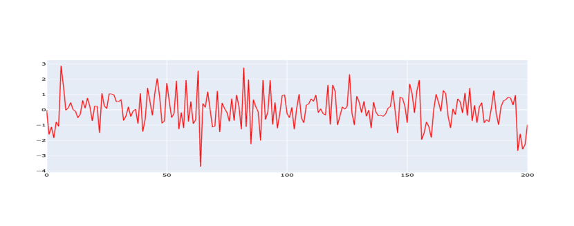
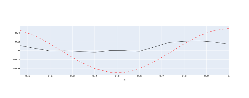
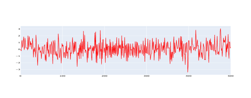
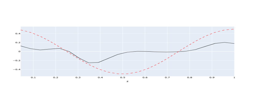
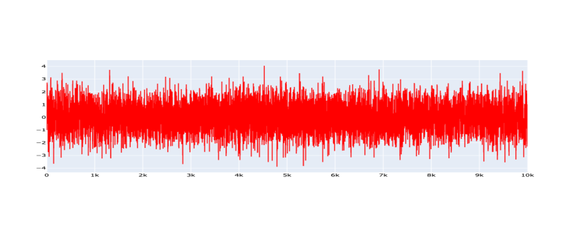
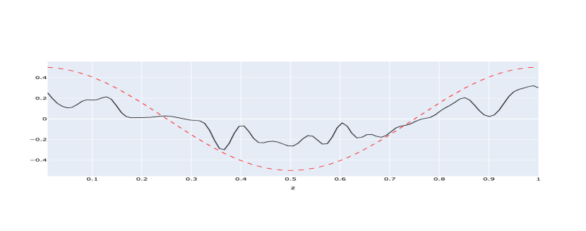
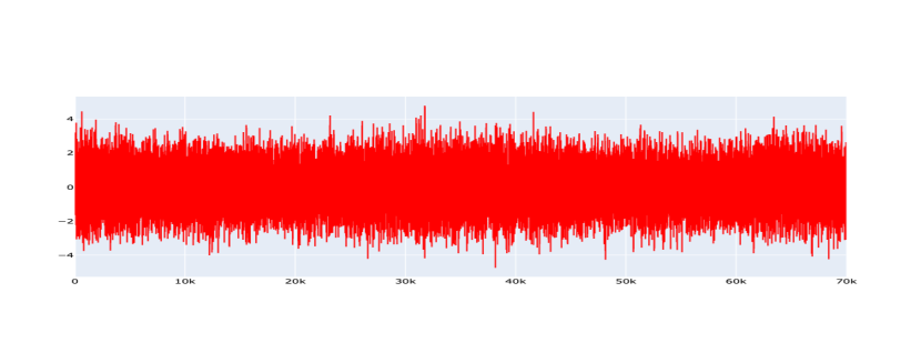
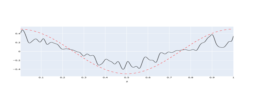
Figures 1–4 show the behavior of the function and its estimators by the model selection procedure (3.15) depending on the observations number . In the figures (a) the observations are given and in (b) the red dotted is the regression function and the black full line is its estimator at the points (2.1). Then we calculate the empiric risks as
| (5.1) |
where the expectation is taken as an average over replications, i.e.
We use also the relative risk
| (5.2) |
The tables below give the values for the sample risks (5.1) and (5.2) for different numbers of observations .
| n | ||
|---|---|---|
| 200 | 0.135 | 0.98 |
| 500 | 0.0893 | 0.624 |
| 10000 | 0.043 | 0.362 |
| 70000 | 0.03523 | 0.281 |
| n | ||
|---|---|---|
| 200 | 0.0821 | 5.685 |
| 500 | 0.0386 | 2.623 |
| 10000 | 0.0071 | 0.516 |
| 70000 | 0.0067 | 0.419 |
Remark 5.
From numerical simulations of the procedure (3.15) with various observation durations and for the different functions we may conclude that the quality of the estimation improves as the number of observations increases.
6 The van Trees inequality
In this section we consider the nonparametric autoregressive model (1.2) with the gaussian i.i.d. random variable and the parametric linear function , i.e.
| (6.1) |
We assume that the functions are orthogonal with respect to the scalar product (3.2). Let now be the distribution in of the observations in the model (1.2) with the function (6.1) and be the distribution in of the gaussian vector . In this case the Radon - Nykodim density is given as
| (6.2) |
Let be a prior distribution density on for the parameter of the following form , where is a some probability density in with continuously derivative for which the Fisher information is finite, i.e.
| (6.3) |
Let be a continuously differentiable function such that
| (6.4) |
where .
For any -measurable integrable function we denote
| (6.5) |
Let be the field generated by the observations (1.2), i.e. . Now we study the Gaussian the model (1.2) with the function (6.1).
Lemma 6.1.
For any -measurable square integrable function and for any , the mean square accuracy of the function with respect to the distribution (6.5) can be estimated from below as
| (6.6) |
where and .
Proof. First, for any we set
Taking into account the condition (6.4) and integrating by parts we get
Now by the Bouniakovskii-Cauchy-Schwarz inequality we obtain the following lower bound for the quadratic risk . To study the denominator in this inequality note that in view of the representation (6.2)
Therefore, for each ,
and
Using the equality
we get . Hence Lemma 6.1. ∎
7 Lower bound
First, taking into account that the gaussian density belongs to the class (2.10), we get . Now, according to the general lower bounds methods (see, for example, in [10]) one needs to estimate this risk from below by some bayesian risk and, then to apply the van Trees inequlity. To define the bayesian risk we need to choose a prior distribution on . To this end, first for any vector , we set
| (7.1) |
where is the trigonometric basis defined in (3.1). We will choose a prior distribution on the basis of the optimal coefficients in (7.1) (see, for example, in [20, 21]) providing asymptotically the maximal valuer for the risk over . So, we choose it as the distribution in of the random vector defined by its components as
| (7.2) |
where are i.i.d. random variables with the continuously differentiable density defined in Lemma A.1 with and ,
To choose the number of the terms in (7.1) one needs to keep this function in , i.e. one needs to provide for arbitrary fixed the following property
| (7.3) |
To do this we set
| (7.4) |
where and
It is clear that almost sure the function (7.1) can be bounded as
| (7.5) |
where . Note, that as for . Therefore, for sufficiently large the function (7.1) belongs to the class (2.4). Now, , we denote by its projection in onto the ball , i.e. . Since , then for we have , where . Therefore, for large
| (7.6) |
where and . Note that as . Using the distribution we introduce the following Bayes risk as
| (7.7) |
Now taking into account that , we get
| (7.8) |
and . Note here that this term is studied In Lemma A.3. Moreover, note also that for any we get and . Therefore, from Lemma 6.1 with it follows, that for any and any measurable random variable
where and . Therefore, the Bayes risk can be estimated from below as
where
| (7.9) |
Note here, that in view of Lemmas A.1 and A.2 for any and sufficiently large we have and , therefore,
Using here that , we obtain for sufficiently large
Therefore, taking into account this in (7.8) we conclude through the definition (7.4) and Lemma A.3, that for any and
Taking here limit as and we come to the Theorem 4.1. ∎
8 Upper bound
We start with the estimation problem for the functions from with known parameters , and defined in (4.2). In this case we use the estimator from family (3.19)
| (8.1) |
where , and . Note that for sufficiently large , the parameter belongs to the set (3.16). In this section we study the risk for the estimator (8.1). To this end we need firstly to analyse the asymptotic behavior of the sequance
| (8.2) |
Proposition 8.1.
The sequence is bounded from above
Proof. First, note that . This implies directly that
| (8.3) |
where and . Moreover, note that
and , where
Remind, that and . Note now, that Lemma A.5 and Lemma A.6 yield
and
i.e. , where
and . Note, that
where . It is clear that . Therefore, from (8.3) it follows that
Next note, that for any and for sufficiently large
i.e.
Next, since as , we get directly that
Finally, taking into account, that , we obtain Proposition 8.1. ∎
Theorem 8.1.
The estimator constructed on the trigonometric basis satisfies the following asymptotic upper bound
| (8.4) |
Proof. We denote and . Now we recall that the Fourier coefficients on the set
Therefore, on the set we can represent the empiric squared error as
where . Now for any
where is defined in (3.6). Therefore,
By the same way we get
Thus, on the set we find that for any
where is defined in (8.2) and
| (8.5) |
We recall that the variance is defined in (4.2). In view of Lemma A.7
where is given in (2.16). Moreover, using that , we get
Therefore, Proposition 2.2 yields
| (8.6) |
Now, the property (3.7) Proposition 8.1 and Lemma A.8 imply the inequality (8.4). Hence Theorem 8.1. ∎
Acknowledgements. The last author was partially supported by RFBR and CNRS (research project number 20 - 51 - 15001).
A Appendix
A.1 Properties of the prior distribution 7.2
In this section we study properties of the distribution used in (7.7).
Lemma A.1.
For any there exists a continuously differentiable probability density on with the support on the interval , i.e. for and for , such that for any the integral and, moreover, and as .
Proof. First we set . It is clear that this function is infinitely times continuously differentiable, such that for , for and . Now for we set . Using here the properties of the function we can obtain directly that for , for , for and for . Moreover, it is clear that the derivative . Note here that for some . Now through the Bunyakovsky - Cauchy - Schwartz inequality we get that . Now we set , where the Gaussian density, It is clear that is the the continuously differentiable probability density with the support such that for any the integral and , for . Moreover, the Fisher information can be represented as
where, taking into account that for ,
Therefore, as . Hence Lemma A.1. ∎
Lemma A.2.
The term (7.9) is such that .
Proof. First, note that for . Therefore, and due to (7.5) we obtain that for any for which
Since, , we get Lemma A.2. ∎
Lemma A.3.
The term in (7.8) is such that for any and .
Proof. First note, that taking into account in the definition of term in (7.8), that , we get that . Therefore, to show this lemma it suffices to check that for any . To do this note, that the definition of in (7.6) implies and . So, it suffices to show that
| (A.1) |
Indeed, first note, that the definition (7.2) through Lemma A.1 and the property (7.3) imply directly
Setting now and , we get for large that for . Now the correlation inequality from [12] and the bound imply that for any there exists some constant for which
i.e. the expectation as and, therefore, as for any . This implies (A.1) and, hence Lemma A.3. ∎
A.2 Properties of the trigonometric basis.
First we need the following lemma from [17].
Lemma A.4.
Let be an absolutely continuous function, with and be a piecewise constant function of a form where are some constants. Then for any the function satisfies the following inequalities
Lemma A.5.
For any the trigonometric Fourier coefficients for the functions from the class with satisfy, for any , the following inequality .
Proof. First we represent the function as and , i.e. and, therefore, we get . Lemma A.4 with implies . Using here that for , we obtain that and
| (A.2) |
Hence Lemma A.5 ∎
Lemma A.6.
For any and the coefficients of functions from the class with satisfy, for any , the inequality .
A.3 Technical lemmas
Lemma A.7.
Proof. Using the definition of in (3.5) and the bounds (2.16), we get
Now, the orthonormality property (3.2) implies this lemma. ∎
Lemma A.8.
For the sequence (8.5) the following limit property holds true
Proof. First of all, note that, using the definition of in (3.11), we obtain
where and . Therefore, we can represent the expectation of as
where ,
Note now, that using Proposition 2.12 and the dominated convergence theorem in the definition (2.6) we obtain that
Taking into account that for the functions from the class (2.4) their derivatives are uniformly bounded, we can deduce that
i.e. . Therefore, taking into account that
we obtain that
| (A.3) |
where
References
- [1] Arkoun, O (2011): Sequential Adaptive Estimators in Nonparametric Autoregressive Models, Sequential Analysis 30: 228-246.
- [2] Arkoun, O. and Pergamenchtchikov, S. (2008) : Nonparametric Estimation for an Autoregressive Model, Tomsk State University Journal of Mathematics and Mechanics. 2: 20-30.
- [3] Arkoun, O. and Pergamenchtchikov, S. (2016) : Sequential Robust Estimation for Nonparametric Autoregressive Models. - Sequential Analysis, 2016, 35 (4), 489 – 515
- [4] Arkoun, O. , Brua, J.-Y. and Pergamenchtchikov, S. (2019) Sequential Model Selection Method for Nonparametric Autoregression. - Sequential Analysis, 38 (4), 437 - 460.
- [5] Bayisa, F.L., Zhou, Z., Cronie, O. and Yu, J. (2019) Adaptive algorithm for sparse signal recovery. Digital Signal Processing, 87, 10 – 18.
- [6] Belitser, E. (2000) Recursive Estimation of a Drifted Autoregressive Parameter, The Annals of Statistics 26: 860-870.
- [7] Beltaief, S., Chernoyarov, O. and Pergamenchtchikov, S. (2020) Model selection for the robust efficient signal processing observed with small Levy noise. - Ann Inst Stat Math., 72, 1205 - 1235.
- [8] Fan, J. and Zhang, W. (2008) Statistical Methods with Varying Coefficient Models. -Statistics and Its Interface, 1, 179–195.
- [9] Galtchouk, L.I. and Pergamenshchikov, S.M. (2009) Sharp non-asymptotic oracle inequalities for nonparametric heteroscedastic regression models. Journal of Nonparametric Statistics, 21, 1-16.
- [10] Galtchouk, L.I. and Pergamenshchikov, S.M. (2009) Adaptive asymptotically efficient estimation in heteroscedastic nonparametric regression. Journal of the Korean Statistical Society, 38 (4), 305 - 322.
- [11] Galtchouk, L. and Pergamenshchikov, S. (2011) : Adaptive Sequential Estimation for Ergodic Diffusion Processes in Quadratic Metric, Journal of Nonparametric Statistics 23: 255-285.
- [12] Galtchouk, L. and Pergamenshchikov, S. (2013) Uniform concentration inequality for ergodic diffusion processes observe at discrete times, Stochastic processes and their applications, 123, 91 - 109.
- [13] Galtchouk, L. and Pergamenshchikov, S. (2021) Adaptive efficient analysis for big data ergodic diffusion models. - Statistical inference for stochastic processes, 2021, DOI 10.1007/s11203-021-09241-9, http://link.springer.com/article/10.1007/s11203-021-09241-9
- [14] Hasttie, T., Friedman, J. and Tibshirani, R. The Elements of Statistical Leaning. Data Mining, Inference and Prediction.// Second Edition, Springer, Springer series in Statistics, - 2008, 764 p.
- [15] Konev, V.V. and Pergamenshchikov, S. M. Non-parametric estimation in a semimartingale regression model. Part 2. Robust asymptotic efficiency. Tomsk State University Journal of Mathematics and Mechanics, 2009, 4(8), 31-45.
- [16] V.V. Konev and S.M. Pergamenshchikov. Efficient robust nonparametric estimation in a semimartingale regression model. Ann. Inst. Henri Poincaré Probab. Stat., 48 (4), 2012, 1217–1244.
- [17] V.V. Konev and S.M. Pergamenshchikov. Robust model selection for a semimartingale continuous time regression from discrete data. Stochastic processes and their applications, 125, 2015, 294 – 326.
- [18] Luo, X. H., Yang, Z. H. and Zhou, Y. (2009) : Nonparametric Estimation of the Production Function with Time-Varying Elasticity Coefficients, Systems Engineering-Theory & Practice 29: 144-149.
- [19] Moulines, E., Priouret, P. and Roueff, F. (2005) On Recursive Estimation for Time Varying Autoregressive Processes, The Annals of Statistics 33, 2610 – 2654.
- [20] Pchelintsev, E., Pergamenshchikov, S.M. and Povzun, M. (2021) Efficient estimation methods for non-Gaussian regression models in continuous time. - Annals of the Institute of Statistical Mathematics, DOI 10.1007/s10463-021-00790-7,
- [21] Pinsker, M.S. (1981) Optimal filtration of square integrable signals in gaussian noise. - Problems Inform. Transmission, 17, 120-133.