SILVERRUSH X: Machine Learning-Aided Selection of $9$,$318$ LAEs
at $z=2.2$, $3.3$, $4.9$, $5.7$, $6.6$, and $7.0$ from the HSC SSP and CHORUS Survey Data

Abstract

We present a new catalog of $9$,$318$ Ly$\alpha$ emitter (LAE) candidates at $z=2.2$, $3.3$, $4.9$, $5.7$, $6.6$, and $7.0$ that are photometrically selected by the SILVERRUSH program with a machine learning technique from large area (up to $25.0$ deg²) imaging data with six narrowband filters taken by the Subaru Strategic Program with Hyper Suprime-Cam (HSC SSP) and a Subaru intensive program, Cosmic HydrOgen Reionization Unveiled with Subaru (CHORUS). We construct a convolutional neural network that distinguishes between real LAEs and contaminants with a completeness of $94$% and a contamination rate of $1$%, enabling us to efficiently remove contaminants from the photometrically selected LAE candidates. We confirm that our LAE catalogs include $177$ LAEs that have been spectroscopically identified in our SILVERRUSH programs and previous studies, ensuring the validity of our machine learning selection. In addition, we find that the object-matching rates between our LAE catalogs and our previous results are $\simeq 80$–$100$% at bright NB magnitudes of $\lesssim 24$ mag. We also confirm that the surface number densities of our LAE candidates are consistent with previous results. Our LAE catalogs will be made public on our project webpage.

1. Introduction

Large panoramic surveys over cosmological volumes such as the Subaru Hyper Suprime-Cam (HSC) survey (Aihara et al. 2018) and the Dark Energy Survey (DES; Abbott et al. 2018) are providing massive multiwavelength data sets for unprecedentedly large numbers of astronomical sources. Such big data are key to understanding galaxy formation and evolution, allowing us to investigate statistical properties of high-$z$ galaxies (Ono et al. 2018; Harikane et al. 2018a; Ouchi et al. 2018; Konno et al. 2018; Stevans et al. 2018; Guarnieri et al. 2019: Adams et al. 2020; Moutard et al. 2020) and pinpoint very rare interesting structures and objects such as galaxy overdensities (Toshikawa et al. 2018; Ito et al. 2019; Higuchi et al. 2019; Harikane et al. 2019), very luminous Ly$\alpha$ emitters (LAEs) and Ly$\alpha$ blobs (Shibuya et al. 2018a; Songaila et al. 2018; Kikuta et al. 2019; Zhang et al. 2020; Taylor et al. 2020; see also the recent review of Ouchi et al. 2020). In the near future, further significant progress is expected to be made by next generation telescopes such as Vera C. Rubin Observatory (VRO), Euclid, and the Nancy Grace Roman Space Telescope.

One of the fundamental problems in analyzing such big data is that the amount of obtained data can be too large to handle. For example, in our last LAE search based on the HSC survey data (Shibuya et al. 2018a), we have conducted visual inspection of the photometrically selected candidates to remove contaminants in a similar way to previous studies (e.g., Ouchi et al. 2008; Ouchi et al. 2010). However, due to the very large area of the HSC survey, it took about two person-months to complete the visual inspection task, suggesting that it could be almost impossible to obtain scientific results in a timely manner by taking advantage of big data obtained by future large surveys with reasonable human and computational resources.

Recently, advances in machine learning techniques have revolutionized the field of image recognition and shown a wide variety of successful applications (Lecun et al. 2015). Because observational astronomical studies also utilize imaging data sets, machine learning methods are becoming prevalent in astronomy (Baron 2019), such as for source detections (Vafaei Sadr et al. 2019; Burke et al. 2019), galaxy morphological classifications and measurements (Dieleman et al. 2015; Huertas-Company et al. 2015; Domínguez Sánchez et al. 2018; Martin et al. 2020; Hausen & Robertson 2020; Cheng et al. 2020; Ghosh et al. 2020; Tohill et al. 2020; see also, Tadaki et al. 2020), photometric redshift estimates (Hoyle 2016; D’Isanto & Polsterer 2018; Pasquet et al. 2019), gravitationally lensed image searches (Hezaveh et al. 2017; Lanusse et al. 2018; Schaefer et al. 2018; Jacobs et al. 2019; He et al. 2020; Li et al. 2020; Canameras et al. 2020; Huang et al. 2020b), extremely metal-poor galaxy searches (Kojima et al. 2020), transient source detections (Morii et al. 2016; Parfeni et al. 2020), light curve classifications (Charnock & Moss 2017; Pasquet-Itam & Pasquet 2018; Shallue & Vanderburg 2018; Takahashi et al. 2020), optical depth reconstructions of Ly$\alpha$ forest absorption (Huang et al. 2020a), stellar spectrum classifications (Traven et al. 2017; Buder et al. 2018), and anomaly detections (Giles & Walkowicz 2019; Ichinohe & Yamada 2019; Čotar et al. 2021; D’Addona et al. 2020; Lochner & Bassett 2020). Convolutional neural networks (CNNs) are frequently adopted for image classification problems as well as various other computer vision related tasks such as image segmentation and object recognition. Similar to other machine learning techniques, CNNs are trained to learn how to directly extract representative features from imaging data and to make intelligent judgements or estimates.

In this work, we apply machine learning in the form of CNNs to image classifications between high-$z$ LAEs and contaminants to efficiently construct samples of LAE candidates at $z=2.2$, $3.3$, $4.9$, $5.7$, $6.6$, and $7.0$ based on the HSC imaging data obtained by the Subaru Strategic Program (HSC SSP; Aihara et al. 2018; see also Miyazaki et al. 2012; Miyazaki et al. 2018; Komiyama et al. 2018; Kawanomoto et al. 2018; Furusawa et al. 2018) as well as a Subaru intensive program, Cosmic HydrOgen Reionization Unveiled with Subaru (CHORUS; Inoue et al. 2020; see also Itoh et al. 2018; Zhang et al. 2020). This paper is included in a series of papers on LAEs based on the HSC SSP survey, Systematic Identification of LAEs for Visible Exploration and Reionization Research Using Subaru HSC (SILVERRUSH; Ouchi et al. 2018; Shibuya et al. 2018a; Shibuya et al. 2018b; Konno et al. 2018; Harikane et al. 2018b; Inoue et al. 2018; Higuchi et al. 2019; Harikane et al. 2019; Kakuma et al. 2019; H. Goto et al. in prep.; S. Kikuchihara et al. in prep.). The major improvements from our previous work are the advent of a new narrowband (NB) filter, $NB387$, and deeper depths of broadband (BB) data, as well as a compilation of results from four NB data of $NB387$, $NB527$, $NB718$, and $NB973$ taken by the CHORUS program. Our new SILVERRUSH LAE catalogs based on new HSC SSP and CHORUS data with the aid of the machine learning technique will be made public on our project webpage.

This paper is organized as follows. In Section 2, we describe our HSC SSP and CHORUS data, and photometric selections for high-$z$ LAE candidates based on multiwavelength catalogs with HSC NB and BB data. Our machine learning selection is described in Section 3, and the constructed LAE catalogs and their statistical properties are presented in Section 4. A summary is described in Section 5. In this paper, we use magnitudes in the AB system (Oke & Gunn 1983) and assume a flat universe with $\Omega_{\rm m}=0.3$, $\Omega_{\Lambda}=0.7$, and $H_{0}=70$ km s^-1 Mpc^-1.

Table 1Summary of the NB filter properties used in this study

Filter	$\lambda_{\rm c}$	FWHM	$z_{{\rm Ly}\alpha}$	References
	(Å)	(Å)
(1)	(2)	(3)	(4)	(5)
$NB387$	3863	55	$2.178\pm 0.023$	Aihara et al. (2018); Inoue et al. (2020)
$NB527$	5260	79	$3.327\pm 0.032$	Inoue et al. (2020)
$NB718$	7171	111	$4.899\pm 0.046$	Inoue et al. (2020)
$NB816$	8177	113	$5.726\pm 0.046$	Aihara et al. (2018); Ouchi et al. (2018)
$NB921$	9215	135	$6.580\pm 0.056$	Aihara et al. (2018); Ouchi et al. (2018)
$NB973$	9712	112	$6.989\pm 0.046$	Inoue et al. (2020)

Note. — (1) Filter name. (2) Central wavelength in Å. (3) FWHM of the transmission function in Å. (4) Redshift range of Ly$\alpha$ emission that can be probed within the NB FWHM. (5) Papers that present the detailed properties of the NBs.

Figure 1.— Transmission curves of the NB and BB filters. The blue, green, yellow, orange, magenta, and red curves correspond to the $NB387$, $NB527$, $NB718$, $NB816$, $NB921$, and $NB973$ filters, respectively. The black curves represent the $g$-, $r$-, $i$-, $z$-, and $y$-band filters from left to right. These transmission values are obtained by multiplying the area-weighted mean values of the filters by the quantum efficiency of CCDs, the transmittance values of the dewar window and the primary focus unit of HSC, and the reflectivity of the primary mirror.

Table 2HSC SSP Survey data used in this study

Field	Area ($NB387$)	Area ($NB816$)	Area ($NB921$)	$NB387$	$NB816$	$NB921$	$g$	$r$	$i$	$z$	$y$
	(deg2)	(deg2)	(deg2)	(mag)	(mag)	(mag)	(mag)	(mag)	(mag)	(mag)	(mag)
(1)	(2)	(3)	(4)	(5)	(6)	(7)	(8)	(9)	(10)	(11)	(12)
UD-SXDS	—	2.278	2.278	—	25.61	25.31	26.83	26.42	26.24	25.74	24.96
UD-COSMOS	—	2.261	2.278	—	25.75	25.48	26.93	26.52	26.50	26.30	25.60
D-SXDS	4.928	4.789	—	24.29	25.16	—	26.65	26.03	25.62	25.51	24.27
D-COSMOS	7.296	—	6.198	24.71	—	25.07	26.58	26.32	26.23	25.90	25.02
D-ELAIS-N1	—	7.145	7.215	—	25.23	25.02	26.63	26.16	26.00	25.57	24.68
D-DEEP2-3	6.802	7.197	6.980	24.25	25.26	24.86	26.51	26.10	25.81	25.52	24.80
Total	19.03	23.67	24.95

Note. — (1) Field name. (2)–(4) Effective area in deg². (5)–(12) Typical $5\sigma$ limiting magnitudes measured with $2\farcs 0$ diameter circular apertures in $NB387$, $NB816$, $NB921$, $g$, $r$, $i$, $z$, and $y$. For $NB387$, we consider the 0.45 mag offset described in Section 2. The standard deviation is typically $\simeq 0.5$ mag, if the edge of the field of view, where few objects are selected, is also taken into account. It is much smaller if we focus on more central regions. Note that the limiting magnitudes are measured for different aperture sizes when compared to those in Table 1 of Shibuya et al. (2018a).

Table 3CHORUS NB data used in this study

Field	Area ($NB387$)	Area ($NB527$)	Area ($NB718$)	Area ($NB973$)	$NB387$	$NB527$	$NB718$	$NB973$
	(deg2)	(deg2)	(deg2)	(deg2)	(mag)	(mag)	(mag)	(mag)
(1)	(2)	(3)	(4)	(5)	(6)	(7)	(8)	(9)
UD-COSMOS	1.561	1.613	1.575	1.603	25.67	26.39	25.59	24.90

Note. — (1) Field name. (2)–(5) Effective area in deg² after removing the masked regions (Inoue et al. 2020). (6)–(9) Typical $5\sigma$ limiting magnitudes measured with $2\farcs 0$ diameter circular apertures in $NB387$, $NB527$, $NB718$, and $NB973$. For $NB387$, we consider the 0.45 mag offset described in Section 2. See Figure 4 of Inoue et al. (2020) for the spatial variations of the limiting magnitudes.

2. Data and Photometric Selection

Figure 2.— BB$-$NB color diagrams for photometric selections of LAEs at $z=2.2$ (top) and $z=3.3$ (bottom): $r-NB387$ vs. $g-NB387$ (top left); $z-NB387$ vs. $i-NB387$ (top right); $r-NB527$ vs. $g-NB527$ (bottom left); $z-NB527$ vs. $i-NB527$ (bottom right). The solid curve corresponds to the color track of a redshifted galaxy SED with Ly$\alpha$ EW of $20$Å in the rest frame. We use the Bruzual & Charlot (2003) stellar population synthesis model with a Salpeter (1955) initial mass function (IMF) and adopt a $30$ Myr simple stellar population whose UV continuum slope is sufficiently blue, consistent with previous observational results (e.g., Stark et al. 2010; Santos et al. 2020). We add a Ly$\alpha$ emission and take into account the Madau (1995) prescription of the intergalactic medium (IGM) absorption. The SED is redshifted from $z=0.0$ to $z=3.50$ with a step of $\Delta z=0.01$. The symbols on these model tracks correspond to $z=2.14$ (filled triangles), $z=2.16$ (filled squares), $z=2.18$ (filled circles), $z=2.20$ (open squares), and $z=2.22$ (open triangles) in the top panels, and $z=3.28$ (filled triangles), $z=3.30$ (filled squares), $z=3.32$ (filled circles), $z=3.34$ (open squares), and $z=3.36$ (open triangles) in the bottom panels. The dashed lines denote the color criteria to photometrically select our LAE candidates. Note that the model track slightly changes with Ly$\alpha$ EW only in the two color diagram of $g-NB527$ vs. $r-NB527$. In the other diagrams, the model tracks with larger EW values overlap and extend to the upper right, since there is no wavelength overlap between NB and BB.

Figure 3.— BB$-$NB colors as a function of redshift for $z=4.9$, $z=5.7$, $z=6.6$, and $z=7.0$ LAEs: $ri-NB718$, $i-NB816$, $z-NB921$, and $y-NB973$ from left to right. The solid blue curves denote the track of the redshifted galaxy SED with Ly$\alpha$ EW of $20$Å in the rest frame, which is the same as that of Figure 2. The solid black, green, orange, and red curves are the same as the solid blue curve but for other Ly$\alpha$ EWs of $10$, $30$, $50$, and $150$Å in the rest frame, respectively, as presented in the legend in the left panel. The horizontal dashed lines denote the color criteria to photometrically select our LAE candidates.

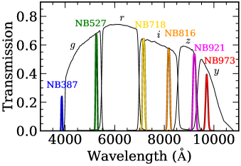
We use data products of the on-going HSC SSP survey that were obtained between 2014 March and 2018 January (Aihara et al. 2019). Specifically, we use the internal data release of S18A, which is basically identical to the version of Public Data Release 2. The HSC survey consists of three layers: Ultra-deep (UD), Deep (D), and Wide. Among these three layers, the UD (D) layer is covered with two (three) NB filters of ($NB387$,) $NB816$, and $NB921$ that are designed to efficiently identify emission line sources, as well as five BB filters of $g$, $r$, $i$, $z$, and $y$. Thus, in this study, we use the HSC SSP data for the UD and D layers. The basic properties of the $NB387$, $NB816$, and $NB921$ filters are summarized in Table 1 and their transmission curves are shown in Figure 1. The UD layer has two fields: UD-SXDS and UD-COSMOS. The D layer consists of four fields: D-SXDS, D-COSMOS, D-ELAIS-N1, and D-DEEP2-3. The observed areas with the NBs are shown in Table 2.

In addition, we use HSC NB data taken by the CHORUS program between 2017 January and 2018 March (Inoue et al. 2020). In the CHORUS program, the COSMOS field in the UD layer is covered with four NB filters of $NB387$, $NB527$, $NB718$, and $NB973$, as well as an intermediate filter, $IB945$. In this study, we use these NB data to efficiently select LAE candidates. The basic properties of these NB filters are also presented in Table 1 and their transmission curves are also shown in Figure 1. The effective survey area of the NB data are summarized in Table 3.

These HSC data were reduced with hscPipe 6.7, which exploits codes from the VRO software pipeline (Bosch et al. 2018; see also Axelrod et al. 2010; Jurić et al. 2017; Ivezić et al. 2019). Full details of the HSC SSP survey and the CHORUS program such as observations and data reduction are described in Aihara et al. (2019) (see also Aihara et al. 2018) and Inoue et al. (2020), respectively. Note that we correct a systematic offset in the zero-point magnitude of the $NB387$ data by subtracting $0.45$ mag, following the previous studies (Liang et al. 2020; Inoue et al. 2020).

To photometrically select LAE candidates based on NB color excess features, we create multiwavelength catalogs of NB-detected sources in the HSC data. We use the $NB387$, $NB527$, $NB718$, $NB816$, $NB921$, and $NB973$ data as detection images for $z=2.2$, $3.3$, $4.9$, $5.7$, $6.6$, and $7.0$ LAE candidate selections, respectively. First we smooth the HSC BB images and each NB image for each redshift sample with Gaussian kernels so that their point spread function (PSF) full width at half maximums (FWHMs) are matched to the largest ones. For this purpose, for the HSC SSP data, we download a PSF image for each filter for each $\simeq 12^{\prime}\times 12^{\prime}$ patch from the PSF Picker website and smooth the multiwavelength images patch by patch. For the CHORUS data, we create a PSF image for each filter by stacking $\sim 200$ point-source-like bright objects detected in the UD-COSMOS field. Typical PSF FWHMs of the smoothed HSC images are about 0$\farcs$8–1$\farcs$1. We then run SExtractor (Bertin & Arnouts 1996) in the dual image mode for the PSF-matched images, to make multiwavelength catalogs. The main reason why we use SExtractor instead of hscPipe to construct multiwavelength catalogs for our photometric selections of LAEs is because it is easier for us to change the priority of the detection filters. We set DETECT_MINAREA to 5 and DETECT_THRESH to 2.0. We adopt MAG_AUTO as total magnitudes, while we use $2\farcs 0$ diameter circular aperture magnitudes to measure colors of detected sources. The limiting magnitudes within $2\farcs 0$ diameter apertures for the HSC SSP and CHORUS data are summarized in Tables 2 and 3, respectively.

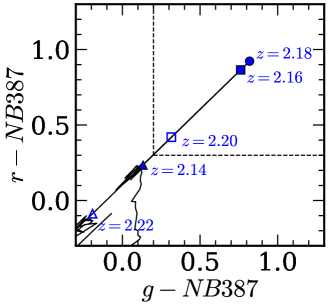
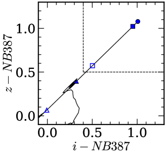
From the multiwavelength catalogs, we photometrically select LAE candidates at $z=2.2$, $3.3$, $4.9$, $5.7$, $6.6$, and $7.0$ that show clear NB excesses compared to BB magnitudes. First, we select sources with signal-to-noise ratio (S/N) $>5$ within $2\farcs 0$ diameter apertures in the corresponding NB data for each redshift sample. We then select LAE candidates by using their NB and BB magnitudes and colors. For $z=2.2$ LAEs, we adopt

$$g-NB387 \geq 0.2,$$ (1)

$$r-NB387 \geq 0.3,$$ (2)

$$i-NB387 \geq 0.4,$$ (3)

$$z-NB387 \geq 0.5,$$ (4)

and for $z=3.3$ LAEs, we apply the following criteria

$$g-NB527 \geq 0.9,$$ (5)

$$r-NB527 \geq 0.3,$$ (6)

$$i-NB527 \geq 0.4,$$ (7)

$$z-NB527 \geq 0.5,$$ (8)

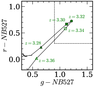
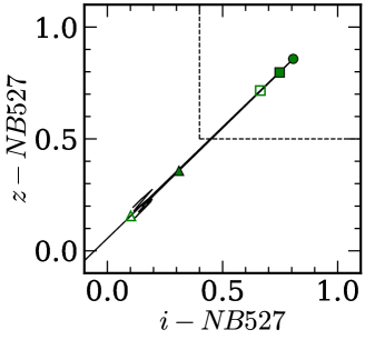
by considering the NB$-$BB colors of spectral energy distributions (SEDs) of young galaxies with strong Ly$\alpha$ emission (see also Nakajima et al. 2012; Konno et al. 2016) as presented in Figure 2. For $z=4.9$ LAEs, we apply these criteria,

$$ri-NB718>0.7\,\,\mathrm{and}\,\,r-i>0.8\,\,\mathrm{and}$$ (9)

$$ri-NB718>\left(ri-NB718\right)_{3\sigma}\,\,\mathrm{and}\,\,g>g_{2\sigma},$$ (10)

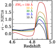
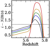
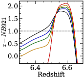
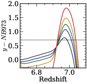
where $ri$ is calculated by the linear combination of the fluxes in the $r$ band, $f_{r}$, and the fluxes in the $i$ band, $f_{i}$, following $f_{ri}=0.3f_{r}+0.7f_{i}$ (Zhang et al. 2020). The $2\sigma$ and $3\sigma$ subscripts denote $2\sigma$ and $3\sigma$ limiting magnitudes, respectively. We use the $ri$ magnitude, because the wavelength of the $NB718$ band is located between the $r$ and $i$ bands (Figure 1). The expected $ri-NB718$ color as a function of redshift for LAEs with Ly$\alpha$ equivalent width (EW) in the rest frame of $EW_{0}=20$Å is presented in Figure 3. Similar NB excess selections have been adopted in previous studies (e.g., Ouchi et al. 2003; Shimasaku et al. 2003; Shimasaku et al. 2004). For $z=5.7$ and $z=6.6$ LAEs, we adopt

$$i-NB816\geq 1.2,$$ (11)

and

$$z-NB921\geq 1.0$$ (12)

respectively, following Shibuya et al. (2018a). For $z=7.0$ LAEs, we adopt

$$\left[\left(y<y_{3\sigma}\,\,\mathrm{and}\,\,y-NB973>0.7\right)\,\,\mathrm{or}\,\,y>y_{3\sigma}\right]\,\,\mathrm{and}$$ (13)

$$\left[\left(z<z_{3\sigma}\,\,\mathrm{and}\,\,z-y>2\right)\,\,\mathrm{or}\,\,z>z_{3\sigma}\right]\,\,\mathrm{and}$$ (14)

$$\hskip 3.00003ptg>g_{2\sigma}\,\,\mathrm{and}\,\,r>r_{2\sigma}\,\,\mathrm{and}\,\,i>i_{2\sigma},$$ (15)

which are almost the same as those used in Itoh et al. (2018) and Zhang et al. (2020). Their expected BB$-$NB colors as a function of redshift are also shown in Figure 3. These BB$-$NB selection criteria correspond to Ly$\alpha$ EW limits of $EW_{0}\gtrsim 10$–$20$Å in the rest frame (see also Zhang et al. 2020; Shibuya et al. 2018a; Itoh et al. 2018). The specific Ly$\alpha$ EW limit for each redshift sample is summarized in Section 4 together with previous studies for comparisons of the LAE number counts.

Table 4Layout of our CNN

ID	Type	Size	$n$	Activation
(1)	(2)	(3)	(4)	(5)
1	input	$50\times 50$	—	—
2	convolutional	$5\times 5$	$32$	ReLU
3	convolutional	$5\times 5$	$64$	ReLU
4	dropout (0.5)	—	—	—
5	average pooling	$2\times 2$	—	—
6	convolutional	$5\times 5$	$128$	ReLU
7	convolutional	$5\times 5$	$128$	ReLU
8	dropout (0.5)	—	—	—
9	average pooling	$2\times 2$	—	—
10	dense	$256$	—	ReLU
11	dropout (0.5)	—	—	—
12	dense	$8$	—	softmax

Note. — (1) ID of the layers. (2) Type of the layers. (3) Size of the data or the filters. (4) Number of the filters. (5) Activation function adopted in the layers.

Table 5Classes in the output layer of our CNN

Class	Comment
1	LAEs with S/N = 3–4
2	LAEs with S/N = 4–10
3	LAEs with S/N = 10–30
4	LAEs with S/N = 30–200
5	bright satellite trails
6	faint satellite trails
7	randomly selected noise images
8	randomly selected noise images with positive sky residuals

Figure 4.— Example images of Classes 1–8. Classes 1, 2, 3, and 4 are simulated LAEs with S/Ns of $3$–$4$, $4$–$10$, $10$–$30$, and $30$–$200$, respectively. Classes 5 and 6 are bright and faint satellite trails, respectively. Classes 7 and 8 are randomly selected noise images without and with positive sky residuals, respectively. The size of the images is $\simeq 10^{\prime\prime}\times 10^{\prime\prime}$.

Figure 5.— Results of the 8-label classification for the test data. The $x$-axis is the predicted class. The colored solid lines represent the fractions of classified images, and their colors denote the true classes (red: Class 1; light pink: Class 2; magenta: Class 3; red: Class 4; cyan: Class 5; blue: Class 6; green: Class 7; dark green: Class 8).

Figure 6.— Confusion matrix. In the top panel, Classes 1–4 (5–8) of the true labels are classified as positive (negative). For the predicted labels, we classify sources as positive if they show a high score of being an LAE (for details, see Section 3.2). The numbers in the cells denote true positives (TP), false negatives (FN), false positives (FP), and true negatives (TN). In the best case scenario, the confusion matrix has non-zero elements only in its diagonal cells and zero elements in the others. The bottom panel is the same as the top panel, except that positive for the true labels corresponds to simulated LAEs with S/N$>5$.

Figure 7.— Completeness as a function of input S/N with corresponding input magnitude where the $5\sigma$ limiting magnitude is about $25.0$ mag on the upper $x$-axis. The vertical dotted line denotes S/N $=5$.

The numbers of LAE candidates that are photometrically selected with the color criteria described above are $258670$ for $z=2.2$ LAEs, $13937$ for $z=3.3$ LAEs, $2544$ for $z=4.9$ LAEs, $186386$ for $z=5.7$ LAEs, $176129$ for $z=6.6$ LAEs, and $21789$ for $z=7.0$ LAEs. These large numbers include many contaminants such as satellite trails and low-$z$ emission line galaxies. As mentioned in Section 1, in our previous work, Shibuya et al. (2018a) performed visual inspection for the BB and NB images of their photometrically selected 121000 LAE candidates, which took about two person-months. In this study, the number of photometrically selected LAE candidates is $258670+13937+2544+186386+176129+21789=659455$. If we scale the results of Shibuya et al. (2018a), the amount of human effort that is needed for visual inspection of all the photometrically selected LAE candidates is estimated to be about 11 person-months. In this study, we apply a machine learning technique for removal of obvious contaminants to overcome this problem. This technique allows us to significantly reduce the required human resources.

3. Machine Learning Selection

3.1. Implementation

We adopt a machine learning based selection to remove contaminants such as satellite trails and low-$z$ galaxies from the photometrically selected LAE candidate catalogs. For this purpose, we train a CNN so that it can distinguish between real LAEs, satellite trails, and noise images based on single band images. Our strategy is, with the trained CNN, to select sources as LAE candidates that are classified as real LAEs in NB probing Ly$\alpha$ emission and also classified as noise images in BB probing a wavelength range bluer than the Lyman limit (Section 4).

Table 6Number of selected LAEs

Field	$z=2.2$	$z=3.3$	$z=4.9$	$z=5.7$	$z=6.6$	$z=7.0$
(1)	(2)	(3)	(4)	(5)	(6)	(7)
UD-SXDS	—	—	—	560	75	—
UD-COSMOS	542†1	959†1	349†1	395	150	40†1
D-SXDS	850	—	—	532†3	—	—
D-COSMOS	2173†2	—	—	—	111†4	—
D-ELAIS-N1	—	—	—	409	170	—
D-DEEP2-3	844	—	—	985	174	—
Total†5	4409	959	349	2881	680	40

Note. — (1) Field name. (2)–(7) Number of selected LAEs at $z=2.2$–$7.0$.

The CNN architecture used in this study is presented in Table 4. We input a $50\times 50$ pixel (corresponding to $8\farcs 4\times 8\farcs 4$) cutout image centered on a galaxy coordinate. Our CNN consists of four convolutional layers with $5\times 5$ filters, two average pooling layers, and two fully connected layers. Although many previous studies use max pooling for image classification problems, we find that average pooling performs better for our purpose, probably because background noises in our data are relatively high compared to those in typical image classification work (see also Pasquet et al. 2019). Dropout regularization is performed after two convolutional layers to reduce the chance of overfitting by randomly dropping a half of the output neurons during training. The hidden layers use the ReLU (linear rectifier) activation function (Nair & Hinton 2010), and the output layer uses the softmax function. Because the slope of the ReLU activation function is zero for negative input values, we add $+0.2$ to the pixel counts in the input images so that most of the pixels have positive values. The output of the fully connected layer for each category is a predicted score; a higher score for a category means that the input is more likely to be classified as the category. In the output layer, we have eight classes in total, depending on their types and S/Ns (Table 5; for details, see Section 3.2). We use the Adam optimization algorithm (Kingma & Ba 2014) to minimize the cross-entropy error function over training data. The basic idea of this network architecture is motivated by previous similar studies (Huertas-Company et al. 2018; see also, M. Okura et al. in prep.). We implement this network by using the Python neural network library Keras (Chollet & others 2018) with the TensorFlow backend (Abadi et al. 2016).

3.2. Training

For the training of the CNN, we create data sets for LAEs. Because the number of spectroscopically identified LAEs is limited, we make simulated images of LAEs by using the SynPipe software (Huang et al. 2018), which utilizes GalSim v1.4 (Rowe et al. 2015) and the HSC pipeline. The simulated LAE images are generated so that they have various S/Ns of $3$–$200$ in $2\farcs 0$ diameter circular apertures. The size distribution of these simulated LAEs follows the observational results of Leclercq et al. (2017). Specifically, we create a histogram of the $r_{S_{\mathrm{cont}}}$ values presented in Table B.1 of Leclercq et al. (2017) and generate random size values that follow the distribution. We adopt a uniform distribution of Sérsic indices in the range of $1$–$3$ to consider the scatter of the measured Sérsic indices of LAEs (Shibuya et al. 2019). The SynPipe software inserts the simulated LAE images into HSC images at random positions. Although these simulated images allow the CNN to learn what most LAEs are like, it should be noted that there are also rare, extended LAEs (Ly$\alpha$ blobs) and Ly$\alpha$-emitting merging galaxies some of which may be excluded in our machine learning selection. We will check this issue in Section 4 by comparing our final LAE sample and previously spectroscopically identified LAEs. Because of the wide S/N range of the simulated LAEs, we divide them into four classes according to their S/Ns to improve the accuracy of our CNN classification. Specifically, Classes 1, 2, 3, and 4 consist of simulated LAEs with S/Ns of $3$–$4$, $4$–$10$, $10$–$30$, and $30$–$200$, respectively. The number of simulated images in each class is 12500. Their example images are shown in Figure 4.

In addition, we collect data sets for contaminants. We create two classes for satellite trails depending on their S/Ns; Classes 5 and 6 are bright and faint satellite trails that are labelled in our previous visual inspection (Shibuya et al. 2018a). Since the numbers of labelled satellite trails are limited, we augment their images by applying $90$, $180$, and $270$ degree rotations and horizontal and vertical flips. We also create two classes for null detections. Class 7 corresponds to randomly selected noise images and Class 8 is the same as Class 7 but shows positive sky residuals of $\simeq 0.1$–$0.3$. Because such noise images can be selected as LAE candidates due to noise fluctuations, these classes are also categorized as contaminants. The number of these images in each class is 12500, and their example images are presented in Figure 4. Note that, in the photometrically selected sample, there should be some contaminants that are not considered in the training data for the CNN such as cosmic rays and diffuse artifacts. Although such contaminants would not be completely excluded in this machine learning selection, we perform visual inspection to remove the remaining ones afterwards. The main advantage of this machine learning selection is that it enables us to remove many obvious contaminants automatically.

In total, we have eight classes as summarized in Table 5. We divide the data for each class into two subsets: training (80%) and test (20%). We use the training data to tune model parameters of the CNN during development, applying a five-fold cross-validation procedure. The test data are used for evaluation of the developed model performance. Note that the model performance does not depend on redshift, because the size distribution of Leclercq et al. (2017) and the Sérsic indices considering the results of Shibuya et al. (2019) are adopted to create the simulated LAE images for the training, which are sufficient to account for morphologies of most LAEs in the redshift range of $z=2.2$–$7.0$. We thus apply the trained CNN model to all the redshift samples. The differences of absolute noise values in different input images are taken into account by scaling the input images as described in Section 4.

Table 7Summary of LAE searches used in our number count comparisons

Reference	Redshift	Ly$\alpha$ $EW_{0}$ limit	$m_{{\rm NB},5\sigma}$	Area	# of LAE candidates
		(Å)	(mag)	(deg2)
(1)	(2)	(3)	(4)	(5)	(6)
Nakajima et al. (2012, 2013)	$2.2$	$30$	25.6–26.5	$1.2$†1	3169†1
Hao et al. (2018)	$2.2$	$20$–$30$	26.0†2	0.34	475
This study	$2.2$	$20$	24.3–25.7	20.6	4409
Ouchi et al. (2008)	$3.1$	$64$	25.1–25.5	1.0	356†3
This study	$3.3$	$20$	26.4	1.6	959
Ouchi et al. (2008)	$3.7$	$44$	24.6–25.2	1.0	101†3
Zhang et al. (2020)	$4.9$	$20$	26.2†4	1.6	141
This study	$4.9$	$20$	25.6	1.6	349
Ouchi et al. (2008)	$5.7$	$27$	25.9–26.1	1.0	401†3
Shibuya et al. (2018a)	$5.7$	$10$	25.2–25.7†4	13.8	1077
This study	$5.7$	$10$	25.2–25.7	23.7	2881
Ouchi et al. (2010)	$6.6$	$14$	25.6–25.8	0.90	207
Shibuya et al. (2018a)	$6.6$	$\sim 10$†5	24.9–25.6†4	21.2	1153
This study	$6.6$	$\sim 10$†5	24.9–25.5	25.0	680
Itoh et al. (2018)	$7.0$	$20$	25.0†4	3.1†6	34
This study	$7.0$	$20$	24.9	1.6	40

Note. — (1) References. (2) Redshifts. (3) Ly$\alpha$ EW limits in the rest frame. (4) $5\sigma$ limiting magnitudes in NBs measured with $2\farcs 0$ diameter circular apertures unless otherwise mentioned. (5) Effective area in deg². (6) Numbers of LAE candidates.

Table 8Fitting results of the filter transmission functions for the redshift distributions

Filter	$\alpha$	$\beta$
(1)	(2)	(3)
$NB387$	$41.64^{+11.08}_{-9.40}$	$-0.002^{+0.003}_{-0.004}$
$NB718$	$4.58^{+2.00}_{-1.57}$	$-0.030^{+0.016}_{-0.018}$
$NB816$	$32.90^{+3.70}_{-3.47}$	$-0.020^{+0.002}_{-0.003}$
$NB921$	$12.00^{+3.11}_{-2.91}$	$-0.023^{+0.014}_{-0.010}$

Note. — (1) Filter. (2)–(3) Best-fit normalization constant and shift along the $x$-axis derived from the two parameter fitting.

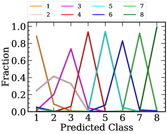
Figure 5 shows the $8$-label classification results for the test data. We classify each image into a class where a highest predicted score is obtained. All the classes show highest fractions for the true classes. In particular, Classes 1, 4, 5, 6, 7, 8 achieve high accuracies of $\gtrsim 80$–$90$% for the true classes. However, Classes 2 and 3 show relatively low accuracies, because non-negligible fractions of images in Classes 2 and 3 are classified into the other classes of LAEs with different S/Ns.

Figure 8.— Surface number density of LAEs at $z=2.2$ (top left), $z=3.3$ (top right), $z=4.9$ (middle left), $z=5.7$ (middle right), $z=6.6$ (bottom left), and $z=7.0$ (bottom right) as a function of total NB magnitude. For redshifts where multiple subfields are observed, we show the averaged results with red circles and the subfield results with black symbols. These surface number density values are not corrected for completeness. The subfield results are slightly offset for clarity.

Although we divide the input data into the eight classes in total, our interest is basically whether an object is classified as positive (i.e., LAEs) or negative (i.e., contaminants such as satellite trails and randomly selected noise images). Thus, we use the CNN as a classifier that works on the binary classification problem. We define sources as positive if they show a high score of being an LAE, satisfying $p_{1}+p_{2}+p_{3}+p_{4}>0.95$ and $p_{2}+p_{3}+p_{4}>0.5$, where $p_{i}$ denotes the score of Class $i$. Sources that do not satisfy these criteria are classified as negative ones.

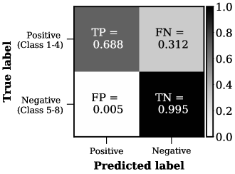
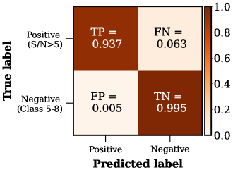
Figure 6 shows the confusion matrices for our binary classification results. For binary classification problems, confusion matrices split predictions into true positives (TPs, i.e., simulated LAEs recovered by the CNN), false positives (FPs, i.e., contaminants that are selected as LAEs by the CNN), false negatives (FNs, i.e., simulated LAEs that are not selected by the CNN), and true negatives (TNs, i.e., contaminants recovered by the CNN).

Figure 9.— Surface number density of LAEs at $z=2.2$ (top left), $z=3.3$ (top right), $z=4.9$ (middle left), $z=5.7$ (middle right), $z=6.6$ (bottom left), and $z=7.0$ (bottom right) as a function of total NB magnitude. The red circles are our results. These surface number density values are not corrected for completeness. For comparison, we also show previous results of Nakajima et al. (2012), Nakajima et al. (2013), and Hao et al. (2018) for $z=2.2$ LAEs (see also Konno et al. 2016), Ouchi et al. (2008) for $z=3.1$, $z=3.7$, and $z=5.7$ LAEs, Zhang et al. (2020) for $z=4.9$ LAEs, Ouchi et al. (2010) for $z=6.6$ LAEs, Shibuya et al. (2018a) for $z=5.7$ and $6.6$ LAEs, and Itoh et al. (2018) for $z=7.0$ LAEs. These previous results are slightly offset for clarity.

Based on the results shown in the top panel of Figure 6, the completeness of the classifier, $f_{\rm comp}$, can be obtained from

$$f_{\rm comp}=\frac{n_{\rm TP}}{n_{\rm TP}+n_{\rm FN}},$$ (16)

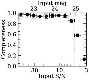
where $n_{\rm TP}$ denotes the number of true positives, and $n_{\rm FN}$ is the number of false negatives. We find that the $f_{\rm comp}$ value for the test data of the simulated LAEs in Classes 1–4 is not so high, about $69$%. This is because these classes include simulated LAEs with low S/Ns down to only $3$. Figure 7 shows the completeness as a function of input S/N. We find that the $f_{\rm comp}$ values are $\gtrsim 90$% for bright sources with input magnitudes of $\lesssim 24.5$ mag. To remove the effect from low-S/N sources, we show the confusion matrix in the bottom panel of Figure 6 where we focus on simulated LAEs with S/Ns $>5$ for the true labels. We find that the $f_{\rm comp}$ value for simulated LAEs with S/Ns $>5$ is high, $\simeq 94$%．

From the confusion matrix, we also calculate the contamination rate of the classifier, $f_{\rm cont}$,

$$f_{\rm cont}=\frac{n_{\rm FP}}{n_{\rm TP}+n_{\rm FP}},$$ (17)

where $n_{\rm FP}$ is the number of false positives. We confirm that the contamination rate is very low, only $\simeq 1$%, based on the bottom panel of Figure 6.

It should be noted that these completeness and contamination rate estimates are the results for the test data, controlling the balance of the numbers in the classes. For the actual data, these values should be different, because the number ratios between the classes are different. However, we do not rely solely on the machine learning selection for contamination removal. As described above in this section, after applying the machine learning selection, we perform visual inspection to further remove possible contaminants that are not excluded with the CNN.

4. Results: Application to the New HSC SSP and CHORUS Data

We apply the trained CNN to our photometrically selected LAE candidates prepared in Section 2 to efficiently remove contaminants such as satellite trails and low-$z$ interlopers by making use of our HSC NB and BB images.

Our machine learning selection consists of two steps. First we use the NB images of the photometrically selected LAE candidates as input data for the CNN and obtain their score for each class to select sources with a high score of being a positive (an LAE). In this process, we remove contaminants of satellite trails from the photometrically selected LAE candidates based on their morphologies in the NB images. Next, we use their BB images whose wavelength coverages are basically shorter than the Lyman limit wavelengths for targeted redshifts. We require that the candidates have $p_{7}+p_{8}>0.5$, i.e., a high score of null detection, which enables us to remove low-$z$ interlopers from the photometrically selected LAE candidates. For this purpose, we use $g$-band images for $z=4.9$ and $z=5.7$ LAEs, $g$- and $r$-band images for $z=6.6$ LAEs, and $g$-, $r$-, and $i$-band images for $z=7.0$ LAEs. We do not use BB images for $z=2.2$ and $z=3.3$ LAEs, because their Lyman limit wavelengths are still shorter than the $g$-band wavelength coverage. Note that, because the absolute value of noise is different in each band, the input NB and BB images are scaled so that the absolute noise values are comparable to those of the training data in these two steps.

After these two steps, the numbers of LAE candidates in our samples are significantly reduced. The numbers of the remaining LAE candidates at $z=2.2$, $3.3$, $4.9$, $5.7$, $6.6$, and $7.0$ are about $8000$, $2600$, $1500$, $10000$, $5000$, and $380$, which correspond to about $3$, $18$, $58$, $6$, $3$, and $2$ % of the photometrically selected LAE candidates, respectively. Although the difference of these fractions is due to the different fractions of obvious contaminants in the photometrically selected LAE candidates, which are likely to depend on the strictness of the photometric selection criteria, these low values indicate that our CNN removes a large number of contaminants in the photometrically selected LAE samples. Thanks to the CNN application, the human resources that are needed for the visual inspection are greatly reduced compared to our previous work (see Sections 2 and 3.2).

We then perform visual inspection of the NB and BB images of the LAE candidates that satisfy our machine learning selection criteria to further remove possible contaminants. Most contaminants excluded in this visual inspection process are the ones that are not considered in the training data for the CNN as expected, such as cosmic rays, diffuse artifacts, and noisy images around the edge of the survey area where the image qualities are poor. Our careful selection yields samples of 4409, 959, 349, 2881, 680, and 40 LAE candidates at $z=2.2$, $3.3$, $4.9$, $5.7$, $6.6$, and $7.0$, which correspond to about $60$, $40$, $20$, $30$, $10$, and $10$ % of the LAE candidates that satisfy the machine learning selection criteria, respectively. Some of the fractions are still not so high. However, these fractions decrease without the machine learning selection to $1.7$, $6.9$, $14$, $1.5$, $0.4$, and $0.2$% for the $z=2.2$, $3.3$, $4.9$, $5.7$, $6.6$, and $7.0$ LAE samples, respectively, which indicates a significant improvement thanks to the machine learning selection, although it also depends on the strictness of the photometric selection criteria. Note that the score of a spectroscopically confirmed spatially extended LAE, Himiko (Ouchi et al. 2009; Ouchi et al. 2013), for its NB data is slightly smaller than the criterion of $p_{1}+p_{2}+p_{3}+p_{4}>0.95$. This is probably because its morphology is significantly more extended than those adopted for the training data, although other extended LAEs such as CR7 (Sobral et al. 2015) satisfy the NB criterion. Because Himiko has already been spectroscopically confirmed, we add it to the final catalog. In addition, we notice that the score of another spectroscopically confirmed LAE, COLA-1 (Hu et al. 2016), for the BB data is higher than the criterion probably due to the presence of a foreground object at $z=2.142$ in its vicinity on the sky (Matthee et al. 2018). Because COLA-1 is also a spectroscopically confirmed LAE, it is also included in the final catalog. The number of our LAE candidates in the final catalog with each NB for each field is summarized in Table 6.

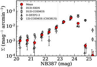
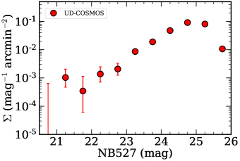
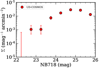
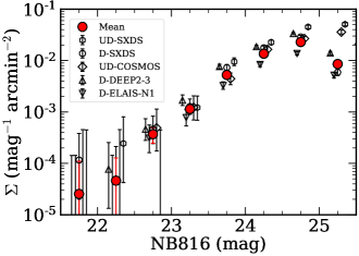
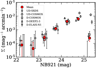
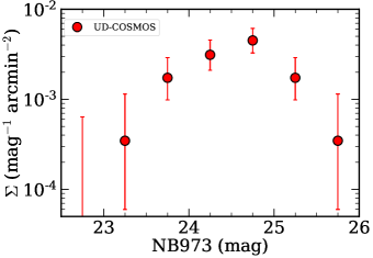
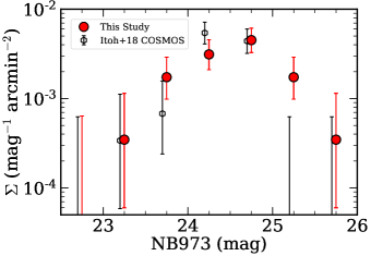
Figure 8 shows the number counts of our LAE candidates in the final catalogs at $z=2.2$, $3.3$, $4.9$, $5.7$, $6.6$, and $7.0$ as a function of total NB magnitude. To calculate the $1\sigma$ uncertainties, we take account of Poisson confidence limits (Gehrels 1986) on the number of the selected LAE candidates in each NB magnitude bin. For the LAE samples selected from the CHORUS data, we apply the masks that are provided by Inoue et al. (2020) for conservative estimates, although the number count results are mostly consistent with the results without the masks. At $z=2.2$, $5.7$, and $6.6$, we also show the number counts of the LAE candidates for the survey fields separately. We confirm that these number counts are broadly consistent with each other at each redshift.

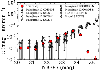
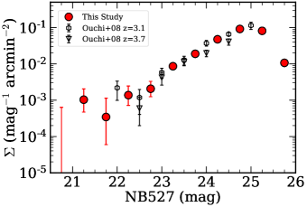
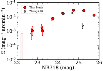
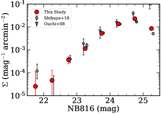
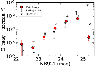
In Figure 9, we compare our average number counts with previous results where the selection criteria are similar to ours (Ouchi et al. 2008; Ouchi et al. 2010; Nakajima et al. 2012; Nakajima et al. 2013; Konno et al. 2016; Shibuya et al. 2018a; Hao et al. 2018; Itoh et al. 2018; Zhang et al. 2020; see also Table 7). We confirm that, in the magnitude ranges that have been probed in previous studies, our results are in good agreement with the previous results. On the other hand, comparisons of faint end results are not simple, because not only NBs but also BBs are involved, whose limiting magnitudes are not completely uniform between and within the survey fields. Because the $5\sigma$ limiting magnitudes of our $NB387$ data for most of our survey fields are $\simeq 24.3$–$24.7$ mag, the incompleteness effects in our number counts of $z=2.2$ LAEs are non-negligible at faint magnitudes of $NB387\gtrsim 24$ mag, compared to the previous results of Nakajima et al. (2012) and Hao et al. (2018), whose $5\sigma$ limiting magnitudes are $\sim 26$ mag. In contrast, although the $5\sigma$ limiting magnitudes of our $NB527$ data are deeper than those of the previous work at similar redshifts, the incompleteness effect in our number counts is significant at around $NB527\simeq 25$ mag, which is comparable to those of the previous results. This is probably because our BB data are relatively shallow. Similar discussion can be made for the results at higher redshifts.

Most of our survey fields have already been observed in our previous work (Shibuya et al. 2018a). We compare our LAE catalogs with those constructed in our previous work at $z=5.7$ and $z=6.6$ and calculate the object-matching rates as a function of NB magnitudes. We find that the object-matching rates are $\simeq 80$–$100$% at bright NB magnitudes of $\lesssim 24$ mag for the UD fields where the effect of photometric uncertainties is not relatively significant. The high object-matching rates indicate that we adequately select LAE candidates in our machine learning selection processes. Note that the object-matching rates decrease to $\simeq 60$–$70$% at the fainter magnitudes of $\simeq 24.5$–$25$ mag, mainly due to the increase of the effect of photometric uncertainties. We confirm that these object-matching rates are comparable to those obtained in Shibuya et al. (2018a).

We also compare our LAE catalogs with the results of our previous spectroscopic observations for high-$z$ galaxies in our survey fields including the ones with Magellan/IMACS (PI: M. Ouchi; M. Ouchi in prep.; Ono et al. 2018; Harikane et al. 2019), as well as the publicly available spectroscopic catalogs shown in previous studies (Saito et al. 2008; Ouchi et al. 2008; Willott et al. 2010; Ouchi et al. 2010; Masters et al. 2012; Mallery et al. 2012; Willott et al. 2013; McGreer et al. 2013; Le Fèvre et al. 2013; Shibuya et al. 2014; Kriek et al. 2015; Sobral et al. 2015; Wang et al. 2016; Hu et al. 2016; Toshikawa et al. 2016; Momcheva et al. 2016; Bañados et al. 2016; Tasca et al. 2017; Yang et al. 2017; Masters et al. 2017; Hu et al. 2017; Ikeda et al. 2017; Jiang et al. 2017; Suzuki et al. 2017; Shibuya et al. 2018b; Sobral et al. 2018; Lee et al. 2018; Pentericci et al. 2018; Jiang et al. 2018; Masters et al. 2019; Harikane et al. 2019; Calvi et al. 2019; Zhang et al. 2020; Lyke et al. 2020; Onodera et al. 2020). We adopt their classifications between galaxies and AGNs in their catalogs if available. For the catalogs of the VIMOS VLT Deep Survey (VVDS: Le Fèvre et al. 2013) and the VIMOS Ultra Deep Survey (VUDS: Tasca et al. 2017), we take into account sources whose redshifts are $>70$%–$75$% correct, i.e., sources with redshift reliability flags of 2, 3, 4, 9, 12, 13, 14, and 19.

We find that 177 LAEs in our samples have been spectroscopically confirmed by our observations and in the previous studies. Among them, 155 sources are found to be Ly$\alpha$-emitting galaxies, and the other 22 sources are Ly$\alpha$-emitting AGNs. The catalog of these spectroscopically confirmed LAEs is presented in Table A1. We confirm that their spectroscopic redshifts are consistent with those expected from the redshift coverages of the NBs used in this study. Their redshift distributions around the redshift ranges probed with the NBs are shown in Figure 10.

Figure 10.— Redshift distribution of spectroscopically confirmed LAEs in our samples (gray histograms). The colored curves are the best-fit results with the transmission curves of the NB filters shown in Figure 1. The blue, yellow, orange, and magenta curves correspond to the results with the $NB387$, $NB718$, $NB816$, and $NB921$ filter transmission curves, respectively. We do not perform the fitting for $z=3.3$ and $z=7.0$ because of the limited number of the data points.

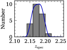
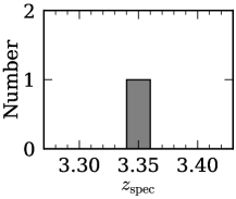
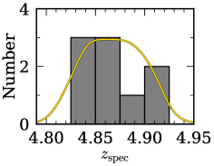
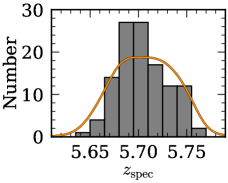
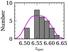
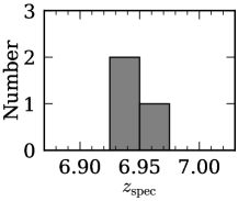
To characterize these redshift distributions, we fit the transmission curves of the NBs to them. Specifically, we derive the best-fit NB transmission curves by a $\chi^{2}$ minimization fit with a normalization constant and a redshift shift as free parameters, i.e., $N(z)=\alpha T(z+\beta)$, where $N(z)$ is the redshift distribution, $T(z)$ is the NB transmission curve, $\alpha$ is the normalization constant, and $\beta$ is the shift along the $x$-axis. The observed wavelengths of the NB transmission curves are converted to the Ly$\alpha$ redshifts, $z_{\rm Ly\alpha}$, by $z_{\rm Ly\alpha}=\lambda_{\rm obs}/\lambda_{{\rm Ly}\alpha}-1$, where $\lambda_{\rm obs}$ is the observed wavelength and $\lambda_{{\rm Ly}\alpha}=1215.67$Å is the Ly$\alpha$ wavelength. The best-fit results are shown in Figure 10, and the best-fit parameters are presented in Table 8. We do not perform the fitting for $z=3.3$ and $z=7.0$, because of the limited number of the data points. We find that the solid curves fit the histograms well. We also find that, the best-fit $\beta$ values for $NB718$, $NB816$, and $NB921$ are negative. This is probably because, for high redshift LAEs, although a high sensitivity for Ly$\alpha$ emission is necessary, a high sensitivity for continuum emission also makes it easier for the NBs to detect LAEs. Another possible reason is that the majority of the spectroscopic redshifts used for the compilation are based on the catalogs whose sources are found with instruments other than HSC.

In addition to the 177 spectroscopically confirmed LAEs, we notice that 4 sources in our sample have also been spectroscopically confirmed as lower-$z$ sources in the previous studies. In fact, these 4 source are AGNs at slightly lower redshift where strong Civ emission is probed with our NBs. The catalog of these sources is presented in Table A2. Although it is difficult to make a fair comparison based on the available catalogs, the small number of the spectroscopic identifications at low redshifts may suggest that the contamination rate of low-$z$ interlopers is low. However, it should be noted that, because our selections do not use BB data whose wavelengths are bluer than the Lyman limit for our $z=2.2$ and $z=3.3$ LAE samples, it is not surprising that these two samples are relatively contaminated by lower-$z$ interlopers such as strong [Oii] and [Oiii] emitters. Quantitative discussion for such possibilities is waiting to be examined with further spectroscopic observations.

5. Summary

We have constructed a catalog of $9$,$318$ LAE candidates at $z=2.2$, $3.3$, $4.9$, $5.7$, $6.6$, and $7.0$ with the aid of the machine learning technique based on the multiwavelength data over the $1.6$–$25.0$ deg² sky taken with the six narrowband filters of $NB387$, $NB527$, $NB718$, $NB816$, $NB921$, and $NB973$, and the five broadband filters of $g$, $r$, $i$, $z$, and $y$ in the HSC SSP and CHORUS. We have first photometrically selected LAE candidates based on the NB-excess features of their SEDs. We have then created the CNN, which is recently frequently adopted for image classification problems, to distinguish between real LAEs and contaminants. We have found that the completeness and contamination rate of the trained CNN are $94$% and $1$%, respectively. By taking advantage of the trained CNN, we have efficiently removed contaminants such as satellite trails and low-$z$ interlopers from the photometrically selected LAE candidates. Specifically, for all the photometrically selected LAE candidates, the amount of human effort to conduct visual inspection is estimated to be about 11 person-months, but we have significantly reduced it thanks to the CNN application. We have confirmed that our machine learning selected LAE samples are reliable on the basis of $177$ LAEs that have already been spectroscopically identified by our SILVERRUSH programs and previous studies. In addition, we have found that the object-matching rates between our LAE catalogs and our previous results are $\simeq 80$–$100$% at bright NB magnitudes of $\lesssim 24$ mag, which also supports the validity of our selection method. We have also confirmed that the surface number densities of our LAE candidates are consistent with previous results. Our LAE catalogs will become available online.

Appendix A A. Catalog of Spectroscopically Confirmed LAEs in Our Samples

In this paper, we present a catalog of spectroscopically confirmed galaxies and AGNs in our LAE samples in Table A1. In addition, we also present a catalog of spectroscopically confirmed AGNs that are selected with our NBs because of their strong Civ emission in Table A2. Our new SILVERRUSH LAE catalogs based on new HSC SSP and CHORUS data will be made public on our project webpage as described in Section 1.

Table A1Spectroscopically confirmed galaxies and AGNs in our LAE samples

ID	R.A.	Decl.	$z_{\rm spec}$	$g_{\rm ap}$	$r_{\rm ap}$	$i_{\rm ap}$	$z_{\rm ap}$	$y_{\rm ap}$	$NB_{\rm tot}$	Sample	Field	Flag	Reference
(1)	(2)	(3)	(4)	(5)	(6)	(7)	(8)	(9)	(10)	(11)	(12)	(13)	(14)
HSC J021525–045918	02:15:25.24	$-$04:59:18.12	$5.671$	$99.0$	$32.7$	$26.6$	$26.0$	$25.5$	$24.2$	NB816	UDSXDS	1	This study
HSC J021526–045229	02:15:26.23	$-$04:52:29.83	$5.655$	$99.0$	$29.6$	$26.2$	$25.3$	$24.9$	$24.6$	NB816	UDSXDS	1	This study
HSC J021533–050137	02:15:33.24	$-$05:01:37.38	$5.671$	$29.2$	$28.1$	$26.3$	$25.6$	$25.4$	$24.4$	NB816	UDSXDS	1	This study
HSC J021551–045325	02:15:51.35	$-$04:53:25.47	$5.710$	$31.5$	$28.8$	$99.0$	$27.3$	$28.0$	$25.2$	NB816	UDSXDS	1	This study
HSC J021555–045318	02:15:55.65	$-$04:53:18.83	$5.738$	$28.9$	$28.6$	$28.0$	$28.0$	$99.0$	$25.4$	NB816	UDSXDS	1	This study
HSC J021558–045301	02:15:58.50	$-$04:53:01.82	$5.718$	$99.0$	$99.0$	$27.4$	$28.3$	$99.0$	$24.6$	NB816	UDSXDS	1	This study
HSC J021611–045633	02:16:11.37	$-$04:56:33.13	$6.549$	$30.0$	$99.0$	$99.0$	$27.2$	$27.0$	$25.0$	NB921	UDSXDS	1	This study
HSC J021617–045419	02:16:17.15	$-$04:54:19.37	$5.707$	$99.0$	$99.0$	$29.2$	$29.4$	$29.2$	$25.5$	NB816	UDSXDS	1	This study
HSC J021624–045516	02:16:24.70	$-$04:55:16.61	$5.706$	$99.0$	$99.0$	$26.4$	$25.9$	$26.9$	$23.5$	NB816	UDSXDS	1	This study
HSC J021625–045237	02:16:25.64	$-$04:52:37.24	$5.730$	$99.0$	$31.9$	$28.9$	$30.0$	$99.0$	$25.0$	NB816	UDSXDS	1	This study
HSC J021628–050103	02:16:28.06	$-$05:01:03.96	$5.692$	$30.9$	$99.0$	$28.3$	$27.3$	$27.3$	$25.0$	NB816	UDSXDS	1	This study
HSC J021636–044723	02:16:36.44	$-$04:47:23.69	$5.718$	$99.0$	$99.0$	$27.0$	$27.0$	$27.5$	$24.9$	NB816	UDSXDS	1	This study
HSC J021654–045556	02:16:54.54	$-$04:55:56.99	$6.617$	$99.0$	$99.0$	$99.0$	$27.0$	$26.9$	$25.0$	NB921	UDSXDS	1	O10
HSC J021654–052155	02:16:54.61	$-$05:21:55.74	$5.712$	$30.2$	$99.0$	$27.1$	$26.9$	$26.8$	$24.3$	NB816	UDSXDS	1	H19
HSC J021657–052117	02:16:57.89	$-$05:21:17.06	$5.667$	$99.0$	$99.0$	$26.8$	$26.3$	$29.1$	$25.2$	NB816	UDSXDS	1	H19
HSC J021702–050604	02:17:02.57	$-$05:06:04.71	$6.545$	$99.0$	$27.9$	$28.9$	$26.4$	$28.3$	$24.6$	NB921	UDSXDS	1	O10
HSC J021703–045619	02:17:03.47	$-$04:56:19.14	$6.589$	$99.0$	$99.0$	$99.0$	$27.0$	$26.3$	$24.7$	NB921	UDSXDS	1	O10
HSC J021704–052714	02:17:04.30	$-$05:27:14.43	$5.686$	$99.0$	$28.2$	$26.4$	$26.2$	$26.5$	$24.2$	NB816	UDSXDS	1	H19
HSC J021707–053426	02:17:07.86	$-$05:34:26.78	$5.678$	$99.0$	$99.0$	$27.1$	$26.5$	$99.0$	$24.2$	NB816	UDSXDS	1	H19
HSC J021709–050329	02:17:09.78	$-$05:03:29.34	$5.709$	$29.3$	$29.2$	$27.4$	$27.0$	$99.0$	$24.6$	NB816	UDSXDS	1	This study
HSC J021709–052646	02:17:09.97	$-$05:26:46.76	$5.689$	$99.0$	$99.0$	$28.5$	$27.1$	$99.0$	$25.2$	NB816	UDSXDS	1	H19
HSC J021719–043150	02:17:19.13	$-$04:31:50.71	$5.735$	$99.0$	$99.0$	$27.9$	$27.5$	$28.7$	$24.3$	NB816	UDSXDS	1	This study
HSC J021724–053309	02:17:24.04	$-$05:33:09.78	$5.707$	$31.1$	$99.0$	$25.9$	$25.4$	$26.5$	$23.3$	NB816	UDSXDS	1	S18
HSC J021725–050737	02:17:25.90	$-$05:07:37.65	$5.701$	$99.0$	$99.0$	$27.9$	$27.2$	$26.6$	$24.7$	NB816	UDSXDS	1	This study
HSC J021726–045126	02:17:26.74	$-$04:51:26.79	$5.709$	$99.0$	$99.0$	$27.5$	$99.0$	$99.0$	$24.9$	NB816	UDSXDS	1	This study
HSC J021729–053028	02:17:29.19	$-$05:30:28.61	$5.746$	$99.0$	$28.9$	$28.0$	$28.5$	$99.0$	$25.0$	NB816	UDSXDS	1	H19
HSC J021734–053452	02:17:34.16	$-$05:34:52.80	$5.708$	$99.0$	$99.0$	$99.0$	$27.9$	$99.0$	$25.2$	NB816	UDSXDS	1	H19
HSC J021734–044559	02:17:34.58	$-$04:45:59.04	$5.701$	$28.7$	$29.4$	$26.6$	$25.9$	$25.8$	$24.3$	NB816	UDSXDS	1	This study
HSC J021736–052701	02:17:36.39	$-$05:27:01.90	$5.672$	$28.2$	$99.0$	$26.8$	$26.4$	$99.0$	$24.1$	NB816	UDSXDS	1	H19
HSC J021736–053027	02:17:36.68	$-$05:30:27.60	$5.686$	$99.0$	$99.0$	$27.9$	$26.8$	$99.0$	$25.4$	NB816	UDSXDS	1	H19
HSC J021737–043943	02:17:37.97	$-$04:39:43.12	$5.755$	$29.5$	$99.0$	$26.9$	$26.2$	$25.8$	$24.5$	NB816	UDSXDS	1	This study
HSC J021739–043837	02:17:39.26	$-$04:38:37.38	$5.721$	$99.0$	$99.0$	$28.6$	$26.8$	$99.0$	$24.6$	NB816	UDSXDS	1	This study
HSC J021742–052810	02:17:42.18	$-$05:28:10.64	$5.679$	$99.0$	$28.9$	$27.2$	$26.3$	$26.0$	$25.1$	NB816	UDSXDS	1	H19
HSC J021743–052807	02:17:43.34	$-$05:28:07.05	$5.685$	$28.1$	$27.4$	$26.2$	$26.0$	$26.1$	$24.0$	NB816	UDSXDS	1	O08
HSC J021745–052842	02:17:45.03	$-$05:28:42.58	$5.751$	$99.0$	$28.9$	$26.7$	$25.6$	$25.9$	$24.4$	NB816	UDSXDS	1	O08
HSC J021745–052936	02:17:45.25	$-$05:29:36.17	$5.688$	$99.0$	$99.0$	$26.9$	$26.4$	$27.4$	$24.2$	NB816	UDSXDS	1	O08
HSC J021745–044129	02:17:45.75	$-$04:41:29.34	$5.674$	$28.1$	$99.0$	$26.9$	$29.4$	$27.9$	$24.9$	NB816	UDSXDS	1	This study
HSC J021748–053127	02:17:48.47	$-$05:31:27.17	$5.690$	$99.0$	$29.3$	$27.4$	$26.5$	$26.3$	$24.6$	NB816	UDSXDS	1	O08
HSC J021749–052854	02:17:49.12	$-$05:28:54.24	$5.696$	$28.6$	$28.6$	$26.4$	$25.6$	$25.8$	$24.0$	NB816	UDSXDS	1	O08
HSC J021749–052708	02:17:49.99	$-$05:27:08.36	$5.693$	$99.0$	$99.0$	$27.8$	$26.7$	$25.9$	$24.2$	NB816	UDSXDS	1	O08
HSC J021750–050203	02:17:50.87	$-$05:02:03.33	$5.708$	$28.8$	$27.9$	$27.1$	$26.7$	$27.5$	$24.7$	NB816	UDSXDS	1	This study
HSC J021751–053003	02:17:51.15	$-$05:30:03.78	$5.712$	$99.0$	$29.6$	$27.9$	$26.4$	$25.9$	$25.1$	NB816	UDSXDS	1	O08
HSC J021752–053511	02:17:52.64	$-$05:35:11.79	$5.756$	$28.2$	$27.5$	$25.3$	$24.7$	$24.6$	$23.1$	NB816	UDSXDS	1	S18
HSC J021755–043251	02:17:55.41	$-$04:32:51.63	$5.690$	$99.0$	$30.2$	$27.1$	$26.9$	$26.7$	$24.6$	NB816	UDSXDS	1	This study
HSC J021757–050844	02:17:57.58	$-$05:08:44.70	$6.595$	$99.0$	$99.0$	$99.0$	$25.6$	$25.6$	$23.3$	NB921	UDSXDS	1	O10
HSC J021757–053309	02:17:57.67	$-$05:33:09.50	$5.749$	$99.0$	$29.0$	$27.1$	$26.6$	$25.6$	$24.3$	NB816	UDSXDS	1	H19
HSC J021758–043030	02:17:58.92	$-$04:30:30.46	$5.689$	$99.0$	$99.0$	$26.7$	$26.1$	$25.8$	$24.2$	NB816	UDSXDS	1	This study
HSC J021800–053518	02:18:00.73	$-$05:35:18.99	$5.673$	$99.0$	$30.9$	$26.4$	$25.3$	$25.0$	$24.8$	NB816	UDSXDS	1	H19
HSC J021802–052011	02:18:02.19	$-$05:20:11.58	$5.718$	$99.0$	$29.8$	$28.5$	$28.6$	$99.0$	$25.3$	NB816	UDSXDS	1	H19
HSC J021803–052643	02:18:03.89	$-$05:26:43.51	$5.747$	$99.0$	$28.5$	$27.5$	$27.1$	$29.3$	$24.7$	NB816	UDSXDS	1	H19
HSC J021804–052147	02:18:04.18	$-$05:21:47.31	$5.734$	$99.0$	$29.1$	$26.9$	$25.6$	$26.3$	$24.4$	NB816	UDSXDS	1	H19
HSC J021805–052704	02:18:05.19	$-$05:27:04.20	$5.746$	$99.0$	$99.0$	$26.9$	$27.3$	$26.6$	$24.8$	NB816	UDSXDS	1	H19
HSC J021805–052027	02:18:05.30	$-$05:20:27.04	$5.742$	$99.0$	$99.0$	$28.6$	$26.8$	$99.0$	$25.0$	NB816	UDSXDS	1	H19
HSC J021806–042847	02:18:06.16	$-$04:28:47.66	$5.726$	$31.6$	$99.0$	$28.1$	$27.9$	$26.9$	$25.3$	NB816	UDSXDS	1	This study
HSC J021806–044510	02:18:06.23	$-$04:45:10.90	$6.576$	$28.1$	$28.8$	$27.8$	$26.7$	$25.4$	$24.4$	NB921	UDSXDS	1	This study
HSC J021810–053707	02:18:10.68	$-$05:37:07.93	$5.747$	$99.0$	$28.1$	$26.8$	$27.1$	$26.4$	$24.3$	NB816	UDSXDS	1	This study
HSC J021814–053249	02:18:14.41	$-$05:32:49.15	$5.673$	$29.3$	$30.8$	$26.9$	$25.9$	$25.9$	$24.9$	NB816	UDSXDS	1	O08
HSC J021819–050355	02:18:19.58	$-$05:03:55.46	$5.743$	$99.0$	$99.0$	$27.0$	$26.2$	$25.8$	$24.7$	NB816	UDSXDS	1	This study
HSC J021820–051109	02:18:20.70	$-$05:11:09.95	$6.575$	$99.0$	$28.8$	$99.0$	$27.4$	$26.8$	$24.7$	NB921	UDSXDS	1	O10
HSC J021822–042926	02:18:22.92	$-$04:29:26.05	$5.697$	$99.0$	$99.0$	$29.7$	$99.0$	$99.0$	$25.4$	NB816	UDSXDS	1	This study
HSC J021823–043524	02:18:23.54	$-$04:35:24.03	$6.519$	$99.0$	$99.0$	$99.0$	$26.5$	$25.5$	$24.6$	NB921	UDSXDS	1	O10
HSC J021825–050700	02:18:25.43	$-$05:07:00.63	$5.683$	$29.2$	$99.0$	$99.0$	$29.3$	$99.0$	$25.5$	NB816	UDSXDS	1	This study
HSC J021827–050726	02:18:27.01	$-$05:07:26.98	$6.554$	$29.0$	$99.0$	$28.0$	$27.7$	$99.0$	$25.0$	NB921	UDSXDS	1	O10
HSC J021827–043508	02:18:27.02	$-$04:35:08.06	$6.511$	$29.4$	$29.5$	$27.7$	$25.9$	$25.5$	$24.5$	NB921	UDSXDS	1	O10
HSC J021827–044737	02:18:27.45	$-$04:47:37.13	$5.703$	$99.0$	$99.0$	$26.6$	$26.5$	$26.1$	$23.7$	NB816	UDSXDS	1	This study
HSC J021828–051423	02:18:28.89	$-$05:14:23.09	$5.737$	$28.5$	$99.0$	$26.8$	$26.7$	$26.3$	$23.9$	NB816	UDSXDS	1	H19
HSC J021830–051457	02:18:30.53	$-$05:14:57.79	$5.688$	$99.0$	$28.5$	$26.3$	$26.5$	$26.7$	$23.9$	NB816	UDSXDS	1	H19
HSC J021830–052950	02:18:30.76	$-$05:29:50.39	$5.706$	$99.0$	$28.5$	$26.6$	$26.7$	$25.5$	$24.1$	NB816	UDSXDS	1	This study
HSC J021835–042321	02:18:35.95	$-$04:23:21.69	$5.755$	$99.0$	$99.0$	$25.7$	$25.4$	$25.8$	$23.2$	NB816	UDSXDS	1	S18
HSC J021836–053528	02:18:36.38	$-$05:35:28.14	$5.698$	$28.6$	$99.0$	$26.2$	$26.0$	$25.1$	$23.6$	NB816	UDSXDS	1	This study
HSC J021842–043011	02:18:42.59	$-$04:30:11.40	$6.548$	$30.4$	$29.8$	$99.0$	$26.7$	$26.8$	$24.6$	NB921	UDSXDS	1	This study
HSC J021843–050915	02:18:43.64	$-$05:09:15.71	$6.512$	$28.7$	$28.5$	$28.1$	$26.0$	$25.8$	$23.8$	NB921	UDSXDS	1	S18
HSC J021844–043636	02:18:44.66	$-$04:36:36.27	$6.621$	$30.0$	$99.0$	$99.0$	$26.2$	$27.3$	$24.4$	NB921	UDSXDS	1	O10
HSC J021845–052915	02:18:45.03	$-$05:29:15.91	$5.660$	$99.0$	$28.9$	$26.7$	$25.9$	$26.0$	$24.9$	NB816	UDSXDS	1	This study
HSC J021846–043722	02:18:46.66	$-$04:37:22.48	$5.735$	$99.0$	$99.0$	$27.6$	$28.1$	$26.8$	$24.7$	NB816	UDSXDS	1	This study
HSC J021848–051715	02:18:48.23	$-$05:17:15.65	$5.741$	$27.9$	$99.0$	$26.8$	$26.1$	$25.7$	$24.5$	NB816	UDSXDS	1	This study
HSC J021849–052235	02:18:49.01	$-$05:22:35.37	$5.718$	$99.0$	$99.0$	$26.5$	$26.4$	$26.4$	$24.4$	NB816	UDSXDS	1	This study
HSC J021850–053007	02:18:50.99	$-$05:30:07.79	$5.705$	$99.0$	$99.0$	$27.1$	$26.3$	$25.4$	$24.2$	NB816	UDSXDS	1	This study
HSC J021857–045648	02:18:57.32	$-$04:56:48.95	$5.681$	$99.0$	$99.0$	$28.0$	$28.0$	$99.0$	$25.3$	NB816	UDSXDS	1	This study
HSC J021859–052916	02:18:59.93	$-$05:29:16.77	$5.674$	$99.0$	$28.1$	$25.7$	$24.8$	$24.6$	$24.1$	NB816	UDSXDS	1	This study
HSC J021901–045859	02:19:01.43	$-$04:58:59.06	$6.553$	$30.8$	$31.4$	$29.6$	$26.8$	$26.4$	$24.6$	NB921	UDSXDS	1	This study
HSC J021911–045707	02:19:11.04	$-$04:57:07.60	$5.704$	$99.0$	$99.0$	$27.8$	$29.0$	$99.0$	$25.2$	NB816	UDSXDS	1	This study
HSC J021933–050820	02:19:33.13	$-$05:08:20.83	$6.590$	$99.0$	$99.0$	$99.0$	$27.2$	$26.8$	$24.9$	NB921	UDSXDS	1	This study
HSC J021943–044914	02:19:43.92	$-$04:49:14.43	$5.684$	$99.0$	$99.0$	$27.9$	$27.0$	$99.0$	$25.5$	NB816	UDSXDS	1	This study
HSC J022001–045839	02:20:01.06	$-$04:58:39.73	$5.682$	$99.0$	$99.0$	$27.5$	$28.6$	$26.5$	$25.4$	NB816	UDSXDS	1	This study
HSC J022001–051637	02:20:01.11	$-$05:16:37.43	$5.711$	$99.0$	$29.2$	$26.2$	$25.8$	$25.5$	$23.4$	NB816	UDSXDS	1	S18
HSC J022003–045416	02:20:03.20	$-$04:54:16.58	$5.697$	$99.0$	$99.0$	$26.4$	$25.3$	$25.1$	$23.9$	NB816	UDSXDS	1	This study
HSC J022012–044950	02:20:12.14	$-$04:49:50.97	$5.681$	$30.7$	$28.2$	$26.9$	$27.5$	$99.0$	$24.8$	NB816	UDSXDS	1	O08
HSC J022013–045109	02:20:13.33	$-$04:51:09.49	$5.744$	$27.9$	$27.5$	$26.3$	$25.9$	$25.4$	$24.0$	NB816	UDSXDS	1	O08
HSC J022026–050542	02:20:26.83	$-$05:05:42.43	$6.566$	$99.0$	$99.0$	$99.0$	$27.0$	$99.0$	$25.1$	NB921	UDSXDS	1	This study
HSC J022026–045217	02:20:26.88	$-$04:52:17.86	$5.720$	$99.0$	$28.8$	$26.5$	$26.1$	$25.5$	$24.8$	NB816	UDSXDS	1	This study
HSC J095919+020322	09:59:19.74	02:03:22.02	$5.704$	$99.0$	$99.0$	$28.0$	$28.3$	$27.4$	$24.5$	NB816	UDCOSMOS	1	M12
HSC J095922+021029	09:59:22.27	02:10:29.28	$5.716$	$29.2$	$29.0$	$27.2$	$28.6$	$27.5$	$25.2$	NB816	UDCOSMOS	1	This study
HSC J095929+022950	09:59:29.35	02:29:50.17	$4.840$	$99.0$	$28.0$	$25.8$	$26.0$	$25.9$	$24.7$	NB718	UDCOSMOS	1	M12
HSC J095930+021642	09:59:30.08	02:16:42.79	$5.680$	$28.0$	$27.7$	$27.0$	$26.7$	$26.8$	$25.1$	NB816	UDCOSMOS	1	M12
HSC J095933+024955	09:59:33.43	02:49:55.93	$5.724$	$29.7$	$27.8$	$26.6$	$27.0$	$28.4$	$24.1$	NB816	UDCOSMOS	1	M12
HSC J095944+020050	09:59:44.06	02:00:50.62	$5.688$	$31.6$	$30.0$	$26.9$	$26.2$	$26.9$	$24.4$	NB816	UDCOSMOS	1	M12
HSC J095945+022807	09:59:45.97	02:28:07.84	$2.174$	$24.9$	$24.9$	$24.8$	$24.7$	$24.9$	$24.1$	NB387	DCOSMOS	1	S14
HSC J095946+014353	09:59:46.13	01:43:53.09	$5.717$	$99.0$	$99.0$	$27.4$	$27.3$	$27.0$	$25.1$	NB816	UDCOSMOS	1	M12
HSC J095952+015005	09:59:52.02	01:50:05.75	$5.744$	$99.0$	$29.5$	$26.4$	$25.5$	$25.4$	$24.1$	NB816	UDCOSMOS	1	M12
HSC J095952+013723	09:59:52.13	01:37:23.18	$5.724$	$99.0$	$30.6$	$26.5$	$26.0$	$26.0$	$24.1$	NB816	UDCOSMOS	1	M12
HSC J095953+020705	09:59:53.25	02:07:05.35	$5.692$	$29.2$	$28.4$	$25.8$	$24.6$	$24.5$	$23.6$	NB816	UDCOSMOS	1	M12
HSC J095954+022629	09:59:54.39	02:26:29.99	$2.194$	$25.0$	$24.6$	$24.3$	$24.0$	$23.7$	$23.1$	NB387	UDCOSMOS	1	S14
HSC J095954+021516	09:59:54.52	02:15:16.56	$5.688$	$99.0$	$99.0$	$27.1$	$26.9$	$27.6$	$24.8$	NB816	UDCOSMOS	1	M12
HSC J095954+021039	09:59:54.77	02:10:39.26	$5.662$	$33.7$	$28.6$	$26.7$	$26.5$	$26.4$	$24.9$	NB816	UDCOSMOS	1	M12
HSC J095955+014720	09:59:55.00	01:47:20.65	$5.715$	$99.0$	$99.0$	$26.7$	$26.0$	$25.9$	$24.1$	NB816	UDCOSMOS	1	M12
HSC J100004+020845	10:00:04.17	02:08:45.65	$4.840$	$99.0$	$26.7$	$25.0$	$25.2$	$25.2$	$24.0$	NB718	UDCOSMOS	1	M12
HSC J100005+020717	10:00:05.05	02:07:17.00	$5.704$	$99.0$	$99.0$	$27.9$	$27.2$	$27.9$	$24.3$	NB816	UDCOSMOS	1	M12
HSC J100019+020103	10:00:19.98	02:01:03.21	$5.645$	$99.0$	$99.0$	$27.2$	$26.9$	$26.6$	$25.6$	NB816	UDCOSMOS	1	M12
HSC J100029+024115	10:00:29.12	02:41:15.66	$5.735$	$99.0$	$27.3$	$26.5$	$26.4$	$26.8$	$23.4$	NB816	UDCOSMOS	1	M12
HSC J100029+015000	10:00:29.58	01:50:00.69	$5.707$	$30.6$	$29.4$	$27.3$	$26.5$	$26.9$	$24.9$	NB816	UDCOSMOS	1	M12
HSC J100030+021714	10:00:30.40	02:17:14.78	$5.695$	$99.0$	$99.0$	$27.6$	$26.8$	$26.9$	$24.4$	NB816	UDCOSMOS	1	M12
HSC J100030+013621	10:00:30.43	01:36:21.70	$4.844$	$29.4$	$27.7$	$25.8$	$26.0$	$26.1$	$24.8$	NB718	UDCOSMOS	1	M12
HSC J100034+013616	10:00:34.61	01:36:16.15	$4.902$	$28.8$	$27.1$	$25.5$	$25.4$	$25.2$	$24.4$	NB718	UDCOSMOS	1	M12
HSC J100040+021903	10:00:40.23	02:19:03.66	$5.719$	$99.0$	$30.5$	$27.3$	$26.8$	$27.4$	$24.5$	NB816	UDCOSMOS	1	M12
HSC J100041+022637	10:00:41.08	02:26:37.33	$4.867$	$99.0$	$27.4$	$25.7$	$25.8$	$26.0$	$24.0$	NB718	UDCOSMOS	1	M12
HSC J100042+022019	10:00:42.19	02:20:19.55	$5.661$	$28.1$	$27.9$	$26.7$	$26.2$	$25.9$	$24.8$	NB816	UDCOSMOS	1	This study
HSC J100055+021309	10:00:55.43	02:13:09.13	$4.872$	$99.0$	$29.4$	$26.2$	$26.4$	$28.4$	$23.9$	NB718	UDCOSMOS	1	M12
HSC J100055+013630	10:00:55.52	01:36:30.84	$5.670$	$29.8$	$28.6$	$26.8$	$26.4$	$26.4$	$25.2$	NB816	UDCOSMOS	1	M12
HSC J100058+014815	10:00:58.00	01:48:15.08	$6.604$	$99.0$	$30.9$	$29.8$	$25.5$	$24.8$	$23.1$	NB921	UDCOSMOS	1	S15
HSC J100058+013642	10:00:58.41	01:36:42.77	$5.688$	$32.0$	$28.1$	$27.0$	$27.2$	$26.1$	$24.7$	NB816	UDCOSMOS	1	M12
HSC J100102+015144	10:01:02.96	01:51:44.74	$5.666$	$31.9$	$28.1$	$26.6$	$26.2$	$26.2$	$24.7$	NB816	UDCOSMOS	1	M12
HSC J100107+015222	10:01:07.35	01:52:22.69	$5.668$	$99.0$	$99.0$	$27.4$	$27.0$	$99.0$	$25.5$	NB816	UDCOSMOS	1	M12
HSC J100109+021513	10:01:09.72	02:15:13.47	$5.712$	$28.1$	$29.1$	$25.9$	$25.9$	$25.8$	$23.1$	NB816	UDCOSMOS	1	M12
HSC J100110+022829	10:01:10.06	02:28:29.03	$5.681$	$99.0$	$28.0$	$26.1$	$25.0$	$25.0$	$24.2$	NB816	UDCOSMOS	1	M12
HSC J100122+022249	10:01:22.45	02:22:49.83	$4.871$	$29.8$	$29.0$	$26.5$	$26.6$	$26.5$	$24.5$	NB718	UDCOSMOS	1	M12
HSC J100123+015600	10:01:23.84	01:56:00.29	$5.726$	$99.0$	$99.0$	$26.5$	$25.9$	$25.9$	$23.6$	NB816	UDCOSMOS	1	M12
HSC J100124+023145	10:01:24.79	02:31:45.48	$6.541$	$29.9$	$28.5$	$27.5$	$25.6$	$25.6$	$23.5$	NB921	UDCOSMOS	1	S15
HSC J100126+014430	10:01:26.89	01:44:30.15	$5.686$	$99.0$	$99.0$	$26.7$	$26.3$	$26.0$	$24.6$	NB816	UDCOSMOS	1	M12
HSC J100127+023005	10:01:27.76	02:30:05.89	$5.696$	$29.4$	$28.4$	$26.7$	$26.0$	$26.1$	$24.2$	NB816	UDCOSMOS	1	M12
HSC J100129+014929	10:01:29.08	01:49:29.79	$5.707$	$99.0$	$29.7$	$26.2$	$25.6$	$25.5$	$23.1$	NB816	UDCOSMOS	1	M12
HSC J100131+023105	10:01:31.07	02:31:05.81	$5.690$	$30.5$	$99.0$	$26.9$	$26.9$	$26.8$	$24.4$	NB816	UDCOSMOS	1	M12
HSC J100131+014320	10:01:31.12	01:43:20.31	$5.728$	$29.7$	$28.4$	$26.8$	$26.3$	$26.5$	$24.4$	NB816	UDCOSMOS	1	M12
HSC J100145+015712	10:01:45.12	01:57:12.23	$4.909$	$99.0$	$26.6$	$25.1$	$25.0$	$24.9$	$23.6$	NB718	UDCOSMOS	1	M12
HSC J100146+014827	10:01:46.64	01:48:27.07	$5.704$	$99.0$	$28.3$	$27.0$	$27.0$	$27.6$	$24.4$	NB816	UDCOSMOS	1	This study
HSC J100153+020459	10:01:53.45	02:04:59.79	$6.931$	$30.4$	$28.8$	$27.7$	$27.2$	$25.5$	$24.3$	NB973	UDCOSMOS	1	H17
HSC J100205+020646	10:02:05.96	02:06:46.15	$6.936$	$99.0$	$99.0$	$99.0$	$99.0$	$25.3$	$24.0$	NB973	UDCOSMOS	1	H17
HSC J100207+023217	10:02:07.81	02:32:17.18	$6.616$	$99.0$	$30.7$	$30.5$	$27.0$	$26.6$	$24.9$	NB921	UDCOSMOS	1	This study
HSC J100208+015445	10:02:08.80	01:54:45.04	$5.676$	$29.4$	$27.8$	$26.1$	$26.0$	$25.7$	$24.3$	NB816	UDCOSMOS	1	M12
HSC J100214+021242	10:02:14.21	02:12:42.92	$5.731$	$31.7$	$99.0$	$27.4$	$26.6$	$26.8$	$24.6$	NB816	UDCOSMOS	1	This study
HSC J100215+024033	10:02:15.51	02:40:33.39	$6.965$	$27.5$	$27.3$	$27.2$	$27.4$	$25.2$	$23.4$	NB973	UDCOSMOS	1	Z20
HSC J100235+021213	10:02:35.37	02:12:13.89	$6.593$	$27.0$	$26.8$	$26.4$	$25.1$	$25.2$	$23.1$	NB921	UDCOSMOS	1	H16
HSC J100301+020235	10:03:01.14	02:02:35.99	$5.682$	$99.0$	$28.8$	$26.1$	$25.0$	$25.0$	$24.1$	NB816	UDCOSMOS	1	M12
HSC J100301+015011	10:03:01.81	01:50:11.15	$5.695$	$28.3$	$27.0$	$25.5$	$25.1$	$24.6$	$23.5$	NB816	UDCOSMOS	1	M12
HSC J100305+015141	10:03:05.33	01:51:41.09	$5.694$	$30.6$	$29.0$	$27.2$	$26.5$	$26.0$	$24.7$	NB816	UDCOSMOS	1	M12
HSC J100306+014742	10:03:06.12	01:47:42.69	$5.680$	$99.0$	$99.0$	$26.9$	$26.9$	$27.0$	$24.7$	NB816	UDCOSMOS	1	M12
HSC J100334+024546	10:03:34.67	02:45:46.58	$6.586$	$28.3$	$28.1$	$99.0$	$25.6$	$25.3$	$23.8$	NB921	DCOSMOS	1	S18
HSC J160107+550720	16:01:07.45	55:07:20.58	$6.573$	$28.9$	$99.0$	$99.0$	$26.0$	$25.5$	$23.7$	NB921	DELAISN1	1	S18
HSC J160707+555347	16:07:07.45	55:53:47.82	$6.564$	$99.0$	$99.0$	$99.0$	$26.2$	$99.0$	$24.0$	NB921	DELAISN1	1	S18
HSC J160940+541409	16:09:40.24	54:14:09.06	$6.575$	$27.8$	$27.6$	$27.1$	$25.6$	$26.0$	$23.9$	NB921	DELAISN1	1	S18
HSC J162126+545719	16:21:26.50	54:57:19.09	$6.545$	$28.3$	$99.0$	$27.9$	$24.5$	$24.0$	$22.4$	NB921	DELAISN1	1	S18
HSC J232558–002557	23:25:58.44	$-$00:25:57.56	$5.703$	$99.0$	$28.1$	$25.6$	$25.2$	$25.5$	$23.3$	NB816	DDEEP23	1	S18
HSC J233125–005216	23:31:25.36	$-$00:52:16.49	$6.559$	$99.0$	$99.0$	$99.0$	$25.5$	$99.0$	$23.1$	NB921	DDEEP23	1	S18
HSC J233408–004403	23:34:08.80	$-$00:44:03.69	$5.707$	$28.1$	$99.0$	$25.5$	$25.9$	$26.6$	$22.7$	NB816	DDEEP23	1	S18
HSC J233454–003603	23:34:54.95	$-$00:36:03.97	$5.732$	$31.2$	$27.5$	$25.5$	$25.2$	$24.9$	$23.0$	NB816	DDEEP23	1	S18
HSC J022028–045802	02:20:28.96	$-$04:58:02.81	$2.157$	$20.6$	$20.7$	$20.4$	$20.1$	$20.2$	$19.1$	NB387	DSXDS	2	L20
HSC J022120–032353	02:21:20.93	$-$03:23:53.52	$2.183$	$22.9$	$22.6$	$22.6$	$22.3$	$99.0$	$21.2$	NB387	DSXDS	2	L20
HSC J022121–034338	02:21:21.16	$-$03:43:38.10	$2.176$	$23.2$	$23.2$	$23.1$	$22.7$	$22.7$	$21.8$	NB387	DSXDS	2	L20
HSC J022202–050351	02:22:02.59	$-$05:03:51.98	$2.161$	$21.8$	$21.7$	$21.6$	$21.3$	$21.6$	$20.4$	NB387	DSXDS	2	L20
HSC J022219–052231	02:22:19.95	$-$05:22:31.54	$2.204$	$20.4$	$20.1$	$20.2$	$19.9$	$20.1$	$19.3$	NB387	DSXDS	2	L20
HSC J022230–033545	02:22:30.42	$-$03:35:45.37	$2.172$	$22.1$	$22.2$	$22.0$	$21.5$	$21.8$	$19.9$	NB387	DSXDS	2	L20
HSC J022312–050625	02:23:12.46	$-$05:06:25.07	$2.190$	$20.1$	$20.1$	$20.1$	$19.8$	$19.9$	$19.1$	NB387	DSXDS	2	L20
HSC J022349–033930	02:23:49.43	$-$03:39:30.65	$2.141$	$21.1$	$20.8$	$20.8$	$20.5$	$20.8$	$19.9$	NB387	DSXDS	2	L20
HSC J022351–044730	02:23:51.07	$-$04:47:30.05	$2.167$	$20.7$	$20.6$	$20.7$	$20.3$	$20.4$	$19.5$	NB387	DSXDS	2	L20
HSC J095508+011205	09:55:08.45	01:12:05.71	$2.166$	$21.9$	$21.9$	$21.7$	$21.3$	$21.5$	$19.9$	NB387	DCOSMOS	2	L20
HSC J095539+011316	09:55:39.50	01:13:16.30	$2.142$	$21.6$	$21.6$	$21.6$	$21.1$	$21.4$	$20.3$	NB387	DCOSMOS	2	L20
HSC J095714+013145	09:57:14.02	01:31:45.51	$2.142$	$21.7$	$21.6$	$21.4$	$21.0$	$21.2$	$20.0$	NB387	DCOSMOS	2	L20
HSC J095822+010806	09:58:22.03	01:08:06.39	$2.171$	$20.8$	$20.7$	$20.7$	$20.3$	$20.4$	$19.4$	NB387	DCOSMOS	2	L20
HSC J095930+024124	09:59:30.21	02:41:24.95	$2.187$	$22.0$	$22.0$	$21.6$	$21.2$	$21.4$	$20.6$	NB387	DCOSMOS	2	L20
HSC J100057+023932	10:00:57.79	02:39:32.48	$3.360$	$23.6$	$22.9$	$22.9$	$22.8$	$22.8$	$22.0$	NB527	UDCOSMOS	2	Mas12
HSC J100145+020244	10:01:45.97	02:02:44.35	$4.888$	$30.5$	$25.8$	$24.1$	$24.1$	$24.2$	$22.6$	NB718	UDCOSMOS	2	Z20
HSC J232459–001451	23:24:59.71	$-$00:14:51.21	$2.172$	$21.4$	$21.2$	$21.2$	$20.8$	$21.0$	$19.6$	NB387	DDEEP23	2	L20
HSC J232506–012203	23:25:06.73	$-$01:22:03.29	$2.181$	$20.4$	$20.4$	$20.3$	$20.1$	$20.2$	$19.1$	NB387	DDEEP23	2	L20
HSC J232619–000152	23:26:19.35	$-$00:01:52.72	$2.173$	$22.1$	$22.1$	$21.6$	$21.5$	$21.7$	$20.8$	NB387	DDEEP23	2	L20
HSC J232855–004212	23:28:55.78	$-$00:42:12.22	$2.198$	$20.5$	$20.4$	$20.1$	$19.8$	$19.9$	$19.1$	NB387	DDEEP23	2	L20
HSC J233159–000856	23:31:59.69	$-$00:08:56.47	$2.184$	$20.8$	$20.6$	$20.6$	$20.3$	$20.4$	$19.6$	NB387	DDEEP23	2	L20
HSC J233217–011416	23:32:17.04	$-$01:14:16.90	$2.168$	$99.0$	$21.1$	$20.9$	$20.6$	$20.7$	$19.8$	NB387	DDEEP23	2	L20

Note. — (1) Object ID. (2) Right Ascension. (3) Declination. (4) Spectroscopic redshift. (5)–(9) Apparent magnitudes with $2\farcs 0$ diameter circular apertures in $g$, $r$, $i$, $z$, and $y$. (10) Apparent total $NB$ magnitude. (11) The LAE sample in which the source is selected. (12) Survey field. (13) Galaxy/AGN flag ($1=$ galaxy; $2=$ AGN). (14) Reference for spectroscopic redshifts: O08 $=$ Ouchi et al. (2008); O10 $=$ Ouchi et al. (2010); Mas12 $=$ Masters et al. (2012); M12 $=$ Mallery et al. (2012); S14 $=$ Shibuya et al. (2014); S15 $=$ Sobral et al. (2015); H16 $=$ Hu et al. (2016); T17 $=$ Tasca et al. (2017); H17 $=$ Hu et al. (2017); J17 $=$ Jiang et al. (2017); S18 $=$ Shibuya et al. (2018b); H19 $=$ Harikane et al. (2019); Z20 $=$ Zhang et al. (2020); L20 $=$ Lyke et al. (2020)

Table A2Same as Table A1, but for lower-$z$ AGNs whose strong Civ emission is probed with our NBs

ID	R.A.	Decl.	$z_{\rm spec}$	$g_{\rm ap}$	$r_{\rm ap}$	$i_{\rm ap}$	$z_{\rm ap}$	$y_{\rm ap}$	$NB_{\rm tot}$	Sample	Field	Flag	Reference
(1)	(2)	(3)	(4)	(5)	(6)	(7)	(8)	(9)	(10)	(11)	(12)	(13)	(14)
HSC J022528–043642	02:25:28.08	$-$04:36:42.00	$1.504$	$23.5$	$23.5$	$23.3$	$23.0$	$23.2$	$22.4$	NB387	UDSXDS	2	L13
HSC J022718–043134	02:27:18.86	$-$04:31:34.01	$1.503$	$22.0$	$21.6$	$21.4$	$21.2$	$21.2$	$20.3$	NB387	UDSXDS	2	L13
HSC J095815+014923	09:58:15.50	01:49:23.03	$1.507$	$20.7$	$20.3$	$20.1$	$20.1$	$20.1$	$19.2$	NB387	UDCOSMOS	2	L09
HSC J095801+014832	09:58:01.45	01:48:32.86	$2.402$	$22.8$	$22.7$	$22.4$	$22.1$	$21.8$	$21.1$	NB527	UDCOSMOS	2	L09

Note. — (1) Object ID. (2) Right Ascension. (3) Declination. (4) Spectroscopic redshift. (5)–(9) Apparent magnitudes with $2\farcs 0$ diameter circular apertures in $g$, $r$, $i$, $z$, and $y$. (10) Apparent total $NB$ magnitude. (11) The LAE sample in which the source is selected. (12) Survey field. (13) Galaxy/AGN flag ($1=$ galaxy; $2=$ AGN). (14) Reference for spectroscopic redshifts: L09 $=$ Lilly et al. (2009); L13 $=$ Le Fèvre et al. (2013)

References

- Abadi et al. (2016) Abadi, M., Agarwal, A., Barham, P., et al. 2016, arXiv e-prints, arXiv:1603.04467. https://arxiv.org/abs/1603.04467
- Abbott et al. (2018) Abbott, T. M. C., Abdalla, F. B., Allam, S., et al. 2018, ApJS, 239, 18, doi: 10.3847/1538-4365/aae9f0
- Adams et al. (2020) Adams, N. J., Bowler, R. A. A., Jarvis, M. J., et al. 2020, MNRAS, 494, 1771, doi: 10.1093/mnras/staa687
- Aihara et al. (2018) Aihara, H., Arimoto, N., Armstrong, R., et al. 2018, PASJ, 70, S4, doi: 10.1093/pasj/psx066
- Aihara et al. (2019) Aihara, H., AlSayyad, Y., Ando, M., et al. 2019, PASJ, 71, 114, doi: 10.1093/pasj/psz103
- Axelrod et al. (2010) Axelrod, T., Kantor, J., Lupton, R. H., & Pierfederici, F. 2010, in Proc. SPIE, Vol. 7740, Software and Cyberinfrastructure for Astronomy, 774015, doi: 10.1117/12.857297
- Bañados et al. (2016) Bañados, E., Venemans, B. P., Decarli, R., et al. 2016, ApJS, 227, 11, doi: 10.3847/0067-0049/227/1/11
- Baron (2019) Baron, D. 2019, arXiv e-prints, arXiv:1904.07248. https://arxiv.org/abs/1904.07248
- Bertin & Arnouts (1996) Bertin, E., & Arnouts, S. 1996, A&AS, 117, 393, doi: 10.1051/aas:1996164
- Bosch et al. (2018) Bosch, J., Armstrong, R., Bickerton, S., et al. 2018, PASJ, 70, S5, doi: 10.1093/pasj/psx080
- Bruzual & Charlot (2003) Bruzual, G., & Charlot, S. 2003, MNRAS, 344, 1000, doi: 10.1046/j.1365-8711.2003.06897.x
- Buder et al. (2018) Buder, S., Asplund, M., Duong, L., et al. 2018, MNRAS, 478, 4513, doi: 10.1093/mnras/sty1281
- Burke et al. (2019) Burke, C. J., Aleo, P. D., Chen, Y.-C., et al. 2019, MNRAS, 490, 3952, doi: 10.1093/mnras/stz2845
- Calvi et al. (2019) Calvi, R., Rodríguez Espinosa, J. M., Mas-Hesse, J. M., et al. 2019, MNRAS, 489, 3294, doi: 10.1093/mnras/stz2177
- Canameras et al. (2020) Canameras, R., Schuldt, S., Suyu, S. H., et al. 2020, arXiv e-prints, arXiv:2004.13048. https://arxiv.org/abs/2004.13048
- Charnock & Moss (2017) Charnock, T., & Moss, A. 2017, The Astrophysical Journal, 837, L28, doi: 10.3847/2041-8213/aa603d
- Cheng et al. (2020) Cheng, T.-Y., Conselice, C. J., Aragón-Salamanca, A., et al. 2020, MNRAS, 493, 4209, doi: 10.1093/mnras/staa501
- Chollet & others (2018) Chollet, F., & others. 2018, Keras: The Python Deep Learning library. http://ascl.net/1806.022
- D’Addona et al. (2020) D’Addona, M., Riccio, G., Cavuoti, S., Tortora, C., & Brescia, M. 2020, arXiv e-prints, arXiv:2006.08235. https://arxiv.org/abs/2006.08235
- Dieleman et al. (2015) Dieleman, S., Willett, K. W., & Dambre, J. 2015, Monthly Notices of the Royal Astronomical Society, 450, 1441, doi: 10.1093/mnras/stv632
- D’Isanto & Polsterer (2018) D’Isanto, A., & Polsterer, K. L. 2018, A&A, 609, A111, doi: 10.1051/0004-6361/201731326
- Domínguez Sánchez et al. (2018) Domínguez Sánchez, H., Huertas-Company, M., Bernardi, M., Tuccillo, D., & Fischer, J. L. 2018, MNRAS, 476, 3661, doi: 10.1093/mnras/sty338
- Furusawa et al. (2018) Furusawa, H., Koike, M., Takata, T., et al. 2018, PASJ, 70, S3, doi: 10.1093/pasj/psx079
- Gehrels (1986) Gehrels, N. 1986, ApJ, 303, 336, doi: 10.1086/164079
- Ghosh et al. (2020) Ghosh, A., Urry, C. M., Wang, Z., et al. 2020, ApJ, 895, 112, doi: 10.3847/1538-4357/ab8a47
- Giles & Walkowicz (2019) Giles, D., & Walkowicz, L. 2019, MNRAS, 484, 834, doi: 10.1093/mnras/sty3461
- Guarnieri et al. (2019) Guarnieri, P., Maraston, C., Thomas, D., et al. 2019, MNRAS, 483, 3060, doi: 10.1093/mnras/sty3305
- Hao et al. (2018) Hao, C.-N., Huang, J.-S., Xia, X., et al. 2018, ApJ, 864, 145, doi: 10.3847/1538-4357/aad80b
- Harikane et al. (2018a) Harikane, Y., Ouchi, M., Ono, Y., et al. 2018a, PASJ, 70, S11, doi: 10.1093/pasj/psx097
- Harikane et al. (2018b) Harikane, Y., Ouchi, M., Shibuya, T., et al. 2018b, ApJ, 859, 84, doi: 10.3847/1538-4357/aabd80
- Harikane et al. (2019) Harikane, Y., Ouchi, M., Ono, Y., et al. 2019, ApJ, 883, 142, doi: 10.3847/1538-4357/ab2cd5
- Hausen & Robertson (2020) Hausen, R., & Robertson, B. E. 2020, ApJS, 248, 20, doi: 10.3847/1538-4365/ab8868
- He et al. (2020) He, Z., Er, X., Long, Q., et al. 2020, MNRAS, 497, 556, doi: 10.1093/mnras/staa1917
- Hezaveh et al. (2017) Hezaveh, Y. D., Perreault Levasseur, L., & Marshall, P. J. 2017, Nature, 548, 555, doi: 10.1038/nature23463
- Higuchi et al. (2019) Higuchi, R., Ouchi, M., Ono, Y., et al. 2019, ApJ, 879, 28, doi: 10.3847/1538-4357/ab2192
- Hoyle (2016) Hoyle, B. 2016, Astronomy and Computing, 16, 34, doi: 10.1016/j.ascom.2016.03.006
- Hu et al. (2016) Hu, E. M., Cowie, L. L., Songaila, A., et al. 2016, ApJ, 825, L7, doi: 10.3847/2041-8205/825/1/L7
- Hu et al. (2017) Hu, W., Wang, J., Zheng, Z.-Y., et al. 2017, ApJ, 845, L16, doi: 10.3847/2041-8213/aa8401
- Huang et al. (2020a) Huang, L., Croft, R. A. C., & Arora, H. 2020a, arXiv e-prints, arXiv:2009.10673. https://arxiv.org/abs/2009.10673
- Huang et al. (2018) Huang, S., Leauthaud, A., Murata, R., et al. 2018, PASJ, 70, S6, doi: 10.1093/pasj/psx126
- Huang et al. (2020b) Huang, X., Storfer, C., Gu, A., et al. 2020b, arXiv e-prints, arXiv:2005.04730. https://arxiv.org/abs/2005.04730
- Huertas-Company et al. (2015) Huertas-Company, M., Gravet, R., Cabrera-Vives, G., et al. 2015, The Astrophysical Journal Supplement Series, 221, 8, doi: 10.1088/0067-0049/221/1/8
- Huertas-Company et al. (2018) Huertas-Company, M., Primack, J. R., Dekel, A., et al. 2018, ApJ, 858, 114, doi: 10.3847/1538-4357/aabfed
- Ichinohe & Yamada (2019) Ichinohe, Y., & Yamada, S. 2019, MNRAS, 487, 2874, doi: 10.1093/mnras/stz1528
- Ikeda et al. (2017) Ikeda, H., Nagao, T., Matsuoka, K., et al. 2017, ApJ, 846, 57, doi: 10.3847/1538-4357/aa83ae
- Inoue et al. (2018) Inoue, A. K., Hasegawa, K., Ishiyama, T., et al. 2018, PASJ, 70, 55, doi: 10.1093/pasj/psy048
- Inoue et al. (2020) Inoue, A. K., Yamanaka, S., Ouchi, M., et al. 2020, PASJ, 72, 101, doi: 10.1093/pasj/psaa100
- Ito et al. (2019) Ito, K., Kashikawa, N., Toshikawa, J., et al. 2019, ApJ, 878, 68, doi: 10.3847/1538-4357/ab1f0c
- Itoh et al. (2018) Itoh, R., Ouchi, M., Zhang, H., et al. 2018, ApJ, 867, 46, doi: 10.3847/1538-4357/aadfe4
- Ivezić et al. (2019) Ivezić, Ž., Kahn, S. M., Tyson, J. A., et al. 2019, ApJ, 873, 111, doi: 10.3847/1538-4357/ab042c
- Jacobs et al. (2019) Jacobs, C., Collett, T., Glazebrook, K., et al. 2019, ApJS, 243, 17, doi: 10.3847/1538-4365/ab26b6
- Jiang et al. (2017) Jiang, L., Shen, Y., Bian, F., et al. 2017, ApJ, 846, 134, doi: 10.3847/1538-4357/aa8561
- Jiang et al. (2018) Jiang, L., Wu, J., Bian, F., et al. 2018, Nature Astronomy, 2, 962, doi: 10.1038/s41550-018-0587-9
- Jurić et al. (2017) Jurić, M., Kantor, J., Lim, K. T., et al. 2017, in Astronomical Society of the Pacific Conference Series, Vol. 512, Astronomical Data Analysis Software and Systems XXV, ed. N. P. F. Lorente, K. Shortridge, & R. Wayth, 279. https://arxiv.org/abs/1512.07914
- Kakuma et al. (2019) Kakuma, R., Ouchi, M., Harikane, Y., et al. 2019, arXiv e-prints, arXiv:1906.00173. https://arxiv.org/abs/1906.00173
- Kawanomoto et al. (2018) Kawanomoto, S., Uraguchi, F., Komiyama, Y., et al. 2018, PASJ, 70, 66, doi: 10.1093/pasj/psy056
- Kikuta et al. (2019) Kikuta, S., Matsuda, Y., Cen, R., et al. 2019, PASJ, 71, L2, doi: 10.1093/pasj/psz055
- Kingma & Ba (2014) Kingma, D. P., & Ba, J. 2014, arXiv e-prints, arXiv:1412.6980. https://arxiv.org/abs/1412.6980
- Kojima et al. (2020) Kojima, T., Ouchi, M., Rauch, M., et al. 2020, ApJ, 898, 142, doi: 10.3847/1538-4357/aba047
- Komiyama et al. (2018) Komiyama, Y., Obuchi, Y., Nakaya, H., et al. 2018, PASJ, 70, S2, doi: 10.1093/pasj/psx069
- Konno et al. (2016) Konno, A., Ouchi, M., Nakajima, K., et al. 2016, ApJ, 823, 20, doi: 10.3847/0004-637X/823/1/20
- Konno et al. (2018) Konno, A., Ouchi, M., Shibuya, T., et al. 2018, PASJ, 70, S16, doi: 10.1093/pasj/psx131
- Kriek et al. (2015) Kriek, M., Shapley, A. E., Reddy, N. A., et al. 2015, ApJS, 218, 15, doi: 10.1088/0067-0049/218/2/15
- Lanusse et al. (2018) Lanusse, F., Ma, Q., Li, N., et al. 2018, Monthly Notices of the Royal Astronomical Society, 473, 3895, doi: 10.1093/mnras/stx1665
- Le Fèvre et al. (2013) Le Fèvre, O., Cassata, P., Cucciati, O., et al. 2013, A&A, 559, A14, doi: 10.1051/0004-6361/201322179
- Leclercq et al. (2017) Leclercq, F., Bacon, R., Wisotzki, L., et al. 2017, A&A, 608, A8, doi: 10.1051/0004-6361/201731480
- Lecun et al. (2015) Lecun, Y., Bengio, Y., & Hinton, G. 2015, Nature, 521, 436, doi: 10.1038/nature14539
- Lee et al. (2018) Lee, K.-G., Krolewski, A., White, M., et al. 2018, ApJS, 237, 31, doi: 10.3847/1538-4365/aace58
- Li et al. (2020) Li, R., Napolitano, N. R., Tortora, C., et al. 2020, ApJ, 899, 30, doi: 10.3847/1538-4357/ab9dfa
- Liang et al. (2020) Liang, Y., Kashikawa, N., Cai, Z., et al. 2020, arXiv e-prints, arXiv:2008.01733. https://arxiv.org/abs/2008.01733
- Lilly et al. (2009) Lilly, S. J., Le Brun, V., Maier, C., et al. 2009, ApJS, 184, 218, doi: 10.1088/0067-0049/184/2/218
- Lochner & Bassett (2020) Lochner, M., & Bassett, B. A. 2020, arXiv e-prints, arXiv:2010.11202. https://arxiv.org/abs/2010.11202
- Lyke et al. (2020) Lyke, B. W., Higley, A. N., McLane, J. N., et al. 2020, ApJS, 250, 8, doi: 10.3847/1538-4365/aba623
- Madau (1995) Madau, P. 1995, ApJ, 441, 18, doi: 10.1086/175332
- Mallery et al. (2012) Mallery, R. P., Mobasher, B., Capak, P., et al. 2012, ApJ, 760, 128, doi: 10.1088/0004-637X/760/2/128
- Martin et al. (2020) Martin, G., Kaviraj, S., Hocking, A., Read, S. C., & Geach, J. E. 2020, MNRAS, 491, 1408, doi: 10.1093/mnras/stz3006
- Masters et al. (2012) Masters, D., Capak, P., Salvato, M., et al. 2012, ApJ, 755, 169, doi: 10.1088/0004-637X/755/2/169
- Masters et al. (2017) Masters, D. C., Stern, D. K., Cohen, J. G., et al. 2017, ApJ, 841, 111, doi: 10.3847/1538-4357/aa6f08
- Masters et al. (2019) —. 2019, ApJ, 877, 81, doi: 10.3847/1538-4357/ab184d
- Matthee et al. (2018) Matthee, J., Sobral, D., Gronke, M., et al. 2018, A&A, 619, A136, doi: 10.1051/0004-6361/201833528
- McGreer et al. (2013) McGreer, I. D., Jiang, L., Fan, X., et al. 2013, ApJ, 768, 105, doi: 10.1088/0004-637X/768/2/105
- Miyazaki et al. (2012) Miyazaki, S., Komiyama, Y., Nakaya, H., et al. 2012, in Proc. SPIE, Vol. 8446, Ground-based and Airborne Instrumentation for Astronomy IV, 84460Z, doi: 10.1117/12.926844
- Miyazaki et al. (2018) Miyazaki, S., Komiyama, Y., Kawanomoto, S., et al. 2018, PASJ, 70, S1, doi: 10.1093/pasj/psx063
- Momcheva et al. (2016) Momcheva, I. G., Brammer, G. B., van Dokkum, P. G., et al. 2016, ApJS, 225, 27, doi: 10.3847/0067-0049/225/2/27
- Morii et al. (2016) Morii, M., Ikeda, S., Tominaga, N., et al. 2016, Publications of the Astronomical Society of Japan, 68, 104, doi: 10.1093/pasj/psw096
- Moutard et al. (2020) Moutard, T., Sawicki, M., Arnouts, S., et al. 2020, MNRAS, 494, 1894, doi: 10.1093/mnras/staa706
- Nair & Hinton (2010) Nair, V., & Hinton, G. E. 2010, in ICML, ed. J. Fürnkranz & T. Joachims (Omnipress), 807–814
- Nakajima et al. (2013) Nakajima, K., Ouchi, M., Shimasaku, K., et al. 2013, ApJ, 769, 3, doi: 10.1088/0004-637X/769/1/3
- Nakajima et al. (2012) —. 2012, ApJ, 745, 12, doi: 10.1088/0004-637X/745/1/12
- Oke & Gunn (1983) Oke, J. B., & Gunn, J. E. 1983, ApJ, 266, 713, doi: 10.1086/160817
- Ono et al. (2018) Ono, Y., Ouchi, M., Harikane, Y., et al. 2018, PASJ, 70, S10, doi: 10.1093/pasj/psx103
- Onodera et al. (2020) Onodera, M., Shimakawa, R., Suzuki, T. L., et al. 2020, arXiv e-prints, arXiv:2010.07545. https://arxiv.org/abs/2010.07545
- Ouchi et al. (2020) Ouchi, M., Ono, Y., & Shibuya, T. 2020, ARA&A, 58, 617, doi: 10.1146/annurev-astro-032620-021859
- Ouchi et al. (2003) Ouchi, M., Shimasaku, K., Furusawa, H., et al. 2003, ApJ, 582, 60, doi: 10.1086/344476
- Ouchi et al. (2008) Ouchi, M., Shimasaku, K., Akiyama, M., et al. 2008, ApJS, 176, 301, doi: 10.1086/527673
- Ouchi et al. (2009) Ouchi, M., Ono, Y., Egami, E., et al. 2009, ApJ, 696, 1164, doi: 10.1088/0004-637X/696/2/1164
- Ouchi et al. (2010) Ouchi, M., Shimasaku, K., Furusawa, H., et al. 2010, ApJ, 723, 869, doi: 10.1088/0004-637X/723/1/869
- Ouchi et al. (2013) Ouchi, M., Ellis, R., Ono, Y., et al. 2013, ApJ, 778, 102, doi: 10.1088/0004-637X/778/2/102
- Ouchi et al. (2018) Ouchi, M., Harikane, Y., Shibuya, T., et al. 2018, PASJ, 70, S13, doi: 10.1093/pasj/psx074
- Parfeni et al. (2020) Parfeni, A. A., Caramete, L. I., Dobre, A. M., & Tran Bach, N. 2020, arXiv e-prints, arXiv:2010.15425. https://arxiv.org/abs/2010.15425
- Pasquet et al. (2019) Pasquet, J., Bertin, E., Treyer, M., Arnouts, S., & Fouchez, D. 2019, A&A, 621, A26, doi: 10.1051/0004-6361/201833617
- Pasquet-Itam & Pasquet (2018) Pasquet-Itam, J., & Pasquet, J. 2018, Astronomy and Astrophysics, 611, A97, doi: 10.1051/0004-6361/201731106
- Pentericci et al. (2018) Pentericci, L., McLure, R. J., Garilli, B., et al. 2018, A&A, 616, A174, doi: 10.1051/0004-6361/201833047
- Rowe et al. (2015) Rowe, B. T. P., Jarvis, M., Mandelbaum, R., et al. 2015, Astronomy and Computing, 10, 121, doi: 10.1016/j.ascom.2015.02.002
- Saito et al. (2008) Saito, T., Shimasaku, K., Okamura, S., et al. 2008, ApJ, 675, 1076, doi: 10.1086/527282
- Salpeter (1955) Salpeter, E. E. 1955, ApJ, 121, 161, doi: 10.1086/145971
- Santos et al. (2020) Santos, S., Sobral, D., Matthee, J., et al. 2020, MNRAS, 493, 141, doi: 10.1093/mnras/staa093
- Schaefer et al. (2018) Schaefer, C., Geiger, M., Kuntzer, T., & Kneib, J. P. 2018, Astronomy and Astrophysics, 611, A2, doi: 10.1051/0004-6361/201731201
- Shallue & Vanderburg (2018) Shallue, C. J., & Vanderburg, A. 2018, AJ, 155, 94, doi: 10.3847/1538-3881/aa9e09
- Shibuya et al. (2019) Shibuya, T., Ouchi, M., Harikane, Y., & Nakajima, K. 2019, ApJ, 871, 164, doi: 10.3847/1538-4357/aaf64b
- Shibuya et al. (2014) Shibuya, T., Ouchi, M., Nakajima, K., et al. 2014, ApJ, 788, 74, doi: 10.1088/0004-637X/788/1/74
- Shibuya et al. (2018a) Shibuya, T., Ouchi, M., Konno, A., et al. 2018a, PASJ, 70, S14, doi: 10.1093/pasj/psx122
- Shibuya et al. (2018b) Shibuya, T., Ouchi, M., Harikane, Y., et al. 2018b, PASJ, 70, S15, doi: 10.1093/pasj/psx107
- Shimasaku et al. (2003) Shimasaku, K., Ouchi, M., Okamura, S., et al. 2003, ApJ, 586, L111, doi: 10.1086/374880
- Shimasaku et al. (2004) Shimasaku, K., Hayashino, T., Matsuda, Y., et al. 2004, ApJ, 605, L93, doi: 10.1086/420921
- Sobral et al. (2015) Sobral, D., Matthee, J., Darvish, B., et al. 2015, ApJ, 808, 139, doi: 10.1088/0004-637X/808/2/139
- Sobral et al. (2018) —. 2018, MNRAS, 477, 2817, doi: 10.1093/mnras/sty782
- Songaila et al. (2018) Songaila, A., Hu, E. M., Barger, A. J., et al. 2018, ApJ, 859, 91, doi: 10.3847/1538-4357/aac021
- Stark et al. (2010) Stark, D. P., Ellis, R. S., Chiu, K., Ouchi, M., & Bunker, A. 2010, MNRAS, 408, 1628, doi: 10.1111/j.1365-2966.2010.17227.x
- Stevans et al. (2018) Stevans, M. L., Finkelstein, S. L., Wold, I., et al. 2018, ApJ, 863, 63, doi: 10.3847/1538-4357/aacbd7
- Suzuki et al. (2017) Suzuki, T. L., Kodama, T., Onodera, M., et al. 2017, ApJ, 849, 39, doi: 10.3847/1538-4357/aa8df3
- Tadaki et al. (2020) Tadaki, K.-i., Iye, M., Fukumoto, H., et al. 2020, MNRAS, 496, 4276, doi: 10.1093/mnras/staa1880
- Takahashi et al. (2020) Takahashi, I., Suzuki, N., Yasuda, N., et al. 2020, PASJ, doi: 10.1093/pasj/psaa082
- Tasca et al. (2017) Tasca, L. A. M., Le Fèvre, O., Ribeiro, B., et al. 2017, A&A, 600, A110, doi: 10.1051/0004-6361/201527963
- Taylor et al. (2020) Taylor, A. J., Barger, A. J., Cowie, L. L., Hu, E. M., & Songaila, A. 2020, ApJ, 895, 132, doi: 10.3847/1538-4357/ab8ada
- Tohill et al. (2020) Tohill, C., Ferreira, L., Conselice, C. J., Bamford, S. P., & Ferrari, F. 2020, arXiv e-prints, arXiv:2012.09081. https://arxiv.org/abs/2012.09081
- Toshikawa et al. (2016) Toshikawa, J., Kashikawa, N., Overzier, R., et al. 2016, ApJ, 826, 114, doi: 10.3847/0004-637X/826/2/114
- Toshikawa et al. (2018) Toshikawa, J., Uchiyama, H., Kashikawa, N., et al. 2018, PASJ, 70, S12, doi: 10.1093/pasj/psx102
- Traven et al. (2017) Traven, G., Matijevič, G., Zwitter, T., et al. 2017, ApJS, 228, 24, doi: 10.3847/1538-4365/228/2/24
- Vafaei Sadr et al. (2019) Vafaei Sadr, A., Vos, E. E., Bassett, B. A., et al. 2019, MNRAS, 484, 2793, doi: 10.1093/mnras/stz131
- Čotar et al. (2021) Čotar, K., Zwitter, T., Traven, G., et al. 2021, MNRAS, 500, 4849, doi: 10.1093/mnras/staa2524
- Wang et al. (2016) Wang, F., Wu, X.-B., Fan, X., et al. 2016, ApJ, 819, 24, doi: 10.3847/0004-637X/819/1/24
- Willott et al. (2010) Willott, C. J., Albert, L., Arzoumanian, D., et al. 2010, AJ, 140, 546, doi: 10.1088/0004-6256/140/2/546
- Willott et al. (2013) Willott, C. J., McLure, R. J., Hibon, P., et al. 2013, AJ, 145, 4, doi: 10.1088/0004-6256/145/1/4
- Yang et al. (2017) Yang, J., Fan, X., Wu, X.-B., et al. 2017, AJ, 153, 184, doi: 10.3847/1538-3881/aa6577
- Zhang et al. (2020) Zhang, H., Ouchi, M., Itoh, R., et al. 2020, ApJ, 891, 177, doi: 10.3847/1538-4357/ab7917