Low-Synch Gram-Schmidt with Delayed Reorthogonalization for Krylov Solvers

Abstract

The parallel strong-scaling of iterative methods is often determined by the number of global reductions at each iteration. Low-synch Gram-Schmidt algorithms for nonsymmetric matrices are applied here to the GMRES and Krylov-Schur iterative solvers. The $QR$ decomposition is “left-looking” and processes one column at a time. Among the methods for generating an orthogonal basis for the Krylov-Schur algorithm, the classical Gram Schmidt algorithm, with reorthogonalization (CGS2) requires three global reductions per iteration. A new variant of CGS2 that requires only one reduction per iteration is applied to the Arnoldi-$QR$ iteration. Delayed CGS2 (DCGS2) employs the minimum number of global reductions for a one-column at-a-time algorithm. The main idea behind the new algorithm is to group global reductions by rearranging the order of operations and thus DCGS2 must be carefully integrated into an Arnoldi–$QR$ expansion. Numerical stability experiments assess robustness for Krylov-Schur eigenvalue computations. Performance experiments on the ORNL Summit supercomputer then establish the superiority of DCGS2.

1 Introduction

The Rolling Stones [1] - You Can’t Always Get What You Want …

No, you can’t always get what you want

You can’t always get what you want

You can’t always get what you want

But if you try sometimes, well you just might find

You get what you need

Let $A$ be an $m\times m$ real-valued matrix. In this manuscript, $A$ is employed in two parallel computations: (1) finding a solution of the linear system $Ax=b$ with a Krylov subspace method such as GMRES [2] and (2) finding the eigenvalues of $A$ using Krylov-Schur [3]. In both instances, an orthogonal basis for the Krylov subspace ${\cal K}_{n}$ is required. The size of the basis is $n\ll m$.

Gram-Schmidt produces a $QR$ decomposition of a matrix $A$ and for Arnoldi–$QR$, the factorized matrix is $B=[\>r_{0},\>AQ_{n}\>]$. The Arnoldi algorithm applies the Gram-Schmidt process to produce a linearly independent basis consisting of the columns of $Q_{n}$ in the Arnoldi expansion $Q_{n}^{T}AQ_{n}=H_{n}$. Krylov methods for linear system and eigenvalue solvers both depend upon the orthogonality of the basis for the Krylov subspace ${\cal K}_{n}(B)$ in finite precision arithmetic.

The loss of orthogonality of the computed basis – as measured by $\|I-Q_{n}^{T}Q_{n}\|_{F}$ – may deviate substantially from machine precision ${\cal O}(\varepsilon)$, (see Giraud et al. [4]). When linear independence is completely lost, the Krylov iterations, may fail to converge. For the solution of linear systems of equations $Ax=b$, Paige et al. [5] show that when the loss of orthogonality is ${\cal O}(\varepsilon)\kappa(B)$, then MGS-GMRES is backward stable for the solution of linear systems. Here, $\kappa(B)$ is the condition number $\kappa(B)=\sigma_{\max}(B)/\sigma_{\min}(B)$, where $\sigma_{i}(B)$ are the singular values of the matrix $B$. For eigenvalue computations employing Krylov-Schur, accurate and converged eigenvalue approximations are obtained when the loss of orthogonality remains close to ${\cal O}(\varepsilon)$. In this paper, a stable Arnoldi algorithm is presented that performs well on an Exascale class supercomputer.

Krylov linear system and eigenvalue solvers are often required for extreme scale physics simulations and implemented on parallel (distributed memory) machines. Their strong-scaling is limited by the number and frequency of global reductions, in the form of MPI_AllReduce. These communication patterns are expensive [6]. Our new algorithms are designed such that they require only one reduction to normalize each vector and apply projections. The focus here is on methods that process the Krylov vectors one column at a time as opposed to blocks (e.g. only one column becomes available at a time, and thus the vectors are processed in a “left-looking” fashion). As indicated previously, the Krylov basis size $n$, is assumed to be much smaller than the dimension $m$ of the matrix $A$, one can think of $m$ as infinite and computations such as inner-products are avoided as often as possible. $Q_{n}$ is then referred to as a tall and skinny matrix. These are typical of Krylov iterative methods for solving a linear system of equations or eigenvalue problems, which rely on the Arnoldi expansion.

Classical Gram-Schmidt (CGS) is preferred for a single program multiple data (SPMD) model of computation because it requires only two global reductions for each column vector (a projection step, followed by a vector normalization). In practice, however, CGS leads to numerical instability for the solution of $Ax=b$ and also eigenvalues, because the loss of orthogonality is $\mathcal{O}(\varepsilon)\kappa^{2}(A)$. This bound was conjectured for a long time and finally proven in two papers [7, 8]. The GMRES iteration will stall and fail to converge if linear independence of the Krylov vectors is completely lost, for example, when $\|S\|_{2}=1$ as described by Paige [9], where the matrix $S$ was introduced in Paige et al. [5]. In order to obtain backward stable eigenvalues from Krylov-Schur, Stewart [3] demonstrates that $\mathcal{O}(\varepsilon)$ loss of orthogonality suffices.

To reduce the loss of the orthogonality to machine precision ${\cal O}(\varepsilon)$, the CGS algorithm can be applied twice (CGS2) to reorthogonalize the basis vectors. This is the “twice is enough” result from Kahan and Parlett [10], which has also been proven by Giraud et al. [7]. Given the assumption that $c\varepsilon\kappa(A)<1$ for a given $m\times n$ input matrix $A$ and constant $c=\mathcal{O}(m^{2}n^{3})$, then CGS2 can construct orthogonal columns to machine precision, Theorem 2 in [7]. The number of floating point operations (flops) for CGS2 is therefore $4mn^{2}$ (twice the cost of CGS), and requires three global reductions.

A one-reduce variant of CGS2 was derived in [11] and is applied to the Arnoldi-$QR$ iteration in this paper. It achieves the same $\mathcal{O}(\varepsilon)$ loss of orthogonality as the original CGS2 but requires only one reduction per column vector. To minimize the number of global reductions and avoid cancellation errors, the normalization step is lagged and the Pythagorean theorem is employed. The reorthogonalization is also delayed to the next iteration and thus is performed “on-the-fly” as opposed to a second pass. The resulting algorithm combines these two steps into one global reduction and is referred to as the delayed DCGS2 (this is explained in detail in Section 3.).

Extensive numerical results are presented for the Krylov-Schur eigenvalues to demonstrate the numerical stability and accuracy of DCGS2-Arnoldi. Strong-scaling results are presented for the ORNL Summit supercomputer to demonstrate that the DCGS2 algorithm improves the CGS2 compute times by a factor of up to $2\times$ on many-core architectures such as GPUs, while maintaining the same loss of orthogonality as the original CGS2-Arnoldi algorithm.

2 Low-Synch Gram-Schmidt Algorithms

The development of low-synch MGS and CGS2 was largely driven by applications that need stable, yet scalable solvers. Even though MGS-GMRES is backward stable for the solution of linear systems, CGS2-GMRES was found to be more scalable for massively parallel computation on the Cray T3D in a 1998 study by Frayssé et al. [12] and included in the Trilinos framework by Bavier et al. [13]. The more recent development of a one-reduce MGS-GMRES by Swirydowicz et al. [11] implies that a re-evaluation of these results is certainly warranted in the context of a one-reduce DCGS2.

As already stated, the CGS2 algorithm requires three global reductions per iteration: one for the first projection, another for the second pass and a third for the normalization. The one-reduce DCGS2 delays reorthogonalization. This is achieved by lagging the normalization as originally proposed by Kim and Chronopoulos [14]) and then applying Stephen’s trick. The Pythagorean trick introduced by Smoktunowicz et al. [8] avoids cancellation errors and Carson et al. [15] generalize this to block Gram-Schmidt algorithms.

The delayed normalization for the Arnoldi iteration was employed by Hernandez et al. [16] (Arnoldi with Delayed Reorthogonalization - ADR) without a correction after normalization and we refer to their Gram-Schmidt algorithm as DCGS2-HRT. DCGS2-Arnoldi as derived by these authors is not forward stable for eigenvalue computations because the loss of orthogonality is at least ${\cal O}(\varepsilon)\kappa(B)$, see Section 6. Delaying the normalization also requires a scaling to update the Krylov vectors in the Arnoldi expansion. Recent work [11, 17] describes a one-reduce inverse compact $WY$ MGS algorithm with a triangular solve in the projection step. This ICWY–MGS requires only one reduction per iteration, the same as DCGS2. The original modified Gram-Schmidt (MGS) requires $2mn^{2}$ flops (the same as CGS) and applies the elementary rank-1 projections $I-q_{j}q_{j}^{T}$ sequentially, requiring a separate global reduction for each inner-product. The complexity of ICWY-MGS is also $3mn^{2}$, including an additional $mn^{2}$ flops for constructing the triangular factor $L$. The loss of orthogonality for MGS is $\mathcal{O}(\varepsilon)\kappa(A)$ (see Björck [18]). Whereas, it is $\mathcal{O}(\varepsilon)$ for CGS2.

An MGS2, analogous to CGS2, exists. In practice, MGS2 exhibits an $\mathcal{O}(\varepsilon)$ loss of orthogonality. The number of flops for MGS2 is $4mn^{2}$. (Double the cost of CGS or MGS and the same as CGS2). Low synch MGS2 requires $4mn^{2}$ flops ($2mn^{2}$ for the first pass and $2mn^{2}$ for the second pass). These costs will be important considerations in strong scaling studies of these new algorithms on the ORNL Summit supercomputer.

3 DCGS2 Algorithm for the $QR$ Decomposition

In this section, the classical Gram-Schmidt algorithm to compute the $QR$ decomposition of an $m\times n$ matrix $A$ is reviewed. Algorithm 1 displays the steps for the $j$–th iteration of CGS2. The column vector ${a}_{j}$ is twice orthogonally projected onto the orthogonal complement of $Q_{1:j-1}$, then normalized

$${w}_{j} = \left(\>I-Q_{1:j-1}\>Q_{1:j-1}^{T}\>\right)\>{a}_{j}$$

$$= a_{j}-Q_{1:j-1}\>S_{1:j-1,j}\quad\mbox{ where }\quad S_{1:j-1,j}=Q_{1:j-1}^{T}{a}_{j},$$

followed by a second application of the projector in the form

$${u}_{j} = w_{j}-Q_{1:j-1}\>C_{1:j-1,j}\quad\mbox{ where }\quad C_{1:j-1,j}=Q_{1:j-1}^{T}{w}_{j}.$$

Finally, the vector $u_{j}$ is normalized to produce the vector $q_{j}$,

$${q}_{j}={u_{j}}/\alpha_{j}\quad\mbox{ where }\quad\alpha_{j}=\|\>u_{j}\>\|_{2}.$$

The $QR$ decomposition of $A_{1:j}=Q_{1:j}R_{1:j,1:j}$, is produced at the end of the $j$–th iteration, where

$$R_{1:j-1,j}=S_{1:j-1,j}+C_{1:j-1,j}\quad\mbox{ and }\quad R_{j,j}=\alpha_{j}.$$

The $j$–th iteration of DCGS2 is displayed in Algorithm 1. The three global reductions appear in steps 1, 3, and 5.

1:      // first projection

2:      $S_{1:j-1,j}={Q}_{1:j-1}^{T}{a}_{j}$         // global reduction

3:      ${w}_{j}={a}_{j}-{Q}_{1:j-1}{S}_{1:j-1,j}$

4:

5:      // second projection

6:      $C_{1:j-1,j}={Q}_{1:j-1}^{T}{w}_{j}$        // global reduction

7:      ${u}_{j}={w}_{j}-{Q}_{1:j-1}{C}_{1:j-1,j}$

8:

9:      // normalization

10:      $\alpha_{j}=\|\>u_{j}\>\|_{2}$                // global reduction

11:      ${q}_{j}={u}_{j}/\alpha_{j}$

12:

13:      // representation $R_{j}$

14:      $R_{1:j-1,j}={S}_{1:j-1,j}+{C}_{1:j-1,j}$

15:      $R_{j,j}=\alpha_{j}$

Algorithm 1 Classical Gram-Schmidt with reorthogonalization (CGS2)

The $j$–th iteration of DCGS2 is displayed in Algorithm 2. In order to perform one global reduction, the second projection and normalization are lagged or delayed to the next iteration. The purpose of the Pythagorean trick is to mitigate cancellation errors due to finite precision arithmetic. Namely, the norm of the updated vector $u_{j}$ is computed as follows

$$\alpha_{j}^{2} = \left(\>{w}_{j}-{Q}_{1:j-1}\>{C}_{1:j-1,j}\>\right)^{T}\left(\>{w}_{j}-{Q}_{1:j-1}\>{C}_{1:j-1,j}\>\right)$$

$$= {w}_{j}^{T}{w}_{j}-2{C}_{1:j-1,j}^{T}\>{C}_{1:j-1,j}$$

$$+ {C}_{1:j-1,j}^{T}\>\left(\>{Q}_{1:j-1}^{T}\>{Q}_{1:j-1}\>\right)\>{C}_{1:j-1,j}$$

$$= {w}_{j}^{T}{w}_{j}-{C}_{1:j-1,j}^{T}\>{C}_{1:j-1,j}$$

where $C_{1:j-1,j}={Q}_{1:j-1}^{T}\>{w}_{j}$ and the orthogonality of $Q_{1:j-1}$ is assumed in finite precision arithmetic to be ${\cal O}(\varepsilon)$. This corresponds to Step 3 in Algorithm 2.

Because the normalization is delayed, the Pythagorean trick allows us to compute the norm by utilizing ${w}_{j-1}$ instead of ${u}_{j-1}$. For the column vector ${a}_{j}$, the scalar $S_{j-1,j}$ is computed with $S_{j-1,j}={w}_{j-1}^{T}\>{a}_{j}$ instead of ${q}_{j-1}^{T}\>{a}_{j}$. This is Stephen’s trick, it captures the computation ${q}_{j-1}^{T}\>{a}_{j}$ using ${w}_{j-1}$ instead of $q_{j-1}$ and results in a corrected projection step within the Gram Schmidt process,

$$q_{j-1}^{T}\>a_{j} = \frac{1}{\alpha_{j-1}}\left(\>{w}_{j-1}-Q_{1:j-2}{C}_{1:j-2,j-1}\>\right)^{T}{a}_{j}$$

$$= \frac{1}{\alpha_{j-1}}\left(\>{w}_{j-1}^{T}{a}_{j}-{C}_{1:j-2,j-1}^{T}\>Q_{1:j-2}^{T}\>{a}_{j}\>\right)$$

$$= \frac{1}{\alpha_{j-1}}\left(\>S_{j-1,j}-{C}_{1:j-2,j-1}^{T}\>{S}_{1:j-2,j}\>\right)$$

The correction of the vector norm corresponds to Steps 3 and 5 in Algorithm 2 given below.

1:      $[\>{Q}_{1:j-2},\>{w}_{j-1}\>]^{T}\>[\>{w}_{j-1},\>{a}_{j}\>]$        // global reduction

2:

3:      ${S}_{1:j-2,j}={Q}_{1:j-2}^{T}\>{a}_{j}$        and  $S_{j-1,j}={w}_{j-1}^{T}{a}_{j}$

4:      ${C}_{1:j-2,j-1}={Q}_{1:j-2}^{T}\>{w}_{j-1}$  and  $\beta_{j-1}={w}_{j-1}^{T}{w}_{j-1}$

5:

6:      // delayed reorthogonalization

7:      ${u}_{j-1}={w}_{j-1}-{Q}_{1:j-2}\>{C}_{1:j-2,j-1}$

8:

9:      // delayed normalization

10:      $\alpha_{j-1}=\left\{\>\beta_{j-1}-{C}^{T}_{1:j-2,j-1}\>{C}_{1:j-2,j-1}\>\right\}^{1/2}$

11:      ${q}_{j-1}=\frac{\displaystyle 1}{\displaystyle\alpha_{j-1}}\>{u}_{j-1}$

12:

13:      // projection

14:      $S_{j-1,j}=\frac{\displaystyle 1}{\displaystyle\alpha_{j-1}}\left(\>S_{j-1,j}-{C}^{T}_{1:j-2,j-1}\>S_{1:j-2,j}\>\right)$

15:      ${w}_{j}={a}_{j}-{Q}_{1:j-1}\>{S}_{1:j-1,j}$

16:

17:      // representation $R_{j-1}$

18:      $R_{1:j-2,j-1}={S}_{1:j-2,j-1}+{C}_{1:j-2,j-1}$

19:      $R_{j-1,j-1}=\alpha_{j-1}$

Algorithm 2 Delayed Classical Gram-Schmidt with reorthogonalization (DCGS2)

For the $n$–th iteration, CGS2 is applied and incurs two additional global reductions.

4 DCGS2 Algorithm for the Arnoldi Expansion

Algorithm 3 displays CGS2 for the Arnoldi expansion. The only difference from the $QR$ decomposition in Algorithm 1 is that the next basis vector ${v}_{j}$ is generated by applying a matrix-vector product to the previously normalized column vector ${q}_{j-1}$. At the end of iteration $j$$-1$, in exact arithmetic, the matrices would satisfy the Arnoldi expansion,

$$A\>Q_{1:j-2}=Q_{1:j-1}\>H_{1:j-1,1:j-2}.$$ (1)

1:      // generation of next vector

2:      ${v}_{j}=A\>{q}_{j-1}$

3:

4:      // first projection

5:      ${S}_{1:j-1,j}={Q}_{1:j-1}^{T}\>{v}_{j}$         // global reduction

6:      ${w}_{j}={v}_{j}-{Q}_{1:j-1}\>{S}_{1:j-1,j}$

7:

8:      // second projection

9:      ${C}_{1:j-1,j}={Q}_{1:j-1}^{T}\>{w}_{j}$        // global reduction

10:      ${u}_{j}={w}_{j}-{Q}_{1:j-1}\>{C}_{1:j-1,j}$

11:

12:      // normalization

13:      $\alpha_{j}=\|\>{u}_{j}\>\|_{2}$                 // global reduction

14:      ${q}_{j}=\frac{\displaystyle 1}{\displaystyle\>\alpha_{j}}\>{u}_{j}$

15:

16:      // representation $H_{j}$

17:      ${H}_{1:j-1,j}={S}_{1:j-1,j}+{C}_{1:j-1,j}$

18:      $H_{j,j}=\alpha_{j}$

Algorithm 3 Arnoldi-$QR$ (CGS2)

A one-reduction DCGS2-Arnoldi will now be derived. The representation error and loss of orthogonality are maintained at the same level as the CGS2-Arnoldi.

With lagged vector updates, the next basis vector is generated by applying a matrix-vector product to the current vector. Namely, the next vector ${v}_{j}$ is computed as $A\>{w}_{j-1}$ by using the vector ${w}_{j-1}$ instead of ${q}_{j-1}$, where ${q}_{j-1}$ is the previously constructed orthogonal column. Thus, an effective strategy is required to compute $w_{j}$ from $Aw_{j-1}$ and also to generate the Hessenberg matrix $H_{j}$ in the Arnoldi expansion.

After a delay of one iteration, the vector $q_{j-1}$, is computed using $w_{j-1}$ as follows

$${q}_{j-1}=\frac{1}{\alpha_{j-1}}\left(\>{w}_{j-1}-{Q}_{1:j-2}{C}_{1:j-2,j-1}\>\right)$$ (2)

Equation (2) may also be interpreted as a $QR$ factorization of the matrix ${W}_{1:j-1}$, with columns $[\>w_{1},\>\ldots,\>w_{j-1}\>]$

$${Q}_{1:j-1}={W}_{1:j-1}C_{1:j-1,1:j-1}^{-1},$$ (3)

where $C$ is an upper triangular matrix.

Multiplying (2) by ${A}$ from the left, it follows that

$${v}_{j} = {A}\>{q}_{j-1}$$

$$= \frac{1}{\alpha_{j-1}}\left(\>{A}\>{w}_{j-1}-{A}\>{Q}_{1:j-2}\>{C}_{1:j-2,j-1}\>\right)$$

$$= \frac{1}{\alpha_{j-1}}\left(\>{A}\>{w}_{j-1}-{Q}_{1:j-1}\>H_{1:j-1,1:j-2}\>{C}_{1:j-2,j-1}\>\right)$$

Next the vector ${w}_{j}$ is computed, which is the vector produced after projection of ${v}_{j}$ onto the basis vectors in ${Q}_{1:j-1}$,

$${w}_{j} = {A}\>{q}_{j-1}-{Q}_{1:j-1}\>{Q}_{1:j-1}^{T}\>{A}\>{q}_{j-1}$$

$$= \frac{1}{\alpha_{j-1}}\left(\>{A}{w}_{j-1}-{Q}_{1:j-1}H_{1:j-1,1:j-2}{C}_{1:j-2,j-1}\>\right)$$

$$-{Q}_{1:j-1}{Q}_{1:j-1}^{T}$$

$$\times \>\frac{1}{\alpha_{j-1}}\left(\>{A}{w}_{j-1}-{Q}_{1:j-1}\>H_{1:j-1,1:j-2}\>{C}_{1:j-2,j-1}\>\right)$$

$$w_{j} = \frac{1}{\alpha_{j-1}}\left(\>{A}\>{w}_{j-1}-{Q}_{1:j-1}\>{Q}_{1:j-1}^{T}\>{A}\>{w}_{j-1}\>\right)$$

$$+ \frac{1}{\alpha_{j-1}}\>Q_{1:j-1}\>\left(\>I-{Q}_{1:j-1}^{T}\>{Q}_{1:j-1}\>\right)\>H_{1:j-1,1:j-2}\>{C}_{1:j-2,j-1}$$

The last term is dropped from (4), for two reasons,

• DCGS2 is constructed such that the loss of orthogonality $\|I-{Q}_{1:j-1}^{T}\>{Q}_{1:j-1}\|_{F}$ is ${\cal O}(\varepsilon)$, and

• ${C}_{1:j-2,j-1}/\alpha_{j-1}$ is expected to be ${\cal O}(\varepsilon)\kappa(A)$. Hence, when $\kappa(A)\leq{\cal O}(1/\varepsilon)$, the norm of the term is ${\cal O}(1)$.

Therefore, at this point (4) becomes an approximation and

$${w}_{j} = \frac{1}{\alpha_{j-1}}\left(\>{A}\>{w}_{j-1}-{Q}_{1:j-1}\>{Q}_{1:j-1}^{T}\>{A}\>{w}_{j-1}\>\right)$$

$$= \frac{1}{\alpha_{j-1}}\left(\>{A}\>{w}_{j-1}-{Q}_{1:j-2}\>{Q}_{1:j-2}^{T}\>{A}\>{w}_{j-1}\>\right)$$

$$- \frac{1}{\alpha_{j-1}}\>{q}_{j-1}\>{q}_{j-1}^{T}\>{A}\>{w}_{j-1}$$

Noting that ${S}_{1:j-2,j}={Q}_{1:j-2}^{T}\>{A}\>{w}_{j-1}$, it follows that.

$${w}_{j} = \frac{1}{\alpha_{j-1}}\left(\>{A}\>{w}_{j-1}-{Q}_{1:j-2}\>{S}_{1:j-2,j}-{q}_{j-1}\>{q}_{j-1}^{T}\>{A}\>{w}_{j-1}\>\right)$$

Finally, from (2), it is possible to compute

$${q}_{j-1}^{T}\>{A}\>{w}_{j-1} = \frac{1}{\alpha_{j-1}}\left(\>{w}_{j-1}-{Q}_{1:j-2}\>{C}_{1:j-2,j-1}\>\right)^{T}{A}{w}_{j-1}$$

$$= \frac{1}{\alpha_{j-1}}\left(\>{w}_{j-1}^{T}{A}\>{w}_{j-1}-{C}_{1:j-2,j-1}^{T}\>{Q}_{1:j-2}^{T}\>{A}\>{w}_{j-1}\>\right)$$

$$= \frac{1}{\alpha_{j-1}}\left(\>S_{j-1,j}-{C}_{1:j-2,j-1}^{T}\>{S}_{1:j-2,j}\>\right)$$

where $S_{j-1,j}={w}_{j-1}^{T}{A}{w}_{j-1}$. This step is Stephen’s trick in the context of Arnoldi.

After substitution of this expression, it follows that

$${w}_{j} = \frac{1}{\alpha_{j-1}}\left(\>{A}\>{w}_{j-1}-{Q}_{1:j-2}\>{S}_{1:j-2,j}\>\right)$$

$$- \frac{1}{\alpha_{j-1}^{2}}\>{q}_{j-1}\>\left(\>S_{j-1,j}-{C}_{1:j-2,j-1}^{T}\>{S}_{1:j-2,j}\>\right)$$

$$= \frac{1}{\alpha_{j-1}}\>{A}\>{w}_{j-1}-{Q}_{1:j-1}\>{T}_{1:j-1,j}$$

where

$${T}_{1:j-2,j}=\frac{1}{\alpha_{j-1}}\>{S}_{1:j-2,j}$$

and

$$T_{j-1,j}=\frac{1}{\alpha_{j-1}^{2}}\>\left(\>S_{j-1,j}-{C}_{1:j-2,j-1}^{T}\>{S}_{1:j-2,j}\>\right).$$

The $(j-1)$–th column of the Hessenburg matrix $H$ is computed as follows and satisfies the Arnoldi relation (1). First, reorder (4) into a factorization form

$${A}\>{w}_{j-1} = {Q}_{1:j-2}\>{S}_{1:j-2,j}$$

$$+ \frac{1}{\alpha_{j-1}}\>{q}_{j-1}\>\left(\>S_{j-1,j}-{C}_{1:j-2,j-1}^{T}\>{S}_{1:j-2,j}\>\right)+\alpha_{j-1}\>{w}_{j}$$

From (2), it also follows that

$${w}_{j} = {Q}_{1:j-1}\>{C}_{1:j-1,j}+\alpha_{j}\>{q}_{j}$$ (8)

which represents the orthogonalization of the vector ${w}_{j}$. By replacing ${w}_{j}$ in (4) with the expression in (8), obtain

$${A}{w}_{j-1} = {Q}_{1:j-2}\>{S}_{1:j-2,j}$$

$$+ \frac{1}{\alpha_{j-1}}\>{q}_{j-1}\>\left(\>S_{j-1,j}-{C}_{1:j-2,j-1}^{T}{S}_{1:j-2,j}\>\right)$$

$$+ \alpha_{j-1}\>{Q}_{1:j-1}\>{C}_{1:j-1,j}+\alpha_{j}\>\alpha_{j-1}\>{q}_{j}\>$$

$${A}{w}_{j-1} = {Q}_{1:j-2}\left(\>{S}_{1:j-2,j}+\>\alpha_{j-1}\>{C}_{1:j-2,j}\>\right)$$

$$+ \frac{1}{\alpha_{j-1}}\>{q}_{j-1}\>\left(\>S_{j-1,j}-{C}_{1:j-2,j-1}^{T}{S}_{1:j-2,j}\>\right)$$

$$+ \alpha_{j-1}\>C_{j-1,j}\>{q}_{j-1}+\alpha_{j}\>\alpha_{j-1}\>{q}_{j}.$$

This is the representation of ${A}\,{w}_{j-1}$ in the Krylov subspace spanned by the orthogonal basis vectors ${Q}_{1:j}$ using the matrices $S$ and $C$. However, the representation of ${A}\>{q}_{j-1}$ in ${Q}_{1:j}$ with the matrix $H$ is still required. Namely, write (4) as

$${A}{q}_{j-1} = \frac{\displaystyle 1}{\displaystyle\alpha_{j-1}}\left(\>{A}{w}_{j-1}-{Q}_{1:j-2}\>H_{1:j-2,1:j-2}\>{C}_{1:j-2,j-1}\>\right)$$

$$- \frac{1}{\alpha_{j-1}}\>{q}_{j-1}\>H_{j-1,j-2}\>C_{j-2,j-1}$$

$H_{j-1,j-1}$ is now computed using ${C}_{j-2}$ and $H_{1:j-1,j-2}$.

Replacing ${A}{w}_{j-1}$ with (4), it follows that

$${A}{q}_{j-1} = {Q}_{1:j-2}\>\left(\>\frac{1}{\alpha_{j-1}}\>S_{1:j-2,j}+C_{1:j-2,j}\>\right)$$

$$+ \frac{1}{\alpha_{j-1}^{2}}\>{q}_{j-1}\>\left(\>S_{j-1,j}-C_{1:j-2,j-1}^{T}\>S_{1:j-2,j}\>\right)$$

$$+ \alpha_{j}\>{q}_{j}-\frac{1}{\alpha_{j-1}}\>{Q}_{1:j-2}\>H_{1:j-2,1:j-2}\>C_{1:j-2,j-1}$$

$$+ C_{j-1,j}\>{q}_{j-1}\>-\frac{1}{\alpha_{j-1}}\>\>H_{j-1,j-2}\>C_{j-2,j-1}\>{q}_{j-1}$$

To summarize

1. ${A}\>{q}_{j-1}={Q}_{1:j-2}\>{A}_{1:j-2,j}+{q}_{j-1}\>s_{j-1,j}+\alpha_{j}\>{q}_{j}$ is a standard $QR$ decomposition obtained by a Gram-Schmidt process.

2. ${C}_{1:j-2,j}$ and $C_{j-1,j}$ are the standard reorthogonalization terms in the representation equation,

3. ${C}_{1:j-2,j-1}^{T}\>{S}_{1:j-2,j}$ is Stephen’s trick.

4. $H_{1:j-2,1:j-2}\>{C}_{1:j-2,j-1}$ and $H_{j-1,j-2}\>C_{j-2,j-1}$ are the representation error correction terms.

5. $\frac{\displaystyle 1}{\displaystyle\alpha_{j-1}}$ is due to using unnormalized quantities and these must be corrected by scaling.

Items 1, 2 and 3 are present in both the $QR$ decomposition and Arnoldi expansion. Items 4 and 5 are specific to Arnoldi.

According to (4), in order to obtain the $(j-1)$–th column of the Arnoldi relation (1), the column $H_{1:j,j-1}$ is computed as follows

$${H}_{1:j-2,j-1} = \frac{\displaystyle 1}{\displaystyle\alpha_{j-1}}\>{S}_{1:j-2,j}+{C}_{1:j-2,j}$$

$$- \frac{\displaystyle 1}{\displaystyle\alpha_{j-1}}\>H_{1:j-2,1:j-2}\>{C}_{1:j-2,j-1}$$

$$= {T}_{1:j-2,j}+{C}_{1:j-2,j}-\frac{\displaystyle 1}{\displaystyle\alpha_{j-1}}\>H_{1:j-2,1:j-2}\>{C}_{1:j-2,j-1}$$

$$H_{j-1,j-1} = \frac{\displaystyle 1}{\displaystyle\alpha_{j-1}^{2}}\>\left(\>S_{j-1,j}-{C}_{1:j-2,j-1}^{T}\>{S}_{1:j-2,j}\>\right)+C_{j-1,j}$$

$$- \frac{\displaystyle 1}{\displaystyle\alpha_{j-1}}\>H_{j-1,j-2}\>C_{j-2,j-1}$$

$$H_{j,j-1} = \alpha_{j}$$

Finally, the DCGS2–Arnoldi is presented in Algorithm 4.

1:      $[\>{Q}_{1:j-2},\>{w}_{j-1}\>]^{T}\>[\>{w}_{j-1},\>{Aw}_{j-1}\>]$        // global reduction

2:

3:      ${S}_{1:j-2,j}={Q}_{1:j-2}^{T}{Aw}_{j-1}$    and   $S_{j-1,j}={w}_{j-1}^{T}{Aw}_{j-1}$

4:      ${C}_{1:j-2,j-1}={Q}_{1:j-2}^{T}{w}_{j-1}$   and   $\beta_{j-1}={w}_{j-1}^{T}{w}_{j-1}$

5:

6:      // delayed normalization

7:     $\alpha_{j-1}=\left\{\>\beta_{j-1}-{C}^{T}_{1:j-2,j-1}{C}_{1:j-2,j-1}\>\right\}^{1/2}$

8:     $T_{j-1,j}=\frac{\displaystyle 1}{\displaystyle\alpha_{j-1}^{2}}\>\left(\>S_{j-1,j}-{C}^{T}_{1:j-2,j-1}\>{S}_{1:j-2,j}\>\right)$

9:     ${T}_{1:j-2,j}={\frac{\displaystyle 1}{\displaystyle\alpha_{j-1}}}\>{S}_{1:j-2,j}$

10:

11:      // projection

12:     ${u}_{j-1}={w}_{j-1}-{Q}_{1:j-2}\>{C}_{1:j-2,j-1}$

13:     ${q}_{j-1}=\frac{\displaystyle 1}{\displaystyle\alpha_{j-1}}\>{u}_{j-1}$

14:     ${w}_{j}=\frac{\displaystyle 1}{\displaystyle\alpha_{j-1}}{Aw}_{j-1}-{Q}_{1:j-1}\>{T}_{1:j-1,j}$

15:

16:      // representation $H_{j-1}$

17:      ${H}_{1:j-2,j-2}={K}_{1:j-2,j-2}+{C}_{1:j-2,j-1}$

18:      ${K}_{1:j-1,j-1}={T}_{1:j-1,j}-\frac{\displaystyle 1}{\displaystyle\alpha_{j-1}}\>H_{1:j-1,1:j-2}\>{C}_{1:j-2,j-1}$

19:      $H_{j-1,j-2}=\alpha_{j-1}$

Algorithm 4 Arnoldi-$QR$ (DCGS2)

5 Computation and Communication Costs

The computation and communication costs of the algorithms are listed in Tables 1 and 2. Although theoretically equivalent, they exhibit different behavior in finite precision arithmetic. All the schemes, except MGS, are based upon cache-blocked matrix operations. MGS applies elementary rank–$1$ projection matrices sequentially to a vector and does not take advantage of the DGEMM matrix-matrix multiplication kernel. In addition, this algorithm requires one global reduction (MPI_AllReduce) in the inner-most loop to apply a rank-1 projection matrix. Thus, $j$ global reductions are required at iteration $j-1$. The implementation of ICWY-MGS batches together the projections and computes one row of the strictly lower triangular matrix, Świrydowicz et al. [11].

$$L_{k-1,1:k-2}=\left(\>Q_{1:k-2}^{T}\>q_{k-1}\>\right)^{T}.$$

The resulting inverse compact $WY$ projector $P$ is given by

$$P\>a=\left(\>I-Q_{1:j-1}\>T_{1:j-1,1:j-1}\>Q_{1:j-1}^{T}\>\right)\>a$$

where the triangular correction matrix is given by

$$T_{1:j-1,1:j-1}=(\>I+L_{1:j-1,1:j-1}\>)^{-1},\quad T_{1:j-1,1:j-1}\approx(\>Q_{1:j-1}^{T}\>Q_{1:j-1}\>)^{-1}$$

The implied triangular solve requires an additional $(j-1)^{2}$ flops at iteration $j$$-1$ and thus leads to a slightly higher operation count compared to the original MGS orthogonalization scheme, the operation $Q_{1:k-2}^{T}q_{k-1}$ increases ICWY-MGS complexity by $mn^{2}$ meaning it is 1.5 times more expensive ($3mn^{2}$ total) but reduces synchronizations from $j$$-1$ at iteration $j$ to 1. This reasoning also follows for the CWY-MGS algorithm, it is 1.5 times more expensive compared to the sequential implementation of MGS. However, only one global reduction is required per iteration, and hence the amount of inter-process communication does not depend upon the number of rank–1 projections applied at each iteration.

In the case of the DCGS2 algorithm, the symmetric correction matrix $T_{j-1}$ was derived in Appendix 1 of [11] and is given by

$$T_{1:j-1,1:j-1}=I-L_{1:j-1,1:j-1}-L_{1:j-1,1:j-1}^{T}.$$

This form of the projector was employed in the $s$-step and pipelined GMRES described in Yamazaki et al. [17]. When the matrix $T_{1:j-1,1:j-1}$ is split into $I-L_{1:j-1,1:j-1}$ and $L_{1:j-1,1:j-1}^{T}$ and applied across two iterations of the DCGS2 algorithm, the resulting loss of orthogonality is ${\cal O}(\varepsilon)$ in practice.

Block generalizations of the DGCS2 and CGS2 algorithm are presented in Carson et al. [15, 19]. These papers generalize the Pythagorean trick to block form and derive BCGS-PIO and BCGS-PIP algorithms with the more favorable communication patterns described herein. An analysis of the backward stability of the these block Gram-Schmidt algorithms is also presented.

orth scheme	flops per iter	synchs	bandwidth
MGS Level 1	$4(m/p)j$	$j$	$j$
MGS Level 2	$6(m/p)j+j^{2}$	1	$2j$
CGS	$4(m/p)j$	2	$j$
CGS2	$8(m/p)j$	3	$2j$
CGS2 (lagged norm)	$8(m/p)j$	2	$2j$
DCGS2-HRT	$8(m/p)j$	1	$2j$
DCGS2 (QR)	$8(m/p)j$	1	$2j$
DCGS2 (Arnoldi)	$8(m/p)j+j^{2}$	1	$2j$

Table 1: Cost per iteration for Gram Schmidt algorithms.
Where $p$ is the number of processes used.

orth scheme	flops per iter	synchs	bandwidth
MGS Level 1	$2(m/p)n^{2}$	$\frac{1}{2}n^{2}$	$\frac{1}{2}n^{2}$
MGS Level 2	$3(m/p)n^{2}+\frac{1}{3}n^{3}$	$n$	$n^{2}$
CGS	$2(m/p)n^{2}$	$2n$	$\frac{1}{2}n^{2}$
CGS2	$4(m/p)n^{2}$	$3n$	$n^{2}$
CGS2 (lagged norm)	$4(m/p)n^{2}$	$2n$	$n^{2}$
DCGS2-HRT	$4(m/p)n^{2}$	$n$	$n^{2}$
DCGS2 (QR)	$4(m/p)n^{2}$	$n$	$n^{2}$
DCGS2 (Arnoldi)	$4(m/p)n^{2}+\frac{1}{3}n^{3}$	$n$	$n^{2}$

Table 2: Total cost of Gram Schmidt algorithms.
Where $p$ is the number of processes used.

Figure 1: Loss of orthogonality with increasing condition number.

Figure 2: Representation error with increasing condition numbers.

It is important to note that there are a variety of ways to implement a blocked MGS algorithm. The correction matrix $T$ is constructed much like in the BLAS Level 2 compact-$WY$ Householder transformation [11]. For all results reported herein that employ blocked MGS, these are based upon CWY-MGS. Except in the context of GMRES. When using the one-reduce GMRES solver, the underlying Gram-Schmidt algorithm employed is ICWY-MGS . For this reason Tables 1, 2, and 3 refer to the blocked MGS implementation as Level 2 versus ICWY-MGS. In addition, MGS Level 1 refers to the sequential implementation for using level 1 BLAS operations.

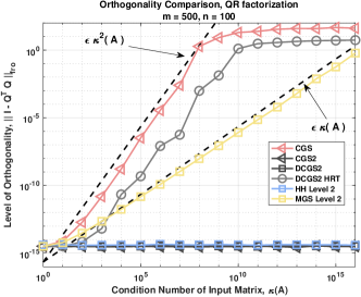
Both CGS and CGS2 are based upon matrix-vector operations. CGS applies a single projection, and then normalizes, requiring two separate steps. This projection step consists of two DGEMV kernel calls and one DDOT for the normalization. CGS suffers from at least an ${\cal O}(\varepsilon)\kappa^{2}(A)$ loss of orthogonality. CGS2 achieves ${\cal O}(\varepsilon)$ through two passes (see Figure 1). The additional projection within CGS2 accounts for one additional global reduction per iteration and an additional $4(m/p)j$ operations.

DCGS2 requires one reduction and employs matrix-matrix multiplies for the computation in a tall-and-skinny DGEMM. This leads to the higher sustained execution rate of DCGS2 (e.g. $2\times$ the GigaFlop/sec). In the context of Arnoldi, DCGS2 requires an additional $j^{2}$ flops at the $j$–th iteration. The additional cost is due to the Arnoldi representation trick described in Section 4. The representation error correction terms require an additional $n^{2}$ operations from a matrix-vector product with the Hessenberg matrix.

orth scheme	LOO	Proven
MGS Level 1	$\mathcal{O}(\varepsilon)\kappa(A)$	[18]
MGS Level 2	$\mathcal{O}(\varepsilon)\kappa(A)$	Conjectured
CGS	$\mathcal{O}(\varepsilon)\kappa^{2}(A)$	[7]
CGS2	$\mathcal{O}(\varepsilon)$	[7]
CGS2 (lagged norm)	$\mathcal{O}(\varepsilon)$	Conjectured
DCGS2-HRT	$\mathcal{O}(\varepsilon)\kappa^{2}(A)$	Conjectured
DCGS2 (QR)	$\mathcal{O}(\varepsilon)$	Conjectured
DCGS2 (Arnoldi)	$\mathcal{O}(\varepsilon)$	Conjectured

Table 3: Loss of Orthogonality (LOO).

6 Numerical Results

In this section, the numerical stability of the Arnoldi algorithm is investigated for the different orthogonalization schemes. The methodology for the numerical stability analysis is presented in Section 6.1 along with the experiments. The same methodology is employed in Section 7. Four stability metrics are examined,

1. representation error

2. loss of orthogonality

3. forward error in the eigenvalue solutions, $<$ threshold

4. dimension of converged invariant subspace, $<$ threshold

The metrics (1) and (2) are sufficient to analyze the stability of an orthogonalization scheme. However to give a broader perspective the metrics (3) and (4) are also examined. Additional metrics that can be considered are:

1. convergence of GMRES

2. achievable backward error of GMRES

3. number of eigenvalue-pairs (Ritz values) with a backward error $<$ threshold (see Hernandez et al. [16])

The convergence of GMRES and the achievable backward error are informative metrics, however, Paige et al. [5] proved that GMRES (with one right-hand side) only needs an $\mathcal{O}(\varepsilon)\>\kappa(B)$ LOO to converge. Therefore, GMRES is tolerant of “bad” orthogonalization schemes and is not a stringent enough test.

The number of eigenvalue-pairs with a backward error less than a threshold should not be used to assess the quality of an orthogonalization scheme because, for example, a scheme that always returns the same eigenvalue-pair $n$ times would score the highest possible score ($n$) according to this metric, while performing very poorly in any reasonable metric.

6.1 Manteuffel Matrix and experimental stability methodology

The matrix generated by “central differences” introduced by Manteuffel [20] is employed in a series of tests designed for the Krylov-Schur eigenvalue solver based upon DCGS2–Arnoldi. This matrix is convenient for computing the forward error solution because the explicit computation of each eigenvalue is possible, thus the comparison against a converged eigenvalue is possible. For $m\times m$ block diagonal matrices $M$ and $N$, where $M$ and $N$ have $k\times k$ sub-blocks such that $m=k^{2}$. ${M}$ is positive definite and ${N}$ is skew-symmetric. An explicit formulation of $M$ and $N$ is given in [20]. The Manteuffel matrix is expressed as the sum

$${A}=\frac{1}{h^{2}}{M}+\frac{\beta}{2h}{N}$$ (11)

where the matrix blocks and $k^{2}$ eigenvalues are generated by

$$\lambda_{\ell,j}=2\left[2-\sqrt{1-\left(\frac{\beta}{2}\right)^{2}}\left(\cos\left(\frac{\ell\pi}{L}\right)+\cos\left(\frac{j\pi}{L}\right)\right)\right],$$ (12)

For $\ell=1,\dots,k$ and $j=1,\dots,k$. As can be seen in (12), $\beta$ is a scalar that governs the spectrum of the eigenspace. $L$ is defined by the domain of the differential operator, $[0,L]\times[0,L]$ and $h=L\,/\,(k+1)$ is the discretization parameter. For the experiments within this section, $\beta=0.5$ and $L=k+1$ so that $h=1$ ($\beta\leq 2$ implies all eigenvalues are real). For $k=50$, relevant numerical metrics are summarized in Table 4. Here, ${V}$ and ${W}$ are the left and right eigenvectors. The Manteuffel matrix is employed to evaluate the convergence of Krylov-Schur.

$\|{A}\|_{2}$	$7.99$e$+00$
Cond(${A}$)	$3.32$e+$02$
Cond(${V}$)	$3.96$e$+11$
Cond(${W}$)	$3.74$e$+11$
$\|{A}^{T}{A}-{A}{A}^{T}\|_{F}/\|{A}\|_{F}^{2}$	$2.81$e$-04$
$\max_{i}$(  Cond($\;\lambda_{i}\;$) )	$1.46$e$+10$
$\min_{i}$(  Cond($\;\lambda_{i}\;$) )	$2.38$$+02$

Table 4: Differential operator specs for $k=50$, $m=k^{2}=2500$.

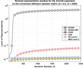
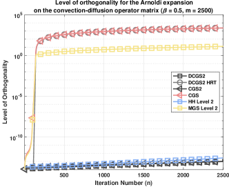
The Arnoldi residual and error metrics employed herein are described in Hernández et al. [21]. Figure 4 displays the loss of orthogonality $\|\>I_{j-1}-{Q}_{1:j-1}^{T}{Q}_{1:j-1}\>\|_{F}$, while Figure 3 is a plot of the Arnoldi relative representation error, from (1)

$$RRE(j)=\frac{\left\|\>{AQ}_{1:j-2}-{Q}_{1:j-1}H_{1:j-1,1:j-2}\>\right\|_{F}}{\|{A}\|_{F}}.$$

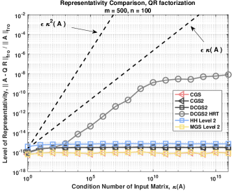
Each of the algorithms, except for the DCGS2-HRT presented in [16], achieve machine precision level relative error. Figure 4 displays the loss of orthogonality for each scheme. It was noted earlier that CGS exhibits an $\mathcal{O}(\varepsilon)\kappa^{2}(A)$ loss of orthogonality. The plot illustrates that DCGS2-HRT follows CGS while the other algorithms construct orthonormal columns to the level of machine precision.

Figure 3: Representation error.

Figure 4: Loss of orthogonality.

Figure 5: Number of eigenvalues computed with $10^{-7}$ absolute error.

Figure 6: Dimension of invariant subspace computed.

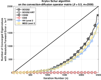
The results from a Krylov-Schur eigenvalue experiment to evaluate the convergence properties of the different Arnoldi algorithms are plotted in Figure 5. The solver relies upon the Schur decomposition of the Hessenberg matrix $H_{n}$ generated in the Arnoldi expansion. To assess the convergence rates, the Arnoldi residual (13) is compared to the absolute error tolerance. The approximate eigenvector (or Ritz vector) associated with the eigenvalue $\lambda_{i}$ is defined by $z_{i}=V_{n}\>y_{i}$, where $y_{i}$ is the corresponding eigenvector of $H_{n}$, see [16].

$$\|\>(\>A-\lambda_{i}\>I\>)\>z_{i}\>\|_{2}=|H_{n+1,n}|\>|\>e_{n}^{T}y_{i}\>|\><\>\text{tol}$$ (13)

where ${\rm tol}=1$e$-7$. If this threshold is satisfied, the iteration is considered to have found an invariant subspace and the associated diagonal element in the Schur triangular matrix $T_{l,l}$ is an eigenvalue. The representation error and loss of orthogonality can be easily computed. It is important to note if these quantities are not close to machine precision, a converged invariant subspace has not been found. After the size of the invariant subspace has been found, the $k^{2}$ eigenvalues from the formula in (12) are computed and compared with the “converged” eigenvalues in the Schur triangular matrix $T$. In addition, rather than computing the same eigenvalue twice, the multiplicity is obtained to determine if the Krylov-Schur algorithm has computed the same eigenvalue, or unique eigenvalues in the decomposition. The exact multiplicity of any given eigenvalue was always found.

The plot in Figure 5 displays the number of converged eigenvalues at each step $m$ of the Arnoldi algorithm according to the absolute forward error $|\lambda_{i}-T_{l,l}|<\text{tol}$, where $\text{tol}=1e-7$. In practice, at each iteration $n$, for each $l$ from $1$ to $n$, the $\lambda_{i}$ are scanned for each $i$ closest to $T_{l,l}$, which has not been found for a previous $l$, and which satisfies the tolerance is selected. Our code will return an error flag if an iteration returns more eigenvalues than the expected multiplicity. The flag was never triggered during our experiments. At iteration $n$, at most $n$ eigenvalues are found and these correspond to the solid black line. There are three reasons why the number of eigenvalues found is not $n$. First, the eigenvalues must be converged. At step $n$, in exact arithmetic, all eigenvalues would have been found. For step $n<m$, the number of eigenvalues found is between $0$ and $n$. Second, the forward error is sensitive to the condition number of the eigenvalues. Some eigenvalues have condition number of the order $1$e$+10$, (see Table 4), therefore, using $\varepsilon=2.2$e$-16$ accuracy, our algorithms are not expected to find all eigenvalues at iteration $m=2,500$. The maximum number of eigenvalues found is about $2,100$ with CGS2 and DCGS2 methods. This condition number problem is present at any restart $n$ and is intrinsic when using a forward error criteria. Third, the Arnoldi–$QR$ factorization could have errors in fundamental quantities such that the loss of orthogonality and representation error are large. This may affect the number of eigenvalues found at iteration $n$.

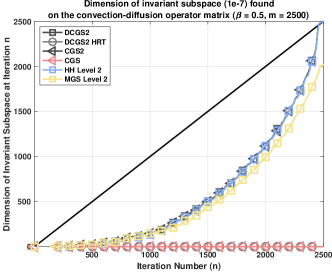
Figure 6 displays, at each restart $n$, the size of the invariant subspace found. None of the methods can follow this line, but as the full Arnoldi expansion of the Manteuffel matrix is approached, any scheme that maintains orthogonality can continually find new eigenvalues, or new directions to search. Comparing both plots illustrates that in practice, when eigenvalues are not known, looking at the size of the invariant subspace can be a good metric. Note that between the two plots, there is a small gap for the error formula at a restart of $m=2500$, where this gap is not present in the invariant subspace plot. The different Arnoldi variants cannot find all of the invariant subspaces, which is due to the condition number of the eigenvalues. Comparing the different $QR$ factorization schemes and the invariant subspace found, although it loses orthogonality, Arnoldi with MGS can still find new search directions. Arnoldi–$QR$ based on Householder (HH), CGS2 and DCGS2, can find a subspace that spans the entire space, but for this matrix MGS still performs well and generates a subspace size close to 2000.

6.2 Matrix Market

The Arnoldi–$QR$ factorization algorithms are now compared for matrices gathered from the Suite-Sparse collection maintained by Tim Davis at Texas A&M University [22]. A total of 635 matrices were chosen by the following criteria: (1) number of nonzeros $<\;500,000$, (2) the matrix is REAL, (3) the matrix is UNSYMMETRIC and (4) the number of columns and rows $>\;100$. The Krylov basis is computed for each of the 635 matrices in the collection. The representation error and loss of orthogonality are computed for every 5 columns until 75 (making sure the dimension of any matrix is not exceeded). Meaning the restart in an Arnoldi expansion varies from $n=5$ to $n=75$ in increments of $5$.

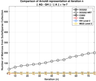
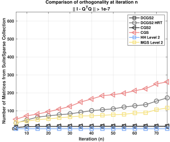
Figures 7 and 8 display these metrics for each of the schemes. At each iteration the tolerance is set to $1$e$-7$. If the representation error or loss of orthogonality is above this threshold the matrix is flagged. The $y$-axis represents the total number of matrices above the given threshold and the $x$-axis indicates the Krylov subspace dimension (restart $m$) employed by the Arnoldi expansion.

Figure 8 clearly indicates that Krylov vectors generated using CGS and MGS lose orthogonality at different rates. It is observed that the DCGS2-HRT curve falls between these. For the Manteuffel matrix, DCGS2-HRT appears to perform more like CGS and lies somewhere in between. It is important to note, in Figure 7, that DCGS2-HRT does not maintain a low representation error for the Arnoldi expansion. This is also apparent in Figure 2.

With a restart of $n=75$, these metrics are plotted in Table 5. The additional metric displayed is the size of the invariant subspace found, described in Section 6.1.

Orth.	Repres	LOO	Invariant
scheme	$<$ $1$e$-7$	$<$ $1$e$-7$	Subspace
DCGS2	631	621	9844
DCGS2 HRT	435	463	7168
CGS2	635	622	9677
CGS	635	374	8370
HH Level 2	635	635	9783
MGS Level 2	634	519	9580

Table 5: $n$ = 75; $\text{tol}=1$e$-7$; Suite-Sparse matrices

Figure 7: Representation error for Suite-Sparse matrices.

Figure 8: Loss of Orthogonality for Suite-Sparse matrices.

7 Parallel Performance Results

Parallel performance results are now presented for the Summit Supercomputer at Oak Ridge National Laboratory. Each node of Summit consists of two 22-core IBM Power 9 sockets and six NVIDIA Volta 100 GPUs. CGS2 and DCGS2 were implemented and tested using the Trilinos-Belos iterative solver framework [13, 23]. Therefore, although NVIDIA V100 results are presented here, the implementation is portable to different hybrid node architectures with a single code base.

To summarize, DCGS2 achieves faster compute times than CGS2 for two reasons. First, the former employs either matrix-vector or matrix-matrix kernels, which provide greater potential for data reuse. For tall-and-skinny matrices, employed by DGEMV and DGEMM, compute time is often limited by data movement, and matrix-matrix type kernels often achieve faster execution rates. Therefore, DCGS2 is faster than CGS2, even on a single GPU. Second, on multiple GPUs, the low-synch algorithm decreases the number of global-reductions. Therefore, a greater speedup is achieved on a large number of GPUs. In this section, the execution rates on a single and multiple GPUs are compared.

7.1 Single GPU Performance

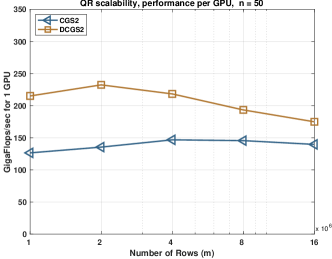
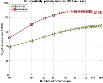
Figure 9 provides the execution rates in GigaFlops/sec of the main computational kernels on a single GPU, with an increasing number of rows or columns, as reported in 9(a) and columns 9(b) respectively. Within the plot,

• MvTransMv computes the dot-products, e.g., DGEMV to compute $S_{1:j-1,j}=Q_{1:j-1}^{T}a_{j}$ in CGS2 or DGEMM to compute $[\>Q_{1:j-2},\>w_{j-1}]^{T}[\>w_{j-1},\>a_{j}\>]$ in DCGS2.

• MvTimesMatAddMv updates the vectors by applying the projection, e.g., DGEMV to compute $w_{j}=q_{j}-Q_{1:j-1}\>S_{1:j-1,j}$ in DCGS2 or DGEMM to compute

  $$\left[\>u_{j-1},\>w_{j}\>\right]=\left[\>w_{j-1},\>a_{j}\>\right]-Q_{1:j-2}\>\left[\>C_{1:j-2,j-1},\>S_{1:j-1,j}\>\right]$$

• MvDot computes DDOT product of two vectors, and is used to compute the normalization factor $\alpha_{j-1}=\|u_{j}\|_{2}$.

Orthog	Number of rows, $n$, in millions
Scheme	$1$	$2$	$4$	$8$	$16$
DCGS2
MVTimes GF/s	300.3	319.1	302.3	320.3	331.4
MVTrans GF/s	201.4	211.8	191.4	150.2	126.8
Total GF/s	215.1	232.3	218.2	193.3	174.8
CGS2
MVTimes GF/s	132.0	136.4	153.4	163.8	169.5
MVTrans GF/s	128.5	141.0	146.4	135.3	122.2
Total GF/s	126.4	135.4	146.7	145.5	139.6

(a) Fixed number of columns $n=50$.

Orthog	Number of columns, $n$
Scheme	$100$	$120$	$140$	$160$	$180$
DCGS2
MVTimes GF/s	353.7	362.8	369.8	375.6	379.7
MVTrans GF/s	169.2	164.3	160.3	158.7	155.6
Total GF/s	221.2	219.8	218.4	218.5	216.6
CGS2
MVTimes GF/s	182.1	186.9	190.7	193.1	195.7
MVTrans GF/s	152.0	153.6	153.4	153.3	153.2
Total GF/s	163.8	167.1	168.6	169.7	170.8

(b) Fixed number of rows $m=5$e$+6$.

Figure 9: Execution rate (GigaFlops/sec) of BLAS kernels (1 node, 1 GPU).

Memory bandwidth utilization is a predictor of performance. For example, at the $j$–th iteration of CGS2, MvTransMV reads the $m\times(j-1)$ matrix $Q_{1:j-1}$ and the input vector $a_{j}$ of length $m$, then writes the result back to the output vector $S_{1:j-1,j}$, while performing $(2m-1)\times(j-1)$ flops with two flops per read, assuming the vectors remain in caches, or two flops per two reads and one write with a read-write of vector elements for each multiply-add. Thus, on the V100 with a memory bandwidth of 800 GB/s, 200 GigaFlops/sec is expected from this kernel in double precision. Figures 10 and 11 display kernel compute times on one Summit node using one GPU as the number of rows or columns is varied.

Note that DCGS2 combines two MvTransMv calls with a single input and output vector into a call to MvTimesMatAddMv with two input and output vectors. This can double the potential peak speed (i.e. the $m\times(j-1)$ matrix is read only once to perform four flops per read). Figure 9 indicates that for a large number of rows or columns, that DCGS2 increases the execution rate by up to $1.7$ and $1.4\times$, respectively..

Figure 10: Execution rate (GigaFLops/sec, 1 GPU). $n=50$ columns.

Figure 11: Execution rate (GigaFlops/sec, 1 GPU). $m=25$e$+6$ rows.

7.2 Strong-Scaling Performance

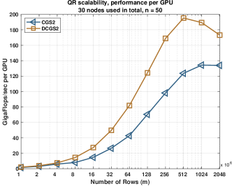
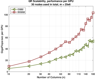
The speedups obtained by DCGS2 for the two main kernels are presented in Tables 6, 7 and 8, while Figures 13 and 14 and displays the GigaFlops/sec execution rate achieved by the kernels on 30 nodes, using 6 GPUs per node. Figures 15 and 16 represent a strong-scaling study and display the time to solution while varying the number of GPUs for a fixed matrix size. One run or trial for each node count was employed for the algorithms in order to collect the performance data on Summit.

• Table 6 displays the speedup (ratio of DCGS2 to CGS2 compute time) for MvTransMv. Because DCGS2 employs fewer global reductions, as the number of GPUs increases, the speedup obtained by MvTransMv increases, reaching up to $2.20\times$ faster times on 192 GPUs.

• Table 7 displays the speedup for the MvTimesMatAddMv kernel. DCGS2 merges two MvTransMv calls into one MvTimesMatAddMv and achieves $2\times$ speedup on a single GPU. With more GPUs, the number of local rows and speedup decrease. However, the compute time is dominated by the MvTimesMatAddMv kernel.

Table 8 displays the speedup obtained by DCGS2, when varying the number of rows. By combining matrix-vector products with global reductions, the speedup obtained by DCGS2 in some instances was significant, up to $3.6\times$ faster.

Figures 15 and 16 display the time to solution for the GMRES linear solvers. The latter achieves improved strong scaling due to the merged MvTimesMatAddMv kernel.

Orthog	Number of rows, $n$, in millions
Scheme	$128$	$256$	$512$	$1024$	$2048$
DCGS2
MVTimes GF/s	194.2	248.9	285.9	312.5	324.2
MVTrans GF/s	129.4	170.4	179.9	154.1	128.6
Total GF/s	124.3	168.9	195.4	189.4	173.2
CGS2
MVTimes GF/s	99.6	126.6	145.1	158.9	167.1
MVTrans GF/s	73.9	100.8	124.9	128.4	119.3
Total GF/s	42.8	98.2	123.7	134.3	133.9

(a) Fixed number of columns $n=50$. GigaFlops/sec

Orthog	Number of columns, $n$
Scheme	$100$	$120$	$140$	$160$	$180$
DCGS2
MVTimes GF/s	121.6	135.5	151.2	159.7	168.9
MVTrans GF/s	61.1	76.9	89.1	89.1	107.6
Total GF/s	61.4	74.4	84.4	90.1	103.4
CGS2
MVTimes GF/s	122.2	95.2	101.3	99.3	90.4
MVTrans GF/s	38.1	39.4	49.6	56.5	52.6
Total GF/s	36.4	38.9	47.7	54.5	53.4

(b) Fixed number of rows $n=25$e$+6$. GigaFlops/sec

Figure 12: Execution rate (GigaFlops/sec) of BLAS kernels (30 nodes, 6 GPUs per node ).

Figure 13: Execution rate per node (30 nodes, 6 GPUs per node).

Figure 14: Execution rate per node (30 nodes, 6 GPUs per node).

	Number of rows, $n$
# GPUs	$1$e$+6$	$5$e$+6$	$10$e$+6$	$25$e$+6$	$50$e$+6$
6	1.7	1.6	1.6	1.3	1.1
12	1.9	1.8	1.7	1.5	1.3
24	2.1	1.7	1.7	1.6	1.5
48	2.1	1.9	1.9	1.8	1.6
96	2.0	2.1	4.0	1.8	1.8
192	2.2	2.1	2.3	2.1	2.2

Table 6: Speedup of DCGS2 over CGS2 for MvTransMv and MvDot.

	Number of rows, $n$
# GPUs	$1$e$+6$	$5$e$+6$	$10$e$+6$	$25$e$+6$	$50$e$+6$
6	0.8	2.0	2.0	1.9	2.0
12	1.9	2.0	1.9	2.0	1.9
24	1.3	0.9	1.2	2.0	2.0
48	1.1	0.9	0.9	1.9	2.0
96	1.1	0.8	5.2	1.1	1.3
192	0.9	0.7	0.7	0.9	1.3

Table 7: Speedup of DCGS2 over CGS2 for MvTimesMatAddMv.

	Number of rows, $n$
# GPUs	$1$e$+6$	$5$e$+6$	$10$e$+6$	$25$e$+6$	$50$e$+6$
6	1.1	1.6	1.7	1.5	1.3
12	1.1	1.8	1.7	1.6	1.5
24	1.1	1.5	1.8	1.7	1.6
48	1.2	1.1	1.8	1.8	1.7
96	1.2	1.3	4.0	1.8	1.8
192	1.4	1.3	1.7	1.9	2.1

Table 8: Overall speedup of DCGS2 over CGS2.

Figure 12 displays the GigaFlops/sec execution rates obtained by CGS2 and DCGS2, along with the BLAS kernels for a fixed matrix size ($m=25$e$+6$ and $n=50$). The MvTransMv operation requires a global reduce, while the DGEMM operations do not require communication. DCGS2 always outperforms CGS2 in these runs. MvTimesMatAddMv perform similarly for both schemes on 96 and 192 nodes. CGS2 exhibits an increase in speed that matches DCGS2. For a large number of rows or columns, DCGS2 obtains about $66$ GigaFlops/sec per node at 192 nodes or about 6% of the single GPU sustained execution rate of 200 GigaFlops/sec.

Figure 15: Time to solution of GMRES. $m=750^{3}$, $n=100$ (256 nodes, 6 GPUs per node).

Figure 16: Time to solution of GMRES. $m=1000^{3}$, $n=100$ (256 nodes, 6 GPUs per node).

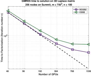
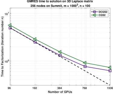
Figures 15 and 16 are strong scaling experiments for the 3D Laplace equation with dimension $m=750^{3}$ and $m=1000^{3}$. The simulations employ from 8 to 256 Summit compute nodes. The GMRES solver is run for one trial for each of the node counts using 6 GPUs per node, in non-dedicated runs on Summit. A fixed number of $n=100$ iterations are performed, without a restart, and a preconditioner is not applied. Clearly, the DCGS2-GMRES yields lower run times and exhibits better strong-scaling characteristics.

8 Conclusion

For distributed-memory computation, two passes of classical Gram-Schmidt (CGS2) was the method of choice for Krylov solvers requiring machine precision level representation errors and loss of orthogonality. However, the algorithm requires three global reductions for each column of the $QR$ decomposition computed and thus the strong-scaling behavior can deviate substantially from linear as the number of MPI ranks increases on Exascale class supercomputers such as the ORNL Summit. In this paper, a new variant of CGS2 that requires only one global reduction per iteration was applied to the Arnoldi-$QR$ algorithm. Our numerical results have demonstrated that DCGS2 obtains the same loss of orthogonality and representation error as CGS2, while our strong-scaling studies on the Summit supercomputer demonstrate that DCGS2 obtains a speedup of $2\times$ faster compute time on a single GPU, and an even larger speedup on an increasing number of GPUs, reaching $2.2\times$ lower execution times on 192 GPUs. The impact of DCGS2 on the strong scaling of Krylov linear system solvers is currently being explored, and a block variant is also being implemented following the review article of Carson et al. [15]. The software employed for this paper is available on GitHub.

References

- [1] T. R. Stones, Let it bleed (1969).
- [2] Y. Saad, M. H. Schultz, GMRES: A generalized minimal residual algorithm for solving nonsymmetric linear systems, SIAM Journal on scientific and statistical computing 7 (3) (1986) 856–869.
- [3] G. W. Stewart, A Krylov–Schur algorithm for large eigenproblems, SIAM Journal on Matrix Analysis and Applications 23 (3) (2001) 601–614.
- [4] L. Giraud, J. Langou, M. Rozložník, On the loss of orthogonality in the Gram-Schmidt orthognalization process, Computers and Mathematics with Applications 50 (2005) 1069–1075. doi:doi:10.1016/j.camwa.2005.08.009.
- [5] C. C. Paige, M. Rozložník, Z. Strakoš, Modified Gram-Schmidt (MGS), least squares, and backward stability of MGS-GMRES, SIAM Journal on Matrix Analysis and Applications 28 (1) (2006) 264–284. doi:10.1137/050630416.
- [6] A. Bienz, W. Gropp, L. Olson, Node-aware improvements to allreduce, in: Proceedings of the 2019 IEEE/ACM Workshop on Exascale MPI (ExaMPI), Association for Computing Machinery, 2019, pp. 1–10.
- [7] L. Giraud, J. Langou, M. Rozložník, J. van den Eshof, Rounding error analysis of the classical Gram-Schmidt orthogonalization process, Numerische Mathematik 101 (1) (2005) 87–100.
- [8] A. Smoktunowicz, J. L. Barlow, J. Langou, A note on the error analysis of classical Gram-Schmidt, Numerische Mathematik 105 (2) (2006) 299–313.
- [9] C. C. Paige, The effects of loss of orthogonality on large scale numerical computations, in: Proceedings of the International Conference on Computational Science and Its Applications, Springer-Verlag, 2018, pp. 429–439.
- [10] B. N. Parlett, The Symmetric Eigenvalue Problem, Society for Industrial and Applied Mathematics, 1998. doi:10.1137/1.9781611971163.
- [11] K. Swirydowicz, J. Langou, S. Ananthan, U. Yang, S. Thomas, Low synchronization Gram-Schmidt and generalized minimal residual algorithms, Numerical Linear Algebra with Applications 28 (2020) 1–20.
- [12] V. Frayssé, L. Giraud, H. K. Aroussi, On the influence of the orthogonalization scheme on the parallel performance of GMRES, Tech. Rep. TR-PA-98-07, CERFACS (1998).
- [13] E. Bavier, M. Hoemmen, S. Rajamanickam, H. Thornquist, Amesos2 and Belos: Direct and iterative solvers for large sparse linear systems, Scientific Programming 20 (3) (2012) 241–255.
- [14] S. K. Kim, A. T. Chronopoulos, An efficient parallel algorithm for extreme eigenvalues of sparse nonsymmetric matrices, International Journal of Supercomputer Applications 6 (1) (1992) 98–111.
- [15] E. Carson, K. Lund, M. Rozložník, S. Thomas, An overview of block Gram-Schmidt methods and their stability properties (2020). arXiv:2010.12058.
- [16] V. Hernández, J. Román, A. Tomas, Parallel Arnoldi Eigensolvers with enhanced scalability via global communications rearrangement, Parallel Computing 33 (2007) 521–540.
- [17] I. Yamazaki, S. Thomas, M. Hoemmen, E. G. Boman, K. Świrydowicz, J. J. Elliott, Low-synchronization orthogonalization schemes for -step and pipelined Krylov solvers in Trilinos, in: Proceedings of the 2020 SIAM Conference on Parallel Processing for Scientific Computing, SIAM, 2020, pp. 118–128. doi:10.1137/1.9781611976137.11.
- [18] A. Björck, Solving least squares problems by Gram–Schmidt orthogonalization, BIT 7 (1967) 1–21.
- [19] E. Carson, K. Lund, M. Rozložník, The stability of block variants of classical Gram-Schmidt, Tech. Rep. 6-2021, Czech Academy of Sciences (2021).
- [20] T. A. Manteuffel, Adaptive procedure for estimating parameters for the nonsymmetric Tchebychev iteration, Numerische Mathematik 31 (2) (1978) 183–208.
- [21] V. Hernández, J. Román, A. Tomas, V. Vidal, Krylov-Schur methods in SLEPc, Tech. Rep. SLEPc Technical Report STR-7, University of Valencia (2007).
- [22] T. A. Davis, Y. Hu, The university of florida sparse matrix collection, ACM Trans. Math. Softw. 38 (1) (Dec. 2011). doi:10.1145/2049662.2049663.
- [23] M. Heroux, et. al., An overview of the Trilinos project, ACM Trans. Math. Softw. (2005).