Two-Stage Gauss–Seidel Preconditioners and Smoothers for Krylov Solvers on a GPU cluster

Abstract

Gauss-Seidel (GS) relaxation is often employed as a preconditioner for a Krylov solver or as a smoother for Algebraic Multigrid (AMG). However, the requisite sparse triangular solve is difficult to parallelize on many-core architectures such as graphics processing units (GPUs). In the present study, the performance of the sequential GS relaxation based on a triangular solve is compared with two-stage variants, replacing the direct triangular solve with a fixed number of inner Jacobi-Richardson (JR) iterations. When a small number of inner iterations is sufficient to maintain the Krylov convergence rate, the two-stage GS (GS2) often outperforms the sequential algorithm on many-core architectures. The GS2 algorithm is also compared with JR. When they perform the same number of flops for SpMV (e.g. three JR sweeps compared to two GS sweeps with one inner JR sweep), the GS2 iterations, and the Krylov solver preconditioned with GS2, may converge faster than the JR iterations. Moreover, for some problems (e.g. elasticity), it was found that JR may diverge with a damping factor of one, whereas two-stage GS may improve the convergence with more inner iterations. Finally, to study the performance of the two-stage smoother and preconditioner for a practical problem, these were applied to incompressible fluid flow simulations on GPUs.

1 Introduction

Solving large sparse linear systems of the form $A\mathbf{x}=\mathbf{b}$ is a basic and fundamental component of physics based modeling and simulation. For solving these large linear systems, Krylov methods such as the Generalized Minimal Residual (GMRES) [1] are widely adopted. To accelerate the convergence rate of the Krylov solver, Gauss-Seidel (GS) relaxation is often employed either as the preconditioner for a Krylov solver directly, or as the smoother in a $V$–cycle of a multigrid preconditioner.

In this study, GS relaxation is examined in the context of the Trilinos [2] and hypre [3] software packages. On a distributed-memory computer, both Trilinos and hypre implement a hybrid variant [4] of Gauss-Seidel iteration where the boundary information is exchanged to compute the residual vector, but then each MPI process applies a fixed number of local relaxation sweeps independently. This hybrid block-Jacobi type algorithm is shown to be effective and scalable for many problems (i.e., the iteration counts stay roughly constant with increasing subdomain count). However, to perform the local relaxation, each process still requires a local sparse-triangular solve, which is inherently challenging to parallelize on the GPU architecture. Although several techniques have been proposed to improve the time to solution, the local sparse-triangular solve recurrence could still be the bottleneck for scalability of the solver, and in turn, of the entire simulation.

In the present study, a two-stage iterative variant of the GS relaxation algorithm is proposed as an alternative to the sequential algorithm based on a triangular solve. In the two-stage algorithm, henceforth called GS2, the triangular solve is replaced with a fixed number of Jacobi-Richardson inner relaxation sweeps. Each inner sweep carries out the same number of floating-point operations (flops) as the triangular solve, but is based on a sparse matrix vector multiply (SpMV), which is much easier to parallelize and can be much faster than the sparse-triangular solve on a GPU. Consequently, when a small number of inner iterations is needed to maintain the quality of the preconditioner, GS2 can surpass the sequential approach.

The GS2 is also compared with the Jacobi-Richardson (JR) iteration, which is a special case of the GS2 iteration without inner iterations. Our results using Laplace and elasticity problems, together with the Suite-Sparse matrix collection, demonstrate that when GS2 and JR are applied as stand-alone solvers and execute the same number of SpMVs, then JR converges asymptotically faster. Consequently, GMRES often converges with fewer iterations, and with a shorter time to solution. In contrast, the JR sweep computes the SpMV with the full matrix, while the inner JR sweep of GS2 applies the SpMV with a triangular matrix. When the two methods execute about the same number of flops for SpMV (e.g. three JR sweeps compared to two GS2 sweeps with one inner JR sweep), the GS2 preconditioner may lead to faster convergence as measured by the iteration counts, and in some cases, the time to solution. Moreover, for some problems (e.g. elasticity), JR may diverge, while GS2 can improve the convergence using additional inner iterations (if the inner iteration converges).

Lower precision floating point arithmetic is also investigated as an alternative approximation for the preconditioner. In experiments with a conjugate gradient (CG) solver and symmetric version of GS2 (SGS2), high accuracy was not required for the outer SGS nor the inner JR iterations. Thus, the low-precision inner iteration can be applied to maintain the convergence rate of the Krylov solver, while reducing the compute time by a factor of $1.4\times$.

Finally, to study the effectiveness of the GS2 preconditioner and smoother in a practical setting, they are applied in Nalu-Wind [5] for incompressible fluid flow simulations. In the context of a time-split, pressure-projection scheme within nonlinear Picard iterations, GS is used as a preconditioner for GMRES when solving the momentum problems, and GS, or Chebyshev, is applied as a smoother in algebraic multigrid (AMG) when solving pressure problems. For representative wind-turbine incompressible flows, simulation results are reported for an atmospheric boundary layer (ABL) precursor simulation on a structured mesh. Our strong-scaling results on the Oak Ridge Leadership Computing Facility (OLCF) supercomputer Summit demonstrate that the GS2 preconditioner requires just one inner sweep to obtain a similar convergence rate compared to the sequential algorithm, and thus it achieves a faster time to solution. In addition, the GS2 smoother was often as effective as a Chebyshev polynomial smoother.

2 Related Work

Because a sparse triangular solver is a critical kernel in many applications, significant effort has been devoted to improving the performance of a general-purpose sparse triangular solver for both CPUs [6, 7, 8] and GPUs [9, 10, 11, 12, 13]. For example, the traditional parallel algorithm is based upon level-set scheduling, derived from the sparsity structure of the triangular matrix and is also implemented in the cuSPARSE [14] library. Independent computations proceed within each level of the tree. In the context of Gauss-Seidel relaxation, Deveci et. al.  implemented a multi-threaded triangular solver, based on multi-coloring [15]. Multi-coloring exposes parallelism but may increase the iteration count for Krylov solvers in certain problems. Another fine-grain algorithm is based on partial in-place inversion of products of elementary matrices after re-ordering to prevent fill-in. Here, the triangular solve is applied as a sequence of matrix-vector multiplies [16]. When the input matrices have a denser non-zero pattern arising from a super-nodal factorization, a block variant could exploit the GPU more effectively [17]. Overall, the sparsity pattern of the triangular matrix may limit the amount of parallelism available for the solver to fully utilize many-core architectures, especially when compared with other cuBLAS [18] and cuSPARSE operations, including a matrix-vector multiply.

Two-stage nested iteration, for which GS2 is a special case, has been studied in a series of articles by Frommer and Szyld [19, 20, 21, 22]. Unlike the triangular solver algorithm, the two-stage iteration can be implemented using only (sparse or dense) matrix-vector products and vector updates. As stated previously, these operations can be implemented very efficiently on multi-core architectures. The application of Jacobi iterations to solve sparse triangular linear systems for ILU preconditioners, rather than forward or backward recurrence, was also recently proposed by Chow et. al. [23].

3 Gauss-Seidel Algorithms

To solve a linear system $A\mathbf{x}=\mathbf{b}$, the Gauss-Seidel (GS) iteration is based on the matrix splitting $A=L+D+U$, where $L$ and $U$ are the strictly lower and upper triangular parts of the matrix $A$, respectively. Then, the sequential GS iteration updates the solution based on the following recurrence,

(1) $$\mathbf{x}_{k+1}:=\mathbf{x}_{k}+M^{-1}\mathbf{r}_{k},\quad k=0,1,2,\ldots$$

where $\mathbf{r}_{k}=\mathbf{b}-A\mathbf{x}_{k}$, and $M=L+D$, $N=-U$ or $M=U+D$ for the forward or backward sweeps, respectively. The iteration matrix is $G=I-M^{-1}A$ and when (1) converges, $\rho(G)<1$, (c.f. Theorem 4.1 of Saad [24]). When the matrix $A$ is symmetric, a symmetric variant of GS (SGS) performs the forward followed by the backward sweep to maintain the symmetry of the matrix operation. In the remaining discussions, we refer to 1 as the non-compact form.

To avoid explicitly forming the inverse $M^{-1}$ in (1), a sparse triangular solve is applied to the current residual vector $\mathbf{r}_{k}$. On a distributed-memory computer, both Trilinos and hypre distribute the matrix and the vectors in a 1–D block row fashion among the MPI processes (the local matrix on the $p$-th MPI process is rectangular, consisting of the square diagonal block $A^{(p)}$ for the rows owned by the MPI process and the off-diagonal block $E^{(p)}$ for the off-process columns. On each MPI rank, hypre stores the local diagonal block $A^{(p)}$ separately from the off-diagonal block $E^{(p)}$, whereas Trilinos stores them as a single matrix). The standard parallel sparse triangular solve is based on level-set scheduling [6, 7] and will compute the independent set of the solution elements in parallel at each level of scheduling. Unfortunately, the sparsity structure of the triangular matrix may limit the parallelism that the solver can exploit (e.g. the sparsity structure may lead to a long chain of dependencies with a small number of solution elements that can be computed at each level). In addition, at the start of each level, neighboring processes need to exchange the elements of the solution vector on a processor boundary for updating their local right-hand-side vectors.

To improve scalability, both Trilinos and hypre implement a hybrid variant of GS relaxation [4], where the neighboring processes first exchange the elements of the solution vector on the boundary, but then each process independently applies the local relaxation. Hence, $M$ is a block diagonal matrix with each diagonal block $M^{(p)}$ corresponding to the triangular part of the local diagonal block $A^{(p)}$ on each process. The method may be considered as an inexact block Jacobi iteration, where the local problem associated with the diagonal block is solved using a single GS iteration. Furthermore, in hypre, each process may apply the multiple local GS sweeps for each round of the neighborhood communication. With this approach, each local relaxation updates only the local part of the vector $\mathbf{x}_{k+1}$ (during the local relaxation, the non-local solution elements on the boundary are not kept consistent among the neighboring processes). Hence, the local GS relaxation, on the $p$-th MPI rank, iterates to solve the local linear system $A^{(p)}\mathbf{x}^{(p)}_{k+1}=\widehat{\mathbf{b}}_{t}^{(p)}$ where $\widehat{\mathbf{b}}_{t}^{(p)}:=\mathbf{b}^{(p)}-E^{(p)}\mathbf{y}_{t}^{(p)}$ and $\mathbf{y}_{t}^{(p)}$ is the non-local part of the current solution vector exchanged before the start of the local GS iteration. In contrast, Trilinos currently computes the global residual vector for each local iteration through neighborhood communication. The only exception is the symmetric GS relaxation that applies both the forward and backward iterations after a single round of neighborhood communication.

In this hybrid GS, each process can apply the local relaxation independently, improving the scalability compared to the global sparse triangular solve. This hybrid algorithm is shown to be effective and scalable for many problems [4] (e.g. the Krylov iteration count, when combined with this hybrid GS preconditioner, remains roughly constant with an increasing process count). However, to implement the local iteration, each process must still perform a local sparse triangular solve, which can be difficult to parallelize on many-core architectures.

4 Two-stage Gauss-Seidel Algorithms

In the present study, a two-stage GS relaxation, with a fixed number of “inner” stationary iterations, approximately solves the triangular system with $M$,

(2) $$\widehat{\mathbf{x}}_{k+1}:=\widehat{\mathbf{x}}_{k}+\widehat{M}^{-1}(\mathbf{b}-A\widehat{\mathbf{x}}_{k}),\quad k=0,1,2,\ldots$$

where $\widehat{M}^{-1}$ represents the approximate triangular system solution, i.e. $\widehat{M}^{-1}\approx M^{-1}$.

A Jacobi-Richardson (JR) iteration is employed for the inner iteration. More specifically, $\mathbf{g}_{k}^{(j)}$ denotes the approximate solution from the $j$–th inner JR iteration at the $k$–th outer GS iteration. The initial solution is chosen to be the diagonally-scaled residual vector,

(3) $$\mathbf{g}_{k}^{(0)}=D^{-1}\mathbf{r}_{k},$$

and the $(j+1)$–st JR iteration computes the solution by the recurrence

(4) $$\mathbf{g}_{k}^{(j+1)} := \mathbf{g}_{k}^{(j)}+D^{-1}(\mathbf{r}_{k}-(L+D)\mathbf{g}_{k}^{(j)})$$

(5) $$= D^{-1}(\mathbf{r}_{k}-L\mathbf{g}_{k}^{(j)}).$$

Figure 1 displays the SGS2 algorithm, the symmetric extension of GS2.

for $t=1,2,\dots,n_{t}$ do 1. // exchange interface elements of current solution for $k=1,2,\dots,n_{k}$ do 2. // compute new residual vector for forward sweep $\mathbf{r}_{k}:=\mathbf{b}-U\mathbf{x}_{k}$ 3. // perform local inner Jacobi iteration $\mathbf{g}^{(0)}_{k}:=D^{-1}\mathbf{r}_{k}$ for $j=0,1,\dots,n_{j}-1$ do $\mathbf{g}^{(j+1)}_{k}:=D^{-1}(\mathbf{r}_{k}-L\mathbf{g}^{(j)}_{k})$ end for 4. // update solution vector $\mathbf{x}_{k+1}:=\mathbf{x}_{k}+\mathbf{g}^{(s)}_{k}$ 5. // compute new residual vector for backward sweep $\mathbf{r}_{k}:=\mathbf{b}-L\mathbf{x}_{k}$ 6. // perform local inner Jacobi iteration $\mathbf{g}^{(0)}_{k}:=D^{-1}\mathbf{r}_{k}$ for $j=0,1,\dots,s$ do $\mathbf{g}^{(j+1)}_{k}:=D^{-1}(\mathbf{r}_{k}-U\mathbf{g}^{(j)}_{k})$ end for 7. // update solution vector $\mathbf{x}_{k+1}:=\mathbf{x}_{k}+\mathbf{g}^{(s)}_{k}$ end for end for

Figure 1: Pseudo-code of two-stage hybrid Symmetric Gauss-Seidel iteration, using Jacobi-Richardson as the inner sweep. $n_{t}$ is the number of applications of GS2. $n_{k}$ is the number of local outer sweeps, and $n_{j}$ is the number of local inner sweeps.

When “zero” inner iterations are performed, the GS2 recurrence becomes

$$\widehat{\mathbf{x}}_{k+1}:=\widehat{\mathbf{x}}_{k}+\mathbf{g}_{k}^{(0)}=\widehat{\mathbf{x}}_{k}+D^{-1}(\mathbf{b}-A\widehat{\mathbf{x}}_{k}),$$

and this special case corresponds to Jacobi-Richardson iteration on the global system, or local system on each process. When $s$ inner iterations are performed, it is easy to see that

$$\widehat{\mathbf{x}}_{k+1} :=\widehat{\mathbf{x}}_{k}+\mathbf{g}_{k}^{(s)}=\widehat{\mathbf{x}}_{k}+\sum_{j=0}^{s}(-D^{-1}L)^{j}D^{-1}\widehat{\mathbf{r}}_{k}$$

$$\approx\widehat{\mathbf{x}}_{k}+(I+D^{-1}L)^{-1}D^{-1}\widehat{\mathbf{r}}_{k}=\widehat{\mathbf{x}}_{k}+M^{-1}\widehat{\mathbf{r}}_{k},$$

where $M^{-1}$ is approximated by the degree-$s$ Neumann expansion. Note that $D^{-1}L$ is strictly lower triangular and thus the Neumann series converge in a finite number of steps.

Compact form of Gauss-Seidel recurrence

The GS2 recurrence (2) may be written as

(6) $$\widehat{\mathbf{x}}_{k+1} := \widehat{\mathbf{x}}_{k}+\ \widehat{M}^{-1}(\mathbf{b}-(M-N)\widehat{\mathbf{x}}_{k})$$

(7) $$= (I-\widehat{M}^{-1}M)\widehat{\mathbf{x}}_{k}+\widehat{M}^{-1}(\mathbf{b}+N\widehat{\mathbf{x}}_{k}).$$

In the classical one-stage recurrence (1), the preconditioner matrix is taken as $\widehat{M}^{-1}=M^{-1}$, and only the second term remains in the recurrence (7), leading to the following “compact” form,

(8) $$\mathbf{x}_{k+1} := M^{-1}(\mathbf{b}+N\mathbf{x}_{k}).$$

Hence, the recurrences (1) and (8) are mathematically equivalent, while the recurrence (8) has a lower computation cost. The multi-threaded GS implementation in Trilinos is based on the compact recurrence.

A similar “compact” recurrence for the GS2 algorithm may be derived as

(9) $$\widetilde{\mathbf{x}}_{k+1} := \widehat{M}^{-1}(\mathbf{b}+N\widetilde{\mathbf{x}}_{k}).$$

However, with the approximate solution using $\widehat{M}^{-1}$, the recurrences (2) and (9) are no longer equivalent. For example, even if it is assumed that $\widehat{\mathbf{x}}_{k}=\mathbf{x}_{k}$, comparing (1) and (2), the difference in the residual norms using the classical and the standard two-stage iterations is given by

(10) $$\|\widetilde{\mathbf{r}}_{k+1}-\mathbf{r}_{k+1}\| = \|A(I-\widehat{M}^{-1}M)M^{-1}\mathbf{r}_{k}\|$$

$$\leq \|A(I-\widehat{M}^{-1}M)\|\|M^{-1}\mathbf{r}_{k}\|$$

On the other hand, even assuming that $\widetilde{\mathbf{x}}_{k}=\mathbf{x}_{k}$, comparing (8) and (9), the difference between the classical and the compact two-stage relaxation is

$$\|\widehat{\mathbf{r}}_{k+1}-\mathbf{r}_{k+1}\| = \|A(I-\widehat{M}^{-1}M)(M^{-1}\mathbf{r}_{k}+\mathbf{x}_{k})\|$$

(11) $$\leq \|A(I-\widehat{M}^{-1}M)\|\|M^{-1}\mathbf{r}_{k}\|+\|A(I-\widehat{M}^{-1}M)\|\|\mathbf{x}_{k}\|$$

and the compact form has the extra term with $\|\mathbf{x}_{k}\|$ in the bound. For the recurrence (9) to be as effective as the recurrence (6), it was found that additional inner iterations are often required (to make $\|I-\widehat{M}^{-1}M\|$ small).

Damping factor

The convergence rate of the Gauss-Seidel iteration may be improved using a matrix splitting parameterized with a damping factor $\omega$:

$$\mathbf{x}_{k+1} := \mathbf{x}_{k}+\omega(D+\omega L)^{-1}(\mathbf{b}-A\mathbf{x}_{k})$$

$$= \omega(D+\omega L)^{-1}(\mathbf{b}-[U+(1-\frac{1}{\omega})D]\mathbf{x}_{k})$$

for the non-compact and compact forms, respectively. Therefore, the inner Jacobi iteration becomes

$$\mathbf{g}_{k}^{(j+1)} := \mathbf{g}_{k}^{(j)}+D^{-1}(\mathbf{r}_{k}-[\omega L+D]\mathbf{g}_{k}^{(j)})$$

$$= D^{-1}(\mathbf{r}_{k}-\omega L\mathbf{g}_{k}^{(j)})$$

Moreover, for GS2, the convergence of the inner JR iteration may be improved by using another damping factor $\gamma$:

$$\mathbf{g}_{k}^{(j+1)} := \mathbf{g}_{k}^{(j)}+\gamma D^{-1}(\mathbf{r}_{k}-[\omega L+D]\mathbf{g}_{k}^{(j)})$$

$$= \gamma D^{-1}(\mathbf{r}_{k}-[\omega L+(1-\frac{1}{\gamma})D]\mathbf{g}_{k}^{(j)})$$

$$= (1-\gamma)\mathbf{g}_{k}+\gamma D^{-1}(\mathbf{r}_{k}-\omega L\mathbf{g}_{k})$$

5 Experimental Methodologies

Here, different variants of GS2 are compared, including JR, and numerical experiments are presented in Section 8.

Comparison of GS2 with JR when they perform the same number of sparse-matrix vector kernels (latency): One sweep of GS2 with one inner JR sweep performs two SpMVs (one SpMV with $A$ and another with $L$).

$$\mathbf{r}^{\mbox{gs2}(1)}_{k+1} := (I-AD^{-1}[I-LD^{-1}])^{k+1}\mathbf{r}_{0}$$

$$= (I-AD^{-1}+AD^{-1}LD^{-1})^{k+1}\mathbf{r}_{0}$$

For a comparison, two sweeps of JR, which calls SpMV twice with $A$, is given by the following recurrence:

(13) $$\mathbf{x}_{k+2}^{\mbox{jr}}=D^{-1}\mathbf{r}^{\mbox{jr}}_{k}-D^{-1}AD^{-1}\mathbf{r}^{\mbox{jr}}_{k},$$

and

$$\mathbf{r}_{2k}^{\mbox{jr}} := (I-AD^{-1})^{2k}\mathbf{r}_{0}$$

$$= (I-AD^{-1}[I-(L+U)D^{-1}])^{k}\mathbf{r}_{0}$$

$$= (I-AD^{-1}+AD^{-1}(L+U)D^{-1})^{k}\mathbf{r}_{0}$$

In [20], it is shown that when the matrix splitting $A=M-N$ is regular (i.e. $M^{-1}\geq 0$ and $N\geq 0$) and $M=B-C$ is weakly regular (i.e. $M^{-1}\geq 0$ and $M^{-1}N\geq 0$), then $\rho(T_{n_{j}+1})\geq\rho(T_{1})^{n_{j}+1}$ where $T_{n_{j}+1}$ is the iteration matrix of the two-stage method with $n_{j}$ inner iterations. GS2 is a special case of this result. $T_{1}$ corresponds to the JR iteration. In [20], $\mathbf{g}_{0}:=D^{-1}\mathbf{r}_{k}$ is taken as the approximate solution after one inner sweep, whereas the initial guess (3) is used here. Furthermore, with no inner sweep (i.e. $n_{j}=0$), two sweeps of JR converges asymptotically faster than one sweep of GS2 (i.e. $\rho(T_{2})\geq\rho(T_{1})^{2}$).

Comparison of GS2 with JR when they perform the same number of flops for the sparse-matrix vector kernels (data pass): Because one inner sweep of GS2 applies an SpMV with the triangular matrix, it requires about half the number of flops compared to the SpMV for one sweep of JR. Hence, three sweeps of JR perform about the same number of flops for the SpMV as the two sweeps of GS2 or one sweep of SGS2:

The SGS2 recurrence is given by

$$\mathbf{r}^{\mbox{sgs2}(1)}_{k+1} := (I-AD^{-1}[I-UD^{-1}])(I-AD^{-1}[I-LD^{-1}])\mathbf{r}_{k}$$

while three sweeps of JR results in

$$\mathbf{r}_{k+3}^{\mbox{jr}} := (I-AD^{-1})^{3}\mathbf{r}_{k}$$

According to the results in [20], two sweeps of GS2 converges asymptotically slower than four sweeps of JR (i.e. $\rho(T_{2})^{2}\geq\rho(T_{1})^{4}$). However, even for this special case of a regular splitting or weak regular splitting, it may occur that $\rho(T_{2})^{2}<\rho(T_{1})^{3}$. In such cases, GMRES with two-sweeps of the GS2 preconditioner may converge faster than with three sweeps of the JR preconditioner.

Comparison of GS2 with one inner sweep with GS2 in compact form with two inner sweeps: In Section 3 (before the discussion on the damping factor), it was noted that the compact form often requires additional inner sweeps to match the quality of the preconditioner using the non-compact form. Thus, the compact form using two inner sweeps is compared with the non-compact using one inner sweep because these perform the same number of flops for an SpMV.

6 Implementations

Our experiments were conducted using Trilinos or hypre. In this section, the implementations are described, which are now available in these two software packages.

6.1 Trilinos

Kokkos Kernels provides performance portable sparse and dense linear algebra and graph algorithms. It now includes several implementations of the Gauss-Seidel iteration, all of which are available for Belos solvers through the Ifpack2 interface (Belos and Ifpack2 are the Trilinos software packages that provide iterative linear solvers and algebraic preconditioners/smoothers, respectively). Brief descriptions of the implementations are provided here.

6.1.1 Sequential Gauss-Seidel

Based on the compact form of the recurrence (8), the sequential implementation of Gauss-Seidel in Trilinos computes the solution from the first element to the last based on the natural ordering of the matrix.

for $i=1,2,\dots,n$ do $\mathit{sum}:=0$ for each nonzero off-diagonal entry $a_{i,j}$ in the $i$th row of $A$ do $\mathit{sum}:=\mathit{sum}+a_{i,j}x_{j}$ end for $x_{i}:=(b_{i}-\mathit{sum})/a_{i,i}$ end for

The above algorithm is employed as the baseline implementation in comparisons, in particular for numerical studies (e.g. convergence rates). When the natural ordering of the matrix respects the flow direction of the underlying physics, then this implementation results in the “optimal” convergence with the Gauss-Seidel preconditioner [25].

6.1.2 Multi-threaded Gauss-Seidel

This is an implementation of multicolor Gauss-Seidel in Kokkos Kernels [15]. It is abbreviated as MT in this paper. It computes a parallel greedy coloring of the matrix, so that if two rows $i,j$ have the same color, then $a_{i,j}=a_{j,i}=0$. This means that the procedure in Section 6.1.1 is parallel, without data races or nondeterministic behavior.

for each color $c$ do for each row $i$ with color $c$ do in parallel $\mathit{sum}:=0$ for each nonzero off-diagonal entry $a_{i,j}$ in the $i$th row of $A$ do $\triangleright$ $x_{j}$ is not modified during this parallel loop $sum:=sum+a_{i,j}x_{j}$ end for $x_{i}:=(b_{i}-\mathit{sum})/a_{i,i}$ end for end for

The backward sweep is identical except it iterates over the colors in reverse. The number of colors required is bounded above by the maximum degree of the matrix [15]. Unlike sequential GS, GS-MT does not respect indirect dependencies between rows, so GS-MT usually increases the iteration count. However, parallel execution still results in a much lower time to solution for sufficiently large matrices (e.g. see Fig. 16).

6.1.3 Two-stage Gauss-Seidel

Instead of implementing a specialized Kokkos kernel, the current implementation of GS2 relies on Kokkos Kernels for the required matrix or vector operations (e.g. SpMV). The resulting code design is modular and thus allows access to the SpMV kernels whose vendor-optimized implementations are often available for the specific node architecture (e.g. MKL on Intel CPUs or cuSPARSE on NVIDIA GPUs). However, this launches multiple kernels and requires extra memory to explicitly store the lower or upper triangular matrices, $L$ and $U$. Because the lower-triangular matrices are explicitly stored, separate from the original matrix $A$, the triangular matrix is prescaled with the diagonal matrix ($D^{-1}L$ is stored) to avoid the extra kernel launch for scaling the vector at each inner sweep. Because achieving high performance for the two-stage iteration relies upon the SpMV kernel, $A$ may be reordered. Because the natural ordering often provides rapid convergence, the natural ordering of $A$ is specified for our current implementation.

6.2 hypre

hypre provides several different Gauss-Seidel smoother algorithms. These include symmetric GS, hybrid $\ell_{1}$ GS forward and hybrid $\ell_{1}$ GS backward solve which perform a single round of neighborhood communication followed by local solve(s) [4]. The default smoother is hybrid symmetric GS. Initially, an $\ell_{1}$ Jacobi smoother was available for the GPU. A GS2 iteration was implemented as a part of the hypre solver stack as well. hypre does not use Kokkos and the GPU-accelerated components are implemented directly in CUDA. Each CUDA software release comes with highly optimized cuBLAS and cuSPARSE libraries that provide all basic linear algebra operations (such as SpMV), however, custom kernels were implemented to minimize the total number of kernel launches required.

All parallel matrices are stored in CSR-like format with two parts: the diagonal part (which is local to the rank) and the off-diagonal part that is used to multiply the data after exchange between ranks. Thus, the hypre two-stage iteration becomes

(15) $$\widehat{\mathbf{x}}_{k+1}:=\widehat{\mathbf{x}}_{k}+\sum_{j=0}^{s}(-D^{-1}L)^{j}D^{-1}\widehat{\mathbf{r}}_{k}$$

where $A^{\text{diag}}=D+L+U$ is the diagonal (on rank) part of $A$. In the general case, the matrix $A^{\text{diag}}$ is not triangular.

Computing $\mathbf{r}_{k}=\mathbf{b}-A\mathbf{x}_{k}$ in hypre requires a global SpMV: this means, two SpMVs are needed, one with the local square matrix $A^{\text{diag}}$ and another with the off-rank columns $A^{\text{offdiag}}$ and then the resulting vectors must be added together. Thus, the operations implied by  (15) are implemented as two CUDA kernels. In the first kernel, the residual $\mathbf{r}_{k}$ is computed using two SpMVs. The kernel returns both $\mathbf{r}_{k}$ and $D^{-1}\mathbf{r}_{k}$. The second kernel takes care of the remaining operations.

This particular approach requires additional storage for temporary results, such as, $D^{-1}\mathbf{r}_{k}$. In order to optimize the implementation, temporary vectors are allocated only once at each level and persist as long as $A$ remains in the GPU global memory, which removes a large quantity of costly cudaMalloc and cudaFree calls. Data exchange between ranks is required in our approach; but after the data is exchanged once, all other operations are local to the rank.

7 Experimental Setup

Experiments were conducted on the Summit supercomputer at Oak Ridge National Laboratory. Each node of Summit has two 22-core IBM Power9 CPUs and six NVIDIA Volta 100 GPUs. For the solver performance studies in Sections 8 to 10, the development branch of Trilinos was employed and for Section 11, the master branch of Nalu-Wind was used. The code is compiled using CUDA version 10.1.168 and GNU gcc version 7.4.0.

Except for the experiments with Nalu-Wind, a random vector $\mathbf{b}$ is generated for the linear system, and the iterative solver has converged when the relative residual norm is reduced by nine orders of magnitude. In addition, unless explicitly specified, a single GPU is employed to study convergence and performance. For our discussion, GS($n_{t}$, $n_{k}$) and GS2($n_{t}$, $n_{k}$, $n_{j}$) refer to the classical and two-stage GS, respectively, while JR($n_{t}$, $n_{k}$) is Jacobi-Richardson, where $n_{t}$ and $n_{k}$ are the global and local GS or JR sweeps, respectively, while $n_{j}$ is the number of inner JR sweeps When the default $n_{k}=1$ is employed, these are referenced without $n_{k}$, e.g. GS2($n_{t}$, $n_{j}$). Unless explicitly specified, the non-compact form of GS2 is applied.

8 Experimental Results with Model Problems

The convergence of GS2 and JR iterations are now compared for Laplace and elasticity problems using Trilinos (these model problems are available through Xpetra Galeri).

First in Figure 2, the convergence of symmetric SGS2 is displayed as the stand-alone fixed-point iterative solver, where $n_{j}=0$ indicates no inner sweeps, and thus becomes the JR iterative solver. Our observations are summarized below:

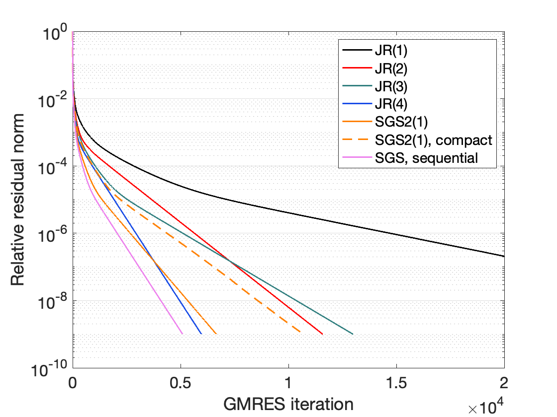
• SGS2(1, 1) performs a total of four SpMVs. According to the discussion in Section 5, SGS2(1,1) is likely to converge faster than JR(3), but it may converge slower than JR(4). The difference in the convergence rates was small, but JR(4) converged faster than SGS2(1, 1) in the first few iterations, but when more sweeps are performed, SGS2(1, 1) often converged faster than either JR(3) or JR(4) (as plotted in Figure 3).

• JR with the default damping parameter $\omega=1.0$ diverged, while SGS2 improved the convergence with additional inner sweeps. With a smaller damping factor $\omega=0.7$, both JR(4) and JR(3) converged faster.

• The figure displays the convergence rate of SGS2 in compact form. This requires fewer flops than the non-compact form, but may require extra inner sweeps to achieve the same rate of convergence. The plot confirms that the compact form achieves a smaller relative residual norm, but then stagnates after additional outer sweeps.

• A small number of inner sweeps ($n_{j}=1\sim 3$) were sufficient for SGS2 to match the convergence rate of the sequential SGS.

Figure 2: Convergence history of $\|\mathbf{b}-A\mathbf{x}_{k}\|_{2}/\|\mathbf{b}\|_{2}$ for SGS2. Elasticity problems.

Figure 3: Convergence history of $\|\mathbf{b}-A\mathbf{x}_{k}\|_{2}/\|\mathbf{b}\|_{2}$ for GS2 and JR. Laplace 2D problem. Number of SpMV. Ratio of SpMV flops versus SpMV flops using $A$.

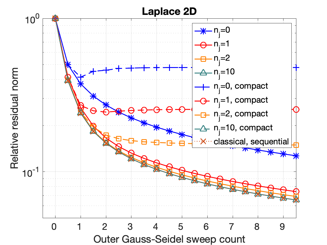
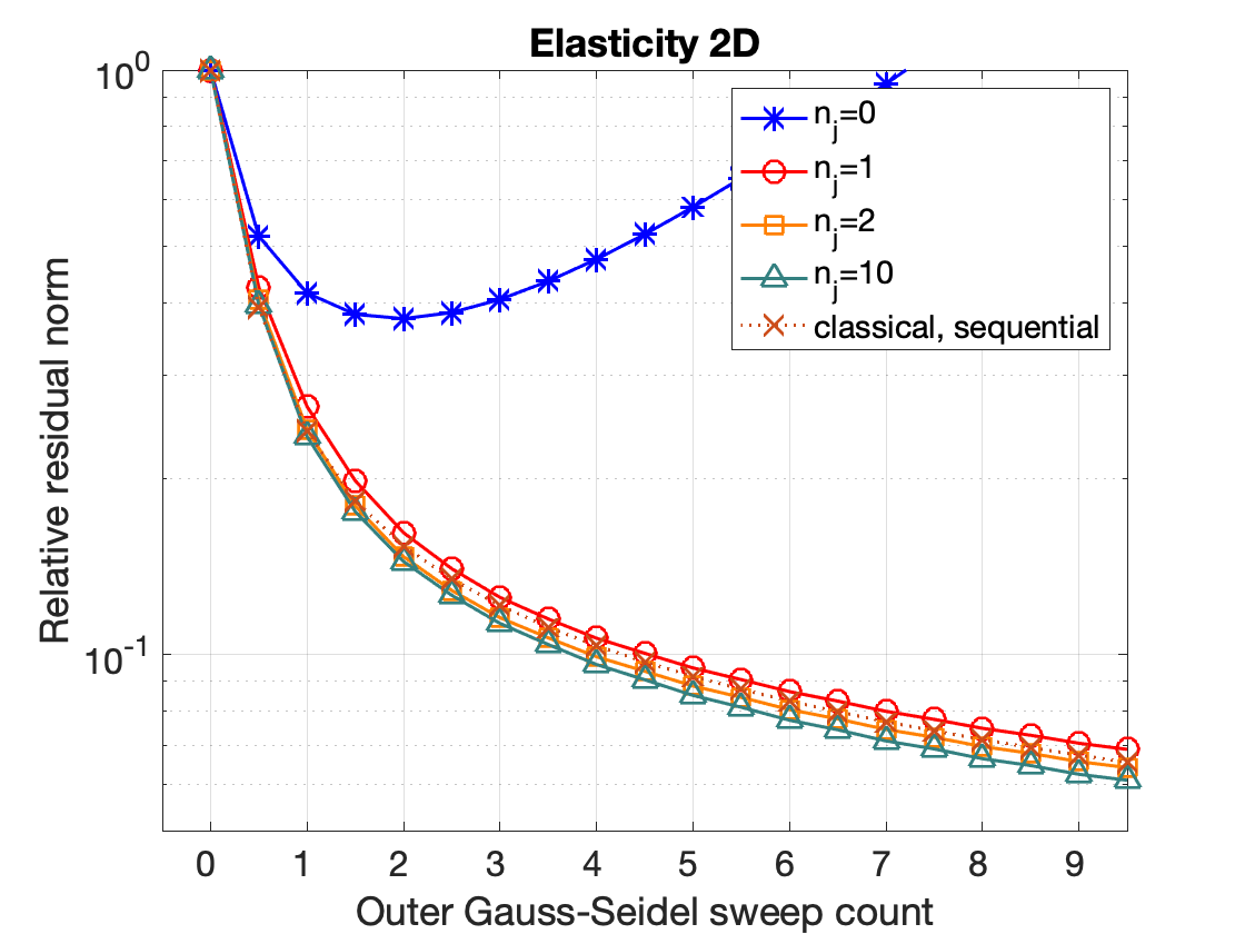
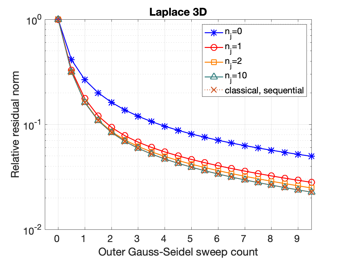
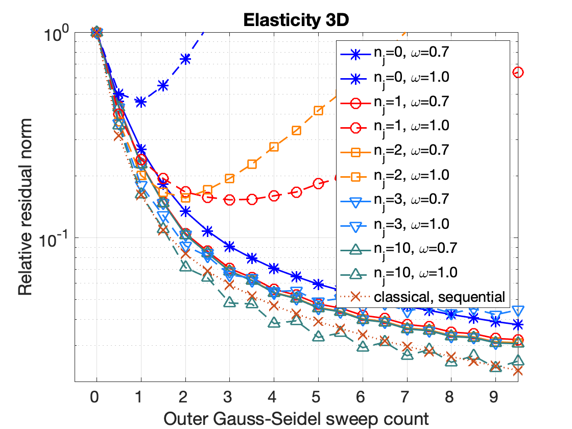
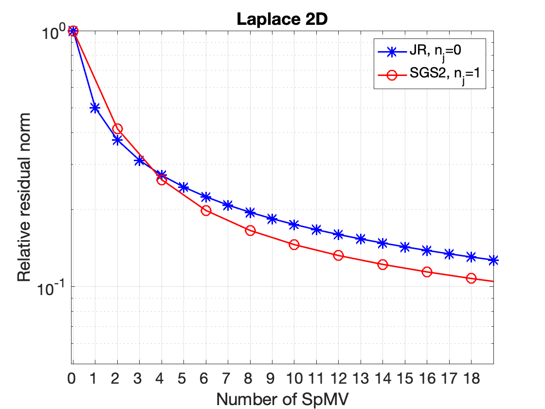
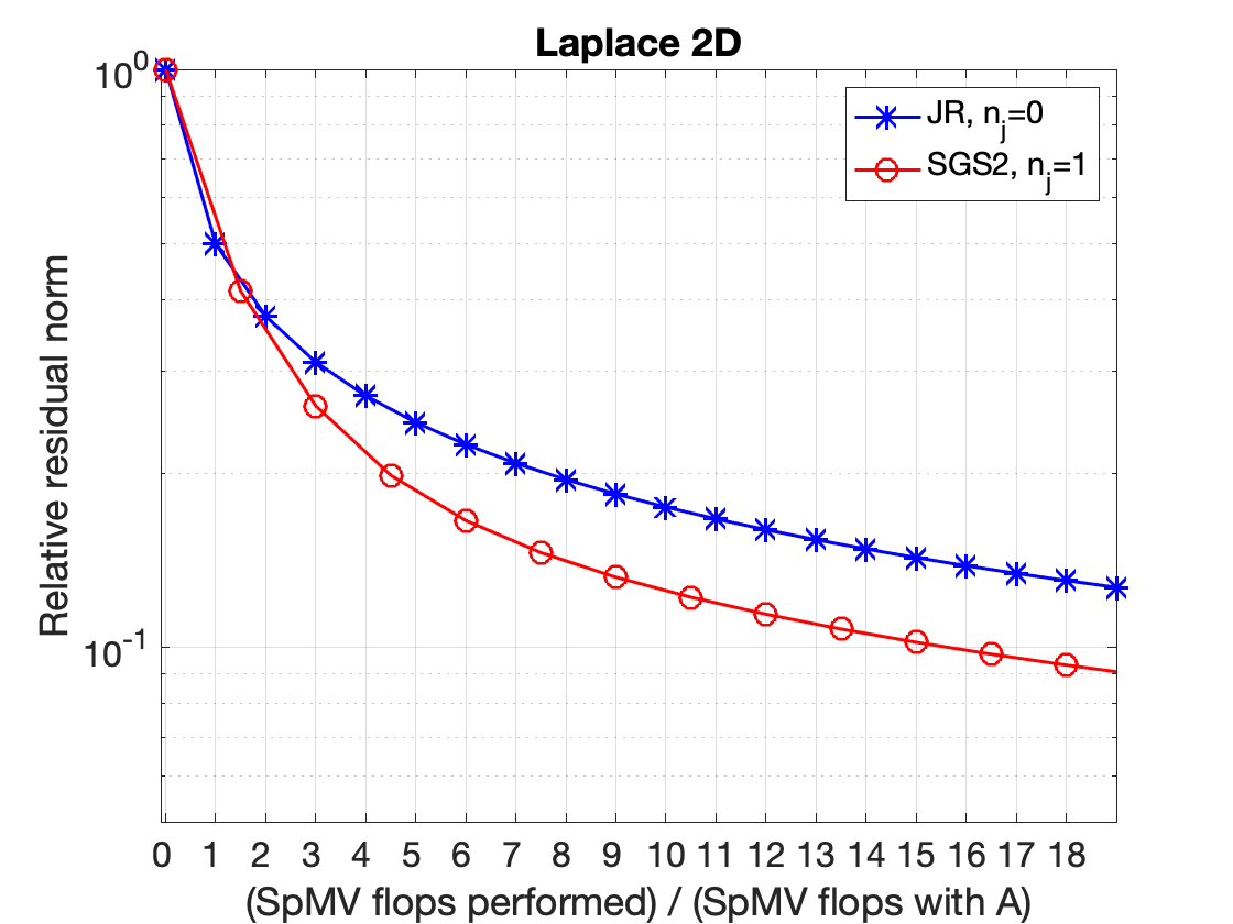
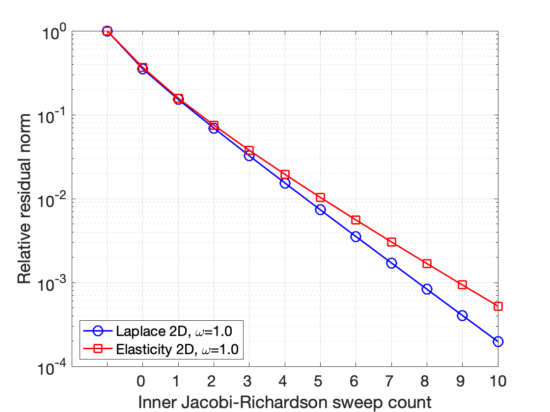
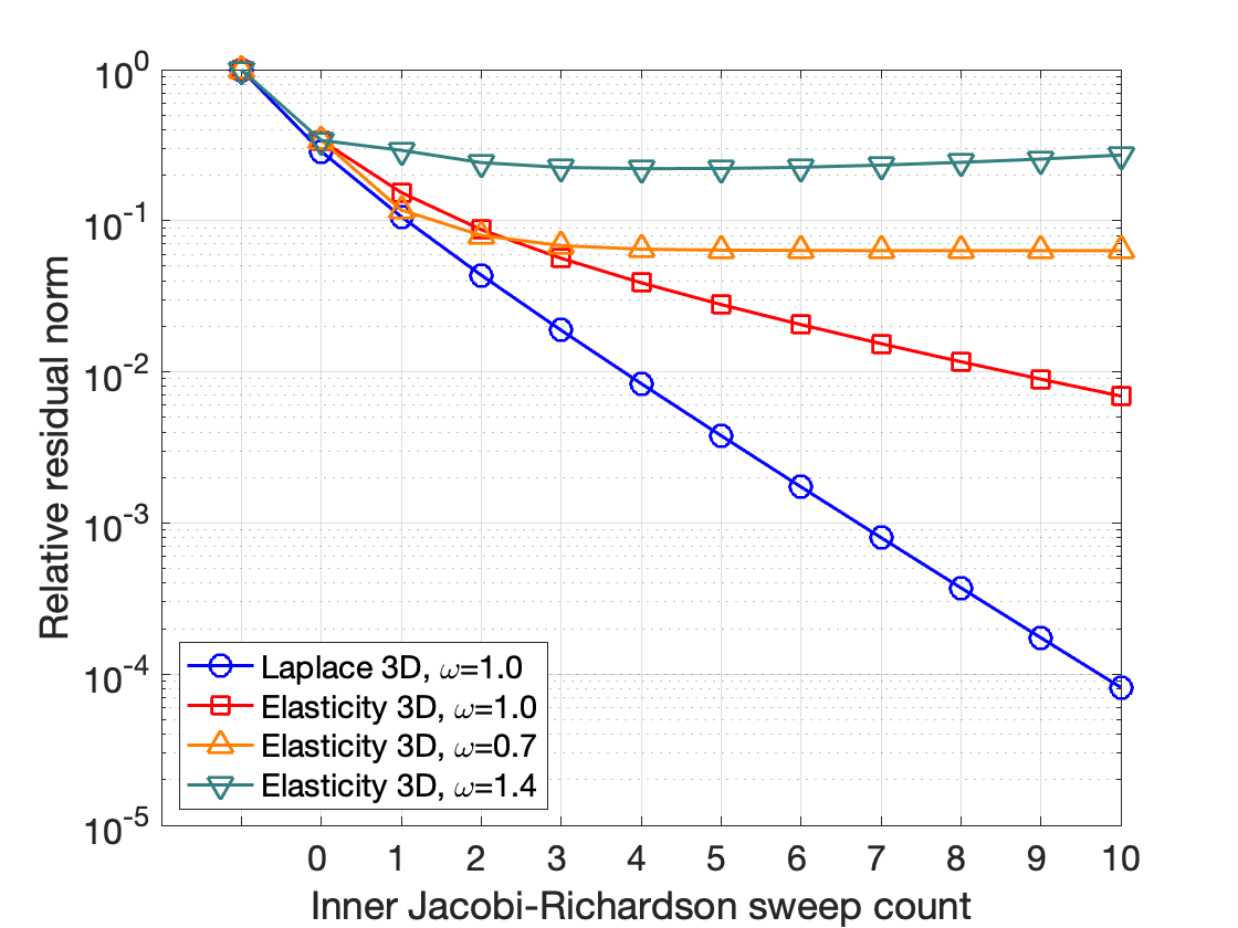
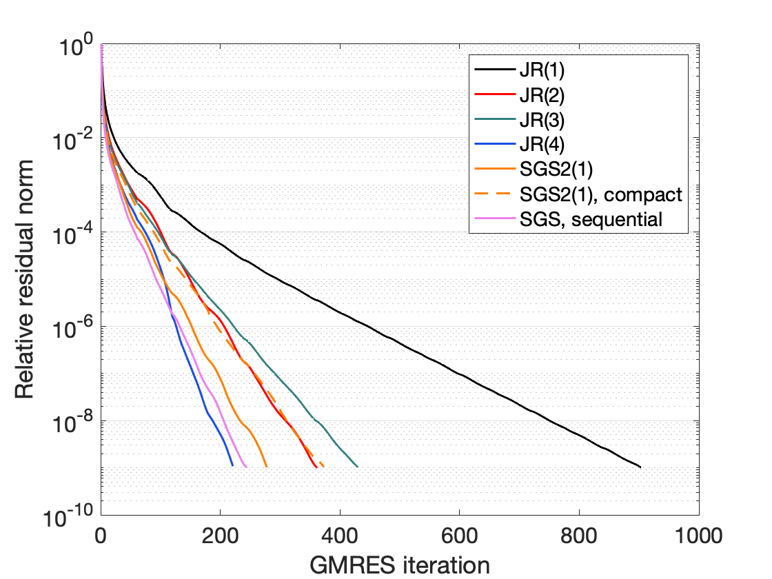
Figure 4 displays the inner JR convergence rate for solving the triangular system, while Figure 5 displays the convergence history with the SGS2 preconditioner. One to three JR sweeps were enough to reduce the relative residual norm by an order of magnitude, which is often enough to obtain the desired convergence rate. The iteration count is reduced by increasing the number of JR sweeps. The SGS2(1,1) iteration results in a faster convergence rate than JR(3) while it leads to a similar rate as JR(4), or sequential SGS(1). The latter degraded using the SGS2 preconditioner in compact form.

Figure 4: Convergence history of $\|\mathbf{r}_{l}-(L+D)\mathbf{g}_{j}\|_{2}/\|\mathbf{r}_{k}\|_{2}$, with inner JR sweeps $(n_{t}=5,n_{j}=2)$ for model problems. $n_{x}=20$.

(a) Laplace 2D ($n_{x}=1000$)

(b) Laplace 3D ($n_{x}=100$)

Figure 5: GMRES(60) convergence with Jacobi Richardson preconditioner.

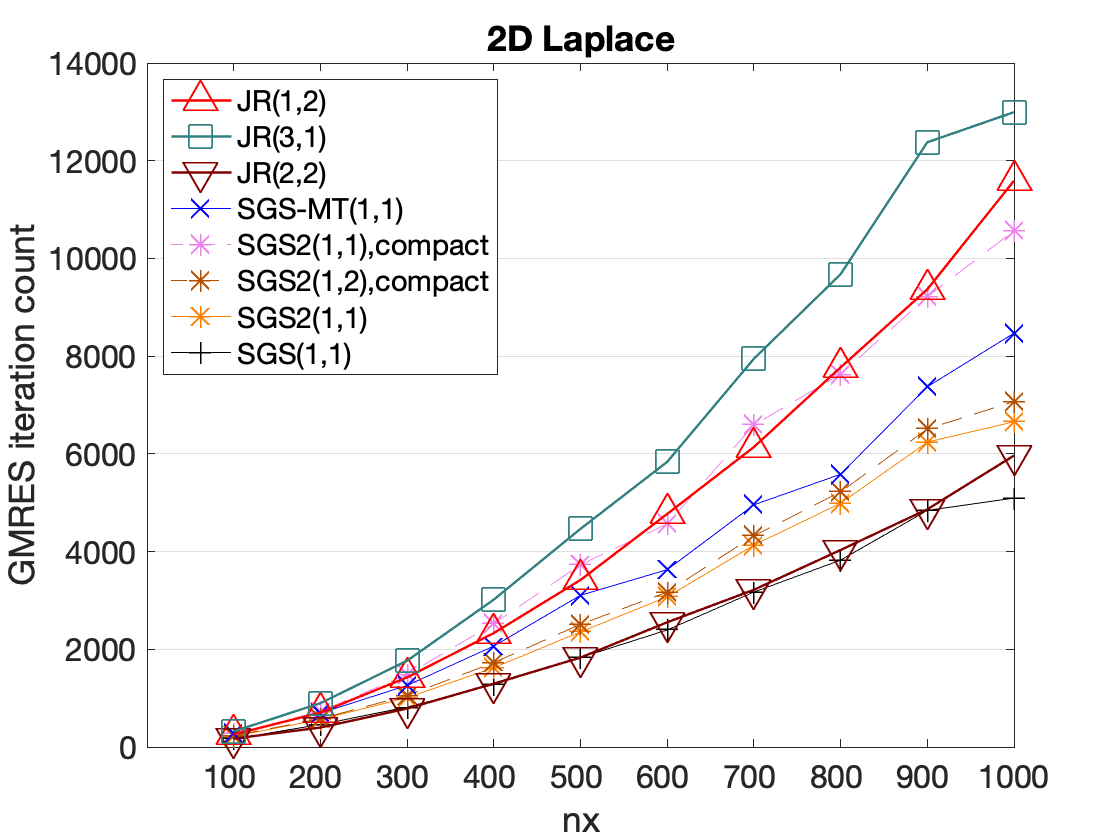
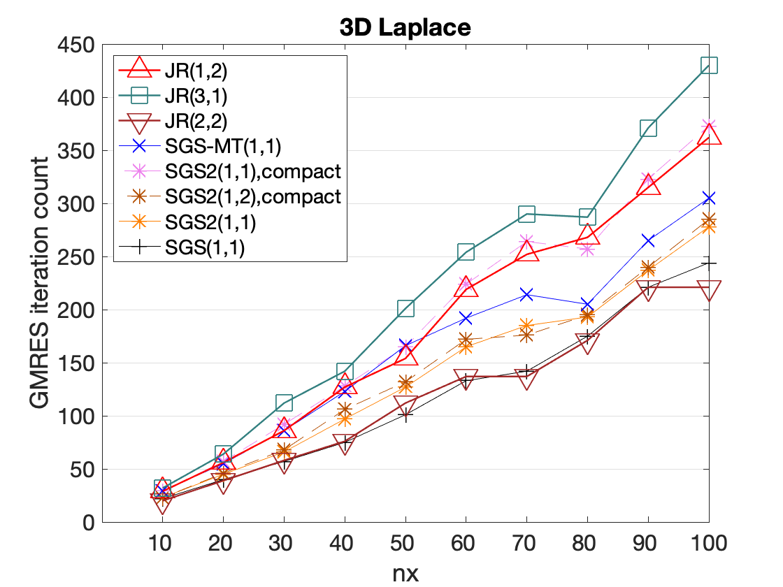
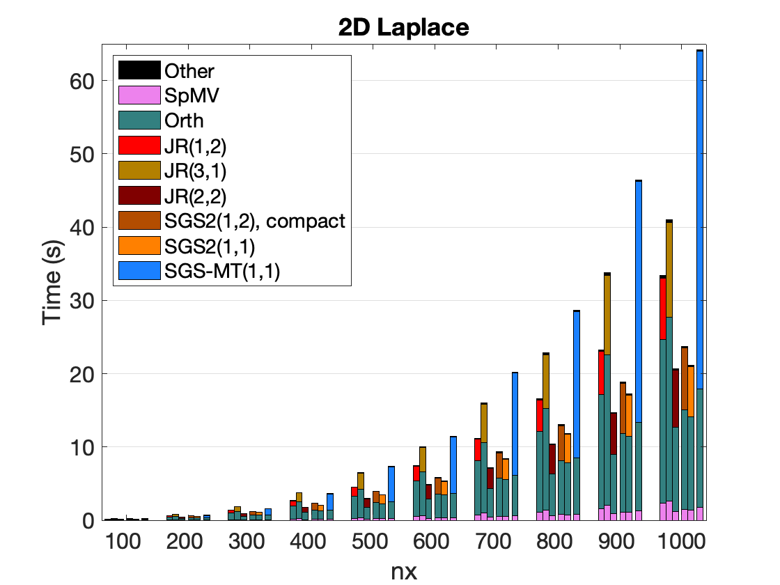
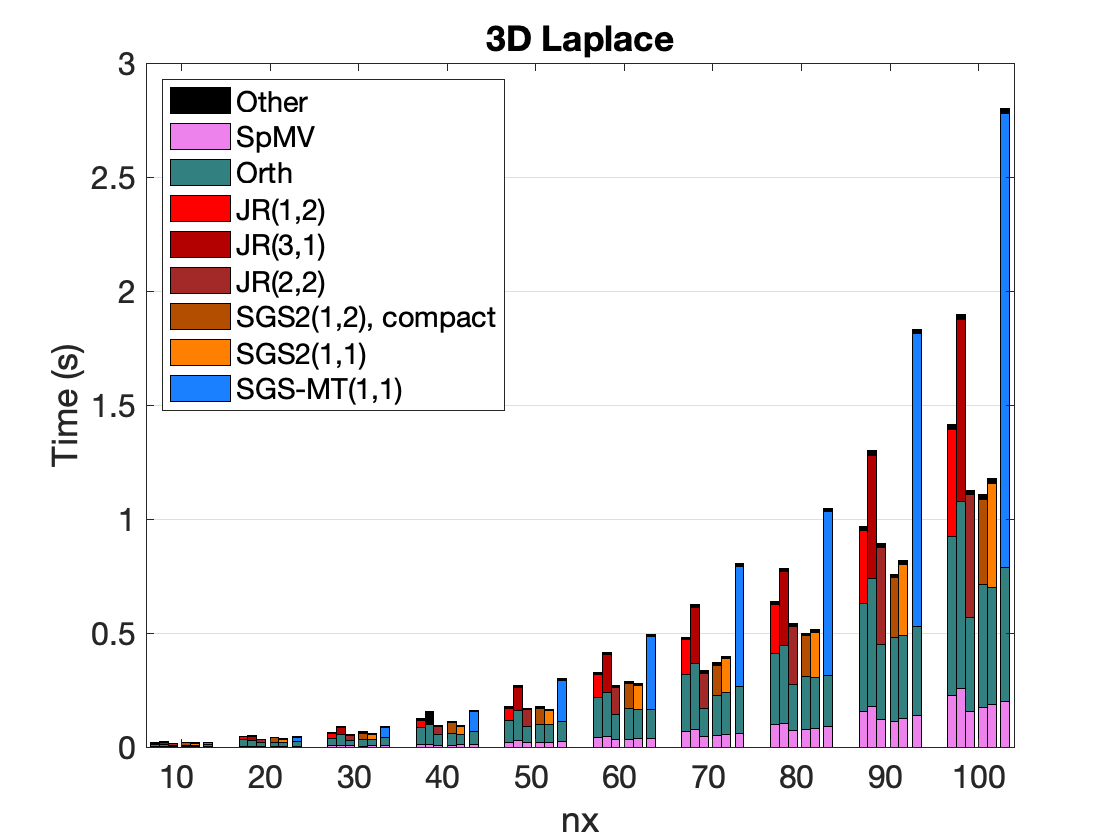
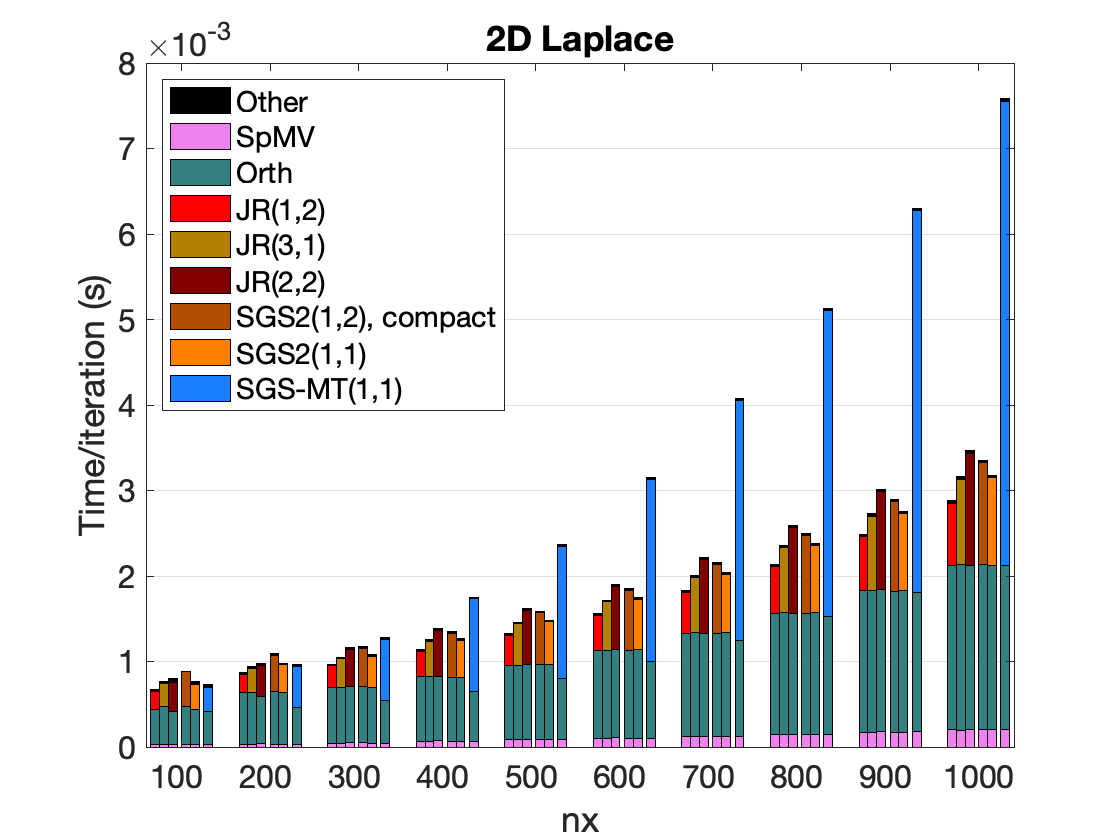
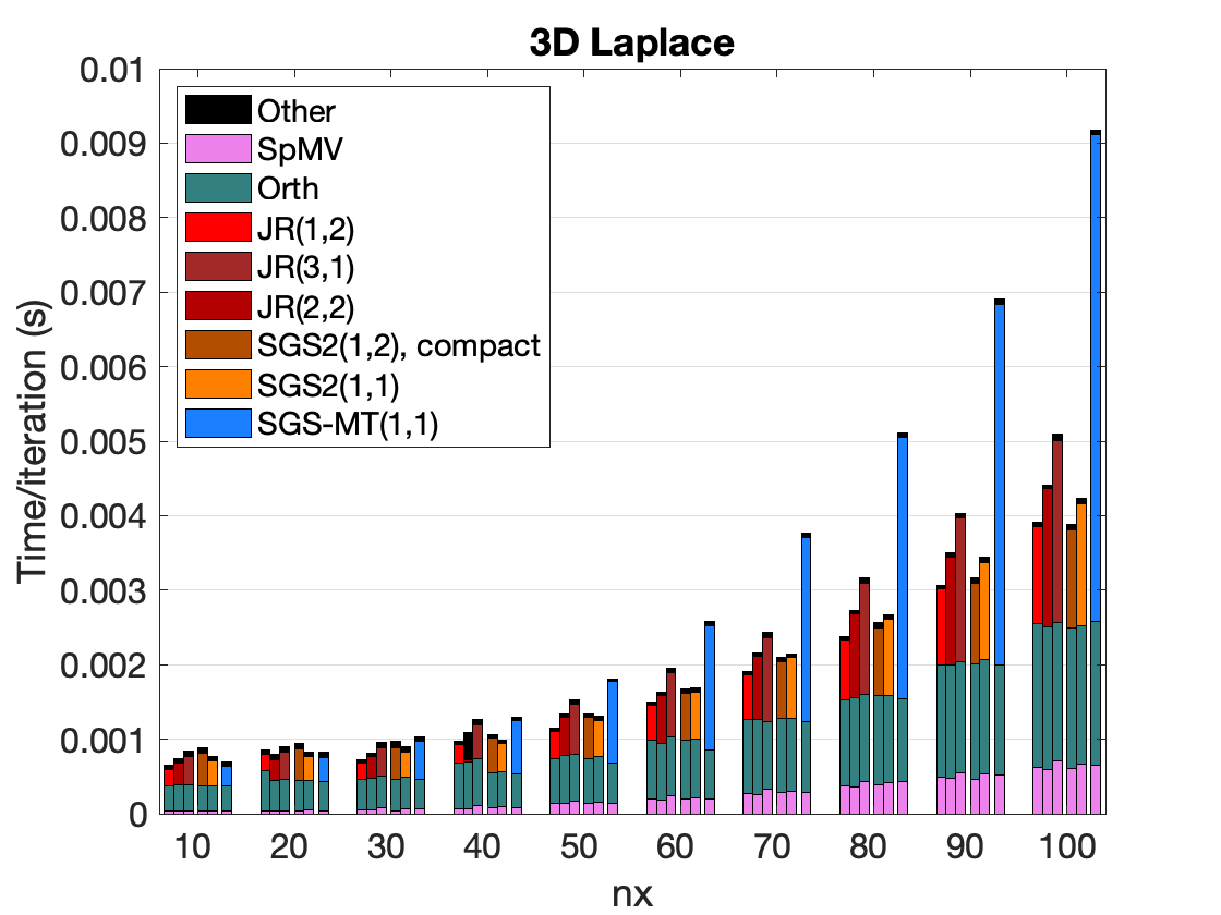
The time-to-solution with the SGS2 preconditioner was evaluated for model problems. Figures 6 through 8 compare the iteration count, time to solution, and time per iteration for the Laplace problems. Although a variable number of iterations is required to converge, the computed times of the different solvers were similar. To summarize,

• The solver converged with fewer iterations using SGS2(1,1) versus JR(3), but required more iterations than with JR(4), which achieved a convergence rate similar to the sequential SGS(1).

• In many cases, SGS2 requires more iterations than the sequential SGS, but fewer iterations than the MT-SGS, which could increase the iteration count.

• Compared with SGS2(1, 1), JR(4) exhibited a larger compute time per iteration but needed fewer iterations to converge. Overall, SGS2(1,1) and JR(4) obtained similar time to solution.

• Because SGS2 only needed a small number of SpMVs to obtain convergence rates similar to the sequential SGS, SGS2 was faster than sequential SGS or multi-threaded MT-SGS. Furthermore, an SpMV is inherently parallel, and thus SGS2 may also exhibit a slower increase in compute time with the problem size..

(a) Laplace 2D

(b) Laplace 3D

Figure 6: GMRES(60) iteration counts for Laplace problems.

(a) Laplace 2D

(b) Laplace 3D

Figure 7: GMRES(60) solution time on one GPU for Laplace problems.

(a) Laplace 2D

(b) Laplace 3D

Figure 8: GMRES(60) time per iteration on one GPU for Laplace problems.

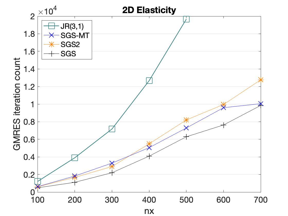
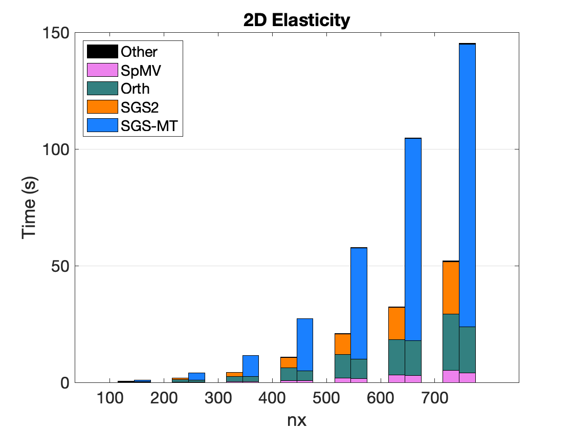
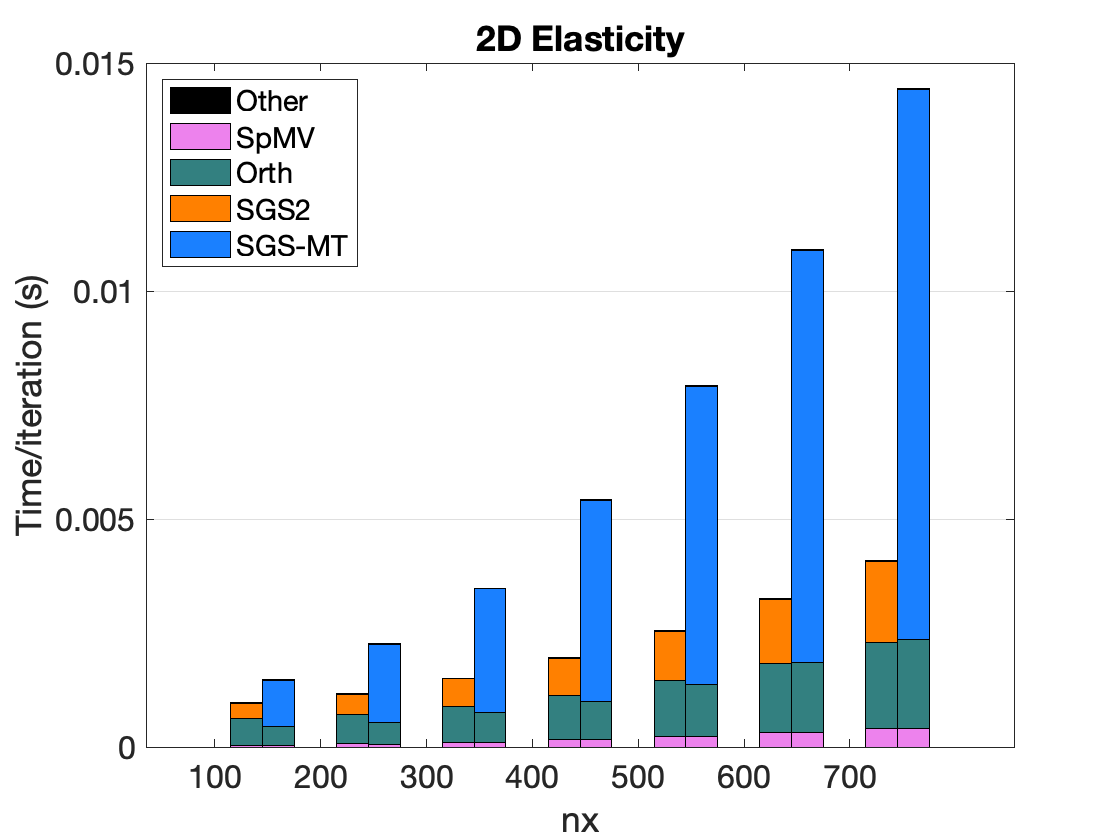
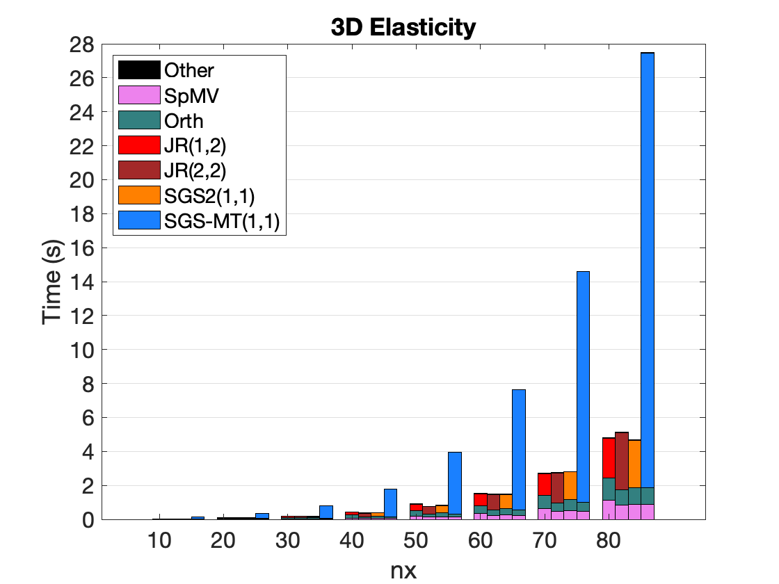
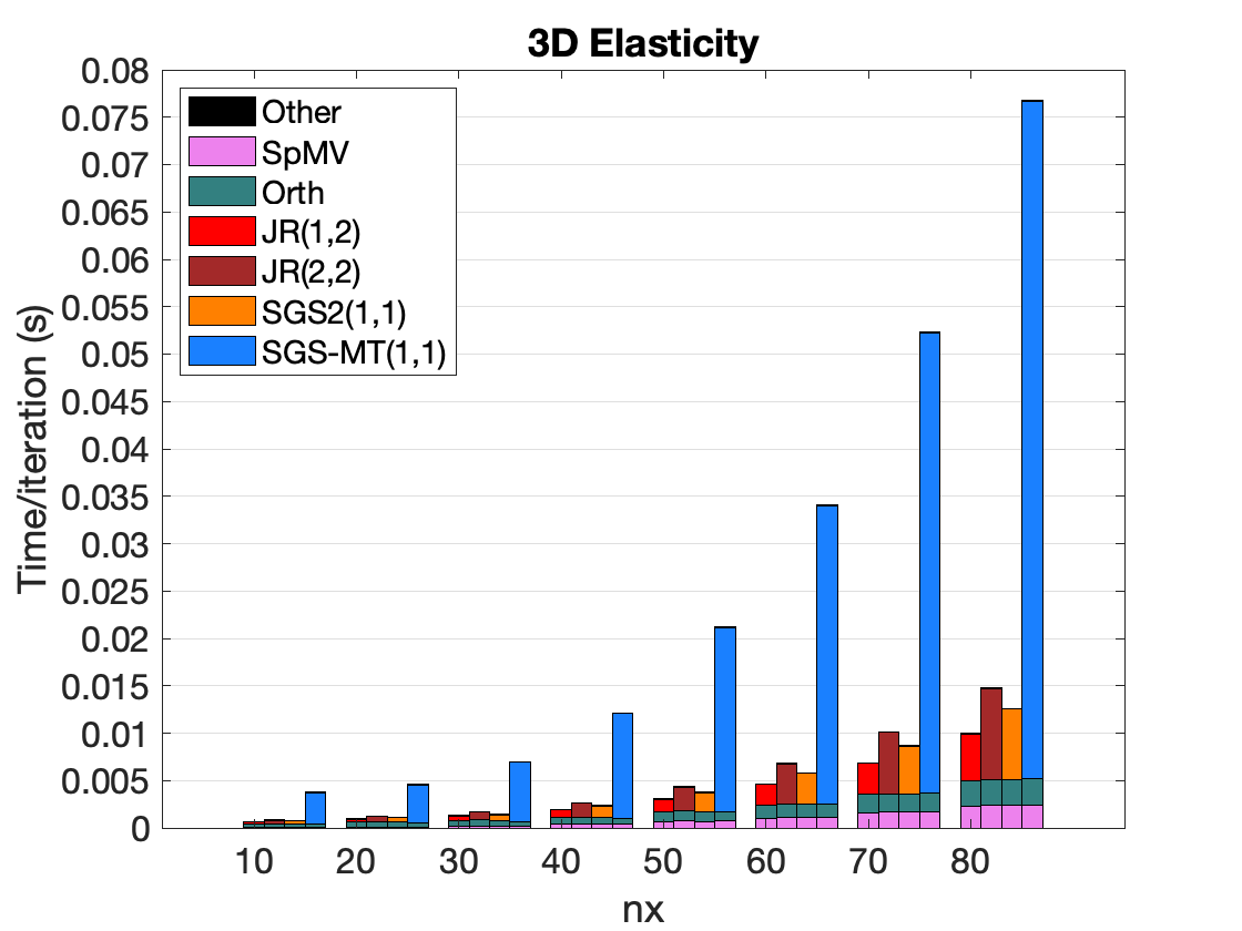
Figures 9a and 10 display iteration counts and compute times for the SGS2 preconditioner when applied to elasticity problems. The solver failed to converge using either JR(1,2) or JR(2,2), with the default damping factor of $\omega=1.0$. For the 3D problems, the damping factors were carefully selected to be (1.4, 1.2, 0.8, 0.7). To compare, the sequential SGS, MT-SGS, and SGS2 required about the same number of iterations, but SGS2 results in a much shorter time to solution.

(a) 2D problems.

(b) 3D problems.

Figure 9: GMRES iterations for elasticity problems.

(a) GMRES time to solution

(b) GMRES time per iteration

Figure 10: Compute times with one GPU for 2D elasticity problems.

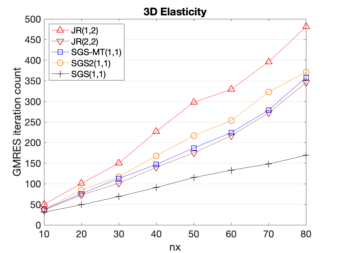
Next, the convergence rate with the SGS2 preconditioner applied to elasticity problems was studied, with $n_{x}=500$ and $n_{x}=20$. These were evaluated by varying the number of inner sweeps (i.e. $n_{j}$). SGS2 required a few inner sweeps to converge when a smaller damping factor is employed (see Figure 2). Figure 9b displays the iteration counts and Figure 12 provides the compute times for 3D elasticity problems.

Figure 11 displays the iteration counts with different values of the damping factor and a varying number of inner or outer sweeps for the SGS2 and JR, respectively. Only one outer sweep was performed for SGS, MT-SGS, and SGS2. In summary,

• With the default damping factor $\omega=1$, when SGS2 performs enough inner iterations, the same convergence rate is achieved as the sequential SGS.

• When $\omega=1$, JR diverges for this problem. As a result, even with multiple JR sweeps, the solver convergence was erratic.

• Conversely, JR converges well with a smaller damping factor $\omega=0.7$. Using a carefully-selected damping factor, the SGS2(1,1) iteration count was less than JR(3) but larger than JR(4).

• With increasing inner sweeps for SGS2, the iteration count is the same as sequential SGS.

$\omega$	1.6	1.5	1.4	1.3	1.2	1.1	1.0	0.9	0.8	0.7	0.6	0.5
SGS	52	49	49	51	53	56	61	68	78	87	93	102
SGS-MT	93	90	83	80	77	78	79	78	80	87	98	104
SGS2(1,1)	–	–	–	–	–	–	–	93	85	87	96	103
SGS2(1,2)	–	–	–	–	–	–	–	77	82	87	94	103
SGS2(1,3)	–	–	–	–	–	–	163	68	80	87	93	102
SGS2(1,4)	–	–	–	–	–	–	159	68	79	87	93	102
SGS2(1,5)	–	–	–	–	–	2650	62	68	79	87	93	102
SGS2(1,10)	–	–	–	–	–	92	61	68	78	87	93	102
JR(1)	213	213	213	213	213	213	213	213	213	213	213	213
JR(2)	–	–	–	–	–	–	–	–	–	101	108	119
JR(3)	457	399	341	265	233	211	194	152	122	107	100	101
JR(4)	–	–	–	–	–	–	–	–	–	73	76	82
JR(5)	1800	1332	957	696	488	347	227	155	104	78	73	75
JR(6)	–	–	–	–	–	–	–	–	–	56	60	67
JR(10)	–	–	–	–	–	–	–	–	–	43	46	51

Figure 11: GMRES iteration counts with one GPU for 3D elasticity problems, $n_{x}=20$. Outer and inner sweeps ($n_{t}$ and $n_{j}$ in Fig. 1).

(a) GMRES solution time and time per iteration

Figure 12: Solution time with one GPU for 3D elasticity problems.

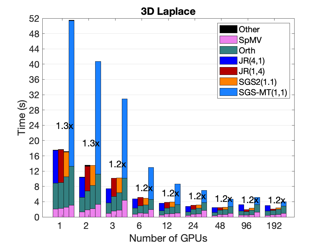
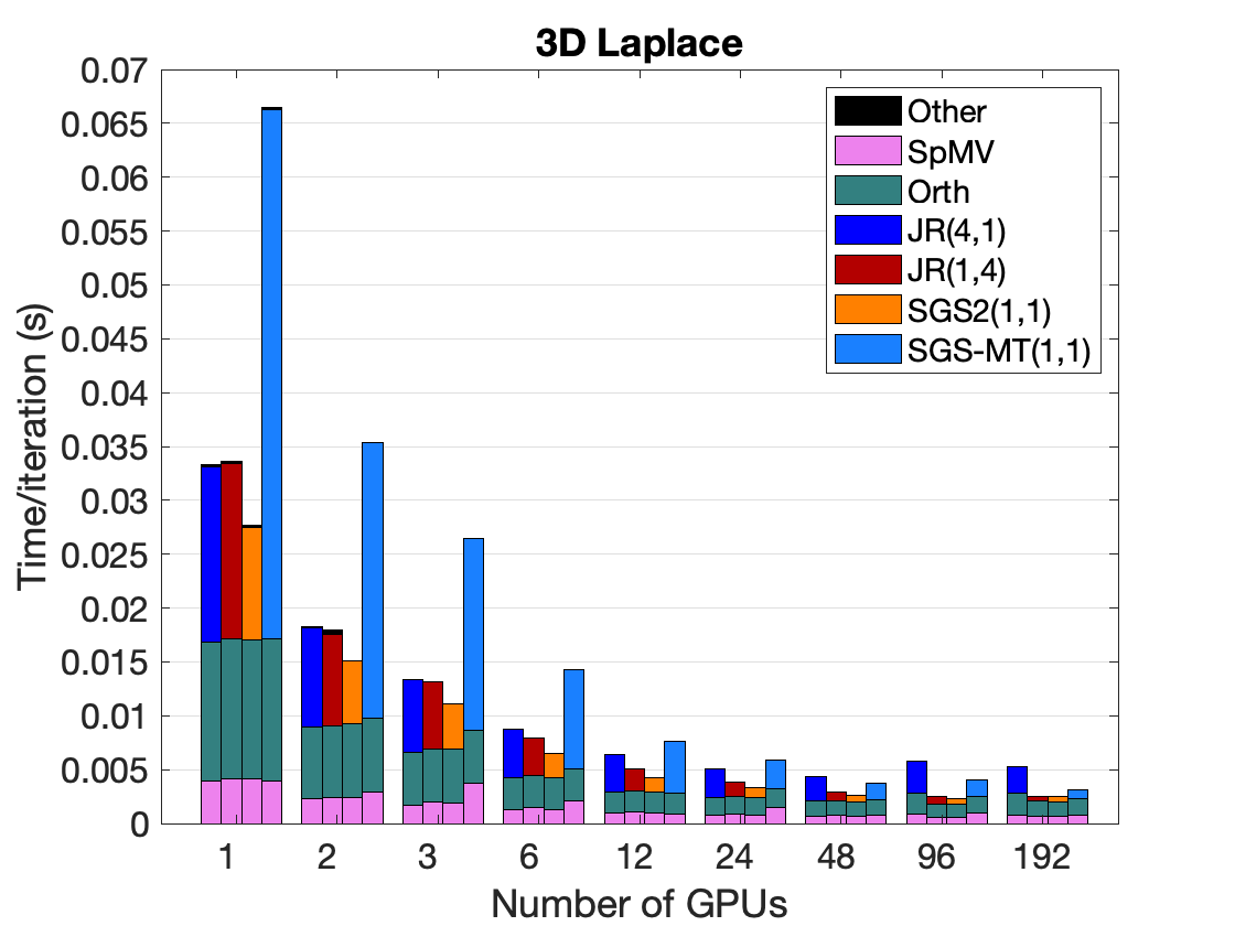
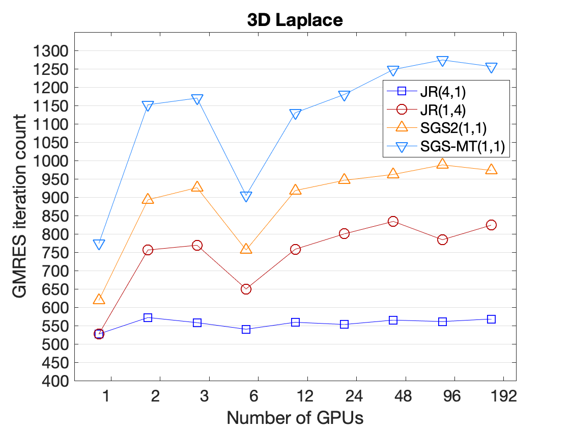
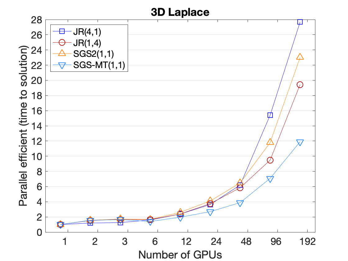
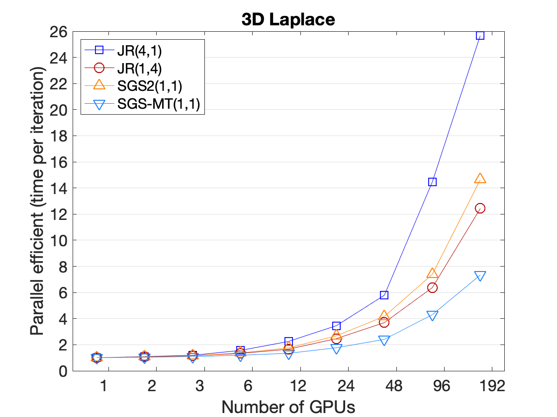
Finally, Figure 13 displays the parallel strong-scaling when solving the Laplace 3D problem. JR(4,1) and JR(1,4) are the “global” and “local” JR preconditioners that apply the JR iteration on the global and local matrix, respectively. The iteration count remains constant when using JR(4,1), but may grow with the number of GPUs using JR(1,4) (see Figure 14). Thus, JR(4,1) performs well on a small number of GPUs (due to the faster solver convergence rate), but JR(1,4) performs better on a larger number of GPUs (due to reduced communication cost).

Figure 13: GMRES(60) strong scaling for Laplace 3D problems with $n_{x}=200$.

Figure 14: GMRES(60) parallel efficiency for Laplace 3D problems.

9 Experimental Results with Suite Sparse Matrices

Matrices from the Suite-Sparse matrix collection are now used to study the performance of the Trilinos SGS2 preconditioner. For these experiments, symmetric positive definite (SPD) matrices are the focus and the conjugate gradient algorithm is applied (CG) [26] as our Krylov solver. Figure 15 lists the test matrices, and Figure 16 displays the performance. When SGS2 requires just one inner sweep to obtain the same convergence rate as that of the classical SGS, it can reduce the time to solution. Also, SGS2 often outperformed JR(4), even though it may require more iterations (because it was cheaper to apply).

For eight of the test matrices, with the default damping factor, JR diverged when using either the coefficient matrix or the triangular part of the matrix. Consequently, the solver did not converge using either JR(4) or SGS2(1,1) for these matrices. Figure 17 displays the performance with SGS2(1,1) using a different damping factors $\gamma$ for the inner JR sweeps. The default damping factor was set for the outer sweep (i.e., $\omega=1.0$), as in Figure 16. The robustness of the inner JR sweep, and thus the convergence rate of SGS2 and GMRES, is improved using a smaller damping $\gamma$.

CFD Structural Problem Thermal Problem EM id 1 2 3 4 5 6 7 8 9 10 11 12 13 name PPoiss cfd1 cfd2 para_fem bcsstk17 af_shell7 Fault639 Emil923 Hook1498 ted_B therm1 therm2 tmt_sym $n$ 14,822 70,656 123,440 525,825 10,974 504,855 638,802 923,136 1,498,023 10,605 82,654 1,228,045 726,713 $\frac{nnz}{n}$ 48.3 25.8 25.0 7.0 39.1 34.8 42.7 43.7 39.6 13.6 6.9 7.0 7.0

Figure 15: Test matrices (SPD) from Suite-Sparse matrix collection. Solution time (seconds). Rows $n$. Non-zeros per row $nnz(A)/n$.

SGS SGS-MT SGS2(1,1) JR(4) JR(1) 1 1.59 ( 0.97, 243) 0.78 ( 0.70, 269) $--$ $--$ $--$ 2 8.30 ( 4.99, 486) 1.57 ( 1.33, 648) $--$ $--$ $--$ 3 54.25 (33.29, 1,945) 8.04 ( 6.96, 2,577) $--$ $--$ $--$ 4 57.69 (37.35, 1,434) 6.39 ( 5.34, 1,465) 2.71 ( 1.69, 1,448) 4.18 ( 3.43, 1,050) 3.25 (1.78, 2,099) 5 4.93 ( 2.90, 1,122) 3.64 ( 3.25, 1,160) $--$ $--$ $--$ 6 212.20 (130.70, 1,400) 17.83 (16.61, 1,407) $--$ $--$ $--$ 7 831.30 (528.40, 3,339) 56.48 (53.76, 2,839) $--$ $--$ $--$ 8 1089.0 (683.30, 3,029) 100.6 (96.05, 3,680) $--$ $--$ $--$ 9 989.5 (652.40, 1,785) 81.66 (78.13, 1,972) $--$ $--$ $--$ 10 0.033 (0.015, 11) 0.026 (0.021, 14) 0.015 (0.006, 16) 0.329 (0.249, 329) 0.269 (0.147, 505) 11 5.54 (3.2, 701) 0.87 (0.61, 726) 0.55 (0.34, 718) 0.541 (0.385, 408) 0.524 (0.213, 821) 12 278.50 (196.50, 2,657) 24.54 (21.81, 2,731) 7.67 (4.98, 2,714) 9.27 (7.75, 1,541) 7.05 (4.01, 3,090) 13 105.60 (69.67, 1,857) 13.30 (11.44, 2,363) 4.41 (2.74, 2,139) 23.22 (19.18, 5,235) 16.63 (9.18, 9,632)

Figure 16: Solution time in seconds with Suite-Sparse matrices. The numbers in parentheses are time to apply the preconditioners and CG iteration counts.

Matrix ID $\gamma$ 1 2 3 5 6 7 8 9 12 0.1 0.47 (626) 1.47 (1,627) 7.09 (6,606) 1.71 (2,342) 7.59 (3,147) 21.13 (6,485) 39.09 (8,833) 30.64 (4,708) 10.24 (4,822) 0.2 0.38 (503) 1.11 (1,221) 5.13 (4,823) 1.30 (1,782) 6.91 (2,845) 17.52 (5,376) 32.50 (7,351) 26.42 (4,069) 9.27 (4,347) 0.3 0.31 (415) 0.91 (998) 16.51 (15,535) 1.07 (1,474) 5.89 (2,429) 14.83 (4,555) 27.31 (6,181) 22.93 (3,529) 8.38 (3,921) 0.4 0.27 (359) 10.49 (11,633) $--$ ($--$) 3.39 (4,657) 5.14 (2,120) 12.65 (3,878) 23.64 (5,346) 20.07 (3,085) 7.58 (3,544) 0.5 0.33 (456) $--$ ($--$) $--$ ($--$) $--$ ($--$) 4.59 (1,894) 11.38 (3,491) 21.12 (4,769) 17.93 (2,755) 6.84 (3,210)

Figure 17: CG iteration counts with SGS2(1,1) preconditioner. The number in parentheses displays the CG iteration count.

10 Experimental Results using Lower Precision Preconditioner

Figure 18: Outer SGS2(1,1) and Inner JR convergence for 2D Laplace ($n_{x}=1000$).

	SGS, double	SGS, single	SGS2, double	SGS2, single	MT, double,	MT, single
# of GMRES iters	5,095	5,095	6,656	6,656	8,236	7,745
time to apply SGS	201.9	178.1	8.13	5.63	28.28	25.99
time to solution	315.7	205.5	23.21	21.33	46.68	43.99

(a) GMRES(60).

	SGS, double	SGS, single	SGS2, double	SGS2, single	MT, double,	MT, single
# of CG iters	1,108	1,108	1,279	1,279	1,627	1,911
time to apply SGS	43.07	38.01	1.54	1.07	5.48	6.28
time to solution	65.35	41.94	2.49	2.13	6.71	7.77

(b) CG.

Figure 19: Compute time (seconds) of CG with 2D Laplace $(n_{x}=1000)$ using SGS preconditioner in double or single precision.

In experiments with the GS2 preconditioner, only one outer and inner sweep were enough to obtain a convergence rate similar to that with the classical GS preconditioner. Hence, high-accuracy is not needed from the outer GS iterations or from the inner JR iterations. To improve the performance, the use of lower-precision floating point arithmetic was investigated for the preconditioner. Our main concern is to determine if the quality of the preconditioner would degrade in lower precision. This depends on the properties of the matrix that affect the behavior of GS in finite precision, such as its maximum attainable accuracy and convergence rate. For example, GS is norm-wise backward stable and its attainable relative residual norm is upper-bounded by $\epsilon\kappa(A)$ [27], while each GS or JR sweep would reduce the relative residual norm by a factor of at least $\|I-M^{-1}A\|$. Using single precision for GS, the quality of the preconditioner should be maintained (same as GS in double precision) if one sweep of GS in double precision does not reduce the residual norm below the attainable accuracy of GS in single precision (e.g. $\kappa(A)<\mathcal{O}(1/\epsilon_{s})$ and $\mathcal{O}(\epsilon_{s})\kappa(A)<\|I-M^{-1}A\|$, where $\epsilon_{s}$ is the machine precision in single precision).

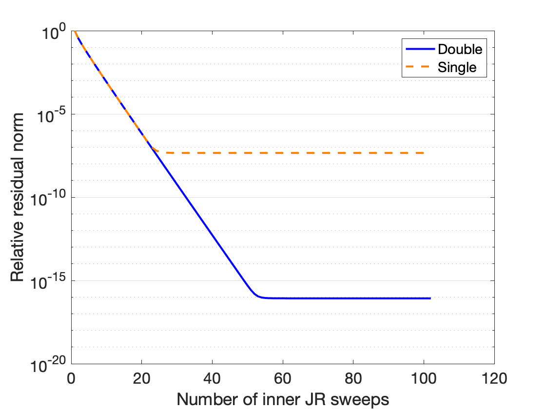
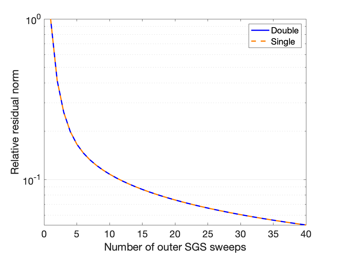
Figure 18 indicates that the outer GS and inner JR iteration in single precision converge in the same way as in double precision until the iteration achieves the maximum solution accuracy and begins to stagnate. Figures 19 and 20 then display the performance of CG using the SGS preconditioner in double or single precision. The CG convergence rate was maintained using the single-precision preconditioner for these test matrices, while the time for applying the preconditioner was reduced by factors of around $1.4\times$.

	4 ($\gamma=1.0$)			6 ($\gamma=0.5$)			7 ($\gamma=0.5$)			12 ($\gamma=1.0$)
	double	single	speedup	double	single	speedup	double	single	speedup
# of CG iters	1,448	1,448	–	1,894	1,894	–	3,491	3,532	–	2,714	2,714	–
time to apply SGS	1.69	1.14	1.48	3.30	2.33	1.41	8.01	5.99	1.35	4.98	3.55	1.40
time to solution	2.71	2.34	1.16	4.59	3.86	1.18	11.38	9.75	1.17	7.67	6.89	1.11

Figure 20: Compute time (seconds) CG with the Suite Sparse matrices in Figure 15 using SGS2 preconditioner in double or single precision.

11 Experimental Results with Nalu-Wind

To study the performance of the two-stage Gauss-Seidel preconditioner and smoother in a practical setting, incompressible fluid flow simulations were performed with Nalu-Wind [5]. This is the primary fluid mechanics code for the ExaWind project, one of the application projects chosen for the DOE Exascale Computing Project (ECP) and is used for high-fidelity simulations of air flow dynamics around wind turbines. Nalu-Wind solves the acoustically incompressible Navier-Stokes equations, where mass continuity is maintained by an approximate pressure projection scheme. The governing physics equations for momentum, pressure, and scalar quantities are discretized in time with a second-order BDF-2 integrator, where an outer Picard fixed-point iteration is employed to reduce the nonlinear system residual at each time step. Within each time step, the Nalu-Wind simulation time is often dominated by the time required to setup and solve the linearized governing equations, using either hypre or Trilinos solver package. To solve the momentum equations, Nalu-Wind typically employs Gauss-Seidel (GS) or symmetric Gauss-Seidel (SGS) iteration as a preconditioner to accelerate the GMRES convergence. The pressure systems are solved using GMRES with an algebraic multigrid (AMG) preconditioner, where a Gauss-Seidel or Chebyshev polynomial smoother is applied to relax or remove high energy components of the solution error (e.g. those associated with the large eigenvalues of the system), which the coarse-grid solver fails to eliminate.

To study the performance of GS2, representative incompressible Navier-Stokes wind-turbine simulations were performed (an atmospheric boundary layer (ABL) precursor simulation on a structured mesh). The strong scaling performance of both the Trilinos and hypre solver stacks were evaluated. We note that it is possible to generate segregated linear equations for solving the momentum problems. This reduces the sizes of the linear systems, and also reduces the number of nonzero entries per row. This technique can reduce the time to solutions, especially when the underlying computation kernels are optimized to take advantage of the multiple right-hand-sides. In the following, this option was not used for the experiments using Trilinos, while this option was employed for the experiments using hypre.

11.1 Experimental Results with Trilinos

(a) For an SGS sweep of the momentum solves.

(b) For an SGS sweep of the continuity solve.

Figure 21: Convergence history of the relative residual norm, $\|\mathbf{r}_{l}-(L+D)\mathbf{g}_{k}^{(j)}\|_{2}/\|\mathbf{r}_{k}\|_{2}$, with inner Jacobi-Richardson sweeps for the ABL 40m simulation.

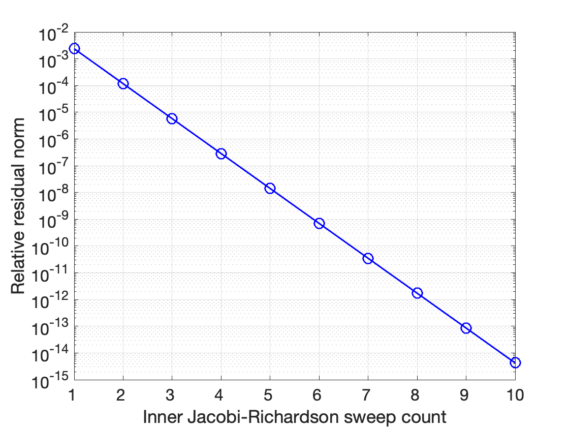
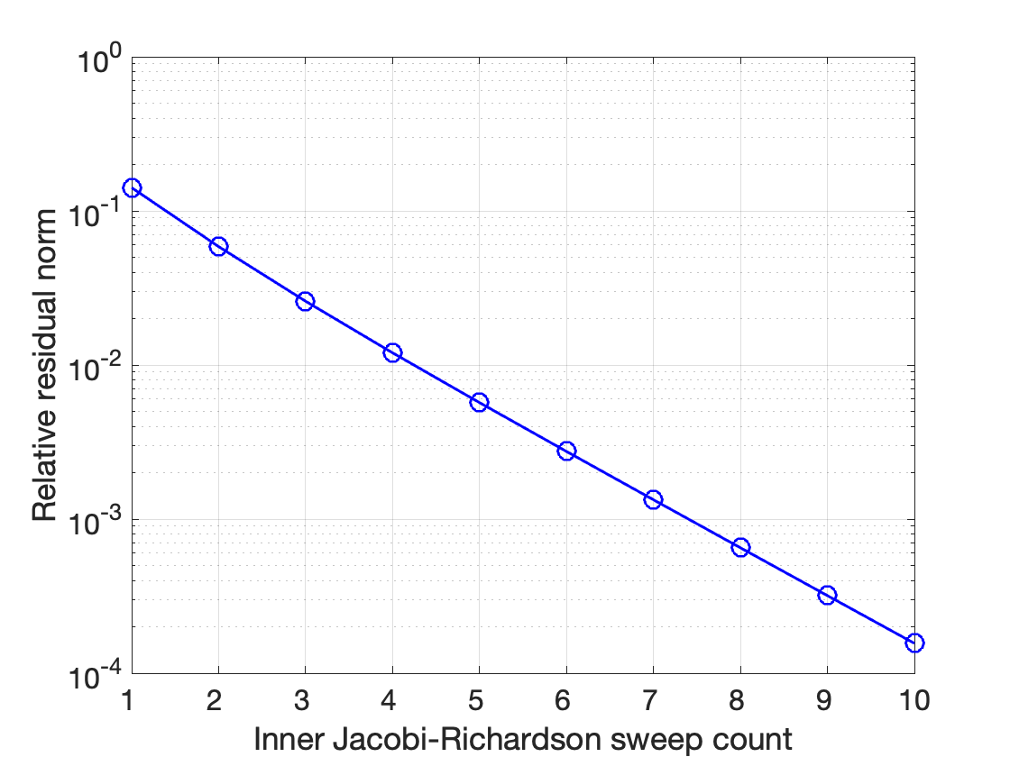
Figure 21 displays the convergence history of the inner sweep for one time-step of the Nalu-Wind ABL precursor simulation on a 40m resolution mesh. In this simulation, the solver converged with the same number of iterations to a relative residual tolerance level of $1\times 10^{-6}$ using just one sweep of the inner Jacobi iteration for SGS2 as that using the sequential SGS preconditioner. Moreover, Figure 22 reports the iteration counts for ten time-steps of the Nalu-Wind ABL precursor 40m simulation, where the compact form leads to a significantly larger number of iterations for the pressure systems. On another note, the compact form worked well as the preconditioner for the remaining problems (with an extra inner sweep for the compact form, the solver often converged similar to with the non-compact form). A comparison of these is presented in Section 5 along with similar results for model problems in Section 8.

				two-stage
	No	Seq	MT	non-compact		compact
Inner sweep	–	–	–	0	1	1	2	4	6
Continuity	–	285	311	511	300	2410	863	401	314
Enthalpy	419	81	121	122	84	84	82	81	81
Momentum	270	83	108	81	83	90	83	83	83
TKE	334	80	120	104	81	81	80	80	80

Figure 22: Solver iteration counts with ten time-step ABL 40m simulation on one GPU with SGS preconditioner for momentum and turbulent kinetic energy (TKE) systems (one SGS sweep) and continuity (three SGS sweeps).

Next, consider the performance of Trilinos solvers for the Nalu-Wind simulation using the ABL precursor 20m mesh. To solve the continuity system, Trilinos uses a smoothed aggregation SA-AMG preconditioner and a Chebyshev smoother. The three remaining equations (Momentum, TKE and Enthalpy) are solved with a GS preconditioner. In this section, GS2 is applied as alternative to the sequential GS preconditioner.

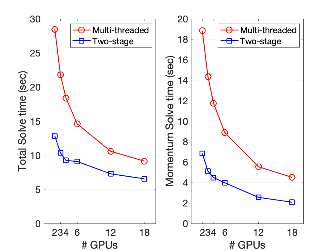
Figure 23a displays the strong scaling of the Trilinos solvers for the Nalu-Wind simulation using the ABL precursor mesh. The maximum number of iterations required to solve these linear systems was low but remains constant across all mesh resolutions tested. Even though the same Chebyshev smoother was used for solving the pressure system, compared to using the classical SGS preconditioner, the total solve time was still reduced using SGS2 preconditioner for the remaining systems. The performance advantage of using the SGS2 preconditioner over the multi-threaded SGS was maintained over multiple nodes.

(a) Strong scaling Trilinos.

(b) Strong scaling hypre.

Figure 23: Parallel scalability of solve time on Summit for ABL 20m precursor.

11.2 Experimental Results with hypre

Strong scaling studies for the hypre solver stack have also been performed for the ABL precursor Nalu-Wind simulation. The GS2 iteration was implemented as both the momentum equation preconditioner and as a smoother for the GMRES solver with classical Ruge-Stüben C-AMG preconditioner for the pressure continuity solver [28]. For the C-AMG set-up, HMIS coarsening is specified for the ABL precursor problem. One sweep of the GS2 smoother is applied at each level of the C-AMG $V$-cycle. The strength of connection threshold is $\theta=0.25$ and two levels of aggressive coarsening reduce the preconditioner cost and coarse-grid operator complexity.

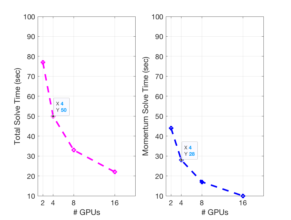
MGS-GMRES solver compute times are reported for ten time-step integrations from a restart of the Nalu-Wind model  [29, 30] . Momentum solve time exhibits nearly perfect strong scaling, every time the number of ranks is doubled, the compute time is halved (Figure 23b, right panel). The continuity solver time exhibits sub-linear strong scaling. This may also be attributed to additional computation and communication overheads in the C-AMG $V$-cycle such as the MPI communication associated with the prolongation and restriction matrix-vector products. The authors are currently investigating the source of these sub-linear scaling solver times.

12 Conclusion

A two-stage iterative variant of the Gauss-Seidel relaxation was examined as an alternative to the sequential GS algorithm based on a sparse triangular solver. The two-stage approach replaces the triangular solve with a fixed number of inner relaxation sweeps, and is much more amenable to an efficient parallel implementation on many-core architectures. When a small number of inner sweeps is needed, the two-stage variant often outperforms the sequential approach.

To study the performance of the GS2 algorithm as a preconditioner and smoother in a practical setting, the algorithm was employed in Nalu-Wind incompressible fluid flow simulations [5]. GS2 was applied to accelerate convergence for the momentum equation and as a smoother for the AMG preconditioner when for the pressure solver. Our performance results demonstrate that the GS2 preconditioner requires just one inner sweep to obtain a GMRES convergence rate similar to the sequential algorithm, and thus it achieves a faster time to solution, both on CPU and GPU. Another advantage, not discussed earlier, is that the set-up cost for GS2 is minimal and does not require eigenvalue estimates. The setup cost influences the choice of preconditioner, because the setup is performed at each time step due to mesh movement. In addition, to obtain the desired convergence rate of SGS2 and GMRES, the required parameters (e.g., number of inner sweeps and damping factors) depend on the properties of the coefficient matrices. The relationship between the inner stopping criteria and the outer convergence rate is being examined in order to determine the appropriate stopping criteria.

References

- [1] Y. Saad, M. Schultz, GMRES: A generalized minimal residual algorithm for solving nonsymmetric linear systems, SIAM J. Sci. Comput. 7 (1986) 856–869.
- [2] M. Heroux, R. Bartlett, V. Howle, R. Hoekstra, J. J. Hu, T. Kolda, R. Lehoucq, K. Long, R. Pawlowski, E. Phipps, et al., An Overview of the Trilinos Project, ACM Trans. Math. Soft. (TOMS) 31 (2005) 397–423.
- [3] R. D. Falgout, U. M. Yang, hypre: A library of high performance preconditioners, in: International Conference on computational science, 2002, pp. 632–641.
- [4] A. H. Baker, R. D. Falgout, T. V. Kolev, U. M. Yang, Multigrid smoothers for ultraparallel computing, SIAM J. Sci. Comput. 33 (2011) 2864–2887.
- [5] M. A. Sprague, S. Ananthan, G. Vijayakumar, M. Robinson, ExaWind: A multifidelity modeling and simulation environment for wind energy, Journal of Physics: Conference Series 1452 (2020) 012071.
- [6] E. Anderson, Y. Saad, Solving sparse triangular linear systems on parallel computers, Int. J. High Speed Comput. 1 (1989) 73–95.
- [7] J. H. Saltz, Aggregation methods for solving sparse triangular systems on multiprocessors, SIAM J. Sci. Comput. 11 (1990) 123–144.
- [8] A. M. Bradley, A hybrid multithreaded direct sparse triangular solver, in: 2016 Proceedings of the Seventh SIAM Workshop on Combinatorial Scientific Computing, SIAM, 2016, pp. 13–22.
- [9] R. Li, Y. Saad, GPU-accelerated preconditioned iterative linear solvers, J. Supercomputing 63 (2013) 443–466.
- [10] M. Naumov, Parallel solution of sparse triangular linear systems in the preconditioned iterative methods on the GPU, Tech. Rep. Tech. Rep. NVR-2011 (2011).
- [11] A. Picciau, G. E. Inggs, J. Wickerson, E. C. Kerrigan, G. A. Constantinides, Balancing locality and concurrency: Solving sparse triangular systems on GPUs, in: Proceedings of the 23rd IEEE International Conference on High Performance Computing (HiPC), 2016, pp. 183–192.
- [12] B. Suchoski, C. Severn, M. Shantharam, P. Raghavan, Adapting sparse triangular solution to GPUs, in: Proceedings of the 41st International Conference on Parallel Processing Workshops, 2012, pp. 140––148.
- [13] R. Li, C. Zhang, Efficient parallel implementations of sparse triangular solves for GPU architecture, in: Proceedings of SIAM Conference on Parallel Proc. for Sci. Comput., 2020, pp. 118–128.
- [14] The API reference guide for cuSPARSE, the CUDA sparse matrix library, https://docs.nvidia.com/cuda/cusparse, v11.2.2 (2021).
- [15] M. Deveci, E. G. Boman, K. D. Devine, S. Rajamanickam, Parallel graph coloring for manycore architectures, in: IEEE International Parallel and Distributed Processing Symposium (IPDPS), 2016, pp. 892–901.
- [16] F. L. Alvarado, A. Pothen, R. Schreiber, Highly parallel sparse triangular solution, in: A. G. A, J. R. Gilbert, J. W. H. Liu (Eds.), Graph Theory and Sparse Matrix Computation. The IMA Volumes in Mathematics and its Applications, Springer, New York, NY, 1993, Ch. 56, pp. 141–157.
- [17] I. Yamazaki, S. Rajamanickam, N. Ellingwood, Performance portable supernode-based sparse triangular solver for manycore architectures, in: 49th International Conference on Parallel Processing-ICPP, 2020, pp. 1–11.
- [18] The API reference guide for cuBLAS, the CUDA Basic Linear Algebra Subroutine library, https://docs.nvidia.com/cuda/cublas, v11.2.2 (2021).
- [19] P. Lanzkron, D. Rose, D. Szyld, Convergence of nested iterative methods for linear systems, Numer. Math. 58 (1991) 685––702.
- [20] D. Szyld, T. Jones, The two stage and multi-splitting methods for the parallel solution of linear systems, SIAM J. Matrix Anal. Appl. 13 (1992) 671––679.
- [21] A. Frommer, D. Szyld, -splittings and two-stage iterative methods, Numer. Math. 63 (1992) 345––356.
- [22] A. Frommer, D. Szyld, Asynchronous two-stage iterative methods, Numer. Math. 69 (1994) 141––153.
- [23] E. Chow, H. Anzt, J. Scott, J. Dongarra, Using Jacobi iterations and blocking for solving sparse triangular systems in incomplete factorization preconditioning, J. Parallel Dist. Comput. 119 (2018) 219–230.
- [24] Y. Saad, Iterative Methods for Sparse Linear Systems, SIAM, 2003.
- [25] H. Elman, M. P. Chernesky, Ordering effects on relaxation methods applied to the discrete one- dimensional convection-diffusion equation, SIAM Journal on Numerical Analysis 30 (1993) 1268 – 1290.
- [26] M. Hestenes, E. Stiefel, Methods of conjugate gradients for solving linear systems, Journal of Research of the National Bureau of Standards 49 (1952) 409–439.
- [27] N. Higham, P. Knight, Component-wise error analysis for stationary iterative methods, in: C. Meyer, R. Plemmons (Eds.), Linear Algebra, Markov Chains, and Queueing Models, The IMA Volumes in Mathematics and its Applications, Vol. 48, 1993.
- [28] J. W. Ruge, K. Stüben, Algebraic multigrid, in: Multigrid methods, SIAM, 1987, pp. 73–130.
- [29] S. Thomas, S. Ananthan, S. Yellapantula, J. J. Hu, M. Lawson, M. A. Sprague, A comparison of classical and aggregation-based algebraic multigrid preconditioners for high-fidelity simulation of wind-turbine incompressible flows, SIAM J. Sci. Comput. 41 (2019) S196–S219.
- [30] K. Świrydowicz, J. Langou, S. Ananthan, U. Yang, S. Thomas, Low synchronization Gram-Schmidt and generalized minimal residual algorithms, Numerical Linear Algebra with Applications 28 (2020) 1–20. doi:10.1002/nla.2343.