Position-Dependent Correlation Function of Weak Lensing Convergence

Abstract

We provide a systematic study of the position-dependent correlation function in weak lensing convergence maps and its relation to the squeezed limit of the three-point correlation function (3PCF) using state-of-the-art numerical simulations. We relate the position-dependent correlation function to its harmonic counterpart, i.e., the position-dependent power spectrum or equivalently the integrated bispectrum. We use a recently proposed improved fitting function, BiHalofit, for the bispectrum to compute the theoretical predictions as a function of source redshifts. In addition to low redshift results ($z_{s}=1.0-2.0$) we also provide results for maps inferred from lensing of the cosmic microwave background, i.e., $z_{s}=1100$. We include a Euclid-type realistic survey mask and noise. In agreement with the recent studies on the position-dependent power spectrum, we find that the results from simulations are consistent with the theoretical expectations when appropriate corrections are included. Performing a rough estimate, we find that the (S/N) for the detection of position-dependent correlation function from Euclid-type mask with $f_{sky}=0.35$, can range between $6-12$ depending on the value of the intrinsic ellipticity distribution parameter $\sigma_{\epsilon}=0.3-1.0$. For reconstructed $\kappa$ maps using an ideal CMB survey the S/N $\approx 1.8$. We also found that a $10\%$ deviation in $\sigma_{8}$ can be detected using IB for the optimistic case of $\sigma_{\epsilon}=0.3$ with a S/N $\approx 5$. The S/N for such detection in case of $\Omega_{M}$ is lower.

I Introduction

Recently completed Cosmic Microwave Background (CMB) experiments, such as the Planck Surveyor(Planck1, ), have established a standard model of cosmology. Answers to many outstanding questions however remain unclear. These include, the nature of dark matter (DM) and dark energy (DE), and possible modifications of General Relativity (GR) on cosmological scales (MG1, ; MG2, ). In addition the sum of the neutrino masses (nu, ) remains unknown. It is expected that the operational weak lensing surveys, including the Subaru Hypersuprimecam survey(HSC) (HSC, ), Dark Energy Survey(DES)(DES, ), KiDS(KIDS, ) and near-future Stage-IV large scale structure (LSS) surveys such as Euclid(Euclid, ), Rubin Observatory(LSSTTyson, ) and Roman Space Telescope(WFIRST, ), will provide answers to many of the questions that cosmology is facing by directly probing the large-scale structure and extracting information about clustering of the intervening mass distribution in the Universe (bernardeaureview, ). In contrast, spectroscopic galaxy redshift surveys such as BOSS(SDSSIII, ) or WiggleZ(WiggleZ, ) (also see Prime Focus Spectrograph which is currently under development and the Dark Energy Spectroscopic Instruments (DESI) currently taking data) probe the distribution of galaxies as tracers and generally provide a biased picture (biasreview, ).

One challenge for weak lensing is that observations are sensitive to smaller scales where clustering is nonlinear and non-Gaussian (bernardeaureview, ), and are therefore difficult to model. A second challenge is that the statistical estimates of cosmological parameters based on power spectrum analysis are typically degenerate in particular cosmological parameter combinations, e.g. $\sigma_{8}$ and $\Omega_{\rm M}$. To overcome these degeneracies external data sets (e.g. CMB), and the addition of tomographic or 3D (Castro, 2002) information are typically used. However, to address both of these challenges an alternative procedure is to use higher-order statistics that probe the nonlinear regime (higher1, ; higher2, ; higher3, ; MunshiBarber1, ; MunshiBarber2, ; MunshiBarber3, ).

Gravitational clustering induces mode coupling that results in a secondary non-Gaussianity that is more pronounced on smaller scales. This has led to development of many estimators for the gravity-induced (secondary) non-Gaussianity from weak lensing surveys. These statistics include the lower-order cumulants (MunshiJain1, ) and their correlators (MunshiBias, ), the multispectra including the skew-spectrum (AlanBi, ), binned estimators (binned1, ; binned2, ; binned3, ), kurtosis spectra (AlanTri, ), Minkowski Functionals (Minkowski, ) as well as the entire PDF (MunshiJain2, ). Many of these estimators were initially developed in the context of probing primordial non-Gaussianity (Inflation, ). With a large fraction of sky-coverage, and the ability to detect a high number density of galaxies, surveys such as Euclid will be able to detect gravity-induced non-Gaussianity with a very high signal-to-noise (S/N). In addition to lifting the degeneracy in cosmological parameters, higher-order statistics are also important for a better understanding of the covariance of lower-order estimators (MunshiBarber4, ). The additional information content of the bispectrum, when added to that of the power spectrum, can significantly reduce the errors in parameters (Rizzato, ; Coulton, ; AnFengWang, ; SatoNihu, ; KayoTakadaJain1, ; TakadaJain1, ) as well as provide a better handle on systematics (PyneJoachimi, ). In addition to the summary statistics and their estimators described above other approaches of incorporating information regarding non-Gaussianity include likelihood based forward modelling(Like, ) and likelihood-free techniques (Likefree, ). In contrast to the derived statistics, these methods directly deal with the field variables but often rely on expensive simulations or approximations to model gravitational dynamics.

Figure 1: The sq3PCF $\zeta(\theta_{12})$ defined in Eq.(31) for the convergence map $\kappa$ for $z_{s}=0.5$ is shown as a function of $\theta_{12}$. The dashed line corresponds to the theoretical prediction. The thin solid lines correspond to the estimates from individual simulated convergence maps computed using 192 non-local patches described in section III. The thick solid line represents the ensemble average of estimates from all maps. A total of 40 maps were used.

Figure 2: Same as Fig-1 but for $z_{s}=1.0$

Figure 3: Same as Fig-1 but for $z_{s}=1.5$

Figure 4: Same as Fig-1 but for $z_{s}=2.0$

A complete characterization and estimation of bispectrum as well as its covariance can be demanding. As a result, a subset of specific shapes of triangle that represent the bispectrum are usually considered. Many recent papers have focussed on estimators that are particularly sensitive to the squeezed configuration of the bispectrum known also as the Integrated Bispectrum (IB) (PhDchiang, ). These estimators are particularly interesting because of their simplicity, as well as their ease of implementation (Integrated, ; MGIB, ). In previous works such estimators have been used in 3D for quantifying galaxy clustering (SDSSIII, ), 21cm studies (Giri, ), the Cosmic Microwave Background (CMB) in 2D (JungCMB, ), as well as in 1D to probe Lyman-$\alpha$ absorption features (Lymanbispec, ; chiang2, ). The IB estimator has also been applied to weak lensing (Jungwl, ). Our aim here is to develop these estimators for probing future 2D projected weak lensing surveys, and in particular Euclid (Euclid, ). Instead of focussing on the harmonic domain (Jungwl, ) we concentrate on the angular domain. Working in configuration space has the advantage that the observational mask can be dealt with more easily than in harmonic space. In this paper we will concentrate on the position-dependent two-point correlation function (2PCF) which probes the squeezed three-point correlation function (sq3PCF). This is complementary to its Fourier counterpart, the position-dependent power spectrum, which on the other hand probes the squeezed configuration of the bispectrum.

Figure 5: Same as Fig-1 but for $z_{s}=1100$

This paper is organised as follows. The introductory discussion on weak lensing is presented in §II. Some key results on position-dependent power spectrum are reviewed in §III. Sec. §IV introduces some of our key results. The results of comparison against simulations are presented in §V. Finally the conclusions are drawn in §VI.

II Weak Lensing Three-Point Correlation Function

The weak lensing convergence field $\kappa$ represents a line-of-sight integral of the underlying matter density contrast $\delta$ between the source plane at comoving distance $r_{s}$ (or redshift $z_{s}$) and the observer:

$$\kappa({\bm{\theta}},r_{s})=\int_{0}^{r_{s}}dr\,\omega(r,r_{s})\delta({\bm{\theta}},r)\,,$$ (1)

In our notation, throughout, ${\bm{\theta}}$ will represent the angular position on the surface of the sky, and $r$ denotes the comoving distance. The weight $\omega(r,r_{s})$ appearing in the integral in Eq.(1) is given by

$$\omega(r,r_{s})=\frac{3\Omega_{M}}{2}\frac{H_{0}^{2}}{c^{2}}\frac{d_{A}(r)d_{A}(r-r_{s})}{a(r)d_{A}(r_{s})}\,,$$ (2)

where $d_{A}(r)$ denotes the comoving angular diameter distance, $a(r)$ is the scale factor, and $\Omega_{M}$, $H_{0}$, $c$ represent the cosmological matter density parameter, the Hubble constant and the speed of light, respectively. We have assumed a flat cosmology. For reviews of weak lensing, see for example (MunshiReview, ).

We are mainly interested in the three-point correlator of the convergence field and are thus concerned with the angle-averaged bispectrum denoted as $B_{\ell_{1}\ell_{2}\ell_{3}}$, which can be constructed using the multipoles of $\kappa$ in the harmonic domain, $\kappa_{\ell m}$:

$$B_{\ell_{1}\ell_{2}\ell_{3}}=h_{\ell_{1}\ell_{2}\ell_{3}}$$

$$\times\sum\limits_{m_{1}m_{2}m_{3}}\langle\kappa_{\ell_{1}m_{1}}\kappa_{\ell_{2}m_{2}}\kappa_{\ell_{2}m_{2}}\rangle\left(\begin{array}[]{ c c c }\ell_{1}&\ell_{2}&\ell_{3}\\ m_{1}&m_{2}&m_{3}\end{array}\right),$$ (5)

where the matrix is a Wigner $3j$-symbol, and the geometrical factor $h_{\ell_{1}\ell_{2}\ell_{3}}$ is defined by

$$h_{\ell_{1}\ell_{2}\ell_{3}}\equiv\sqrt{\frac{(2\ell_{1}+1)(2\ell_{2}+1)(2\ell_{3}+1)}{4\pi}}\left(\begin{array}[]{ c c c }\ell_{1}&\ell_{2}&\ell_{3}\\ 0&0&0\end{array}\right).$$ (6)

The power spectrum of $\kappa$ is defined as ${\cal C}_{\ell}\equiv\langle\kappa_{\ell m}\kappa^{*}_{\ell m}\rangle$. The reduced bispectrum, used in the literature is defined as follows: $b_{\ell_{1}\ell_{2}\ell_{3}}=B_{\ell_{1}\ell_{2}\ell_{3}}/h_{\ell_{1}\ell_{2}\ell_{3}}^{2}$. In the Limber approximation, the bispectrum $B_{\ell_{1}\ell_{2}\ell_{3}}$ can be written in terms of the matter bispectrum $B_{\delta}(k_{1},k_{2},k_{3})$, where $k_{i}$ are comoving wavenumbers, as

$$B_{\ell_{1}\ell_{2}\ell_{3}}=h_{\ell_{1}\ell_{2}\ell_{3}}^{2}\int_{0}^{r_{s}}dr\,\frac{\omega^{3}(r,r_{s})}{d_{A}^{4}(r_{s})}$$

$$\quad\quad\times B_{\delta}\left(\frac{\ell_{1}}{d_{A}(r)},\frac{\ell_{2}}{d_{A}(r)},\frac{\ell_{3}}{d_{A}(r)};r\right)\,.$$ (7)

Finally, to compute this, we use the fitting function developed in bispecfit . We also incorporate the post-Born correction PostBorn which introduces a significant contribution at high redshift but has a negligible effect at low redshift (Simulations, ). We will discuss these issues in §V.

III Position-dependent Power Spectrum

The integrated bispectrum represents the correlation of average of local convergence $\kappa_{p}$ estimated from a survey patch labelled by the index $p$ and the local power spectrum estimated from the same patch given by ${\cal C}_{\ell,p}$ (also called position-dependent power spectrum):

$$\hat{\cal B}_{\ell}=\frac{1}{N_{\mathrm{p}}}\sum\limits_{\mathrm{p}}\bar{\kappa}_{\mathrm{p}}^{\mathrm{}}{\cal C}_{\ell,\mathrm{p}}^{\mathrm{}}\,.$$ (8)

Here, $N_{p}$ represents the total number of patches and by construction $\langle{\cal C}_{\ell,p}\rangle={\cal C}_{\ell}$ and $\langle\bar{\kappa}_{p}\rangle=0.$ Note that the patches can be localised in real space or in the Fourier domain. To take into account the survey mask an elaborate procedure involving Monte Carlo (MC) realisations exists in the literature (JungCMB, ; Jungwl, ). One of the advantages of working in the real space, however, is that this can be circumvented. For the patches we have considered a non-local mask with band-limited multipoles $w_{\ell m}=Y^{*}_{\ell m}({\bm{\theta}_{0}});\;{\rm for}\;\ell^{w}_{\rm min}\leq\ell\leq\ell^{w}_{\rm max}$. Unlike local patches, which are typically used, our mask is non-zero for the entire sky. We have chosen $\ell_{\rm min}=0$ and $\ell_{\rm max}=10$ for our study. The centres of our patches $\bm{\theta}_{0}$ are chosen to be the centres of the pixels at a HEALPix resolution of $N_{\rm side}=4$. Hence, for a given map we have a collection of $192$ patches. We have chosen this to demonstrate the power of our method which can not be analysed with Limber-type approximation.

The following expression relates the integrated bispectrum $B_{\ell}$ with the bispectrum $B_{\ell_{1}\ell_{2}\ell_{3}}$ introduced before (JungCMB, ; Jungwl, ):

$${\cal B}_{\ell}= \frac{1}{N_{\mathrm{p}}}\frac{1}{4\pi g^{2}_{\rm sky}}\frac{1}{2\ell+1}$$ (9)

$$\times\sum\limits_{\ell_{1}\ell_{2}\ell_{3}}\frac{B_{\ell_{1}\ell_{2}\ell_{3}}}{h_{\ell_{1}\ell_{2}\ell_{3}}}\sum\limits_{m_{1}m_{2}m_{3}}\begin{pmatrix}\ell_{1}&\ell_{2}&\ell_{3}\\ m_{1}&m_{2}&m_{3}\end{pmatrix}$$

$$\times\sum\limits_{m_{4}m_{5}m}(-1)^{m}\begin{pmatrix}\ell&\ell_{1}&\ell_{4}\\ -m&m_{1}&m_{4}\end{pmatrix}\begin{pmatrix}\ell&\ell_{2}&\ell_{5}\\ m&m_{2}&m_{5}\end{pmatrix}$$

$$\times\sum\limits_{\mathrm{p}}(w^{\mathrm{p}}_{\ell_{3}m_{3}})^{*}w_{\ell_{4}m_{4}}^{\mathrm{p}}w^{\mathrm{p}}_{\ell_{5}m_{5}}\,.$$

Here, $g_{\rm sky}$ represents the fraction of sky coverage by individual patches. In contrast, the sky coverage of the entire survey is denoted by $f_{\rm sky}$. The coefficients $w_{\ell m}$ denotes the harmonic multipoles of a given patch and $N_{p}$ is the number of patches considered. The above expression can be simplified for the type of patch we are using:

$${\cal B}_{\ell}=\frac{1}{4\pi g^{2}_{\rm sky}}\frac{1}{2\ell+1}$$

$$\times\sum^{\ell+\ell_{w}^{max}}_{\ell_{1}\ell_{2}=\ell-\ell_{w}^{max}}\sum^{\ell_{w}^{\rm max}}_{\ell_{3},\ell_{4},\ell_{5}={\ell_{w}^{\rm min}}}B_{\ell_{1}\ell_{2}\ell_{3}}\mathcal{F}^{\ell\ell_{1}\ell_{2}}_{\ell_{3}\ell_{4}\ell_{5}}.$$ (10)

The following notation will be useful in simplifying expressions:

$$\mathcal{F}^{\ell\ell_{1}\ell_{2}}_{\ell_{3}\ell_{4}\ell_{5}}=(-1)^{\ell_{2}+\ell_{4}}(2\ell_{4}+1)(2\ell_{5}+1)$$

$$\quad\times\left(\begin{array}[]{ c c c }\ell_{1}&\ell_{2}&\ell_{3}\\ 0&0&0\end{array}\right)\left(\begin{array}[]{ c c c }\ell&\ell_{1}&\ell_{4}\\ 0&0&0\end{array}\right)$$ (15)

$$\quad\times\left(\begin{array}[]{ c c c }\ell&\ell_{2}&\ell_{5}\\ 0&0&0\end{array}\right)\left(\begin{array}[]{ c c c }\ell_{3}&\ell_{4}&\ell_{5}\\ 0&0&0\end{array}\right)\left\{\begin{array}[]{ c c c }\ell_{1}&\ell_{2}&\ell_{3}\\ \ell_{5}&\ell_{4}&\ell\end{array}\right\}.$$ (22)

The matrix in curly bracket denotes a $6j$ symbol. The analytical expression for the covariance of IB, denoted as ${\mathbb{C}}_{\ell\ell^{\prime}}$, can be expressed in terms of the bispectrum covariance as follows:

$${\mathbb{C}}_{\ell\ell^{\prime}}=(\delta{\cal B}_{\ell}\delta{\cal B}_{\ell^{\prime}})=\frac{1}{(4\pi)^{6}(g_{\mathrm{sky}})^{4}}\sum\limits_{\ell_{1,2,3,4,5}}\sum\limits_{\ell^{\prime}_{1,2,3,4,5}}$$ (23)

$$\quad\quad\mathrm{\langle}\delta B_{\ell_{1}\ell_{2}\ell_{3}}\delta B_{\ell_{1}^{\prime}\ell_{2}^{\prime}\ell_{3}^{\prime}}\rangle\mathcal{F}^{\ell\ell_{1}\ell_{2}}_{\ell_{3}\ell_{4}\ell_{5}}\mathcal{F}^{\ell^{\prime}\ell^{\prime}_{1}\ell^{\prime}_{2}}_{\ell^{\prime}_{3}\ell^{\prime}_{4}\ell^{\prime}_{5}}.$$

For a noise-dominated case the bispectrum covariance can be approximated by the following Gaussian expression.

$$(\delta B_{\ell_{1}\ell_{2}\ell_{3}}\delta B_{\ell_{1}^{\prime}\ell_{2}^{\prime}\ell_{3}^{\prime}})=h_{\ell_{1}\ell_{2}\ell_{3}}^{2}{\cal C}_{\ell_{1}}{\cal C}_{\ell_{2}}{\cal C}_{\ell_{3}}$$

$$\quad\times\,(\delta_{\ell_{1}\ell_{1}^{\prime}}\delta_{\ell_{2}\ell_{2}^{\prime}}\delta_{\ell_{3}\ell_{3}^{\prime}}+\mathrm{cyc.per.}).$$ (24)

The ${\cal C}_{\ell}$ in this case takes contributions from both signal and noise:

$${\mathbb{C}}_{\ell\ell}\simeq\frac{1}{(4\pi)^{6}g^{4}_{sky}}\sum\limits_{\ell_{1,2}=\ell-\ell_{m}ax}^{\ell+\ell_{w}max}\sum\limits_{\ell_{3,4,5}=\ell_{m}in}^{\ell_{w}}\sum\limits_{\ell^{\prime}_{4,5}=\ell_{m}in}^{\ell_{w}}$$

$$\times h_{\ell_{1}\ell_{2}\ell_{3}}^{2}{\cal C}_{\ell_{1}}{\cal C}_{\ell_{2}}{\cal C}_{\ell_{3}}\mathcal{F}^{\ell\ell_{1}\ell_{2}}_{\ell_{3}\ell_{4}\ell_{5}}(\mathcal{F}^{\ell\ell_{1}\ell_{2}}_{\ell_{3}\ell^{\prime}_{4}\ell^{\prime}_{5}}+\mathcal{F}^{\ell\ell_{2}\ell_{1}}_{\ell_{3}\ell^{\prime}_{4}\ell^{\prime}_{5}})\,.$$ (25)

We have focussed on a nonlocal patch of a sky. This requires the all-sky formalism presented above.

Figure 6: Same as Fig-1 but with an Euclid like mask and noise included. We use a pseudo Euclid mask which removes both the galactic and elliptic planes. The resulting fraction of sky coverage is $f_{\rm sky}=0.35$ (see (Minkowski, ) for more details). We also assumea Gaussian noise, with a noise power spectrum amplitude given by $n_{\ell}=\sigma^{2}_{\epsilon}/\bar{\rm N}$. We have taken $\bar{\rm N}=30\,\rm arcmin^{-2}$ as expected for Euclid. We have also taken $\sigma=0.3$. The sources are placed at a redshift $z_{s}=1$.

Figure 7: Same as Fig. -6 but for $\sigma_{\epsilon}=1.0$.

IV Position-dependent Correlation Function

	3´	10´	30´	100´	S/N
$\sigma_{\epsilon}=0.3$	5.12	3.61	2.10	0.73	11.578
$\sigma_{\epsilon}=1.0$	3.27	1.73	0.79	0.43	6.241

Table 1: The $\zeta/\sigma(\zeta)$ is presented for various separation annles. The top row corresponds to $\sigma_{\epsilon}=0.3$ and the botton row corresponds to $\sigma_{\epsilon}=1.0$. The resulting total $\rm S/N$ is also presented.

3´	10´	30’	100´	S/N
0.944	0.432	0.251	0.145	1.772

Table 2: Same as Table-1, but for $z_{s}=1100$.

The implementation of the position-dependent power spectrum, or equivalently the Integrated Bispectrum, was presented recently in an accompanying paper (Jungwl, ). However, for smaller sky coverage, the real space analogue of the position-dependent power spectrum, namely the position-dependent correlation function, defined in real space can be equally useful. Our aim in this paper is to express the squeezed limit of the three-point correlation function or 3PCF, in terms of the position-dependent correlation function (see (SDSSIII, ) for equivalent derivation in 3D for galaxy clustering statistics). We will show how this can be related to the response function approach. We will also relate these results in the position space with the ones found in harmonic domain. We will show how the squeezed 3PCF and the squeezed bispectrum are related in 2D. To this aim, we will start by defining the global correlation function $\xi(\theta_{12})$. Though the results are primarily derived keeping the projected weak-lensing convergence maps in mind they are of generic nature and will be valid for any projected field. The global correlation function $\xi(\theta_{12})$ in a 2D projected sky covering area $A_{s}$ for convergence $\kappa$ is defined through the following expression:

$$\xi({\theta}_{12})\equiv\langle\kappa({\bm{\theta}})\kappa({\bm{\theta}}+{\bm{\theta}}_{12})\rangle;$$

$$\quad\quad={1\over A_{s}}\int{{\rm d}\,\varphi_{12}\over 2\pi}\int{\rm d}^{2}{\bm{\theta}}\;\;\langle\kappa({\bm{\theta}})\kappa({\bm{\theta}}+{\bm{\theta}}_{12})\rangle.$$ (26a)

Here, $\varphi_{12}$ denotes the polar angle associated with the vector ${\bm{\theta}}_{12}$. The assumption of isotropy and homogeneity allows us to write $\xi(\theta_{12})$ as a function of separation $\theta_{12}$ and not its orientation. Notice for the global correlation the points $\bm{\theta}$ and $\bm{\theta}+\bm{\theta}_{12}$ are both assumed to be within the survey patch. The local estimate is estimated within a patch of the sky of area $A_{p}$:

$$\hat{\xi}(\theta_{12})={1\over A_{p}}\int{{{\rm d}\,\varphi_{12}\over 2\pi}}\int{\rm d}^{2}\,{\bm{\theta}}\,\kappa({\bm{\theta}+\bm{\theta}_{12}})\kappa({\bm{\theta}}).$$ (27)

Using a 2D window function $W$ the local correlation function $\hat{\xi}({\theta}_{12})$ can be expressed as:

$$\hat{\xi}({\theta}_{12})={1\over A_{s}}\int{{\rm d}\,\varphi_{12}\over 2\pi}\int{\rm d}^{2}{\bm{\theta}}\;\langle\kappa({\bm{\theta}}+{{\bm{\theta}}_{12}})\kappa(\bm{\theta})\rangle{}$$

$$\;\quad\quad\times W(\bm{\theta}+\bm{\theta}_{12})W({\bm{\theta}}).$$ (28)

Indeed, it can be easily shown from Eq.(27) that $\hat{\xi}(\theta_{12})$ is not an unbiased estimator of the global $\xi(\theta_{12})$. We introduce the multiplicative bias factor $s(\theta_{12})$ to relate the two, i.e. $\langle\hat{\xi}(\theta_{12})\rangle=s(\theta_{12})\xi(\theta_{12})$ which depends on the survey geometry. The multiplicative factor $s(\theta_{12})$, which originates from the finite-volume correction, is as follows:

$$\langle\hat{\xi}(\theta_{12})\rangle=s(\theta_{12})\xi(\theta_{12});{}$$

$$\quad s(\theta_{12})\equiv{1\over A_{s}}\int{{\rm d}\varphi_{12}\over 2\pi}\int{{\rm d}^{2}{\bm{\theta}}}\;W(\bm{\theta}+{\bm{\theta}}_{12})W(\bm{\theta}).$$ (29)

By cross-correlating the local estimates of 2PCF $\hat{\xi}$ and the mean $\bar{\kappa}$ from the same patch we arrive at the following estimate for the sq3PCF denoted as $\zeta({\theta}_{12})$:

$$\zeta(\theta_{12})\equiv\langle\hat{\xi}({\theta}_{12}){\bar{\kappa}}\rangle{}$$

$$={1\over A_{s}^{2}}\int{{\rm d}\varphi_{12}\over 2\pi}\int{\rm d}^{2}\bm{\theta}_{1}\int{\rm d}^{2}\bm{\theta}_{2}\;\zeta(\bm{\theta}_{1}+\bm{\theta}_{12},\bm{\theta}_{1},\bm{\theta}_{2}){}$$

$$\hskip 56.9055pt\times W(\bm{\theta}_{1}+\bm{\theta}_{12})W({\bm{\theta}}_{1})W({\bm{\theta}}_{2}).$$ (30)

An unbiased estimator independent of survey geometry can be constructed using the following expression:

$$\hat{\zeta}(\theta)={1\over s(\theta)}\zeta(\theta).$$ (31)

In the response function approach we expand the estimated two-point correlation function as a function of $\bar{\kappa}$: $\hat{\xi}(\theta)=\xi(\theta)|_{{\bar{\kappa}}=0}+{d\xi/d\bar{\kappa}}{\big{|}}_{\bar{\kappa}=0}\bar{\kappa}+\cdots$. On cross-correlating with $\bar{\kappa}$, at the lowest order we get the squezeed limit of the 3PCF introduced above: $\zeta(\theta)\equiv\langle{\bar{\kappa}}\hat{\xi}(\theta)\rangle={d\xi/d\bar{\kappa}}{\big{|}}_{\bar{\kappa}=0}\langle{\bar{\kappa}}^{2}\rangle$. The integrated bispectrum and the integrated 3PCF are related through the following expression:

$$\zeta({\bf\theta}_{12})={1\over 4\pi}\sum_{\ell}(2\ell+1)P_{\ell}(\cos\theta_{12}){\cal B}_{\ell}.$$ (32)

Here $P_{\ell}$ is the Legendre polynomial of order $\ell$. The new observable introduced above is easy to interpret and can be estimated using tools developed for estimation of two-point statistics $\xi$, thus side-stepping the complexeity involved in estimation of three-point statistics. Evaluation of two-point correlation function from cosmological data sets has a rich history and many different estimators exist which can be exploited to compute the sq3PCF.

V Comparison against Simulations

	3´	10´	30´	100´	S/N
$\sigma_{\epsilon}=1.0$	0.14/0.12	0.08/0.01	0.05/0.07	0.04/0.06	0.24/0.26
$\sigma_{\epsilon}=0.3$	0.09/0.08	0.00/0.01	0.01/0.03	0.02/0.03	0.013/0.14

Table 3: The $|\delta\zeta|/\sigma(\zeta)$ is presented for various separation angles. The top row corresponds to $\sigma_{\epsilon}=0.3$ and the botton row corresponds to $\sigma_{\epsilon}=1.0$. The resulting total $\rm S/N$ is also presented. Two entries for a given $\theta_{12}$ and $\sigma_{\epsilon}$ correspond to $\delta\zeta=\zeta_{\Omega+}-\zeta_{\Omega}$ and $\delta\zeta_{-}=\zeta_{\Omega-}-\zeta_{\Omega}$. The quantites $\zeta_{\Omega+}$ and $\zeta_{\Omega-}$ are computed using 10% higher and lower values of $\Omega_{M}$.

	3´	10´	30´	100´	S/N
$\sigma_{\epsilon}=1.0$	0.09/0.08	0.00/0.00	0.02/0.03	0.02/0.03	0.02/0.62
$\sigma_{\epsilon}=0.3$	2.57/1.19	1.75/1.31	0.09/0.71	0.31/0.84	5.57/4.77

Table 4: Sama as Table-3 but the entries correspond to 10% higher and lower values of the paramter $\sigma_{8}$.

The computation of the sq3PCF $\zeta$ relies on estimation of the 2PCF $\xi$. Thus its implementation is rather simple and computationally inexpensive. The computation of $\zeta$ is done by dividing the maps into many different patches. We have focussed on non-local patches that are non-zero on the entire celestial sphere and can only be analysed using an all-sky approach as this approach is based on spherical harmonics. The two-point correlation function for the convergence maps $\kappa$ is sensitive to small scale modes, when correlated with the average $\bar{\kappa}$ estimated from the same patch can give an estimate of the 3PCF in the squeezed limit, i.e. $\zeta$. The resulting estimator corresponds to the estimator described in Eq.(30). The choice of patches can have a high impact on the signal-to-noise of the estimated sq3PCF. In addition to patches that we considered here, other filtering functions or non-local patches can be considered.

Unlike the position-dependent power spectrum, where spurious bispectral modes are induced by the mask, requiring an elaborate Monte-Carlo-based subtraction procedure (JungCMB, ; Jungwl, ), the position-dependent two-point correlation function is free from such complications. We have used two different techniques in our estimation of $\zeta$. First we have used the position-dependent power spectra from (Jungwl, ) and used it to reconstruct the $\zeta$. We have also used a publicly available software TreeCorr(treecorr, ) to directly estimate the two-point correlation function to check the results though the results from TreeCorr are not shown.

The state-of-the art simulations that we use are presented in (Simulations, ). We use the convergence maps at HEALPix(HEALPix, ) resolution $N_{\rm side}=4096$ and downgrade their resolution to $N_{\rm side}=2048$ and use $\ell_{\rm max}=2000$ for all the analyses presented here.

Traditionally patches that are localised in real space are considered by dividing the map in smaller patches. In this approach a Limber approximation can be used to simplify the analytical results. In this study, we have considered patches that are localised in the harmonic domain. The estimates from individual maps are the averages of all patches constructed from that map. We have used a total 40 maps and from each of these maps we constructed 192 patches (see §III for more details on construction of these non-local patches).

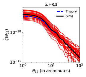
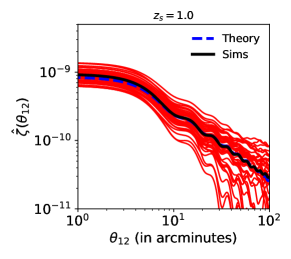
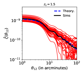
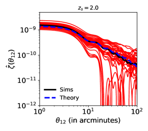
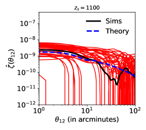
Our theoretical and numerical results are presented in Fig. 1, Fig. 2, Fig. 3 and Fig. 4 respectively for redshifts $z_{s}=0.5,1.0,1.5$ and $2.0$. The thick solid lines in each of these panels correspond to the ensemble average of all maps and the thin solid lines for individual maps. The results for an individual map represent the average of all the patches constructed from that map. The theoretical expectation are shown as dashed lines.

We have also considered realisations of $\kappa$ maps inferred from CMB observations. Our results for all redshifts include the post-Born corrections (PostBorn, ). The post-Born corrections to the 3PCF are included in our modelling of $\zeta(\theta)$, although such corrections do not contribute significantly at lower redshifts (SkewSpec, ; Minkowski, ). The lensing signal for $z_{s}=1100$ is rather weak, but we get reasonable results for small angular scales. For large angular scales the recovered $\zeta$ shows large fluctuations. The results are presented in Fig. 5.

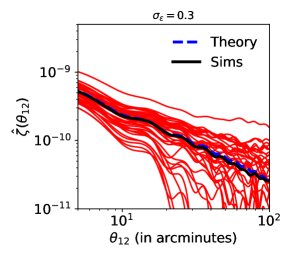
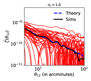
In addition to the noise-free all-sky simulations we have also considered maps at source redshift $z_{s}=1.0$ and applied the pseudo-Euclid mask (see (SkewSpec, ; Minkowski, ) for a detailed description). This mask removes both the galactic and elliptic planes thus leaving roughly $f_{\rm sky}=0.35$ for science exploitation. We also add two different levels of Gaussian noise. The noise power spectrum denoted as $n_{\ell}$ for the noise is given by $n_{\ell}={\sigma^{2}_{\epsilon}/\bar{N}}$. For Euclid we have taken $\bar{n}=30\;{\rm arcmin}^{-2}$. We have considered two values for $\sigma_{\epsilon}$. The results for $\sigma_{\epsilon}=0.3$ are shown in (Fig. 6) and for $\sigma_{\epsilon}=1.0$. in (Fig. 7). As expected the results of comparison of theoretical and numerical results are in agreement with noise free case. The addition of noise only increases the scatter.

VI Conclusion

Using an estimator designed to probe sq3PCF and state-of-the-art simulations we found that the analytical results can be very accurately recovered from numerical simulation. Our estimator probes the squeezed configuration of the bispectrum.

In previous studies, using a different but related estimator, known also as the binned estimator, it was found (Jungwl, ) that, for other shapes, including e.g. the equilateral shape, the fitting function we have used, provides rather accurate description of the numerical estimates from simulations. However, for squeezed configurations this was not the case. We have presented the corresponding results of analysis in the configuration space in this paper.

For cosmological parameter inference using the position-dependent correlation function or IB, if we make the further assumption that the likelihood has gaussian form, we still require an accurate covariance matrix, and this is a far from trivial issue. Most formalism borrowed from CMB studies use a Gaussian Likelihood or its variants. We notice that recently it was shown that a Gaussian approximation is sufficient for the power spectrum (Upham, ) and one-point third-order moment (PSimon, ) for the aperture mass $\langle M^{3}_{ap}\rangle$. However, similar study for two-point third-order statistics, i.e., $\zeta(\theta_{12})$ or equivalently ${\cal B}_{\ell}$ in the harmonic domain, is currently lacking in the literature.

While the diagonal entries in the covariance matrix can be modelled numerically using relatively few simulations, accurate numerical estimates for the off-diagonal elements require many more realisations than we have currently available.

We have computed the scatter in $\zeta$ represented as $\zeta$ and tabulated $\zeta/\sigma(\zeta)$ in Table-I and Table -II as a function of the separation angle $\theta_{12}$. Two values of $\sigma_{\epsilon}=0.3$ and $1.0$ are considered which correspond to the (S/N) of $11.6$ and $6.24$ respectively. A Euclid-type mask with $f_{sky}$=0.3 was considered and sourced were placed at $z_{s}=1.0$. For $z_{s}=1100$ we get ${\rm(S/N)}=1.8$.

We have also studied the sensitivity of $\zeta$ to cosmological parameters. We have computed $|\delta\zeta|/\sigma(\zeta)$. This is done by constructing $|\delta\zeta|=\zeta_{\Omega+}-\zeta_{\Omega}$ and $|\delta\zeta|=\zeta_{\Omega-}-\zeta_{\Omega}$ as a function of $\theta_{12}$ and $\sigma_{\epsilon}$. Here, $\zeta_{\Omega+}$ and $\zeta_{\Omega-}$ corrrespond respectively to 10% higher and lower value of $\Omega_{M}$. The results are presented in Table-3 for $\Omega_{M}$. Corresponding results for $\sigma_{8}$ are shown in Table-4 The top row corresponds to intrinsic ellipticity distribution parameter $\sigma_{\epsilon}=1.0$ whereas the bottom row corresponds to $\sigma_{\epsilon}=0.3$. The total $\rm(S/N)$, for 10% deviation in can be as high as $5.5$ for $\sigma_{8}$.

At the time of writing this paper, we found a similar study (Halder, ) in which the authors consider the squeezed 3PCF for shear using compensated filter and compare the results from simulation against analytic prediction using an older fitting function for the matter bisepctrum.

References

- (1) Planck 2018 results. VI. Cosmological parameters, Planck Collaboration, [arxiv/1807.06209]
- (2) Beyond the Cosmological Standard Model, A. Joyce, B. Jain, J. Khoury, M. Trodden, 2015, Phys. Rep., 568, 1 [astro-ph/1407.0059]
- (3) Modified Gravity and Cosmology, T. Clifton, P. G. Ferreira, A. Padilla, S. Skordis, 2012, Phys. Rep., 513, 1, 1 [astro-ph/1106.2476]
- (4) Massive neutrinos and cosmology, J. Lesgourgues, S. Pastor, 2006, Phys. Rep., 429, 307, [astro-ph/1610.02956]
- (5) The Hyper Suprime-Cam SSP Survey: Overview and Survey Design Aihara H. et al., 2018, Publications of the Astronomical Society of Japan, Volume 70, Issue SP1, S4; [arXiv/1704.05858]
- (6) Cosmology from Cosmic Shear with DES Science Verification Data, The Dark Energy Survey Collaboration, T Abbott, F. B. Abdalla, S. Allam, et al., 2016, Phys. Rev. D, 94, 022001 [arxiv/1507.0552]
- (7) Gravitational Lensing Analysis of the Kilo Degree Survey, K. Kuijken, C. Heymans, H. Hildebrandt, et al., 2015, MNRAS, 454, 3500 [astro-ph/1507.00738]
- (8) Euclid Definition Study Report, R. Laureijs, J. Amiaux, S. Arduini, et al. 2011, ESA/SRE(2011)12.
- (9) LSST: a complementary probe of dark energy, J. A. Tyson, D. M. Wittman, J. F. Hennawi, D. N Spergel, 2003, Nuclear Physics B Proceedings Supplements, 124, 21 [astro-ph/0209632]
- (10) National Research Council. 2010. New Worlds, New Horizons in Astronomy and Astrophysics. The National Academies Press. https://doi.org/10.17226/12951.
- (11) Large scale structure of the universe and cosmological perturbation theory, F. Bernardeau, S. Colombi, E. Gaztanaga, R. Scoccimarro, 2002, Phys.Rep. 367, 1 [astro-ph/0112551]
- (12) Position-dependent correlation function from the SDSS-III Baryon Oscillation Spectroscopic Survey Data Release 10 CMASS Sample, C.-T. Chiang, C. Wagner, A. G. Sánchez, F. Schmidt, E. Komatsu 2015, JCAP, 09, 028 [astro-ph/1504.03322]
- (13) The WiggleZ Dark Energy Survey: Survey Design and First Data Release Michael J. Drinkwater, et al. [arXiv/0911.4246]
- (14) Large-Scale Galaxy Bias, V. Desjacques, D. Jeong, F. Schmidt, 2018, Phys. Rep. 733, 1 [arXiv/1611.09787]
- Castro (2002) Weak lensing analysis in three dimensions, P. G. Castro, A. F. Heavens, T. D. Kitching, 2005, Phys Rev D, 72, 3516 [astro-ph/0503479]
- (16) Higher-order Statistics of Weak Lensing Shear and Flexion, D. Munshi, J. Smidt, A. Heavens, P. Coles, A. Cooray 2011, MNRAS, 411, 2241 [astro-ph/1003.5003]
- (17) Higher-order Convergence Statistics for Three-dimensional Weak Gravitational Lensing, D. Munshi, A. Heavens, P. Coles, 2011, MNRAS, 411, 2161 [astro-ph/1002.2089]
- (18) Higher Order Statistics for Three-dimensional Shear and Flexion, D. Munshi, T. Kitching, A. Heavens, P. Coles, 2011, MNRAS, 416, 629 [astro-ph/1012.3658]
- (19) On the estimation of gravity-induced non-Gaussianities from weak lensing surveys, P. Valageas, D. Munshi, A. J. Barber, 2005, MNRAS. 356, 386 [astro-ph/0402227]
- (20) Weak lensing shear and aperture-mass from linear to non-linear scales, D. Munshi, P. Valageas, A. J. Barber, 2004, MNRAS 350, 77 [astro-ph/0309698]
- (21) From linear to non-linear scales: analytical and numerical predictions for the weak lensing convergence, A. J. Barber, D. Munshi, P. Valageas, 2004, MNRAS, 347, 667 [astro-ph/0304451]
- (22) Statistics of Weak Lensing at Small Angular Scales: Analytical Predictions for Lower Order Moments, D. Munshi, B. Jain, 2001, MNRAS, 322, 107 [astro-ph/9912330]
- (23) Probing The Gravity Induced Bias with Weak Lensing: Test of Analytical results Against Simulations, D. Munshi, 2000, MNRAS, 318, 145 [astro-ph/0001240]
- (24) A New Approach to Probing Primordial Non-Gaussianity, D. Munshi, A. Heavens, 2010, MNRAS, 401, 2406 [arxive/0904.4478]
- (25) Detecting Bispectral Acoustic Oscillations from Inflation Using a New Flexible Estimator, M. Bucher, B. Van Tent, C. S. Carvalho, 2010, MNRAS, 407, 2193 [arXiv/911.1642]
- (26) The binned bispectrum estimator: template-based and non-parametric CMB non-Gaussianity searches, M. Bucher, B. Racine, B. van Tent, 2016, JCAP 1605, 055, [arXiv/1509.08107]
- (27) The Weak Lensing Bispectrum Induced By Gravity, D. Munshi, T. Namikawa, T. Kitching, J. McEwen, R. Takahashi, F. Bouchet et al., 2020, MNRAS, 493, 3985, [arXiv/1910.04627]
- (28) New Optimised Estimators for the Primordial Trispectrum, D. Munshi, A. Heavens, A. Cooray, J. Smidt, P. Coles, P. Serra, 2011, MNRAS, 412, 1993 [arxive/0910.3693]
- (29) Morphology of Weak Lensing Convergence Maps, D. Munshi, T. Namikawa, J. D. McEwen, T. D. Kitching and F. R. Bouchet, [arXiv/2010.05669]
- (30) The Statistics of Weak Lensing at Small Angular Scales: Probability Distribution Function, D. Munshi, B. Jain, 2000, MNRAS, 318, 109 [astro-ph/9911502]
- (31) Testing Inflation with Large Scale Structure: Connecting Hopes with Reality, M. Alvarez et al., [arXiv/1412.4671]
- (32) Analytical Predictions for Statistics of Cosmic Shear: Tests Against Simulations, P. Valageas, A. J. Barber, D. Munshi 2004, MNRAS, 347, 654 [astro-ph/0303472]
- (33) M. Rizzato, K. Benabed, F. Bernardeau and F. Lacasa, Tomographic weak lensing bispectrum: a thorough analysis towards the next generation of galaxy surveys, Mon. Not. R. Astr. Soc. 490 (2019) 4688 [1812.07437]. [arXiv/1812.07437]
- (34) Cosmological parameters from lensing power spectrum and bispectrum tomography M. Takada, B. Jain 2004, MNRAS, 348, 3, 897 [astro-ph/0310125]
- (35) Information content of weak lensing power spectrum and bispectrum: including the non-Gaussian error covariance matrix I. Kayo, M. Takada, B. Jain 2013, MNRAS 429, 344 [arxiv/1207.6322]
- (36) Impact of the non-Gaussian covariance of the weak lensing power spectrum and bispectrum on cosmological parameter estimation M. Sato, T. Nishimichi PRD, 87, 12, 123538 [arxiv/11301.3588]
- (37) Constraints on the dark matter and dark energy interactions from weak lensing bispectrum tomography R. An, C. Feng, B. Wang 2017, JCAP, 10, 049 [arxiv/1706.02845]
- (38) Weak Lensing Minima and Peaks: Cosmological Constraints and the Impact of Baryons W. R. Coulton, J. Liu, I. G. McCarthy, K. Osato 2020, MNRAS, 495, 2531 [arxiv/1910.04171]
- (39) S. Pyne and B. Joachimi, Self-calibration of weak lensing systematic effects using combined two- and three-point statistics, [arXiv/2010.00614]
- (40) Bayesian forward modelling of cosmic shear data, N. Porqueres, A. Heavens, D. Mortlock and G. Lavaux, arXiv e-prints (2020) arXiv:2011.07722 [2011.07722]. [arXiv/2011.07722]
- (41) Likelihood-free inference with neural compression of DES SV weak lensing map statistics, N. Jeffrey, J. Alsing and F. Lanusse, Mon. Not. Roy. Astron. Soc. 501 (2021) 954 [arXiv/2009.08459]
- (42) Position-dependent power spectrum: a new observable in the large-scale structure, C.-T. Chiang, [arXiv/1508.03256]
- (43) The Integrated Bispectrum and Beyond, D. Munshi, P. Coles, 2017, JCAP, 02, 010 [arxive/1608.04345]
- (44) The Integrated Bispectrum in Modified Gravity Theories, D. Munshi, 2017, JCAP, 01, 049 [arXiv/1610.02956]
- (45) Position-dependent power spectra of the 21-cm signal from the epoch of reionization S. K. Giri, A. DÁloisio, G. Mellema, E. Komatsu, R. Ghara, S. Majumdar [arXiv/1811.09633]
- (46) The integrated angular bispectrum G. Jung, F. Oppizzi, A. Ravenni, M. Liguori [arXiv/2004.03574]
- (47) The Lyman- power spectrum - CMB lensing convergence cross-correlation, C.-T. Chiang, A. Slosar, 2018, JCAP, 01, 012 [arXiv/1708.07512]
- (48) Response approach to the squeezed-limit bispectrum: application to the correlation of quasar and Lyman- forest power spectrum, C.-T. Chiang, A. M. Cieplak, F. Schmidt, A. Slosar, 2017, JCAP, 06, 022 [arXiv/1701.03375]
- (49) The integrated angular bispectrum of weak lensing G. Jung, T. Namikawa, M. Liguori, D. Munshi, A. Heavens [arXiv/2102.05521]
- (50) D. Munshi, P. Valageas, L. van Waerbeke, A. Heavens, Cosmology with weak lensing surveys, 2008, Physics Report, 462, 67 [astro-ph/0612667]
- (51) Fitting the nonlinear matter bispectrum by the Halofit approach R. Takahashi, T. Nishimichi, T. Namikawa, A. Taruya, I. Kayo, K. Osato, Y. Kobayashi, M. Shirasaki [arXiv/2102.05521] 2020, ApJ, 895, 113
- (52) Impact of post-Born lensing on the CMB Geraint Pratten, Antony Lewis [arXiv/1605.05662] 2016, JCAP, 1608, 047
- (53) R. Takahashi, T. Hamana, M. Shirasaki, T. Namikawa, T. Nishimichi, K. Osato et al., Full-sky Gravitational Lensing Simulation for Large-area Galaxy Surveys and Cosmic Microwave Background Experiments, Astrophys. J. 850 (2017) 24 [1706.01472]. [arXiv/1706.01472]
- (54) The skewness of the aperture mass statistic Jarvis, M.; Bernstein, G.; Jain, B. 2004, MNRAS, 352, 338 https://arxiv.org/abs/astro-ph/0307393
- (55) K. Gorski, E. Hivon, A. Banday, B. Wandelt, F. Hansen, M. Reinecke et al., HEALPix - A Framework for high resolution discretization, and fast analysis of data distributed on the sphere, 2005, Astrophys. J. 622 (2005) 759 [astro-ph/0409513]
- (56) Weak Lensing Skew-Spectrum, D. Munshi, T. Namikawa, T. D. Kitching, J. D. McEwen, F. R. Bouchet, 2020, MNRAS, 498, 6057, [arXiv/2006.12832]
- (57) The integrated 3-point correlation function of cosmic shear A. Halder, O. Friedrich, S. Seitz, T. N. Varga [arXiv/2102.10177]
- (58) Sufficiency of a Gaussian power spectrum likelihood for accurate cosmology from upcoming weak lensing surveys R. E. Upham, M. L. Brown, L. Whittaker 2021, MNRAS, 503, 1999 [arxiv/2012.06267]
- (59) CFHTLenS: A Gaussian likelihood is a sufficient approximation for a cosmological analysis of third-order cosmic shear statistics P. Simon et al 2015, MNRAS, 449, 1505 [arxiv/1502.04575]