Multilevel Iteration Method for Binary Stochastic Transport Problems

Abstract

This paper presents an iteration method for solving linear particle transport problems in binary stochastic mixtures. It is based on nonlinear projection approach. The method is defined by a hierarchy of equations consisting of the high-order transport equation for materials, low-order Yvon-Mertens equations for conditional ensemble average of the material partial scalar fluxes, and low-order quasidiffusion equations for the ensemble average of the scalar flux and current. The multilevel system of equations is solved by means of an iterative algorithm with the $V$-cycle. The iteration method is analyzed on a set of numerical test problems.

1 Introduction

We consider the Levermore-Pomraning (LP) particle transport model for binary stochastic mixtures (BSM) in 1D slab geometry [1, 2, 3]. The materials are randomly distributed as alternating layers with homogeneous Markov mixing statistics. The mean width of layers of material $\ell$ is equal to $\lambda_{\ell}$. The BSM transport equation with the LP closure in 1D slab geometry is given by

$$\mu\frac{\partial}{\partial x}\Big{(}p_{\ell}\psi_{\ell}(x,\mu)\Big{)}+\sigma_{t,\ell}p_{\ell}\psi_{\ell}(x,\mu)=\frac{1}{2}\sigma_{s,\ell}p_{\ell}\int_{-1}^{1}\psi_{\ell}(x,\mu^{\prime})d\mu^{\prime}\\ +\frac{|\mu|}{\lambda_{\ell^{\prime}}}p_{\ell^{\prime}}\psi_{\ell^{\prime}}(x,\mu)-\frac{|\mu|}{\lambda_{\ell}}p_{\ell}\psi_{\ell}(x,\mu)+\frac{1}{2}p_{\ell}q_{\ell}(x)\,,$$ (1)

$$\ell=1,2\,,\quad\ell^{\prime}\neq\ell\,,\quad x\in[0,X]\,,\quad\mu\in[-1,1]\,$$

with boundary conditions (BCs)

$$\psi_{\ell}\Big{|}_{\stackrel{{\scriptstyle\mu>0}}{{x=0}}}=\psi_{\ell}^{in+}\,,\quad\psi_{\ell}\Big{|}_{\stackrel{{\scriptstyle\mu<0}}{{x=X}}}=\psi_{\ell}^{in-}\,,$$ (2)

where $x$ is the spatial position; $\mu$ is the directional cosine of particle motion; $\psi_{\ell}(x,\mu)$ is the conditional ensemble average (CEA) of the angular flux provided that $x$ is in material $\ell$. $p_{\ell}$ is the probability that the $\ell$-th material is found at a position in the spatial domain. For homogeneous mixing statistics, the probability is given by

$$p_{\ell}=\frac{\lambda_{\ell}}{\lambda_{1}+\lambda_{2}}\,.$$ (3)

The total ensemble average of the angular flux is defined by

$$\big{<}\psi\big{>}\stackrel{{\scriptstyle\Delta}}{{=}}p_{1}\psi_{1}+p_{2}\psi_{2}\,.$$ (4)

The CEA of the scalar flux and current for material $\ell$ are given by

$$\phi_{\ell}\stackrel{{\scriptstyle\Delta}}{{=}}\int_{-1}^{1}\psi_{\ell}d\mu\,,\quad J_{\ell}\stackrel{{\scriptstyle\Delta}}{{=}}\int_{-1}^{1}\mu\psi_{\ell}d\mu\,.$$ (5)

The problems with randomly mixed materials arise in various application, for example, in modeling of inertial confinement fusion targets, nuclear fuel and shielding materials, clouds in atmospheric sciences, tissue in radiation treatment planning [4]. The source iteration scheme for the linear binary stochastic transport equation converges very slow [5, 6]. Various synthetic acceleration methods for this class of particle transport problems have been developed [7, 8, 9, 10, 11]. In this paper, we apply nonlinear projection approach to derive a multilevel iteration method [12, 13]. It is defined by a system of equations consisting of the high-order transport equation and low-order equations for various moments of the transport solution. The iteration method can be interpreted as a nonlinear multigrid method over elements of the phase space. The proposed multilevel method can be applied for radiation transport problems in random media coupled with multiphysics equations [14, 15].

The reminder of the paper is organized as follows. In Sec. 2 the system of low-order equations for transport problems in BSM is formulated. The iteration algorithm is described in Sec. 3. Numerical results are presented in Sec. 4. We conclude with a brief discussion in Sec. 5.

2 Hierarchy of Equations of Multilevel Method for BSM

The multilevel method for solving the BSM transport problem (1) and (2) is formulated by a high-order equation for $\psi_{\ell}$ and low-order equations for moments the CEA of the angular flux with exact closures. To derive the hierarchy of equations of the method we define (i) projection operators at each level, (ii) moments of the transport solution low-order equations are formulated for, and (iii) prolongation operators that enable to couple equations at different levels.

A specific feature of the transport equation (1) for each material is that its right-hand side (RHS) contains terms with absolute value of $\mu$ while the left-hand side (LHS) explicitly depends of $\mu$. A natural way of forming a set of moment equations based on projection of the high-order equation with this structure of terms is to define the low-order equations for half-range moments

$$\phi_{\ell}^{\pm}\stackrel{{\scriptstyle\Delta}}{{=}}\pm\int_{0}^{\pm 1}\psi_{\ell}d\mu$$ (6)

that are the CEA of the partial scalar fluxes. The high-order equation (1) is integrated over $-1\leq\mu\leq 1$ with weights 1 and $\mu$ to obtain the low-order equations for $\phi_{\ell}^{\pm}$ defined by

$$\frac{d}{dx}\big{(}p_{\ell}(C_{\ell}^{+}\phi_{\ell}^{+}+C_{\ell}^{-}\phi_{\ell}^{-})\big{)}+\Big{(}\sigma_{a,\ell}+\frac{C_{\ell}^{+}}{\lambda_{\ell}}\Big{)}p_{\ell}\phi_{\ell}^{+}+\Big{(}\sigma_{a,\ell}-\frac{C_{\ell}^{-}}{\lambda_{\ell}}\Big{)}p_{\ell}\phi_{\ell}^{-}=\\ \frac{p_{\ell^{\prime}}}{\lambda_{\ell^{\prime}}}\big{(}C_{\ell^{\prime}}^{+}\phi_{\ell^{\prime}}^{+}-C_{\ell^{\prime}}^{-}\phi_{\ell^{\prime}}^{-}\big{)}+p_{\ell}q_{\ell}\,,$$ (7a)

$$\frac{d}{dx}\big{(}p_{\ell}(E_{\ell}^{+}\phi_{\ell}^{+}+E_{\ell}^{-}\phi_{\ell}^{-})\big{)}+\Big{(}\sigma_{t,\ell}C_{\ell}^{+}+\frac{E_{\ell}^{+}}{\lambda_{\ell}}\Big{)}p_{\ell}\phi_{\ell}^{+}+\Big{(}\sigma_{t,\ell}C_{\ell}^{-}-\frac{E_{\ell}^{-}}{\lambda_{\ell}}\Big{)}p_{\ell}\phi_{\ell}^{-}=\\ \frac{p_{\ell^{\prime}}}{\lambda_{\ell^{\prime}}}\big{(}E_{\ell^{\prime}}^{+}\phi_{\ell^{\prime}}^{+}-E_{\ell^{\prime}}^{-}\phi_{\ell^{\prime}}^{-}\big{)}\,,$$ (7b)

where the low-order equations are closed by means of the linear-fractional factors defined by

$$C_{\ell}^{\pm}\stackrel{{\scriptstyle\Delta}}{{=}}\frac{\int_{0}^{\pm 1}\mu\psi_{\ell^{\prime}}d\mu}{\int_{0}^{\pm 1}\psi_{\ell}d\mu}\,,\quad E_{\ell}^{\pm}\stackrel{{\scriptstyle\Delta}}{{=}}\frac{\int_{0}^{\pm 1}\mu^{2}\psi_{\ell}d\mu}{\int_{0}^{\pm 1}\psi_{\ell}d\mu}\,.$$ (8)

The CEA of the material partial currents are defined by

$$J^{\pm}_{\ell}\stackrel{{\scriptstyle\Delta}}{{=}}\pm\int_{0}^{\pm 1}\mu\psi_{\ell}d\mu\,.$$ (9)

They are cast in terms of the partial scalar fluxes as follows:

$$J^{\pm}_{\ell}=C^{\pm}_{\ell}\phi^{\pm}_{\ell}\,.$$ (10)

The BCs for Eqs. (7) have the following form:

$$\phi_{\ell}^{+}\Big{|}_{x=0}=\phi_{\ell}^{in,+}\,,\quad\phi_{\ell}^{-}\Big{|}_{x=X}=\phi_{\ell}^{in,-}\,,$$ (11)

where

$$\phi_{\ell}^{in,\pm}\!\stackrel{{\scriptstyle\Delta}}{{=}}\!\pm\int_{0}^{\pm 1}\!\psi_{\ell}^{in,+}d\mu\,.$$ (12)

The low-order equations (7) use the same projection operators and unknowns as the DP₁ equations [16, 17, 18, 19]. They can be viewed as nonlinear DP₁ equations with exact closures. This approach has been applied to formulate Yvon-Mertens (YM) method for the linear Boltzmann equation [20]. Hereafter these equations are referred to as the low-order YM (LOYM) equations.

The BSM transport equation (1) is now projected to formulate low-order equations for the total ensemble averaged scalar flux $\big{<}\phi\big{>}$ and current $\big{<}J\big{>}$, where $\big{<}f\big{>}\stackrel{{\scriptstyle\Delta}}{{=}}p_{1}f_{1}+p_{2}f_{2}$ is the notation for the ensemble average. The equation (1) is summed over materials and then integrated over $-1\leq\mu\leq 1$ with weights 1 and $\mu$ to obtain the low-order quasidiffusion (LOQD) equations for $\big{<}\phi\big{>}$ and $\big{<}J\big{>}$ given by [21]

$$\frac{d\big{<}J\big{>}}{dx}+\big{<}\!\!\big{<}\sigma_{a}\big{>}\!\!\big{>}\big{<}\phi\big{>}=\big{<}q\big{>}\,,$$ (13a)

$$\frac{d}{dx}\Big{(}\big{<}\!\!\big{<}E\big{>}\!\!\big{>}\big{<}\phi\big{>}\Big{)}+\big{<}\!\!\big{<}\sigma_{t}\big{>}\!\!\big{>}\big{<}J\big{>}+\big{<}\!\!\big{<}\eta\big{>}\!\!\big{>}\big{<}\phi\big{>}=0\,,$$ (13b)

$$\big{<}J\big{>}\Big{|}_{x=0}\!\!=\!\!\big{<}\!\!\big{<}C^{-}\big{>}\!\!\big{>}\Big{(}\big{<}\phi\big{>}-\big{<}\phi^{in,+}\big{>}\Big{)}\Big{|}_{x=0}\!\!+\big{<}J^{in,+}\big{>}\,,$$ (14a)

$$\big{<}J\big{>}\Big{|}_{x=X}\!\!=\!\!\big{<}\!\!\big{<}C^{+}\big{>}\!\!\big{>}\Big{(}\big{<}\phi\big{>}-\big{<}\phi^{in,-}\big{>}\Big{)}\Big{|}_{x=X}\!\!+\big{<}J^{in,-}\big{>}\,,$$ (14b)

where the coefficients are defined by means of the LOYM solution as follows:

$$\big{<}\!\!\big{<}\sigma_{a}\big{>}\!\!\big{>}\stackrel{{\scriptstyle\Delta}}{{=}}\frac{\sum_{\ell=1}^{2}\sigma_{a,\ell}p_{\ell}(\phi_{\ell}^{+}+\phi_{\ell}^{-})}{\sum_{\ell=1}^{2}p_{\ell}(\phi_{\ell}^{+}+\phi_{\ell}^{-})}\,,\quad\big{<}\!\!\big{<}\sigma_{t}\big{>}\!\!\big{>}\stackrel{{\scriptstyle\Delta}}{{=}}\frac{\sum_{\ell=1}^{2}\sigma_{t,\ell}p_{\ell}|C_{\ell}^{+}\phi_{\ell}^{+}+C_{\ell}^{-}\phi_{\ell}^{-}|}{\sum_{\ell=1}^{2}p_{\ell}|C_{\ell}^{+}\phi_{\ell}^{+}+C_{\ell}^{-}\phi_{\ell}^{-}|}\,,$$ (15)

$$\big{<}\!\!\big{<}\eta\big{>}\!\!\big{>}\!\stackrel{{\scriptstyle\Delta}}{{=}}\!\frac{\sum_{\ell=1}^{2}\!\big{(}\sigma_{t,\ell}\!-\!\big{<}\!\!\big{<}\sigma_{t}\big{>}\!\!\big{>}\big{)}p_{\ell}(C_{\ell}^{+}\phi_{\ell}^{+}\!+\!C_{\ell}^{-}\phi_{\ell}^{-})}{\sum_{\ell=1}^{2}p_{\ell}(\phi_{\ell}^{+}+\phi_{\ell}^{-})}\,,\quad\big{<}\!\!\big{<}E\big{>}\!\!\big{>}\!\stackrel{{\scriptstyle\Delta}}{{=}}\!\frac{\sum_{\ell=1}^{2}\!p_{\ell}(E_{\ell}^{+}\phi_{\ell}^{+}+E_{\ell}^{-}\phi_{\ell}^{-})}{\sum_{\ell=1}^{2}p_{\ell}(\phi_{\ell}^{+}+\phi_{\ell}^{-})}\,,$$ (16)

$$\big{<}\!\!\big{<}C^{\pm}\big{>}\!\!\big{>}\stackrel{{\scriptstyle\Delta}}{{=}}\frac{\sum_{\ell=1}^{2}C_{\ell}^{\pm}p_{\ell}\phi_{\ell}^{\pm}}{\sum_{\ell=1}^{2}p_{\ell}\phi_{\ell}^{\pm}}\,,\quad J_{\ell}^{in\pm}\stackrel{{\scriptstyle\Delta}}{{=}}\int_{0}^{\pm 1}\mu\psi_{\ell}^{in\pm}d\mu\,.$$ (17)

The next step in formulation of the multilevel system of low-order equations is to define prolongation operators that enable to couple the LOQD and LOYM equations. The term $\frac{p_{\ell}}{\lambda_{\ell^{\prime}}}(C_{\ell}^{+}\phi_{\ell}^{+}-C_{\ell}^{-}\phi_{\ell}^{-})$ is added to the LHS and RHS of Eq. (7a) and $\frac{p_{\ell}}{\lambda_{\ell^{\prime}}}(E_{\ell}^{+}\phi_{\ell}^{+}-E_{\ell}^{-}\phi_{\ell}^{-})$ is added to the LHS and RHS of Eq. (7b) to get

$$\frac{d}{dx}\big{(}p_{\ell}(C_{\ell}^{+}\phi_{\ell}^{+}+C_{\ell}^{-}\phi_{\ell}^{-})\big{)}+\bigg{(}\sigma_{a,\ell}+C_{\ell}^{+}\Big{(}\frac{1}{\lambda_{\ell}}+\frac{1}{\lambda_{\ell^{\prime}}}\Big{)}\bigg{)}p_{\ell}\phi_{\ell}^{+}+\bigg{(}\sigma_{a,\ell}-C_{\ell}^{-}\Big{(}\frac{1}{\lambda_{\ell}}+\frac{1}{\lambda_{\ell^{\prime}}}\Big{)}\bigg{)}p_{\ell}\phi_{\ell}^{-}=\\ \frac{1}{\lambda_{\ell^{\prime}}}\sum_{\ell^{\prime\prime}=1}^{2}p_{\ell^{\prime\prime}}\Big{(}C_{\ell^{\prime\prime}}^{+}\phi_{\ell^{\prime\prime}}^{+}-C_{\ell^{\prime\prime}}^{-}\phi_{\ell^{\prime\prime}}^{-}\Big{)}+p_{\ell}q_{\ell}\,,$$ (18a)

$$\frac{d}{dx}\big{(}p_{\ell}(E_{\ell}^{+}\phi_{\ell}^{+}+E_{\ell}^{-}\phi_{\ell}^{-})\big{)}+\bigg{(}\sigma_{t,\ell}C_{\ell}^{+}+E_{\ell}^{+}\Big{(}\frac{1}{\lambda_{\ell}}+\frac{1}{\lambda_{\ell^{\prime}}}\Big{)}\bigg{)}p_{\ell}\phi_{\ell}^{+}+\bigg{(}\sigma_{t,\ell}C_{\ell}^{-}-E_{\ell}^{-}\Big{(}\frac{1}{\lambda_{\ell}}+\frac{1}{\lambda_{\ell^{\prime}}}\Big{)}\bigg{)}p_{\ell}\phi_{\ell}^{-}=\\ \frac{1}{\lambda_{\ell^{\prime}}}\sum_{\ell^{\prime\prime}=1}^{2}p_{\ell^{\prime}}\Big{(}E_{\ell^{\prime\prime}}^{+}\phi_{\ell^{\prime\prime}}^{+}-E_{\ell^{\prime\prime}}^{-}\phi_{\ell^{\prime\prime}}^{-}\Big{)}\,.$$ (18b)

Taking into account Eq. (10), we obtain

$$\sum_{\ell^{\prime\prime}=1}^{2}p_{\ell^{\prime\prime}}\Big{(}C_{\ell^{\prime\prime}}^{+}\phi_{\ell^{\prime\prime}}^{+}-C_{\ell^{\prime\prime}}^{-}\phi_{\ell^{\prime\prime}}^{-}\Big{)}=\big{<}J^{+}\big{>}-\big{<}J^{-}\big{>}\,.$$ (19)

We define

$$\big{<}\!\!\big{<}E^{\pm}\big{>}\!\!\big{>}\stackrel{{\scriptstyle\Delta}}{{=}}\frac{\sum_{\ell=1}^{2}E_{\ell}^{\pm}p_{\ell}\phi_{\ell}^{\pm}}{\sum_{\ell=1}^{2}p_{\ell}\phi_{\ell}^{\pm}}\,$$ (20)

to get

$$\sum_{\ell^{\prime\prime}=1}^{2}p_{\ell^{\prime\prime}}\Big{(}E_{\ell^{\prime\prime}}^{+}\phi_{\ell^{\prime\prime}}^{+}-E_{\ell^{\prime\prime}}^{-}\phi_{\ell^{\prime\prime}}^{-}\Big{)}=\big{<}\!\!\big{<}E^{+}\big{>}\!\!\big{>}\big{<}\phi^{+}\big{>}-\big{<}\!\!\big{<}E^{-}\big{>}\!\!\big{>}\big{<}\phi^{-}\big{>}\,.$$ (21)

Using Eqs. (19) and (21) in Eq. (18), we obtain the modified LOYM equations of the following form:

$$\frac{d}{dx}\big{(}p_{\ell}(C_{\ell}^{+}\phi_{\ell}^{+}+C_{\ell}^{-}\phi_{\ell}^{-})\big{)}+\bigg{(}\sigma_{a,\ell}+C_{\ell}^{+}\Big{(}\frac{1}{\lambda_{\ell}}+\frac{1}{\lambda_{\ell^{\prime}}}\Big{)}\bigg{)}p_{\ell}\phi_{\ell}^{+}+\bigg{(}\sigma_{a,\ell}-C_{\ell}^{-}\Big{(}\frac{1}{\lambda_{\ell}}+\frac{1}{\lambda_{\ell^{\prime}}}\Big{)}\bigg{)}p_{\ell}\phi_{\ell}^{-}=\\ \frac{1}{\lambda_{\ell^{\prime}}}\Big{(}\big{<}J^{+}\big{>}-\big{<}J^{-}\big{>}\Big{)}+p_{\ell}q_{\ell}\,,$$ (22a)

$$\frac{d}{dx}\big{(}p_{\ell}(E_{\ell}^{+}\phi_{\ell}^{+}+E_{\ell}^{-}\phi_{\ell}^{-})\big{)}+\bigg{(}\sigma_{t,\ell}C_{\ell}^{+}+E_{\ell}^{+}\Big{(}\frac{1}{\lambda_{\ell}}+\frac{1}{\lambda_{\ell^{\prime}}}\Big{)}\bigg{)}p_{\ell}\phi_{\ell}^{+}+\bigg{(}\sigma_{t,\ell}C_{\ell}^{-}-E_{\ell}^{-}\Big{(}\frac{1}{\lambda_{\ell}}+\frac{1}{\lambda_{\ell^{\prime}}}\Big{)}\bigg{)}p_{\ell}\phi_{\ell}^{-}=\\ \frac{1}{\lambda_{\ell^{\prime}}}\Big{(}\big{<}\!\!\big{<}E^{+}\big{>}\!\!\big{>}\big{<}\phi^{+}\big{>}-\big{<}\!\!\big{<}E^{-}\big{>}\!\!\big{>}\big{<}\phi^{-}\big{>}\Big{)}\,.$$ (22b)

The prolongation operators that enable one to map $\big{<}\phi\big{>}$ and $\big{<}J\big{>}$ to $\big{<}\phi^{\pm}\big{>}$ and $\big{<}J^{\pm}\big{>}$ are defined as follows [22]:

$$\big{<}\phi^{\pm}\big{>}=\big{<}\!\!\big{<}\beta^{\pm}\big{>}\!\!\big{>}\Big{(}\big{<}J\big{>}-\big{<}\!\!\big{<}\tilde{C}^{\pm}\big{>}\!\!\big{>}\big{<}\phi\big{>}\Big{)}\,,\quad\big{<}J^{\pm}\big{>}=\big{<}\!\!\big{<}\gamma^{\pm}\big{>}\!\!\big{>}\Big{(}\big{<}J\big{>}-\big{<}\!\!\big{<}\tilde{C}^{\pm}\big{>}\!\!\big{>}\big{<}\phi\big{>}\Big{)}\,,$$ (23)

where

$$\big{<}\!\!\big{<}\beta^{\pm}\big{>}\!\!\big{>}\stackrel{{\scriptstyle\Delta}}{{=}}\frac{\sum_{\ell=1}^{2}p_{\ell}\phi_{\ell}^{\pm}}{\sum_{\ell=1}^{2}(C_{\ell}^{\pm}-C_{\ell}^{\mp})p_{\ell}\phi_{\ell}^{\pm}}\,,\quad\big{<}\!\!\big{<}\gamma^{\pm}\big{>}\!\!\big{>}\stackrel{{\scriptstyle\Delta}}{{=}}\frac{\sum_{\ell=1}^{2}C_{\ell}^{\pm}p_{\ell}\phi_{\ell}^{\pm}}{\sum_{\ell=1}^{2}(C_{\ell}^{\pm}-C_{\ell}^{\mp})p_{\ell}\phi_{\ell}^{\pm}}\,,$$ (24)

and

$$\big{<}\!\!\big{<}\tilde{C}^{\pm}\big{>}\!\!\big{>}\stackrel{{\scriptstyle\Delta}}{{=}}\frac{\sum_{\ell=1}^{2}C_{\ell}^{\pm}p_{\ell}(\phi_{\ell}^{+}+\phi_{\ell}^{-})}{\sum_{\ell=1}^{2}p_{\ell}(\phi_{\ell}^{+}+\phi_{\ell}^{-})}\,.$$ (25)

To formulate the high-order transport equation of the multilevel method, we cast the RHS of Eq. (1) in terms of $\phi_{\ell}$ to obtain the equation for $\psi_{\ell}$ given by

$$\mathcal{L}_{\ell}p_{\ell}\psi_{\ell}=\frac{1}{2}\sigma_{s,\ell}p_{\ell}\phi_{\ell}+\frac{|\mu|}{\lambda_{\ell^{\prime}}}p_{\ell^{\prime}}\psi_{\ell^{\prime}}+\frac{1}{2}p_{\ell}q_{\ell}\,,\ \ell^{\prime}\neq\ell\,,$$ (26)

$$\mathcal{L}_{\ell}\stackrel{{\scriptstyle\Delta}}{{=}}\mu\frac{\partial}{\partial x}+\Big{(}\sigma_{t,\ell}+\frac{|\mu|}{\lambda_{\ell}}\Big{)}\,.$$ (27)

3 Multilevel Iteration Scheme

The multilevel iteration method for transport problems in BSM is defined by several stages which involve solving the following equations at different levels:

• the high-order transport equation (26) for $\psi_{\ell}$,

• the LOYM equations (7) and (11) for $\phi^{\pm}_{\ell}$,

• the LOQD equations (13) and (14) for $\big{<}\phi\big{>}$ and $\big{<}J\big{>}$,

• the modified LOYM equations (22) and (11) for $\phi^{\pm}_{\ell}$.

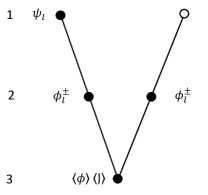
This method is a nonlinear multigrid scheme over elements of the phase space. On each transport iteration, the hierarchy of equations is solved according to the $V$-cycle illustrated in Figure 1. The detailed iteration scheme is presented in Algorithm 1, where $s$ is the index of transport iterations.

Figure 1: $V$-cycle

The high-order transport equation (26) for material $\ell$ depends on the CEA of the angular flux of another material $\ell^{\prime}$. The LOYM equations (7) for material $\ell$ also contain terms with the partial scalar fluxes and factors of material $\ell^{\prime}$. In this paper, fully iterative approach is studied. The multilevel method executes relaxation cycles at the level of the material high-order equations using Gauss-Seidel (GS) iterations. The scattering term is defined by the material scalar fluxes obtained from the low-order problems. $n$ is the index of inner GS iterations. The number of GS cycles equals $n_{max}$. The same approach is applied to solve coupled material LOYM equations (7). At this level, only one GS iteration over the material LOYM equations is performed. The modified LOYM equations (22) for materials are decoupled due to the prolongation operator that defines the RHS. There are no inner iterations at this stage.

To discretize the high-order transport equation (26) the linear discontinuous (LD) finite element method is used. The LOYM and LOQD equations are discretized consistently with the LD scheme for Eq. (26) [22].

$s=0$

while $||\big{<}\phi\big{>}^{(s)}-\big{<}\phi\big{>}^{(s-1)}||_{\infty}>\epsilon||\big{<}\phi\big{>}^{(s)}||_{\infty}$  do

       $s=s+1$ ,   $n=0$ ,  $\psi_{2}^{(0,s+1/3)}=\psi_{2}^{(s)}$

       Level 1: high-order transport problem for materials

       while $n\leq n_{max}$  do

             $n=n+1$

             $\mathcal{L}_{1}p_{1}\psi_{1}^{(n,s+1/3)}=|\mu|\lambda_{2}^{-1}p_{2}\psi_{2}^{(n-1,s+1/3)}+0.5\sigma_{s,1}p_{1}\phi_{1}^{(s)}+0.5p_{1}q_{1}$

             $\mathcal{L}_{2}p_{2}\psi_{2}^{(n,s+1/3)}=|\mu|\lambda_{1}^{-1}p_{1}\psi_{1}^{(n,s+1/3)}\quad+0.5\sigma_{s,2}p_{2}\phi_{2}^{(s)}+0.5p_{2}q_{2}$

            

      $\psi_{\ell}^{(s+1/3)}\leftarrow\psi_{\ell}^{(n_{max},s+1/3)}$

       Compute $C_{\ell}^{\pm(s+1/3)}$ and $E_{\ell}^{\pm(s+1/3)}$ ($\ell=1,2$), $\phi_{2}^{\pm(s+1/3)}$

       Level 2: low-order problem for materials

       Perform one GS material iteration to solve LOYM eqs. (7) for $\phi_{\ell}^{\pm(s+2/3)}$ with $\phi_{2}^{\pm(s+1/3)}$ as an initial guess

       Compute $\!\big{<}\!\!\big{<}\beta^{\pm}\big{>}\!\!\big{>}^{\!(s+2/3)}$, $\big{<}\!\!\big{<}\gamma^{\pm}\big{>}\!\!\big{>}^{\!(s+2/3)}$, $\big{<}\!\!\big{<}\tilde{C}^{\pm}\big{>}\!\!\big{>}^{\!(s+2/3)}$, $\big{<}\!\!\big{<}E^{\pm}\big{>}\!\!\big{>}^{\!(s+2/3)}$, $\big{<}\!\!\big{<}\sigma_{a}\big{>}\!\!\big{>}^{(s+2/3)}$, $\big{<}\!\!\big{<}\sigma_{t}\big{>}\!\!\big{>}^{(s+2/3)}$, $\big{<}\!\!\big{<}\eta\big{>}\!\!\big{>}^{(s+2/3)}$, $\big{<}\!\!\big{<}E\big{>}\!\!\big{>}^{(s+2/3)}$, $\big{<}\!\!\big{<}C^{\pm}\big{>}\!\!\big{>}^{(s+2/3)}$

       Level 3: low-order problem for total ensemble average moments

       Solve LOQD eqs. (13) for $\big{<}\phi\big{>}^{(s+1)}$ and $\big{<}J\big{>}^{(s+1)}$

       Compute $\big{<}\phi^{\pm}\big{>}^{(s+2/3)}$ and $\big{<}J^{\pm}\big{>}^{(s+2/3)}$

       Level 2: low-order problem for materials

       Solve LOYM eqs. (22) for $\phi_{\ell}^{\pm(s+1)}$

       Compute $\!\big{<}\!\!\big{<}\beta^{\pm}\big{>}\!\!\big{>}^{\!(s+1)}$, $\big{<}\!\!\big{<}\gamma^{\pm}\big{>}\!\!\big{>}^{\!(s+1)}$, $\big{<}\!\!\big{<}\tilde{C}^{\pm}\big{>}\!\!\big{>}^{\!(s+1)}$, $\big{<}\!\!\big{<}E^{\pm}\big{>}\!\!\big{>}^{\!(s+1)}$

       Compute $\big{<}\phi^{\pm}\big{>}^{(s+1)}$ and $\big{<}J^{\pm}\big{>}^{(s+1)}$

       Prolongation

       $\phi_{\ell}^{(s+1)}\leftarrow(\phi_{\ell}^{-(s+1)}+\phi_{\ell}^{+(s+1)})\big{<}\phi\big{>}^{(s+1)}\big{/}\sum_{\ell^{\prime}=1}^{2}p_{\ell^{\prime}}\big{(}\phi_{\ell^{\prime}}^{-(s+1)}+\phi_{\ell^{\prime}}^{+(s+1)}\big{)}$

       $\tilde{\phi}^{\pm(s+1)}_{\ell}\leftarrow\phi_{\ell}^{\pm(s+1)}\big{<}\phi^{\pm}\big{>}^{(s+1)}\big{/}\sum_{\ell^{\prime}=1}^{2}p_{\ell^{\prime}}\phi_{\ell^{\prime}}^{\pm(s+1)}$

       $\psi_{\ell}^{(s+1)}\leftarrow\pm\psi_{\ell}^{(s+1/3)}\tilde{\phi}_{\ell}^{\pm(s+1)}\big{/}\int_{0}^{\pm 1}\psi_{\ell}^{(s+1/3)}d\mu^{\prime}$,  $\mu\gtrless 0$

      

Algorithm 1 The multilevel iteration method for the BSM transport equation

4 Numerical Results

To analyze the multilevel iteration method we use four sets of numerical test problems [2]. The data for the tests are presented in Table 1. The problems are defined for a slab $0\leq x\leq 100$ with vacuum boundaries. The spatial mesh is uniform with 100 cells. The double $S_{4}$ Gauss-Legendre quadrature set is used. The sets of tests differ from each other by values of $\lambda_{\ell}\sigma_{t,\ell}$. The problems in each set have materials with different scattering ratios as well as total cross sections.

Table 1: Data for Test Problems

Test	$\sigma_{t,1}$	$\frac{\sigma_{s,1}}{\sigma_{t,1}}$	$\lambda_{1}$	$q_{1}$	$\sigma_{t,2}$	$\frac{\sigma_{s,2}}{\sigma_{t,2}}$	$\lambda_{2}$	$q_{1}$	$\lambda_{1}\sigma_{t,1}$	$\lambda_{2}\sigma_{t,2}$
A1	$\frac{10}{99}$	0	$\frac{99}{100}$	1	$\frac{100}{11}$	1	$\frac{11}{100}$	1	0.1	1
A2	$\frac{10}{99}$	1	$\frac{99}{100}$	1	$\frac{100}{11}$	0	$\frac{11}{100}$	1	0.1	1
A3	$\frac{10}{99}$	0.9	$\frac{99}{100}$	1	$\frac{100}{11}$	0.9	$\frac{11}{100}$	1	0.1	1
B1	$\frac{10}{99}$	0	$\frac{99}{10}$	1	$\frac{100}{11}$	1	$\frac{11}{10}$	1	1	10
B2	$\frac{10}{99}$	1	$\frac{99}{10}$	1	$\frac{100}{11}$	0	$\frac{11}{10}$	1	1	10
B3	$\frac{10}{99}$	0.9	$\frac{99}{10}$	1	$\frac{100}{11}$	0.9	$\frac{11}{10}$	1	1	10
C1	$\frac{2}{101}$	0	$\frac{101}{20}$	1	$\frac{200}{101}$	1	$\frac{101}{20}$	1	0.1	10
C2	$\frac{2}{101}$	1	$\frac{101}{20}$	1	$\frac{200}{101}$	0	$\frac{101}{20}$	1	0.1	10
C3	$\frac{2}{101}$	0.9	$\frac{101}{20}$	1	$\frac{200}{101}$	0.9	$\frac{101}{20}$	1	0.1	10
D1	$\frac{1}{99}$	0	$\frac{99}{100}$	1	$\frac{10}{11}$	1	$\frac{11}{10}$	1	0.01	1
D2	$\frac{1}{99}$	1	$\frac{99}{100}$	1	$\frac{10}{11}$	0	$\frac{11}{10}$	1	0.01	1
D3	$\frac{1}{99}$	0.9	$\frac{99}{100}$	1	$\frac{10}{11}$	0.9	$\frac{11}{10}$	1	0.01	1

Table 2: Numerically Estimated Spectral Radii

$n_{max}$	A1	A2	A3	B1	B2	B3	C1	C2	C3	D1	D2	D3
1	0.4	0.41	0.41	0.23	0.12	0.12	0.11	0.06	0.10	0.46	0.43	0.46
2	0.16	0.17	0.16	0.25	0.12	0.1	0.14	0.03	0.11	0.19	0.20	0.21

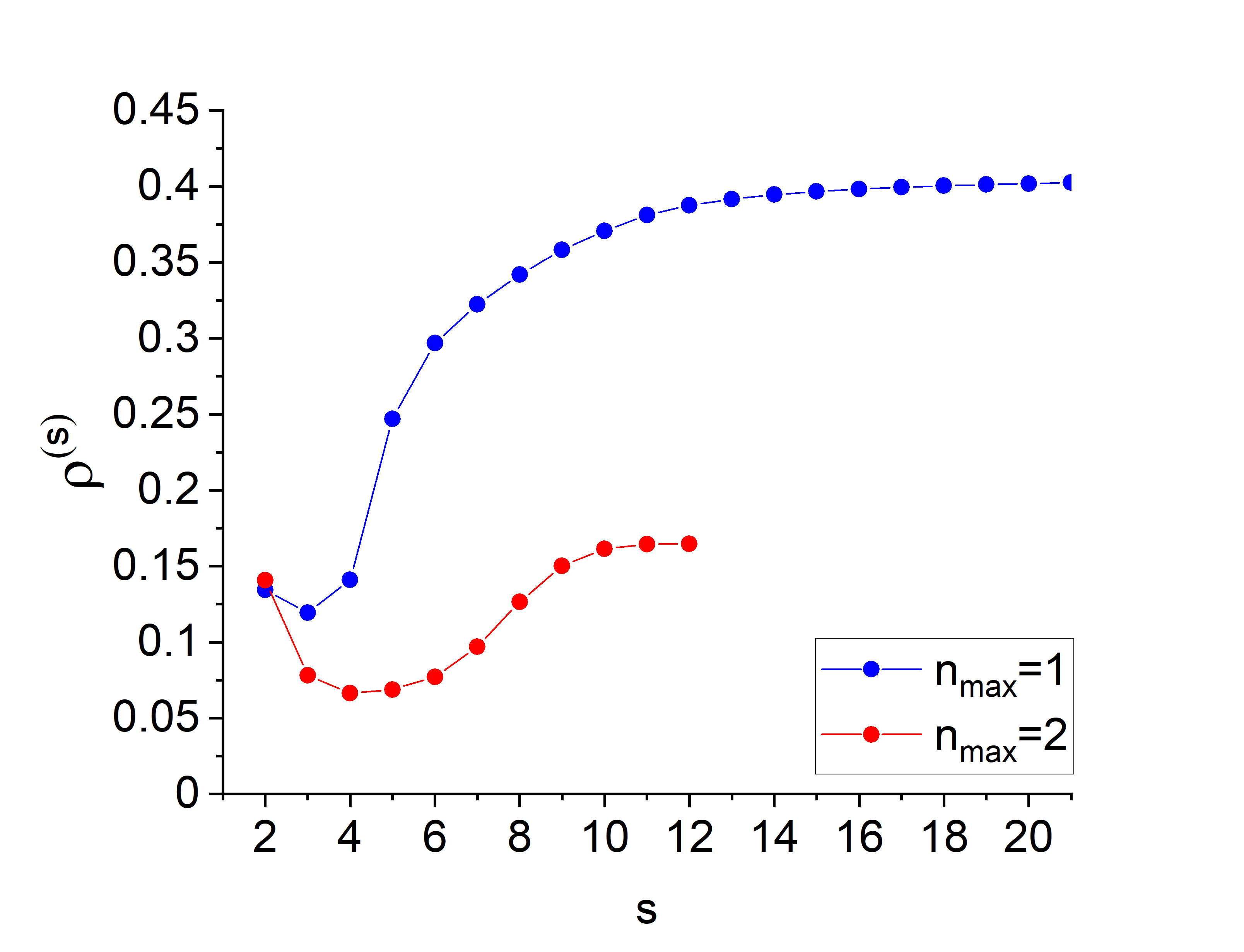
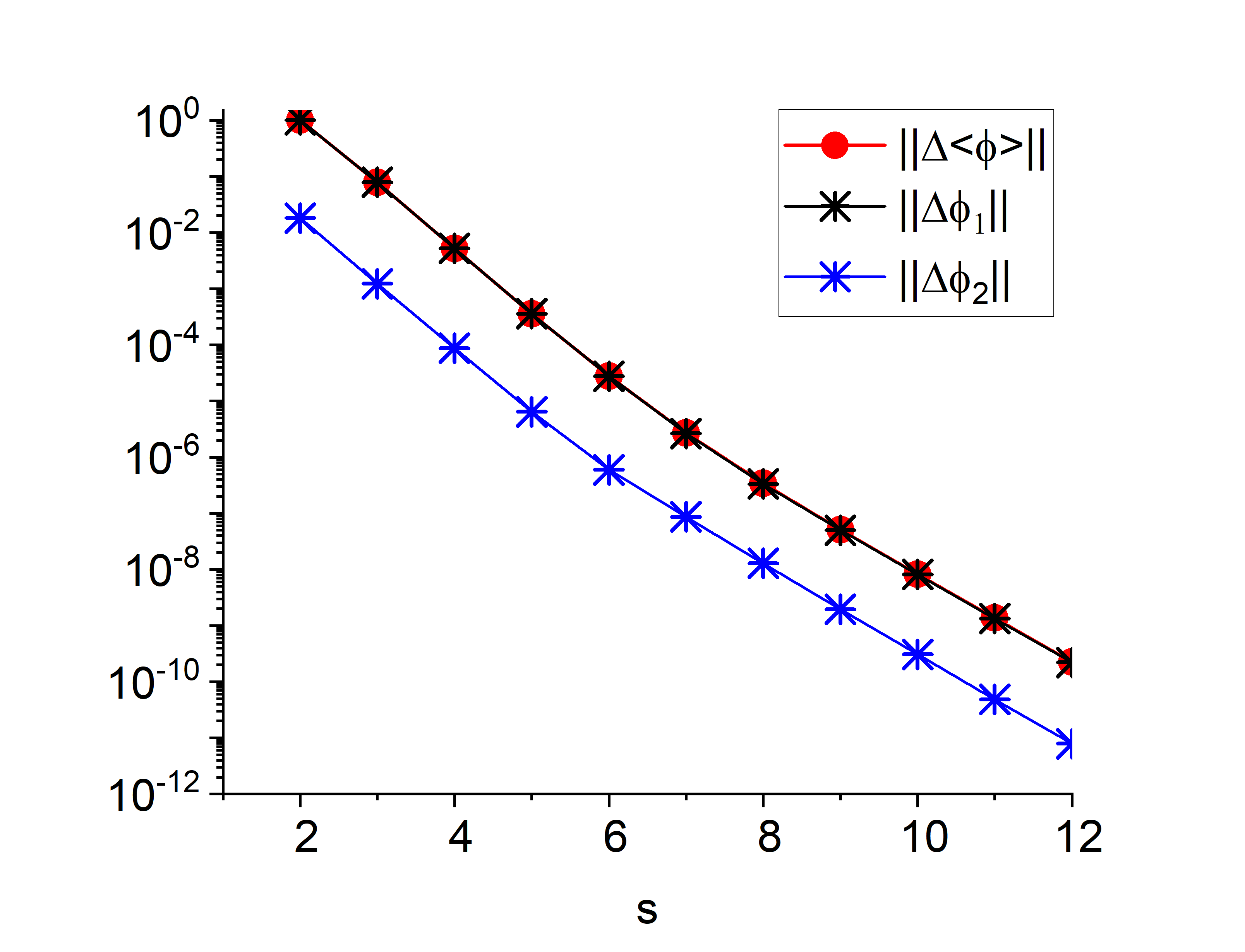
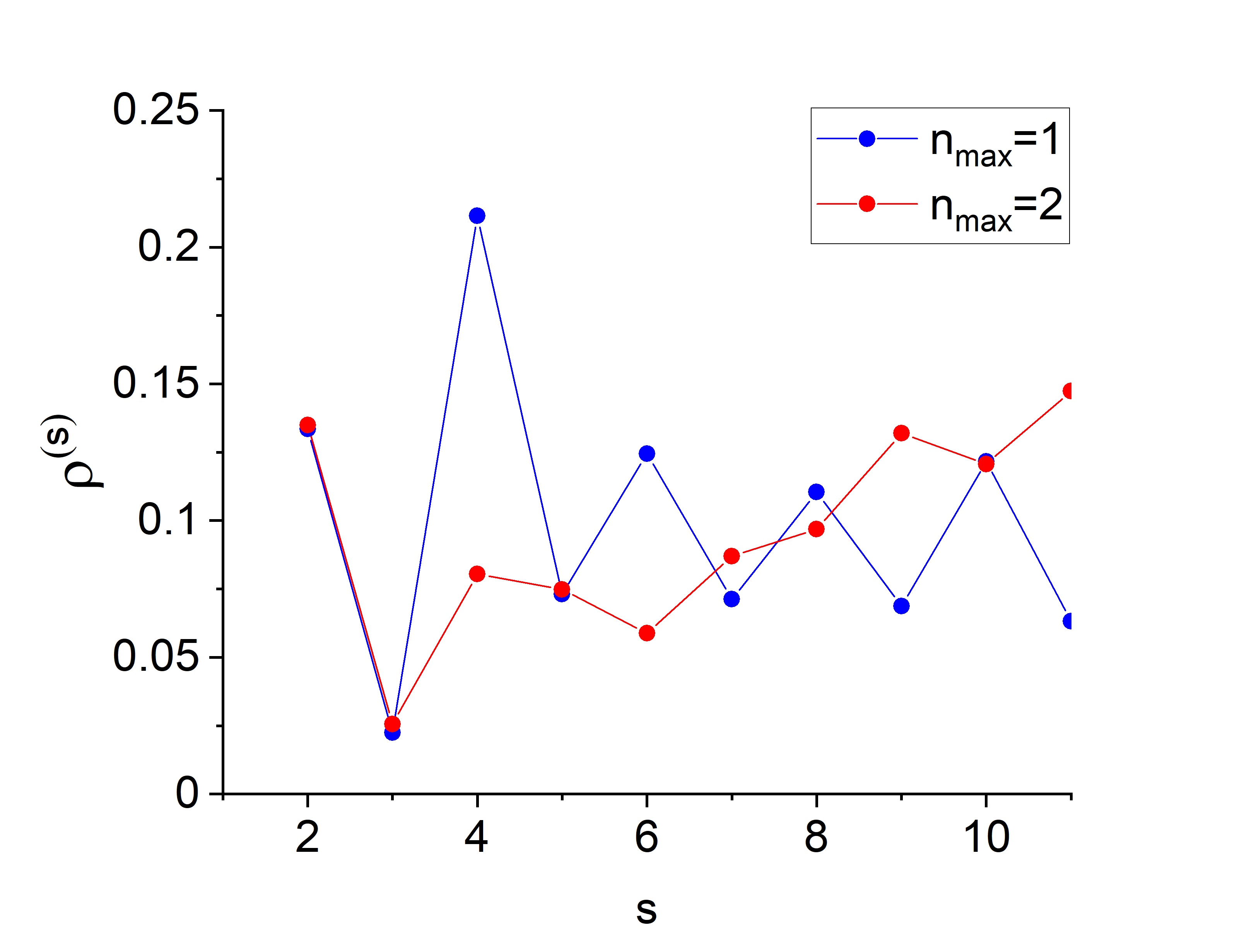
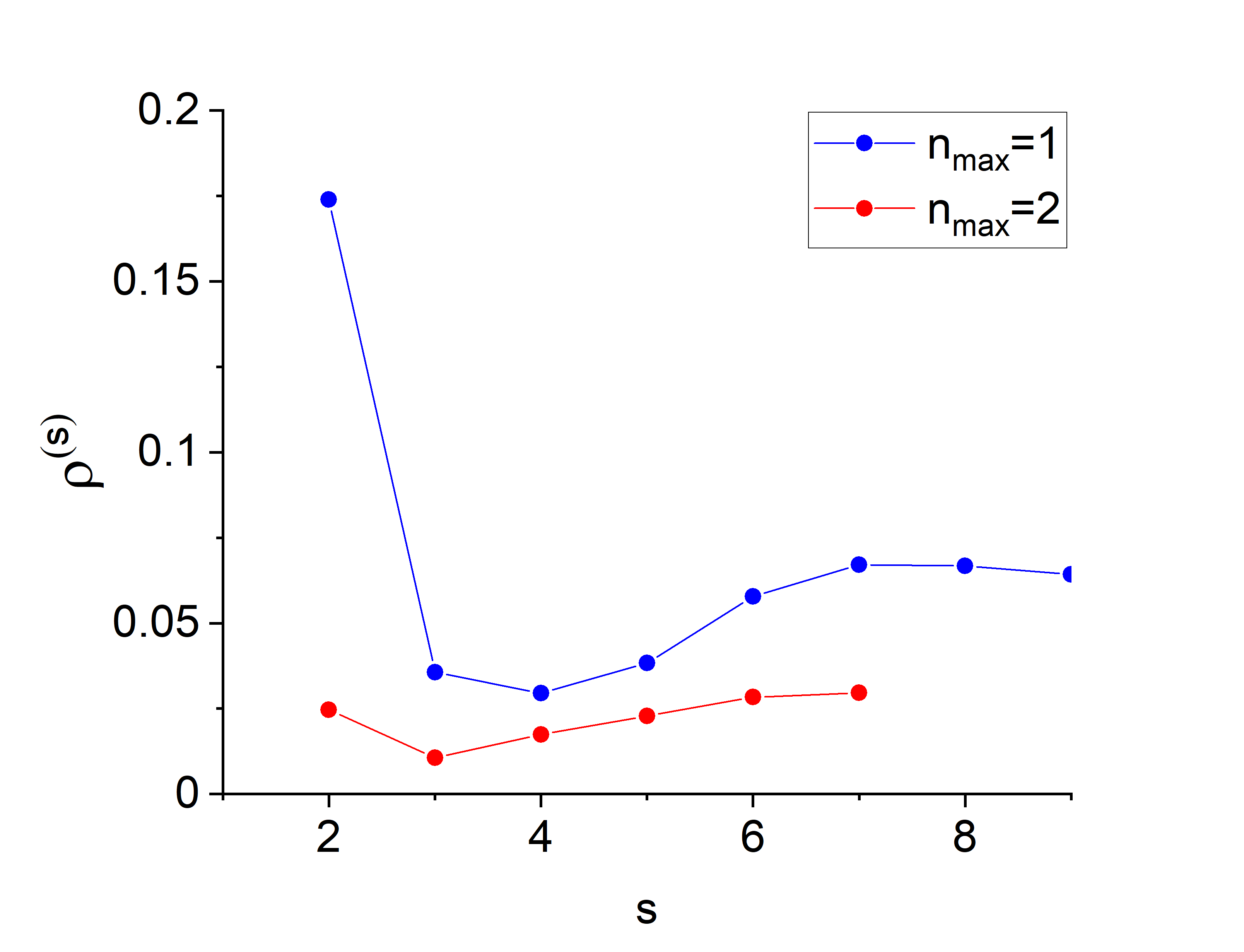
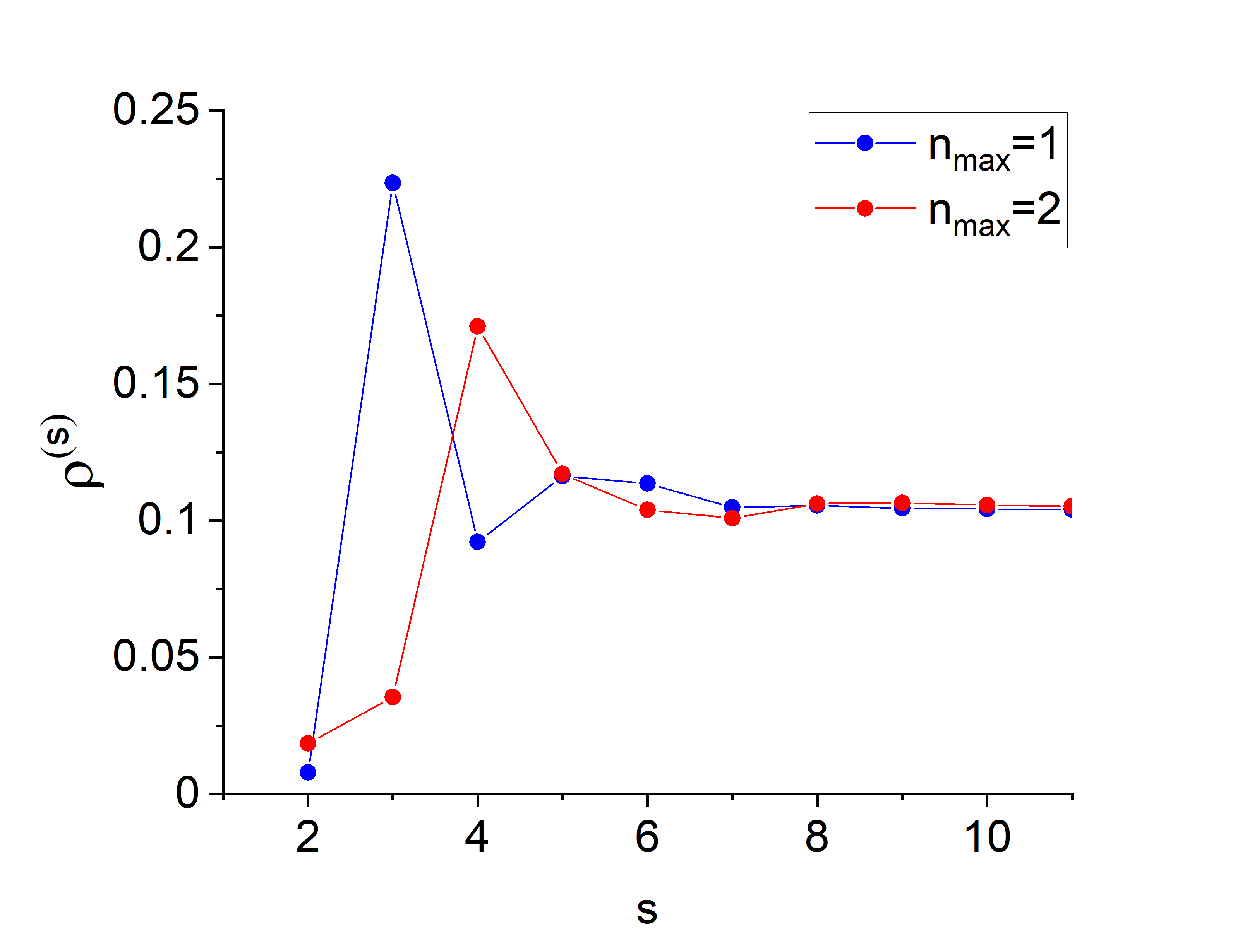
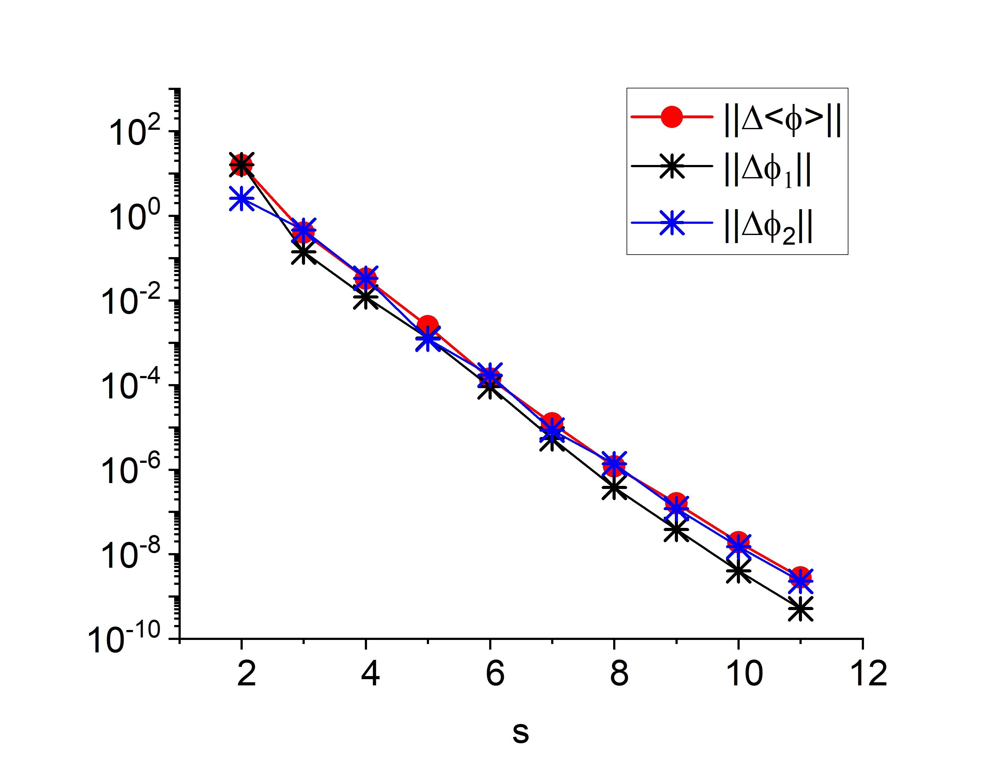
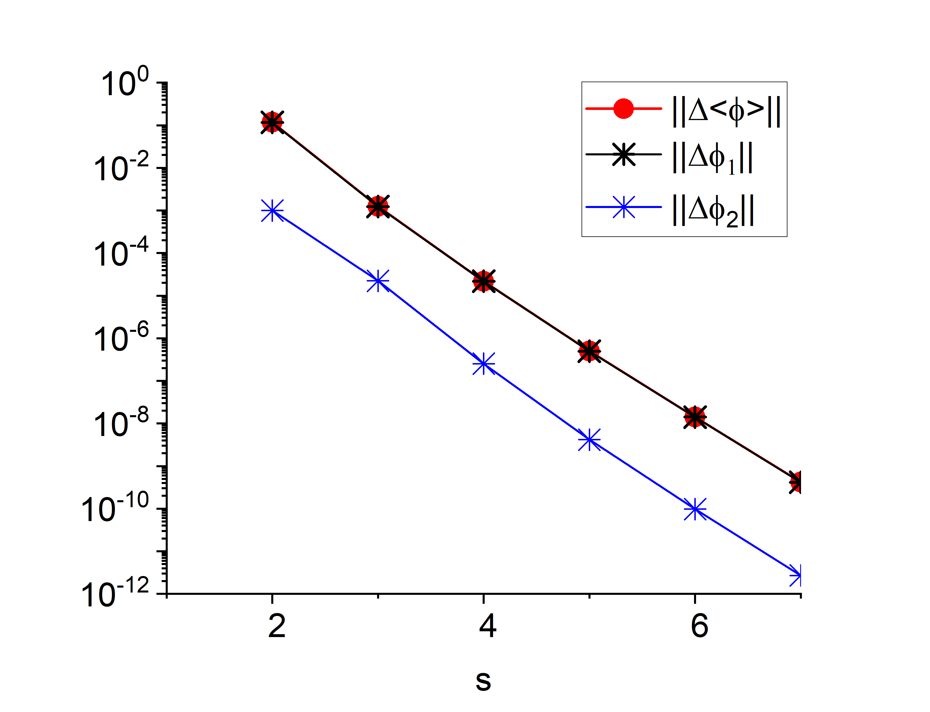
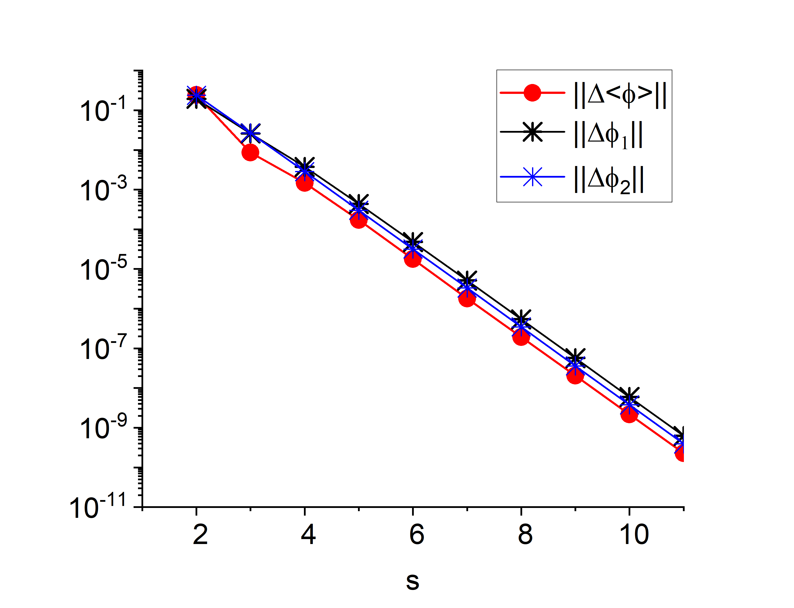
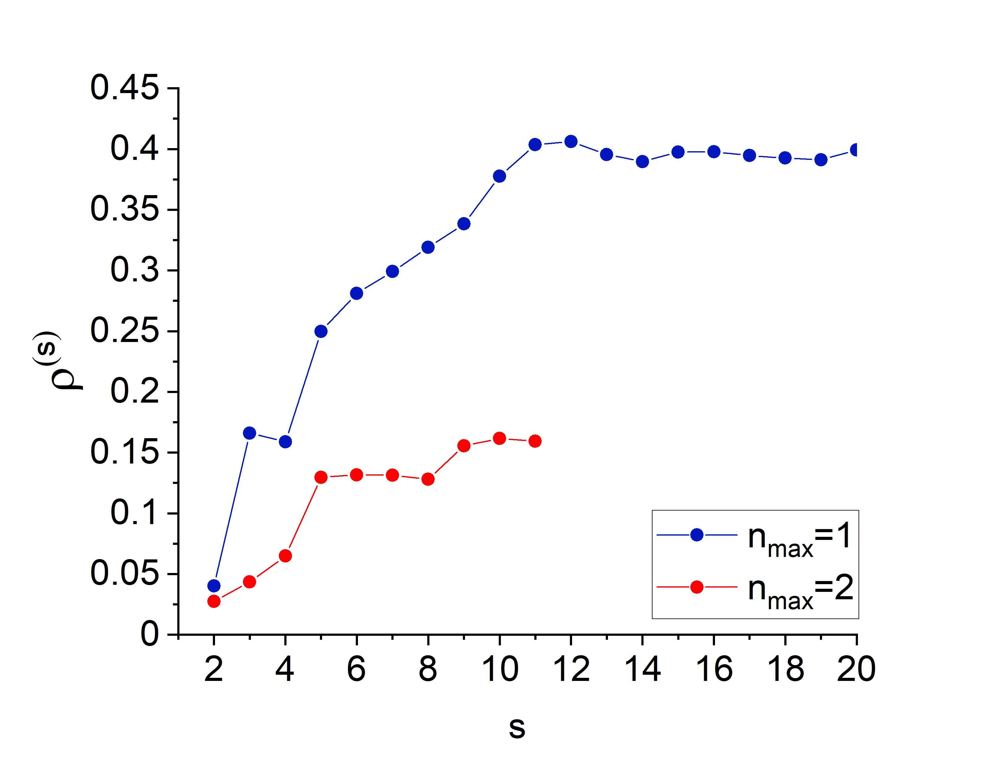
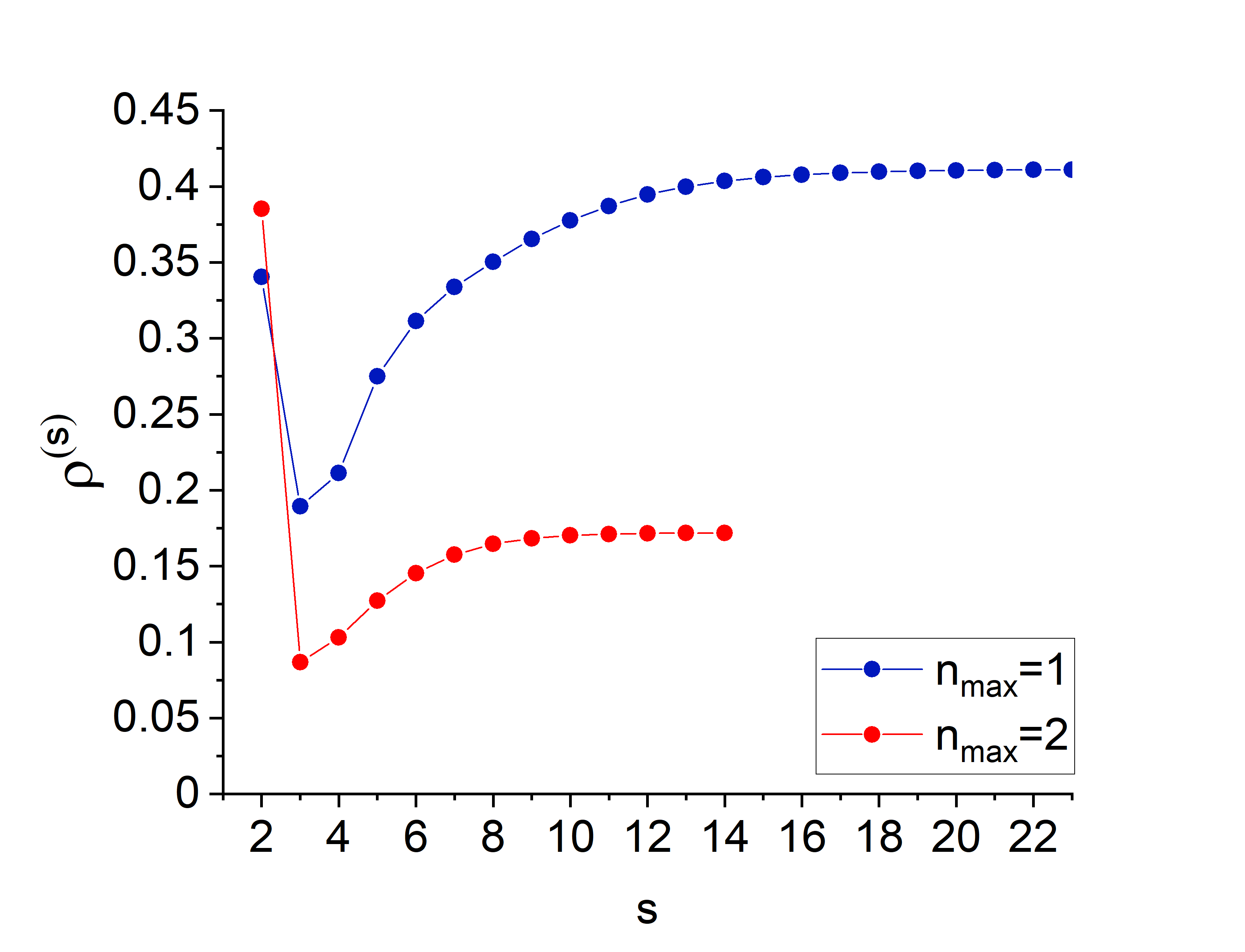
Table 2 presents numerically estimated spectral radii in every test. The results for algorithms with one and two GS inner iterations in the high-order transport problem ($n_{max}=1,2$) are shown. To demonstrate details of iterative behavior of the algorithms, Figures 3 and 5 show convergence rates of the total ensemble average scalar flux

$$\rho^{(s)}=\frac{\big{|}\big{|}\Delta\big{<}\phi\big{>}^{(s)}\big{|}\big{|}_{\infty}}{\big{|}\big{|}\Delta\big{<}\phi\big{>}^{(s-1)}\big{|}\big{|}_{\infty}}\,,\quad\Delta\big{<}\phi\big{>}^{(s)}=\big{<}\phi\big{>}^{(s)}-\big{<}\phi\big{>}^{(s-1)}\,$$ (28)

in Tests $A_{k}$ and $C_{k}$, respectively. The algorithm with two relaxation cycles in the high-order problem ($n_{max}=2$) converges fast in all tests. In Tests $A_{k}$ and $D_{k}$, the spectral radii of this algorithm are smaller than those of the algorithm with one relaxation cycle ($n_{max}=1$). In Tests $B_{k}$ and $C_{k}$, the algorithm with one relaxation cycle is rapidly converging. Performance of the algorithms with 1 and 2 relaxation cycles are close to each other in these two sets of tests.

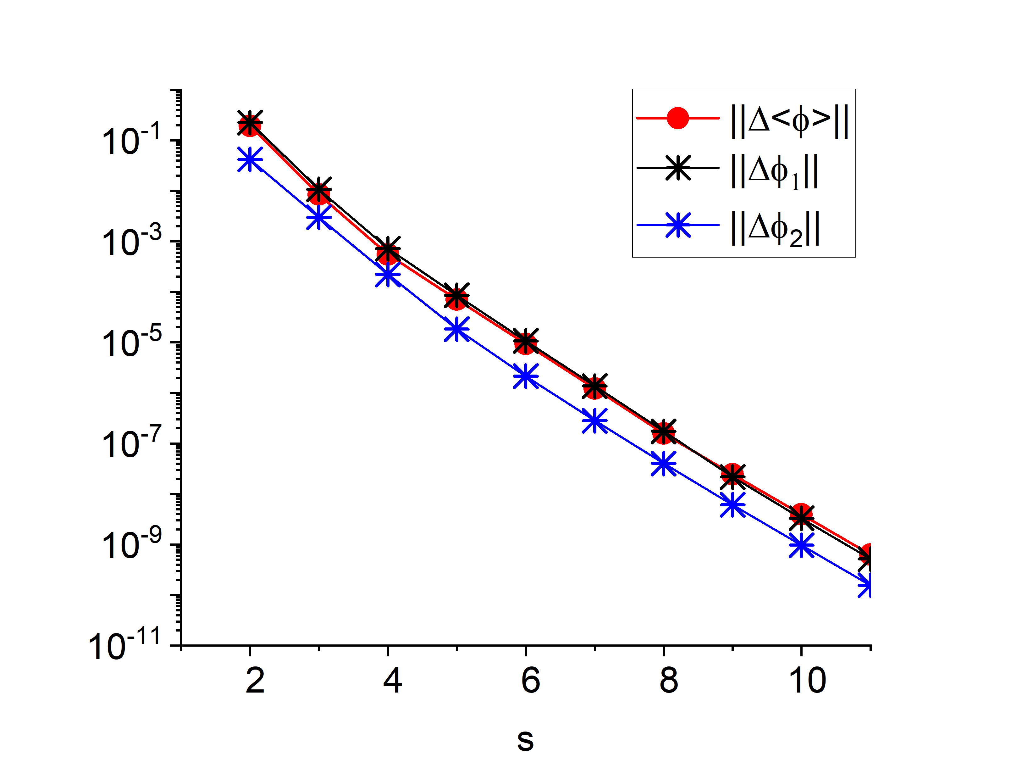
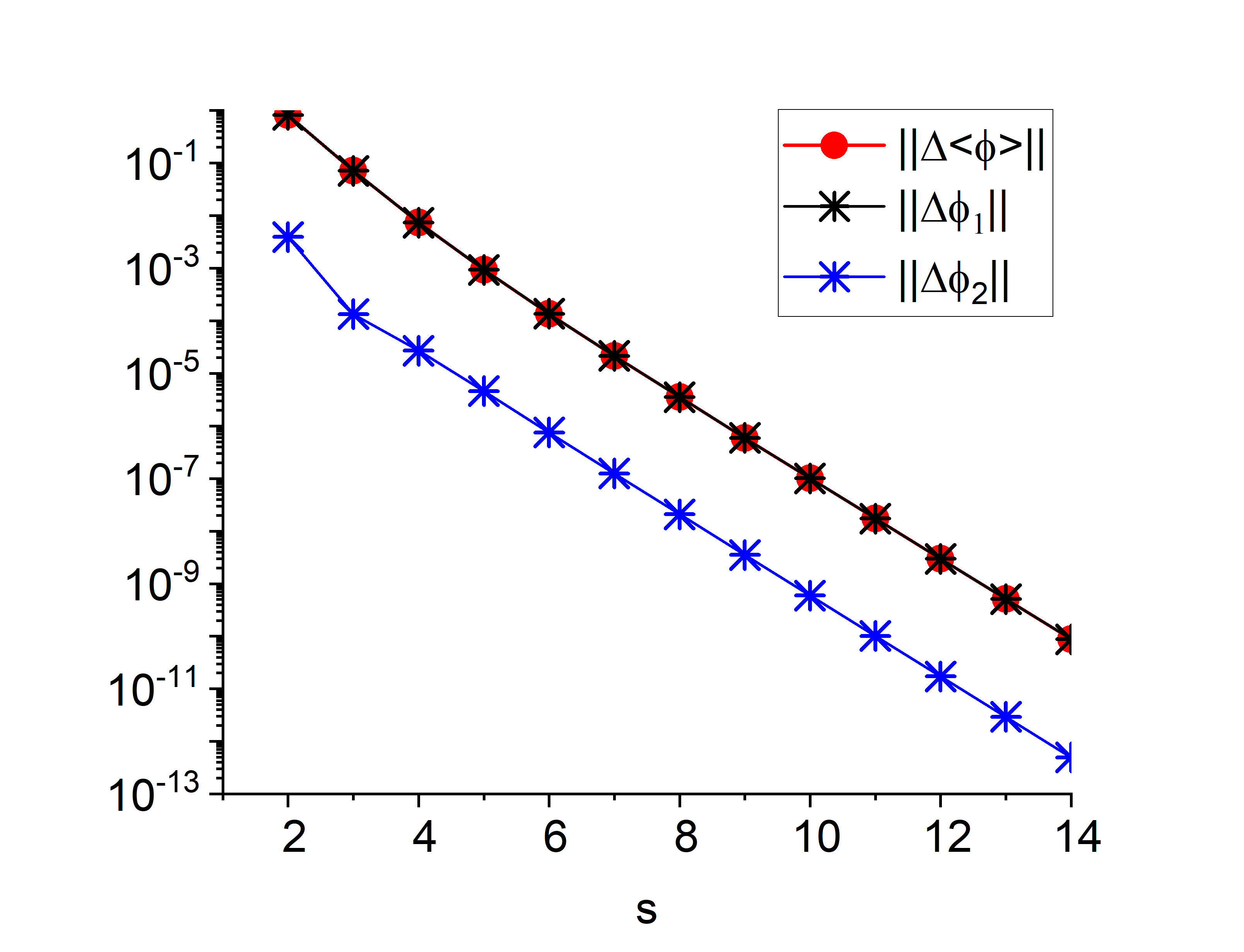
Figures 3 and 5 present convergence curves of $||\Delta\big{<}\phi\big{>}^{(s)}||_{\infty}$ and $||\Delta\phi_{\ell}^{(s)}||_{\infty}$ in Tests $A_{k}$ and $C_{k}$, where $\Delta\phi_{\ell}^{(s)}=\phi_{\ell}^{(s)}-\phi_{\ell}^{(s-1)}$. The CEA of the material scalar fluxes and total ensemble average of the scalar flux converge with close rates. The convergence behavior in other tests is similar.

(a) Test A₁

(b) Test A₂

(c) Test A₃

Figure 2: Convergence rates $\rho^{(s)}$ in Tests A_k

(a) Test A₁

(b) Test A₂

(c) Test A₃

Figure 3: Convergence curves of $\big{<}\phi\big{>}^{(s)}$ and $\phi_{\ell}^{(s)}$ in Tests A_k, $n_{max}=2$

(a) Test C₁

(b) Test C₂

(c) Test C₃

Figure 4: Convergence rates $\rho^{(s)}$ in Tests C_k

(a) Test C₁

(b) Test C₂

(c) Test C₃

Figure 5: Convergence curves of $\big{<}\phi\big{>}^{(s)}$ and $\phi_{\ell}^{(s)}$ in Tests C_k, $n_{max}=2$

5 Conclusions

A new iteration method for the transport equation in binary stochastic media has been presented. It is formulated by means of a hierarchy of equations consisting of the high-order transport equation for the CEA of the angular flux and the low-order equations for (i) the CEA of the material partial scalar fluxes and (ii) the total ensemble average scalar flux and current. The obtained results show that the multilevel method accelerates transport iterations in the considered class of test problems. Further analysis is needed to study efficiency of the iteration method. One of items is convergence in the atomic mix limit as $\lambda_{\ell}\sigma_{t,\ell}\to 0$.

There are various possible modifications that can be applied to the multilevel method, for example, Anderson acceleration, nonlinear Krylov acceleration and advanced prolongation operators for the CEA of the angular flux. The low-order equations of the multilevel method correspond to different scales of the physical problem. This method has a potential for nonlinear radiation transport problems in random media in which the transport equation is coupled with multiphysics equations.

References

• [1] C.Β D. Levermore, G.Β C. Pomraning, D.Β L. Sanzo, J.Β Wong, Linear transport theory in a random medium, Journal of Mathematical Physics 27 (1986) 2526–2536.
• [2] M. L. Adams, E. W. Larsen, G. C. Pomraning, Benchmark results for particle transport in a binary Markov statistical medium, Journal of Quantitative Spectroscopy Radiative Transfer 4 (1989) 253–266.
• [3] F. Malvagi, G. C. Pomraning, Renormalized equations for linear transport in stochastic media, J. Mathematical Physics 31 (1990) 892–900.
• [4] G.Β Pomraning, Linear Kinetic Theory and Particle Transport in Stochastic Mixtures, World Scientific, Singapore, New York, London, Hong Kong, 1991.
• [5] B.Β Ching, T.Β Palmer, Analysis of iterative schemes for binary stochastic mixture transport equations, Transactions of the American Nuclear Society 82 (2000) 148.
• [6] D. S. Miller, G. Rodrigue, F. Graziani, Convergence analysis of source iteration for the solution of coupled transport equations on a stochastic media, Transport Theory and Statistical Physics 31 (2002) 65–83.
• [7] G.B. Zimmerman, M. L. Adams, Algorithms for Monte Carlo particle transport in binary statistical mixtures, Transactions of the American Nuclear Society 63 (1991) 287–288.
• [8] A. K. Prinja, E. D. Fichtl, Atomic mix synthetic acceleration of dose computations in binary statistical media, Nuclear Science and Engineering 155 (2007) 441–448.
• [9] T. S. Palmer, B. S. Ching, A β€œtwo-grid’” acceleration of binary stochastic mixture deterministic transport iterations in slab geometry, Annals of Nuclear Energy 35 (2008) 68–74.
• [10] T. S. Palmer, A coupled diffusion synthetic acceleration for binary stochastic mixture transport iterations, Nuclear Science and Engineering 158 (2008) 40–48.
• [11] E.Β D. Fichtl, J.Β S. Warsa, A.Β K. Prinja, Krylov iterative methods and synthetic acceleration for transport in binary statistical media, Journal of Computational Physics 228 (2009) 8413–8426.
• [12] V.Β Y. Gol’din, On mathematical modeling of problems of non-equilibrium transfer in physical systems, in: Modern Problems of Mathematical Physics and Computational Mathematics, Nauka, Moscow, 1982, pp. 113–127, in Russian.
• [13] D.Β Y. Anistratov, V.Β Y. Gol’din, Nonlinear methods for solving particle transport problems, Transport Theory and Statistical Physics 22 (1993) 42–77.
• [14] D. S. Miller, G. Rodrigue, F. Graziani, Benchmarks and models for time-dependent grey radiation transport with material temperature in binary stochastic media, J. of Quantitative Spectroscopy & Radiative Transfer 70 (2001) 115–128.
• [15] D.Β Y. Anistratov, Stability analysis of a multilevel quasidiffusion method for thermal radiative transfer problems, J. of Computational Physics 376 (2019) 186–209.
• [16] J.Β J. Yvon, J. Nucl Energy 4 (1957) 305.
• [17] R.Β Mertens, Simon Stevin Supplement 30.
• [18] G.Β Bell, S.Β Glasstone, Nuclear Reactor Theory, Van Nostrand Reinhold Company, New York,Cincinnati, Toronto, London, Melbourne, 1970.
• [19] S. Santandrea, R. Sanchez, Analysis and improvements of the DPN acceleration technique for the method of characteristics in unstructured meshes, Annals of Nuclear Energy 32 (2005) 163–193.
• [20] S.Β S. Nikolaishvilli, On solution of one-velocity transport equation based on Yvon-Mertens approximation, Soviet Atomic Energy 20 (1966) 344.
• [21] V.Β Y. Gol’din, A quasi-diffusion method of solving the kinetic equation, USSR Computational Mathematics and Mathematical Physics. 4 (1964) 136–149.
• [22] D.Β Y. Anistratov, J.Β S. Warsa, Discontinuous finite element quasidiffusion methods, Nuclear Science and Engineering 191 (2018) 105–120.