Fast and accurate randomized algorithms for low-rank tensor decompositionsthanks: This work is supported by the US NSF OAC via award No. 1942995.

Linjian Ma
Department of Computer Science
University of Illinois at Urbana-Champaign
lma16@illinois.edu
   Edgar Solomonik
Department of Computer Science
University of Illinois at Urbana-Champaign
solomon2@illinois.edu
Abstract

Low-rank Tucker and CP tensor decompositions are powerful tools in data analytics. The widely used alternating least squares (ALS) method, which solves a sequence of over-determined least squares subproblems, is costly for large and sparse tensors. We propose a fast and accurate sketched ALS algorithm for Tucker decomposition, which solves a sequence of sketched rank-constrained linear least squares subproblems. Theoretical sketch size upper bounds are provided to achieve 𝒪(ϵ)𝒪italic-ϵ\mathcal{O}\left(\epsilon\right) relative error for each subproblem with two sketching techniques, TensorSketch and leverage score sampling. Experimental results show that this new ALS algorithm, combined with a new initialization scheme based on randomized range finder, yields up to 22.0%percent22.022.0\% relative decomposition residual improvement compared to the state-of-the-art sketched randomized algorithm for Tucker decomposition of various synthetic and real datasets. This Tucker-ALS algorithm is further used to accelerate CP decomposition, by using randomized Tucker compression followed by CP decomposition of the Tucker core tensor. Experimental results show that this algorithm not only converges faster, but also yields more accurate CP decompositions.

1 Introduction

Tensor decompositions [30] are general tools for compression and approximation of high dimensional data, and are widely used in both scientific computing [45, 24, 25] and machine learning [3, 47]. In this paper, we focus on Tucker decomposition [53] and CANDECOMP/PARAFAC (CP) decomposition [23, 22]. Both decompositions are higher order generalizations of the matrix singular value decomposition (SVD). Tucker decomposition decomposes the input tensor into a core tensor along with factor matrices composed of orthonormal columns. CP decomposition decomposes the input tensor into a sum of outer products of vectors, which may also be assembled into factor matrices.

The alternating least squares (ALS) method is most widely used to compute both CP and Tucker decompositions. The ALS algorithm consists of sweeps, and each sweep updates every factor matrix once in a fixed order. The ALS method for Tucker decomposition, called the higher-order orthogonal iteration (HOOI) [4, 15, 30], updates one of the factor matrices along with the core tensor at a time. Similarly, each update procedure in the ALS algorithm for CP decomposition (CP-ALS) updates one of the factor matrices. For both decompositions, each optimization subproblem guarantees decrease of the decomposition residual.

In this work, we consider decomposition of order N𝑁N tensors (𝓣𝓣\boldsymbol{\mathcal{T}}) that are large in dimension size (s𝑠s) and can be potentially sparse. We focus on the problem of computing low-rank (with target rank Rsmuch-less-than𝑅𝑠R\ll s and Rnnz(𝓣)much-less-than𝑅nnz𝓣R\ll\operatorname{nnz}(\boldsymbol{\mathcal{T}})) decompositions for such tensors via ALS, which is often used for extracting principal component information from large-scale datasets. For Tucker decomposition, ALS is bottlenecked by the operation called the tensor times matrix-chain (TTMc). For CP decomposition, ALS is bottlenecked by the operation called the matricized tensor-times Khatri-Rao product (MTTKRP). Both TTMc and MTTKRP have a per-sweep cost of Ω(nnz(𝓣)R)Ωnnz𝓣𝑅\Omega(\operatorname{nnz}(\boldsymbol{\mathcal{T}})R) [49]. Consequently, the per-sweep costs of both HOOI and CP-ALS are proportional to the number of nonzeros in the tensor, which are expensive for large tensors with billions of nonzeros.

Recent works have applied different randomized techniques to accelerate both CP and Tucker decompositions. Based on sketching techniques introduced for low-rank matrix approximation [55], several sketching algorithms have been developed for CP decomposition [31, 1, 13, 56]. These algorithms accelerate CP-ALS by approximating the original highly over-determined linear least squares problems by smaller sketched linear least squares problems. These techniques have been shown to greatly improve the efficiency compared to the original ALS. For Tucker decomposition, several randomized algorithms based on random projection [12, 2, 11, 38, 56, 52] have been developed to accelerate higher-order singular value decomposition (HOSVD) [14, 53]. However, these methods calculate the core tensor via TTMc among the input tensor and all the factor matrices, which incurs a cost of Ω(nnz(𝓣)R)Ωnnz𝓣𝑅\Omega(\operatorname{nnz}(\boldsymbol{\mathcal{T}})R) for sparse tensors.

Becker and Malik [37] introduced a sketched ALS algorithm for Tucker decomposition, which avoids the expensive cost of TTMc. Unlike the traditional HOOI, each sweep of this ALS scheme contains N+1𝑁1N+1 subproblems, where only one of the factor matrices or the core tensor is updated in each subproblem. This scheme is easier to analyze theoretically, since each subproblem is an unconstrained linear least squares problem, which can be efficiently solved via sketching. However, the scheme produces decompositions that are generally less effective than HOOI.

1.1 Our Contributions

In this work, we propose a new sketched ALS algorithm for Tucker decomposition. Different from Becker and Malik [37], our ALS scheme is the same as HOOI, where one of the factor matrices along with the core tensor are updated in each subproblem. This guarantees the algorithm can reach the same accuracy as HOOI with sufficient sketch size. Experimental results show that it provides more accurate results compared to those in [37].

In this scheme, each subproblem is a sketched rank-constrained linear least squares problem, with the left-hand-side matrix with size sN1×RN1superscript𝑠𝑁1superscript𝑅𝑁1s^{N-1}\times R^{N-1} composed of orthonormal columns. To the best of our knowledge, the relative error analysis of sketching techniques for this problem have not been discussed in the literature. Existing works either only provide sketch size upper bounds for the relaxed problem [46], where rank constraint is relaxed with a nuclear norm constraint, or provide upper bounds for general constrained problems, which are too loose [55]. We provide tighter sketch size upper bounds to achieve 𝒪(ϵ)𝒪italic-ϵ\mathcal{O}\left(\epsilon\right) relative error with two state-of-the-art sketching techniques, TensorSketch [43] and leverage score sampling [17].

With leverage score sampling, our analysis shows that with probability at least 1δ1𝛿1-\delta, the sketch size of 𝒪(RN1/(ϵ2δ))𝒪superscript𝑅𝑁1superscriptitalic-ϵ2𝛿\mathcal{O}\left(R^{N-1}/(\epsilon^{2}\delta)\right) is sufficient for results with 𝒪(ϵ)𝒪italic-ϵ\mathcal{O}\left(\epsilon\right)-relative error. With TensorSketch, the sketch size upper bound is 𝒪((RN13N1)/δ(RN1+1/ϵ2))𝒪superscript𝑅𝑁1superscript3𝑁1𝛿superscript𝑅𝑁11superscriptitalic-ϵ2\mathcal{O}\left((R^{N-1}\cdot 3^{N-1})/\delta\cdot(R^{N-1}+1/\epsilon^{2})\right), at least 𝒪(3N1)𝒪superscript3𝑁1\mathcal{O}\left(3^{N-1}\right) times that for leverage score sampling. For both techniques, our bounds are at most 𝒪(1/ϵ)𝒪1italic-ϵ\mathcal{O}\left(1/\epsilon\right) times the sketch size upper bounds for the unconstrained linear least squares problem.

The upper bounds suggest that under the same accuracy criteria, leverage score sampling potentially needs smaller sketch size for each linear least squares problem and thus can be more efficient than TensorSketch. Therefore, with the same sketch size, the accuracy with leverage score sampling can be better. However, with the standard random initializations for factor matrices, leverage score sampling can perform poorly on tensors with high coherence [9] (the orthogonal basis for the row space of each matricization of the input tensor has large row norm variability), making it less robust than TensorSketch. To improve the robustness of leverage score sampling, we introduce an algorithm that uses the randomized range finder (RRF) [21] to initialize the factor matrices. The initialization scheme uses the composition of CountSketch and Gaussian random matrix as the RRF embedding matrix, which only requires one pass over the non-zero elements of the input tensor. Our experimental results show that the leverage score sampling based randomized algorithm combined with this RRF scheme performs well on tensors with high coherence.

For Rsmuch-less-than𝑅𝑠R\ll s, our new sketching based algorithm for Tucker decomposition can also be used to accelerate CP decomposition. Tucker compression is performed first, and then CP decomposition is applied to the core tensor [56, 8, 19]. Since the per-sweep costs for both sketched Tucker-ALS and sketched CP-ALS are comparable, and Tucker-ALS often needs much fewer sweeps than CP-ALS (Tucker-ALS typically converges in less than 5 sweeps based on our experiments), this Tucker + CP method can be more efficient than directly applying randomized CP decomposition [31, 13] on the input tensor.

In summary, this paper makes the following contributions.

  • We introduce a new sketched ALS algorithm for Tucker decomposition, which contains a sequence of sketched rank-constrained linear least squares subproblems. We provide theoretical upper bounds for the sketch size, and experimental results show that the algorithm provides up to 22.0%percent22.022.0\% relative decomposition residual improvement compared to the previous work.

  • We provide detailed comparison of TensorSketch and leverage score sampling in terms of efficiency and accuracy. Our theoretical analysis shows that leverage score sampling is better in terms of both metrics.

  • We propose an initialization scheme based on RRF that improves the accuracy of leverage score sampling based sketching algorithm on tensors with high coherence.

  • We show that CP decomposition can be more efficiently and accurately calculated based on the sketched Tucker + CP method, compared to directly performing sketched CP-ALS on the input tensor.

1.2 Organization

Section 2 introduces notation used throughout the paper, ALS algorithms for Tucker and CP decompositions, and previous work. Section 3 introduces TensorSketch and leverage score sampling techniques. In Section 4, we provide sketch size upper bounds for the rank-constrained linear least squares subproblems in sketched Tucker-ALS. Detailed proofs are presented in Appendix A. In Section 5, we introduce the initialization scheme for factor matrices via randomized range finder. In Section 6, we present detailed cost analysis for our new sketched ALS algorithms. We present experimental results in Section 7 and conclude in Section 8.

2 Background

2.1 Notation

Our analysis makes use of tensor algebra in both element-wise equations and specialized notation for tensor operations [30]. Vectors are denoted with bold lowercase Roman letters (e.g., 𝐯𝐯\mathbf{v}), matrices are denoted with bold uppercase Roman letters (e.g., 𝐌𝐌\mathbf{M}), and tensors are denoted with bold calligraphic font (e.g., 𝓣𝓣\boldsymbol{\mathcal{T}}). An order N𝑁N tensor corresponds to an N𝑁N-dimensional array. Elements of vectors, matrices, and tensors are denoted in parentheses, e.g., 𝐯(i)𝐯𝑖\mathbf{v}(i) for a vector 𝐯𝐯\mathbf{v}, 𝐌(i,j)𝐌𝑖𝑗\mathbf{M}(i,j) for a matrix 𝐌𝐌\mathbf{M}, and 𝓣(i,j,k,l)𝓣𝑖𝑗𝑘𝑙\boldsymbol{\mathcal{T}}(i,j,k,l) for an order 4 tensor 𝓣𝓣\boldsymbol{\mathcal{T}}. The i𝑖ith column of 𝐌𝐌\mathbf{M} is denoted by 𝐌(:,i)𝐌:𝑖\mathbf{M}(:,i), and the i𝑖ith row is denoted by 𝐌(i,:)𝐌𝑖:\mathbf{M}(i,:). Parenthesized superscripts are used to label different vectors, matrices and tensors (e.g. 𝓣(1)superscript𝓣1\boldsymbol{\mathcal{T}}^{(1)} and 𝓣(2)superscript𝓣2\boldsymbol{\mathcal{T}}^{(2)} are unrelated tensors). Number of nonzeros of the tensor 𝓣𝓣\boldsymbol{\mathcal{T}} is denoted by nnz(𝓣)nnz𝓣\operatorname{nnz}(\boldsymbol{\mathcal{T}}).

The pseudo-inverse of matrix 𝐀𝐀\mathbf{A} is denoted with 𝐀superscript𝐀\mathbf{A}^{\dagger}. The Hadamard product of two matrices is denoted with *. The outer product of two or more vectors is denoted with \circ. The Kronecker product of two vectors/matrices is denoted with tensor-product\otimes. For matrices 𝐀m×k𝐀superscript𝑚𝑘\mathbf{A}\in\mathbb{R}^{m\times k} and 𝐁n×k𝐁superscript𝑛𝑘\mathbf{B}\in\mathbb{R}^{n\times k}, their Khatri-Rao product results in a matrix of size (mn)×k𝑚𝑛𝑘(mn)\times k defined by 𝐀𝐁=[𝐀(:,1)𝐁(:,1),,𝐀(:,k)𝐁(:,k)].direct-product𝐀𝐁tensor-product𝐀:1𝐁:1tensor-product𝐀:𝑘𝐁:𝑘\mathbf{A}\odot\mathbf{B}=[\mathbf{A}(:,1)\otimes\mathbf{B}(:,1),\ldots,\mathbf{A}(:,k)\otimes\mathbf{B}(:,k)]. The mode-n𝑛n tensor times matrix of an order N𝑁N tensor 𝓣s1××sN𝓣superscriptsubscript𝑠1subscript𝑠𝑁\boldsymbol{\mathcal{T}}\in\mathbb{R}^{s_{1}\times\cdots\times s_{N}} with a matrix AJ×snAsuperscript𝐽subscript𝑠𝑛\textbf{A}\in\mathbb{R}^{J\times s_{n}} is denoted by 𝓣×n𝐀subscript𝑛𝓣𝐀\boldsymbol{\mathcal{T}}\times_{n}\mathbf{A}, whose output size is s1××sn1×J×sn+1××sNsubscript𝑠1subscript𝑠𝑛1𝐽subscript𝑠𝑛1subscript𝑠𝑁s_{1}\times\cdots\times s_{n-1}\times J\times s_{n+1}\times\cdots\times s_{N}. Matricization is the process of unfolding a tensor into a matrix. The mode-n𝑛n matricized version of 𝓣𝓣\boldsymbol{\mathcal{T}} is denoted by T(n)sn×KsubscriptT𝑛superscriptsubscript𝑠𝑛𝐾\textbf{T}_{(n)}\in\mathbb{R}^{s_{n}\times K} where K=m=1,mnNsm𝐾superscriptsubscriptproductformulae-sequence𝑚1𝑚𝑛𝑁subscript𝑠𝑚K=\prod_{m=1,m\neq n}^{N}s_{m}. We use [N]delimited-[]𝑁[N] to denote {1,,N}1𝑁\{1,\ldots,N\}. 𝒪~~𝒪\widetilde{\mathcal{O}} denotes the asymptotic cost with logarithmic factors ignored.

2.2 Tucker Decomposition with ALS

We review the ALS method for computing Tucker decomposition of an input tensor [53]. Throughout the analysis we assume the input tensor has order N𝑁N and size s××s𝑠𝑠s\times\cdots\times s, and the Tucker ranks are R××R𝑅𝑅R\times\cdots\times R. Tucker decomposition approximates a tensor by a core tensor contracted along each mode with matrices that have orthonormal columns. The goal of Tucker decomposition is to minimize the objective function,

f(𝓒,𝐀(1),,𝐀(N)):=12𝓣𝓒×1𝐀(1)×2𝐀(2)×N𝐀(N)F2.assign𝑓𝓒superscript𝐀1superscript𝐀𝑁12superscriptsubscriptnorm𝓣subscript𝑁subscript2subscript1𝓒superscript𝐀1superscript𝐀2superscript𝐀𝑁𝐹2f(\boldsymbol{\mathcal{C}},\mathbf{A}^{(1)},\ldots,\mathbf{A}^{(N)}):=\frac{1}{2}\left\|\boldsymbol{\mathcal{T}}-\boldsymbol{\mathcal{C}}\times_{1}\mathbf{A}^{(1)}\times_{2}\mathbf{A}^{(2)}\cdots\times_{N}\mathbf{A}^{(N)}\right\|_{F}^{2}. (2.1)

The core tensor 𝓒𝓒\boldsymbol{\mathcal{C}} is of order N𝑁N with dimensions R××R𝑅𝑅R\times\cdots\times R. Each matrix A(n)s×RsuperscriptA𝑛superscript𝑠𝑅\textbf{A}^{(n)}\in\mathbb{R}^{s\times R} for n[N]𝑛delimited-[]𝑁n\in[N] has orthonormal columns. The ALS method for Tucker decomposition [4, 15, 30], called the higher-order orthogonal iteration (HOOI), proceeds by updating one of the factor matrices along with the core tensor at a time. The n𝑛nth subproblem can be written as

min𝓒,𝐀(n)12𝐏(n)𝐂(n)T𝐀(n)T𝐓(n)TF2,subscript𝓒superscript𝐀𝑛12superscriptsubscriptnormsuperscript𝐏𝑛superscriptsubscript𝐂𝑛𝑇superscript𝐀𝑛𝑇superscriptsubscript𝐓𝑛𝑇𝐹2\min_{\boldsymbol{\mathcal{C}},\mathbf{A}^{(n)}}\frac{1}{2}\left\|\mathbf{P}^{(n)}\mathbf{C}_{(n)}^{T}\mathbf{A}^{(n)T}-\mathbf{T}_{(n)}^{T}\right\|_{F}^{2}, (2.2)

where 𝐏(n)=𝐀(1)𝐀(n1)𝐀(n+1)𝐀(N)superscript𝐏𝑛tensor-productsuperscript𝐀1superscript𝐀𝑛1superscript𝐀𝑛1superscript𝐀𝑁\mathbf{P}^{(n)}=\mathbf{A}^{(1)}\otimes\cdots\otimes\mathbf{A}^{(n-1)}\otimes\mathbf{A}^{(n+1)}\otimes\cdots\otimes\mathbf{A}^{(N)}. This problem can be formulated as a rank-constrained linear least squares problem,

min𝐁(n)12𝐏(n)𝐁(n)𝐓(n)TF2,such thatrank(𝐁(n))R.subscriptsuperscript𝐁𝑛12superscriptsubscriptnormsuperscript𝐏𝑛superscript𝐁𝑛superscriptsubscript𝐓𝑛𝑇𝐹2such thatranksuperscript𝐁𝑛𝑅\min_{\mathbf{B}^{(n)}}\frac{1}{2}\left\|\mathbf{P}^{(n)}\mathbf{B}^{(n)}-\mathbf{T}_{(n)}^{T}\right\|_{F}^{2},\quad\text{such that}\quad\text{rank}(\mathbf{B}^{(n)})\leq R. (2.3)

𝐀(n)superscript𝐀𝑛\mathbf{A}^{(n)} corresponds to the right singular vectors of the optimal 𝐁(n)superscript𝐁𝑛\mathbf{B}^{(n)}, while 𝐂(n)T=𝐁(n)𝐀(n)superscriptsubscript𝐂𝑛𝑇superscript𝐁𝑛superscript𝐀𝑛\mathbf{C}_{(n)}^{T}=\mathbf{B}^{(n)}\mathbf{A}^{(n)}. Since 𝐏(n)superscript𝐏𝑛\mathbf{P}^{(n)} contains orthonormal columns, the optimal 𝐁(n)superscript𝐁𝑛\mathbf{B}^{(n)} can be obtained by calculating the Tensor Times Matrix-chain (TTMc),

𝓨(n)=𝓣×1𝐀(1)T×n1𝐀(n1)T×n+1𝐀(n+1)T×N𝐀(N)T,superscript𝓨𝑛subscript𝑁subscript𝑛1subscript𝑛1subscript1𝓣superscript𝐀1𝑇superscript𝐀𝑛1𝑇superscript𝐀𝑛1𝑇superscript𝐀𝑁𝑇\boldsymbol{\mathcal{Y}}^{(n)}=\boldsymbol{\mathcal{T}}\times_{1}\mathbf{A}^{(1)T}\cdots\times_{n-1}\mathbf{A}^{(n-1)T}\times_{n+1}\mathbf{A}^{(n+1)T}\cdots\times_{N}\mathbf{A}^{(N)T}, (2.4)

and taking 𝐁(n)superscript𝐁𝑛\mathbf{B}^{(n)} to be the transpose of the mode-n𝑛n matricized 𝓨(n)superscript𝓨𝑛\boldsymbol{\mathcal{Y}}^{(n)}, 𝐘(n)(n)Tsuperscriptsubscript𝐘𝑛𝑛𝑇\mathbf{Y}_{(n)}^{(n)T}. Calculating 𝓨(n)superscript𝓨𝑛\boldsymbol{\mathcal{Y}}^{(n)} costs 𝒪(sNR)𝒪superscript𝑠𝑁𝑅\mathcal{O}\left(s^{N}R\right) for dense tensors and 𝒪(nnz(𝓣)RN1)𝒪nnz𝓣superscript𝑅𝑁1\mathcal{O}\left(\operatorname{nnz}(\boldsymbol{\mathcal{T}})R^{N-1}\right) for sparse tensors. HOOI typically converges in less than 5 sweeps. Before the HOOI procedure, the factor matrices are often initialized with the higher-order singular value decomposition (HOSVD) [14, 53]. HOSVD computes the truncated SVD of each 𝐓(n)𝐔(n)𝚺(n)𝐕(n)Tsubscript𝐓𝑛superscript𝐔𝑛superscript𝚺𝑛superscript𝐕𝑛𝑇\mathbf{T}_{(n)}\approx\mathbf{U}^{(n)}\mathbf{\Sigma}^{(n)}\mathbf{V}^{(n)T}, and sets 𝐀(n)=𝐔(n)superscript𝐀𝑛superscript𝐔𝑛\mathbf{A}^{(n)}=\mathbf{U}^{(n)} for n[N]𝑛delimited-[]𝑁n\in[N]. If performing SVD via randomized SVD [21], updating 𝐀(n)superscript𝐀𝑛\mathbf{A}^{(n)} for each mode costs 𝒪(sNR)𝒪superscript𝑠𝑁𝑅\mathcal{O}\left(s^{N}R\right) for dense tensors, and costs 𝒪(sN1R2+nnz(𝓣)R)𝒪superscript𝑠𝑁1superscript𝑅2nnz𝓣𝑅\mathcal{O}\left(s^{N-1}R^{2}+\operatorname{nnz}(\boldsymbol{\mathcal{T}})R\right) for sparse tensors. The Tucker-ALS algorithm is presented in Algorithm 1.

Algorithm 1 Tucker-ALS: ALS procedure for Tucker decomposition
1:  Input: Tensor 𝓣s1××sN𝓣superscriptsubscript𝑠1subscript𝑠𝑁\boldsymbol{\mathcal{T}}\in\mathbb{R}^{s_{1}\times\cdots\times s_{N}}, decomposition ranks {R1,,RN}subscript𝑅1subscript𝑅𝑁\{R_{1},\ldots,R_{N}\}
2:  Initialize {𝐀(1),,𝐀(N)}superscript𝐀1superscript𝐀𝑁\{\mathbf{A}^{(1)},\ldots,\mathbf{A}^{(N)}\} using HOSVD
3:  while not converged do
4:     for n[N]𝑛delimited-[]𝑁n\in[N] do
5:        Update 𝓨(n)superscript𝓨𝑛\boldsymbol{\mathcal{Y}}^{(n)} based on (2.4)
6:        A(n)RnsuperscriptA𝑛subscript𝑅𝑛\textbf{A}^{(n)}\leftarrow R_{n} leading left singular vectors of Y(n)(n)subscriptsuperscriptY𝑛𝑛\textbf{Y}^{(n)}_{(n)}
7:     end for
8:     𝓒𝓨(N)×N𝐀(N)T𝓒subscript𝑁superscript𝓨𝑁superscript𝐀𝑁𝑇\boldsymbol{\mathcal{C}}\leftarrow\boldsymbol{\mathcal{Y}}^{(N)}\times_{N}\mathbf{A}^{(N)T}
9:  end while
10:  return  {𝓒,𝐀(1),,𝐀(N)}𝓒superscript𝐀1superscript𝐀𝑁\{\boldsymbol{\mathcal{C}},\mathbf{A}^{(1)},\ldots,\mathbf{A}^{(N)}\}

2.3 CP Decomposition with ALS

CP tensor decomposition [23, 22] decomposes the input tensor into a sum of outer products of vectors. Throughout analysis we assume the input tensor has order N𝑁N and size s××s𝑠𝑠s\times\cdots\times s, and the CP rank is R𝑅R. The goal of CP decomposition is to minimize the objective function,

f(𝐀(1),,𝐀(N)):=12𝓣r=1R𝐀(1)(:,r)𝐀(N)(:,r)F2,assign𝑓superscript𝐀1superscript𝐀𝑁12superscriptsubscriptnorm𝓣superscriptsubscript𝑟1𝑅superscript𝐀1:𝑟superscript𝐀𝑁:𝑟𝐹2f(\mathbf{A}^{(1)},\ldots,\mathbf{A}^{(N)}):=\frac{1}{2}\left\|\boldsymbol{\mathcal{T}}-\sum_{r=1}^{R}\mathbf{A}^{(1)}(:,r)\circ\cdots\circ\mathbf{A}^{(N)}(:,r)\right\|_{F}^{2}, (2.5)

where 𝐀(i)s×Rsuperscript𝐀𝑖superscript𝑠𝑅\mathbf{A}^{(i)}\in\mathbb{R}^{s\times R} for i[N]𝑖delimited-[]𝑁i\in[N] are called factor matrices. CP-ALS is the mostly widely used algorithm to get the factor matrices. In each ALS sweep, we solve N𝑁N subproblems, and the objective for the update of 𝐀(n)superscript𝐀𝑛\mathbf{A}^{(n)}, with n[N]𝑛delimited-[]𝑁n\in[N], is expressed as,

𝐀(n)=argmin𝐀12𝐏(n)𝐀T𝐗(n)TF2,\mathbf{A}^{(n)}=\arg\min_{\mathbf{A}}\frac{1}{2}\left\|\mathbf{P}^{(n)}\mathbf{A}{}^{T}-\mathbf{X}_{(n)}^{T}\right\|^{2}_{F}, (2.6)

where 𝐏(n)=𝐀(1)𝐀(n1)𝐀(n+1)𝐀(N).superscript𝐏𝑛direct-productsuperscript𝐀1superscript𝐀𝑛1superscript𝐀𝑛1superscript𝐀𝑁\mathbf{P}^{(n)}=\mathbf{A}^{(1)}\odot\cdots\odot\mathbf{A}^{(n-1)}\odot\mathbf{A}^{(n+1)}\odot\cdots\odot\mathbf{A}^{(N)}. Solving the linear least squares problem above has a cost of 𝒪(sNR)𝒪superscript𝑠𝑁𝑅\mathcal{O}\left(s^{N}R\right). For instance, when solving via normal equations the term 𝐏(n)T𝐗(n)Tsuperscript𝐏𝑛𝑇superscriptsubscript𝐗𝑛𝑇\mathbf{P}^{(n)T}\mathbf{X}_{(n)}^{T}, which is called MTTKRP, needs to be calculated, and it costs 𝒪(sNR)𝒪superscript𝑠𝑁𝑅\mathcal{O}\left(s^{N}R\right) for dense tensors and 𝒪(nnz(𝓣)R)𝒪nnz𝓣𝑅\mathcal{O}\left(\operatorname{nnz}(\boldsymbol{\mathcal{T}})R\right) for sparse tensors. We show the CP-ALS algorithm in Algorithm 2.

A major disadvantage of CP-ALS is its slow convergence. There are many cases where CP-ALS takes a large number of sweeps to converge when high resolution is necessary [40]. When R<s𝑅𝑠R<s, the procedure can be accelerated by performing Tucker-ALS first, which typically converges in fewer sweeps, and then computing a CP decomposition of the core tensor [10, 56, 8], which only has 𝒪(RN)𝒪superscript𝑅𝑁\mathcal{O}\left(R^{N}\right) elements.

Algorithm 2 CP-ALS: ALS procedure for CP decomposition
1:  Input: Tensor 𝓣s1××sN𝓣superscriptsubscript𝑠1subscript𝑠𝑁\boldsymbol{\mathcal{T}}\in\mathbb{R}^{s_{1}\times\cdots\times s_{N}}, rank R𝑅R
2:  Initialize {A(1),,A(N)}superscriptA1superscriptA𝑁\{\textbf{A}^{(1)},\ldots,\textbf{A}^{(N)}\} as uniformly distributed random matrices within [0,1]01[0,1]
3:  while not converged do
4:     for n[N]𝑛delimited-[]𝑁n\in[N] do
5:        Update 𝐀(n)superscript𝐀𝑛\mathbf{A}^{(n)} via solving Eq. 2.6
6:     end for
7:  end while
8:  return  {A(1),,A(N)}superscriptA1superscriptA𝑁\{\textbf{A}^{(1)},\ldots,\textbf{A}^{(N)}\}

2.4 Previous Work

Randomized algorithms have been applied to both Tucker and CP decompositions in several previous works. For Tucker decomposition, Ahmadi-Asl et al. [2] review a variety of random projection, sampling and sketching based randomized algorithms. Methods introduced in [12, 12, 11, 56, 52] accelerate the traditional HOSVD/HOOI via random projection, where factor matrices are updated based on performing SVD on the matricization of the randomly projected input tensor. For these methods, random projections are all performed based on Gaussian embedding matrices, and the core tensor is calculated via TTMc among the input tensor and all the factor matrices, which costs Ω(nnz(𝓣)R)Ωnnz𝓣𝑅\Omega(\operatorname{nnz}(\boldsymbol{\mathcal{T}})R) and is computationally inefficient for large sparse tensors. Sun et al. [51] introduce randomized algorithms for Tucker decompositions for streaming data.

The most similar work to ours is Becker and Malik [37]. This work computes Tucker decomposition via a sketched ALS scheme where in each optimization subproblem, one of the factor matrices or the core tensor is updated. They also solve each sketched linear least squares subproblem via TensorSketch. Our new scheme provides more accurate results compared to this method. Another work that is closely relevant to us is [38]. This work introduces structure-preserving decomposition, which is similar to Tucker decomposition but the factor matrices are not necessary orthogonal, and the entries of the core tensor are explicitly taken from the original tensor. The authors design an algorithm based on rank-revealing QR [20], which is efficient for sparse tensors, to calculate the decomposition. However, their experimental results show that the relative error of the algorithm for sparse tensors is much worse than that of the traditional HOSVD [38].

Several works discuss algorithms for sparse Tucker decomposition. Oh et al. [42] propose PTucker, which provides algorithms for scalable sparse Tucker decomposition. Kaya and Ucar [28] provide parallel algorithms for sparse Tucker decompositions. Li et al. [32] introduce SGD-Tucker, which uses stochastic gradient descent to perform Tucker decomposition of sparse tensors.

For CP decomposition, Battaglino et al. [6] and Jin et al. [26] introduce a randomized algorithm based on Kronecker fast Johnson-Lindenstrauss Transform (KFJLT) to accelerate CP-ALS. However, KFJLT is effective only for the decomposition of dense tensors. Aggour et al. [1] introduce adaptive sketching for CP decomposition. Song et al. [50] discuss the theoretical relative error of various tensor decompositions based on sketching. The work by Cheng et al. [13] and Larsen and Kolda [31] accelerate CP-ALS based on leverage score sampling. Cheng et al. [13] use leverage score sampling to accelerate MTTKRP calculations. Larsen and Kolda [31] propose an approximate leverage score sampling scheme for the Khatri-Rao product, and they show with 𝒪(R(N1)log(1/δ)/ϵ2)𝒪superscript𝑅𝑁11𝛿superscriptitalic-ϵ2\mathcal{O}\left(R^{(N-1)}\log(1/\delta)/\epsilon^{2}\right) number of samples, each unconstrained linear least squares subproblem in CP-ALS can be solved with 𝒪(ϵ)𝒪italic-ϵ\mathcal{O}\left(\epsilon\right)-relative error with probability at least 1δ1𝛿1-\delta. Zhou et al. [56] and Erichson et al. [19] accelerate CP decomposition via performing randomized Tucker decomposition of the input tensor first, and then performing CP decomposition of the smaller core tensor.

Several other works discuss techniques to parallelize and accelerate CP-ALS. Ma and Solomonik [34, 35] approximate MTTKRP within CP-ALS based on information from previous sweeps. For sparse tensors, parallelization strategies for MTTKRP have been developed both on shared memory systems [41, 49] and distributed memory systems [33, 48, 29].

3 Background on Sketching

Throughout the paper we consider the linear least squares problem,

min𝐗𝒞12𝐏𝐗𝐁F2,subscript𝐗𝒞12superscriptsubscriptnorm𝐏𝐗𝐁𝐹2\min_{\mathbf{X}\in\mathcal{C}}\frac{1}{2}\left\|\mathbf{P}\mathbf{X}-\mathbf{B}\right\|_{F}^{2}, (3.1)

where 𝐏=𝐀(1)𝐀(N)sN×RN𝐏tensor-productsuperscript𝐀1superscript𝐀𝑁superscriptsuperscript𝑠𝑁superscript𝑅𝑁\mathbf{P}=\mathbf{A}^{(1)}\otimes\cdots\otimes\mathbf{A}^{(N)}\in\mathbb{R}^{s^{N}\times R^{N}} is a chain of Kronecker products, N2𝑁2N\geq 2, 𝐏𝐏\mathbf{P} is dense and 𝐁𝐁\mathbf{B} is sparse. In each subproblem of Tucker HOOI, the feasible region 𝒞𝒞\mathcal{C} contains matrices with the rank constraint, as is shown in (2.3). The associated sketched problem is

min𝐗𝒞12𝐒𝐏𝐗𝐒𝐁F2,subscript𝐗𝒞12superscriptsubscriptnorm𝐒𝐏𝐗𝐒𝐁𝐹2\min_{\mathbf{X}\in\mathcal{C}}\frac{1}{2}\left\|\mathbf{S}\mathbf{P}\mathbf{X}-\mathbf{S}\mathbf{B}\right\|_{F}^{2}, (3.2)

where 𝐒m×sN𝐒superscript𝑚superscript𝑠𝑁\mathbf{S}\in\mathbb{R}^{m\times s^{N}} is the sketching matrix with msNmuch-less-than𝑚superscript𝑠𝑁m\ll s^{N}. We refer to m𝑚m as the sketch size throughout the paper.

The Kronecker product structure of 𝐏𝐏\mathbf{P} prevents efficient application of widely-used sketching matrices, including Gaussian matrices and CountSketch matrices. For these sketching matrices, the computation of 𝐒𝐏𝐒𝐏\mathbf{S}\mathbf{P} requires forming 𝐏𝐏\mathbf{P} explicitly, which has a cost of 𝒪(sNRN)𝒪superscript𝑠𝑁superscript𝑅𝑁\mathcal{O}\left(s^{N}R^{N}\right). We consider two sketching techniques, TensorSketch and leverage score sampling, that are efficient for the problem. With these two sketching techniques, 𝐒𝐏𝐒𝐏\mathbf{S}\mathbf{P} can be calculated without explicitly forming 𝐏𝐏\mathbf{P}, and 𝐒𝐁𝐒𝐁\mathbf{S}\mathbf{B} can be calculated efficiently as well (with a cost of 𝒪(nnz(𝐁))𝒪nnz𝐁\mathcal{O}\left(\operatorname{nnz}(\mathbf{B})\right)).

3.1 TensorSketch

TensorSketch is a special type of CountSketch, where the hash map is restricted to a specific format to allow fast multiplication of the sketching matrix with the chain of Kronecker products. We introduce the definition of CountSketch and TensorSketch below.

Definition 1 (CountSketch).

The CountSketch matrix is defined as 𝐒=𝛀𝐃m×n𝐒𝛀𝐃superscript𝑚𝑛\mathbf{S}=\mathbf{\Omega D}\in\mathbb{R}^{m\times n}, where

  • h:[n][m]:delimited-[]𝑛delimited-[]𝑚h:[n]\rightarrow[m] is a hash map such that i[n]for-all𝑖delimited-[]𝑛\forall i\in[n] and j[m]for-all𝑗delimited-[]𝑚\forall j\in[m], Pr[h(i)=j]=1/mPr𝑖𝑗1𝑚\Pr[h(i)=j]=1/m,

  • 𝛀m×n𝛀superscript𝑚𝑛\mathbf{\Omega}\in\mathbb{R}^{m\times n} is a matrix with 𝛀(j,i)=1𝛀𝑗𝑖1\mathbf{\Omega}(j,i)=1 if j=h(i)𝑗𝑖j=h(i) i[n]for-all𝑖delimited-[]𝑛\forall i\in[n] and 𝛀(j,i)=0𝛀𝑗𝑖0\mathbf{\Omega}(j,i)=0 otherwise,

  • 𝐃n×n𝐃superscript𝑛𝑛\mathbf{D}\in\mathbb{R}^{n\times n} is a diagonal matrix whose diagonal is a Rademacher vector (each entry is +11+1 or 11-1 with equal probability).

Definition 2 (TensorSketch [43]).

The order N𝑁N TensorSketch matrix 𝐒=𝛀𝐃m×i=1Nsi𝐒𝛀𝐃superscript𝑚superscriptsubscriptproduct𝑖1𝑁subscript𝑠𝑖\mathbf{S}=\mathbf{\Omega D}\in\mathbb{R}^{m\times\prod_{i=1}^{N}s_{i}} is defined based on two hash maps H𝐻H and S𝑆S defined below,

H:[s1]×[s2]××[sN][m]:(i1,,iN)(n=1N(Hn(in)1)modm)+1,:𝐻delimited-[]subscript𝑠1delimited-[]subscript𝑠2delimited-[]subscript𝑠𝑁delimited-[]𝑚:maps-tosubscript𝑖1subscript𝑖𝑁modulosuperscriptsubscript𝑛1𝑁subscript𝐻𝑛subscript𝑖𝑛1𝑚1H:[s_{1}]\times[s_{2}]\times\cdots\times[s_{N}]\rightarrow[m]:(i_{1},\ldots,i_{N})\mapsto\left(\sum_{n=1}^{N}(H_{n}(i_{n})-1)\mod m\right)+1, (3.3)
S:[s1]×[s2]××[sN]{1,1}:(i1,,iN)n=1NSn(in),:𝑆delimited-[]subscript𝑠1delimited-[]subscript𝑠2delimited-[]subscript𝑠𝑁11:maps-tosubscript𝑖1subscript𝑖𝑁superscriptsubscriptproduct𝑛1𝑁subscript𝑆𝑛subscript𝑖𝑛S:[s_{1}]\times[s_{2}]\times\cdots\times[s_{N}]\rightarrow\{-1,1\}:(i_{1},\ldots,i_{N})\mapsto\prod_{n=1}^{N}S_{n}(i_{n}), (3.4)

where each Hnsubscript𝐻𝑛H_{n} for n[N]𝑛delimited-[]𝑁n\in[N] is a 3-wise independent hash map that maps [sn][m]delimited-[]subscript𝑠𝑛delimited-[]𝑚[s_{n}]\rightarrow[m], and each Snsubscript𝑆𝑛S_{n} is a 4-wise independent hash map that maps [sn]{1,1}delimited-[]subscript𝑠𝑛11[s_{n}]\rightarrow\{-1,1\}. A hash map is k𝑘k-wise independent if any designated k𝑘k keys are independent random variables. Two matrices 𝛀𝛀\mathbf{\Omega} and 𝐃𝐃\mathbf{D} are defined based on H𝐻H and S𝑆S, respectively,

  • 𝛀m×i=1Nsi𝛀superscript𝑚superscriptsubscriptproduct𝑖1𝑁subscript𝑠𝑖\mathbf{\Omega}\in\mathbb{R}^{m\times\prod_{i=1}^{N}s_{i}} is a matrix with 𝛀(j,i)=1𝛀𝑗𝑖1\mathbf{\Omega}(j,i)=1 if j=H(i)𝑗𝐻𝑖j=H(i) i[i=1Nsi]for-all𝑖delimited-[]superscriptsubscriptproduct𝑖1𝑁subscript𝑠𝑖\forall i\in\left[\prod_{i=1}^{N}s_{i}\right], and 𝛀(j,i)=0𝛀𝑗𝑖0\mathbf{\Omega}(j,i)=0 otherwise,

  • 𝐃n×n𝐃superscript𝑛𝑛\mathbf{D}\in\mathbb{R}^{n\times n} is a diagonal matrix with 𝐃(i,i)=S(i)𝐃𝑖𝑖𝑆𝑖\mathbf{D}(i,i)=S(i).

Above we use the notation S(i)=S(i1,,iN)𝑆𝑖𝑆subscript𝑖1subscript𝑖𝑁S(i)=S(i_{1},\dots,i_{N}) where i=i1+k=2N(=1k1sl)(ik1)𝑖subscript𝑖1superscriptsubscript𝑘2𝑁superscriptsubscriptproduct1𝑘1subscript𝑠𝑙subscript𝑖𝑘1i=i_{1}+\sum_{k=2}^{N}\left(\prod_{\ell=1}^{k-1}s_{l}\right)\left(i_{k}-1\right), and similar for H𝐻H.

The restricted hash maps (3.3),(3.4) used in 𝐒𝐒\mathbf{S} make it efficient to multiply with a chain of Kronecker products. Define 𝐒(n):=𝛀(n)𝐃(n)m×snassignsuperscript𝐒𝑛superscript𝛀𝑛superscript𝐃𝑛superscript𝑚subscript𝑠𝑛\mathbf{S}^{(n)}:=\mathbf{\Omega}^{(n)}\mathbf{D}^{(n)}\in\mathbb{R}^{m\times s_{n}}, where 𝛀(n)m×snsuperscript𝛀𝑛superscript𝑚subscript𝑠𝑛\mathbf{\Omega}^{(n)}\in\mathbb{R}^{m\times s_{n}} is defined based on Hnsubscript𝐻𝑛H_{n} and 𝐃(n)sn×snsuperscript𝐃𝑛superscriptsubscript𝑠𝑛subscript𝑠𝑛\mathbf{D}^{(n)}\in\mathbb{R}^{s_{n}\times s_{n}} defined based on Snsubscript𝑆𝑛S_{n}, and let 𝐏=𝐀(1)𝐀(2)𝐀(N)𝐏tensor-productsuperscript𝐀1superscript𝐀2superscript𝐀𝑁\mathbf{P}=\mathbf{A}^{(1)}\otimes\mathbf{A}^{(2)}\otimes\cdots\otimes\mathbf{A}^{(N)} with 𝐀(n)sn×Rnsuperscript𝐀𝑛superscriptsubscript𝑠𝑛subscript𝑅𝑛\mathbf{A}^{(n)}\in\mathbb{R}^{s_{n}\times R_{n}} for n[N]𝑛delimited-[]𝑁n\in[N],

𝐒𝐏=FFT1((n=1N(FFT(𝐒(n)𝐀(n)))T)T).𝐒𝐏superscriptFFT1superscriptsuperscriptsubscript𝑛1𝑁superscriptFFTsuperscript𝐒𝑛superscript𝐀𝑛𝑇𝑇\mathbf{SP}=\text{FFT}^{-1}\left(\left(\bigodot_{n=1}^{N}\left(\text{FFT}\left(\mathbf{S}^{(n)}\mathbf{A}^{(n)}\right)\right)^{T}\right)^{T}\right). (3.5)

Calculating each FFT(𝐒(n)𝐀(n))FFTsuperscript𝐒𝑛superscript𝐀𝑛\text{FFT}\left(\mathbf{S}^{(n)}\mathbf{A}^{(n)}\right) costs 𝒪(snRn+mlogmRn)𝒪subscript𝑠𝑛subscript𝑅𝑛𝑚𝑚subscript𝑅𝑛\mathcal{O}\left(s_{n}R_{n}+m\log mR_{n}\right), and performing the Kronecker product as well as the outer FFT costs 𝒪(mlogmn=1NRn)𝒪𝑚𝑚superscriptsubscriptproduct𝑛1𝑁subscript𝑅𝑛\mathcal{O}\left(m\log m\prod_{n=1}^{N}R_{n}\right). When each sn=ssubscript𝑠𝑛𝑠s_{n}=s and Rn=Rsubscript𝑅𝑛𝑅R_{n}=R, the overall cost is 𝒪(NsR+mlogmRN)𝒪𝑁𝑠𝑅𝑚𝑚superscript𝑅𝑁\mathcal{O}\left(NsR+m\log mR^{N}\right).

3.2 Leverage Score Sampling

Leverage score sampling is a useful tool to pick important rows to form the sampled/sketched linear least squares problem. Intuitively, let 𝐐Psubscript𝐐𝑃\mathbf{Q}_{P} be an orthogonal basis for the column space of 𝐏𝐏\mathbf{P}. Then large-norm rows of 𝐐Psubscript𝐐𝑃\mathbf{Q}_{P} suggest large contribution to 𝐐PT𝐁superscriptsubscript𝐐𝑃𝑇𝐁\mathbf{Q}_{P}^{T}\mathbf{B}, which is part of the linear least squares right-hand-side we can solve for.

Definition 3 (Leverage Scores [17, 36]).

Let 𝐏s×R𝐏superscript𝑠𝑅\mathbf{P}\in\mathbb{R}^{s\times R} with s>R𝑠𝑅s>R, and let 𝐐s×R𝐐superscript𝑠𝑅\mathbf{Q}\in\mathbb{R}^{s\times R} be any orthogonal basis for the column space of 𝐏𝐏\mathbf{P}. The leverage scores of the rows of 𝐏𝐏\mathbf{P} are given by

i(𝐏):=(𝐐𝐐T)(i,i)=𝐐(i,:)22for alli[s].formulae-sequenceassignsubscript𝑖𝐏superscript𝐐𝐐𝑇𝑖𝑖superscriptsubscriptnorm𝐐𝑖:22for all𝑖delimited-[]𝑠\ell_{i}(\mathbf{P}):=(\mathbf{QQ}^{T})(i,i)=\|\mathbf{Q}(i,:)\|_{2}^{2}\quad\text{for all}\quad i\in[s].
Definition 4 (Importance Sampling based on Leverage Scores).

Let 𝐏s×R𝐏superscript𝑠𝑅\mathbf{P}\in\mathbb{R}^{s\times R} be a full-rank matrix and s>R𝑠𝑅s>R. The leverage score sampling matrix of 𝐏𝐏\mathbf{P} is defined as 𝐒=𝐃𝛀𝐒𝐃𝛀\mathbf{S}=\mathbf{D\Omega}, where 𝛀m×s𝛀superscript𝑚𝑠\mathbf{\Omega}\in\mathbb{R}^{m\times s}, m<s𝑚𝑠m<s is the sampling matrix, and 𝐃m×m𝐃superscript𝑚𝑚\mathbf{D}\in\mathbb{R}^{m\times m} is the rescaling matrix. For each row j[m]𝑗delimited-[]𝑚j\in[m] of 𝛀𝛀\mathbf{\Omega}, one column index i[s]𝑖delimited-[]𝑠i\in[s] is picked independently with replacement with probability pi=i(𝐏)/Rsubscript𝑝𝑖subscript𝑖𝐏𝑅p_{i}=\ell_{i}(\mathbf{P})/R, and we set 𝛀(j,i)=1,𝐃(j,j)=1mpiformulae-sequence𝛀𝑗𝑖1𝐃𝑗𝑗1𝑚subscript𝑝𝑖\mathbf{\Omega}(j,i)=1,\mathbf{D}(j,j)=\frac{1}{\sqrt{mp_{i}}}. Other elements of 𝛀,𝐃𝛀𝐃\mathbf{\Omega},\mathbf{D} are 0.

To calculate the leverage scores of 𝐏𝐏\mathbf{P}, one can get the matrix 𝐐𝐐\mathbf{Q} via QR decomposition, and the scores can be retrieved via calculating the norm of each row of 𝐐𝐐\mathbf{Q}. However, performing QR decomposition of 𝐏𝐏\mathbf{P} is almost as costly as solving the linear least squares problem. The lemma below shows that leverage scores of 𝐏𝐏\mathbf{P} can be efficiently calculated from smaller QR decompositions of the Kronecker product factors composing 𝐏𝐏\mathbf{P}.

Lemma 3.1 (Leverage Scores for Kronecker product [13]).

Let 𝐏=𝐀(1)𝐀(N)sN×RN𝐏tensor-productsuperscript𝐀1superscript𝐀𝑁superscriptsuperscript𝑠𝑁superscript𝑅𝑁\mathbf{P}=\mathbf{A}^{(1)}\otimes\cdots\otimes\mathbf{A}^{(N)}\in\mathbb{R}^{s^{N}\times R^{N}}, where 𝐀(i)s×Rsuperscript𝐀𝑖superscript𝑠𝑅\mathbf{A}^{(i)}\in\mathbb{R}^{s\times R} and s>R𝑠𝑅s>R. Leverage scores of 𝐏𝐏\mathbf{P} satisfy

i(𝐏)=k=1Nik(𝐀(k)),where i=1+k=1N(ik1)sk1.formulae-sequencesubscript𝑖𝐏superscriptsubscriptproduct𝑘1𝑁subscriptsubscript𝑖𝑘superscript𝐀𝑘where 𝑖1superscriptsubscript𝑘1𝑁subscript𝑖𝑘1superscript𝑠𝑘1\ell_{i}(\mathbf{P})=\prod_{k=1}^{N}\ell_{i_{k}}(\mathbf{A}^{(k)}),\quad\text{where }i=1+\sum_{k=1}^{N}(i_{k}-1)s^{k-1}. (3.6)
Proof.

To show (3.6), we only need to show the case when N=2𝑁2N=2, since it can then be easily generalized to arbitrary N𝑁N. Consider the reduced QR decomposition of 𝐀(1)𝐀(2)tensor-productsuperscript𝐀1superscript𝐀2\mathbf{A}^{(1)}\otimes\mathbf{A}^{(2)},

𝐀(1)𝐀(2)=𝐐(1)𝐑(1)𝐐(2)𝐑(2)=(𝐐(1)𝐐(2))(𝐑(1)𝐑(2))=𝐐𝐑.tensor-productsuperscript𝐀1superscript𝐀2tensor-productsuperscript𝐐1superscript𝐑1superscript𝐐2superscript𝐑2tensor-productsuperscript𝐐1superscript𝐐2tensor-productsuperscript𝐑1superscript𝐑2𝐐𝐑\mathbf{A}^{(1)}\otimes\mathbf{A}^{(2)}=\mathbf{Q}^{(1)}\mathbf{R}^{(1)}\otimes\mathbf{Q}^{(2)}\mathbf{R}^{(2)}=(\mathbf{Q}^{(1)}\otimes\mathbf{Q}^{(2)})(\mathbf{R}^{(1)}\otimes\mathbf{R}^{(2)})=\mathbf{Q}\mathbf{R}.

The reduced 𝐐𝐐\mathbf{Q} term for 𝐀(1)𝐀(2)tensor-productsuperscript𝐀1superscript𝐀2\mathbf{A}^{(1)}\otimes\mathbf{A}^{(2)} is 𝐐(1)𝐐(2)tensor-productsuperscript𝐐1superscript𝐐2\mathbf{Q}^{(1)}\otimes\mathbf{Q}^{(2)}. Therefore, the leverage score of the i𝑖ith row in 𝐐𝐐\mathbf{Q}, isubscript𝑖\ell_{i}, can be expressed as,

i(𝐏)subscript𝑖𝐏\displaystyle\ell_{i}(\mathbf{P}) =𝐐(i,:)22=𝐐(1)(i1,:)𝐐(2)(i2,:)22absentsuperscriptsubscriptnorm𝐐𝑖:22superscriptsubscriptnormtensor-productsuperscript𝐐1subscript𝑖1:superscript𝐐2subscript𝑖2:22\displaystyle=\left\|\mathbf{Q}(i,:)\right\|_{2}^{2}=\left\|\mathbf{Q}^{(1)}(i_{1},:)\otimes\mathbf{Q}^{(2)}(i_{2},:)\right\|_{2}^{2}
=𝐐(1)(i1,:)22𝐐(2)(i2,:)22=i1(𝐀(1))i2(𝐀(2)).absentsuperscriptsubscriptnormsuperscript𝐐1subscript𝑖1:22superscriptsubscriptnormsuperscript𝐐2subscript𝑖2:22subscriptsubscript𝑖1superscript𝐀1subscriptsubscript𝑖2superscript𝐀2\displaystyle=\left\|\mathbf{Q}^{(1)}(i_{1},:)\right\|_{2}^{2}\left\|\mathbf{Q}^{(2)}(i_{2},:)\right\|_{2}^{2}=\ell_{i_{1}}(\mathbf{A}^{(1)})\ell_{i_{2}}(\mathbf{A}^{(2)}).

Let pi=i(𝐏)/RNsubscript𝑝𝑖subscript𝑖𝐏superscript𝑅𝑁p_{i}=\ell_{i}(\mathbf{P})/R^{N} denote the leverage score sampling probability for i𝑖ith index, and pik(k)=ik(𝐀(k))/Rsubscriptsuperscript𝑝𝑘subscript𝑖𝑘subscriptsubscript𝑖𝑘superscript𝐀𝑘𝑅p^{(k)}_{i_{k}}=\ell_{i_{k}}(\mathbf{A}^{(k)})/R for k[N]𝑘delimited-[]𝑁k\in[N] denote the leverage score sampling probability for iksubscript𝑖𝑘i_{k}th index of 𝐀(k)superscript𝐀𝑘\mathbf{A}^{(k)}. Based on Lemma 3.1, we have

pi=pi1(1)piN(N).subscript𝑝𝑖subscriptsuperscript𝑝1subscript𝑖1subscriptsuperscript𝑝𝑁subscript𝑖𝑁p_{i}=p^{(1)}_{i_{1}}\cdots p^{(N)}_{i_{N}}.

Therefore, leverage score sampling can be efficiently performed by sampling the row of 𝐏𝐏\mathbf{P} associated with multi-index (i1,,iN)subscript𝑖1subscript𝑖𝑁(i_{1},\dots,i_{N}), where iksubscript𝑖𝑘i_{k} is selected with probability pik(k)subscriptsuperscript𝑝𝑘subscript𝑖𝑘p^{(k)}_{i_{k}}. To calculate the leverage scores of each 𝐀(k)superscript𝐀𝑘\mathbf{A}^{(k)}, N𝑁N QR decompositions are needed, which in total cost 𝒪(NsR2)𝒪𝑁𝑠superscript𝑅2\mathcal{O}\left(NsR^{2}\right). In addition, the cost of this sampling process would be 𝒪(Nm)𝒪𝑁𝑚\mathcal{O}\left(Nm\right) if m𝑚m samples are needed, making the overall cost 𝒪(NsR2+Nm)𝒪𝑁𝑠superscript𝑅2𝑁𝑚\mathcal{O}\left(NsR^{2}+Nm\right). To calculate 𝐒𝐏𝐒𝐏\mathbf{SP}, for each sampled multi-index (i1,,iN)subscript𝑖1subscript𝑖𝑁(i_{1},\dots,i_{N}), we need to perform the Kronecker product,

𝐀(1)(i1,:)𝐀(N)(iN,:),tensor-productsuperscript𝐀1subscript𝑖1:superscript𝐀𝑁subscript𝑖𝑁:\mathbf{A}^{(1)}(i_{1},:)\otimes\cdots\otimes\mathbf{A}^{(N)}(i_{N},:),

which costs 𝒪(RN)𝒪superscript𝑅𝑁\mathcal{O}\left(R^{N}\right). Therefore, including the cost of QR decompositions, overall cost is 𝒪(NsR2+mRN)𝒪𝑁𝑠superscript𝑅2𝑚superscript𝑅𝑁\mathcal{O}\left(NsR^{2}+mR^{N}\right).

Rather than performing importance random sampling based on leverage scores, another way introduced in [27] to construct the sketching matrix is to deterministically sample rows having the largest leverage scores. This idea is also used in [31] for randomized CP decomposition. Papailiopoulos et al. [44] show that if the leverage scores follow a moderately steep power-law decay, then deterministic sampling can be provably as efficient and even better than random sampling. We compare both leverage score sampling techniques in Section 7. For the sampling complexity analysis in Section 4 and Section 6, we only consider the random sampling technique.

4 Sketched Rank-constrained Linear Least Squares for Tucker-ALS

Each subproblem of Tucker HOOI solves a linear least squares problem with the following properties,

  1. 1.

    the left-hand-side matrix is a chain of Kronecker products of factor matrices,

  2. 2.

    the left-hand-side matrix has orthonormal columns, since each factor matrix has orthonormal columns,

  3. 3.

    the rank of the output solution is constrained to be less than R𝑅R, as is shown in (2.3).

To the best of our knowledge, the relative error analysis of sketching techniques for this problem have not been discussed in the literature. In the following two theorems, we will show the sketch sizes of TensorSketch and leverage score sampling that are sufficient for the relative residual norm error of the problems to be bounded by 𝒪(ϵ)𝒪italic-ϵ\mathcal{O}\left(\epsilon\right) with at least 1δ1𝛿1-\delta probability. The detailed proofs are presented in Appendix A.

Theorem 4.1 (TensorSketch for Rank-constrained Linear Least Squares).

Consider matrices 𝐏=𝐀(1)𝐀(2)𝐀(N1)𝐏tensor-productsuperscript𝐀1superscript𝐀2superscript𝐀𝑁1\mathbf{P}=\mathbf{A}^{(1)}\otimes\mathbf{A}^{(2)}\otimes\cdots\otimes\mathbf{A}^{(N-1)}, where each 𝐀(i)s×Rsuperscript𝐀𝑖superscript𝑠𝑅\mathbf{A}^{(i)}\in\mathbb{R}^{s\times R} has orthonormal columns, s>R𝑠𝑅s>R, and 𝐁sN1×n𝐁superscriptsuperscript𝑠𝑁1𝑛\mathbf{B}\in\mathbb{R}^{s^{N-1}\times n}. Let 𝐒m×sN1𝐒superscript𝑚superscript𝑠𝑁1\mathbf{S}\in\mathbb{R}^{m\times s^{N-1}} be an order N1𝑁1N-1 TensorSketch matrix. Let 𝐗~rsubscript~𝐗r\mathbf{\widetilde{X}}_{\text{r}} be the best rank-R𝑅R approximation of the solution of the problem min𝐗𝐒𝐏𝐗𝐒𝐁Fsubscript𝐗subscriptnorm𝐒𝐏𝐗𝐒𝐁𝐹\min_{\mathbf{X}}{\|\mathbf{SPX}-\mathbf{SB}\|}_{F}, and let 𝐗r=argmin𝐗,rank(𝐗)=R𝐏𝐗𝐁Fsubscript𝐗rsubscript𝐗rank𝐗𝑅subscriptnorm𝐏𝐗𝐁𝐹\mathbf{X}_{\text{r}}=\arg\min_{\mathbf{X},\text{rank}(\mathbf{X})=R}\left\|\mathbf{PX}-\mathbf{B}\right\|_{F}. With

m=𝒪((R(N1)3N1)/δ(R(N1)+1/ϵ2)),𝑚𝒪superscript𝑅𝑁1superscript3𝑁1𝛿superscript𝑅𝑁11superscriptitalic-ϵ2m=\mathcal{O}\left((R^{(N-1)}\cdot 3^{N-1})/\delta\cdot(R^{(N-1)}+1/\epsilon^{2})\right), (4.1)

the approximation,

𝐀𝐗~r𝐁F2(1+𝒪(ϵ))𝐀𝐗r𝐁F2,superscriptsubscriptnorm𝐀subscript~𝐗r𝐁𝐹21𝒪italic-ϵsuperscriptsubscriptnormsubscript𝐀𝐗r𝐁𝐹2\left\|\mathbf{A}\mathbf{\widetilde{X}}_{\text{r}}-\mathbf{B}\right\|_{F}^{2}\leq\left(1+\mathcal{O}\left(\epsilon\right)\right)\Big{\|}\mathbf{A}\mathbf{X}_{\text{r}}-\mathbf{B}\Big{\|}_{F}^{2}, (4.2)

holds with probability at least 1δ1𝛿1-\delta.

Theorem 4.2 (Leverage Score Sampling for Rank-constrained Linear Least Squares).

Given matrices 𝐏=𝐀(1)𝐀(2)𝐀(N1)𝐏tensor-productsuperscript𝐀1superscript𝐀2superscript𝐀𝑁1\mathbf{P}=\mathbf{A}^{(1)}\otimes\mathbf{A}^{(2)}\otimes\cdots\otimes\mathbf{A}^{(N-1)}, where each 𝐀(i)s×Rsuperscript𝐀𝑖superscript𝑠𝑅\mathbf{A}^{(i)}\in\mathbb{R}^{s\times R} has orthonormal columns, s>R𝑠𝑅s>R, and 𝐁sN1×n𝐁superscriptsuperscript𝑠𝑁1𝑛\mathbf{B}\in\mathbb{R}^{s^{N-1}\times n}. Let 𝐒m×sN1𝐒superscript𝑚superscript𝑠𝑁1\mathbf{S}\in\mathbb{R}^{m\times s^{N-1}} be a leverage score sampling matrix for 𝐏𝐏\mathbf{P}. Let 𝐗~rsubscript~𝐗r\mathbf{\widetilde{X}}_{\text{r}} be the best rank-R𝑅R approximation of the solution of the problem min𝐗𝐒𝐏𝐗𝐒𝐁Fsubscript𝐗subscriptnorm𝐒𝐏𝐗𝐒𝐁𝐹\min_{\mathbf{X}}{\|\mathbf{SPX}-\mathbf{SB}\|}_{F}, and let 𝐗r=argmin𝐗,rank(𝐗)=R𝐏𝐗𝐁Fsubscript𝐗rsubscript𝐗rank𝐗𝑅subscriptnorm𝐏𝐗𝐁𝐹\mathbf{X}_{\text{r}}=\arg\min_{\mathbf{X},\text{rank}(\mathbf{X})=R}\left\|\mathbf{PX}-\mathbf{B}\right\|_{F}. With m=𝒪(R(N1)/(ϵ2δ))𝑚𝒪superscript𝑅𝑁1superscriptitalic-ϵ2𝛿m=\mathcal{O}\left(R^{(N-1)}/(\epsilon^{2}\delta)\right), the approximation,

𝐀𝐗~r𝐁F2(1+𝒪(ϵ))𝐀𝐗r𝐁F2,superscriptsubscriptnorm𝐀subscript~𝐗r𝐁𝐹21𝒪italic-ϵsuperscriptsubscriptnormsubscript𝐀𝐗r𝐁𝐹2\left\|\mathbf{A}\mathbf{\widetilde{X}}_{\text{r}}-\mathbf{B}\right\|_{F}^{2}\leq\left(1+\mathcal{O}\left(\epsilon\right)\right)\Big{\|}\mathbf{A}\mathbf{X}_{\text{r}}-\mathbf{B}\Big{\|}_{F}^{2}, (4.3)

holds with probability at least 1δ1𝛿1-\delta.

Therefore, for leverage score sampling, 𝒪(R(N1)/(ϵ2δ))𝒪superscript𝑅𝑁1superscriptitalic-ϵ2𝛿\mathcal{O}\left(R^{(N-1)}/(\epsilon^{2}\delta)\right) number of samples are sufficient to get (1+𝒪(ϵ))1𝒪italic-ϵ(1+\mathcal{O}\left(\epsilon\right))-accurate residual with probability at least 1δ1𝛿1-\delta. The sketch size upper bound for TensorSketch is higher than that for leverage score sampling, suggesting that leverage score sampling is better. As can be seen in (4.1), when RN11/ϵ2superscript𝑅𝑁11superscriptitalic-ϵ2R^{N-1}\leq 1/\epsilon^{2}, the sketch size bound for TensorSketch is 𝒪(3N1)𝒪superscript3𝑁1\mathcal{O}\left(3^{N-1}\right) times that for leverage score sampling. When RN1>1/ϵ2superscript𝑅𝑁11superscriptitalic-ϵ2R^{N-1}>1/\epsilon^{2}, the ratio is even higher. The accuracy comparison of the two methods is discussed further in Section 7.

While TensorSketch has a worse upper bound compared to leverage score sampling, it is more flexible since the sketching matrix is independent of the left-hand-side matrix. One can derive a sketch size bound that is sufficient to get (1+𝒪(ϵ))1𝒪italic-ϵ(1+\mathcal{O}\left(\epsilon\right))-accurate residual norm for linear least squares with general (not necessarily rank-based) constraints (detailed in Appendix B). This bound is looser than (4.1), while applicable for general constraints. For leverage score sampling, we do not provide a sample size bound for general constrained linear least squares.

Sketching method Rank-constrained least squares Unconstrained least squares
Leverage score sampling 𝒪(R(N1)/(ϵ2δ))𝒪superscript𝑅𝑁1superscriptitalic-ϵ2𝛿\mathcal{O}\left(R^{(N-1)}/(\epsilon^{2}\delta)\right) (Theorem 4.2) 𝒪(R(N1)/(ϵδ)) or𝒪superscript𝑅𝑁1italic-ϵ𝛿 or\mathcal{O}\left(R^{(N-1)}/(\epsilon\delta)\right)\text{ or} 𝒪(R(N1)log(1/δ)/ϵ2)𝒪superscript𝑅𝑁11𝛿superscriptitalic-ϵ2\mathcal{O}\left(R^{(N-1)}\log(1/\delta)/\epsilon^{2}\right) [31]
TensorSketch 𝒪((3R)(N1)/δ(R(N1)+1/ϵ2))𝒪superscript3𝑅𝑁1𝛿superscript𝑅𝑁11superscriptitalic-ϵ2\mathcal{O}\left((3R)^{(N-1)}/\delta\cdot(R^{(N-1)}+1/\epsilon^{2})\right) (Theorem 4.1) 𝒪((3R)(N1)/δ(R(N1)+1/ϵ))𝒪superscript3𝑅𝑁1𝛿superscript𝑅𝑁11italic-ϵ\mathcal{O}\left((3R)^{(N-1)}/\delta\cdot(R^{(N-1)}+1/\epsilon)\right)
Table 1: Comparison of sketch size upper bounds for rank-constrained linear least squares and unconstrained linear least squares. The upper bounds are sufficient for the relative residual norm error to be bounded by 𝒪(ϵ)𝒪italic-ϵ\mathcal{O}\left(\epsilon\right) with at least 1δ1𝛿1-\delta probability.

We also compare the sketch size upper bounds for rank-constrained linear least squares and unconstrained linear least squares in Table 1. For both leverage score sampling and TensorSketch, the upper bounds for rank-constrained problems are at most 𝒪(1/ϵ)𝒪1italic-ϵ\mathcal{O}\left(1/\epsilon\right) times the upper bounds for unconstrained linear least squares problem. The error of sketched rank-constrained solution consists of two parts, the error of the sketched unconstrained linear least squares solution, and the error from low-rank approximation of the unconstrained solution. To make sure the second error term has a relative error bound of 𝒪(ϵ)𝒪italic-ϵ\mathcal{O}\left(\epsilon\right), we restrict the first error term to be relatively bounded by 𝒪(ϵ2)𝒪superscriptitalic-ϵ2\mathcal{O}\left(\epsilon^{2}\right), incurring a larger sketch size upper bound.

5 Initialization of Factor Matrices via Randomized Range Finder

Algorithm 3 Init-RRF: Initialization based on randomized range finder
1:  Input: Matrix 𝐌n×m𝐌superscript𝑛𝑚\mathbf{M}\in\mathbb{R}^{n\times m}, rank R𝑅R, tolerance ϵitalic-ϵ\epsilon
2:  Initialize 𝐒m×k𝐒superscript𝑚𝑘\mathbf{S}\in\mathbb{R}^{m\times k}, with k=𝒪(R/ϵ)𝑘𝒪𝑅italic-ϵk=\mathcal{O}\left(R/\epsilon\right), as a composite sketching matrix (see Definition 5)
3:  𝐁𝐌𝐒𝐁𝐌𝐒\mathbf{B}\leftarrow\mathbf{MS}
4:  𝐔,𝚺,𝐕SVD(𝐁)𝐔𝚺𝐕SVD𝐁\mathbf{U},\mathbf{\Sigma},\mathbf{V}\leftarrow\texttt{SVD}(\mathbf{B})
5:  return  𝐔(:,:R)\mathbf{U}(:,:R)

The effectiveness of sketching with leverage score sampling for Tucker-ALS is dependent on finding a good initialization of the factor matrices. This sensitivity arises because in each subproblem (2.3), only part of the input tensor being sampled is taken into consideration, and some non-zero input tensor elements are unsampled in all ALS linear least squares subproblems if the initialization of the factor matrices are far from the accurate solutions. Initialization is not a big problem for CountSketch/TensorSketch, since all the non-zero elements in the input tensor appear in the sketched right-hand-side.

An unsatisfactory initialization can severely affect the accuracy of leverage score sampling if elements of the tensor have large variability in magnitudes, a property known as high coherence. The coherence [9] of a matrix 𝐔n×r𝐔superscript𝑛𝑟\mathbf{U}\in\mathbb{R}^{n\times r} with n>r𝑛𝑟n>r is defined as μ(𝐔)=nrmaxi<n𝐐UT𝐞i𝜇𝐔𝑛𝑟subscript𝑖𝑛normsuperscriptsubscript𝐐𝑈𝑇subscript𝐞𝑖\mu(\mathbf{U})=\frac{n}{r}\max_{i<n}\|\mathbf{Q}_{U}^{T}\mathbf{e}_{i}\|, where 𝐐Usubscript𝐐𝑈\mathbf{Q}_{U} is an orthogonal basis for the column space of 𝐔𝐔\mathbf{U} and 𝐞isubscript𝐞𝑖\mathbf{e}_{i} for i[n]𝑖delimited-[]𝑛i\in[n] is a standard basis. Large coherence means that the orthogonal basis 𝐐Usubscript𝐐𝑈\mathbf{Q}_{U} has large row norm variability. A tensor 𝓣𝓣\boldsymbol{\mathcal{T}} has high coherence if all of its matricizations 𝐓(i)Tsuperscriptsubscript𝐓𝑖𝑇\mathbf{T}_{(i)}^{T} for i[N]𝑖delimited-[]𝑁i\in[N] have high coherence.

We use an example to illustrate the problem of bad initializations for leverage score sampling on tensors with high coherence. Suppose we seek a rank R𝑅R Tucker decomposition of 𝓣s×s×s𝓣superscript𝑠𝑠𝑠\boldsymbol{\mathcal{T}}\in\mathbb{R}^{s\times s\times s} expressed as

𝓣=𝓒×1𝐀×2𝐀×3𝐀+𝓓,𝓣subscript3subscript2subscript1𝓒𝐀𝐀𝐀𝓓\boldsymbol{\mathcal{T}}=\boldsymbol{\mathcal{C}}\times_{1}\mathbf{A}\times_{2}\mathbf{A}\times_{3}\mathbf{A}+\boldsymbol{\mathcal{D}},

where 𝓒R×R×R𝓒superscript𝑅𝑅𝑅\boldsymbol{\mathcal{C}}\in\mathbb{R}^{R\times R\times R} is a tensor with elements drawn from a normal distribution, 𝓓s×s×s𝓓superscript𝑠𝑠𝑠\boldsymbol{\mathcal{D}}\in\mathbb{R}^{s\times s\times s} is a very sparse tensor (has high coherence), and 𝐀s×R𝐀superscript𝑠𝑅\mathbf{A}\in\mathbb{R}^{s\times R} is an orthogonal basis for the column space of a matrix with elements drawn from a normal distribution. Let all the factor matrices be initialized by 𝐀𝐀\mathbf{A}. Consider Rsmuch-less-than𝑅𝑠R\ll s and let the leverage score sample size m=R𝑚𝑅m=R. Since 𝓓𝓓\boldsymbol{\mathcal{D}} is very sparse, there is a high probability that most of the non-zero elements in 𝓓𝓓\boldsymbol{\mathcal{D}} are not sampled in all the sketched subproblems, resulting in a decomposition error proportional to 𝓓Fsubscriptnorm𝓓𝐹\|\boldsymbol{\mathcal{D}}\|_{F}.

This problem can be fixed by initializing factor matrices using the randomized range finder (RRF) algorithm. For each matricization 𝐓(i)s×sN1superscript𝐓𝑖superscript𝑠superscript𝑠𝑁1\mathbf{T}^{(i)}\in\mathbb{R}^{s\times s^{N-1}}, where i[N]𝑖delimited-[]𝑁i\in[N], we first find a good low-rank subspace 𝐔s×m𝐔superscript𝑠𝑚\mathbf{U}\in\mathbb{R}^{s\times m}, where m=𝒪(R/ϵ)𝑚𝒪𝑅italic-ϵm=\mathcal{O}\left(R/\epsilon\right), such that it is ϵitalic-ϵ\epsilon-close to the rank-R𝑅R subspace defined by its leading left singular vectors,

𝐓(i)𝐔𝐔T𝐓(i)F2(1+ϵ)minrank(𝐗)R𝐓(i)𝐗F2,superscriptsubscriptnormsuperscript𝐓𝑖superscript𝐔𝐔𝑇superscript𝐓𝑖𝐹21italic-ϵsubscriptrank𝐗𝑅subscriptsuperscriptnormsuperscript𝐓𝑖𝐗2𝐹\left\|\mathbf{T}^{(i)}-\mathbf{U}\mathbf{U}^{T}\mathbf{T}^{(i)}\right\|_{F}^{2}\leq(1+\epsilon)\min_{\text{rank}(\mathbf{X})\leq R}\left\|\mathbf{T}^{(i)}-\mathbf{X}\right\|^{2}_{F}, (5.1)

and then initialize 𝐀(i)superscript𝐀𝑖\mathbf{A}^{(i)} based on the first R𝑅R columns of 𝐔𝐔\mathbf{U}. To calculate 𝐔𝐔\mathbf{U}, we use a composite sketching matrix 𝐒𝐒\mathbf{S} defined in Definition 5, such that 𝐔𝐔\mathbf{U} is calculated via performing SVD on the sketched matrix 𝐓(i)𝐒superscript𝐓𝑖𝐒\mathbf{\mathbf{T}}^{(i)}\mathbf{S}. Based on Theorem 5.1, (5.1) holds with high probability.

Definition 5 (Composite sketching matrix [7, 54]).

Let k1=𝒪(R/ϵ)subscript𝑘1𝒪𝑅italic-ϵk_{1}=\mathcal{O}\left(R/\epsilon\right) and k2=𝒪(R2+R/ϵ)subscript𝑘2𝒪superscript𝑅2𝑅italic-ϵk_{2}=\mathcal{O}\left(R^{2}+R/\epsilon\right). The composite sketching matrix 𝐒s×k1𝐒superscript𝑠subscript𝑘1\mathbf{S}\in\mathbb{R}^{s\times k_{1}} is defined as 𝐒=𝐓𝐆𝐒𝐓𝐆\mathbf{S}=\mathbf{T}\mathbf{G}, where 𝐓s×k2𝐓superscript𝑠subscript𝑘2\mathbf{T}\in\mathbb{R}^{s\times k_{2}} is a CountSketch matrix (defined in Definition 1), and 𝐆k2×k1𝐆superscriptsubscript𝑘2subscript𝑘1\mathbf{G}\in\mathbb{R}^{k_{2}\times k_{1}} contains elements selected randomly from a normal distribution with variance 1/k11subscript𝑘11/k_{1}.

Theorem 5.1 (Good low-rank subspace [7]).

Let 𝐓𝐓\mathbf{T} be an m×n𝑚𝑛m\times n matrix, R<rank(𝐓)𝑅rank𝐓R<\operatorname{rank}(\mathbf{T}) be a rank parameter, and ϵ>0italic-ϵ0\epsilon>0 be an accuracy parameter. Let 𝐒n×k𝐒superscript𝑛𝑘\mathbf{S}\in\mathbb{R}^{n\times k} be a composite sketching matrix defined as in Definition 5. Let 𝐁=𝐓𝐒𝐁𝐓𝐒\mathbf{B}=\mathbf{TS} and let 𝐐m×k𝐐superscript𝑚𝑘\mathbf{Q}\in\mathbb{R}^{m\times k} be any orthogonal basis for the column space of 𝐁𝐁\mathbf{B}. Then, with probability at least 0.99,

𝐓𝐐𝐐T𝐓F2(1+ϵ)𝐓𝐓~F2,superscriptsubscriptnorm𝐓superscript𝐐𝐐𝑇𝐓𝐹21italic-ϵsubscriptsuperscriptnorm𝐓~𝐓2𝐹\left\|\mathbf{T}-\mathbf{QQ}^{T}\mathbf{T}\right\|_{F}^{2}\leq(1+\epsilon)\left\|\mathbf{T}-\widetilde{\mathbf{T}}\right\|^{2}_{F}, (5.2)

where 𝐓~~𝐓\widetilde{\mathbf{T}} is the best rank-R𝑅R approximation of 𝐓𝐓\mathbf{T}.

The algorithm is shown in Algorithm 3. The multiplication 𝐓(i)𝐒superscript𝐓𝑖𝐒\mathbf{\mathbf{T}}^{(i)}\mathbf{S} costs 𝒪(nnz(𝓣)+sR3/ϵ)𝒪nnz𝓣𝑠superscript𝑅3italic-ϵ\mathcal{O}\left(\operatorname{nnz}(\boldsymbol{\mathcal{T}})+sR^{3}/\epsilon\right), and the SVD step costs 𝒪(sR2/ϵ)𝒪𝑠superscript𝑅2italic-ϵ\mathcal{O}\left(sR^{2}/\epsilon\right), making the cost of the initialization step 𝒪(nnz(𝓣)+sR3/ϵ)𝒪nnz𝓣𝑠superscript𝑅3italic-ϵ\mathcal{O}\left(\operatorname{nnz}(\boldsymbol{\mathcal{T}})+sR^{3}/\epsilon\right). Since we need at least go over all the non-zero elements of the input tensor for a good initialization guess, the cost is Ω(nnz(𝓣)+sR)Ωnnz𝓣𝑠𝑅\Omega(\operatorname{nnz}(\boldsymbol{\mathcal{T}})+sR). Consequently, Algorithm 3 is computationally efficient for small R𝑅R.

Note that since 𝐀(i)superscript𝐀𝑖\mathbf{A}^{(i)} is only part of 𝐔𝐔\mathbf{U}, the error 𝐓(i)𝐀(i)𝐀(i)𝐓(i)TF2superscriptsubscriptnormsuperscript𝐓𝑖superscript𝐀𝑖superscript𝐀𝑖superscriptsuperscript𝐓𝑖𝑇𝐹2\left\|\mathbf{T}^{(i)}-\mathbf{A}^{(i)}\mathbf{A}^{(i)}{}^{T}\mathbf{T}^{(i)}\right\|_{F}^{2} is generally higher than that shown in (5.1), so further ALS sweeps are necessary to further decrease the residual. Based on the experimental results shown in Section 7, this initialization greatly enhances the performance of leverage score sampling for tensors with high coherence.

6 Cost Analysis

6.1 Cost Analysis for Sketched Tucker-ALS

Algorithm 4 Sketch-Tucker-ALS: Sketched ALS procedure for Tucker decomposition
1:  Input: Input tensor 𝓣s1××sN𝓣superscriptsubscript𝑠1subscript𝑠𝑁\boldsymbol{\mathcal{T}}\in\mathbb{R}^{s_{1}\times\cdots\times s_{N}}, Tucker ranks {R1,,RN}subscript𝑅1subscript𝑅𝑁\{R_{1},\ldots,R_{N}\}, maximum number of sweeps Imaxsubscript𝐼maxI_{\text{max}}, sketching tolerance ϵitalic-ϵ\epsilon
2:  𝓒𝓞𝓒𝓞\boldsymbol{\mathcal{C}}\leftarrow\boldsymbol{\mathcal{O}}
3:  for n{2,,N}𝑛2𝑁n\in\{{2},\ldots,{N}\} do
4:     𝐀(n)Init-RRF(𝐓(n),Rn,ϵ)superscript𝐀𝑛Init-RRFsubscript𝐓𝑛subscript𝑅𝑛italic-ϵ\mathbf{A}^{(n)}\leftarrow\texttt{Init-RRF}(\mathbf{T}_{(n)},R_{n},\epsilon)
5:  end for
6:  for i{1,,Imax}𝑖1subscript𝐼maxi\in\{{1},\ldots,{I_{\text{max}}}\} do
7:     for n{1,,N}𝑛1𝑁n\in\{{1},\ldots,{N}\} do
8:        Build the sketching matrix 𝐒(n)superscript𝐒𝑛\mathbf{S}^{(n)}
9:        𝐘𝐒(n)𝐓(n)𝐘superscript𝐒𝑛subscript𝐓𝑛\mathbf{Y}\leftarrow\mathbf{S}^{(n)}\mathbf{T}_{(n)}
10:        𝐙𝐒(n)(𝐀(1)𝐀(n1)𝐀(n+1)𝐀(N))𝐙superscript𝐒𝑛tensor-productsuperscript𝐀1superscript𝐀𝑛1superscript𝐀𝑛1superscript𝐀𝑁\mathbf{Z}\leftarrow\mathbf{S}^{(n)}(\mathbf{A}^{(1)}\otimes\cdots\otimes\mathbf{A}^{(n-1)}\otimes\mathbf{A}^{(n+1)}\otimes\cdots\otimes\mathbf{A}^{(N)})
11:        𝐂(n)T,𝐀(n)superscriptsubscript𝐂𝑛𝑇superscript𝐀𝑛absent\mathbf{C}_{(n)}^{T},\mathbf{A}^{(n)}\leftarrow RSVD-LRLS(𝐙,𝐘,R𝐙𝐘𝑅\mathbf{Z},\mathbf{Y},R)
12:     end for
13:  end for
14:  return  {𝓒,𝐀(1),,𝐀(N)}𝓒superscript𝐀1superscript𝐀𝑁\left\{\boldsymbol{\mathcal{C}},\mathbf{A}^{(1)},\ldots,\mathbf{A}^{(N)}\right\}
Algorithm for Tucker LS subproblem cost Sketch size (m𝑚m) Prep cost
ALS Ω(nnz(𝓣)R)Ωnnz𝓣𝑅\Omega(\operatorname{nnz}(\boldsymbol{\mathcal{T}})R) / /
ALS+TensorSketch [37] 𝒪~(msR+mRN)~𝒪𝑚𝑠𝑅𝑚superscript𝑅𝑁\widetilde{\mathcal{O}}\left(msR+mR^{N}\right) 𝒪((3R)N1/δ(RN1+1/ϵ))𝒪superscript3𝑅𝑁1𝛿superscript𝑅𝑁11italic-ϵ\mathcal{O}\left((3R)^{N-1}/\delta\cdot(R^{N-1}+1/\epsilon)\right) 𝒪(Nnnz(𝓣))𝒪𝑁nnz𝓣\mathcal{O}\left(N\operatorname{nnz}(\boldsymbol{\mathcal{T}})\right)
ALS+TTMTS [37] 𝒪~(msRN1)~𝒪𝑚𝑠superscript𝑅𝑁1\widetilde{\mathcal{O}}\left(msR^{N-1}\right) Not shown 𝒪(Nnnz(𝓣))𝒪𝑁nnz𝓣\mathcal{O}\left(N\operatorname{nnz}(\boldsymbol{\mathcal{T}})\right)
ALS + TensorSketch 𝒪(msR+mR2(N1))𝒪𝑚𝑠𝑅𝑚superscript𝑅2𝑁1\mathcal{O}\left(msR+mR^{2(N-1)}\right) 𝒪((3R)N1/δ(RN1+1/ϵ2))𝒪superscript3𝑅𝑁1𝛿superscript𝑅𝑁11superscriptitalic-ϵ2\mathcal{O}\left((3R)^{N-1}/\delta\cdot(R^{N-1}+1/\epsilon^{2})\right) (Theorem 4.1) 𝒪(Nnnz(𝓣))𝒪𝑁nnz𝓣\mathcal{O}\left(N\operatorname{nnz}(\boldsymbol{\mathcal{T}})\right)
ALS+leverage scores 𝒪(msR+mR2(N1))𝒪𝑚𝑠𝑅𝑚superscript𝑅2𝑁1\mathcal{O}\left(msR+mR^{2(N-1)}\right) 𝒪(RN1/(ϵ2δ))𝒪superscript𝑅𝑁1superscriptitalic-ϵ2𝛿\mathcal{O}\left(R^{N-1}/(\epsilon^{2}\delta)\right) (Theorem 4.2) /
Table 2: Comparison of algorithm complexity between Tucker-ALS (HOOI), ALS with the TensorSketch/leverage score sampling, and the sketched Tucker-ALS algorithms introduced in [37]. The third column shows the sketch size sufficient for the sketched linear least squares to be (1+𝒪(ϵ))1𝒪italic-ϵ(1+\mathcal{O}\left(\epsilon\right)) accurate with probability at least 1δ1𝛿1-\delta. Underlined algorithms are our new contributions.
Algorithm 5 RSVD-LRLS: Low-rank approximation of least squares solution via randomized SVD
1:  Input: Left-hand-side matrix 𝐙m×r𝐙superscript𝑚𝑟\mathbf{Z}\in\mathbb{R}^{m\times r}, right-hand-side matrix 𝐘m×s𝐘superscript𝑚𝑠\mathbf{Y}\in\mathbb{R}^{m\times s}, rank R𝑅R
2:  Initialize 𝐒s×𝒪(R)𝐒superscript𝑠𝒪𝑅\mathbf{S}\in\mathbb{R}^{s\times\mathcal{O}\left(R\right)} as a random Gaussian sketching matrix
3:  𝐁(𝐙T𝐙)1𝐁superscriptsuperscript𝐙𝑇𝐙1\mathbf{B}\leftarrow(\mathbf{Z}^{T}\mathbf{Z})^{-1}
4:  𝐂𝐁𝐙T𝐘𝐒𝐂superscript𝐁𝐙𝑇𝐘𝐒\mathbf{C}\leftarrow\mathbf{B}\mathbf{Z}^{T}\mathbf{Y}\mathbf{S}
5:  𝐐,𝐑𝐐𝐑absent\mathbf{Q},\mathbf{R}\leftarrow qr(𝐂𝐂\mathbf{C})
6:  𝐃𝐐T𝐁𝐙T𝐘𝐃superscript𝐐𝑇superscript𝐁𝐙𝑇𝐘\mathbf{D}\leftarrow\mathbf{Q}^{T}\mathbf{B}\mathbf{Z}^{T}\mathbf{Y}
7:  𝐔,𝚺,𝐕svd(𝐃)𝐔𝚺𝐕svd𝐃\mathbf{U},\mathbf{\Sigma},\mathbf{V}\leftarrow\texttt{svd}(\mathbf{D})
8:  return  𝐐𝐔(:,:R)𝚺(:R,:R),𝐕(:,:R)\mathbf{Q}\mathbf{U}(:,:R)\mathbf{\Sigma}(:R,:R),\mathbf{V}(:,:R)

In this section, we provide detailed cost analysis for the sketched Tucker-ALS algorithm. The algorithm is shown in Algorithm 4. Note that for leverage score sampling, lines 8 and 9 need to be recalculated for every sweep, since 𝐒(n)superscript𝐒𝑛\mathbf{S}^{(n)} is dependent on the factor matrices. On the other hand, the TensorSketch embedding is oblivious to the state of the factor matrices, so we can choose to use the same 𝐒(n)superscript𝐒𝑛\mathbf{S}^{(n)} for all the sweeps for each mode n𝑛n to save cost. This strategy is also used in [37]. Detailed cost analysis for each part of Algorithm 4 is listed below, where we assume s1==sN=ssubscript𝑠1subscript𝑠𝑁𝑠s_{1}=\cdots=s_{N}=s and R1==RN=Rsubscript𝑅1subscript𝑅𝑁𝑅R_{1}=\cdots=R_{N}=R.

  • Line 3-5: the cost is 𝒪(Nnnz(𝓣)+NsR3/ϵ)𝒪𝑁nnz𝓣𝑁𝑠superscript𝑅3italic-ϵ\mathcal{O}\left(N\operatorname{nnz}(\boldsymbol{\mathcal{T}})+NsR^{3}/\epsilon\right) by the analysis in Section 5.

  • Line 8: if using leverage score sampling, the cost is 𝒪(sR)𝒪𝑠𝑅\mathcal{O}\left(sR\right) per subproblem (for computing the leverage scores of the previously updated 𝐀(i)superscript𝐀𝑖\mathbf{A}^{(i)}). If using TensorSketch, the cost is 𝒪(Ns)𝒪𝑁𝑠\mathcal{O}\left(Ns\right), which is only incurred for the first sweep.

  • Line 9: if using leverage score sampling, the cost is 𝒪(ms)𝒪𝑚𝑠\mathcal{O}\left(ms\right) per subproblem; if using TensorSketch, the cost is 𝒪(Nnnz(𝓣))𝒪𝑁nnz𝓣\mathcal{O}\left(N\operatorname{nnz}(\boldsymbol{\mathcal{T}})\right), and is only incurred for the first sweep.

  • Line 10: if using leverage score sampling, the cost is 𝒪(mRN1)𝒪𝑚superscript𝑅𝑁1\mathcal{O}\left(mR^{N-1}\right) per subproblem; if using TensorSketch, the cost is 𝒪(NsR+mlog(m)RN1)𝒪𝑁𝑠𝑅𝑚𝑚superscript𝑅𝑁1\mathcal{O}\left(NsR+m\log(m)R^{N-1}\right) per subproblem, as analyzed in Section 3.

  • Line 11: the cost is 𝒪(msR+mR2(N1))𝒪𝑚𝑠𝑅𝑚superscript𝑅2𝑁1\mathcal{O}\left(msR+mR^{2(N-1)}\right) per subproblem, under the condition that mRN1𝑚superscript𝑅𝑁1m\geq R^{N-1} and using randomized SVD as detailed in Algorithm 5.

Therefore, the cost for each subproblem (lines 8-11) is 𝒪(msR+mR2(N1))𝒪𝑚𝑠𝑅𝑚superscript𝑅2𝑁1\mathcal{O}\left(msR+mR^{2(N-1)}\right), for both leverage score sampling and TensorSketch. For TensorSketch, another cost of 𝒪(Nnnz(𝓣))𝒪𝑁nnz𝓣\mathcal{O}\left(N\operatorname{nnz}(\boldsymbol{\mathcal{T}})\right) is incurred at the first sweep to sketch the right-hand-side matrix, which we refer to as preparation cost. Using the initialization scheme based on RRF to initialize the factor matrices would increase the cost of both sketching techniques by 𝒪(Nnnz(𝓣)+NsR3/ϵ)𝒪𝑁nnz𝓣𝑁𝑠superscript𝑅3italic-ϵ\mathcal{O}\left(N\operatorname{nnz}(\boldsymbol{\mathcal{T}})+NsR^{3}/\epsilon\right).

We compare the cost of each linear least squares subproblem between our sketched ALS algorithms with both HOOI and the sketched ALS algorithms introduced in [37] in Table 2. For the ALS + TensorSketch algorithm in [37], N+1𝑁1N+1 subproblems are solved in each sweep, and in each subproblem either one factor matrix or the core tensor is updated based on the sketched unconstrained linear least squares solutions. For the ALS + TTMTS algorithm, TensorSketch is simply used to accelerate the TTMc operations.

For the solutions of sketched linear least squares problems to be unique, we need mRN1𝑚superscript𝑅𝑁1m\geq R^{N-1} and hence m=Ω(RN1)𝑚Ωsuperscript𝑅𝑁1m=\Omega(R^{N-1}). With this condition, the cost of each linear least squares subproblem of our sketched ALS algorithms is less than that for ALS + TTMTS, but a bit more than the ALS + TensorSketch in [37]. However, as shown in Section 7, our algorithms provide better accuracy as a result of updating more variables at a time. We also show the sketch size upper bound sufficient to get a (1+𝒪(ϵ))1𝒪italic-ϵ(1+\mathcal{O}\left(\epsilon\right))-accurate approximation in residual norm. As can be seen in the table, our sketching algorithm with leverage score sampling has the smallest sketch size, making it the best algorithm considering both the cost of each subproblem and the sketch size. In [37], the authors give an error bound for the approximate matrix multiplication in ALS + TTMTS, but the relative error of the overall linear least squares problem is not given. For the ALS + TensorSketch algorithm in [37], the sketch size upper bound in Table 2 comes from the upper bound for the unconstrained linear least squares problem.

6.2 Cost Analysis for CP Decomposition

Algorithm 6 CP-Sketch-Tucker: CP decomposition with sketched Tucker-ALS
1:  Input: Tensor 𝓣s1×sN𝓣superscriptsubscript𝑠1subscript𝑠𝑁\boldsymbol{\mathcal{T}}\in\mathbb{R}^{s_{1}\times\cdots s_{N}}, rank R𝑅R, maximum number of Tucker-ALS sweeps Imaxsubscript𝐼𝑚𝑎𝑥I_{max}, Tucker sketching tolerance ϵitalic-ϵ\epsilon
2:  {𝓒,𝐁(1),,𝐁(N)}𝓒superscript𝐁1superscript𝐁𝑁absent\left\{\boldsymbol{\mathcal{C}},\mathbf{B}^{(1)},\ldots,\mathbf{B}^{(N)}\right\}\leftarrow Rand-Tucker-ALS(𝓣,{R,,R},Imax,ϵ𝓣𝑅𝑅subscript𝐼𝑚𝑎𝑥italic-ϵ\boldsymbol{\mathcal{T}},\{R,\ldots,R\},I_{max},\epsilon)
3:  {𝐀(1),,𝐀(N)}CP-ALS(𝓒,R)superscript𝐀1superscript𝐀𝑁CP-ALS𝓒𝑅\left\{\mathbf{A}^{(1)},\ldots,\mathbf{A}^{(N)}\right\}\leftarrow\texttt{CP-ALS}(\boldsymbol{\mathcal{C}},R)
4:  return  {𝐁(1)𝐀(1),,𝐁(N)𝐀(N)}superscript𝐁1superscript𝐀1superscript𝐁𝑁superscript𝐀𝑁\{\mathbf{B}^{(1)}\mathbf{A}^{(1)},\ldots,\mathbf{B}^{(N)}\mathbf{A}^{(N)}\}

When Rsmuch-less-than𝑅𝑠R\ll s, sketched Tucker-ALS can also be used to accelerate CP decomposition. When an exact CP decomposition of the desired rank exists, it is attainable from a Tucker decomposition of the same or greater rank. In particular, given a CP decomposition of the desired rank for the core tensor from Tucker decomposition, it suffices to multiply respective factor matrices of the CP and Tucker decompositions to obtain a CP decomposition of the original tensor. For the exact case, Tucker decomposition can be computed exactly via the sequentially truncated HOSVD, and for approximation, the Tucker model is generally easier to fit than CP. Consequently, Tucker decomposition has been employed as a pre-processing step prior to running CP decomposition algorithms such as CP-ALS [10, 56, 8, 19].

We leverage the ability of Tucker decomposition to preserve low-rank CP structure to apply our fast randomized Tucker algorithms to low-rank CP decomposition. We show the algorithm in Algorithm 6. In practice, the randomized Tucker-ALS algorithm takes a small number of sweeps (less than 5) to converge, and then CP-ALS can be applied on the core tensor, which is computationally efficient.

The state-of-the-art approach for randomized CP-ALS [31] is to use leverage score sampling to solve each subproblem (2.6). The cost sufficient to get (1+𝒪(ϵ))1𝒪italic-ϵ(1+\mathcal{O}\left(\epsilon\right))-accurate residual norm for each subproblem is 𝒪(sRNlog(1/δ)/ϵ2)𝒪𝑠superscript𝑅𝑁1𝛿superscriptitalic-ϵ2\mathcal{O}\left(sR^{N}\log(1/\delta)/\epsilon^{2}\right). With the same criteria, the cost for sketched Tucker-ALS with leverage score sampling is 𝒪(sRN/(ϵ2δ)+R3(N1)/(ϵ2δ))𝒪𝑠superscript𝑅𝑁superscriptitalic-ϵ2𝛿superscript𝑅3𝑁1superscriptitalic-ϵ2𝛿\mathcal{O}\left(sR^{N}/(\epsilon^{2}\delta)+R^{3(N-1)}/(\epsilon^{2}\delta)\right). As we can see, when Rsmuch-less-than𝑅𝑠R\ll s, the cost of each Tucker decomposition subproblem is only slightly higher than that of CP decomposition, and the fast convergence of Tucker-ALS makes this Tucker + CP method more efficient than directly applying CP decomposition on the input tensor.

7 Experiments

In this section, we compare our randomized algorithms with reference algorithms for both Tucker and CP decompositions on several synthetic tensors. We evaluate accuracy based on the final fitness f𝑓f for each algorithm, defined as

f=1𝓣𝓣~F𝓣F,𝑓1subscriptnorm𝓣~𝓣𝐹subscriptnorm𝓣𝐹f=1-\frac{\|\boldsymbol{\mathcal{T}}-\widetilde{\boldsymbol{\mathcal{T}}}\|_{F}}{\|\boldsymbol{\mathcal{T}}\|_{F}}, (7.1)

where 𝓣𝓣\boldsymbol{\mathcal{T}} is the input tensor and 𝓣~~𝓣\widetilde{\boldsymbol{\mathcal{T}}} is the reconstructed low-rank tensor. For Tucker decomposition, we focus on the comparison of accuracy and robustness of attained fitness across various synthetic datasets for different algorithms. For CP decomposition, we focus on the comparison of accuracy and sweep count. All of our experiments were carried out on an Intel Core i7 2.9 GHz Quad-Core machine using NumPy routines in Python.

7.1 Experiments for Tucker Decomposition

We compare five different algorithms for Tucker decomposition. Two baselines from previous work are considered, standard HOOI and the original TensorSketch-based randomized Tucker-ALS algorithm, which optimizes only one factor in Tucker decomposition at a time [37]. We compare these to our new randomized algorithm (Algorithm 4) based on TensorSketch, random leverage score sampling, and deterministic leverage score sampling. For each randomized algorithm, we test both random initialization for factor matrices as well as the initialization scheme based on RRF detailed in Section 5. For the baseline HOOI algorithm, we report the performance with both random and HOSVD initializations. We use four synthetic tensors to evaluate these algorithms.

  1. 1.

    Dense tensors with specific Tucker rank. We create order 3 tensors based on randomly-generated factor matrices 𝐁(n)s×Rtruesuperscript𝐁𝑛superscript𝑠subscript𝑅true\mathbf{B}^{(n)}\in\mathbb{R}^{s\times R_{\text{true}}} and a core tensor 𝓒𝓒\boldsymbol{\mathcal{C}},

    𝓣=𝓒×1𝐁(1)×2𝐁(2)×3𝐁(3).𝓣subscript3subscript2subscript1𝓒superscript𝐁1superscript𝐁2superscript𝐁3\boldsymbol{\mathcal{T}}=\boldsymbol{\mathcal{C}}\times_{1}\mathbf{B}^{(1)}\times_{2}\mathbf{B}^{(2)}\times_{3}\mathbf{B}^{(3)}. (7.2)

    Each element in the core tensor and the factor matrices are i.i.d. normally distributed random variables 𝒩(0,1)𝒩01\mathcal{N}(0,1). The ratio Rtrue/Rsubscript𝑅true𝑅R_{\text{true}}/R, where R𝑅R is the decomposition rank, is denoted as α𝛼\alpha.

  2. 2.

    Dense tensors with strong low-rank signal. We also test on dense tensors with strong low-rank signal,

    𝓣(b)=𝓣+i=1nλi𝐚i(1)𝐚i(2)𝐚i(3).superscript𝓣𝑏𝓣superscriptsubscript𝑖1𝑛subscript𝜆𝑖subscriptsuperscript𝐚1𝑖subscriptsuperscript𝐚2𝑖subscriptsuperscript𝐚3𝑖\boldsymbol{\mathcal{T}}^{(b)}=\boldsymbol{\mathcal{T}}+\sum_{i=1}^{n}\lambda_{i}\mathbf{a}^{(1)}_{i}\circ\mathbf{a}^{(2)}_{i}\circ\mathbf{a}^{(3)}_{i}. (7.3)

    𝓣𝓣\boldsymbol{\mathcal{T}} is generated based on (7.2), and each vector 𝐚i(j)superscriptsubscript𝐚𝑖𝑗\mathbf{a}_{i}^{(j)} has unit 2-norm. The magnitudes λisubscript𝜆𝑖\lambda_{i} for i[n]𝑖delimited-[]𝑛i\in[n] are constructed based on the power-law distribution, λi=C𝓣Fi1+ηsubscript𝜆𝑖𝐶subscriptnorm𝓣𝐹superscript𝑖1𝜂\lambda_{i}=C\frac{\|\boldsymbol{\mathcal{T}}\|_{F}}{i^{1+\eta}}. In our experiments, we set n=5,C=3formulae-sequence𝑛5𝐶3n=5,C=3 and η=0.5𝜂0.5\eta=0.5. This tensor is used to model data whose leading low-rank components obey the power-law distribution, which is common in real datasets.

  3. 3.

    Sparse tensors with specific Tucker rank. We generate tensors based on (7.2) with each element in the core tensor and factor matrices being an i.i.d normally distributed random variable 𝒩(0,1)𝒩01\mathcal{N}(0,1) with probability p𝑝p and zero otherwise. Since each element,

    𝓣(i,j,k)=x,y,z𝐁(1)(i,x)𝐁(2)(j,y)𝐁(3)(k,z)𝓒(x,y,z),𝓣𝑖𝑗𝑘subscript𝑥𝑦𝑧superscript𝐁1𝑖𝑥superscript𝐁2𝑗𝑦superscript𝐁3𝑘𝑧𝓒𝑥𝑦𝑧\boldsymbol{\mathcal{T}}(i,j,k)=\sum_{x,y,z}\mathbf{B}^{(1)}(i,x)\cdot\mathbf{B}^{(2)}(j,y)\cdot\mathbf{B}^{(3)}(k,z)\cdot\boldsymbol{\mathcal{C}}(x,y,z), (7.4)

    and

    P[𝐁(1)(i,x)𝐁(2)(j,y)𝐁(3)(k,z)𝓒(x,y,z)0]=p4,𝑃delimited-[]superscript𝐁1𝑖𝑥superscript𝐁2𝑗𝑦superscript𝐁3𝑘𝑧𝓒𝑥𝑦𝑧0superscript𝑝4P\left[\mathbf{B}^{(1)}(i,x)\cdot\mathbf{B}^{(2)}(j,y)\cdot\mathbf{B}^{(3)}(k,z)\cdot\boldsymbol{\mathcal{C}}(x,y,z)\neq 0\right]=p^{4},

    the expected sparsity of 𝓣𝓣\boldsymbol{\mathcal{T}}, which is equivalent to the probability that each element 𝓣(i,j,k)=0𝓣𝑖𝑗𝑘0\boldsymbol{\mathcal{T}}(i,j,k)=0, is lower-bounded by 1Rtrue3p41superscriptsubscript𝑅true3superscript𝑝41-R_{\text{true}}^{3}p^{4}. Through varying p𝑝p, we generate tensors with different expected sparsity.

  4. 4.

    Tensors with large coherence. We also test on tensors with large coherence,

    𝓣(b)=𝓣+𝓝.superscript𝓣𝑏𝓣𝓝\boldsymbol{\mathcal{T}}^{(b)}=\boldsymbol{\mathcal{T}}+\boldsymbol{\mathcal{N}}. (7.5)

    𝓣𝓣\boldsymbol{\mathcal{T}} is generated based on (7.2) or (7.4), and 𝓝𝓝\boldsymbol{\mathcal{N}} contains nsmuch-less-than𝑛𝑠n\ll s elements with random positions and same large magnitude. In our experiments, we set n=10𝑛10n=10, and each nonzero element in 𝓝𝓝\boldsymbol{\mathcal{N}} has the i.i.d. normal distribution 𝒩(𝓣F/n,1)𝒩subscriptnorm𝓣𝐹𝑛1\mathcal{N}(\|\boldsymbol{\mathcal{T}}\|_{F}/\sqrt{n},1), which means the expected norm ratio 𝔼[𝓝F/𝓣F]=1𝔼subscriptnorm𝓝𝐹subscriptnorm𝓣𝐹1\operatorname*{{\mathbb{E}}}[\|\boldsymbol{\mathcal{N}}\|_{F}/\|\boldsymbol{\mathcal{T}}\|_{F}]=1. This tensor has large coherence and is used to test the robustness problem detailed in Section 5.

For all the experiments, we run 5 ALS sweeps unless otherwise specified, and calculate the fitness based on the output factor matrices as well as the core tensor. We observe that 5 sweeps are sufficient for both HOOI and randomized algorithms to converge. For each randomized algorithm, we set the sketch size to be KR2𝐾superscript𝑅2KR^{2}. For the RRF-based initialization, we set the sketch size (k𝑘k in Algorithm 3) as KR𝐾𝑅\sqrt{K}R.

Refer to caption
(a) Tensor 1 with s=200𝑠200s=200
Refer to caption
(b) Tensor 2 with s=200𝑠200s=200
Refer to caption
(c) Tensor 4 with s=1000𝑠1000s=1000
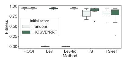
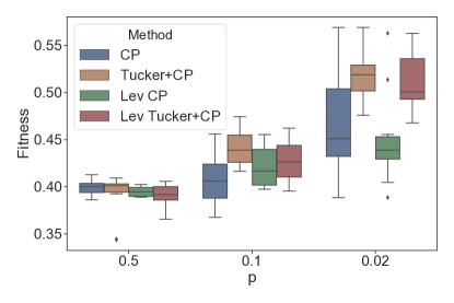
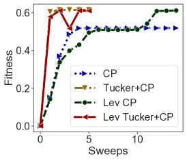
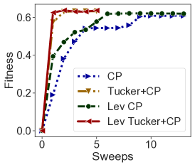
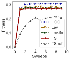
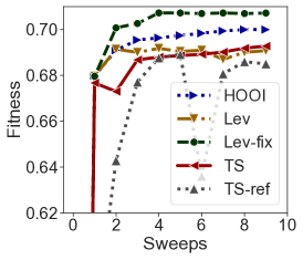
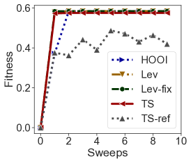
Figure 1: Detailed fitness-sweeps relation for Tucker decomposition of three dense tensors with different parameters. For Tensor 4, 𝓣𝓣\boldsymbol{\mathcal{T}} is generated based on (7.2). For all the experiments, we set R=5,α=1.6formulae-sequence𝑅5𝛼1.6R=5,\alpha=1.6, and K=16𝐾16K=16. In the plots, Lev, Lev-fix, and TS denote our new sketched Tucker-ALS scheme with leverage score random sampling, leverage score deterministic sampling, and TensorSketch, respectively. TS-ref denotes the reference sketched Tucker-ALS algorithm with TensorSketch. HOOI is initialized with HOSVD, and all other methods are initialized with RRF (Algorithm 3). Markers represent the results per sweep.
Refer to caption
(a) Tensor 1 with α=1.2,K=16formulae-sequence𝛼1.2𝐾16\alpha=1.2,K=16
Refer to caption
(b) Tensor 1 with α=1.2𝛼1.2\alpha=1.2 and HOSVD/RRF init
Refer to caption
(c) Tensor 1 with α=1.6,K=16formulae-sequence𝛼1.6𝐾16\alpha=1.6,K=16
Refer to caption
(d) Tensor 1 with α=1.6𝛼1.6\alpha=1.6 and HOSVD/RRF init
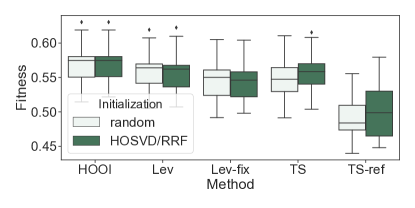
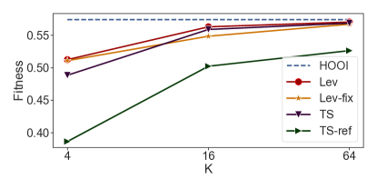
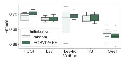
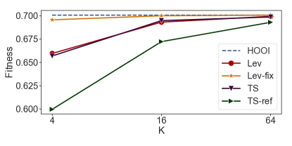
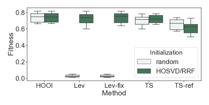
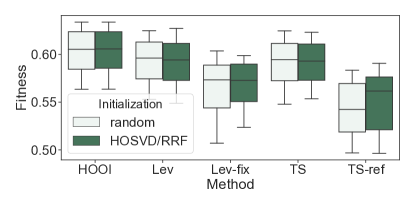
Figure 2: Experimental results for Tucker decomposition of Tensor 1. For all the experiments, we set s=200𝑠200s=200 and R=5𝑅5R=5. HOSVD/RRF means HOOI is initialized with HOSVD, and all other methods are initialized with RRF (Algorithm 3). (a)(c) Box plots of the final fitness for each algorithm with different input tensors. Each box is based on 10 experiments with different random seeds. Each box shows the 25th-75th quartiles, the median is indicated by a horizontal line inside the box, and outliers are displayed as dots. (b)(d) Relation between the final fitness and sketch size parameter K𝐾K for each algorithm with different input tensors. Each data point is the mean of 10 experimental results with different random seeds.
Refer to caption
(a) Tensor 2 with α=1.6,K=16,s=200formulae-sequence𝛼1.6formulae-sequence𝐾16𝑠200\alpha=1.6,K=16,s=200
Refer to caption
(b) Tensor 2 with α=1.6,s=200formulae-sequence𝛼1.6𝑠200\alpha=1.6,s=200 and HOSVD/RRF init
Refer to caption
(c) Tensor 4 with α=1.6,K=16formulae-sequence𝛼1.6𝐾16\alpha=1.6,K=16, s=1000𝑠1000s=1000
Refer to caption
(d) Tensor 4 with α=1.6,s=1000formulae-sequence𝛼1.6𝑠1000\alpha=1.6,s=1000 and HOSVD/RRF init
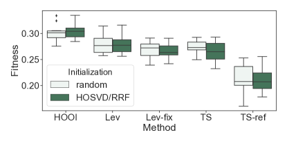
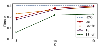
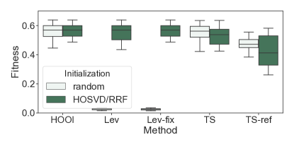
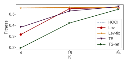
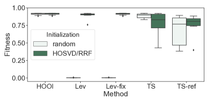
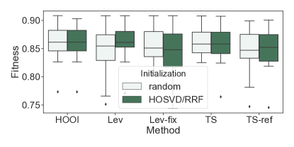
Figure 3: Experimental results for Tucker decomposition of dense tensors. For Tensor 4, 𝓣𝓣\boldsymbol{\mathcal{T}} is generated based on (7.2). For all the experiments, we set R=5𝑅5R=5. (a)(c) Box plots of the final fitness for each algorithm with different input tensors. Each box is based on 10 experiments with different random seeds. (b)(d) Relation between the final fitness and sketch size parameter K𝐾K for each algorithm with different input tensors.

7.1.1 Experimental Results for Dense Tensors

We show the detailed fitness-sweeps relation for different dense tensors in Fig. 1. The reference randomized algorithm suffers from unstable convergence as well as low fitness, while our new randomized ALS scheme, with either leverage score sampling or TensorSketch, converges faster than the reference randomized algorithm and reaches higher accuracy.

We show the final fitness for each method on different dense tensors in Fig. 2 and Fig. 3. For Tensor 1, we test on two different values of the true rank versus decomposition rank ratio, α𝛼\alpha. We do not report the results for α=1𝛼1\alpha=1, which corresponds to the exact Tucker decomposition, since all the randomized algorithms can find the exact decomposition easily. We also test on Tensor 2 and Tensor 4. As can be seen in the figure, our new randomized ALS scheme, with either leverage score sampling or TensorSketch, outperforms the reference randomized algorithm for all the tensors. The relative fitness improvement ranges from 4.5%percent4.54.5\% (Fig. 3a,3b) to 22.0%percent22.022.0\% (Fig. 2c,2d) when K=16𝐾16K=16.

Fig. 2b,2d,3b,3d show the relation between the final fitness and K𝐾K. As is expected, increasing K𝐾K can increase the accuracy of the randomized linear least squares solve, thus improving the final fitness. With our new randomized scheme, the relative final fitness difference between HOOI and the randomized algorithms is less than 8.5%percent8.58.5\% when K=16𝐾16K=16, indicating the efficacy of our new scheme.

Fig. 2a,2c,3a,3c include a comparison between random initialization and the initialization scheme based on RRF detailed in Algorithm 3. For Tensor 1, both initialization schemes have similar performance. For the deterministic leverage score sampling on Tensor 2 (Fig. 3a), using RRF-based initialization substantially decreases variability of attained accuracy. For leverage score sampling on Tensor 4 (Fig. 3c), we observe that the random initialization is not effective, resulting in approximately zero final fitness. This is because the random initializations are far from the accurate solutions, and some elements with large amplitudes are not sampled in all the ALS sweeps, consistent with our discussion in Section 5. With the RRF-based initialization, the output fitness of the algorithms based on leverage score sampling is close to HOOI. Therefore, our proposed initialization scheme is important for improving the robustness of leverage score sampling.

Although leverage score sampling has a better sketch size upper bound, based on analysis in Section 4, the random leverage score sampling scheme performs similar to TensorSketch for the tested dense tensors. For leverage score sampling, Fig. 3b,3d shows that when the sketch size is small (K=4𝐾4K=4), the deterministic leverage score sampling scheme outperforms the random sampling scheme for Tensor 2 and Tensor 4. This means that when the tensor has a strong low-rank signal, the deterministic sampling scheme can be better, consistent with the results in [44].

7.1.2 Experimental Results for Sparse Tensors
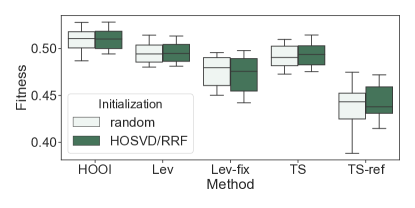
Refer to caption
(a) Tensor 3 with p=0.5𝑝0.5p=0.5
Refer to caption
(b) Tensor 4 with p=0.5𝑝0.5p=0.5
Refer to caption
(c) Tensor 3 with p=0.1𝑝0.1p=0.1
Refer to caption
(d) Tensor 4 with p=0.1𝑝0.1p=0.1
Refer to caption
(e) Tensor 3 with p=0.02𝑝0.02p=0.02
Refer to caption
(f) Tensor 4 with p=0.02𝑝0.02p=0.02
Figure 4: Experimental results for Tucker decomposition of sparse tensors. For all the experiments, we set s=2000,R=10,α=1.2formulae-sequence𝑠2000formulae-sequence𝑅10𝛼1.2s=2000,R=10,\alpha=1.2 and K=16𝐾16K=16. (a)(c)(e) Box plots of the final fitness for each algorithm on Tensor 3 with different sparsity parameter p𝑝p. (b)(d)(f) Box plots of the final fitness for each algorithm on Tensor 4 with different sparsity parameter p𝑝p. Each box is based on 10 experiments with different random seeds.

We show our experimental results for sparse tensors in Fig. 4. For both Tensor 3 and Tensor 4, we test on tensors with different sparsity via varying the parameter p𝑝p. When p=0.1𝑝0.1p=0.1 (Fig. 4c, 4d), the expected sparsity of the tensor is greater than 0.9. When p=0.02𝑝0.02p=0.02 (Fig. 4e, 4f), the expected sparsity of the tensor is greater than 0.99980.99980.9998.

The results for Tensor 3 are shown in Fig. 4a,4c,4e. Our new randomized ALS scheme, with either leverage score sampling or TensorSketch, outperforms the reference randomized algorithm with p=0.1𝑝0.1p=0.1 and p=0.5𝑝0.5p=0.5. The relative fitness improvement ranges from 3.6%percent3.63.6\% (Fig. 4c) to 12.7%percent12.712.7\% (Fig. 4a). The performance of our new scheme is comparable to the reference with p=0.02𝑝0.02p=0.02. The reason for the reduced improvements is that these tensors have high decomposition fitness (0.80.9similar-to0.80.90.8\sim 0.9) and each non-zero element has the same distribution, so sophisticated sampling is not needed to achieve high accuracy. Similar to the case of dense tensors shown in Fig. 2a,2c, we observe similar behavior for Tensor 3 with random initialization and RRF-based initialization.

The results for Tensor 4 are shown in Fig. 4b,4d,4f. Our new randomized ALS scheme outperforms the reference randomized algorithm for all the cases. Similar to the case of dense tensors (Fig. 3c), for leverage score sampling, the random initialization results in approximately zero final fitness, and the RRF-based initialization can greatly improve the output fitness. Therefore, the RRF-based initialization scheme is important for improving the robustness of leverage score sampling.

On the contrary, TensorSketch based algorithms are not sensitive to the choice of initialization scheme. Although they perform much better compared to the leverage score sampling with random initialization, the output fitness is still a bit worse than HOOI and can have relatively larger variance (Fig. 4d,4f). This means TensorSketch is less effective than leverage score sampling with RRF initialization for this tensor.

In summary, we observe the algorithm combining leverage score sampling, the RRF-based initialization and our new ALS scheme achieves the highest accuracy and the most robust performance across test problems among randomized schemes.

7.2 Experiments for CP Decomposition
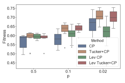
Refer to caption
(a) α=1.2𝛼1.2\alpha=1.2
Refer to caption
(b) α=1.6𝛼1.6\alpha=1.6
Figure 5: Relation between final fitness and sparsity parameter p𝑝p for CP decomposition. For all the experiments, we set s=2000,R=10formulae-sequence𝑠2000𝑅10s=2000,R=10 and K=16𝐾16K=16. In the plots, CP denotes running CP-ALS, Tucker+CP denotes running the Tucker HOOI + CP-ALS algorithm, Lev CP denotes running leverage score sampling based randomized CP-ALS, and Lev Tucker+CP denotes running the leverage score sampling based Tucker-ALS + CP-ALS algorithm. Each box is based on 10 experiments with different random seeds.
Refer to caption
(a) p=0.5𝑝0.5p=0.5
Refer to caption
(b) p=0.1𝑝0.1p=0.1
Refer to caption
(c) p=0.02𝑝0.02p=0.02
Figure 6: Detailed fitness-sweeps relation for CP decomposition of three tensors with different parameters. For all the experiments, we set s=2000,R=10,α=1.2formulae-sequence𝑠2000formulae-sequence𝑅10𝛼1.2s=2000,R=10,\alpha=1.2 and K=16𝐾16K=16. Markers represent the results per sweep. For Tucker + CP algorithms, the fitness shown for i𝑖ith sweep is the output fitness after running i𝑖i Tucker sweeps along with 25 CP-ALS sweeps on core tensors afterwards.

We show the efficacy of accelerating CP decomposition via performing Tucker compression first. We compare four different algorithms, the standard CP-ALS algorithm, the Tucker HOOI + CP-ALS algorithm, sketched CP-ALS, where the sketching matrix is applied to each linear least squares subproblem (2.6), as well as the sketched Tucker-ALS + CP-ALS algorithm shown in Algorithm 6. Random leverage score sampling is used for sketching, since it has been shown to be efficient for both Tucker (Section 7.1) and CP (reference [31]) decompositions. We use the following synthetic tensor to evaluate these four algorithms,

𝓣=i=1Rtrue𝐚i(1)𝐚i(2)𝐚i(3),𝓣superscriptsubscript𝑖1subscript𝑅truesubscriptsuperscript𝐚1𝑖subscriptsuperscript𝐚2𝑖subscriptsuperscript𝐚3𝑖\boldsymbol{\mathcal{T}}=\sum_{i=1}^{R_{\text{true}}}\mathbf{a}^{(1)}_{i}\circ\mathbf{a}^{(2)}_{i}\circ\mathbf{a}^{(3)}_{i}, (7.6)

where each element in 𝐚i(j)subscriptsuperscript𝐚𝑗𝑖\mathbf{a}^{(j)}_{i} is an i.i.d normally distributed random variable 𝒩(0,1)𝒩01\mathcal{N}(0,1) with probability p𝑝p and is zero otherwise. This guarantees that the expected sparsity of 𝓣𝓣\boldsymbol{\mathcal{T}} is lower-bounded by 1Rtruep31subscript𝑅truesuperscript𝑝31-R_{\text{true}}p^{3}. The ratio Rtrue/Rsubscript𝑅true𝑅R_{\text{true}}/R, where R𝑅R is the decomposition rank, is denoted as α𝛼\alpha.

For (sketched) Tucker + CP algorithms, we run 5 (sketched) Tucker-ALS sweeps first, and then run the CP-ALS algorithm on the core tensor for 25 sweeps. RRF-based initialization is used for Tucker-ALS, and HOSVD on the core tensor is used to initialize the factor matrices of the small CP decomposition problem. For (sketched) CP-ALS algorithms, we also use the RRF-based initialization and run 30 sweeps afterwards, which is sufficient for CP-ALS to converge based on our experiments. This initialization makes sure that leverage score sampling is effective for sparse tensors. We set the sketch size as KR2𝐾superscript𝑅2KR^{2} for both algorithms. The constant factor K𝐾K reveals the accuracy of each subproblem. For the RRF-based initialization, we set the sketch size (k𝑘k in Algorithm 3) as KR𝐾𝑅\sqrt{K}R.

We show the relation between final fitness and the tensor sparsity parameter, p𝑝p, in Fig. 5. As can be seen, for all the tested tensors, the Tucker + CP algorithms perform similarly, and usually better than directly performing CP decomposition. When the input tensor is sparse (p=0.1𝑝0.1p=0.1 and 0.020.020.02), the advantage of the Tucker + CP algorithms is greater. The sketched Tucker-ALS + CP-ALS scheme has a comparable performance compared to Tucker HOOI + CP-ALS, while requiring less computation.

We show the detailed fitness-sweeps relation in Fig. 6. We observe that for (sketched) CP-ALS, more than 10 sweeps are necessary for the algorithms to converge. On the contrary, less than 5 Tucker-ALS sweeps are needed for the sketched Tucker + CP scheme, making it more efficient.

In summary, we observe CP decomposition can be more efficiently and accurately calculated based on the sketched Tucker + CP method.

8 Conclusions

In this work, we propose a fast and accurate sketching based ALS algorithm for Tucker decomposition, which consists of a sequence of sketched rank-constrained linear least squares subproblems. Theoretical sketch size upper bounds are provided to achieve 𝒪(ϵ)𝒪italic-ϵ\mathcal{O}\left(\epsilon\right)-relative residual norm error for each subproblem with two sketching techniques, TensorSketch and leverage score sampling. For both techniques, our bounds are at most 𝒪(1/ϵ)𝒪1italic-ϵ\mathcal{O}\left(1/\epsilon\right) times the sketch size upper bounds for the unconstrained linear least squares problem. We also propose an initialization scheme based on randomized range finder to improve the accuracy of leverage score sampling based randomized Tucker decomposition of tensors with high coherence. Experimental results show that this new ALS algorithm is more accurate than the existing sketching based randomized algorithm for Tucker decomposition. This Tucker decomposition algorithm also yields an efficient CP decomposition method, where randomized Tucker compression is performed first, and CP decomposition is applied to the Tucker core tensor afterwards. Experimental results show this algorithm not only converges faster, but also yields more accurate CP decompositions.

We leave high-performance implementation of our sketched ALS algorithm as well as testing its performance on large-scale real sparse datasets for future work. Additionally, although our theoretical analysis shows a much tighter sketch size upper bound for leverage score sampling compared to TensorSketch, their experimental performance under the same sketch size for multiple tensors are similar. Therefore, it will be of interest to investigate potential improvements to sketch size bounds for TensorSketch.

References

  • [1] K. S. Aggour, A. Gittens, and B. Yener. Adaptive sketching for fast and convergent canonical polyadic decomposition. In International Conference on Machine Learning. PMLR, 2020.
  • [2] S. Ahmadi-Asl, S. Abukhovich, M. G. Asante-Mensah, A. Cichocki, A. H. Phan, T. Tanaka, and I. Oseledets. Randomized algorithms for computation of Tucker decomposition and higher order SVD (HOSVD). IEEE Access, 9:28684–28706, 2021.
  • [3] A. Anandkumar, R. Ge, D. Hsu, S. M. Kakade, and M. Telgarsky. Tensor decompositions for learning latent variable models. Journal of Machine Learning Research, 15:2773–2832, 2014.
  • [4] C. A. Andersson and R. Bro. Improving the speed of multi-way algorithms: Part I. Tucker3. Chemometrics and intelligent laboratory systems, 42(1-2):93–103, 1998.
  • [5] H. Avron, K. L. Clarkson, and D. P. Woodruff. Sharper bounds for regularized data fitting. arXiv preprint arXiv:1611.03225, 2016.
  • [6] C. Battaglino, G. Ballard, and T. G. Kolda. A practical randomized CP tensor decomposition. SIAM Journal on Matrix Analysis and Applications, 39(2):876–901, 2018.
  • [7] C. Boutsidis and D. Woodruff. Communication-optimal distributed principal component analysis in the column-partition model. arXiv preprint arXiv:1504.06729, 2015.
  • [8] R. Bro and C. A. Andersson. Improving the speed of multiway algorithms: Part II: Compression. Chemometrics and intelligent laboratory systems, 42(1-2):105–113, 1998.
  • [9] E. J. Candès and B. Recht. Exact matrix completion via convex optimization. Foundations of Computational mathematics, 9(6):717, 2009.
  • [10] J. D. Carroll, S. Pruzansky, and J. B. Kruskal. CANDELINC: A general approach to multidimensional analysis of many-way arrays with linear constraints on parameters. Psychometrika, 45(1):3–24, 1980.
  • [11] M. Che and Y. Wei. Randomized algorithms for the approximations of Tucker and the tensor train decompositions. Advances in Computational Mathematics, 45(1):395–428, 2019.
  • [12] M. Che, Y. Wei, and H. Yan. Randomized algorithms for the low multilinear rank approximations of tensors. Journal of Computational and Applied Mathematics, page 113380, 2021.
  • [13] D. Cheng, R. Peng, Y. Liu, and I. Perros. SPALS: Fast alternating least squares via implicit leverage scores sampling. Advances in neural information processing systems, 29:721–729, 2016.
  • [14] L. De Lathauwer, B. De Moor, and J. Vandewalle. A multilinear singular value decomposition. SIAM journal on Matrix Analysis and Applications, 21(4):1253–1278, 2000.
  • [15] L. De Lathauwer, B. De Moor, and J. Vandewalle. On the best rank-1 and rank-(r1, r2,…, rn) approximation of higher-order tensors. SIAM journal on Matrix Analysis and Applications, 21(4):1324–1342, 2000.
  • [16] H. Diao, Z. Song, W. Sun, and D. Woodruff. Sketching for Kronecker product regression and p-splines. In International Conference on Artificial Intelligence and Statistics, pages 1299–1308. PMLR, 2018.
  • [17] P. Drineas, M. Magdon-Ismail, M. W. Mahoney, and D. P. Woodruff. Fast approximation of matrix coherence and statistical leverage. The Journal of Machine Learning Research, 13(1):3475–3506, 2012.
  • [18] P. Drineas, M. W. Mahoney, S. Muthukrishnan, and T. Sarlós. Faster least squares approximation. Numerische mathematik, 117(2):219–249, 2011.
  • [19] N. B. Erichson, K. Manohar, S. L. Brunton, and J. N. Kutz. Randomized CP tensor decomposition. Machine Learning: Science and Technology, 1(2):025012, 2020.
  • [20] M. Gu and S. C. Eisenstat. Efficient algorithms for computing a strong rank-revealing QR factorization. SIAM Journal on Scientific Computing, 17(4):848–869, 1996.
  • [21] N. Halko, P.-G. Martinsson, and J. A. Tropp. Finding structure with randomness: Probabilistic algorithms for constructing approximate matrix decompositions. SIAM review, 53(2):217–288, 2011.
  • [22] R. A. Harshman. Foundations of the PARAFAC procedure: models and conditions for an explanatory multimodal factor analysis. 1970.
  • [23] F. L. Hitchcock. The expression of a tensor or a polyadic as a sum of products. Studies in Applied Mathematics, 6(1-4):164–189, 1927.
  • [24] E. G. Hohenstein, R. M. Parrish, and T. J. Martínez. Tensor hypercontraction density fitting. I. Quartic scaling second-and third-order Møller-Plesset perturbation theory. The Journal of chemical physics, 137(4):044103, 2012.
  • [25] F. Hummel, T. Tsatsoulis, and A. Grüneis. Low rank factorization of the Coulomb integrals for periodic coupled cluster theory. The Journal of chemical physics, 146(12):124105, 2017.
  • [26] R. Jin, T. G. Kolda, and R. Ward. Faster Johnson-Lindenstrauss transforms via Kronecker products. arXiv preprint arXiv:1909.04801, 2019.
  • [27] I. T. Jolliffe. Discarding variables in a principal component analysis. I: Artificial data. Journal of the Royal Statistical Society: Series C (Applied Statistics), 21(2):160–173, 1972.
  • [28] O. Kaya and B. Uçar. High performance parallel algorithms for the Tucker decomposition of sparse tensors. In 2016 45th International Conference on Parallel Processing (ICPP), pages 103–112. IEEE, 2016.
  • [29] O. Kaya and B. Uçar. Parallel CANDECOMP/PARAFAC decomposition of sparse tensors using dimension trees. SIAM Journal on Scientific Computing, 40(1):C99–C130, 2018.
  • [30] T. G. Kolda and B. W. Bader. Tensor decompositions and applications. SIAM review, 51(3):455–500, 2009.
  • [31] B. W. Larsen and T. G. Kolda. Practical leverage-based sampling for low-rank tensor decomposition. arXiv preprint arXiv:2006.16438, 2020.
  • [32] H. Li, Z. Li, K. Li, J. S. Rellermeyer, L. Chen, and K. Li. SGD_Tucker: A novel stochastic optimization strategy for parallel sparse Tucker decomposition. arXiv preprint arXiv:2012.03550, 2020.
  • [33] J. Li, J. Choi, I. Perros, J. Sun, and R. Vuduc. Model-driven sparse CP decomposition for higher-order tensors. In 2017 IEEE international parallel and distributed processing symposium (IPDPS), pages 1048–1057. IEEE, 2017.
  • [34] L. Ma and E. Solomonik. Accelerating alternating least squares for tensor decomposition by pairwise perturbation. arXiv preprint arXiv:1811.10573, 2018.
  • [35] L. Ma and E. Solomonik. Efficient parallel CP decomposition with pairwise perturbation and multi-sweep dimension tree. arXiv preprint arXiv:2010.12056, 2020.
  • [36] M. W. Mahoney. Randomized algorithms for matrices and data. arXiv preprint arXiv:1104.5557, 2011.
  • [37] O. A. Malik and S. Becker. Low-rank Tucker decomposition of large tensors using Tensorsketch. Advances in neural information processing systems, 31:10096–10106, 2018.
  • [38] R. Minster, A. K. Saibaba, and M. E. Kilmer. Randomized algorithms for low-rank tensor decompositions in the Tucker format. SIAM Journal on Mathematics of Data Science, 2(1):189–215, 2020.
  • [39] L. Mirsky. Symmetric gauge functions and unitarily invariant norms. The quarterly journal of mathematics, 11(1):50–59, 1960.
  • [40] B. C. Mitchell and D. S. Burdick. Slowly converging PARAFAC sequences: swamps and two-factor degeneracies. Journal of Chemometrics, 8(2):155–168, 1994.
  • [41] I. Nisa, J. Li, A. Sukumaran-Rajam, R. Vuduc, and P. Sadayappan. Load-balanced sparse MTTKRP on GPUs. In 2019 IEEE International Parallel and Distributed Processing Symposium (IPDPS), pages 123–133. IEEE, 2019.
  • [42] S. Oh, N. Park, S. Lee, and U. Kang. Scalable Tucker factorization for sparse tensors-algorithms and discoveries. In 2018 IEEE 34th International Conference on Data Engineering (ICDE), pages 1120–1131. IEEE, 2018.
  • [43] R. Pagh. Compressed matrix multiplication. ACM Transactions on Computation Theory (TOCT), 5(3):1–17, 2013.
  • [44] D. Papailiopoulos, A. Kyrillidis, and C. Boutsidis. Provable deterministic leverage score sampling. In Proceedings of the 20th ACM SIGKDD international conference on Knowledge discovery and data mining, pages 997–1006, 2014.
  • [45] W. Pazner and P.-O. Persson. Approximate tensor-product preconditioners for very high order discontinuous Galerkin methods. Journal of Computational Physics, 354:344–369, 2018.
  • [46] M. Pilanci and M. J. Wainwright. Iterative Hessian sketch: fast and accurate solution approximation for constrained least-squares. The Journal of Machine Learning Research, 17(1):1842–1879, 2016.
  • [47] N. D. Sidiropoulos, L. De Lathauwer, X. Fu, K. Huang, E. E. Papalexakis, and C. Faloutsos. Tensor decomposition for signal processing and machine learning. IEEE Transactions on Signal Processing, 65(13):3551–3582.
  • [48] S. Smith and G. Karypis. A medium-grained algorithm for sparse tensor factorization. In 2016 IEEE International Parallel and Distributed Processing Symposium (IPDPS), pages 902–911. IEEE, 2016.
  • [49] S. Smith, N. Ravindran, N. D. Sidiropoulos, and G. Karypis. SPLATT: Efficient and parallel sparse tensor-matrix multiplication. In 2015 IEEE International Parallel and Distributed Processing Symposium, pages 61–70. IEEE, 2015.
  • [50] Z. Song, D. P. Woodruff, and P. Zhong. Relative error tensor low rank approximation. In Proceedings of the Thirtieth Annual ACM-SIAM Symposium on Discrete Algorithms, pages 2772–2789. SIAM, 2019.
  • [51] Y. Sun, Y. Guo, C. Luo, J. Tropp, and M. Udell. Low-rank Tucker approximation of a tensor from streaming data. SIAM Journal on Mathematics of Data Science, 2(4):1123–1150, 2020.
  • [52] Y. Sun, Y. Guo, J. A. Tropp, and M. Udell. Tensor random projection for low memory dimension reduction. In NeurIPS Workshop on Relational Representation Learning, 2018.
  • [53] L. R. Tucker. Some mathematical notes on three-mode factor analysis. Psychometrika, 31(3):279–311, 1966.
  • [54] S. Wang. A practical guide to randomized matrix computations with MATLAB implementations. arXiv preprint arXiv:1505.07570, 2015.
  • [55] D. P. Woodruff. Sketching as a tool for numerical linear algebra. arXiv preprint arXiv:1411.4357, 2014.
  • [56] G. Zhou, A. Cichocki, and S. Xie. Decomposition of big tensors with low multilinear rank. arXiv preprint arXiv:1412.1885, 2014.

Appendix A Detailed Proofs for Section 4

In this section, we provide detailed proofs for the sketch size upper bounds of both sketched unconstrained and rank-constrained linear least squares problems. In Section A.1, we define the (γ,δ,ϵ)𝛾𝛿italic-ϵ(\gamma,\delta,\epsilon)-accurate sketching matrix, and show the error bound for sketched unconstrained linear least squares, under the assumption that the sketching matrix is a (1/2,δ,ϵ)12𝛿italic-ϵ(1/2,\delta,\epsilon)-accurate sketching matrix. In Section A.2, we show the error bound for sketched rank-constrained linear least squares. In Section A.3 and Section A.4, we finish the proofs by giving the sketch size bounds that are sufficient for the TensorSketch matrix and leverage score sampling matrix to be the (1/2,δ,ϵ)12𝛿italic-ϵ(1/2,\delta,\epsilon)-accurate sketching matrix, respectively.

A.1 Error Bound for Sketched Unconstrained Linear Least Squares

We define the (γ,δ,ϵ)𝛾𝛿italic-ϵ(\gamma,\delta,\epsilon)-accurate sketching matrix in Definition 6. In Lemma A.1, we show the relative error bound for the unconstrained linear least squares problem with a (1/2,δ,ϵ)12𝛿italic-ϵ(1/2,\delta,\epsilon)-accurate sketching matrix. By 𝐐Psubscript𝐐𝑃\mathbf{Q}_{P} we denote a matrix whose columns form an orthonormal basis for the column space of 𝐏𝐏\mathbf{P}.

Definition 6 ((γ,δ,ϵ)𝛾𝛿italic-ϵ(\gamma,\delta,\epsilon)-accurate Sketching Matrix).

A random matrix 𝐒m×s𝐒superscript𝑚𝑠\mathbf{S}\in\mathbb{R}^{m\times s} is a (γ,δ,ϵ)𝛾𝛿italic-ϵ(\gamma,\delta,\epsilon)-accurate sketching matrix for 𝐏s×R𝐏superscript𝑠𝑅\mathbf{P}\in\mathbb{R}^{s\times R} if the following two conditions hold simultaneously.

  1. 1.

    With probability at least 1δ/21𝛿21-\delta/2, each singular value σ𝜎\sigma of 𝐒𝐐Psubscript𝐒𝐐𝑃\mathbf{SQ}_{P} satisfies

    1γσ21+γ.1𝛾superscript𝜎21𝛾1-\gamma\leq\sigma^{2}\leq 1+\gamma. (A.1)
  2. 2.

    With probability at least 1δ/21𝛿21-\delta/2, for any fixed matrix 𝐁𝐁\mathbf{B}, we have

    𝐐PT𝐒T𝐒𝐁𝐐PT𝐁F2ϵ2𝐁F2.superscriptsubscriptnormsuperscriptsubscript𝐐𝑃𝑇superscript𝐒𝑇𝐒𝐁superscriptsubscript𝐐𝑃𝑇𝐁𝐹2superscriptitalic-ϵ2superscriptsubscriptnorm𝐁𝐹2\|\mathbf{Q}_{P}^{T}\mathbf{S}^{T}\mathbf{SB}-\mathbf{Q}_{P}^{T}\mathbf{B}\|_{F}^{2}\leq\epsilon^{2}\cdot\|\mathbf{B}\|_{F}^{2}. (A.2)
Lemma A.1 (Linear Least Squares with (1/2,δ,ϵ)12𝛿italic-ϵ(1/2,\delta,\epsilon)-accurate Sketching Matrix [55, 31, 18]).

Given a full-rank matrix 𝐏s×R𝐏superscript𝑠𝑅\mathbf{P}\in\mathbb{R}^{s\times R} with sR𝑠𝑅s\geq R, and 𝐁s×n𝐁superscript𝑠𝑛\mathbf{B}\in\mathbb{R}^{s\times n}. Let 𝐒m×s𝐒superscript𝑚𝑠\mathbf{S}\in\mathbb{R}^{m\times s} be a (1/2,δ,ϵ)12𝛿italic-ϵ(1/2,\delta,\epsilon)-accurate sketching matrix. Let 𝐁=𝐏𝐗opt𝐁superscript𝐁perpendicular-tosubscript𝐏𝐗opt𝐁\mathbf{B}^{\perp}=\mathbf{P}\mathbf{X}_{\text{opt}}-\mathbf{B}, with 𝐗opt=argmin𝐗𝐏𝐗𝐁Fsubscript𝐗optsubscript𝐗subscriptnorm𝐏𝐗𝐁𝐹\mathbf{X}_{\text{opt}}=\arg\min_{\mathbf{X}}\left\|\mathbf{PX}-\mathbf{B}\right\|_{F}, and 𝐗~opt=argmin𝐗𝐒𝐏𝐗𝐒𝐁Fsubscript~𝐗optsubscript𝐗subscriptnorm𝐒𝐏𝐗𝐒𝐁𝐹\mathbf{\widetilde{X}}_{\text{opt}}=\arg\min_{\mathbf{X}}{\|\mathbf{SPX}-\mathbf{SB}\|}_{F}. Then the following approximation holds with probability at least 1δ1𝛿1-\delta,

𝐏𝐗~opt𝐏𝐗optF2𝒪(ϵ2)𝐁F2.superscriptsubscriptnorm𝐏subscript~𝐗optsubscript𝐏𝐗opt𝐹2𝒪superscriptitalic-ϵ2superscriptsubscriptnormsuperscript𝐁perpendicular-to𝐹2\left\|\mathbf{P}\mathbf{\widetilde{X}}_{\text{opt}}-\mathbf{P}\mathbf{X}_{\text{opt}}\right\|_{F}^{2}\leq\mathcal{O}\left(\epsilon^{2}\right)\left\|\mathbf{B}^{\perp}\right\|_{F}^{2}. (A.3)
Proof.

Define the reduced QR decomposition, 𝐏=𝐐P𝐑P𝐏subscript𝐐𝑃subscript𝐑𝑃\mathbf{P}=\mathbf{Q}_{P}\mathbf{R}_{P}. The unconstrained sketched problem can be rewritten as

min𝐗𝐒𝐏𝐗𝐒𝐁Fsubscript𝐗subscriptnorm𝐒𝐏𝐗𝐒𝐁𝐹\displaystyle\min_{\mathbf{X}}\left\|\mathbf{SPX}-\mathbf{SB}\right\|_{F} =min𝐗𝐒𝐏𝐗𝐒(𝐏𝐗opt+𝐁)Fabsentsubscript𝐗subscriptnorm𝐒𝐏𝐗𝐒subscript𝐏𝐗optsuperscript𝐁perpendicular-to𝐹\displaystyle=\min_{\mathbf{X}}\left\|\mathbf{SPX}-\mathbf{S}(\mathbf{P}\mathbf{X}_{\text{opt}}+\mathbf{B}^{\perp})\right\|_{F}
=min𝐗𝐒𝐐P𝐑P(𝐗𝐗opt)𝐒𝐁F,absentsubscript𝐗subscriptnormsubscript𝐒𝐐𝑃subscript𝐑𝑃𝐗subscript𝐗optsuperscript𝐒𝐁perpendicular-to𝐹\displaystyle=\min_{\mathbf{X}}\left\|\mathbf{S}\mathbf{Q}_{P}\mathbf{R}_{P}(\mathbf{X}-\mathbf{X}_{\text{opt}})-\mathbf{S}\mathbf{B}^{\perp}\right\|_{F},

thus the optimality condition is

(𝐒𝐐P)T𝐒𝐐P𝐑P(𝐗~opt𝐗opt)=(𝐒𝐐P)T𝐒𝐁.superscriptsubscript𝐒𝐐𝑃𝑇subscript𝐒𝐐𝑃subscript𝐑𝑃subscript~𝐗optsubscript𝐗optsuperscriptsubscript𝐒𝐐𝑃𝑇superscript𝐒𝐁perpendicular-to(\mathbf{S}\mathbf{Q}_{P})^{T}\mathbf{S}\mathbf{Q}_{P}\mathbf{R}_{P}(\mathbf{\widetilde{X}}_{\text{opt}}-\mathbf{X}_{\text{opt}})=(\mathbf{S}\mathbf{Q}_{P})^{T}\mathbf{S}\mathbf{B}^{\perp}. (A.4)

Based on (A.1),(A.2), with probability at least 1δ1𝛿1-\delta, both of the following hold,

σmin2(𝐒𝐐P)1γ=1/2,superscriptsubscript𝜎2subscript𝐒𝐐𝑃1𝛾12\displaystyle\sigma_{\min}^{2}(\mathbf{S}\mathbf{Q}_{P})\geq 1-\gamma=1/2, (A.5)
𝐐PT𝐒T𝐒𝐁F2=𝐐PT𝐒T𝐒𝐁𝐐PT𝐁F2ϵ2𝐁F2,superscriptsubscriptnormsuperscriptsubscript𝐐𝑃𝑇superscript𝐒𝑇superscript𝐒𝐁perpendicular-to𝐹2superscriptsubscriptnormsuperscriptsubscript𝐐𝑃𝑇superscript𝐒𝑇superscript𝐒𝐁perpendicular-tosuperscriptsubscript𝐐𝑃𝑇superscript𝐁perpendicular-to𝐹2superscriptitalic-ϵ2superscriptsubscriptnormsuperscript𝐁perpendicular-to𝐹2\displaystyle\left\|\mathbf{Q}_{P}^{T}\mathbf{S}^{T}\mathbf{S}\mathbf{B}^{\perp}\right\|_{F}^{2}=\left\|\mathbf{Q}_{P}^{T}\mathbf{S}^{T}\mathbf{S}\mathbf{B}^{\perp}-\mathbf{Q}_{P}^{T}\mathbf{B}^{\perp}\right\|_{F}^{2}\leq\epsilon^{2}\cdot\left\|\mathbf{B}^{\perp}\right\|_{F}^{2}, (A.6)

where σmin(𝐒𝐐P)subscript𝜎subscript𝐒𝐐𝑃\sigma_{\min}(\mathbf{S}\mathbf{Q}_{P}) is the singular value of 𝐒𝐐Psubscript𝐒𝐐𝑃\mathbf{S}\mathbf{Q}_{P} with the smallest magnitude. Combining (A.4), (A.5), and (A.6), we obtain

𝐏𝐗~opt𝐏𝐗optF2superscriptsubscriptnorm𝐏subscript~𝐗optsubscript𝐏𝐗opt𝐹2\displaystyle\left\|\mathbf{P}\mathbf{\widetilde{X}}_{\text{opt}}-\mathbf{P}\mathbf{X}_{\text{opt}}\right\|_{F}^{2} =𝐑P𝐗~opt𝐑P𝐗optF2absentsuperscriptsubscriptnormsubscript𝐑𝑃subscript~𝐗optsubscript𝐑𝑃subscript𝐗opt𝐹2\displaystyle=\left\|\mathbf{R}_{P}\mathbf{\widetilde{X}}_{\text{opt}}-\mathbf{R}_{P}\mathbf{X}_{\text{opt}}\right\|_{F}^{2}
(A.5)4(𝐒𝐐P)T𝐒𝐐P𝐑P(𝐗~opt𝐗opt)F2italic-(A.5italic-)4superscriptsubscriptnormsuperscriptsubscript𝐒𝐐𝑃𝑇subscript𝐒𝐐𝑃subscript𝐑𝑃subscript~𝐗optsubscript𝐗opt𝐹2\displaystyle\overset{\eqref{eq:structure1_theorema1}}{\leq}4\left\|(\mathbf{S}\mathbf{Q}_{P})^{T}\mathbf{S}\mathbf{Q}_{P}\mathbf{R}_{P}(\mathbf{\widetilde{X}}_{\text{opt}}-\mathbf{X}_{\text{opt}})\right\|_{F}^{2}
=(A.4)4𝐐PT𝐒T𝐒𝐁F2italic-(A.4italic-)4superscriptsubscriptnormsuperscriptsubscript𝐐𝑃𝑇superscript𝐒𝑇superscript𝐒𝐁perpendicular-to𝐹2\displaystyle\overset{\eqref{eq:opt_condition}}{=}4\left\|\mathbf{Q}_{P}^{T}\mathbf{S}^{T}\mathbf{S}\mathbf{B}^{\perp}\right\|_{F}^{2}
(A.6)4ϵ2𝐁F2=𝒪(ϵ2)𝐁F2.italic-(A.6italic-)4superscriptitalic-ϵ2superscriptsubscriptnormsuperscript𝐁perpendicular-to𝐹2𝒪superscriptitalic-ϵ2superscriptsubscriptnormsuperscript𝐁perpendicular-to𝐹2\displaystyle\overset{\eqref{eq:structure2_theorema1}}{\leq}4\epsilon^{2}\cdot\left\|\mathbf{B}^{\perp}\right\|_{F}^{2}=\mathcal{O}\left(\epsilon^{2}\right)\left\|\mathbf{B}^{\perp}\right\|_{F}^{2}.

A.2 Error Bound for Sketched Rank-constrained Linear Least Squares

We show in Theorem A.3 that with at least 1δ1𝛿1-\delta probability, the relative residual norm error for the rank-constrained linear least squares with a (1/2,δ,ϵ)12𝛿italic-ϵ(1/2,\delta,\epsilon)-accurate sketching matrix is bounded by 𝒪(ϵ)𝒪italic-ϵ\mathcal{O}\left(\epsilon\right). We first state Mirsky’s Inequality below, which bounds the perturbation of singular values when the input matrix is perturbed. We direct readers to the reference for its proof. This bound will be used in Theorem A.3.

Lemma A.2 (Mirsky’s Inequality for Perturbation of Singular Values [39]).

Let 𝐀𝐀\mathbf{A} and 𝐅𝐅\mathbf{F} be arbitrary matrices (of the same size) where σ1σnsubscript𝜎1subscript𝜎𝑛\sigma_{1}\geq\cdots\geq\sigma_{n} are the singular values of 𝐀𝐀\mathbf{A} and σ1σnsuperscriptsubscript𝜎1superscriptsubscript𝜎𝑛\sigma_{1}^{\prime}\geq\cdots\geq\sigma_{n}^{\prime} are the singular values of 𝐀+𝐅𝐀𝐅\mathbf{A}+\mathbf{F}. Then

i=1n(σiσi)2𝐅F2.superscriptsubscript𝑖1𝑛superscriptsubscript𝜎𝑖superscriptsubscript𝜎𝑖2superscriptsubscriptnorm𝐅𝐹2\sum_{i=1}^{n}(\sigma_{i}-\sigma_{i}^{\prime})^{2}\leq\|\mathbf{F}\|_{F}^{2}. (A.7)
Theorem A.3 (Rank-constrained Linear Least Squares with (1/2,δ,ϵ)12𝛿italic-ϵ(1/2,\delta,\epsilon)-accurate Sketching Matrix).

Given 𝐏s×R𝐏superscript𝑠𝑅\mathbf{P}\in\mathbb{R}^{s\times R} with orthonormal columns (such that 𝐏=𝐐P𝐏subscript𝐐𝑃\mathbf{P}=\mathbf{Q}_{P}), and 𝐁s×n𝐁superscript𝑠𝑛\mathbf{B}\in\mathbb{R}^{s\times n}. Let 𝐒m×s𝐒superscript𝑚𝑠\mathbf{S}\in\mathbb{R}^{m\times s} be a (1/2,δ,ϵ)12𝛿italic-ϵ(1/2,\delta,\epsilon)-accurate sketching matrix. Let 𝐗~rsubscript~𝐗r\mathbf{\widetilde{X}}_{\text{r}} be the best rank-r𝑟r approximation of the solution of the problem min𝐗𝐒𝐏𝐗𝐒𝐁Fsubscript𝐗subscriptnorm𝐒𝐏𝐗𝐒𝐁𝐹\min_{\mathbf{X}}{\|\mathbf{SPX}-\mathbf{SB}\|}_{F}, and let 𝐗r=argmin𝐗,rank(𝐗)=r𝐏𝐗𝐁Fsubscript𝐗rsubscript𝐗rank𝐗𝑟subscriptnorm𝐏𝐗𝐁𝐹\mathbf{X}_{\text{r}}=\arg\min_{\mathbf{X},\text{rank}(\mathbf{X})=r}\left\|\mathbf{PX}-\mathbf{B}\right\|_{F}. Then the residual norm error bound,

𝐏𝐗~r𝐁F2(1+𝒪(ϵ))𝐏𝐗r𝐁F2,superscriptsubscriptnorm𝐏subscript~𝐗r𝐁𝐹21𝒪italic-ϵsuperscriptsubscriptnormsubscript𝐏𝐗r𝐁𝐹2\left\|\mathbf{P}\mathbf{\widetilde{X}}_{\text{r}}-\mathbf{B}\right\|_{F}^{2}\leq\left(1+\mathcal{O}\left(\epsilon\right)\right)\Big{\|}\mathbf{P}\mathbf{X}_{\text{r}}-\mathbf{B}\Big{\|}_{F}^{2}, (A.8)

holds with probability at least 1δ1𝛿1-\delta.

Proof.

Let =𝐏𝐗r𝐁Fsubscriptnormsubscript𝐏𝐗r𝐁𝐹\mathcal{R}=\left\|\mathbf{P}\mathbf{X}_{\text{r}}-\mathbf{B}\right\|_{F}. In addition, let 𝐗opt=argmin𝐗𝐏𝐗𝐁Fsubscript𝐗optsubscript𝐗subscriptnorm𝐏𝐗𝐁𝐹\mathbf{X}_{\text{opt}}=\arg\min_{\mathbf{X}}\left\|\mathbf{PX}-\mathbf{B}\right\|_{F} be the optimum solution of the unconstrained linear least squares problem. Since the residual in the true solution for each component of the least-squares problem (column of 𝐁superscript𝐁perpendicular-to\mathbf{B}^{\perp}) is orthogonal to the error due to low rank approximation,

2=𝐏𝐗r𝐁F2superscript2subscriptsuperscriptnormsubscript𝐏𝐗r𝐁2𝐹\displaystyle\mathcal{R}^{2}=\left\|\mathbf{P}\mathbf{X}_{\text{r}}-\mathbf{B}\right\|^{2}_{F} =𝐏𝐗opt𝐁F2+𝐏𝐗r𝐏𝐗optF2absentsubscriptsuperscriptnormsubscript𝐏𝐗opt𝐁2𝐹subscriptsuperscriptnormsubscript𝐏𝐗rsubscript𝐏𝐗opt2𝐹\displaystyle=\left\|\mathbf{P}\mathbf{X}_{\text{opt}}-\mathbf{B}\right\|^{2}_{F}+\left\|\mathbf{P}\mathbf{X}_{\text{r}}-\mathbf{P}\mathbf{X}_{\text{opt}}\right\|^{2}_{F}
=𝐁F2+𝐗r𝐗optF2.absentsuperscriptsubscriptnormsuperscript𝐁perpendicular-to𝐹2subscriptsuperscriptnormsubscript𝐗rsubscript𝐗opt2𝐹\displaystyle=\left\|\mathbf{B}^{\perp}\right\|_{F}^{2}+\left\|\mathbf{X}_{\text{r}}-\mathbf{X}_{\text{opt}}\right\|^{2}_{F}. (A.9)

The last equality holds since 𝐏𝐏\mathbf{P} has orthonormal columns. Let 𝐗~opt=argmin𝐗𝐒𝐏𝐗𝐒𝐁Fsubscript~𝐗optsubscript𝐗subscriptnorm𝐒𝐏𝐗𝐒𝐁𝐹\mathbf{\widetilde{X}}_{\text{opt}}=\arg\min_{\mathbf{X}}\left\|\mathbf{SPX}-\mathbf{SB}\right\|_{F} be the optimum solution of the unconstrained sketched problem. We have

𝐏𝐗~r𝐁F2superscriptsubscriptnorm𝐏subscript~𝐗r𝐁𝐹2\displaystyle\left\|\mathbf{P}\mathbf{\widetilde{X}}_{\text{r}}-\mathbf{B}\right\|_{F}^{2} =𝐏𝐗~r𝐏𝐗~optF2+𝐏𝐗~opt𝐁F2+2𝐏𝐗~r𝐏𝐗~opt,𝐏𝐗~opt𝐁Fabsentsuperscriptsubscriptnorm𝐏subscript~𝐗r𝐏subscript~𝐗opt𝐹2superscriptsubscriptnorm𝐏subscript~𝐗opt𝐁𝐹22subscript𝐏subscript~𝐗r𝐏subscript~𝐗opt𝐏subscript~𝐗opt𝐁𝐹\displaystyle=\left\|\mathbf{P}\mathbf{\widetilde{X}}_{\text{r}}-\mathbf{P}\mathbf{\widetilde{X}}_{\text{opt}}\right\|_{F}^{2}+\left\|\mathbf{P}\mathbf{\widetilde{X}}_{\text{opt}}-\mathbf{B}\right\|_{F}^{2}+2\left\langle\mathbf{P}\mathbf{\widetilde{X}}_{\text{r}}-\mathbf{P}\mathbf{\widetilde{X}}_{\text{opt}},\mathbf{P}\mathbf{\widetilde{X}}_{\text{opt}}-\mathbf{B}\right\rangle_{F}
=𝐗~r𝐗~optF2+𝐗~opt𝐗optF2+𝐁F2+2𝐗~r𝐗~opt,𝐗~opt𝐗optF.absentsuperscriptsubscriptnormsubscript~𝐗rsubscript~𝐗opt𝐹2superscriptsubscriptnormsubscript~𝐗optsubscript𝐗opt𝐹2superscriptsubscriptnormsuperscript𝐁perpendicular-to𝐹22subscriptsubscript~𝐗rsubscript~𝐗optsubscript~𝐗optsubscript𝐗opt𝐹\displaystyle=\left\|\mathbf{\widetilde{X}}_{\text{r}}-\mathbf{\widetilde{X}}_{\text{opt}}\right\|_{F}^{2}+\left\|\mathbf{\widetilde{X}}_{\text{opt}}-\mathbf{X}_{\text{opt}}\right\|_{F}^{2}+\left\|\mathbf{B}^{\perp}\right\|_{F}^{2}+2\left\langle\mathbf{\widetilde{X}}_{\text{r}}-\mathbf{\widetilde{X}}_{\text{opt}},\mathbf{\widetilde{X}}_{\text{opt}}-\mathbf{X}_{\text{opt}}\right\rangle_{F}. (A.10)

Next we bound the magnitudes of the first, second and the fourth terms. According to Lemma A.1, with probability at least 1δ1𝛿1-\delta, the second term in (A.10) can be bounded as

𝐗~opt𝐗optF2=𝐏𝐗~opt𝐏𝐗optF2Cϵ2𝐁F2,superscriptsubscriptnormsubscript~𝐗optsubscript𝐗opt𝐹2superscriptsubscriptnorm𝐏subscript~𝐗optsubscript𝐏𝐗opt𝐹2𝐶superscriptitalic-ϵ2superscriptsubscriptnormsuperscript𝐁perpendicular-to𝐹2\left\|\mathbf{\widetilde{X}}_{\text{opt}}-\mathbf{X}_{\text{opt}}\right\|_{F}^{2}=\left\|\mathbf{P}\mathbf{\widetilde{X}}_{\text{opt}}-\mathbf{P}\mathbf{X}_{\text{opt}}\right\|_{F}^{2}\leq C\epsilon^{2}\left\|\mathbf{B}^{\perp}\right\|_{F}^{2}, (A.11)

for some constant C1𝐶1C\geq 1. Suppose 𝐗~optsubscript~𝐗opt\mathbf{\widetilde{X}}_{\text{opt}} has singular values σ~i=σi+δσisubscript~𝜎𝑖subscript𝜎𝑖𝛿subscript𝜎𝑖\widetilde{\sigma}_{i}=\sigma_{i}+\delta\sigma_{i} for i𝑖i in {1,,min(R,n)}1𝑅𝑛\{1,\ldots,\min(R,n)\}, where σisubscript𝜎𝑖\sigma_{i} are the singular values of 𝐗optsubscript𝐗opt\mathbf{X}_{\text{opt}}. Since 𝐗~rsubscript~𝐗r\mathbf{\widetilde{X}}_{\text{r}} is defined to be the best low rank approximation to 𝐗~optsubscript~𝐗opt\mathbf{\widetilde{X}}_{\text{opt}}, we have

𝐗~r𝐗~optF2=i=r+1min(R,n)σ~i2=i=r+1min(R,n)(σi+δσi)2=i=r+1min(R,n)(σi2+δσi2+2σiδσi).superscriptsubscriptnormsubscript~𝐗rsubscript~𝐗opt𝐹2superscriptsubscript𝑖𝑟1𝑅𝑛superscriptsubscript~𝜎𝑖2superscriptsubscript𝑖𝑟1𝑅𝑛superscriptsubscript𝜎𝑖𝛿subscript𝜎𝑖2superscriptsubscript𝑖𝑟1𝑅𝑛superscriptsubscript𝜎𝑖2𝛿superscriptsubscript𝜎𝑖22subscript𝜎𝑖𝛿subscript𝜎𝑖\left\|\mathbf{\widetilde{X}}_{\text{r}}-\mathbf{\widetilde{X}}_{\text{opt}}\right\|_{F}^{2}=\sum_{i=r+1}^{\min(R,n)}\widetilde{\sigma}_{i}^{2}=\sum_{i=r+1}^{\min(R,n)}(\sigma_{i}+\delta\sigma_{i})^{2}=\sum_{i=r+1}^{\min(R,n)}\left(\sigma_{i}^{2}+\delta\sigma_{i}^{2}+2\sigma_{i}\delta\sigma_{i}\right). (A.12)

Since 𝐏𝐏\mathbf{P} has orthonormal columns, 𝐗rsubscript𝐗r\mathbf{X}_{\text{r}} is the best rank-r𝑟r approximation of 𝐗optsubscript𝐗opt\mathbf{X}_{\text{opt}},

i=r+1min(R,n)σi2=𝐗r𝐗optF2.superscriptsubscript𝑖𝑟1𝑅𝑛superscriptsubscript𝜎𝑖2subscriptsuperscriptnormsubscript𝐗rsubscript𝐗opt2𝐹\sum_{i=r+1}^{\min(R,n)}\sigma_{i}^{2}=\left\|\mathbf{X}_{\text{r}}-\mathbf{X}_{\text{opt}}\right\|^{2}_{F}.

In addition, based on Mirsky’s inequality (Lemma A.2),

i=r+1min(R,n)δσi2i=1min(R,n)δσi2(A.7)𝐗~opt𝐗optF2(A.11)Cϵ2𝐁F2,superscriptsubscript𝑖𝑟1𝑅𝑛𝛿superscriptsubscript𝜎𝑖2superscriptsubscript𝑖1𝑅𝑛𝛿superscriptsubscript𝜎𝑖2italic-(A.7italic-)superscriptsubscriptnormsubscript~𝐗optsubscript𝐗opt𝐹2italic-(A.11italic-)𝐶superscriptitalic-ϵ2superscriptsubscriptnormsuperscript𝐁perpendicular-to𝐹2\sum_{i=r+1}^{\min(R,n)}\delta\sigma_{i}^{2}\leq\sum_{i=1}^{\min(R,n)}\delta\sigma_{i}^{2}\overset{\eqref{eq:mirsky}}{\leq}\left\|\mathbf{\widetilde{X}}_{\text{opt}}-\mathbf{X}_{\text{opt}}\right\|_{F}^{2}\overset{\eqref{eq:fullrank_error}}{\leq}C\epsilon^{2}\left\|\mathbf{B}^{\perp}\right\|_{F}^{2}, (A.13)

and

i=r+1min(R,n)|2σiδσi|superscriptsubscript𝑖𝑟1𝑅𝑛2subscript𝜎𝑖𝛿subscript𝜎𝑖\displaystyle\sum_{i=r+1}^{\min(R,n)}\left|2\sigma_{i}\delta\sigma_{i}\right| =ϵi=r+1min(R,n)|2σiδσiϵ|ϵi=r+1min(R,n)(σi2+δσi2ϵ2)absentitalic-ϵsuperscriptsubscript𝑖𝑟1𝑅𝑛2subscript𝜎𝑖𝛿subscript𝜎𝑖italic-ϵitalic-ϵsuperscriptsubscript𝑖𝑟1𝑅𝑛superscriptsubscript𝜎𝑖2𝛿superscriptsubscript𝜎𝑖2superscriptitalic-ϵ2\displaystyle=\epsilon\sum_{i=r+1}^{\min(R,n)}\left|2\sigma_{i}\frac{\delta\sigma_{i}}{\epsilon}\right|\leq\epsilon\sum_{i=r+1}^{\min(R,n)}\left(\sigma_{i}^{2}+\frac{\delta\sigma_{i}^{2}}{\epsilon^{2}}\right)
(A.13)Cϵ(𝐗r𝐗optF2+𝐁F2)=Cϵ2,italic-(A.13italic-)𝐶italic-ϵsubscriptsuperscriptnormsubscript𝐗rsubscript𝐗opt2𝐹superscriptsubscriptnormsuperscript𝐁perpendicular-to𝐹2𝐶italic-ϵsuperscript2\displaystyle\overset{\eqref{eq:delta_sigma}}{\leq}C\epsilon\left(\left\|\mathbf{X}_{\text{r}}-\mathbf{X}_{\text{opt}}\right\|^{2}_{F}+\left\|\mathbf{B}^{\perp}\right\|_{F}^{2}\right)=C\epsilon\mathcal{R}^{2},

thus (A.12) can be bounded as

𝐗~r𝐗~optF2superscriptsubscriptnormsubscript~𝐗rsubscript~𝐗opt𝐹2\displaystyle\left\|\mathbf{\widetilde{X}}_{\text{r}}-\mathbf{\widetilde{X}}_{\text{opt}}\right\|_{F}^{2} 𝐗r𝐗optF2+Cϵ2𝐁F2+Cϵ2absentsubscriptsuperscriptnormsubscript𝐗rsubscript𝐗opt2𝐹𝐶superscriptitalic-ϵ2superscriptsubscriptnormsuperscript𝐁perpendicular-to𝐹2𝐶italic-ϵsuperscript2\displaystyle\leq\left\|\mathbf{X}_{\text{r}}-\mathbf{X}_{\text{opt}}\right\|^{2}_{F}+C\epsilon^{2}\left\|\mathbf{B}^{\perp}\right\|_{F}^{2}+C\epsilon\mathcal{R}^{2}
=𝐗r𝐗optF2+𝒪(ϵ)2.absentsubscriptsuperscriptnormsubscript𝐗rsubscript𝐗opt2𝐹𝒪italic-ϵsuperscript2\displaystyle=\left\|\mathbf{X}_{\text{r}}-\mathbf{X}_{\text{opt}}\right\|^{2}_{F}+\mathcal{O}\left(\epsilon\right)\mathcal{R}^{2}. (A.14)

Next we bound the magnitude of the inner product term in (A.10),

|𝐗~r𝐗~opt,𝐗~opt𝐗optF|subscriptsubscript~𝐗rsubscript~𝐗optsubscript~𝐗optsubscript𝐗opt𝐹\displaystyle\left|\left\langle\mathbf{\widetilde{X}}_{\text{r}}-\mathbf{\widetilde{X}}_{\text{opt}},\mathbf{\widetilde{X}}_{\text{opt}}-\mathbf{X}_{\text{opt}}\right\rangle_{F}\right| 𝐗~r𝐗~optF𝐗~opt𝐗optFabsentsubscriptnormsubscript~𝐗rsubscript~𝐗opt𝐹subscriptnormsubscript~𝐗optsubscript𝐗opt𝐹\displaystyle\leq\left\|\mathbf{\widetilde{X}}_{\text{r}}-\mathbf{\widetilde{X}}_{\text{opt}}\right\|_{F}\left\|\mathbf{\widetilde{X}}_{\text{opt}}-\mathbf{X}_{\text{opt}}\right\|_{F}
(A.11)Cϵ𝐗~r𝐗~optF𝐁Fitalic-(A.11italic-)𝐶italic-ϵsubscriptnormsubscript~𝐗rsubscript~𝐗opt𝐹subscriptnormsuperscript𝐁perpendicular-to𝐹\displaystyle\overset{\eqref{eq:fullrank_error}}{\leq}\sqrt{C}\epsilon\left\|\mathbf{\widetilde{X}}_{\text{r}}-\mathbf{\widetilde{X}}_{\text{opt}}\right\|_{F}\|\mathbf{B}^{\perp}\|_{F}
Cϵ2(𝐗~r𝐗~optF2+𝐁F2)absent𝐶italic-ϵ2superscriptsubscriptnormsubscript~𝐗rsubscript~𝐗opt𝐹2superscriptsubscriptnormsuperscript𝐁perpendicular-to𝐹2\displaystyle\leq\sqrt{C}\frac{\epsilon}{2}\left(\left\|\mathbf{\widetilde{X}}_{\text{r}}-\mathbf{\widetilde{X}}_{\text{opt}}\right\|_{F}^{2}+\left\|\mathbf{B}^{\perp}\right\|_{F}^{2}\right)
(A.2)Cϵ2(𝐗r𝐗optF2+𝒪(ϵ)2+𝐁F2)italic-(A.2italic-)𝐶italic-ϵ2subscriptsuperscriptnormsubscript𝐗rsubscript𝐗opt2𝐹𝒪italic-ϵsuperscript2superscriptsubscriptnormsuperscript𝐁perpendicular-to𝐹2\displaystyle\overset{\eqref{eq:lowrank_error_bound}}{\leq}\sqrt{C}\frac{\epsilon}{2}\left(\left\|\mathbf{X}_{\text{r}}-\mathbf{X}_{\text{opt}}\right\|^{2}_{F}+\mathcal{O}\left(\epsilon\right)\mathcal{R}^{2}+\left\|\mathbf{B}^{\perp}\right\|_{F}^{2}\right)
=𝒪(ϵ)2.absent𝒪italic-ϵsuperscript2\displaystyle=\mathcal{O}\left(\epsilon\right)\mathcal{R}^{2}. (A.15)

Therefore, based on (A.10),(A.11),(A.2),(A.15), with probability at least 1δ1𝛿1-\delta,

𝐏𝐗~r𝐁F2(1+𝒪(ϵ))2=(1+𝒪(ϵ))𝐏𝐗r𝐁F2.superscriptsubscriptnorm𝐏subscript~𝐗r𝐁𝐹21𝒪italic-ϵsuperscript21𝒪italic-ϵsuperscriptsubscriptnormsubscript𝐏𝐗r𝐁𝐹2\left\|\mathbf{P}\mathbf{\widetilde{X}}_{\text{r}}-\mathbf{B}\right\|_{F}^{2}\leq\left(1+\mathcal{O}\left(\epsilon\right)\right)\mathcal{R}^{2}=\left(1+\mathcal{O}\left(\epsilon\right)\right)\Big{\|}\mathbf{P}\mathbf{X}_{\text{r}}-\mathbf{B}\Big{\|}_{F}^{2}.

A.3 TensorSketch for Unconstrained & Rank-constrained Least Squares

In this section, we first give the sketch size bound that is sufficient for the TensorSketch matrix to be the (1/2,δ,ϵ)12𝛿italic-ϵ(1/2,\delta,\epsilon)-accurate sketching matrix in Lemma A.6. The proof is based on Lemma A.4 and Lemma A.5, which follows from results derived in previous work [5, 16]. Lemma A.4 bounds the sketch size sufficient to reach certain matrix multiplication accuracy, while Lemma A.5 bounds the singular values of the matrix obtained from applying TensorSketch to a matrix with orthonormal columns. We direct readers to prior work for a detailed proof of Lemma A.4, but provide a simple proof of Lemma A.5 by application of Lemma A.4.

Lemma A.4 (Approximate Matrix Multiplication with TensorSketch [5]).

Given matrices 𝐏sN1×RN1𝐏superscriptsuperscript𝑠𝑁1superscript𝑅𝑁1\mathbf{P}\in\mathbb{R}^{s^{N-1}\times R^{N-1}} and 𝐁sN1×n𝐁superscriptsuperscript𝑠𝑁1𝑛\mathbf{B}\in\mathbb{R}^{s^{N-1}\times n}. Let 𝐒m×sN1𝐒superscript𝑚superscript𝑠𝑁1\mathbf{S}\in\mathbb{R}^{m\times s^{N-1}} be an order N1𝑁1N-1 TensorSketch matrix. For m(2+3N1)/(ϵ2δ)𝑚2superscript3𝑁1superscriptitalic-ϵ2𝛿m\geq(2+3^{N-1})/(\epsilon^{2}\delta), the approximation,

𝐏T𝐒T𝐒𝐁𝐏T𝐁F2ϵ2𝐏F2𝐁F2,superscriptsubscriptnormsuperscript𝐏𝑇superscript𝐒𝑇𝐒𝐁superscript𝐏𝑇𝐁𝐹2superscriptitalic-ϵ2superscriptsubscriptnorm𝐏𝐹2superscriptsubscriptnorm𝐁𝐹2\|\mathbf{P}^{T}\mathbf{S}^{T}\mathbf{SB}-\mathbf{P}^{T}\mathbf{B}\|_{F}^{2}\leq\epsilon^{2}\cdot\|\mathbf{P}\|_{F}^{2}\cdot\|\mathbf{B}\|_{F}^{2},

holds with probability at least 1δ1𝛿1-\delta.

Lemma A.5 (Singular Value Bound for TensorSketch [16]).

Given a full-rank matrix 𝐏sN1×RN1𝐏superscriptsuperscript𝑠𝑁1superscript𝑅𝑁1\mathbf{P}\in\mathbb{R}^{s^{N-1}\times R^{N-1}} with s>R𝑠𝑅s>R, and 𝐁sN1×n𝐁superscriptsuperscript𝑠𝑁1𝑛\mathbf{B}\in\mathbb{R}^{s^{N-1}\times n}. Let 𝐒m×sN1𝐒superscript𝑚superscript𝑠𝑁1\mathbf{S}\in\mathbb{R}^{m\times s^{N-1}} be an order N1𝑁1N-1 TensorSketch matrix. For mR2(N1)(2+3N1)/(γ2δ)𝑚superscript𝑅2𝑁12superscript3𝑁1superscript𝛾2𝛿m\geq R^{2(N-1)}(2+3^{N-1})/(\gamma^{2}\delta), each singular value σ𝜎\sigma of 𝐒𝐐Psubscript𝐒𝐐𝑃\mathbf{SQ}_{P} satisfies

1γσ21+γ1𝛾superscript𝜎21𝛾1-\gamma\leq\sigma^{2}\leq 1+\gamma

with probability at least 1δ1𝛿1-\delta, where 𝐐Psubscript𝐐𝑃\mathbf{Q}_{P} is an orthonormal basis for the column space of 𝐏𝐏\mathbf{P}.

Proof.

Since 𝐐Psubscript𝐐𝑃\mathbf{Q}_{P} is an orthonormal basis for 𝐏𝐏\mathbf{P}, 𝐐PT𝐐P=𝐈subscriptsuperscript𝐐𝑇𝑃subscript𝐐𝑃𝐈\mathbf{Q}^{T}_{P}\mathbf{Q}_{P}=\mathbf{I}, and 𝐐PF2=RN1superscriptsubscriptnormsubscript𝐐𝑃𝐹2superscript𝑅𝑁1\|\mathbf{Q}_{P}\|_{F}^{2}=R^{N-1}. Based on Lemma A.4, for mR2(N1)(2+3N1)/(γ2δ)𝑚superscript𝑅2𝑁12superscript3𝑁1superscript𝛾2𝛿m\geq R^{2(N-1)}(2+3^{N-1})/(\gamma^{2}\delta), with probability at least 1δ1𝛿1-\delta, we have

𝐐PT𝐒T𝐒𝐐P𝐐PT𝐐PF2=𝐐PT𝐒T𝐒𝐐P𝐈F2γ2R2(N1)𝐐PF4=γ2.superscriptsubscriptnormsuperscriptsubscript𝐐𝑃𝑇superscript𝐒𝑇subscript𝐒𝐐𝑃superscriptsubscript𝐐𝑃𝑇subscript𝐐𝑃𝐹2superscriptsubscriptnormsuperscriptsubscript𝐐𝑃𝑇superscript𝐒𝑇subscript𝐒𝐐𝑃𝐈𝐹2superscript𝛾2superscript𝑅2𝑁1superscriptsubscriptnormsubscript𝐐𝑃𝐹4superscript𝛾2\left\|\mathbf{Q}_{P}^{T}\mathbf{S}^{T}\mathbf{S}\mathbf{Q}_{P}-\mathbf{Q}_{P}^{T}\mathbf{Q}_{P}\right\|_{F}^{2}=\left\|\mathbf{Q}_{P}^{T}\mathbf{S}^{T}\mathbf{S}\mathbf{Q}_{P}-\mathbf{I}\right\|_{F}^{2}\leq\frac{\gamma^{2}}{R^{2(N-1)}}\cdot\|\mathbf{Q}_{P}\|_{F}^{4}=\gamma^{2}.

Therefore,

𝐐PT𝐒T𝐒𝐐P𝐈2𝐐PT𝐒T𝐒𝐐P𝐈Fγ,subscriptnormsuperscriptsubscript𝐐𝑃𝑇superscript𝐒𝑇subscript𝐒𝐐𝑃𝐈2subscriptnormsuperscriptsubscript𝐐𝑃𝑇superscript𝐒𝑇subscript𝐒𝐐𝑃𝐈𝐹𝛾\left\|\mathbf{Q}_{P}^{T}\mathbf{S}^{T}\mathbf{S}\mathbf{Q}_{P}-\mathbf{I}\right\|_{2}\leq\left\|\mathbf{Q}_{P}^{T}\mathbf{S}^{T}\mathbf{S}\mathbf{Q}_{P}-\mathbf{I}\right\|_{F}\leq\gamma,

which means the singular values of 𝐒𝐐Psubscript𝐒𝐐𝑃\mathbf{SQ}_{P} satisfy 1γσ21+γ1𝛾superscript𝜎21𝛾1-\gamma\leq\sigma^{2}\leq 1+\gamma. ∎

The previous two lemmas can be combined to demonstrate that the TensorSketch matrix provides an accurate sketch within our analytical framework.

Lemma A.6 ((1/2,δ,ϵ)12𝛿italic-ϵ(1/2,\delta,\epsilon)-accurate TensorSketch Matrix).

Given the sketch size,

m=𝒪((R(N1)3N1)/δ(R(N1)+1/ϵ2)),𝑚𝒪superscript𝑅𝑁1superscript3𝑁1𝛿superscript𝑅𝑁11superscriptitalic-ϵ2m=\mathcal{O}\left((R^{(N-1)}\cdot 3^{N-1})/\delta\cdot(R^{(N-1)}+1/\epsilon^{2})\right),

an order N1𝑁1N-1 TensorSketch matrix 𝐒m×sN1𝐒superscript𝑚superscript𝑠𝑁1\mathbf{S}\in\mathbb{R}^{m\times s^{N-1}} is a (1/2,δ,ϵ)12𝛿italic-ϵ(1/2,\delta,\epsilon)-accurate sketching matrix for any full rank matrix 𝐏sN1×RN1𝐏superscriptsuperscript𝑠𝑁1superscript𝑅𝑁1\mathbf{P}\in\mathbb{R}^{s^{N-1}\times R^{N-1}}.

Proof.

Based on Lemma A.5 with γ=1/2𝛾12\gamma=1/2, for

mR2(N1)(2+3N1)/(1/4δ/2)=𝒪((R2(N1)3N1)/δ),𝑚superscript𝑅2𝑁12superscript3𝑁114𝛿2𝒪superscript𝑅2𝑁1superscript3𝑁1𝛿m\geq R^{2(N-1)}(2+3^{N-1})/(1/4\cdot\delta/2)=\mathcal{O}\left((R^{2(N-1)}\cdot 3^{N-1})/\delta\right),

(A.1) in Definition 6 will hold. Based on Lemma A.4, for mRN1(2+3N1)/(ϵ2δ)𝑚superscript𝑅𝑁12superscript3𝑁1superscriptitalic-ϵ2𝛿m\geq R^{N-1}(2+3^{N-1})/(\epsilon^{2}\delta),

𝐐PT𝐒T𝐒𝐁𝐐PT𝐁F2ϵ2RN1𝐐PF2𝐁F2=ϵ2𝐁F2,superscriptsubscriptnormsuperscriptsubscript𝐐𝑃𝑇superscript𝐒𝑇𝐒𝐁superscriptsubscript𝐐𝑃𝑇𝐁𝐹2superscriptitalic-ϵ2superscript𝑅𝑁1superscriptsubscriptnormsubscript𝐐𝑃𝐹2superscriptsubscriptnorm𝐁𝐹2superscriptitalic-ϵ2superscriptsubscriptnorm𝐁𝐹2\|\mathbf{Q}_{P}^{T}\mathbf{S}^{T}\mathbf{SB}-\mathbf{Q}_{P}^{T}\mathbf{B}\|_{F}^{2}\leq\frac{\epsilon^{2}}{R^{N-1}}\cdot\|\mathbf{Q}_{P}\|_{F}^{2}\cdot\|\mathbf{B}\|_{F}^{2}=\epsilon^{2}\|\mathbf{B}\|_{F}^{2},

thus (A.2) in Definition 6 will hold. Therefore, we need

m𝑚\displaystyle m =𝒪((R2(N1)3N1)/δ+(R(N1)3N1)/(ϵ2δ))absent𝒪superscript𝑅2𝑁1superscript3𝑁1𝛿superscript𝑅𝑁1superscript3𝑁1superscriptitalic-ϵ2𝛿\displaystyle=\mathcal{O}\left((R^{2(N-1)}\cdot 3^{N-1})/\delta+(R^{(N-1)}\cdot 3^{N-1})/(\epsilon^{2}\delta)\right)
=𝒪((R(N1)3N1)/δ(R(N1)+1/ϵ2)).absent𝒪superscript𝑅𝑁1superscript3𝑁1𝛿superscript𝑅𝑁11superscriptitalic-ϵ2\displaystyle=\mathcal{O}\left((R^{(N-1)}\cdot 3^{N-1})/\delta\cdot(R^{(N-1)}+1/\epsilon^{2})\right).

Using Lemma A.6, we can then easily derive the upper bounds for both unconstrained and rank-constrained linear least squares with TensorSketch.

Theorem A.7 (TensorSketch for Unconstrained Linear Least Squares).

Given a full-rank matrix 𝐏sN1×RN1𝐏superscriptsuperscript𝑠𝑁1superscript𝑅𝑁1\mathbf{P}\in\mathbb{R}^{s^{N-1}\times R^{N-1}} with s>R𝑠𝑅s>R, and 𝐁sN1×n𝐁superscriptsuperscript𝑠𝑁1𝑛\mathbf{B}\in\mathbb{R}^{s^{N-1}\times n}. Let 𝐒m×sN1𝐒superscript𝑚superscript𝑠𝑁1\mathbf{S}\in\mathbb{R}^{m\times s^{N-1}} be an order N1𝑁1N-1 TensorSketch matrix. Let 𝐗~opt=argmin𝐗𝐒𝐏𝐗𝐒𝐁Fsubscript~𝐗optsubscript𝐗subscriptnorm𝐒𝐏𝐗𝐒𝐁𝐹\mathbf{\widetilde{X}}_{\text{opt}}=\arg\min_{\mathbf{X}}{\|\mathbf{SPX}-\mathbf{SB}\|}_{F} and 𝐗opt=argmin𝐗𝐏𝐗𝐁Fsubscript𝐗optsubscript𝐗subscriptnorm𝐏𝐗𝐁𝐹\mathbf{X}_{\text{opt}}=\arg\min_{\mathbf{X}}\left\|\mathbf{PX}-\mathbf{B}\right\|_{F}. With

m=𝒪((R(N1)3N1)/δ(R(N1)+1/ϵ)),𝑚𝒪superscript𝑅𝑁1superscript3𝑁1𝛿superscript𝑅𝑁11italic-ϵm=\mathcal{O}\left((R^{(N-1)}\cdot 3^{N-1})/\delta\cdot(R^{(N-1)}+1/\epsilon)\right), (A.16)

the approximation, 𝐀𝐗~opt𝐁F2(1+𝒪(ϵ))𝐀𝐗opt𝐁F2,superscriptsubscriptnorm𝐀subscript~𝐗opt𝐁𝐹21𝒪italic-ϵsuperscriptsubscriptnormsubscript𝐀𝐗opt𝐁𝐹2\left\|\mathbf{A}\mathbf{\widetilde{X}}_{\text{opt}}-\mathbf{B}\right\|_{F}^{2}\leq\left(1+\mathcal{O}\left(\epsilon\right)\right)\Big{\|}\mathbf{A}\mathbf{X}_{\text{opt}}-\mathbf{B}\Big{\|}_{F}^{2}, holds with probability at least 1δ1𝛿1-\delta.

Proof.

Based on Lemma A.1, to prove this theorem, we derive the sketch size m𝑚m sufficient to make the sketching matrix (1/2,δ,ϵ)12𝛿italic-ϵ(1/2,\delta,\sqrt{\epsilon})-accurate. According to Lemma A.6, the sketch size (A.16) is sufficient for being (1/2,δ,ϵ)12𝛿italic-ϵ(1/2,\delta,\sqrt{\epsilon})-accurate. ∎

Proof of Theorem 4.1.

Based on Theorem A.3, to prove this theorem, we derive the sketch size m𝑚m sufficient to make the sketching matrix (1/2,δ,ϵ)12𝛿italic-ϵ(1/2,\delta,\epsilon)-accurate. According to Lemma A.6, the sketch size

m=𝒪((R(N1)3N1)/δ(R(N1)+1/ϵ2))𝑚𝒪superscript𝑅𝑁1superscript3𝑁1𝛿superscript𝑅𝑁11superscriptitalic-ϵ2m=\mathcal{O}\left((R^{(N-1)}\cdot 3^{N-1})/\delta\cdot(R^{(N-1)}+1/\epsilon^{2})\right)

is sufficient for being (1/2,δ,ϵ)12𝛿italic-ϵ(1/2,\delta,\epsilon)-accurate. ∎

A.4 Leverage Score Sampling for Unconstrained & Rank-constrained Least Squares

In this section, we first give the sketch size bound that is sufficient for the leverage score sampling matrix to be ab (1/2,δ,ϵ)12𝛿italic-ϵ(1/2,\delta,\epsilon)-accurate sketching matrix according to Lemma A.10. Using Lemma A.10, we can then easily derive the upper bounds for both unconstrained and rank-constrained linear least squares with leverage score sampling. To establish these results, we leverage two lemmas. Lemma A.8 bounds the sketch size sufficient to reach certain matrix multiplication accuracy, while Lemma A.9 bounds the singular values of the sketched matrix obtained from applying leverage score sampling to a matrix with orthonormal columns. These first two lemmas follow from prior work, and we direct readers to references for detailed proofs of both lemmas.

Lemma A.8 (Approximate Matrix Multiplication with Leverage Score Sampling [31]).

Given matrices 𝐏sN1×RN1𝐏superscriptsuperscript𝑠𝑁1superscript𝑅𝑁1\mathbf{P}\in\mathbb{R}^{s^{N-1}\times R^{N-1}} consists of orthonormal columns and 𝐁sN1×n𝐁superscriptsuperscript𝑠𝑁1𝑛\mathbf{B}\in\mathbb{R}^{s^{N-1}\times n}. Let 𝐒m×sN1𝐒superscript𝑚superscript𝑠𝑁1\mathbf{S}\in\mathbb{R}^{m\times s^{N-1}} be a leverage score sampling matrix for 𝐏𝐏\mathbf{P}. For m1/(ϵ2δ)𝑚1superscriptitalic-ϵ2𝛿m\geq 1/(\epsilon^{2}\delta), the approximation,

𝐏T𝐒T𝐒𝐁𝐏T𝐁F2ϵ2𝐏F2𝐁F2,superscriptsubscriptnormsuperscript𝐏𝑇superscript𝐒𝑇𝐒𝐁superscript𝐏𝑇𝐁𝐹2superscriptitalic-ϵ2superscriptsubscriptnorm𝐏𝐹2superscriptsubscriptnorm𝐁𝐹2\|\mathbf{P}^{T}\mathbf{S}^{T}\mathbf{SB}-\mathbf{P}^{T}\mathbf{B}\|_{F}^{2}\leq\epsilon^{2}\cdot\|\mathbf{P}\|_{F}^{2}\cdot\|\mathbf{B}\|_{F}^{2},

holds with probability at least 1δ1𝛿1-\delta.

Lemma A.9 (Singular Value Bound for Leverage Score Sampling [55]).

Given a full-rank matrix 𝐏sN1×RN1𝐏superscriptsuperscript𝑠𝑁1superscript𝑅𝑁1\mathbf{P}\in\mathbb{R}^{s^{N-1}\times R^{N-1}} with s>R𝑠𝑅s>R, and 𝐁sN1×n𝐁superscriptsuperscript𝑠𝑁1𝑛\mathbf{B}\in\mathbb{R}^{s^{N-1}\times n}. Let 𝐒m×sN1𝐒superscript𝑚superscript𝑠𝑁1\mathbf{S}\in\mathbb{R}^{m\times s^{N-1}} be a leverage score sampling matrix for 𝐏𝐏\mathbf{P}. For m=𝒪(R(N1)log(R(N1)/δ)/γ2)=𝒪~(R(N1)/γ2)𝑚𝒪superscript𝑅𝑁1superscript𝑅𝑁1𝛿superscript𝛾2~𝒪superscript𝑅𝑁1superscript𝛾2m=\mathcal{O}\left(R^{(N-1)}\log(R^{(N-1)}/\delta)/\gamma^{2}\right)=\widetilde{\mathcal{O}}\left(R^{(N-1)}/\gamma^{2}\right), each singular value σ𝜎\sigma of 𝐒𝐐Psubscript𝐒𝐐𝑃\mathbf{SQ}_{P} satisfies

1γσ21+γ1𝛾superscript𝜎21𝛾1-\gamma\leq\sigma^{2}\leq 1+\gamma

with probability at least 1δ1𝛿1-\delta, where 𝐐Psubscript𝐐𝑃\mathbf{Q}_{P} is an orthonormal basis for the column space of 𝐏𝐏\mathbf{P}.

Lemma A.10 ((1/2,δ,ϵ)12𝛿italic-ϵ(1/2,\delta,\epsilon)-accurate Leverage Score Sampling Matrix).

Let m=𝒪(RN1/(ϵ2δ))𝑚𝒪superscript𝑅𝑁1superscriptitalic-ϵ2𝛿m=\mathcal{O}\left(R^{N-1}/(\epsilon^{2}\delta)\right) denote the sketch size, then the leverage score sampling matrix 𝐒m×sN1𝐒superscript𝑚superscript𝑠𝑁1\mathbf{S}\in\mathbb{R}^{m\times s^{N-1}} is a (1/2,δ,ϵ)12𝛿italic-ϵ(1/2,\delta,\epsilon)-accurate sketching matrix for the full-rank matrix 𝐏sN1×RN1𝐏superscriptsuperscript𝑠𝑁1superscript𝑅𝑁1\mathbf{P}\in\mathbb{R}^{s^{N-1}\times R^{N-1}}.

Proof.

Based on Lemma A.9 with γ=1/2𝛾12\gamma=1/2, for m=𝒪~(R(N1))𝑚~𝒪superscript𝑅𝑁1m=\widetilde{\mathcal{O}}\left(R^{(N-1)}\right), (A.1) in Definition 6 will hold. Based on Lemma A.8, for m=𝒪(RN1/(ϵ2δ))𝑚𝒪superscript𝑅𝑁1superscriptitalic-ϵ2𝛿m=\mathcal{O}\left(R^{N-1}/(\epsilon^{2}\delta)\right),

𝐐PT𝐒T𝐒𝐁𝐐PT𝐁F2ϵ2RN1𝐐PF2𝐁F2=ϵ2𝐁F2,superscriptsubscriptnormsuperscriptsubscript𝐐𝑃𝑇superscript𝐒𝑇𝐒𝐁superscriptsubscript𝐐𝑃𝑇𝐁𝐹2superscriptitalic-ϵ2superscript𝑅𝑁1superscriptsubscriptnormsubscript𝐐𝑃𝐹2superscriptsubscriptnorm𝐁𝐹2superscriptitalic-ϵ2superscriptsubscriptnorm𝐁𝐹2\|\mathbf{Q}_{P}^{T}\mathbf{S}^{T}\mathbf{SB}-\mathbf{Q}_{P}^{T}\mathbf{B}\|_{F}^{2}\leq\frac{\epsilon^{2}}{R^{N-1}}\cdot\|\mathbf{Q}_{P}\|_{F}^{2}\cdot\|\mathbf{B}\|_{F}^{2}=\epsilon^{2}\|\mathbf{B}\|_{F}^{2},

thus (A.2) in Definition 6 will hold. Thus we need m=𝒪~(R(N1))+𝒪(RN1/(ϵ2δ))𝑚~𝒪superscript𝑅𝑁1𝒪superscript𝑅𝑁1superscriptitalic-ϵ2𝛿m=\widetilde{\mathcal{O}}\left(R^{(N-1)}\right)+\mathcal{O}\left(R^{N-1}/(\epsilon^{2}\delta)\right)=𝒪(RN1/(ϵ2δ))absent𝒪superscript𝑅𝑁1superscriptitalic-ϵ2𝛿=\mathcal{O}\left(R^{N-1}/(\epsilon^{2}\delta)\right). ∎

Theorem A.11 (Leverage Score Sampling for Unconstrained Linear Least Squares).

Given a full-rank matrix 𝐏sN1×RN1𝐏superscriptsuperscript𝑠𝑁1superscript𝑅𝑁1\mathbf{P}\in\mathbb{R}^{s^{N-1}\times R^{N-1}} with s>R𝑠𝑅s>R, and 𝐁sN1×n𝐁superscriptsuperscript𝑠𝑁1𝑛\mathbf{B}\in\mathbb{R}^{s^{N-1}\times n}. Let 𝐒m×sN1𝐒superscript𝑚superscript𝑠𝑁1\mathbf{S}\in\mathbb{R}^{m\times s^{N-1}} be a leverage score sampling matrix. Let 𝐗~opt=argmin𝐗𝐒𝐏𝐗𝐒𝐁Fsubscript~𝐗optsubscript𝐗subscriptnorm𝐒𝐏𝐗𝐒𝐁𝐹\mathbf{\widetilde{X}}_{\text{opt}}=\arg\min_{\mathbf{X}}{\|\mathbf{SPX}-\mathbf{SB}\|}_{F} and 𝐗opt=argmin𝐗𝐏𝐗𝐁Fsubscript𝐗optsubscript𝐗subscriptnorm𝐏𝐗𝐁𝐹\mathbf{X}_{\text{opt}}=\arg\min_{\mathbf{X}}\left\|\mathbf{PX}-\mathbf{B}\right\|_{F}. With

m=𝒪(RN1/(ϵδ)),𝑚𝒪superscript𝑅𝑁1italic-ϵ𝛿m=\mathcal{O}\left(R^{N-1}/(\epsilon\delta)\right), (A.17)

the approximation, 𝐀𝐗~opt𝐁F2(1+𝒪(ϵ))𝐀𝐗opt𝐁F2,superscriptsubscriptnorm𝐀subscript~𝐗opt𝐁𝐹21𝒪italic-ϵsuperscriptsubscriptnormsubscript𝐀𝐗opt𝐁𝐹2\left\|\mathbf{A}\mathbf{\widetilde{X}}_{\text{opt}}-\mathbf{B}\right\|_{F}^{2}\leq\left(1+\mathcal{O}\left(\epsilon\right)\right)\Big{\|}\mathbf{A}\mathbf{X}_{\text{opt}}-\mathbf{B}\Big{\|}_{F}^{2}, holds with probability at least 1δ1𝛿1-\delta.

Proof.

Based on Lemma A.1, to prove this theorem, we derive the sample size m𝑚m sufficient to make the sketching matrix (1/2,δ,ϵ)12𝛿italic-ϵ(1/2,\delta,\sqrt{\epsilon})-accurate. According to Lemma A.10, the sketch size (A.17) is sufficient for being (1/2,δ,ϵ)12𝛿italic-ϵ(1/2,\delta,\sqrt{\epsilon})-accurate. ∎

Proof of Theorem 4.2.

Based on Theorem A.3, to prove this theorem, we derive the sketch size m𝑚m sufficient to make the sketching matrix (1/2,δ,ϵ)12𝛿italic-ϵ(1/2,\delta,\epsilon)-accurate. According to Lemma A.10, the sketch size 𝒪(RN1/(ϵ2δ))𝒪superscript𝑅𝑁1superscriptitalic-ϵ2𝛿\mathcal{O}\left(R^{N-1}/(\epsilon^{2}\delta)\right) is sufficient for being (1/2,δ,ϵ)12𝛿italic-ϵ(1/2,\delta,\epsilon)-accurate. ∎

Appendix B TensorSketch for General Constrained Least Squares

In this section, we provide sketch size upper bound of TensorSketch for general constrained linear least squares problems.

Theorem B.1 (TensorSketch for General Constrained Linear Least Squares).

Given a full-rank matrix 𝐏sN1×RN1𝐏superscriptsuperscript𝑠𝑁1superscript𝑅𝑁1\mathbf{P}\in\mathbb{R}^{s^{N-1}\times R^{N-1}} with s>R𝑠𝑅s>R, and 𝐁sN1×n𝐁superscriptsuperscript𝑠𝑁1𝑛\mathbf{B}\in\mathbb{R}^{s^{N-1}\times n}. Let 𝐒m×sN1𝐒superscript𝑚superscript𝑠𝑁1\mathbf{S}\in\mathbb{R}^{m\times s^{N-1}} be an order N1𝑁1N-1 TensorSketch matrix. Let 𝐗~opt=argmin𝐗𝒞𝐒𝐏𝐗𝐒𝐁Fsubscript~𝐗optsubscript𝐗𝒞subscriptnorm𝐒𝐏𝐗𝐒𝐁𝐹\mathbf{\widetilde{X}}_{\text{opt}}=\arg\min_{\mathbf{X\in\mathcal{C}}}{\|\mathbf{SPX}-\mathbf{SB}\|}_{F}, and let 𝐗opt=argmin𝐗𝒞𝐏𝐗𝐁Fsubscript𝐗optsubscript𝐗𝒞subscriptnorm𝐏𝐗𝐁𝐹\mathbf{X}_{\text{opt}}=\arg\min_{\mathbf{X\in\mathcal{C}}}\left\|\mathbf{PX}-\mathbf{B}\right\|_{F}. With

m=𝒪(nR2(N1)3N1/(ϵ2δ)),𝑚𝒪𝑛superscript𝑅2𝑁1superscript3𝑁1superscriptitalic-ϵ2𝛿m=\mathcal{O}\left(nR^{2(N-1)}\cdot 3^{N-1}/(\epsilon^{2}\delta)\right),

the approximation,

𝐏𝐗~opt𝐁F2(1+𝒪(ϵ))𝐏𝐗opt𝐁F2,superscriptsubscriptnorm𝐏subscript~𝐗opt𝐁𝐹21𝒪italic-ϵsuperscriptsubscriptnormsubscript𝐏𝐗opt𝐁𝐹2\left\|\mathbf{P}\mathbf{\widetilde{X}}_{\text{opt}}-\mathbf{B}\right\|_{F}^{2}\leq\left(1+\mathcal{O}\left(\epsilon\right)\right)\Big{\|}\mathbf{P}\mathbf{X}_{\text{opt}}-\mathbf{B}\Big{\|}_{F}^{2}, (B.1)

holds with probability at least 1δ1𝛿1-\delta.

Proof.

The proof is similar to the analysis performed in [55] for other sketching techniques. Let the i𝑖ith column of 𝐁,𝐗𝐁𝐗\mathbf{B},\mathbf{X} be denoted 𝐛i,𝐱isubscript𝐛𝑖subscript𝐱𝑖\mathbf{b}_{i},\mathbf{x}_{i}, respectively. We can express each column in the residual 𝐏𝐗𝐁𝐏𝐗𝐁\mathbf{PX}-\mathbf{B} as

𝐏𝐱i𝐛i=[𝐏𝐛i][𝐱i1]:=𝐏~(i)𝐲i.subscript𝐏𝐱𝑖subscript𝐛𝑖matrix𝐏subscript𝐛𝑖matrixsubscript𝐱𝑖1assignsuperscript~𝐏𝑖subscript𝐲𝑖\mathbf{P}\mathbf{x}_{i}-\mathbf{b}_{i}=\begin{bmatrix}\mathbf{P}&\mathbf{b}_{i}\end{bmatrix}\begin{bmatrix}\mathbf{x}_{i}\\ -1\end{bmatrix}:=\widetilde{\mathbf{P}}^{(i)}\mathbf{y}_{i}.

Based on Lemma A.5, let mn(R(N1)+1)2(2+3N1)/(ϵ2δ)𝑚𝑛superscriptsuperscript𝑅𝑁1122superscript3𝑁1superscriptitalic-ϵ2𝛿m\geq n(R^{(N-1)}+1)^{2}(2+3^{N-1})/(\epsilon^{2}\delta), we have with probability at least 1δ/n1𝛿𝑛1-\delta/n that for some i[n]𝑖delimited-[]𝑛i\in[n], each singular value σ𝜎\sigma of 𝐒𝐐P~(i)subscript𝐒𝐐superscript~𝑃𝑖\mathbf{SQ}_{\widetilde{P}^{(i)}} satisfies

1ϵσ21+ϵ.1italic-ϵsuperscript𝜎21italic-ϵ1-\epsilon\leq\sigma^{2}\leq 1+\epsilon.

This means for any 𝐲iRN1+1subscript𝐲𝑖superscriptsuperscript𝑅𝑁11\mathbf{y}_{i}\in\mathbb{R}^{R^{N-1}+1}, we have

(1ϵ)𝐏~(i)𝐲i22𝐒𝐏~(i)𝐲i22(1+ϵ)𝐏~(i)𝐲i22.1italic-ϵsuperscriptsubscriptnormsuperscript~𝐏𝑖subscript𝐲𝑖22superscriptsubscriptnorm𝐒superscript~𝐏𝑖subscript𝐲𝑖221italic-ϵsuperscriptsubscriptnormsuperscript~𝐏𝑖subscript𝐲𝑖22(1-\epsilon)\left\|\widetilde{\mathbf{P}}^{(i)}\mathbf{y}_{i}\right\|_{2}^{2}\leq\left\|\mathbf{S}\widetilde{\mathbf{P}}^{(i)}\mathbf{y}_{i}\right\|_{2}^{2}\leq(1+\epsilon)\left\|\widetilde{\mathbf{P}}^{(i)}\mathbf{y}_{i}\right\|_{2}^{2}. (B.2)

Using the union bound, (B.2) implies that with probability at least 1δ1𝛿1-\delta,

(1ϵ)𝐏𝐗~opt𝐁F𝐒𝐏𝐗~opt𝐒𝐁Fand𝐒𝐏𝐗opt𝐒𝐁F(1+ϵ)𝐏𝐗opt𝐁F.formulae-sequence1italic-ϵsubscriptnorm𝐏subscript~𝐗opt𝐁𝐹subscriptnorm𝐒𝐏subscript~𝐗opt𝐒𝐁𝐹andsubscriptnormsubscript𝐒𝐏𝐗opt𝐒𝐁𝐹1italic-ϵsubscriptnormsubscript𝐏𝐗opt𝐁𝐹(1-\epsilon)\left\|\mathbf{P}\mathbf{\widetilde{X}}_{\text{opt}}-\mathbf{B}\right\|_{F}\leq\left\|\mathbf{S}\mathbf{P}\mathbf{\widetilde{X}}_{\text{opt}}-\mathbf{S}\mathbf{B}\right\|_{F}\quad\text{and}\quad\left\|\mathbf{S}\mathbf{P}\mathbf{X}_{\text{opt}}-\mathbf{S}\mathbf{B}\right\|_{F}\leq(1+\epsilon)\left\|\mathbf{P}\mathbf{X}_{\text{opt}}-\mathbf{B}\right\|_{F}.

Therefore, we have

𝐏𝐗~opt𝐁Fsubscriptnorm𝐏subscript~𝐗opt𝐁𝐹\displaystyle\left\|\mathbf{P}\mathbf{\widetilde{X}}_{\text{opt}}-\mathbf{B}\right\|_{F} 11ϵ𝐒𝐏𝐗~opt𝐒𝐁F11ϵ𝐒𝐏𝐗opt𝐒𝐁Fabsent11italic-ϵsubscriptnorm𝐒𝐏subscript~𝐗opt𝐒𝐁𝐹11italic-ϵsubscriptnormsubscript𝐒𝐏𝐗opt𝐒𝐁𝐹\displaystyle\leq\frac{1}{1-\epsilon}\left\|\mathbf{S}\mathbf{P}\mathbf{\widetilde{X}}_{\text{opt}}-\mathbf{S}\mathbf{B}\right\|_{F}\leq\frac{1}{1-\epsilon}\left\|\mathbf{S}\mathbf{P}\mathbf{X}_{\text{opt}}-\mathbf{S}\mathbf{B}\right\|_{F}
1+ϵ1ϵ𝐏𝐗opt𝐁F=(1+𝒪(ϵ))𝐏𝐗opt𝐁F.absent1italic-ϵ1italic-ϵsubscriptnormsubscript𝐏𝐗opt𝐁𝐹1𝒪italic-ϵsubscriptnormsubscript𝐏𝐗opt𝐁𝐹\displaystyle\leq\frac{1+\epsilon}{1-\epsilon}\left\|\mathbf{P}\mathbf{X}_{\text{opt}}-\mathbf{B}\right\|_{F}=(1+\mathcal{O}\left(\epsilon\right))\left\|\mathbf{P}\mathbf{X}_{\text{opt}}-\mathbf{B}\right\|_{F}.

Therefore, m=𝒪(nR2(N1)3N1/(ϵ2δ))𝑚𝒪𝑛superscript𝑅2𝑁1superscript3𝑁1superscriptitalic-ϵ2𝛿m=\mathcal{O}\left(nR^{2(N-1)}\cdot 3^{N-1}/(\epsilon^{2}\delta)\right) is sufficient for the approximation in (B.1). ∎