Contrastive Embedding for Generalized Zero-Shot Learning

Abstract

Generalized zero-shot learning (GZSL) aims to recognize objects from both seen and unseen classes, when only the labeled examples from seen classes are provided. Recent feature generation methods learn a generative model that can synthesize the missing visual features of unseen classes to mitigate the data-imbalance problem in GZSL. However, the original visual feature space is suboptimal for GZSL classification since it lacks discriminative information. To tackle this issue, we propose to integrate the generation model with the embedding model, yielding a hybrid GZSL framework. The hybrid GZSL approach maps both the real and the synthetic samples produced by the generation model into an embedding space, where we perform the final GZSL classification. Specifically, we propose a contrastive embedding (CE) for our hybrid GZSL framework. The proposed contrastive embedding can leverage not only the class-wise supervision but also the instance-wise supervision, where the latter is usually neglected by existing GZSL researches. We evaluate our proposed hybrid GZSL framework with contrastive embedding, named CE-GZSL, on five benchmark datasets. The results show that our CE-GZSL method can outperform the state-of-the-arts by a significant margin on three datasets. Our codes are available on https://github.com/Hanzy1996/CE-GZSL.

1 Introduction

Object recognition is a core problem in computer vision. This problem on a fixed set of categories with plenty of training samples has progressed tremendously due to the advent of deep convolutional neural networks [1]. However, realistic object categories often follow a long-tail distribution, where some categories have abundant training samples and the others have few or even no training samples available. Recognizing the long-tail distributed object categories is challenging, mainly because of the imbalanced training sets of these categories. Zero-Shot Learning (ZSL) [2, 3] holds the promise of tackling the extreme data imbalance between categories, thus showing the potential of addressing the long-tail object recognition problem. Zero-shot learning aims to classify objects from previously unseen categories without requiring the access to data from those categories. In ZSL, a recognition model is first learned on the seen categories, of which the training samples are provided. Relying on the category-level semantic descriptors, such as visual attributes [4, 2] or word vectors [5, 6], ZSL can transfer the recognition model from seen to unseen object categories in a data-free manner.

Figure 1: Existing semantic embedding methods merely utilize the class-wise supervision, which may be unsuitable for some examples as they do not match exactly with the class-level semantic descriptor. The proposed contrastive embedding can utilize not only the class-wise supervision but also the instance-wise supervision.

In zero-shot learning, we have the available data from seen classes for training. Conventional zero-shot learning [7, 8] assumes that the test set contains the samples from unseen classes only, while in the recent proposed Generalized Zero-Shot Learning (GZSL) [9, 10], the test set is composed of the test samples from both seen and unseen classes. A large body of conventional ZSL methods learns a semantic embedding function to map the visual features into the semantic descriptor space [11, 12, 13, 14, 15]. In the semantic space, we can conduct the ZSL classification by directly comparing the embedded data points with the given class-level semantic descriptors. Semantic embedding methods excel in conventional ZSL, yet their performance degrades substantially in the more challenging GZSL scenario, owing to their serious bias towards seen classes in the testing phase [16]. Conventional ZSL is unnecessary to worry about the bias problem towards seen classes as they are excluded from the testing phase. But in GZSL the bias towards seen classes will make the GZSL model misclassify the testing images from unseen classes.

To mitigate the bias problem in GZSL, feature generation based GZSL methods have been proposed [17, 18, 19, 20, 21, 22] to synthesize the training samples for unseen classes. The feature generation method can compensate for the lack of training samples of unseen classes. Merging the real seen training features and the synthetic unseen features yields a fully-observed training set for both seen and unseen classes. Then we can train a supervised model, such as a softmax classifier, to implement the GZSL classification. However, the feature generation methods produce the synthesized visual features in the original feature space. We conjecture that the original feature space, far from the semantic information and thus lack of discriminative ability, is suboptimal for GZSL classification.

To get the best of both worlds, in this paper, we propose a hybrid GZSL framework, grafting an embedding model on top of a feature generation model. In our framework, we map both the real seen features and the synthetic unseen features produced by the feature generation model to a new embedding space. We perform the GZSL classification in the new embedding space, but not in the original feature space.

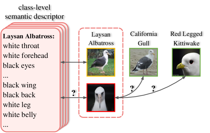
Instead of adopting the commonly-used semantic embedding model [11, 12], we propose a contrastive embedding in our hybrid GZSL framework. The traditional semantic embedding in ZSL relies on a ranking loss, which requires the correct (positive) semantic descriptor to be ranked higher than any of wrong (negative) descriptors with respect to the embedding of a training sample. The semantic embedding methods only utilize the class-wise supervision. In contrastive embedding, we wish to exploit not only the class-wise supervision but also the instance-wise supervision for GZSL, as depicted in Figure 1. Our proposed contrastive embedding learns to discriminate between one positive sample (or semantic descriptor) and a large number of negative samples (or semantic descriptors) from different classes by leveraging the contrastive loss [23, 24, 25]. We evaluate our method on five benchmark datasets, and to the best of our knowledge, our method can outperform the state-of-the-arts on three datasets by a large margin and achieve competitive results on the other two datasets.

Our contributions are three-fold: (1) we propose a hybrid GZSL framework combining the embedding based model and the feature generation based model; (2) we propose a contrastive embedding, which can utilize both the class-wise supervision and the instance-wise supervision, in our hybrid GZSL framework; and (3) we evaluate our GZSL model on five benchmarks and our method can achieve the state-of-the-arts or competitive results on these datasets.

2 Related Work

Zero-shot learning [2, 3] aims to transfer the object recognition model from seen to unseen classes via the shared semantic space, in which both seen and unseen classes have their semantic descriptors. Early ZSL works focus on the conventional ZSL problem. These works typically learn to embed visual samples and the semantic descriptors to an embedding space [11, 7, 26, 12, 27, 28, 29, 13, 30, 31, 32] (e.g. the visual space or the semantic descriptor space). In the embedding space, the visual samples from the same class are supposed to center around the corresponding class-level semantic descriptor. They implement conventional ZSL recognition by searching the nearest semantic descriptor in the embedding space. In the more challenging GZSL scenario, however, embedding-based methods suffer from the seen classes overfitting problem due to the data-imbalance nature of ZSL [10]. To relieve the overfitting problem, some methods [9, 33, 34, 35, 36, 37, 38] have designed new loss functions to balance the predictions between seen and unseen classes. Some other works [39, 40, 41] have regarded GZSL as an out-of-distribution detection problem. Moreover, some researches [42, 43, 44] have introduced the knowledge graph in GZSL to propagate the learned knowledge from seen to unseen classes through the knowledge graph.

To further mitigate the data imbalance problem, feature generation methods learn to complement the visual samples for unseen classes [17, 18, 19, 20, 21, 45, 46, 47]. The feature generation methods first learn a conditional generative model based on such as Variational Autoencoder (VAE) [48] and Generative Adversarial Networks (GAN) [49, 50], conditioned on the semantic descriptors. With the learned generative model, they can synthesize the missing visual examples for unseen classes using the corresponding semantic descriptors. With the real examples from seen classes and the synthesized examples from unseen classes, they can transform the GZSL problem into a standard supervised classification problem and learn a supervised classifier to implement GZSL recognition. Recently, Shen et al. [22] have introduced Generative Flows [51, 52, 53] into zero-shot learning and achieved good performance for GZSL and conventional ZSL.

Though existing methods have achieved great success on GZSL, as discussed before, the original visual feature space lacks the discriminative ability and is suboptimal for GZSL classification. Therefore, we propose a hybrid GZSL framework, integrating a feature generation model with an embedding based model. Inspired by the emerging contrastive representation learning [23, 24, 25, 54, 55], we propose a contrastive embedding model for our hybrid GZSL framework, in which we consider both the instance-wise supervision and the class-wise supervision. In contrast, the traditional semantic embedding for ZSL only utilizes the class-wise supervision. Our hybrid GZSL framework maps the real seen samples and the synthetic unseen samples into a new embedding space, where we learn a supervised classifier, e.g. softmax, as the final GZSL classifier.

3 Contrastive Embedding for GZSL

In this section, we first define the Generalized Zero-Shot Learning (GZSL) problem, before introducing the proposed hybrid GZSL framework and the contrastive embedding in it.

3.1 Problem definition

In ZSL, we have two disjoint sets of classes: $S$ seen classes in $\mathcal{Y}_{s}$ and $U$ unseen classes in $\mathcal{Y}_{u}$, where we have $\mathcal{Y}_{s}\cap\mathcal{Y}_{u}=\varnothing$. Suppose that $N$ labeled instances from seen classes $\mathcal{Y}_{s}$ are provided for training: $\mathcal{D}_{tr}=\{(x_{1},y_{2}),\dots,(x_{N},y_{N})\}$, where $x_{i}\in\mathcal{X}$ denotes the instance and $y_{i}\in\mathcal{Y}_{s}$ is the corresponding seen class label. The test set $\mathcal{D}_{te}=\{x_{N+1},\dots,x_{N+M}\}$ contains $M$ unlabeled instances. In conventional ZSL, the instances in $\mathcal{D}_{te}$ come from unseen classes only. Under the more challenging Generalized Zero-Shot Learning (GZSL) setting, the instances in $\mathcal{D}_{te}$ come from both seen and unseen classes. At the same time, the class-level semantic descriptors of both seen and unseen classes are also provided $\mathcal{A}=\{a_{1},\dots,a_{S},a_{S+1},\dots,a_{S+U}\}$, where the first $S$ semantic descriptors correspond to seen classes in $\mathcal{Y}_{s}$ and the last $U$ semantic descriptors correspond to unseen classes in $\mathcal{Y}_{u}$. We can infer the semantic descriptor $a$ for a labeled instance $x$ from its class label $y$.

Figure 2: Illustration of our proposed hybrid GZSL framework with contrastive embedding (CE-GZSL). We learn an embedding function $E$ that maps the visual samples $x_{i}$ into the embedding space as $h_{i}=E(x_{i})$. We further learn a non-linear projection $H$ to better constrain the embedding space: $z_{i}=H(h_{i})$. We introduce a comparator network $F$ that measures the relevance score between $h_{i}$ and the semantic descriptors. We learn the embedding function with both the instance-level and the class-level supervisions. We integrate the contrastive embedding model with the feature generation model. In the feature generation model, the feature generator $G$ learns to produce visual features based on a semantic descriptor $a$ and a Gaussian noise $\epsilon$; and the discriminator $D$ aims to distinguish the fake visual features from real ones.

3.2 A Hybrid GZSL Framework

Semantic embedding (SE) in conventional ZSL aims to learn an embedding function $E$ that maps a visual feature $x$ into the semantic descriptor space denoted as $E(x)$. The commonly-used semantic embedding methods rely on a structured loss function proposed in [12, 11]. The structured loss requires the embedding of $x$ being closer to the semantic descriptor $a$ of its ground-truth class than the descriptors of other classes, according to the dot-product similarity in the semantic descriptor space. Concretely, the structured loss is formulated as below:

$$\mathcal{L}_{se}^{real}(E)=\mathbb{E}_{p(x,a)}[\max(0,\Delta-a^{\top}E(x)+(a^{\prime})^{\top}E(x))],$$ (1)

where $p(x,a)$ is the empirical distribution of the real training samples of seen classes, $a^{\prime}\neq a$ is a randomly-selected semantic descriptor of other classes, and $\Delta>0$ is a margin parameter to make $E$ more robust.

Semantic embedding methods are less effective in GZSL due to the severe bias towards seen classes. Recently, many feature generation methods [20, 19, 18, 56, 57] have been proposed to synthesize the missing training samples for unseen classes. Feature generation methods learn a conditional generator network $G$ to produce the samples $\tilde{x}=G(a,\epsilon)$ conditioned on a Gaussian noise $\epsilon\sim\mathcal{N}(\mathbf{0},\mathbf{I})$ and a semantic descriptor $a$. In the meanwhile, a discriminator network $D$ is learned together with $G$ to discriminate a real pair $(x,a)$ from a synthetic pair $(\tilde{x},a)$. The feature generator $G$ tries to fool the discriminator $D$ by producing indistinguishable synthetic features. The feature generation methods hope to match the synthetic feature distribution with the real feature distribution in the original feature space. The feature generator network $G$ and the discriminator network $D$ can be learned by optimizing the following adversarial objective:

$$V(G,D)= \mathbb{E}_{p(x,a)}[\log D(x,a)]$$ (2)

$$+\mathbb{E}_{p_{G}(\tilde{x},a)}[\log(1-D(\tilde{x},a))],$$

where $p_{G}(\tilde{x},a)=p_{G}(\tilde{x}|a)p(a)$ is the joint distribution of a synthetic feature and its corresponding semantic descriptor.

The feature generation methods learn to synthesize the visual features in the original feature space. However, in the original feature space, the visual features are usually not well-structured and thus are suboptimal for GZSL classification. In this paper, we propose a hybrid GZSL framework, integrating the embedding model and the feature generation model. In our hybrid GZSL framework, we map both the real features and the synthetic features into an embedding space, where we perform the final GZSL classification. In its simplest form, we just choose the semantic descriptor space as the embedding space and combine the learning objective of semantic embedding defined in Eq. 1 and the objective of feature generation defined in Eq. 2. To map the synthesized features into the embedding space as well, we introduce the following embedding loss for the synthetic features:

$$\mathcal{L}_{se}^{sync}(G,E)=\mathbb{E}_{a}[\max(0,\Delta -a^{\top}E(G(a,\epsilon))$$ (3)

$$+(a^{\prime})^{\top}E(G(a,\epsilon)))].$$

Notably, we formulate $\mathcal{L}_{se}^{sync}(G,E)$ only using the semantic descriptors of seen classes. Therefore, the total loss of our basic hybrid GZSL approach takes the form of

$$\max_{D}\min_{G,E}V(G,D)+\mathcal{L}_{se}^{real}(E)+\mathcal{L}_{se}^{sync}(G,E).$$ (4)

3.3 Contrastive Embedding

Our basic hybrid GZSL framework is based on the traditional semantic embedding model, where only the class-wise supervision is exploited. In this section, we present a new contrastive embedding (CE) model for our hybrid GZSL framework. The contrastive embedding consists of the instance-level contrastive embedding based on the instance-wise supervision and the class-level contrastive embedding based on the class-wise supervision.

Instance-level contrastive embedding

In the embedding space, the embedding of a visual sample $x$ is denoted as $h=E(x)$. For each data point $h_{i}$ embedded from either a real or synthetic seen feature, we set up a $(K+1)$-way classification subproblem to distinguish the unique one positive example $h^{+}$ from total $K$ negative examples $\{h_{1}^{-},\dots,h_{K}^{-}\}$. The positive example $h^{+}$ being randomly selected has the same class label with $h_{i}$, while the class labels of the negative examples are different from $h_{i}$’s class label. Here, we follow the strategy in [58] to add a non-linear projection head $H$ in the embedding space: $z_{i}=H(h_{i})=H(E(x_{i}))$. And we perform the $(K+1)$-way classification on $z_{i}$ to learn the embedding $h_{i}$. Concretely, the cross-entropy loss of this $(K+1)$-way classification problem is calculated as follows:

$$\ell_{ce}^{ins}(z_{i},z^{+})=-\log\frac{\exp{\left(z_{i}^{\top}z^{+}/\tau_{e}\right)}}{\exp{\left(z_{i}^{\top}z^{+}/\tau_{e}\right)}+\sum_{k=1}^{K}\exp{\left(z_{i}^{\top}z_{k}^{-}/\tau_{e}\right)}},$$ (5)

where $\tau_{e}>0$ is the temperature parameter for the instance-level contrastive embedding and $K$ is the number of negative examples. Intuitively, a large $K$ will make the problem in Eq. 5 more difficult. The large number of negative examples encourages the embedding function $E$ to capture the strong discriminative information and structures shared by the samples, real and synthetic, from the same class in the embedding space.

To learn the embedding function $E$, the non-linear projection $H$ and the feature generator network $G$, we calculate the loss function for the instance-level contrastive embedding as the expected loss computed over the randomly selected pairs $z_{i}$ and $z^{+}$ for both the real and synthetic examples, where $z_{i}\neq z^{+}$ but they belong to the same seen class.

$$\mathcal{L}_{ce}^{ins}(G,E,H)=\mathbb{E}_{z_{i},z^{+}}\left[\ell_{ce}^{ins}(z_{i},z^{+})\right].$$ (6)

Class-level contrastive embedding

Analogously, we can formulate a class-level contrastive embedding. Since we do not limit our embedding space to be the semantic descriptor space, we cannot compute the dot-product similarity between an embedded data point and a semantic descriptor directly. Thus, we learn a comparator network $F(h,a)$ that measures the relevance score between an embedding $h$ and a semantic descriptor $a$. With the help of the comparator network $F$, we formulate the class-level contrastive embedding loss for a randomly selected point $h_{i}$ in the embedding space as an $S$-way classification subproblem. The goal of this subproblem is to select the only one correct semantic descriptor from total $S$ semantic descriptors of seen classes. In this problem, the only positive semantic descriptor is the one corresponding to $h_{i}$’s class, while the remaining $S-1$ semantic descriptors from the other classes are treated as the negative semantic descriptors. Similarly, we can calculate the cross-entropy loss of this $S$-way classification problem as below:

$$\ell_{ce}^{cls}(h_{i},a^{+})=-\log\frac{\exp{\left(F(h_{i},a^{+})/\tau_{s}\right)}}{\sum_{s=1}^{S}\exp{\left(F(h_{i},a_{s})/\tau_{s}\right)}},$$ (7)

where $\tau_{s}>0$ is the temperature parameter for the class-level contrastive embedding and $S$ is the number of seen classes. The class-level contrastive embedding relies on the class-wise supervision to strengthen the discriminative ability of the samples in the new embedding space.

We define the following loss function for the class-level contrastive embedding:

$$\mathcal{L}_{ce}^{cls}(G,E,F)=\mathbb{E}_{h_{i},a^{+}}\left[\ell_{ce}^{cls}(h_{i},a^{+})\right],$$ (8)

which is the expected loss over the samples, either real or synthetic, in the new embedding space, and their corresponding semantic descriptor, i.e. the positive descriptor.

Total loss

In our final hybrid GZSL framework, we replace the semantic embedding (SE) model in the basic hybrid framework in Eq. 4 with the proposed contrastive embedding (CE) model. As described above, the contrastive embedding model consists of an instance-level loss function $\mathcal{L}_{ce}^{ins}$ and a class-level loss function $\mathcal{L}_{ce}^{cls}$. Thus, the total loss of our final hybrid GZSL framework with contrastive embedding (CE-GZSL) is formulated as:

$$\max_{D}\min_{G,E,H,F}V(G,D)+\mathcal{L}_{ce}^{ins}(G,E,H)+\mathcal{L}_{ce}^{cls}(G,E,F).$$ (9)

Figure 2 illustrates the whole structure of our method. In our method, we learn a feature generator $G$ (together with a discriminator $D$) to synthesize the missing unseen class features; we learn an embedding function $E$ to embed the samples, both real and synthetic, to a new embedding space, where we conduct the final GZSL classification; to learn a more effective embedding space, we introduce a non-linear projection $H$ in the embedding space which is used to define the instance-level contrastive embedding loss; and to enforce the class-wise supervision, we learn a comparator network $F$ to compare an embedding and a semantic descriptor.

GZSL classification

We first generate the features for each unseen class in the embedding space by composing the feature generator network $G$ and the embedding function $E$: $\tilde{h}_{j}=E(G(a_{u},\epsilon))$, where $u\geq S+1$ and $a_{u}$ is the semantic descriptor of an unseen class. We map the given training features of seen classes in $\mathcal{D}_{tr}$ into the same embedding space as well: $h_{i}=E(x_{i})$. In the end, we utilize the real seen samples and the synthetic unseen samples in the embedding space to train a softmax model as the final GZSL classifier.

4 Experiments

Datasets

We evaluate our method on five benchmark datasets for ZSL: Animals with Attributes 1&2 (AWA1 [2] & AWA2 [16]), Caltech-UCSD Birds-200-2011 (CUB) [59], Oxford Flowers (FLO) [60], and SUN Attribute (SUN) [61]. AWA1 and AWA2 share the same 50 categories and each category is annotated with 85 attributes, which we use as the class-level semantic descriptors. AWA1 contains 30,475 images and AWA2 contains 37,322 images; CUB contains 11,788 images from 200 bird species; FLO contains 8,189 images of 102 fine-grained flower classes; SUN contains 14,340 images from 717 different scenes and each class is annotated with 102 attributes. For the semantic descriptors of CUB and FLO, we adopt the 1024-dimensional class embeddings generated from textual descriptions [62]. We extract the 2,048-dimensional CNN features for all datasets with ResNet-101 [63] pre-trained on ImageNet-1K [1] without finetuning. Moreover, we adopt the Proposed Split (PS) [16] to divide all classes on each dataset into seen and unseen classes.

Evaluation Protocols

We follow the evaluation strategy proposed in  [16]. Under the conventional ZSL scenario, we only evaluate the per-class Top-1 accuracy on unseen classes. Under the GZSL scenario, we evaluate the Top-1 accuracy on seen classes and unseen classes, respectively, denoted as ${S}$ and ${U}$. The performance of GZSL is measured by their harmonic mean: ${H}=2\times{S}\times{U}/({S}+{U})$.

Table 1: Comparisons with the state-of-the-art GZSL methods. $U$ and $S$ are the Top-1 accuracies tested on unseen classes and seen classes, respectively, in GZSL. $H$ is the harmonic mean of $U$ and $S$. The best results are marked in bold.

Method	AWA1			AWA2			CUB			FLO			SUN
	${U}$	${S}$	${H}$	${U}$	${S}$	${H}$	${U}$	${S}$	${H}$	${U}$	${S}$	${H}$	${U}$	${S}$	${H}$
DAZLE [35]	-	-	-	60.3	75.7	67.1	56.7	59.6	58.1	-	-	-	52.3	24.3	33.2
TCN [64]	49.4	76.5	60.0	61.2	65.8	63.4	52.6	52.0	52.3	-	-	-	31.2	37.3	34.0
Li et al. [65]	62.7	77.0	69.1	56.4	81.4	66.7	47.4	47.6	47.5	-	-	-	36.3	42.8	39.3
Zhu et al. [66]	57.3	67.1	61.8	55.3	72.6	62.6	47.0	54.8	50.6	-	-	-	45.3	36.8	40.6
SE-GZSL [19]	56.3	67.8	61.5	58.3	68.1	62.8	41.5	53.3	46.7	-	-	-	40.9	30.5	34.9
f-CLSWGAN [20]	57.9	61.4	59.6	-	-	-	43.7	57.7	49.7	59.0	73.8	65.6	42.6	36.6	39.4
cycle-CLSWGAN [67]	56.9	64.0	60.2	-	-	-	45.7	61.0	52.3	59.2	72.5	65.1	49.4	33.6	40.0
CADA-VAE [68]	57.3	72.8	64.1	55.8	75.0	63.9	51.6	53.5	52.4	-	-	-	47.2	35.7	40.6
f-VAEGAN-D2 [21]	-	-	-	57.6	70.6	63.5	48.4	60.1	53.6	56.8	74.9	64.6	45.1	38.0	41.3
LisGAN [69]	52.6	76.3	62.3	-	-	-	46.5	57.9	51.6	57.7	83.8	68.3	42.9	37.8	40.2
RFF-GZSL [70]	59.8	75.1	66.5	-	-	-	52.6	56.6	54.6	65.2	78.2	71.1	45.7	38.6	41.9
IZF [22]	61.3	80.5	69.6	60.6	77.5	68.0	52.7	68.0	59.4	-	-	-	52.7	57.0	54.8
TF-VAEGAN [71]	-	-	-	59.8	75.1	66.6	52.8	64.7	58.1	62.5	84.1	71.7	45.6	40.7	43.0
Our CE-GZSL	65.3	73.4	69.1	63.1	78.6	70.0	63.9	66.8	65.3	69.0	78.7	73.5	48.8	38.6	43.1

Implementation Details

We implement our method with PyTorch. On all datasets, we set the dimension of the embedding $h$ to 2,048, and set the dimension of the non-linear projection’s output $z$ to 512. The comparator network $F$ is a multi-layer perceptron (MLP) containing a hidden layer with LeakyReLU activation. The comparator network $F$ takes as input the concatenation of an embedding $h$ and a semantic descriptor $a$, and outputs the relevance estimation between them. Our generator $G$ and discriminator $D$ both contain a 4096-unit hidden layer with LeakyReLU activation. We use a random mini-batch size of 4,096 for AWA1 and AWA2, 2,048 for CUB, 3,072 for FLO, and 1,024 for SUN in our method. In the mini-batch, the instances from the same class are positive instances to each other, while the instances from different classes are negative instances to each other. The large batch size ensures a large number of negative instances in our method.

Table 2: Results of conventional ZSL. The first six methods are early conventional ZSL methods and the following ten methods are recent proposed GZSL methods. The best results and the second best results are respectively marked in bold and underlined.

Method	AWA1	AWA2	CUB	FLO	SUN
LATEM [72]	55.1	55.8	49.3	40.4	55.3
DEVISE [11]	54.2	59.7	52.0	45.9	56.5
SJE [12]	65.6	61.9	53.9	53.4	53.7
ALE [7]	59.9	62.5	54.9	48.5	58.1
ESZSL [13]	58.2	58.6	53.9	51.0	54.5
SYNC [73]	54.0	46.6	55.6	-	56.3
DCN [33]	65.2	-	56.2	-	61.8
SP-AEN [74]	58.5	-	55.4	-	59.2
cycle-CLSWGAN [67]	66.3	-	58.4	70.1	60.0
LFGAA [75]	-	68.1	67.6	-	61.5
DLFZRL [76]	71.3	70.3	61.8	-	61.3
Zhu et al. [66]	69.3	70.4	58.5	-	61.5
TCN [64]	70.3	71.2	59.5	-	61.5
f-CLSWGAN [20]	68.2	-	57.3	67.2	60.8
f-VAEGAN-D2 [21]	-	71.1	61.0	67.7	64.7
TF-VAEGAN [71]	-	72.2	64.9	70.8	66.0
Our CE-GZSL	71.0	70.4	77.5	70.6	63.3

Table 3: The effect of the hybrid GZSL framework. ‘Gen’ denotes the feature generation model, ‘SE’ denotes the semantic embedding model, and ‘+’ denotes their hybrid combination. We evaluate these methods in three spaces: visual space (‘V’), semantic space (‘S’), and a new embedding space (‘E’).

Method	Space	AWA1			AWA2			CUB			FLO			SUN
		${U}$	${S}$	${H}$	${U}$	${S}$	${H}$	${U}$	${S}$	${H}$	${U}$	${S}$	${H}$	${U}$	${S}$	${H}$
Gen	V	53.0	67.7	59.5	56.9	61.6	59.2	54.1	59.4	56.6	57.5	75.5	65.3	43.0	37.2	39.9
SE	S	21.8	55.7	31.3	21.1	59.9	31.2	36.3	44.2	39.9	24.0	62.6	34.7	19.0	27.1	22.4
Gen+SE (basic)	S	50.5	62.5	55.9	50.6	64.3	56.6	52.2	59.3	55.5	53.2	78.6	63.4	35.1	23.3	28.0
Gen+SE	E	63.1	71.3	66.9	61.7	75.6	67.9	61.1	65.3	63.1	66.1	72.2	69.0	47.9	36.1	41.1

Table 4: The effect of different embedding models (E-M) and different spaces in the hybrid GZSL framework. All the methods here are combined with the feature generation model. ‘SE’ denotes the semantic embedding model and ‘CE’ denotes our contrastive embedding model. We evaluate the embedding models in two embedding spaces: semantic descriptor space (S) and the new embedding space (E).

Space	E-M	AWA1			AWA2			CUB			FLO			SUN
		${U}$	${S}$	${H}$	${U}$	${S}$	${H}$	${U}$	${S}$	${H}$	${U}$	${S}$	${H}$	${U}$	${S}$	${H}$
V	None	53.0	67.7	59.5	56.9	61.6	59.2	54.1	59.4	56.6	57.5	75.5	65.3	43.0	37.2	39.9
S	SE (basic)	50.5	62.5	55.9	50.6	64.3	56.6	52.2	59.3	55.5	53.2	78.6	63.4	35.1	23.3	28.0
	CE	55.0	65.9	59.9	55.8	70.7	62.4	61.5	67.4	64.3	56.1	78.9	65.5	37.6	30.4	33.6
E	SE	63.1	71.3	66.9	61.7	75.6	67.9	61.1	65.3	63.1	66.1	72.2	69.0	47.9	36.1	41.1
	CE (Our CE-GZSL)	65.3	73.4	69.1	63.1	78.6	70.0	63.9	66.8	65.3	69.0	78.7	73.5	48.8	38.6	43.1

Table 5: Evaluation of each part of our contrastive embedding (CE) model in the hybrid GZSL framework. ‘Our CE-GZSL’ denotes the whole CE model.

Method	AWA1			AWA2			CUB			FLO			SUN
	${U}$	${S}$	${H}$	${U}$	${S}$	${H}$	${U}$	${S}$	${H}$	${U}$	${S}$	${H}$	${U}$	${S}$	${H}$
$V(G,D)+\mathcal{L}_{ce}^{ins}(G,E,H)$	64.7	71.3	67.8	64.4	72.3	68.1	58.8	66.5	62.4	62.9	77.3	69.4	49.0	32.0	38.7
$V(G,D)+\mathcal{L}_{ce}^{cls}(G,E,F)$	63.6	72.0	67.5	61.2	79.3	69.1	62.7	63.3	63.0	66.0	79.7	72.2	49.1	37.4	42.4
Our CE-GZSL	65.3	73.4	69.1	63.1	78.6	70.0	63.9	66.8	65.3	69.0	78.7	73.5	48.8	38.6	43.1

4.1 Comparison with SOTA

In Table 1, we compare our CE-GZSL method with the state-of-the-art GZSL methods. Our method achieves the best $U$ on four datasets and achieves the best $H$ on AWA2, CUB, and FLO. Notably, on CUB, our CE-GZSL is the first one that obtains the performances $>60.0$ on $U$ and $H$ among the state-of-the-art GZSL methods. Especially, our hybrid GZSL method integrating with the simplest generative model still achieves competitive results compared with IZF [22], which is based on the most advanced generative model in GZSL. Our CE-GZSL achieves the second best $H$ on AWA1 and SUN, and is only lower than IZF [22], and on the other three datasets our CE-GZSL outperforms IZF [22] by a large margin. In Table 2, we report the results of our CE-GZSL under the conventional ZSL scenario. We compare our method with sixteen methods, in which six of them are traditional methods and ten of them are the recent methods. Our method is still competitive in conventional ZSL. Our method performs the best on CUB and the second best on AWA1 and FLO in the conventional ZSL scenario. Specifically, on CUB, our method also achieves an excellent performance, and our CE-GZSL is the only method that can achieve the performance $>70.0$ under conventional ZSL among the ten recent methods.

4.2 Component Analysis

In Table 3, we illustrate the effectiveness of the hybrid strategy for GZSL. First, we respectively evaluate the performances of the single feature generation model (Gen) and the single semantic embedding model (SE). We evaluate them in their original space: visual space (V) for ‘Gen’ and semantic space (S) for ‘SE’. ‘Gen+SE (basic)’ denotes that we simply combine the feature generation model with the semantic embedding model and learn a softmax classifier in semantic space, corresponding to the basic hybrid GZSL approach defined in Eq. 4. Moreover, we introduce a new embedding space (E) in the hybrid GZSL method, which leads to the increased performance. The results show that the hybrid GZSL strategy is effective, and the new embedding space is better than the semantic space.

In Table 4, we investigate the effect of different spaces and different embedding models in the hybrid GZSL framework. We integrate the feature generation model with two different embedding models: semantic embedding (SE) (i.e. the ranking loss method) and our contrastive embedding (CE). And we evaluate the semantic descriptor space (S) and the new embedding space (E), in which we conduct the final GZSL classification. Firstly, we evaluate the same embedding model on different embedding spaces: the results of ‘SE’ on the new embedding space performs much better than ‘SE (basic)’ on the semantic space; and ‘CE (Our CE-GZSL)’ on the new embedding space also performs better than ‘CE’ on the semantic descriptor space. This demonstrates that the new embedding space is much more effective than the original semantic space in our hybrid framework. Afterward, we compare the results on the same embedding space but using different embedding models: ‘SE’ corresponds to the ranking loss form in Eq. 3 and ‘CE’ corresponds to contrastive form in Eq. 7. Our proposed ‘CE’ can always outperform ‘SE’, no matter in the semantic descriptor space or in the new embedding space. This illustrates that our contrastive embedding (CE) benefits from the instance-wise supervision which is neglected in the traditional semantic embedding (SE).

Moreover, in Table 5, we respectively evaluate the instance-level supervision and the class-level supervision in our contrastive embedding model. Concretely, to evaluate the instance-level supervision, we remove the class-level supervision $\mathcal{L}_{ce}^{cls}(G,E,F)$ in Eq. 9 and only optimize $V(G,D)+\mathcal{L}_{ce}^{ins}(G,E,H)$ to learn our contrastive embedding model. In the same way, we evaluate the class-level supervision by optimizing $V(G,D)+\mathcal{L}_{ce}^{cls}(G,E,F)$. As shown in Table 5, when using either the instance-level CE or the class-level CE, our result is still competitive compared with the state-of-the-art GZSL methods. When considering both the instance-level supervision and the class-level supervisions, our method achieves the improvements on $U$ and $S$, leading to the better $H$ results. This means that our method benefits from the combination of the instance-level supervision and the class-level supervision.

(a) AWA1

(b) AWA2

(c) CUB

(d) FLO

(e) SUN

Figure 3: The GZSL results with respect to different numbers of the synthesized samples for each unseen class.

(a) AWA1

(b) AWA2

(c) CUB

(d) FLO

(e) SUN

Figure 4: The results of harmonic mean $H$ in GZSL with respect to different temperature parameters $\tau_{e}$ and $\tau_{s}$.

Table 6: Our CE-GZSL results with respect to different dimensions of the embedding $h$. $U$ and $S$ are the Top-1 accuracies tested on unseen classes and seen classes, respectively, in GZSL. $H$ is the harmonic mean of $U$ and $S$.

Dimension	AWA1			AWA2			CUB			FLO			SUN
	${U}$	${S}$	${H}$	${U}$	${S}$	${H}$	${U}$	${S}$	${H}$	${U}$	${S}$	${H}$	${U}$	${S}$	${H}$
256	52.9	53.9	53.3	56.6	71.8	63.3	62.5	51.5	62.0	63.0	47.2	53.9	46.7	28.9	35.7
512	65.0	55.7	60.0	60.7	75.4	67.3	62.2	66.1	64.1	68.1	58.0	62.6	50.1	33.6	40.2
1,024	65.7	65.1	65.4	61.9	77.9	69.0	62.2	66.5	64.3	63.2	78.0	69.8	48.7	36.7	41.9
2,048	64.9	73.9	69.0	63.1	78.6	70.0	63.9	66.8	65.3	69.0	78.7	73.5	48.8	38.6	43.1
4,096	62.9	76.4	69.0	66.0	74.5	70.0	63.0	67.6	65.2	68.5	80.3	73.9	45.6	39.0	42.1

4.3 Hyper-Parameter Analysis

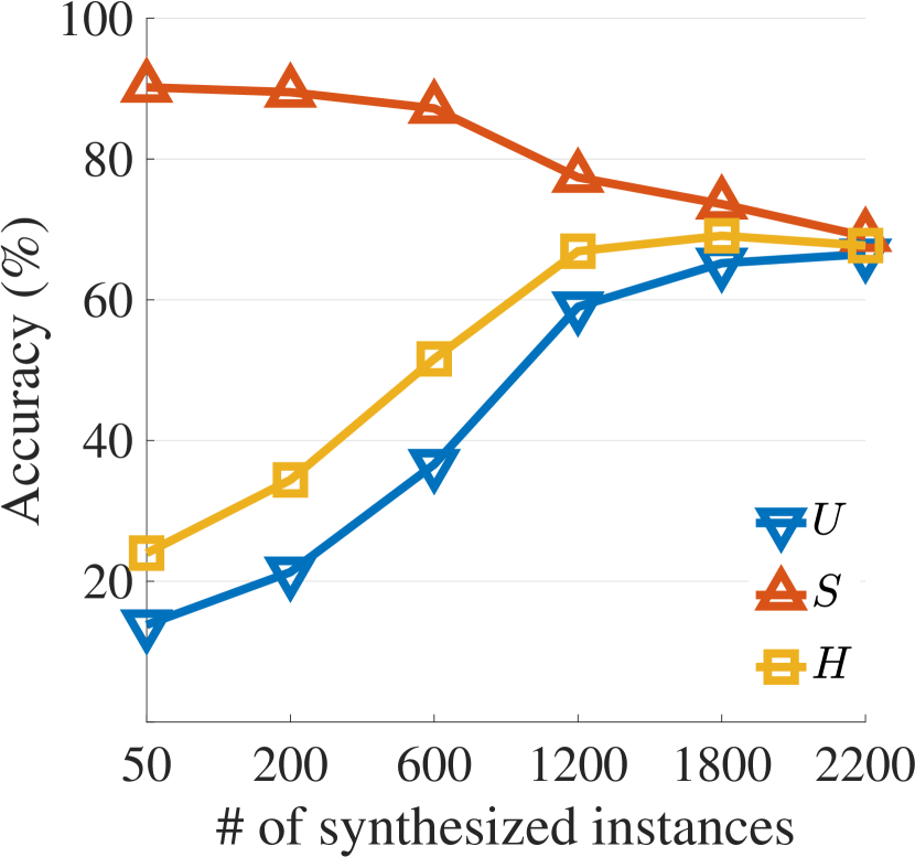
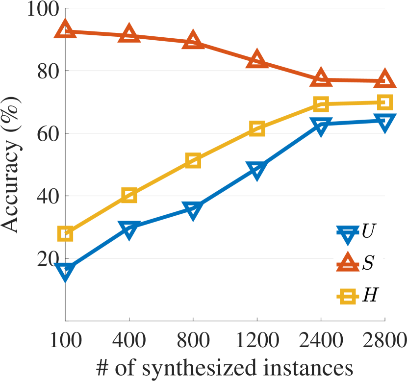
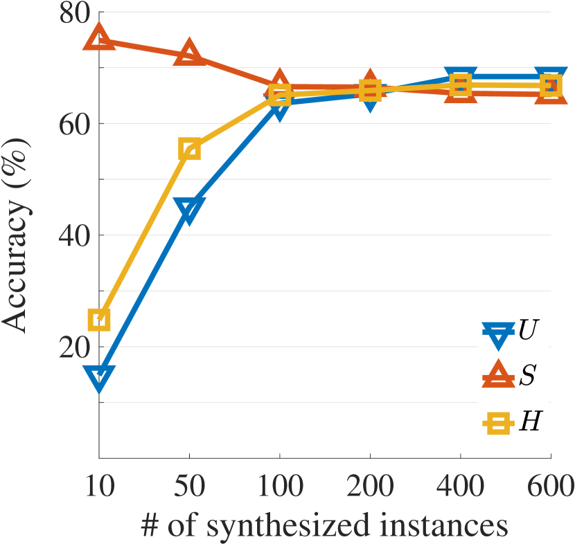
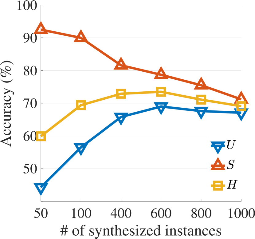
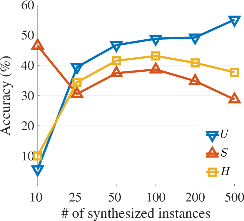
We evaluate the effect of different numbers of synthesized instances per unseen classes as shown in Figure 3. The performances on five datasets increase along with the number of synthesized examples, which shows the data-imbalance problem has been relieved by the generation model in our hybrid GZSL framework. Our method achieves the best results on AWA1, AWA2, CUB, FLO, and SUN when we synthesize 1,800, 2,400, 300, 600, and 100 examples per unseen classes, respectively.

Table 7: The effect of different numbers of positive and negative samples in a mini-batch on AWA1. ‘$P$’ and ‘$K$ denote the numbers of positive examples and negative examples in the mini-batch, respectively.

$P$	$K$	${U}$	${S}$	${H}$
1	50	57.5	74.6	64.9
1	100	59.0	73.2	65.3
1	500	63.1	70.6	66.7
1	1,000	61.8	70.9	66.0
1	2,000	60.9	73.5	66.6
1	4,000	61.5	74.7	67.4
30	50	61.8	72.6	66.8
30	100	61.9	73.1	67.0
30	500	64.2	72.3	68.0
30	1,000	63.5	72.8	67.9
30	2,000	63.7	73.4	68.2
30	4,000	62.4	73.0	67.3
random batch (4,096)		65.3	73.4	69.1

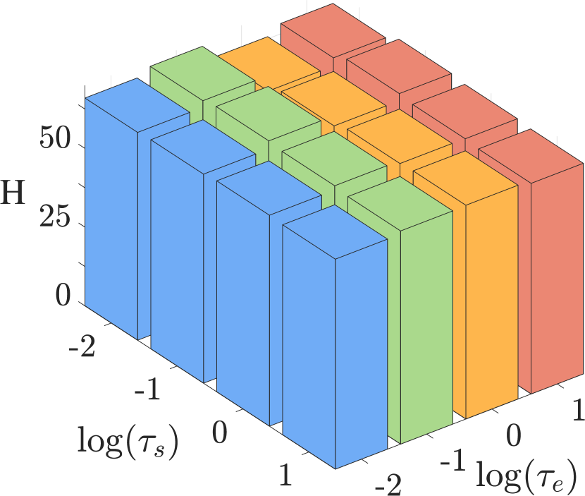
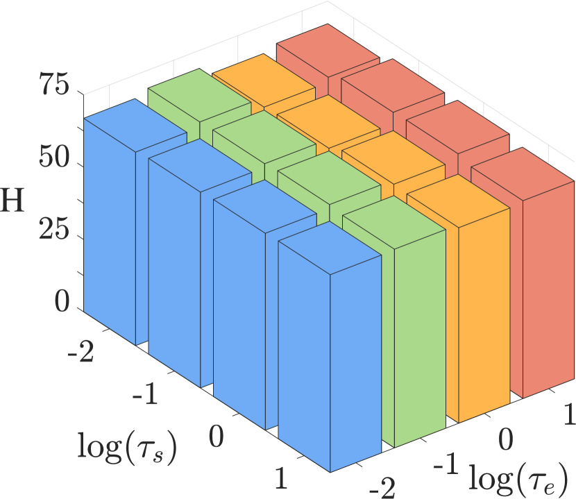
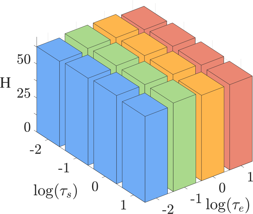
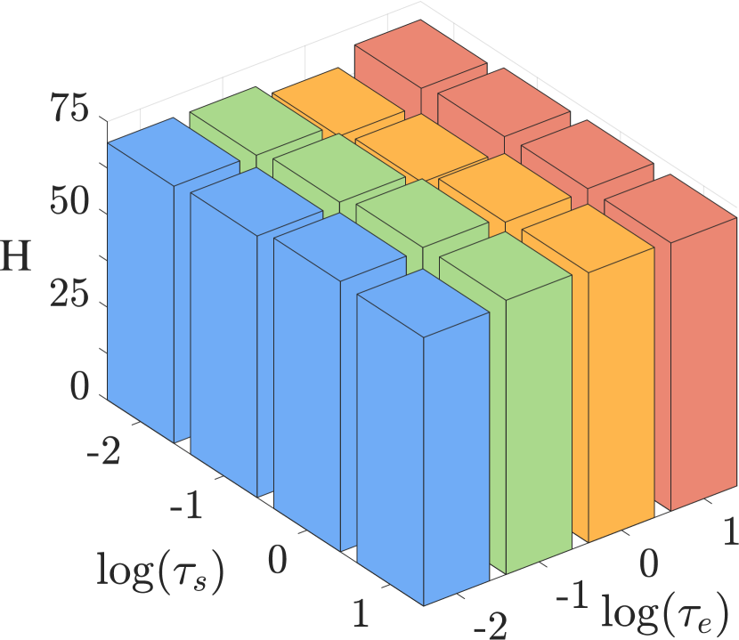
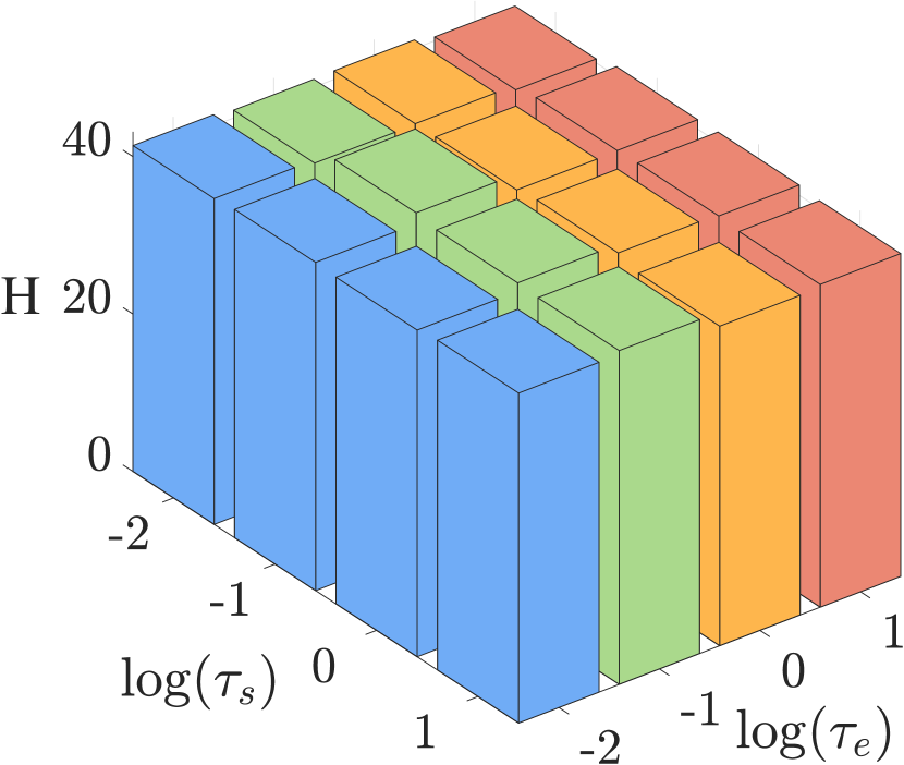
Next, we evaluate the influence of the temperature parameters, $\tau_{e}$ and $\tau_{s}$, in the contrastive embedding model. We cross-validate $\tau_{e}$ and $\tau_{s}$ in $[0.01,0.1,1.0,10.0]$ and plot the $H$ values with respect to different $\tau_{e}$ and $\tau_{s}$, as shown in Figure 4. With the different $\tau_{e}$ and $\tau_{s}$ values, the $H$ results on different datasets change slightly, indicating that our method is robust to the temperature parameters. On AWA1, CUB and SUN, our method achieves the best results when $\tau_{e}=0.1$ and $\tau_{s}=0.1$. On AWA2, our method achieves the best result when $\tau_{e}=10.0$ and $\tau_{s}=1.0$. On FLO, our method achieves the best result when $\tau_{e}=0.1$ and $\tau_{s}=1.0$.

In Table 6, we report the results of our hybrid GZSL with contrastive embedding (CE-GZSL) with respect to different dimensions of the embedding $h$. On each of the datasets, as the dimension of the embedding $h$ grows, the performance of our CE-GZSL improves significantly. However, a high dimensional embedding space will inevitably increase the computational burden. Thus, in our experiments, we set the dimension of the embedding $h$ to 2,048 in order to achieve a trade-off between performance and computational cost.

We further evaluate the effect of the numbers of positive and negative examples in the mini-batch. In a mini-batch, we sample $P$ positive examples and $K$ negative examples for a given example. We report the results on AWA1 in Table 7. We can observe that our method benefits from more positive examples and more negative examples. We find that using a large random batch (4,096) without a hand-crafted designed sampling strategy leads to the best results. The reason is that a large batch will contain enough positive examples and negative examples.

5 Conclusion

In this paper, we have proposed a hybrid GZSL framework, integrating an embedding model and a generation model. The proposed hybrid GZSL framework maps the real and synthetic visual samples into an embedding space, where we can train a supervised recognition model as the final GZSL classifier. Specifically, we have proposed a contrastive embedding model in our hybrid GZSL framework. Our contrastive embedding model can leverage not only the class-wise supervision but also the instance-wise supervision. The latter is usually neglected in existing GZSL researches. The experiments show that our hybrid GZSL framework with contrastive embedding (CE-GZSL) has achieved the state-of-the-arts on three benchmark datasets and achieved the second-best on two datasets.

References

- [1] A. Krizhevsky, I. Sutskever, and G. E. Hinton, “Imagenet classification with deep convolutional neural networks,” in NIPS, 2012.
- [2] C. H. Lampert, H. Nickisch, and S. Harmeling, “Learning to detect unseen object classes by between-class attribute transfer,” in CVPR, 2009.
- [3] M. Palatucci, D. Pomerleau, G. E. Hinton, and T. M. Mitchell, “Zero-shot learning with semantic output codes,” in NIPS, 2009.
- [4] A. Farhadi, I. Endres, D. Hoiem, and D. Forsyth, “Describing objects by their attributes,” in CVPR, 2009.
- [5] T. Mikolov, K. Chen, G. Corrado, and J. Dean, “Efficient estimation of word representations in vector space,” arXiv preprint arXiv:1301.3781, 2013.
- [6] T. Mikolov, I. Sutskever, K. Chen, G. S. Corrado, and J. Dean, “Distributed representations of words and phrases and their compositionality,” in NIPS, 2013.
- [7] Z. Akata, F. Perronnin, Z. Harchaoui, and C. Schmid, “Label-embedding for attribute-based classification,” in CVPR, 2013.
- [8] R. Socher, M. Ganjoo, C. D. Manning, and A. Ng, “Zero-shot learning through cross-modal transfer,” in NIPS, 2013.
- [9] W.-L. Chao, S. Changpinyo, B. Gong, and F. Sha, “An empirical study and analysis of generalized zero-shot learning for object recognition in the wild,” in ECCV, 2016.
- [10] Y. Xian, B. Schiele, and Z. Akata, “Zero-shot learning-the good, the bad and the ugly,” in CVPR, 2017.
- [11] A. Frome, G. S. Corrado, J. Shlens, S. Bengio, J. Dean, T. Mikolov et al., “Devise: A deep visual-semantic embedding model,” in NIPS, 2013.
- [12] Z. Akata, S. Reed, D. Walter, H. Lee, and B. Schiele, “Evaluation of output embeddings for fine-grained image classification,” in CVPR, 2015.
- [13] B. Romera-Paredes and P. Torr, “An embarrassingly simple approach to zero-shot learning,” in ICML, 2015.
- [14] Z. Zhang and V. Saligrama, “Zero-shot learning via semantic similarity embedding,” in CVPR, 2015.
- [15] Z. Fu, T. Xiang, E. Kodirov, and S. Gong, “Zero-shot learning on semantic class prototype graph,” TPAMI, 2017.
- [16] Y. Xian, C. H. Lampert, B. Schiele, and Z. Akata, “Zero-shot learning-a comprehensive evaluation of the good, the bad and the ugly,” TPAMI, 2018.
- [17] M. Bucher, S. Herbin, and F. Jurie, “Generating visual representations for zero-shot classification,” in ICCV, 2017.
- [18] A. Mishra, S. Krishna Reddy, A. Mittal, and H. A. Murthy, “A generative model for zero shot learning using conditional variational autoencoders,” in CVPR, 2018.
- [19] V. Kumar Verma, G. Arora, A. Mishra, and P. Rai, “Generalized zero-shot learning via synthesized examples,” in CVPR, 2018.
- [20] Y. Xian, T. Lorenz, B. Schiele, and Z. Akata, “Feature generating networks for zero-shot learning,” in CVPR, 2018.
- [21] Y. Xian, S. Sharma, B. Schiele, and Z. Akata, “f-vaegan-d2: A feature generating framework for any-shot learning,” in CVPR, 2019.
- [22] Y. Shen, J. Qin, L. Huang, F. Zhu, and L. Shao, “Invertible zero-shot recognition flows,” in ECCV, 2020.
- [23] M. Gutmann and A. Hyvärinen, “Noise-contrastive estimation: A new estimation principle for unnormalized statistical models,” in AISTATS, 2010.
- [24] A. v. d. Oord, Y. Li, and O. Vinyals, “Representation learning with contrastive predictive coding,” arXiv preprint arXiv:1807.03748, 2018.
- [25] Z. Wu, Y. Xiong, S. X. Yu, and D. Lin, “Unsupervised feature learning via non-parametric instance discrimination,” in CVPR, 2018.
- [26] Y. Fu, T. M. Hospedales, T. Xiang, Z. Fu, and S. Gong, “Transductive multi-view embedding for zero-shot recognition and annotation,” in ECCV, 2014.
- [27] Z. Fu, T. Xiang, E. Kodirov, and S. Gong, “Zero-shot object recognition by semantic manifold distance,” in CVPR, 2015.
- [28] E. Kodirov, T. Xiang, Z. Fu, and S. Gong, “Unsupervised domain adaptation for zero-shot learning,” in ICCV, 2015, pp. 2452–2460.
- [29] Y. Fu, T. M. Hospedales, T. Xiang, and S. Gong, “Transductive multi-view zero-shot learning,” TPAMI, 2015.
- [30] M. Bucher, S. Herbin, and F. Jurie, “Improving semantic embedding consistency by metric learning for zero-shot classiffication,” in ECCV, 2016.
- [31] E. Kodirov, T. Xiang, and S. Gong, “Semantic autoencoder for zero-shot learning,” in CVPR, 2017.
- [32] Y. L. Cacheux, H. L. Borgne, and M. Crucianu, “Modeling inter and intra-class relations in the triplet loss for zero-shot learning,” in ICCV, 2019.
- [33] S. Liu, M. Long, J. Wang, and M. I. Jordan, “Generalized zero-shot learning with deep calibration network,” in NeurIPS, 2018.
- [34] Y. Annadani and S. Biswas, “Preserving semantic relations for zero-shot learning,” in CVPR, 2018.
- [35] D. Huynh and E. Elhamifar, “Fine-grained generalized zero-shot learning via dense attribute-based attention,” in CVPR, 2020.
- [36] G.-S. Xie, L. Liu, X. Jin, F. Zhu, Z. Zhang, J. Qin, Y. Yao, and L. Shao, “Attentive region embedding network for zero-shot learning,” in CVPR, 2019.
- [37] G.-S. Xie, L. Liu, F. Zhu, F. Zhao, Z. Zhang, Y. Yao, J. Qin, and L. Shao, “Region graph embedding network for zero-shot learning,” in ECCV, 2020.
- [38] S. Min, H. Yao, H. Xie, C. Wang, Z.-J. Zha, and Y. Zhang, “Domain-aware visual bias eliminating for generalized zero-shot learning,” in CVPR, 2020.
- [39] D. Mandal, S. Narayan, S. K. Dwivedi, V. Gupta, S. Ahmed, F. S. Khan, and L. Shao, “Out-of-distribution detection for generalized zero-shot action recognition,” in CVPR, 2019.
- [40] R. Keshari, R. Singh, and M. Vatsa, “Generalized zero-shot learning via over-complete distribution,” in CVPR, 2020.
- [41] X. Chen, X. Lan, F. Sun, and N. Zheng, “A boundary based out-of-distribution classifier for generalized zero-shot learning,” in ECCV, 2020.
- [42] C.-W. Lee, W. Fang, C.-K. Yeh, and Y.-C. Frank Wang, “Multi-label zero-shot learning with structured knowledge graphs,” in CVPR, 2018.
- [43] X. Wang, Y. Ye, and A. Gupta, “Zero-shot recognition via semantic embeddings and knowledge graphs,” in CVPR, 2018.
- [44] S. Liu, J. Chen, L. Pan, C.-W. Ngo, T.-S. Chua, and Y.-G. Jiang, “Hyperbolic visual embedding learning for zero-shot recognition,” in CVPR, 2020.
- [45] A. Paul, N. C. Krishnan, and P. Munjal, “Semantically aligned bias reducing zero shot learning,” in CVPR, 2019.
- [46] M. B. Sariyildiz and R. G. Cinbis, “Gradient matching generative networks for zero-shot learning,” in CVPR, 2019.
- [47] M. R. Vyas, H. Venkateswara, and S. Panchanathan, “Leveraging seen and unseen semantic relationships for generative zero-shot learning,” in ECCV, 2020.
- [48] D. P. Kingma and M. Welling, “Auto-encoding variational bayes,” arXiv preprint arXiv:1312.6114, 2013.
- [49] I. Goodfellow, J. Pouget-Abadie, M. Mirza, B. Xu, D. Warde-Farley, S. Ozair, A. Courville, and Y. Bengio, “Generative adversarial nets,” in NIPS, 2014.
- [50] M. Arjovsky, S. Chintala, and L. Bottou, “Wasserstein gan,” arXiv preprint arXiv:1701.07875, 2017.
- [51] L. Dinh, D. Krueger, and Y. Bengio, “Nice: Non-linear independent components estimation,” arXiv preprint arXiv:1410.8516, 2014.
- [52] L. Dinh, J. Sohl-Dickstein, and S. Bengio, “Density estimation using real nvp,” arXiv preprint arXiv:1605.08803, 2016.
- [53] D. P. Kingma and P. Dhariwal, “Glow: Generative flow with invertible 1x1 convolutions,” in NeurIPS, 2018.
- [54] K. He, H. Fan, Y. Wu, S. Xie, and R. Girshick, “Momentum contrast for unsupervised visual representation learning,” in CVPR, 2020.
- [55] P. Khosla, P. Teterwak, C. Wang, A. Sarna, Y. Tian, P. Isola, A. Maschinot, C. Liu, and D. Krishnan, “Supervised contrastive learning,” in NeurIPS, 2020.
- [56] H. Huang, C. Wang, P. S. Yu, and C.-D. Wang, “Generative dual adversarial network for generalized zero-shot learning,” in CVPR, 2019.
- [57] Y. Atzmon and G. Chechik, “Adaptive confidence smoothing for generalized zero-shot learning,” in CVPR, 2019.
- [58] T. Chen, S. Kornblith, M. Norouzi, and G. Hinton, “A simple framework for contrastive learning of visual representations,” in ICML, 2020.
- [59] C. Wah, S. Branson, P. Welinder, P. Perona, and S. Belongie, “The caltech-ucsd birds-200-2011 dataset,” 2011.
- [60] M.-E. Nilsback and A. Zisserman, “Automated flower classification over a large number of classes,” in ICCVGI, 2008.
- [61] G. Patterson and J. Hays, “Sun attribute database: Discovering, annotating, and recognizing scene attributes,” in CVPR, 2012.
- [62] S. Reed, Z. Akata, H. Lee, and B. Schiele, “Learning deep representations of fine-grained visual descriptions,” in CVPR, 2016.
- [63] K. He, X. Zhang, S. Ren, and J. Sun, “Deep residual learning for image recognition,” in CVPR, 2016.
- [64] H. Jiang, R. Wang, S. Shan, and X. Chen, “Transferable contrastive network for generalized zero-shot learning,” in ICCV, 2019.
- [65] K. Li, M. R. Min, and Y. Fu, “Rethinking zero-shot learning: A conditional visual classification perspective,” in ICCV, 2019.
- [66] Y. Zhu, J. Xie, B. Liu, and A. Elgammal, “Learning feature-to-feature translator by alternating back-propagation for generative zero-shot learning,” in ICCV, 2019.
- [67] R. Felix, V. B. Kumar, I. Reid, and G. Carneiro, “Multi-modal cycle-consistent generalized zero-shot learning,” in ECCV, 2018.
- [68] E. Schonfeld, S. Ebrahimi, S. Sinha, T. Darrell, and Z. Akata, “Generalized zero-and few-shot learning via aligned variational autoencoders,” in CVPR, 2019.
- [69] J. Li, M. Jing, K. Lu, Z. Ding, L. Zhu, and Z. Huang, “Leveraging the invariant side of generative zero-shot learning,” in CVPR, 2019.
- [70] Z. Han, Z. Fu, and J. Yang, “Learning the redundancy-free features for generalized zero-shot object recognition,” in CVPR, 2020.
- [71] S. Narayan, A. Gupta, F. S. Khan, C. G. Snoek, and L. Shao, “Latent embedding feedback and discriminative features for zero-shot classification,” in ECCV, 2020.
- [72] Y. Xian, Z. Akata, G. Sharma, Q. Nguyen, M. Hein, and B. Schiele, “Latent embeddings for zero-shot classification,” in CVPR, 2016.
- [73] S. Changpinyo, W.-L. Chao, B. Gong, and F. Sha, “Synthesized classifiers for zero-shot learning,” in CVPR, 2016.
- [74] L. Chen, H. Zhang, J. Xiao, W. Liu, and S.-F. Chang, “Zero-shot visual recognition using semantics-preserving adversarial embedding networks,” in CVPR, 2018.
- [75] Y. Liu, J. Guo, D. Cai, and X. He, “Attribute attention for semantic disambiguation in zero-shot learning,” in ICCV, 2019.
- [76] B. Tong, C. Wang, M. Klinkigt, Y. Kobayashi, and Y. Nonaka, “Hierarchical disentanglement of discriminative latent features for zero-shot learning,” in CVPR, 2019.