CeBiB — Center for Biotechnology and Bioengineering, Chile and Dept. of Computer Science, University of Chile, Chiledustin.cobas@gmail.comhttps://orcid.org/0000-0001-6081-694XANID/Scholarship Program/DOCTORADO BECAS CHILE/2020-21200906, Chile.CeBiB — Center for Biotechnology and Bioengineering, Chile and Dalhousie University, Canadatravis.gagie@gmail.comhttps://orcid.org/0000-0003-3689-327XFunded by NSERC Discovery Grant RGPIN-07185-2020. CeBiB — Center for Biotechnology and Bioengineering, Chile and Dept. of Computer Science, University of Chile, Chile and http://www.dcc.uchile.cl/gnavarro gnavarro@dcc.uchile.clhttps://orcid.org/0000-0002-2286-741XFondecyt grant 1-200038, ANID, Chile. \CopyrightDustin Cobas and Travis Gagie and Gonzalo Navarro \ccsdesc[500]Theory of computation Pattern matching
Acknowledgements.
Funded with Basal Funds FB0001, ANID, Chile.\hideLIPIcs\EventLongTitle32nd Annual Symposium on Combinatorial Pattern Matching (CPM 2021) \EventShortTitleCPM 2021 \EventAcronymCPM \EventYear2021A Fast and Small Subsampled R-index
Abstract
The r-index (Gagie et al., JACM 2020) represented a breakthrough in compressed indexing of repetitive text collections, outperforming its alternatives by orders of magnitude. Its space usage, where is the number of runs in the Burrows-Wheeler Transform of the text, is however larger than Lempel-Ziv and grammar-based indexes, and makes it uninteresting in various real-life scenarios of milder repetitiveness. In this paper we introduce the sr-index, a variant that limits the space to for a text of length and a given parameter , at the expense of multiplying by the time per occurrence reported. The sr-index is obtained by carefully subsampling the text positions indexed by the r-index, in a way that we prove is still able to support pattern matching with guaranteed performance. Our experiments demonstrate that the sr-index sharply outperforms virtually every other compressed index on repetitive texts, both in time and space, even matching the performance of the r-index while using 1.5–3.0 times less space. Only some Lempel-Ziv-based indexes achieve better compression than the sr-index, using about half the space, but they are an order of magnitude slower.
keywords:
Pattern matching, r-index, compressed text indexing, repetitive text collectionscategory:
\relatedversion1 Introduction
The rapid surge of massive repetitive text collections, like genome and sequence read sets and versioned document and software repositories, has raised the interest in text indexing techniques that exploit repetitiveness to obtain orders-of-magnitude space reductions, while supporting pattern matching directly on the compressed text representations [10, 21].
Traditional compressed indexes rely on statistical compression [22], but this is ineffective to capture repetitiveness [15]. A new wave of repetitiveness-aware indexes [21] build on other compression mechanisms like Lempel-Ziv [16] or grammar compression [14]. A particularly useful index of this kind is the rlfm-index [18, 19], because it emulates the classical suffix array [20] and this simplifies translating suffix-array based algorithms to run on it [17].
The rlfm-index represents the Burrows-Wheeler Transform () [3] of the text in run-length compressed form, because the number of maximal equal-letter runs in the is known to be small on repetitive texts. A problem with the rlfm-index is that, although it can count the number of occurrences of a pattern using space, it needs to sample the text at every th position, for a parameter , in order to locate each of those occurrences in time proportional to . The additional space incurred on a text of length ruins the compression on very repetitive collections, where . The recent r-index [11] closed the long-standing problem of efficiently locating the occurrences within space, offering pattern matching time orders of magnitude faster than previous repetitiveness-aware indexes.
In terms of space, however, the r-index is considerably larger than Lempel-Ziv based indexes of size , where is the number of phrases in the Lempel-Ziv parse. Gagie et al. [11] show that, on extremely repetitive text collections where –, is around and the r-index size is – bits per symbol (bps), about twice that of the lz-index [15], a baseline Lempel-Ziv based index. However, degrades faster than as repetitiveness drops: in an experiment on bacterial genomes in the same article, where , the r-index space approaches bps, times that of the lz-index; also approaches . Experiments on other datasets show that the r-index tends to be considerably larger [23, 5, 6, 1].111The measurements in the article [1] are not correct. Indeed, in some realistic cases can be over 1,500, but in most cases it is well below: 40–160 on versioned software and document collections and fully assembled human chromosomes, 7.5–50 on virus and bacterial genomes (with in the range –), and 4–9 on sequencing reads; see Section 5. An r-index on such a small ratio easily becomes larger than the plain sequence data.
In this paper we tackle the problem of the (relatively) large space usage of the r-index. This index manages to locate the pattern occurrences by sampling text positions (corresponding to the ends of runs). We show that one can remove some carefully chosen samples so that, given a parameter , the index stores only samples while its locating machinery can still be used to guarantee that every pattern occurrence is located within steps. We call the resulting index the subsampled r-index, or sr-index. The worst-case time to locate the occurrences of a pattern of length on an alphabet of size then rises from in the implemented r-index to in the sr-index, which matches the search cost of the rlfm-index.
The sr-index can then be seen as a hybrid between the r-index (matching it when ) and the rlfm-index (obtaining its time with less space; the spaces become similar when repetitiveness drops). In practice, however, the sr-index performs much better than both on repetitive texts, sharply dominating the rlfm-index, the best grammar-based index [5], and in most cases the lz-index, both in space and time. The sr-index can also get as fast as the r-index while using – times less space. Its only remaining competitor is a hybrid between a Lempel-Ziv based and a statistical index [7]. This index can use up to half the space of the sr-index, but it is an order of magnitude slower. Overall, the sr-index stays orders of magnitude faster than all the alternatives while using practical amounts of space in a wide range of repetitiveness scenarios.
2 Background
The suffix array [20] of a string over alphabet is a permutation of the starting positions of all the suffixes of in lexicographic order, for all . The suffix array can be binary searched in time to obtain the range of all the suffixes prefixed by a search pattern (which then occurs times in ). Once they are counted (i.e., their suffix array range is determined), those occurrences are located in time by simply listing their starting positions, . The suffix array can then be stored in bits (plus the bits to store ) and searches for in in total time .
Compressed suffix arrays (s) [22] are space-efficient representations of both the suffix array () and the text (). They can find the interval corresponding to in time and access any cell in time , so they can be used to search for in time . Most s need to store sampled values to compute any in order to support the locate operation, inducing the tradeoff of using extra bits to obtain time proportional to a parameter .
The Burrows-Wheeler Transform [3] of is a permutation of defined as (and if ), which boosts the compressibility of . The fm-index [8, 9] is a that represents and within the statistical entropy of , by exploiting the connection between the and . For counting, the fm-index resorts to backward search, which successively finds the suffix array ranges of , for to , starting from and then
where , is the number of occurrences of symbols smaller than in , and is the number of times occurs in . Thus, if holds for all .
For locating the occurrences , the fm-index uses sampling as described: it stores sampled values of at regularly spaced text positions, say multiples of . This is done via the so-called LF-steps: The allows one to efficiently compute, given such that , the value such that , called . The formula is
where . Note that the LF-steps virtually traverse the text backwards. By marking with s in a bitvector the positions such that is a multiple of , we can start from any and, in LF-steps, find some sampled position where . By storing those values explicitly, we have .
By implementing with a wavelet tree, for example, access and on can be supported in time , and the fm-index searches in time [9].
Since the statistical entropy is insensitive to repetitiveness [15], however, the fm-index is not adequate for repetitive datasets. The Run-Length FM-index, rlfm-index (and its variant ) [18, 19], is a modification of the fm-index aimed at repetitive texts. Say that the is formed by maximal runs of equal symbols, then is relatively small in repetitive collections (in particular, , where is the number of phrases of the Lempel-Ziv parse of [13]). The rlfm-index supports counting within bits, by implementing the backward search over alternative data structures. In particular, it marks in a bitvector with s the positions starting runs, that is, where or . The first letter of each run is collected in an array . Since Start has only s, it can be represented within bits. Within this space, one can access any bit and support operation , which counts the number of s in , in time [25]. Therefore, we simulate in bits. The backward search formula can be efficiently simulated as well, leading to search time. However, the rlfm-index still uses samples to locate, and when (i.e., on repetitive texts), the added bits ruin the -bit space ( is typically or close).
The r-index [11] closed the long-standing problem of efficiently locating the occurrences of a pattern in a text using -bit space. The experiments showed that the r-index outperforms all the other implemented indexes by orders of magnitude in space or in time to locate pattern occurrences on highly repetitive datasets. However, other experiments on more typical repetitiveness scenarios [23, 5, 6, 1] showed that the space of the r-index degrades very quickly as repetitiveness decreases. For example, a grammar-based index (which can be of size ) is usually slower but significantly smaller [5], and an even slower Lempel-Ziv based index of size [15] is even smaller. Some later proposals [24] further speed up the r-index by increasing the constant accompanying the -bit space. The unmatched time performance of the r-index comes then with a very high price in space on all but the most highly repetitive text collections, which makes it of little use in many relevant application scenarios. This is the problem we address in this paper.
3 The r-index Sampling Mechanism
Gagie et al. [11] provide an -bits data structure that not only finds the range of the occurrences of in , but also gives the value , that is, the text position of the last occurrence in the range. They then provide a second -bits data structure that, given , efficiently finds . This suffices to efficiently find all the occurrences of , in time in their theoretical version.
In addition to the theoretical design, Gagie et al. and Boucher et al. [11, 2] provided a carefully engineered r-index implementation. The counting data structures (which find the range ) require, for any small constant , bits (largely dominated by the described arrays Start and Letter), whereas the locating data structures (which obtain , and given ), require further bits. The locating structures are then significantly heavier in practice, especially when is not that large. Together, the structures use bits of space and perform backward search steps and LF-steps in time , so they search for in time .
For conciseness we do not describe the counting data structures of the r-index, which are the same of the rlfm-index and which we do not modify in our index. The r-index locating structures, which we do modify, are formed by the following components:
- :
-
a bitvector marking with s the text positions of the letters that are the first in a run. That is, if or , then . Since First has only s, it is represented in compressed form using bits, while supporting in time and, in time, the operation (the position of the th in First) [25]. This allows one find the rightmost up to position , .
- :
-
a vector of integers (using bits) mapping each letter marked in First to the run where it lies. That is, if the th run starts at , and for , then .
- :
-
a vector of -bit integers storing samples of , so that is the text position corresponding to the last letter in the th run.
These structures are used in the following way in the r-index implementation [11]:
- Problem 1:
-
When computing the ranges along the backward search, we must also produce the value . They actually compute all the values . This is stored for and then, if , we know that and thus . Otherwise, and , where is the largest position with . The position is efficiently found with their counting data structures, and the remaining problem is how to compute . Since must be an end of run, however, this is simply computed as , where is the run where belongs.
- Problem 2:
-
When locating we must find from . There are two cases:
-
•
ends a run, that is, , and then , where is as in Problem 1;
-
•
is in the same run of , in which case they compute , where
(1)
-
•

This formula works because, when and are in the same run, it holds that [8]. Figure 1 explains why this property makes the formula work. Consider two positions, and , that belong to the same run. The formula will map them to consecutive positions, and . If and still belong to the same run, will map them to consecutive positions again, and , and once again, and . Say that and do not belong to the same run. This means that ends a run (and thus it is stored in Samples) and starts a run (and thus is marked in First). To the left of the positions we show the areas of virtually traversed as we perform consecutive LF-steps. Therefore, if we know , the nearest in First to the left is at (where there is an e in ) and is the number of the run that starts at . If we subtract , we have the run ending at , and then is the position preceding (where there is a d in ). We add to obtain .
These components make up, effectively, a sampling mechanism of bits (i.e., sampling the end of runs), instead of the traditional one of bits (i.e., sampling every th text position).
4 Our Subsampled r-index
Despite its good performance on highly repetitive texts, the sampling mechanism introduced by the r-index is excessive in areas where the runs are short, because those induce oversampled ranges on the text. In this section we describe an r-index variant we dub subsampled r-index, or sr-index, which can be seen as a hybrid between the r-index and the rlfm-index. The sr-index samples the text at end of runs (like the r-index), but in oversampled areas it removes some samples to ensure that no three consecutive samples lie within distance (roughly as in the rlfm-index). It then handles text areas with denser and sparser sampling in different ways.
4.1 Subsampling
The sr-index subsampling process removes r-index samples in oversampled areas. Concretely, let be the text positions of the last letters in runs, that is, the sorted values in array Samples. For any , we remove the sample if , where is a parameter. This condition is tested and applied sequentially for (that is, if we removed because , then we next remove if ; otherwise we remove if ). Let us call the sequence of the remaining samples.
The arrays First, FirstToRun, and Samples are built on the samples only. That is, if we remove the sample , we also remove the in First corresponding to the first letter of the th run, which is the one Eq. (1) would have handled with . We also remove the corresponding entry of FirstToRun. Note that, if is the first position of the th run and the last of the th run, then if we remove , we remove the corresponding at position in First.
It is not hard to see that subsampling avoids the excessive space usage when is not small enough, reducing it from to entries for the locating structures.
Lemma 4.1.
The subsampled structures First, FirstToRun, and Samples use bits of space.
Proof 4.2.
This is their same space as in the implemented r-index, with the number of samples reduced from to . We start with samples and remove some, so there are at most . By construction, any remaining sample satisfies , so if we cut the text into blocks of length , no block can contain more than samples.
Our index adds the following small structure on top of the above ones, so as to mark the removed samples:
- :
-
A bitvector telling which of the original samples have been removed, that is, iff the sample at the end of the th run was removed. We can compute any in constant time using bits [4].
It is easy to see that, once the r-index structures are built, the sr-index subsampling, as well as building and updating the associated structures, are lightweight tasks, easily carried out in space and time. It is also possible to build the subsampled structures directly without building the full sr-index sampling first, in time: we simulate a backward text traversal using -steps, so that we can build bitvector Removed. A second similar traversal fills the s in First and the entries in FirstToRun and Samples for the runs whose sample was not removed.
4.2 Solving Problem 1
For Problem 1, we must compute , where is the end of the th run, with . This position is sampled in the r-index, where the problem is thus trivial: . However, in the sr-index it might be that , which means that the subsampling process removed . In this case, we compute for until finding a sampled value (i.e., or ) that is not removed (i.e., and ). We then compute , and .
The next lemma shows that we find a nonremoved sample for some .
Lemma 4.3.
If there is a removed sample such that , then .
Proof 4.4.
Since our subsampling process removes samples left to right, by the time we removed , the current sample was already the nearest remaining sample to the left of . If the sample following was the current , then we removed because , and we are done. Otherwise, there were other samples to the right of , say , that were consecutively removed until reaching the current sample . We removed because . Then, for , we removed (after having removed ) because . Finally, we removed because .
This implies that, from a removed sample , surrounded by the remaining samples , we can perform only LF-steps until satisfies and thus it is stored in and not removed.
If we followed verbatim the modified backward search of the r-index, finding every , we would perform steps on the sr-index. We now reduce this to steps by noting that the only value we need is . Further, we need to know to compute only in the easy case where and so . Otherwise, the value is computed afresh.
We then proceed as follows. We do not compute any value during backward search; we only remember the last (i.e., smallest) value of where the computation was not easy, that is, where . Then, and we need to apply the procedure described above only once: we compute , where is the largest position in where , and then .
Algorithm 1 gives the complete pseudocode that solves Problem 1. Note that, if does not occur in (i.e., ) we realize this after the backward steps because some , and thus we do not spend the extra steps.
4.3 Solving Problem 2
For Problem 2, finding from , we first proceed as in Problem 1, from . We compute for . If any of those is the last symbol of its run (i.e., or ), and the sample corresponding to this run was not removed (i.e., , with ), then we can obtain immediately , where , and thus .
Unlike in Problem 1, is not necessarily an end of run, and therefore we are not guaranteed to find a solution for . However, the following property shows that, if there were some end of runs , it is not possible that all were removed from Samples.
Lemma 4.5.
If there are no remaining samples in , then no sample was removed between and its preceding remaining sample.
Proof 4.6.
Let be the samples surrounding , so the remaining sample preceding is . Since , it follows that and thus, by Lemma 4.3, no samples were removed between and .
This means that, if the process above fails to find an answer, then we can directly use Eq. (1), as we prove next.
Lemma 4.7.
If there are no remaining samples in , then subsampling removed no s in First between positions and .
Proof 4.8.
Let be the samples surrounding , and . Lemma 4.5 implies that no sample existed between and , and there exists one at . Consequently, no existed in First between positions and , and there exists one in . Indeed, .
A final twist, which does not change the worst-case complexity but improves performance in practice, is to reuse work among successive occurrences. Let be a maximal run inside . For every , the first LF-step will lead us to ; therefore we can obtain them all with only one computation of . Therefore, instead of finding one by one, we report (which we know) and cut into maximal runs using bitvector Start. Then, for each maximal run , if the end of run is sampled, we report its position and continue recursively reporting ; otherwise we continue recursively reporting . Note that we must add to the results reported at level of the recursion. By Lemma 4.3, every end of run found in the way has been reported before level . When , then, we use Eq. (1) to obtain consecutively from , which must have been reported because it is or was an end of run at some level of the recursion.
Algorithm 2 gives the complete procedure to solve Problem 2.
4.4 The basic index,
We have just described our most space-efficient index, which we call . Its space and time complexity is established in the next theorem.
Theorem 4.9.
The uses bits of space, for any constant , and finds all the occurrences of in in time .
Proof 4.10.
The space is the sum of the counting structures of the r-index and our modified locating structures, according to Lemma 4.1. The space of bitvector Removed is bits, which is accounted for in the formula.
As for the time, we have seen that the modified backward search requires steps if and otherwise (Problem 1). Each occurrence is then located in steps (Problem 2). In total, we complete the search with steps.
Each step involves time in the basic r-index implementation, including Eq. (1). Our index includes additional ranks on Start and other constant-time operations, which are all in . Since the First now has s, however, operation on it takes time . Yet, this rank is computed only once per occurrence reported, when using Eq. (1), so the total time per occurrence is still .
Note that, in asymptotic terms, the sr-index is never worse than the rlfm-index with the same value of and, with , it boils down to the r-index. Using predecessor data structures of the same asymptotic space of our lighter sparse bitvectors, the logarithmic times can be reduced to loglogarithmic [11], but our focus is on low practical space usage.
Note also that this theorem can be obtained by simply choosing the smallest between the r-index and the rlfm-index. In practice, however, the sr-index performs much better than both extremes, providing a smooth transition that retains sparsely indexed areas of while removing redundancy in oversampled areas. This will be demonstrated in Section 5.
4.5 A faster and larger index,
The guarantees locating time proportional to and uses almost no extra space. On the other hand, on Problem 2 it performs up to LF-steps for every occurrence, even when this turns out to be useless. The variant adds a new component, also small, to speed up some cases:
- Valid:
-
a bitvector storing one bit per (remaining) sample in text order, so that iff there were removed samples between the th and the th s of First.
With this bitvector, if we have and , we know that there were no removed samples between and (even if they are less than positions apart). In this case we can skip the computation of of , and directly use Eq. (1). Otherwise, we must proceed exactly as in (where it is still possible that we compute all the LF-steps unnecessarily). More precisely, this can be tested for every value between and so as to report some further cells before recursing on the remaining ones, in lines 14–19 of Algorithm 2.
The space and worst-case complexities of Theorem 4.9 are preserved in .
4.6 Even faster and larger,
Our final variant, , adds a second and significantly larger structure:
- ValidArea:
-
an array whose cells are associated with the s in Valid. If , then is the distance from the th in First to the next removed sample. Each entry in ValidArea requires bits, because removed samples must be at distance less than from their preceding sample, by Lemma 4.3.
If , then there was a removed sample at , but not before. So, if , we can still use Eq. (1); otherwise we must compute the LF-steps and we are guaranteed to succeed in less than steps. This improves performance considerably in practice, though the worst-case time complexity stays as in Theorem 4.9 and the space increases by at most bits.
5 Experimental Results
We implemented the sr-index in C++14, on top of the SDSL library222From https://github.com/simongog/sdsl-lite., and made it available at https://github.com/duscob/sr-index.
We benchmarked the sr-index against available implementations for the r-index, the rlfm-index, and several other indexes for repetitive text collections.
Our experiments ran on a hardware with two Intel(R) Xeon(R) CPU E5-2407 processors at GHz and GB RAM. The operating system was Debian Linux kernel 4.9.0-14-amd64. We compiled with full optimization and no multithreading.
Our reported times are the average user time over 1000 searches for patterns of length obtained at random from the texts. We give space in bits per symbol (bps) and times in microseconds per occurrence (s/occ). Indexes that could not be built on some collection, or that are out of scale in space or time, are omitted in the corresponding plots.
5.1 Tested indexes
We included the following indexes in our benchmark; their space decrease as grows:
- sr-index:
-
Our index, including the three variants, with sampling values .
- r-index:
-
The r-index implementation we build on.333From https://github.com/nicolaprezza/r-index.
- rlcsa:
-
An implementation of the run-length CSA [19], which outperforms the actual rlfm-index implementation.444From https://github.com/adamnovak/rlcsa. We use text sampling values , with .
- csa:
- g-index:
-
The best grammar-based index implementation we are aware of [5].555From https://github.com/apachecom/grammar_improved_index. We use Patricia trees sampling values .
- lz-index and lze-index:
-
Two variants of the Lempel-Ziv based index [15].666From https://github.com/migumar2/uiHRDC.
- hyb-index:
-
A hybrid between a Lempel-Ziv and a -based index [7].777From https://github.com/hferrada/HydridSelfIndex. We build it with parameters , the best for this case.
5.2 Collections
We benchmark various repetitive text collections; Table 1 gives some basic measures on them.
- PizzaChili:
-
A generic collection of real-life texts of various sorts and repetitiveness levels, which we use to obtain a general idea of how the indexes compare. We use 4 collections of microorganism genomes (influenza, cere, para, and escherichia) and 4 versioned document collections (the English version of einstein, kernel, worldleaders, coreutils).888From http://pizzachili.dcc.uchile.cl/repcorpus/real.
- Synthetic DNA:
-
A 100KB DNA text from PizzaChili, replicated times and each copied symbol mutated with a probability from (DNA-001, analogous to human assembled genomes) to (DNA-030, analogous to sequence reads). We use this collection to study how the indexes evolve as repetitiveness decreases.
- Real DNA:
-
Some real DNA collections to study other aspects:
- HLA:
-
A dataset with copies of the short arm (p arm) of human chromosome 6 [27].999From ftp://ftp.ebi.ac.uk/pub/databases/ipd/imgt/hla/fasta/hla_gen.fasta. This arm contains about 60 million base pairs (Mbp) and it includes the 3 Mbp HLA region. That region is known to be highly variable, so the r-index sampling should be sparse for most of the arm and oversample the HLA region.
- Chr19 and Salmonella:
-
Human and bacterial assembled genome collections, respectively, of a few billion base pairs. We include them to study how the indexes behave on more massive data. Chr19 is the set of 50 human chromosome 19 genomes taken from the 1000 Genomes Project [30], whereas Salmonella is the set of 815 Salmonella genomes from the GenomeTrakr project [29].
- Reads:
-
A large collection of sequence reads, which tend to be considerably less repetitive than assembled genomes.101010From https://trace.ncbi.nlm.nih.gov/Traces/sra/?run=ERR008613. We include this collection to study the behavior of the indexes on a popular kind of bioinformatic collection with mild repetitiveness. In Reads the sequencing errors have been corrected, and thus its is higher than the reported on crude reads [6].
| Collection | Size | Collection | Size | ||
|---|---|---|---|---|---|
| influenza | 147.6 | 51.2 | DNA-001 | 100.0 | 142.4 |
| cere | 439.9 | 39.9 | DNA-003 | 100.0 | 58.3 |
| para | 409.4 | 27.4 | DNA-010 | 100.0 | 26.0 |
| escherichia | 107.5 | 7.5 | DNA-030 | 100.0 | 11.6 |
| einstein | 447.7 | 1611.2 | HLA | 53.7 | 161.4 |
| kernel | 238.0 | 92.4 | Chr19 | 2,819.3 | 89.2 |
| worldleaders | 44.7 | 81.9 | Salmonella | 3,840.5 | 43.9 |
| coreutils | 195.8 | 43.8 | Reads | 2,565.5 | 8.9 |
5.3 Results
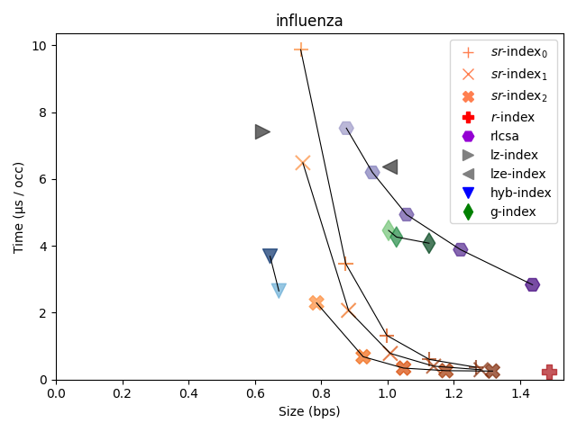
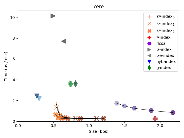
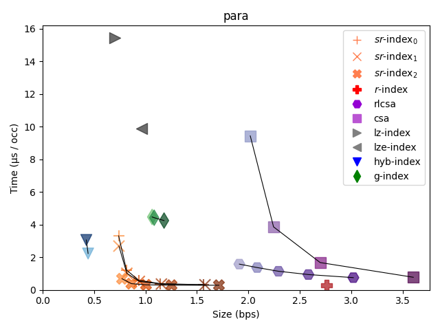
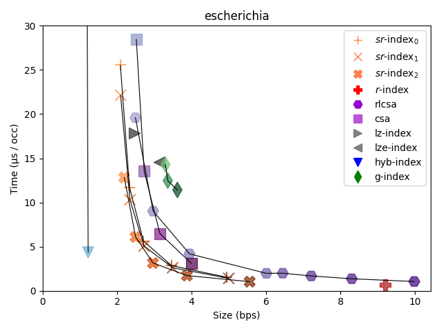
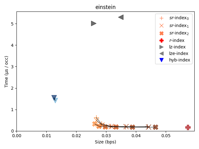
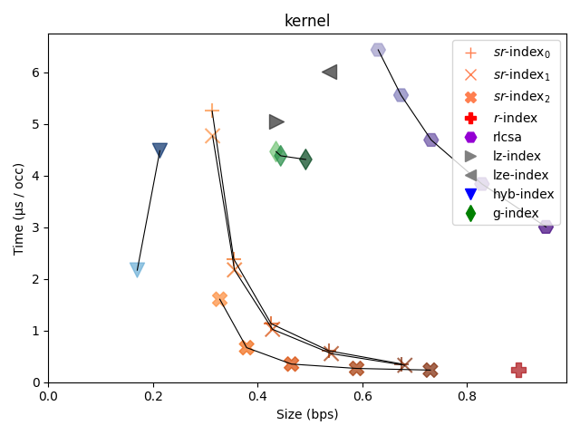
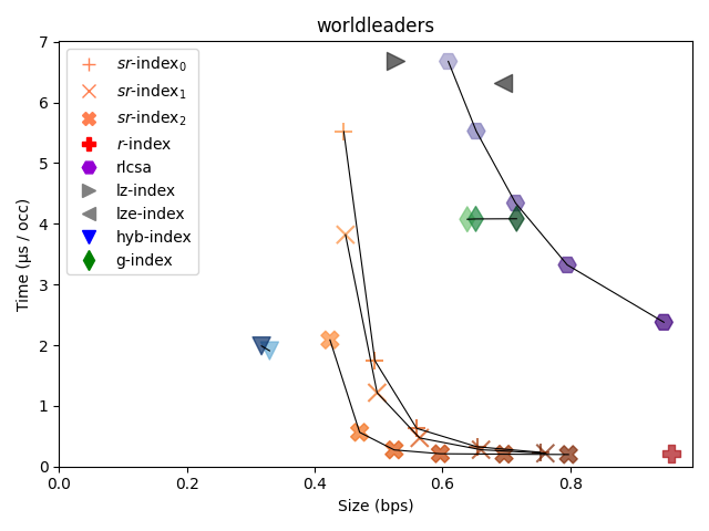
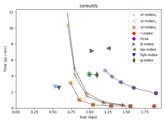
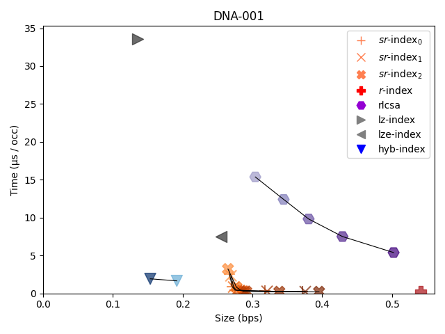
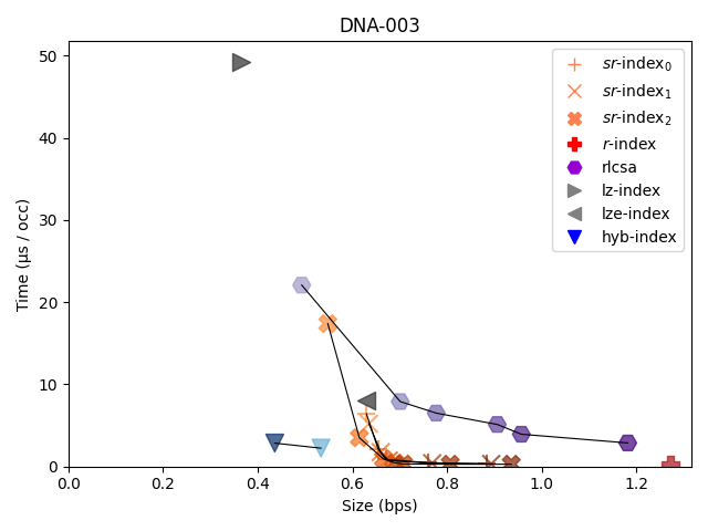
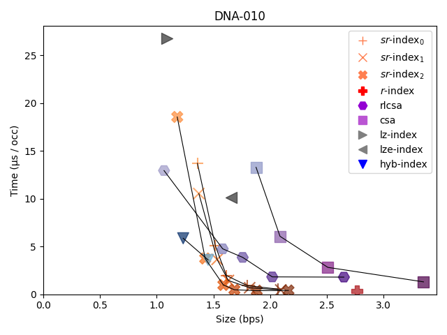
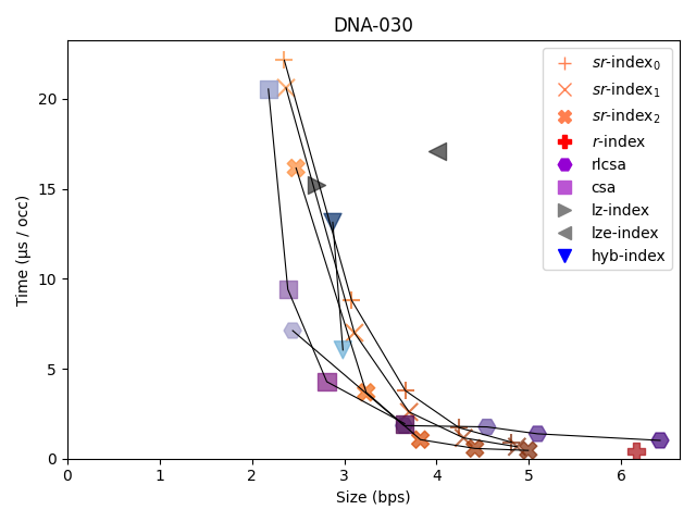
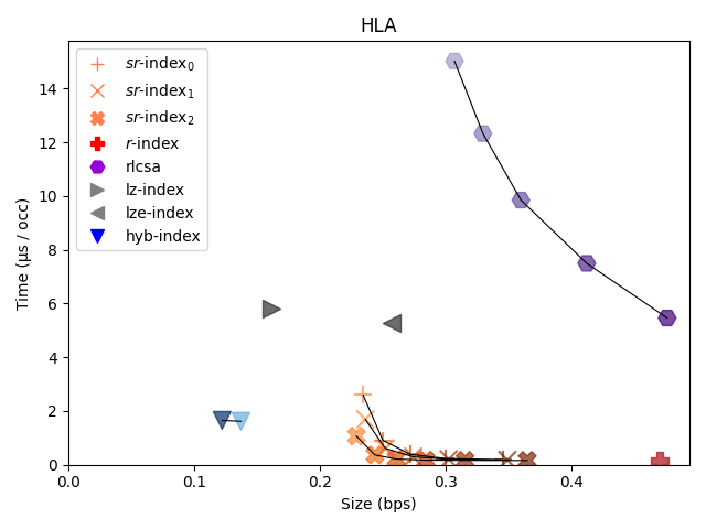
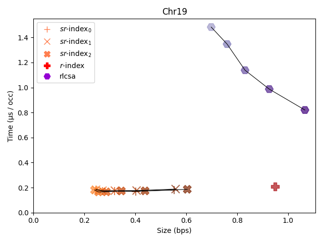
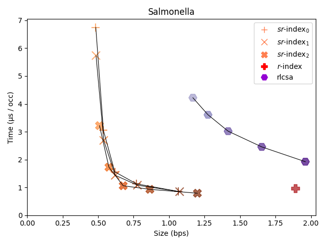
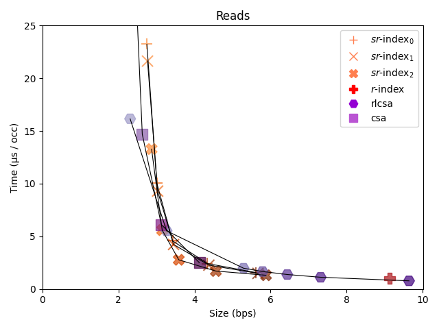
A first conclusion is that always dominates and , so we will refer to it simply as sr-index from now on. The plots show that the extra information we associate to the samples makes a modest difference in space, while time improves considerably. This sr-index can be almost as fast as the r-index, and an order of magnitude faster than all the others, while using – less space than the r-index. Therefore, as promised, we are able to remove a significant degree of redundancy in the r-index without affecting its outstanding time performance.
In all the PizzaChili collections, the sr-index dominates almost every other index, outperforming them both in time and space. The only other index on the Pareto curve is the hyb-index, which can use as little as a half of the space of the sweet spot of the sr-index, but still at the price of being an order of magnitude slower. This holds even on escherichia, where is well below , and both the rlcsa and the csa become closer to the sr-index.
In general, in all the collections with sufficient repetitiveness, say over 25, the sr-index sharply dominates as described. As repetitiveness decreases, with reaching around 10, the rlcsa and the csa approach the sr-index and outperform every other repetitiveness-aware index, as expected. This happens on escherichia (as mentioned) and Reads (where the sr-index, the rlcsa, and the csa behave similarly). This is also the case on the least repetitive synthetic DNA collection, DNA-030, where the mutation rate reaches 3%. In this collection, the repetitiveness-unaware csa largely dominates all the space-time map.
We expected the sr-index to have a bigger advantage over the r-index on the HLA dataset because its oversampling is concentrated, but the results are similar to those on randomly mutated DNA with about the same value (DNA-001). In general, the bps used by the sr-index can be roughly predicted from ; for example the sweet spot often uses around total bits, although it takes – bits in some cases. The r-index uses – bits.
The bigger collections (Chr19, Salmonella, Reads), on which we could build the -related indexes only, show that the same observed trends scale to gigabyte-sized collections of various repetitiveness levels.
6 Conclusions
We have introduced the sr-index, an r-index variant that solves the problem of its relatively bloated space while retaining its high search performance. The sr-index is orders of magnitude faster than the other repetitiveness-aware indexes, while outperforming most of them in space as well. It matches the time performance of the r-index while using – less space.
Unlike the r-index, the sr-index uses little space even in milder repetitiveness scenarios, which makes it usable in a wider range of bioinformatic applications. For example, it uses 0.25–0.60 bits per symbol (bps) while reporting each occurrence within a microsecond on gigabyte-sized human and bacterial genomes, where the original r-index uses 0.95–1.90 bps. In general, the sr-index outperforms classic compressed indexes on collections with repetitiveness levels over as little as in some cases, though in general it is reached by repetitiveness-unaware indexes when approaches , which is equivalent to a DNA mutation rate around 3%.
Compared to the rlfm-index, which for pattern searching is dominated by the sr-index, the former can use its regular text sampling to compute any entry of the suffix array or its inverse in time proportional to the sampling step . Obtaining an analogous result on the sr-index, for example to implement compressed suffix trees, is still a challenge. Other proposals for accessing the suffix array faster than the rlfm-index [12, 26] illustrate this difficulty: they require even more space than the r-index.
References
- [1] Christina Boucher, Ondrej Cvacho, Travis Gagie, Jan Holub, Giovanni Manzini, Gonzalo Navarro, and Massimiliano Rossi. PFP compressed suffix trees. In Proc. 23rd Workshop on Algorithm Engineering and Experiments (ALENEX), pages 60–72, 2021.
- [2] Christina Boucher, Travis Gagie, Alan Kuhnle, Ben Langmead, Giovanni Manzini, and Taher Mun. Prefix-free parsing for building big BWTs. Algorithms for Molecular Biology, 14(1):13:1–13:15, 2019.
- [3] Michael Burrows and David J. Wheeler. A block-sorting lossless data compression algorithm. Technical Report 124, Digital Equipment Corporation, 1994.
- [4] D. R. Clark. Compact PAT Trees. PhD thesis, University of Waterloo, Canada, 1996.
- [5] Francisco Claude, Gonzalo Navarro, and Alejandro Pacheco. Grammar-compressed indexes with logarithmic search time. Journal of Computer and System Sciences, 118:53–74, 2021.
- [6] Diego Díaz-Domínguez and Gonzalo Navarro. A grammar compressor for collections of reads with applications to the construction of the BWT. In Proc. 31st Data Compression Conference (DCC), 2021. To appear.
- [7] Héctor Ferrada, Dominik Kempa, and Simon J. Puglisi. Hybrid indexing revisited. In Proc. 20th Workshop on Algorithm Engineering and Experiments (ALENEX), pages 1–8, 2018.
- [8] Paolo Ferragina and Giovanni Manzini. Indexing Compressed Text. Journal of the ACM, 52(4):552–581, 2005.
- [9] Paolo Ferragina, Giovanni Manzini, Veli Mäkinen, and Gonzalo Navarro. Compressed Representations of Sequences and Full-text Indexes. ACM Transactions on Algorithms, 3(2), 2007.
- [10] T. Gagie and G. Navarro. Compressed Indexes for Repetitive Textual Datasets. Springer, 2019.
- [11] Travis Gagie, Gonzalo Navarro, and Nicola Prezza. Fully-functional suffix trees and optimal text searching in BWT-runs bounded space. Journal of the ACM, 67(1):article 2, 2020.
- [12] Rodrigo González, Gonzalo Navarro, and Héctor Ferrada. Locally compressed suffix arrays. ACM Journal of Experimental Algorithmics, 19(1):article 1, 2014.
- [13] Dominik Kempa and Tomasz Kociumaka. Resolution of the Burrows-Wheeler transform conjecture, 2019. To appear in FOCS 2020. arXiv:1910.10631.
- [14] John C. Kieffer and En-Hui Yang. Grammar-based codes: A new class of universal lossless source codes. IEEE Transactions on Information Theory, 46(3):737–754, 2000.
- [15] Sebastian Kreft and Gonzalo Navarro. On compressing and indexing repetitive sequences. Theoretical Computer Science, 483:115–133, 2013.
- [16] Abraham Lempel and Jacob Ziv. On the complexity of finite sequences. IEEE Transactions on Information Theory, 22(1):75–81, 1976.
- [17] Veli Mäkinen, Djamal Belazzougui, Fabio Cunial, and Alexandru I. Tomescu. Genome-Scale Algorithm Design. Cambridge University Press, 2015.
- [18] Veli Mäkinen and Gonzalo Navarro. Succinct suffix arrays based on run-length encoding. Nordic Journal of Computing, 12(1):40–66, 2005.
- [19] Veli Mäkinen, Gonzalo Navarro, Jouni Sirén, and Niko Välimäki. Storage and retrieval of highly repetitive sequence collections. Journal of Computational Biology, 17(3):281–308, 2010.
- [20] Udi Manber and Gene Myers. Suffix arrays: a new method for on-line string searches. SIAM Journal on Computing, 22(5):935–948, 1993.
- [21] Gonzalo Navarro. Indexing highly repetitive string collections. CoRR, 2004.02781, 2020. To appear in ACM Computing Surveys.
- [22] Gonzalo Navarro and Veli Mäkinen. Compressed full-text indexes. ACM Computing Surveys, 39(1):article 2, 2007.
- [23] Gonzalo Navarro and Víctor Sepúlveda. Practical indexing of repetitive collections using Relative Lempel-Ziv. In Proc. 29th Data Compression Conference (DCC), pages 201–210, 2019.
- [24] Takaaki Nishimoto and Yasuo Tabei. Faster queries on BWT-runs compressed indexes. CoRR, 2006.05104, 2020.
- [25] Daisuke Okanohara and Kunihiko Sadakane. Practical entropy-compressed rank/select dictionary. In Proc. 9th Workshop on Algorithm Engineering and Experiments (ALENEX), pages 60–70, 2007.
- [26] Simon J. Puglisi and Bella Zhukova. Relative Lempel-Ziv compression of suffix arrays. In Proc. 27th International Symposium on String Processing and Information Retrieval (SPIRE), pages 89–96, 2020.
- [27] James Robinson, Dominic J. Barker, Xenia Georgiou, Michael A. Cooper, Paul Flicek, and Steven G. E. Marsh. IPD-IMGT/HLA Database. Nucleic Acids Research, 48(D1):D948–D955, 10 2019. doi:10.1093/nar/gkz950.
- [28] Kunihiko Sadakane. New text indexing functionalities of the compressed suffix arrays. Journal of Algorithms, 48(2):294–313, 2003.
- [29] Eric L. Stevens, Ruth Timme, Eric W. Brown, Marc W. Allard, Errol Strain, Kelly Bunning, and Steven Musser. The public health impact of a publically available, environmental database of microbial genomes. Frontiers in Microbiology, 8:808, 2017.
- [30] The 1000 Genomes Project Consortium. A global reference for human genetic variation. Nature, 526:68–74, 2015.