Fooling LiDAR Perception via Adversarial Trajectory Perturbation

Abstract

LiDAR point clouds collected from a moving vehicle are functions of its trajectories, because the sensor motion needs to be compensated to avoid distortions. When autonomous vehicles are sending LiDAR point clouds to deep networks for perception and planning, could the motion compensation consequently become a wide-open backdoor in those networks, due to both the adversarial vulnerability of deep learning and GPS-based vehicle trajectory estimation that is susceptible to wireless spoofing? We demonstrate such possibilities for the first time: instead of directly attacking point cloud coordinates which requires tampering with the raw LiDAR readings, only adversarial spoofing of a self-driving car’s trajectory with small perturbations is enough to make safety-critical objects undetectable or detected with incorrect positions. Moreover, polynomial trajectory perturbation is developed to achieve a temporally-smooth and highly-imperceptible attack. Extensive experiments on 3D object detection have shown that such attacks not only lower the performance of the state-of-the-art detectors effectively, but also transfer to other detectors, raising a red flag for the community. The code is available on https://ai4ce.github.io/FLAT/.

1 Introduction

Autonomous driving systems are generally equipped with all kinds of sensors to perceive the complex environment [7]. Among the sensors, LiDAR has played a crucial role due to its plentiful geometric information sampled by incessantly spinning a set of laser emitters and receivers. However, LiDAR scans are easily distorted by vehicle’s motion, , the points in a full sweep are sampled at different timestamps when vehicle is at different locations and orientations, as shown in Fig. 1. Imagine that a self-driving car is on a highway at a speed of 30m/s, its LiDAR with a 20Hz scanning frequency would move 1.5 meters during a full sweep, severely distorting the captured point cloud.

Figure 1: Illustration of our trajectory-based attack and the motion correction process. The top right and bottom right figures are respectively original and distorted LiDAR sweep as well as the detection results. Green/red boxes denote the ground truth/prediction. In this example, our method (named as FLAT) makes the detector miss eight out of eleven vehicles.

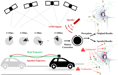
Such distortions are typically compensated by querying the vehicle/LiDAR’s pose at any time from a continuous vehicle ego-motion tracking module that fuses pose estimation from Global Navigation Satellite System (GNSS, , GPS, GLONASS, and BeiDou), Inertial Navigation System (INS), and SLAM-based localization using LiDAR or cameras. Well-known LiDAR datasets like KITTI [7] and nuScenes [2] have already corrected such motion distortions prior to the dataset release. Researchers then made impressive progresses by processing those distortion-free point clouds using deep neural networks (DNNs) for many tasks, , 3D object detection, semantic/instance segmentation, motion prediction, multiple object tracking.

However, using DNNs on LiDAR point clouds creates a potentially dangerous and less cognizant vulnerability in self-driving systems. First, the above perception tasks are functions of LiDAR point clouds implemented via DNNs. Second, the motion compensation makes LiDAR point clouds a function of the vehicle trajectories. This functional composition leads to a simple but surprising fact that those perception tasks are now also functions of the trajectories. Thus, such a connection exposes the well-known adversarial robustness issue of DNNs to hackers who could now fool a self-driving car’s safety-critical LiDAR-depending perception modules by calculatedly spoofing the area’s wireless GNSS signals, which is still a serious and unresolved security problem demonstrated on many practical systems [30, 23, 52]. Luckily, given that the aforementioned non-GNSS pose sources such as INS and visual SLAM are fused together for vehicle ego-motion estimation, large variations (meter-level) of GNSS trajectory spoofing could be detected and filtered, ensuring a safe localization and mapping for self-driving cars. However, what if a spoofed trajectory only has dozens of centimeters offset? Would current point cloud DNNs be robust enough under such small variations?

In this paper, we initiate the first work to reveal and investigate such a vulnerability. Different from existing works directly attacking point cloud coordinates with 3D point perturbations or adversarial object generation [41, 36, 44, 9], we propose to fool LiDAR-based perception modules by attacking the vehicle trajectory, which could be detrimental and easily deployable in the physical world. Our investigation includes how to obtain LiDAR sweeps with simulated motion distortion from real-world datasets, convert LiDAR point clouds as a differentiable function of the vehicle trajectories, and eventually calculate the adversarial trajectory perturbation and make them less perceptible. Our principal contributions are as follows:

• We propose an effective approach for simulating motion distortion using a sequence of real-world LiDAR sweeps from existing dataset.

• We propose a novel view of LiDAR point clouds as a differentiable function of the vehicle trajectories, based on the real-world motion compensation process.

• We propose to Fool LiDAR perception with Adversarial Trajectory (FLAT), which has better feasibility and transferability (code will be released).

• We conduct extensive experiments on 3D object detection as a downstream task example, and show that the advanced detectors can be effectively blinded.

2 Related Work

GNSS/INS and LiDAR Motion Compensation. Motion distortion is also known as motion blur or rolling shutter effect of LiDAR on ego-motion vehicles [20]. To compensate for such distortions, GNSS/INS is often used to provide the pose of the LiDAR at any moment when a point is scanned. This opens backdoors for a self-driving system. First, space weather is a substantial error source for GNSS and also significantly affects systems such as differential GPS. The influence of ionosphere disturbances on GPS kinematic precise point positioning (PPP) can be larger than 2 to 10 meters at different latitudes [49], while solar radio burst could cause GPS positioning errors as large as 300 meters vertically and 50 meters horizontally [22]. Besides those naturally occurring events, malicious attacks such as GPS jamming or spoofing could also be used to arbitrarily modify the GPS trajectory [30, 23, 52]. Moreover, when GNSS and INS are fused, such attacks can affect not only positions but also the rotational component (gyroscope bias compensation) of a vehicle’s trajectory [46]. Of course, nowadays for motion compensation, LiDAR poses are usually fused between GNSS/INS and LiDAR-/camera-based localization, so large pose variations from extreme space weather or “urban canyon” effect could be filtered. But as long as GNSS is a part of the equation, the backdoors could remain open, especially when the spoofed trajectories only have small variations from the ground truth, as we show later.

Image-based Adversarial Attack. Despite the great success achieved by deep learning in both academia and industry, researchers have found that deep networks are susceptible to carefully-designed adversarial perturbation which is hard to distinguish. Since such vulnerability is firstly pointed out in image classification task [35], broad attentions have been paid to adversarial robustness in various downstream tasks, , semantic segmentation [45], object detection [24], visual tracking [8], . Adversarial attack is divided into white box [21] and black box [1] based on whether the model parameters are known. Besides, attacks can be categorized as targeted [47] and untargeted [42] according to whether the adversary has a particular goal. Meanwhile, many attempts have been made in defense mechanisms, such as adversarial training [19], certified defense [28, 51], adversarial example detector [51], and ensemble diversity [25]. Extensive studies in image-based adversarial attack and defense have largely promoted the development of trustworthy machine learning in 2D computer vision and inspired similar investigations in 3D vision.

Point Cloud Attack and Defense. Recently, researchers have explored the vulnerability of DNNs taking point clouds of 3D objects as input. For the object-level point cloud attack, Xiang et al. [44] proposed point perturbation as well as cluster generation to attack the widely-used PointNet [26]. Besides, critical points removal [41, 48], adversarial deformation [54], geometric-level attack [15] are proposed for fooling the point cloud-based deep model. However, none of them directly target LiDAR point clouds of self-driving scenes which have domain gaps than object-level point clouds. Moreover, to implement the above point cloud attacks towards a self-driving car requires tampering with its software for altering point cloud coordinates. Differently, our paper reveals a simple yet dangerous possibility of spoofing the trajectory to attack deep modules through the LiDAR motion correction process yet without any need of software hacking. As for the works on scene-level point cloud attack, Tu et al. [36] proposed to generate 3D adversarial shapes placed on the rooftop of a target vehicle, making the target invisible for the detectors. Some works [3, 34, 32, 4] created spoofing obstacles/faked points in front of the car to influence the vehicle’s decision, but they can only modify the limited area of the scene. Differently, our method does not need to physically alter any shapes in the scene, and can easily scale up the attack to the whole scene. In a word, existing works directly manipulate on the point coordinates either physically or virtually, while our attack is realized by spoofing the vehicle trajectories.

Affected Downstream Tasks. Theoretically, every downstream task that require LiDAR point cloud as input could be affected by the attacks proposed in this paper. This could include geometric vision tasks such as registration, pose estimation, and mapping, as well as pattern recognition tasks such as 3D object detection [14, 50, 31, 55, 16, 38], semantic segmentation [13, 12], motion prediction [43, 17, 53], and multiple object tracking [39, 40]. While the first group of tasks could be less severely affected by GNSS spoofing via data fusion as mentioned above, the second group has higher vulnerability, because small but calculated perturbations in the point coordinates could affect deep networks as demonstrated in the above related works. In this paper, without loss of generality, we choose to focus on the 3D object detection task to illustrate the severity of this backdoor, because miss detection of safety-critical objects surrounding a self-driving car could be a matter of life or death.

3 Motion Distortion in LiDAR

LiDAR measurements are obtained along with the rotation of its beams, so the measurements in a full sweep are captured at different timestamps, introducing motion distortion which jeopardizes the vehicle perception. Autonomous systems generally utilize LiDAR’s location and orientation obtained from the localization system to correct distortion [29, 6, 10]. Most LiDAR-based datasets [2, 7] have finished synchronization before release. Hence, the performance of current 3D perception algorithms in the distorted point cloud remains unexplored. We briefly introduce the nomenclature in this work before detailed illustrations.

World Frame. We use a coordinate frame $W$ fixed in the world with the orthonormal basis $\{\mathbf{x}_{W},\mathbf{y}_{W},\mathbf{z}_{W}\}$ to describe the global displacement of the self-driving car.

Object Frame. The car can be associated with a right-handed, orthonormal coordinate frame which can describe its rigid body motion. Such a frame attached to the car is called object frame [18]. In the following, we use frame to denote the object frame of the car at different timestamps.

Sweep&Packet. LiDAR points in a complete 360^∘ is called a sweep, and the points are emitted as a stream of packets, each covering a sector of the 360^∘ coverage [10].

3.1 Linear Pose Interpolation

Figure 2: Diagram of motion distortion simulation. Firstly, we interpolate $N$ steps in 6DoF pose between two adjacent frames $A$ and $B$. Secondly, we divide a sweep at frame $A$ into $N$ packets, and the $n$-th sector corresponds to the $n$-th interpolated frame. Thirdly, we transform the point cloud in the $n$-th packet at frame $A$ into frame $n$ with homogeneous transformation ${\mathbf{T}^{n}_{A}}$. Finally, motion-distorted point cloud can be generated by aggregating the point cloud from frame $0$ to frame $N-1$.

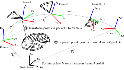
In this section, we recover the raw point cloud before synchronization with a sequence of real-world LiDAR point clouds from nuScenes [2]. Each sample of nuScenes provides a sweep and its corresponding ego pose. We assume the vehicle is moving smoothly and carry out linear pose interpolation between two adjacent frames $A$ and $B$, as shown in Fig. 2. $\{\mathbf{x}_{A},\mathbf{y}_{A},\mathbf{z}_{A}\}$ and $\{\mathbf{x}_{B},\mathbf{y}_{B},\mathbf{z}_{B}\}$ are their orthonormal basis. Using $\mathbf{t}_{A}\in\mathbb{R}^{3}$ and $\mathbf{t}_{B}\in\mathbb{R}^{3}$ to represent global translation of frame $A$ and $B$, the global translation of the $n$-th ($n=0,1,2,...,N-1$) interpolated frame is:

$$\mathbf{t}(n)=\mathbf{t}_{A}+\frac{\mathbf{t}_{B}-\mathbf{t}_{A}}{N}\times n\ ,$$ (1)

where $N$ is the total interpolation steps. For the orientation, we implement spherical linear interpolation (slerp) [33]. Using $\mathbf{q}_{A}=\left[q^{A}_{w},q^{A}_{x},q^{A}_{y},q^{A}_{z}\right]^{\top}$ and $\mathbf{q}_{B}=\left[q^{B}_{w},q^{B}_{x},q^{B}_{y},q^{B}_{z}\right]^{\top}$ to represent quaternion at frame $A$ and $B$, then the quaternion at the $n$-th interpolated frame is:

$$\mathbf{q}(n)=\frac{\sin((1-n)\theta)}{\sin\theta}\mathbf{q}_{A}+\frac{\sin(n\theta)}{\sin\theta}\mathbf{q}_{B}\ ,$$ (2)

where $\theta=\cos^{-1}\left(\mathbf{q}_{A}\cdot\mathbf{q}_{B}\right)$ is the rotation angle between $A$ and $B$. Convert the quaternion $\mathbf{q}(n)=\left[q^{n}_{w},q^{n}_{x},q^{n}_{y},q^{n}_{z}\right]^{\top}$ to the rotation matrix $\mathbf{R}(n)\in SO(3)$, then

the homogeneous transformation matrix from the world frame $W$ to the $n$-th interpolated frame denoted as $\mathbf{T}^{W}_{n}\in SE(3)$ is:

$$\mathbf{T}^{W}_{n}=\left[\begin{array}[]{cc}\mathbf{R}(n)&\mathbf{t}(n)\\ \mathbf{0}_{1\times 3}&1\end{array}\right]\ .$$ (3)

3.2 Motion Distortion Simulation

After linear pose interpolation, we can get $N$ more frames. To simulate motion distortion, we assume that the sweep at frame $A$ is aggregated from $N$ frames, and in each frame, the beam scans a degree of $\frac{360}{N}$. Therefore, we firstly divide the sweep at frame $A$ into $N$ packets, as shown in Fig. 2. Then we transform the LiDAR packet $n$ to the coordinate of frame $n$ at which the point cloud is assumed to be captured. The points in packet $n$ at frame $A$ (denoted as $\prescript{A}{}{\mathbf{P}_{n}}\in\mathbb{R}^{4\times m_{n}}$) is represented as a set of 3D points $\{P_{m}|m=1,2,...,m_{n}\}$, where each point $P_{m}$ is a vector of its homogeneous coordinate $(x,y,z,1)$, and $m_{n}$ denotes the number of points in packet $n$. We transform $\prescript{A}{}{\mathbf{P}_{n}}$ to its corresponding capture frame $n$:

$$\prescript{n}{}{\mathbf{P}}={\mathbf{T}^{n}_{A}}\prescript{A}{}{\mathbf{P}_{n}}\ ,$$ (4)

where $\prescript{n}{}{\mathbf{P}}\in\mathbb{R}^{4\times m_{n}}$ is the point cloud of packet $n$ in the coordinate of frame $n$ (can be treated as the point cloud captured at frame $n$) and ${\mathbf{T}^{n}_{A}}$ is the homogeneous transformation from frame $n$ to frame $A$ and is as follows:

$${\mathbf{T}^{n}_{A}}={\mathbf{T}^{n}_{W}}{\mathbf{T}^{W}_{A}}=({\mathbf{T}^{W}_{n}})^{-1}{\mathbf{T}^{W}_{A}}\ ,$$ (5)

where ${\mathbf{T}^{W}_{n}}$ is from Eq. (3) and ${\mathbf{T}^{W}_{A}}$ can also be calculated given $\mathbf{t}_{A}$ and $\mathbf{q}_{A}$. Finally, a set of motion-distorted point clouds ${}^{A}\widetilde{\mathbf{P}}\in\mathbb{R}^{4\times m}$ is generated by aggregating multiple LiDAR packets captured at different frames:

$$^{A}\widetilde{\mathbf{P}}=[\prescript{0}{}{\mathbf{P}};\prescript{1}{}{\mathbf{P}};...;\prescript{N-1}{}{\mathbf{P}}]\ ,$$ (6)

where $[\cdot;\cdot;...;\cdot]$ is the concatenation operation along the row. It is noted that $m=\sum_{n=0}^{N-1}m_{n}$.

3.3 Motion Compensation with Ego-Pose

Up to now, we have generated motion-distorted point cloud as shown in Eq. 6, and then we can represent the motion compensation using the mathematical formula, , a LiDAR sweep can be written as a differentiable function of the vehicle trajectory. The undistorted point cloud ${{}^{A}\mathbf{P}}\in\mathbb{R}^{4\times m}$ is obtained by transforming point clouds from frame $0\thicksim N-1$ back to the coordinate of frame $A$:

$${\prescript{A}{}{\mathbf{P}}}=[{\mathbf{T}^{A}_{0}}\prescript{0}{}{\mathbf{P}};{\mathbf{T}^{A}_{1}}\prescript{1}{}{\mathbf{P}};...;{\mathbf{T}^{A}_{N-1}}\prescript{N-1}{}{\mathbf{P}}]\ ,$$ (7)

where ${\mathbf{T}^{A}_{n}}$ is the transformation from frame $A$ to frame $n$, which is the inverse matrix of ${\mathbf{T}^{n}_{A}}$ in Eq. (5).

4 Adversarial Trajectory Perturbation

4.1 Point Cloud Representation w.r.t. Trajectory

The studies of object-level point cloud generally treat point cloud as a set of 3D points sampled from mesh models instantaneously [44, 9]. In autonomous driving, however, the 3D points are captured in a dynamic setting through raycasting, thus LiDAR not only records points’ $(x,y,z)$ coordinates, but also the timestamps at which the points are captured. To this end, we propose a novel representation of point cloud as a function of vehicle trajectory through Eq. (7) which can be written as a general form:

$${\mathbf{P}}={f}(\mathbf{T},L(\prescript{n}{}{\mathbf{P}})),\ \ n=0,1,...,N-1\ ,$$ (8)

where ${\mathbf{P}}\in\mathbb{R}^{4\times m}$ is a full sweep with $m$ points, and is represented as a differentiable function $f$ in terms of vehicle trajectory $\mathbf{T}\in\mathbb{R}^{N\times 4\times 4}$ and the list of LiDAR packets $L(\prescript{n}{}{\mathbf{P}})=[\prescript{0}{}{\mathbf{P}},\prescript{1}{}{\mathbf{P}},...,\prescript{N-1}{}{\mathbf{P}}]$ ($\prescript{n}{}{\mathbf{P}}\in\mathbb{R}^{4\times m_{n}}$). Noted that the trajectory between two adjacent frames is represented as a set of homogeneous transformation matrices. Different from previous works tampering with point coordinates [44], we propose to represent point cloud as a function of trajectory, and attack the trajectory instead of 3D points. Our method has the following advantages.

Physical Feasibility. Since the motion compensation is naturally occurring in self-driving, it is physically-realizable and straightforward to attack the trajectory, , by wireless GNSS spoofing. In contrast, coordinate attack requires software hacking which is infeasible in practice.

Better Transferability. Our learned trajectory perturbation with the same size ($N\times 4\times 4$) can be easily transferred to different sweeps. Yet, coordinate attacks cannot be transferred across sweeps because different sweeps could have different numbers of points, and the perturbation in the point space could have different dimensions.

Novel Parameterization. We attack the 6-DoF pose of each packet, but coordinate attack modifies a single point’s xyz position without orientations. Hence, our method has better performance due to new attacked parameters.

4.2 Objective Function

Since the point cloud is represented as a differentiable function of the trajectory, the gradient can be back-propagated to the trajectory smoothly for adversarial learning. The adversarial objective is to minimize the negative loss function of the deep model with parameter $\theta$:

$$\min\widetilde{\mathcal{L}}(\theta,{f}(\mathbf{T},L(\prescript{n}{}{\mathbf{P}})),\mathbf{y})\ ,$$ (9)

where $\mathbf{y}$ is the desired output of the network, ${f}(\mathbf{T},L(\prescript{n}{}{\mathbf{P}}))$ is the input point cloud as a function of the trajectory. Assume that we are assigned to attack a downstream task with loss function ${\mathcal{L}}$, , cross-entropy loss in classification, then $\widetilde{\mathcal{L}}=-{\mathcal{L}}$. Afterwards, the adversarial perturbation $\bm{\delta}\in\mathbb{R}^{N\times 4\times 4}$ can be obtained via projected gradient descent (PGD) with multiple iterations [19]:

$$\small\bm{\delta}^{t+1}=\mathcal{P}\left(\bm{\delta}^{t}-\alpha\operatorname{sgn}\left(\nabla_{\bm{\delta}}\widetilde{\mathcal{L}}(\theta,{f}(\mathbf{T}+\bm{\delta},L(\prescript{n}{}{\mathbf{P}})),\mathbf{y})\right)\right)\ ,$$ (10)

where $t$ denotes iteration number, $\mathcal{P}$ indicates the projection onto the convex set of interest, and this work uses clipping which is the case of $\ell_{\infty}$ norm to ensure an acceptable perturbation magnitude. The $n$-th element in $\bm{\delta}$ in the matrix form is:

$$\bm{\delta}(n)=\left[\begin{array}[]{cc}\widetilde{\mathbf{R}}(n)&\widetilde{\mathbf{t}}(n)\\ \mathbf{0}_{1\times 3}&1\end{array}\right]\ .$$ (11)

Polynomial Trajectory Perturbation. To make the attack highly imperceptible, the polynomial trajectory perturbation is proposed: we define the perturbation in translations as a third-order polynomial of time as follows:

$$\small\widetilde{\mathbf{t}}(n)={\bm{\beta}}^{T}\mathbf{n}\ ,$$ (12)

where $\mathbf{n}=[1,n,n^{2},n^{3}]^{\top}$ and $\bm{\beta}=[\bm{\beta_{x}},\bm{\beta_{y}},\bm{\beta_{z}}]$ is the polynomial coefficients. Now $\bm{\delta}$ is a differentiable function of $\bm{\beta}$, and the gradient will be back-propagated to $\bm{\beta}$, so the adversarial coefficients are calculated by:

$$\small\bm{\beta}^{t+1}=\mathcal{P}\left(\bm{\beta}^{t}-\alpha\operatorname{sgn}\left(\nabla_{\bm{\beta}}\widetilde{\mathcal{L}}(\theta,{f}(\mathbf{T}+\bm{\delta},L(\prescript{n}{}{\mathbf{P}})),\mathbf{y})\right)\right)\ ,$$ (13)

hence, we only need to manipulate several key points to bend a polynomial-parameterized trajectory which can be easily achieved in reality, achieving a real-time attack.

4.3 Attack with Regularization

Regularization on Trajectory. To realize an imperceptible attack, we propose a trajectory smoothness regularizer to repress the total variation in vehicle poses. Given a trajectory perturbation $\bm{\delta}\in\mathbb{R}^{N\times 4\times 4}$, we calculate the difference in translation and rotation separately. The smoothness $\mathcal{S}(\bm{\delta})$ equals to the following formula:

$$\small\lambda_{\mathbf{t}}(\sum^{N-1}_{n=1}(\widetilde{\mathbf{t}}(n)-\widetilde{\mathbf{t}}(n-1))^{p})^{\frac{1}{p}}+\lambda_{\mathbf{R}}(\sum^{N-1}_{n=1}(\widetilde{\mathbf{R}}(n)-\widetilde{\mathbf{R}}(n-1))^{p})^{\frac{1}{p}}\ ,$$ (14)

where $\lambda_{\mathbf{t}}$ and $\lambda_{\mathbf{R}}$ are used to balance the influence of translations and rotations, $p$ denotes the norm ($p=2$ in this work). With trajectory smoothness regularization, the objective of adversarial attacks is as follows:

$$\min\widetilde{\mathcal{L}}(\theta,{f}(\mathbf{T}+\bm{\delta},L(\prescript{n}{}{\mathbf{P}})),\mathbf{y})+\lambda_{s}\mathcal{S}(\bm{\delta})\ ,$$ (15)

where $\lambda_{s}$ is for adjusting the smoothness degree. By optimizing over Eq. (15), we aim to find an imperceptible adversarial perturbation $\bm{\delta}$ with desirable smoothness.

Regularization on Point Cloud. We also propose a regularizer on point cloud to repress its change. We use two metrics to measure the variation of point cloud before and after distortion, , $\ell_{p}$ norm and Chamfer distance [5]. Using $\mathcal{D}_{L}(\bm{\delta})$ to denote $\ell_{p}$ distance, $\mathcal{D}_{C}(\bm{\delta})$ to denote Chamfer distance before and after perturbation $\bm{\delta}$. The adversarial objective with regularization is defined as:

$$\min\widetilde{\mathcal{L}}(\theta,{f}(\mathbf{T}+\bm{\delta},L(\prescript{n}{}{\mathbf{P}})),\mathbf{y})+\lambda_{d}\mathcal{D}(\bm{\delta})\ ,$$ (16)

where $\mathcal{D}(\bm{\delta})$ can be either $\mathcal{D}_{L}(\bm{\delta})$ or $\mathcal{D}_{C}(\bm{\delta})$. $\lambda_{d}$ is to control the degree of distortion. By optimizing over Eq. (16), we try to search for a powerful adversarial perturbation $\bm{\delta}$ leading to subtle distortion in the point cloud.

Table 1: Quantitative results of white box attack: AP (IoU=0.7) of 3D bounding boxes on nuScenes [2]. We report results of the car category under different levels of difficulty and ranges of depth following [37]. In four attack settings of our method (FLAT), the best and second best attack qualities among four attacking targets are respectively highlighted using red and blue color. In attacking translations/rotations, the step size for each iteration is 0.1 and 0.01 respectively, and the number of attack iteration is 20 for both two settings.

Attack Approach  $\backslash$  Case			Easy	Moderate	Hard	0-30m	30-50m	50-70m
PointRCNN [31]			47.44	21.56	20.91	47.44	2.16	0.17
Baseline	Coordinate Attack [44]		16.42	6.58	5.90	15.20	0.48	0.03
	Random Attack (Point Cloud)		30.09	12.39	10.84	25.65	0.79	0.06
	Random Attack (Translation)		17.00	8.58	8.90	20.43	1.09	0.09
	Random Attack (Rotation)		12.30	4.87	5.13	13.31	0.01	0.00
	Random Attack (Full Trajectory)		5.66	2.43	2.78	7.67	0.02	0.00
FLAT (Translation)	Classification	Stage-1	12.94	6.58	7.22	16.82	0.86	0.06
		Stage-2	11.72	5.87	6.06	13.91	0.87	0.04
	Regression	Stage-1	17.46	8.24	8.57	19.36	1.09	0.03
		Stage-2	26.09	12.78	12.53	27.15	2.17	0.17
FLAT (Polynomial)	Classification	Stage-1	17.94	9.36	9.56	20.73	1.90	0.19
		Stage-2	12.51	6.37	6.54	14.51	1.38	0.16
	Regression	Stage-1	22.60	11.01	10.96	24.36	1.67	0.15
		Stage-2	26.04	12.76	12.51	27.19	2.17	0.17
FLAT (Rotation)	Classification	Stage-1	6.32	2.43	2.51	7.32	0.02	0.00
		Stage-2	2.35	0.80	0.61	2.03	0.01	0.00
	Regression	Stage-1	5.50	1.87	1.76	5.45	0.02	0.00
		Stage-2	26.30	12.89	12.59	27.35	2.17	0.17
FLAT (Full Trajectory)	Classification	Stage-1	1.52	0.45	0.51	1.71	0.01	0.00
		Stage-2	0.19	0.01	0.02	0.26	0.00	0.00
	Regression	Stage-1	1.01	0.35	0.32	1.27	0.01	0.00
		Stage-2	26.03	12.70	12.48	27.13	2.16	0.17

5 Experiments

5.1 Target 3D Deep Model

In this work, we select widely-studied LiDAR-based 3D detection, which aims to estimate 3D bounding boxes of the objects in point cloud, as a downstream task example to verify our attack pipeline. Currently, LiDAR-based detection has two mainstreams: 1) point-based method directly consuming raw point cloud data, 2) voxel-based method which requires non-differentiable voxelization in the preprocessing stage. For the white box attack, we use point-based PointRCNN [31]. For the black box transferability test, we adopt voxel-based PointPillar++ [11].

PointRCNN. Our white box model, PointRCNN, uses PointNet++ [27] as its backbone and includes two stages: stage-1 for proposal generation based on each foreground point, and stage-2 for proposal refinement in the canonical coordinate. Since PointRCNN uses raw point cloud as the input, the gradient can smoothly reach the point cloud, then arrive at vehicle trajectory. In this work, we individually attack the classification as well as regression branches in stage-1 and stage-2, with four attack targets in total.

PointPillar++. PointPillar [14] proposes a fast point cloud encoder using pseudo-image representation. It divides point cloud into bins and uses PointNet [26] to extract the feature for each pillar. Due to the non-differentiable preprocesssing stage, the gradient cannot reach the point cloud. Peiyun et al. [11] proposed to augment PointPillar with the visibility map, achieving better precision. In this work, we use PointPillar++ to denote PointPillar with visibility map in [11]. We use perturbation learned from the white box PointRCNN to attack black box PointPillar++, in order to examine the transferability of our attack pipeline.

5.2 Dataset and Evaluation Metrics

Dataset. nuScenes [2] is a large-scale multimodel autonomous driving dataset captured by a real SDV with a full $360^{\circ}$ field of view in various challenging urban driving scenarios. Including 1000 scenes collected in Boston and Singapore in different weather, nuScenes has much more annotations (7 times) and images (100 times) than the pioneer KITTI [7]. Besides, nuScenes provides a temporal sequence of samples in each scene, facilitating linear pose interpolation for motion distortion simulation, yet the 3D detection dataset in KITTI solely offers independent frames without temporal connection. Considering the above factors, nuScenes is employed in this work. We use PointRCNN model released in [37], and the open-source PointPillar++ model in [11]. Both models are trained on nuScenes training set. We report the results of white box on 1,000 samples from the validation set, and the results of black box on the whole validation set.

Metrics. For the white box PointRCNN, we report the 3D bounding boxes average precision (AP) with the IoU thresholds at 0.7 on car category. Following [37], we evaluate the detector in three scenarios (Easy, Moderate, and Hard) based on the difficulty level of the surrounding cars. In addition, the performance within three depth ranges, , $0\sim 30$, $30\sim 50$, and $50\sim 70$ meters, are also assessed. For the black box PointPillar++, we follow the original paper [11] to employ official 3D detection evaluation protocol in nuScenes [2], , average mAP over ten categories at four distance thresholds. For evaluating attack quality, we utilize the performance drop after attack.

5.3 Experimental Setup

Implementation details. nuScenes samples keyframes at 2Hz from the original 20Hz data, so we assume that a sweep consumes 0.5 second and implement linear pose interpolation between two adjacent keyframes. We set total interpolation step $N$ as 100. For PGD, we restrict the perturbation to 10cm in translation, and to 0.01 in rotation. The step size for each attack iteration is 0.1/0.01 in translation/rotation, and the number of iterations is 20. More experimental settings like the step size and the number of iterations are reported in the supplementary.

Baselines. To demonstrate the superiority of our attack pipeline, we employ two baseline methods for comparison.

• Random Attack. We add Gaussian noise with a 10cm standard deviation to the original point cloud, Gaussian noise with a 10cm standard deviation to the translations and Gaussian noise with 0.01 standard deviation to rotations.

• Coordinate Attack. Coordinate attack [44] is directly manipulating the point set to deceive the detector. We attack classification of stage-2 and restrict the change in point coordinate to 10cm. The binary search step number is 10 and the number of iteration for each binary search step is 100.

Attack Settings. The polynomial trajectory attack is temporally-smooth and the others are temporally-discrete:

• Attack Translation Only. We merely modify the translation vector. The perturbation is a $100\times 3$ matrix.

• Polynomial Perturbation. We add a polynomial perturbation into the vehicle trajectory (translation part).

• Attack Rotation Only. We only interfere with the rotation matrix. The perturbation is a $100\times 3\times 3$ tensor.

• Attack Full Trajectory. We tamper with the transformation matrix. The perturbation is a $100\times 4\times 4$ tensor.

5.4 White Box Attack

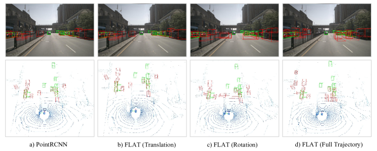
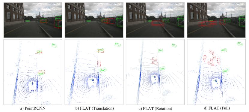
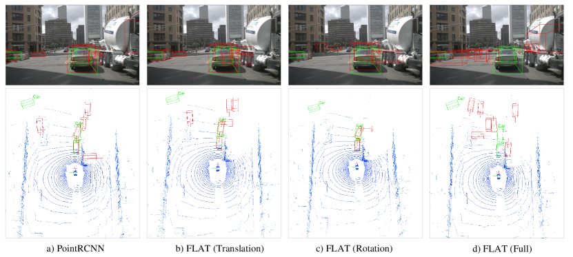
To explore the vulnerability of different stages and branches in PointRCNN, we separately attack its four modules, , classification/regression branch of stage-1/2. Qualitative results are displayed in Fig. 3 and more examples can be found in the supplementary.

Figure 3: Qualitative evaluations of white box attack. False positives are increased and output are drifted by carefully crafting the trajectory.

Table 2: Quantitative results of black box attack on nuScenes [2]: the worst and second worst performances are highlighted by red and blue color.

Category	Car	Pedes.	Barri.	Traff.	Truck	Bus	Trail.	Const.	Motor.	Bicyc.	mAP
PointPillar++ [11]	80.0	66.9	34.5	27.9	35.8	54.1	28.5	7.5	18.5	0.0	35.4
FLAT (Translation)	57.7	26.9	21.3	12.6	25.3	30.0	25.0	3.3	3.5	0.0	20.6
FLAT (Polynomial)	57.9	26.9	21.3	12.7	25.4	30.2	25.2	3.4	3.5	0.0	20.7
FLAT (Rotation)	47.7	21.1	18.6	8.9	20.2	23.5	20.5	1.7	1.3	0.0	16.4
FLAT (Full Trajectory)	45.0	18.6	16.4	5.9	18.3	22.0	19.7	1.3	0.5	0.0	14.8

Attack Translation Only. The quantitative results are exhibited in Table 1. Simply adding random noise with a small standard deviation can largely decrease the performance, , AP in the easy case is reduced by $30.44$ (around $64\%$). This phenomenon should stand as a warning for the autonomous driving community. Also, attacking classification branch of stage-2 is the most effective way to fool the detector: AP is respectively lowered by $35.72$ ($75.3\%$), $15.69$ ($72.8\%$) and $14.85$ ($71.0\%$) in the scenarios of easy, moderate and hard. This is because the stage-2 outputs the final predictions and is extremely safety-relevant. Moreover, we can find that attacking the classification branch is more effective than attacking regression, which is reasonable because classifying the objects takes priority over estimating their sizes in the detection task. Compared to the random attack, our method is more detrimental thanks to our making use of the vulnerability pointed out by the gradient. In easy, moderate, and hard scenarios, adversarial perturbation generated by attacking stage-2’s classification can yield additional drops of $5.28$, $2.71$, and $2.84$ in AP, compared to the random perturbation. Besides, our attack is better than the coordinate attack due to the parameterization, validating the superiority of the trajectory attack.

Table 3: AP of FLAT with and without regularization. $\lambda$ indicates regularization strength $\mathcal{S}$ denotes average trajectory variation and $\mathcal{D}$ denotes average point cloud distance ($\ell_{p}$ norm and Chamfer distance).

Regularization	$\lambda$	$\mathcal{S}$/$\mathcal{D}$	AP
			Easy	Moderate	Hard
Trajectory	0	0.18	0.19	0.01	0.02
	0.01	0.17	0.28	0.04	0.02
$\ell_{p}$ norm/Chamfer	0	27.54/28.70	0.19/0.19	0.01/0.01	0.02/0.02
	0.01	14.43/13.85	5.66/3.11	2.45/1.33	2.65/1.38
	0.1	2.35/3.54	21.84/14.59	9.98/6.45	9.75/ 6.59
	1	0.95/2.04	23.65/19.19	11.22/9.21	11.33/9.40

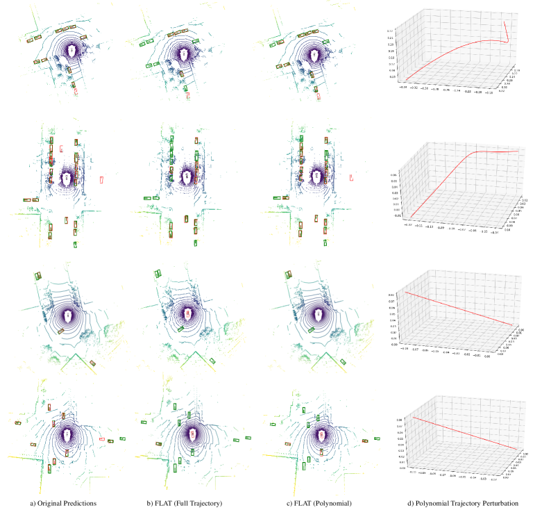
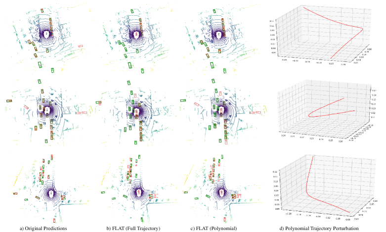
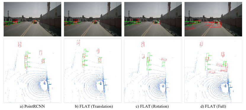
Polynomial Trajectory Perturbation. When attacking polynomial coefficients instead of the individual trajectory point, the performance is still on par with the discrete setting, as shown in Table 1, yet the attack is highly imperceptible especially in the point cloud space as shown in Fig. 4.

Figure 4: Point cloud visualization and qualitative results of black box attack. a) Raw detections of the original detector PointPillar++ [11]. b) The output of the detector after attacking the full trajectory. c) The output of the detector after polynomial trajectory perturbation in the euclidean space. d) The polynomial translation perturbation visualized in $xyz$ space, the units of three axes are all meters. Green/red boxes denote the ground truth/prediction.

Attack Rotation Only. Coordinate attack is manipulating each point’s xyz position. In contrast, our method treat each LiDAR packet as a rigid body, therefore we can attack the rotation. From Table 1 we can find that attacking classification in stage-2 is still the most powerful way to fool PointRCNN. Besides, attacking rotation achieves more performance drop compared to attacking translation, , in easy, moderate, and hard situations, AP is respectively decreased by $45.09$ ($95.0\%$), $20.76$ ($96.3\%$) and $20.30$ ($97.1\%$) in comparison with original PointRCNN. Moreover, fooling regression in stage-1 achieves the second best attacking quality, proving the effectiveness of attacking the fundamental proposal generation. Besides, attacking regression of stage-2 has the worst attacking quality, proving that attacking the refinement of box size has no significant effect. Compared to the random attack, attacking stage-2’s classification has realized additional AP drop ($9.95$, $4.07$, $4.52$), validating the merits of adversarial learning.

Attack Full Trajectory. As shown in Table 1, fooling the full trajectory has achieved the best attacking quality, , while attacking classification of stage-2, AP can be decreased to nearly zero. Compared to original PointRCNN, AP is respectively lowered by $47.25$ ($99.6\%$) in easy scenarios, indicating that the detector is completely blinded.

Attack with Regularization. As shown in Table 3, for regularizing trajectory smoothness, average trajectory variation is slightly lowered and the performance is still on par with attacking without regularization. For regularizing point cloud change, when $\lambda=0.01$, point distance is decreased by $47.6\%$ ($\ell_{p}$ norm) and $51.7\%$ (Chamfer distance), while the APs in three scenarios are still very low, thus an advanced imperceptible attack can be realized with regularization. Qualitative examples are in the supplementary.

5.5 Black Box Attack

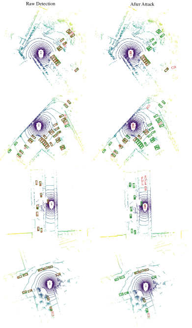
We choose voxel-based PointPillar++ [11] to test the transferability across different input representation. The quantitative results on ten categories are shown in Table 2: the performance is still largely dropped by our attack, , mAP on ten categories can be reduced by $20.6$ ($58.2\%$), and the AP on car is decreased by $35.0$ ($43.8\%$). Meanwhile, our method has demonstrated satisfactory transferability across categories. With only adversarial learning against the car detector, the detection of other categories are also deceived. For small object like pedestrian/motorcycle, AP can be dropped by $48.3$ ($72.2\%$)/$18.0$ ($97.3\%$), which has demonstrated the superior attacking quality of our method against small object detector. This superiority is mainly because the small object with less points is more susceptible to the perturbation compared to the large object like bus (dropped by $32.1$, $59.3\%$) or truck (dropped by $17.5$, $48.9\%$). Several qualitative examples are displayed in Fig. 4 and more examples are in the supplementary.

6 Conclusion

We proposed a generic and feasible DNN attack pipeline based on the trajectory against LiDAR perception. We conduct experiments on the well-studied 3D object detection task. In white box attack, even only with a 10cm perturbation in translations, the precision can be dropped by around 70$\%$. While attacking the full trajectory, the precision can be decreased to nearly zero, yet the attack is less perceptible (especially the point clouds). Our attack also shows good transferability across various input representations and target categories, raising a red flag for perception systems using LiDAR and DNN jointly.

Acknowledgment. The research is supported by NSF FW-HTF program under DUE-2026479. The authors gratefully acknowledge the useful comments and suggestions from Yong Xiao, Wenxiao Wang, Chenzhuang Du, Wang Zhao, Ziyuan Huang, Hang Zhao and Siheng Chen, and also thank Yan Wang, Shaoshuai Shi and Peiyun Wu for their helpful open-source code.

Appendix

I Overview

In the supplementary, we first present more results of our FLAT attack against black box PointPillar++ [11]. Then more qualitative evaluations of white box attack are shown, and the performances under different parameters (the number of attack iteration, the step size for each iteration, and the interpolation step) are discussed. Finally, more examples of polynomial trajectory perturbation (including both the point cloud after our attack and and the trajectory perturbation) are presented to validate the imperceptibility in point cloud space and the strong smoothness in trajectory.

II Black Box Attack

II.1 Qualitative Evaluation

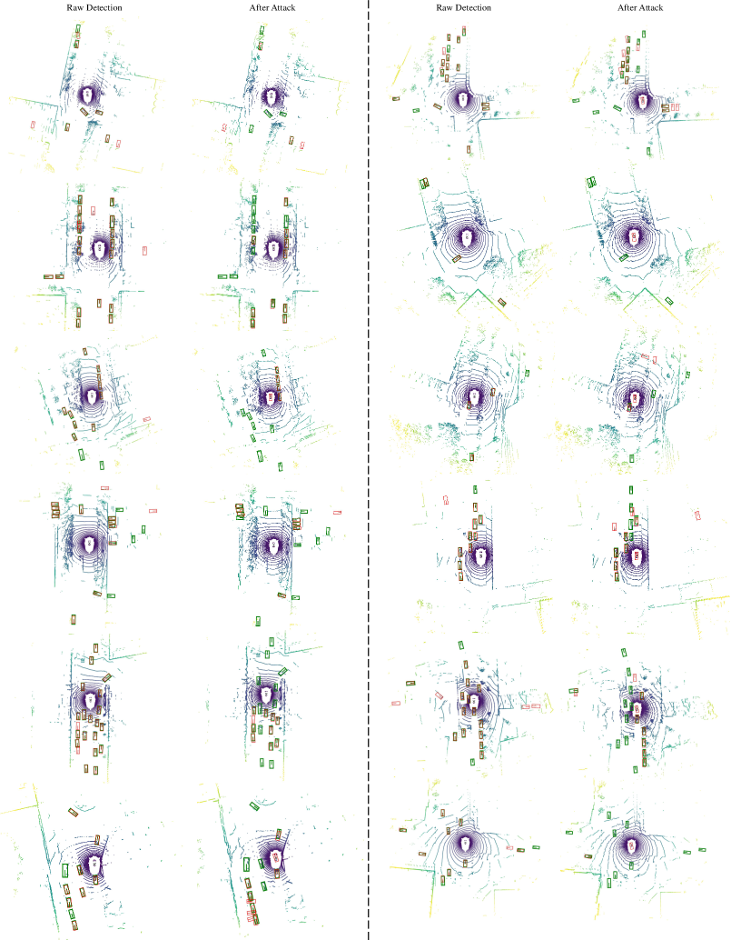
Additional qualitative examples are presented in Fig. I and Fig. II. Although our FLAT attack cannot know the model parameters of PointPillar++, a subtle perturbation can make the detector lose many safety-critical objects, , as for the four sweeps in Fig. I, the adversarial perturbation in the full trajectory can make the detector lose 7, 20, 8 and 6 objects respectively (from top to bottom), severely damaging the self-driving car’s perception module. Moreover, false positives are also increased by our perturbation (6 more in the third row of Fig. I), making the car mistakenly believe that there are obstacles in the free space.

II.2 Quantitative Evaluation

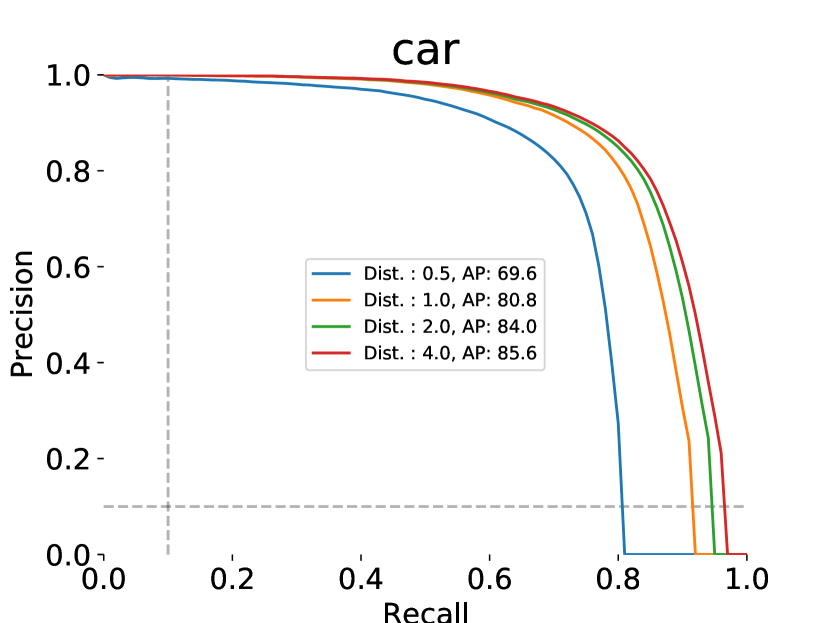
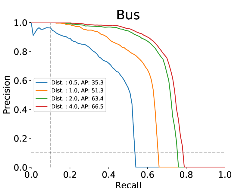
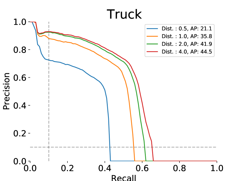
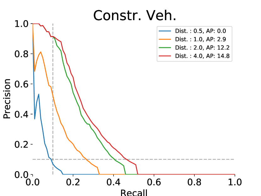
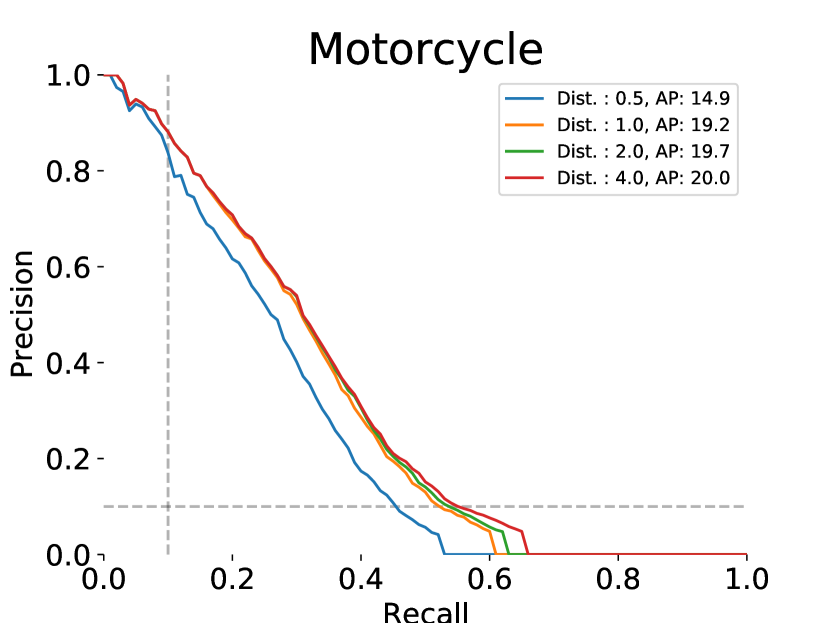
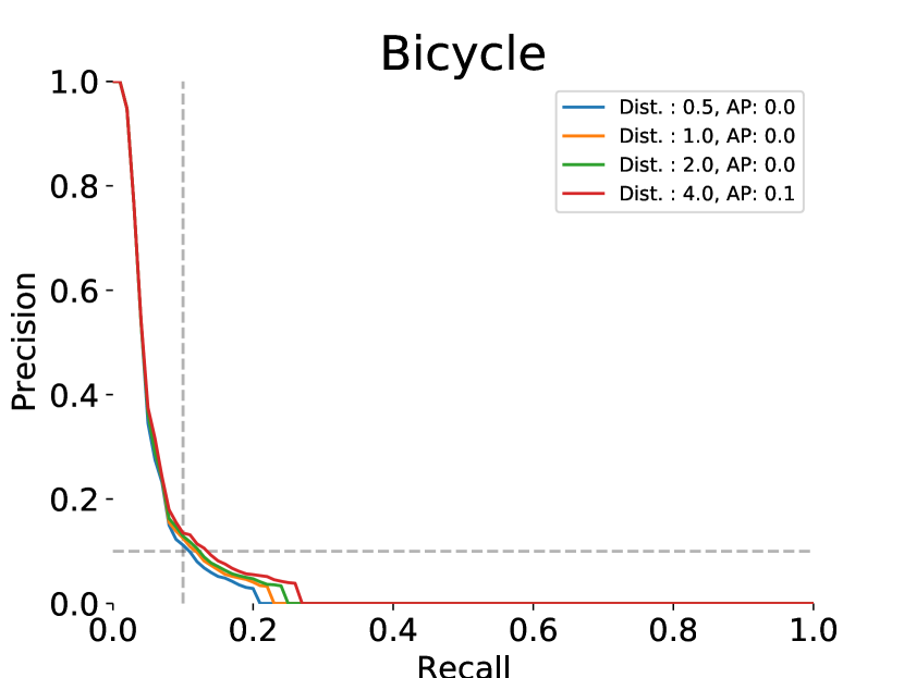
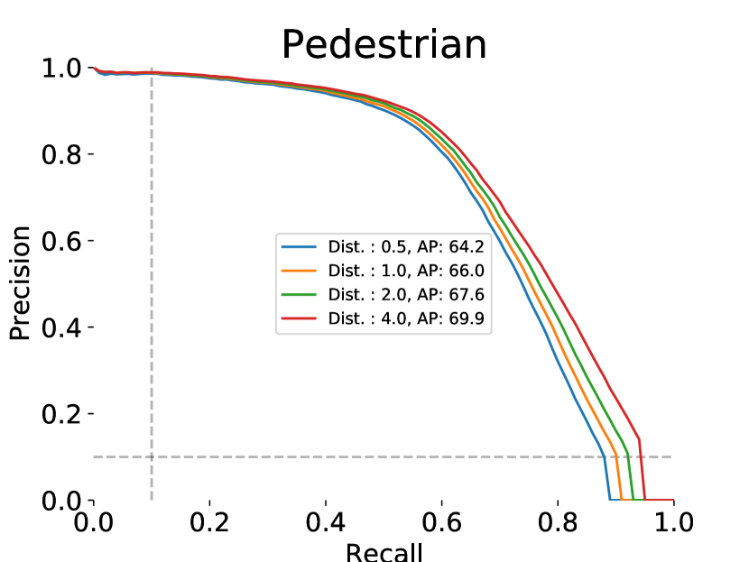
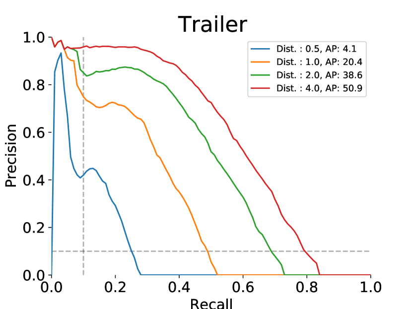
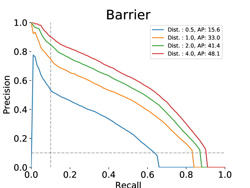
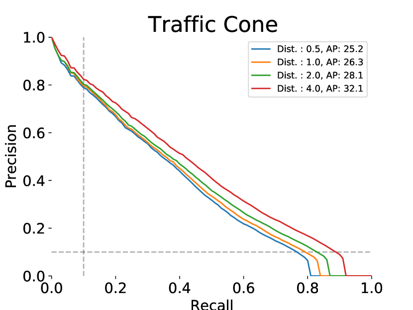
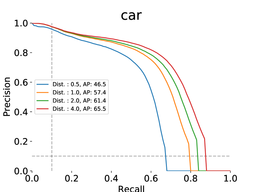
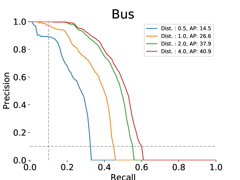
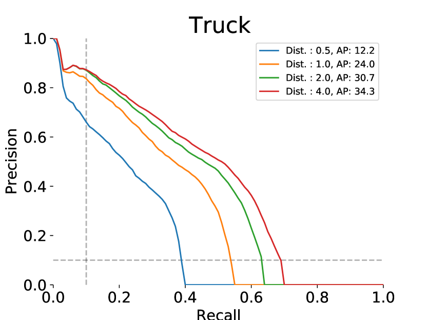
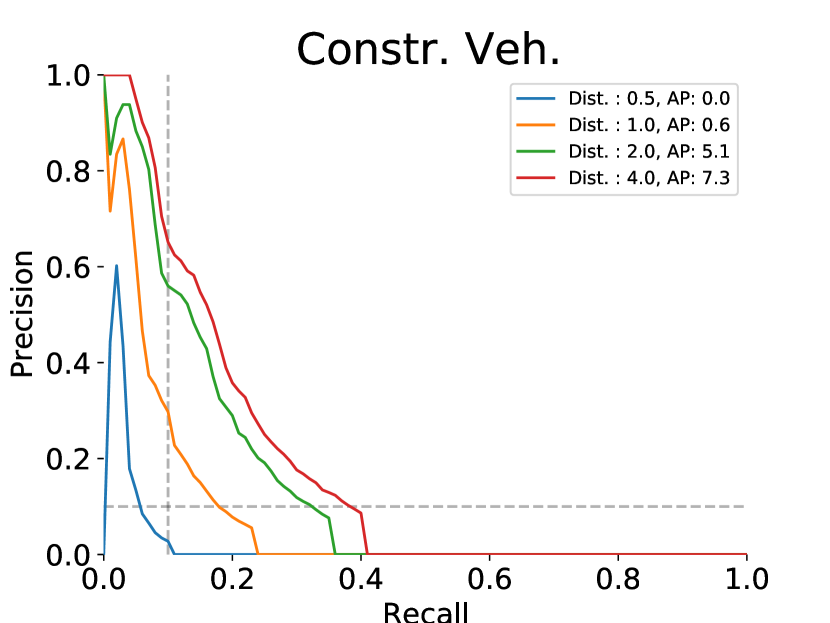
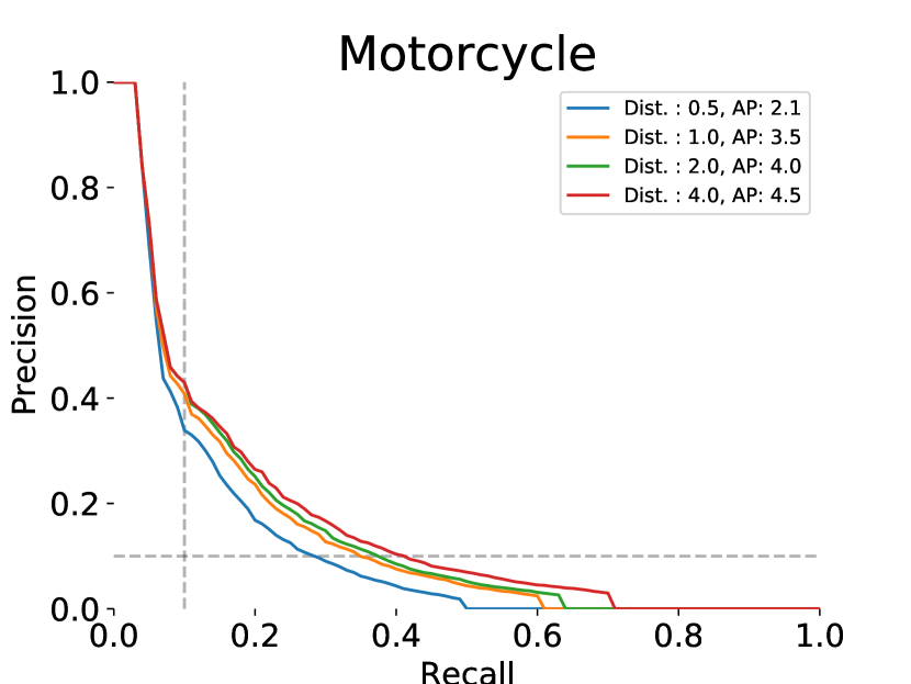
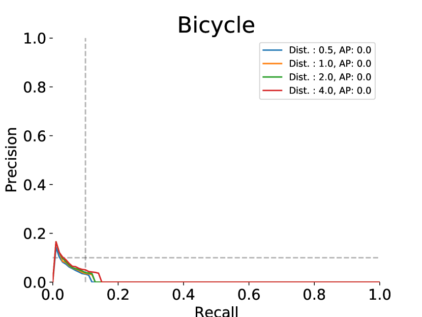
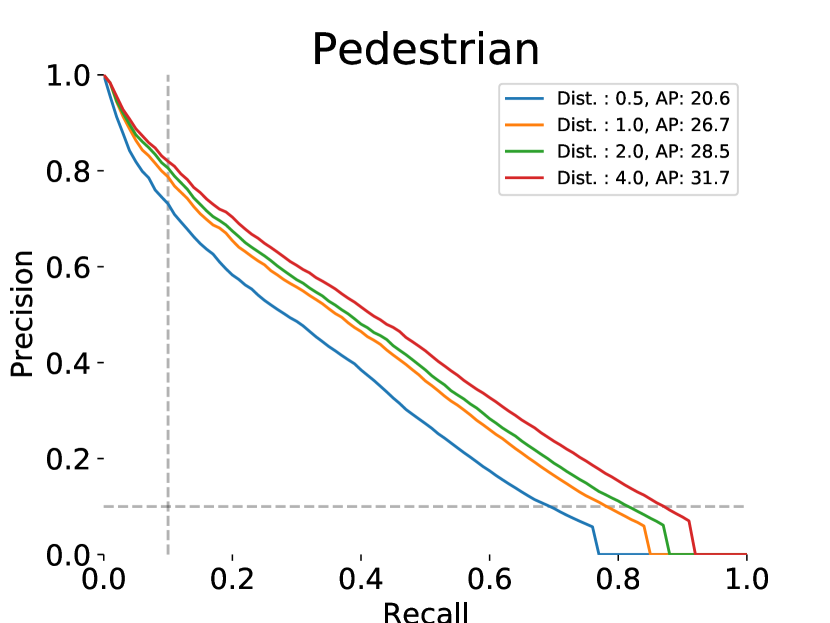
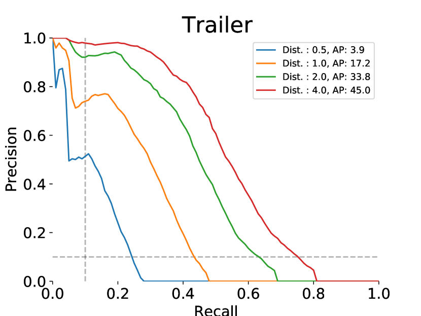
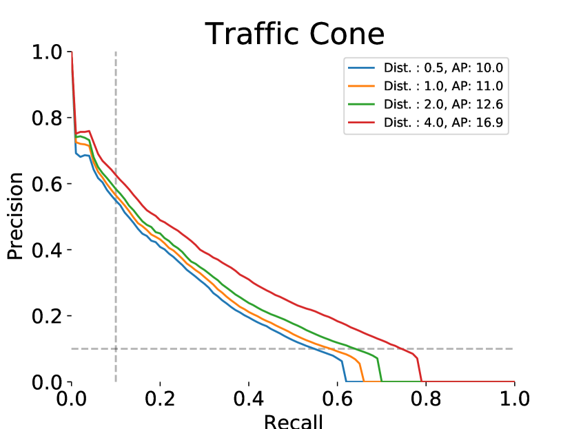
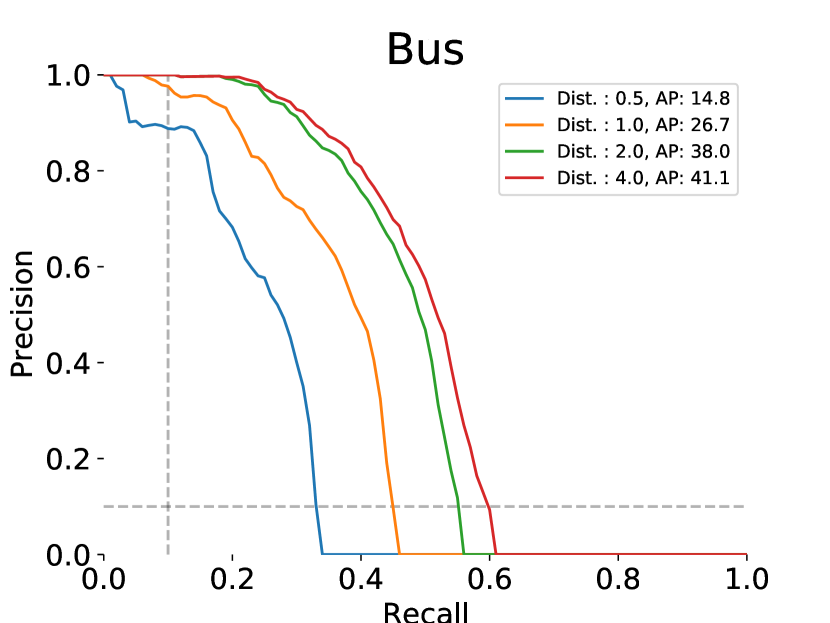
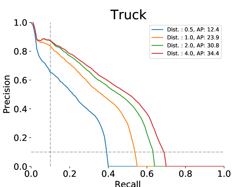
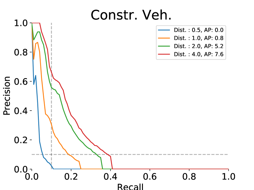
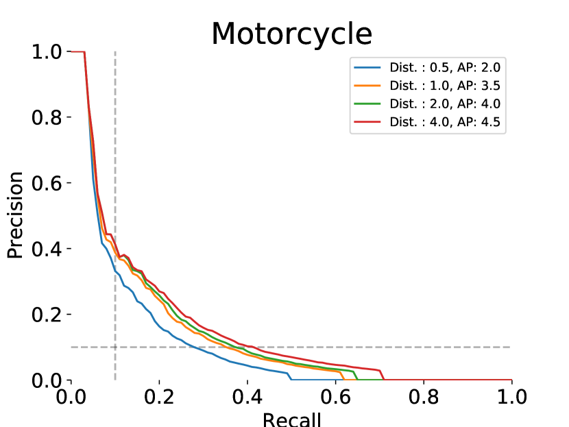
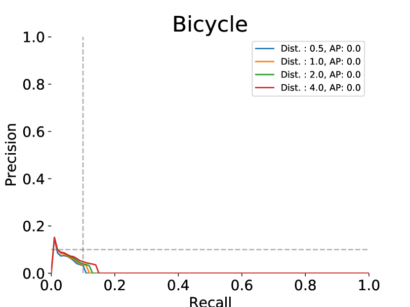
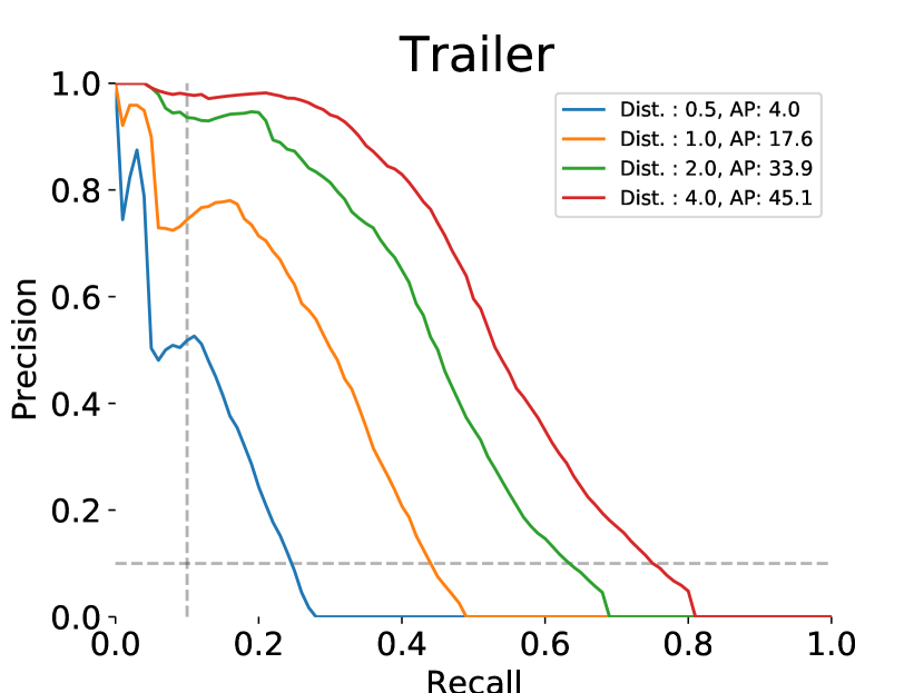
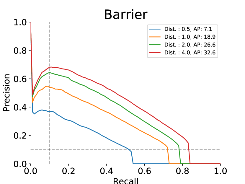
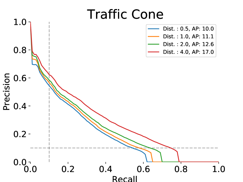
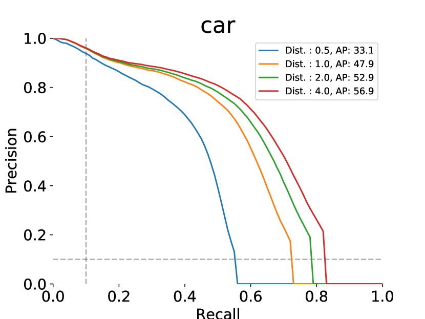
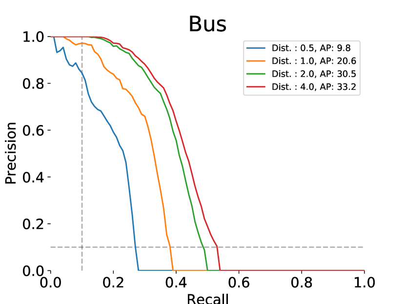
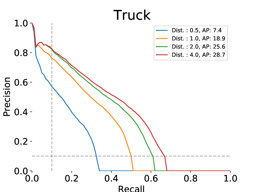
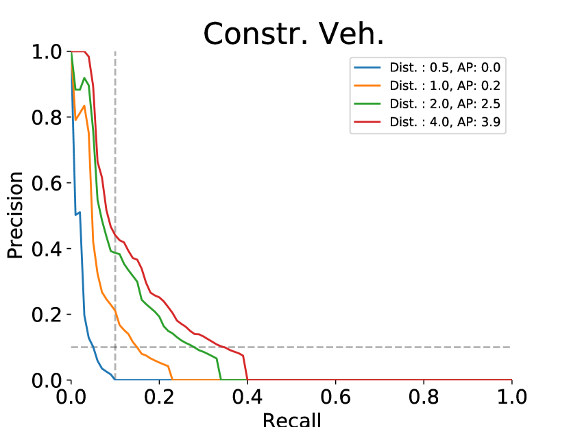
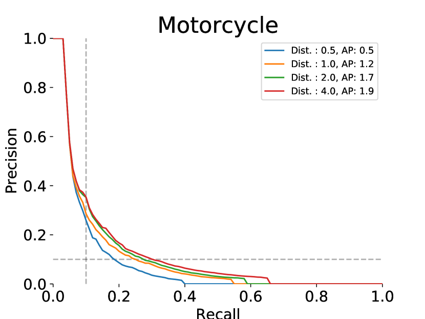
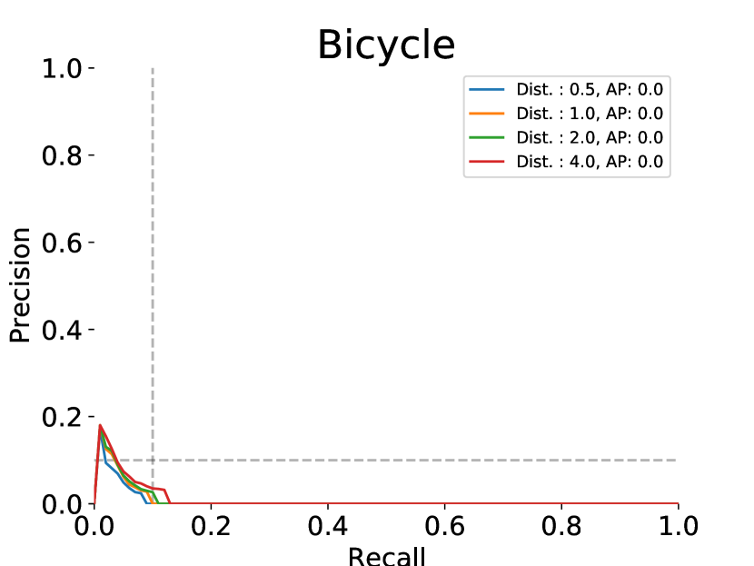
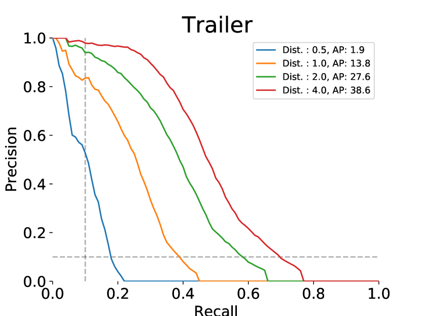
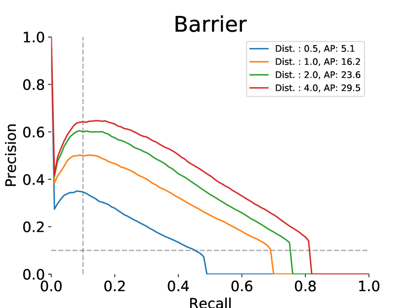
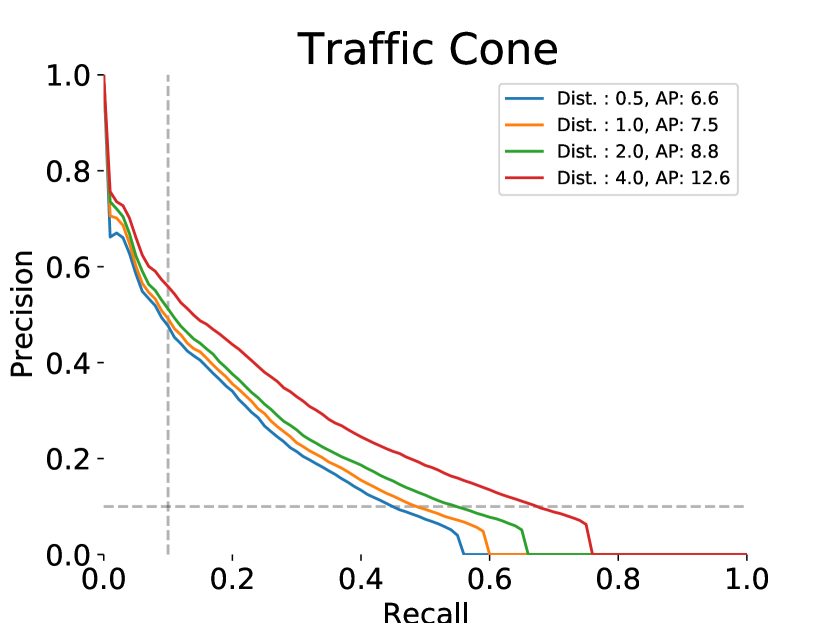
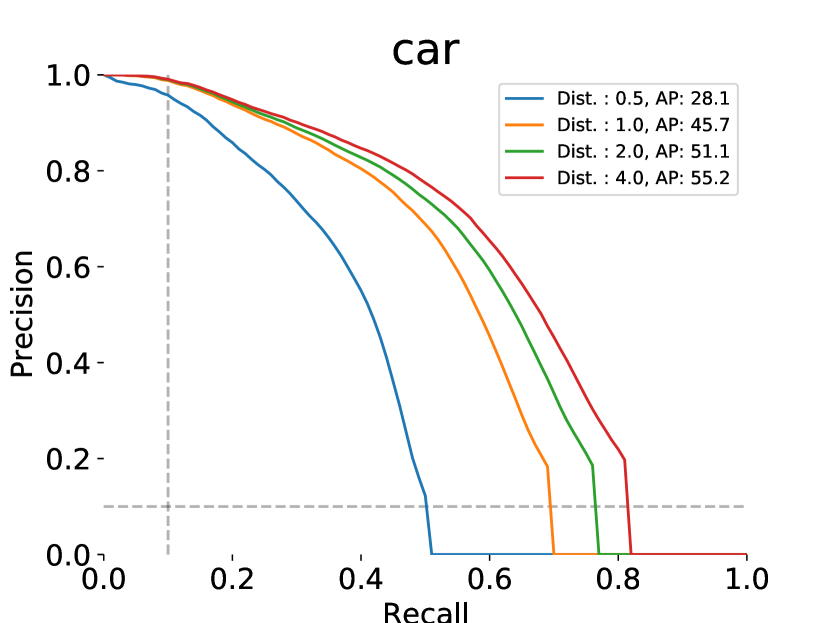
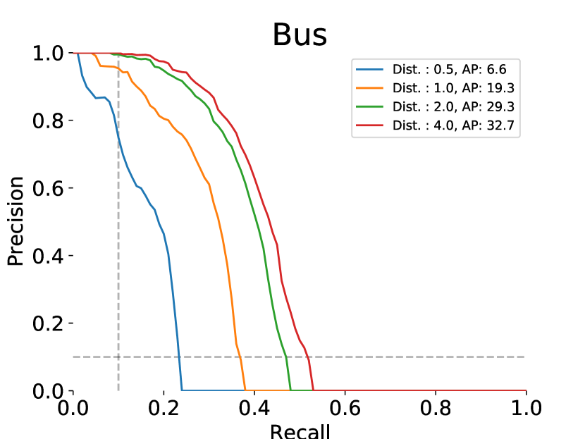
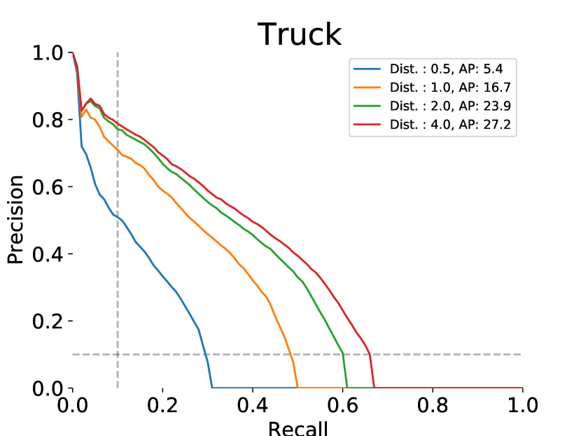
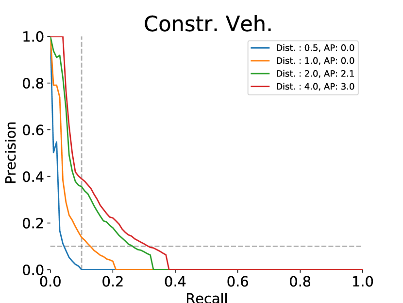
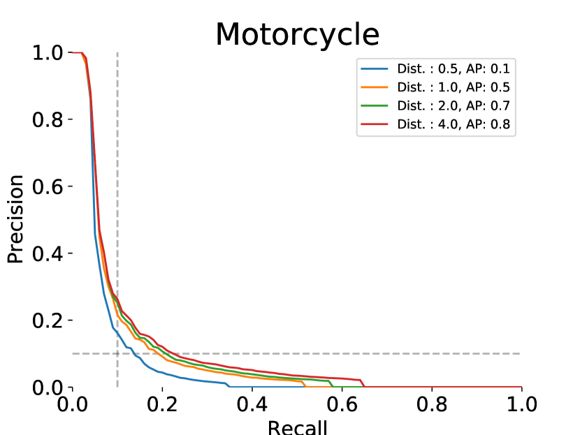
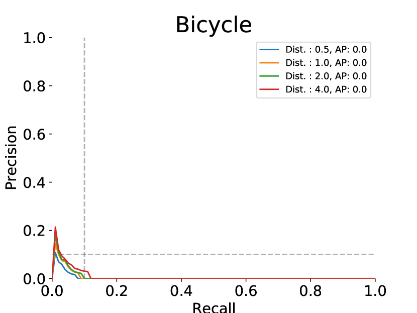
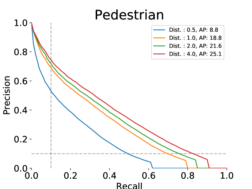
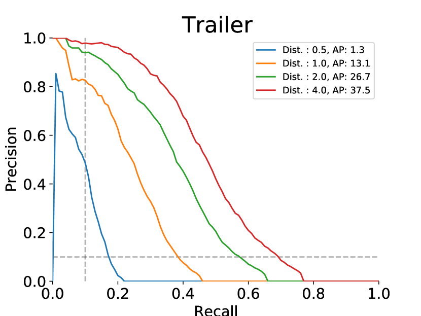
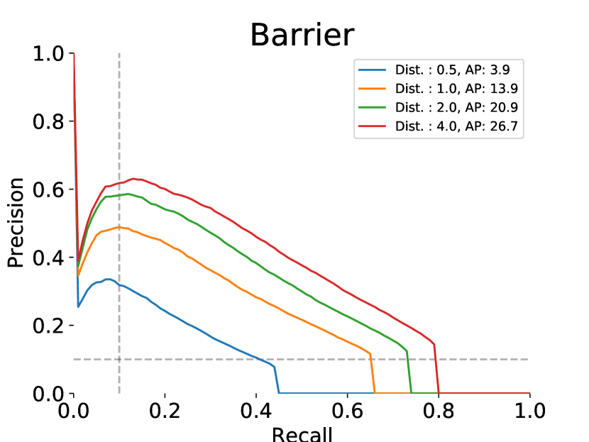
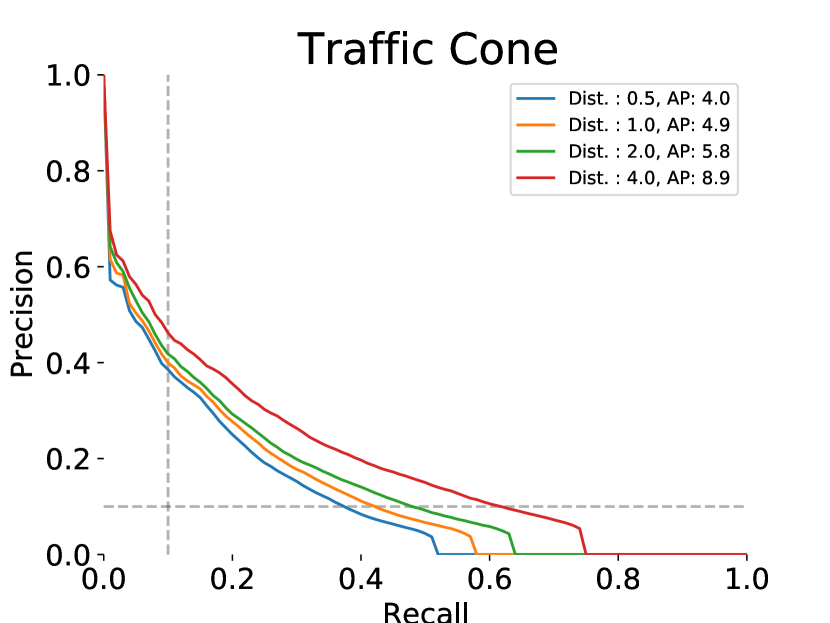
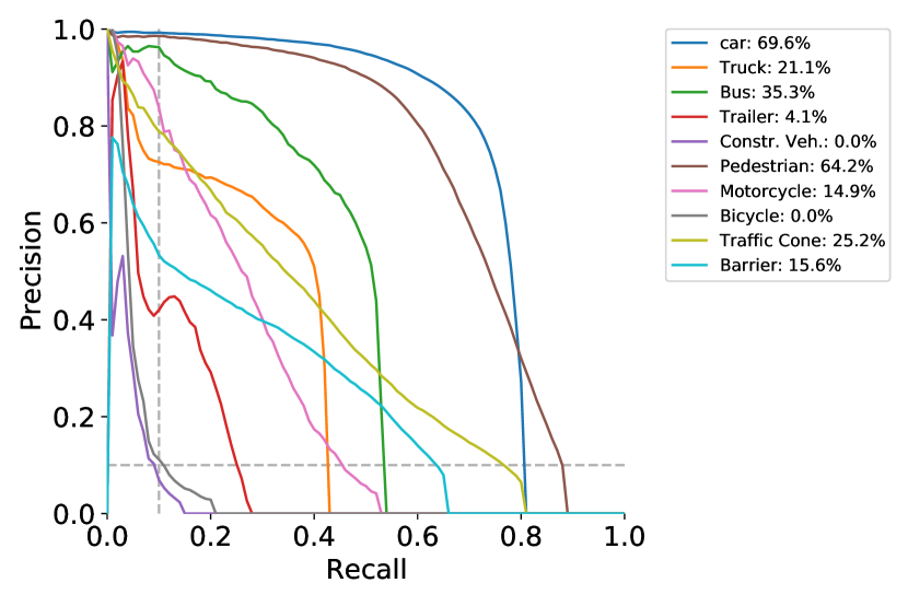
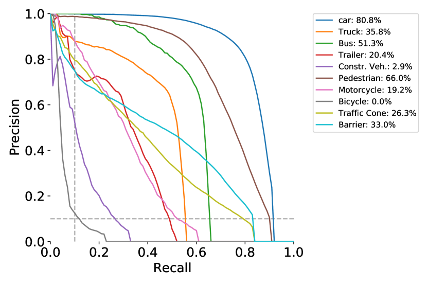
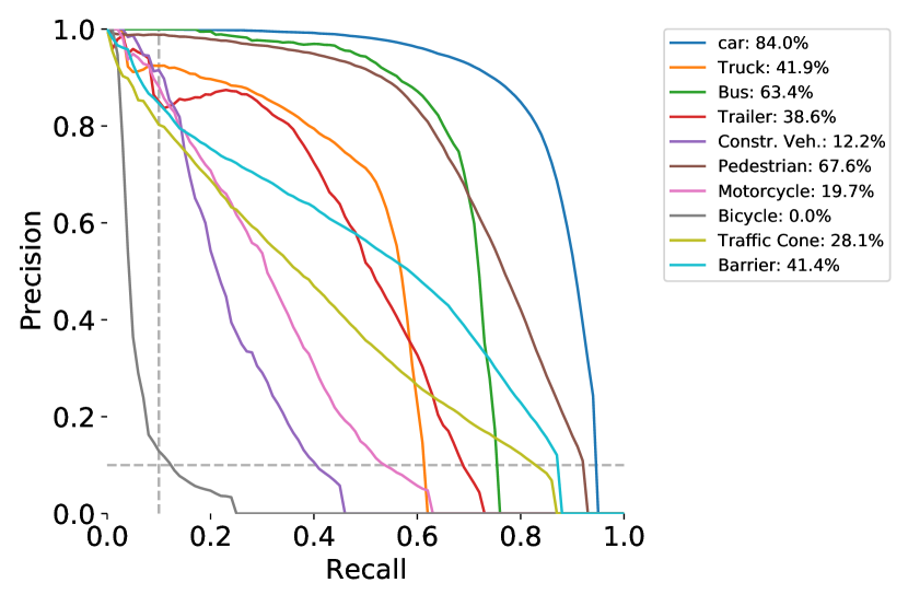
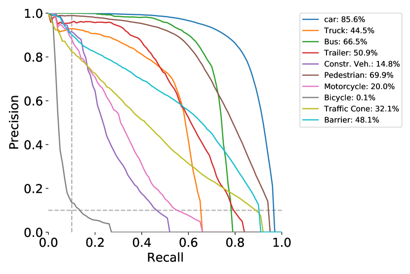
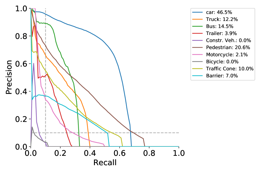
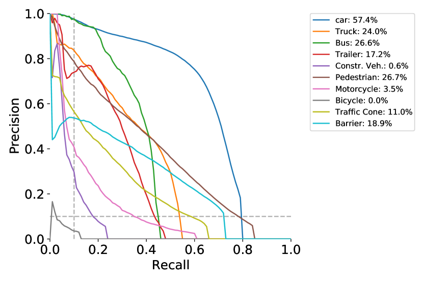
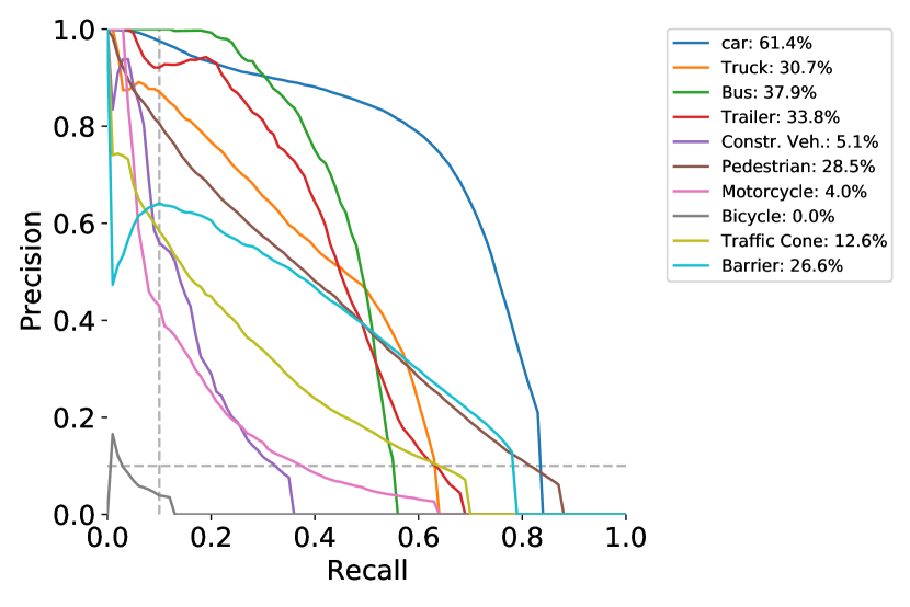
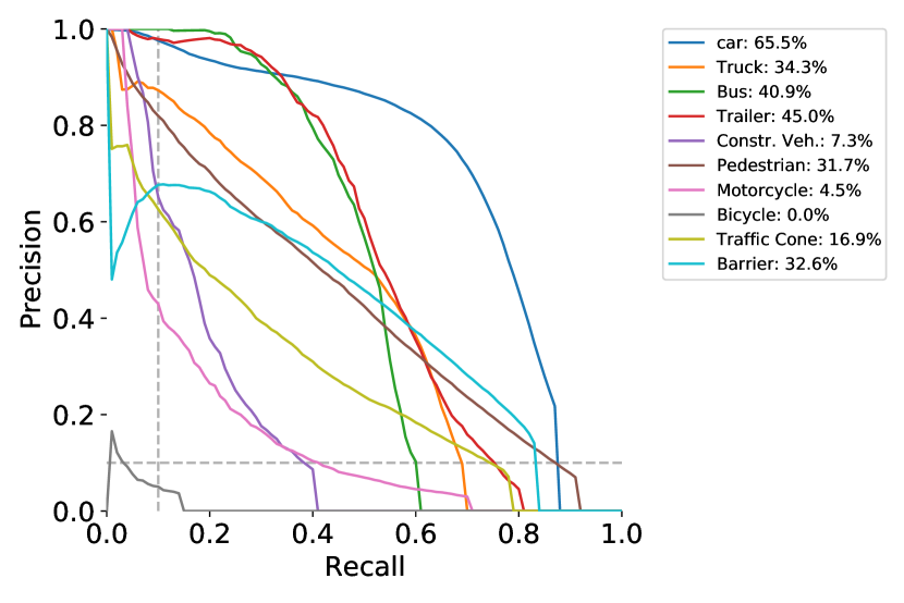
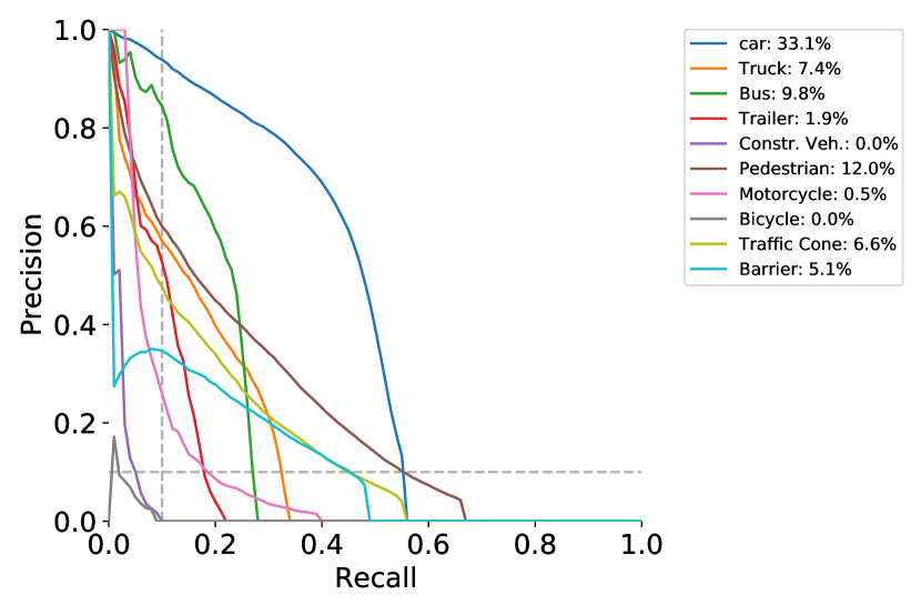
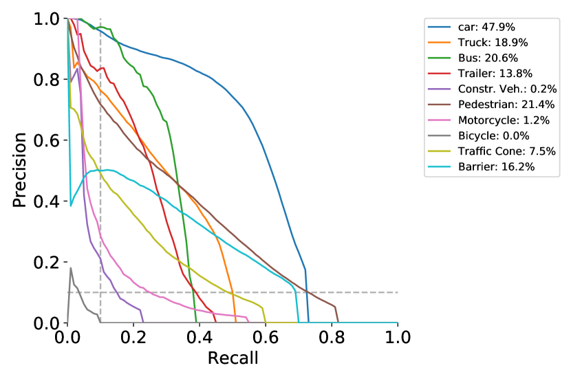
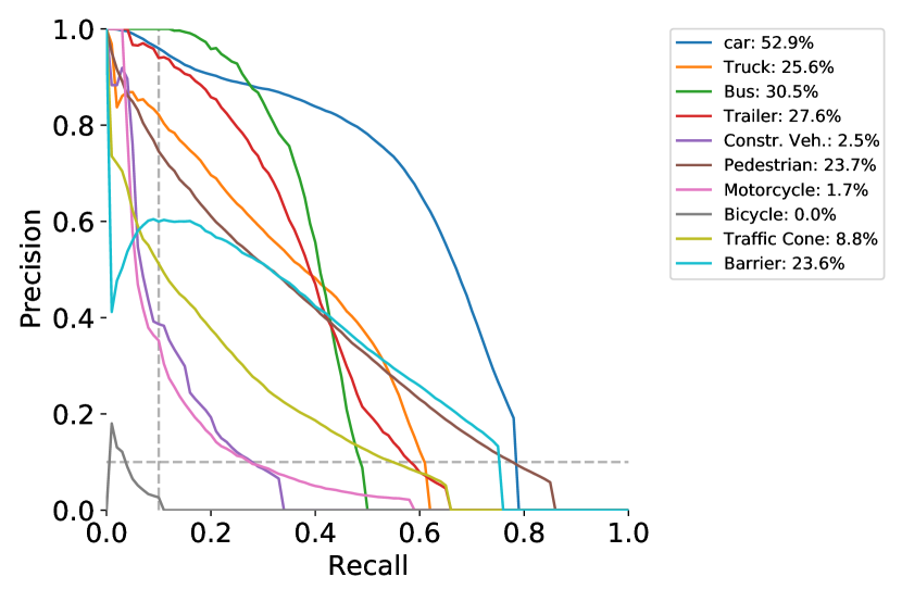
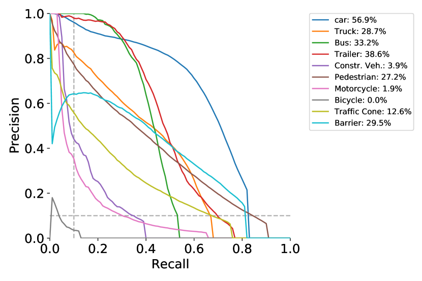
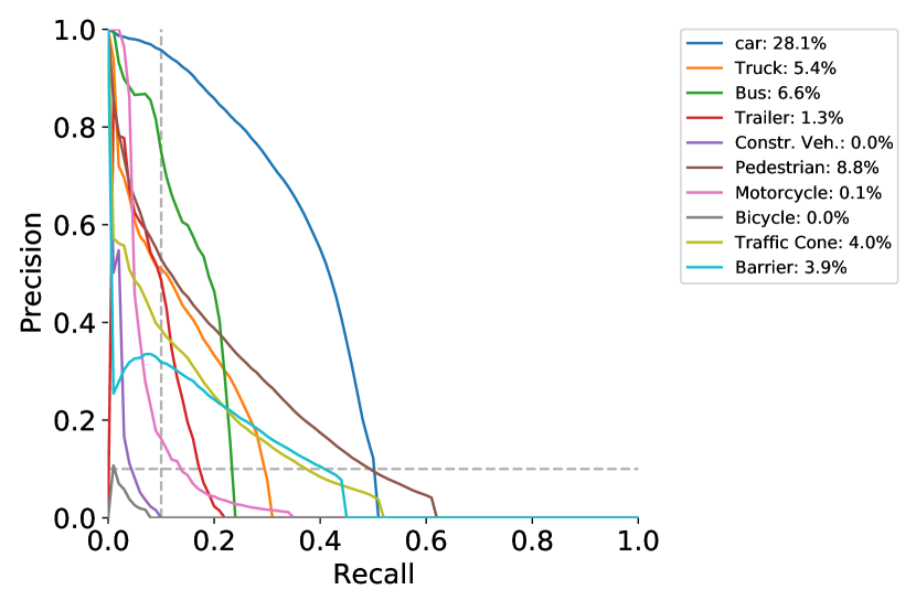
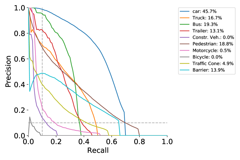
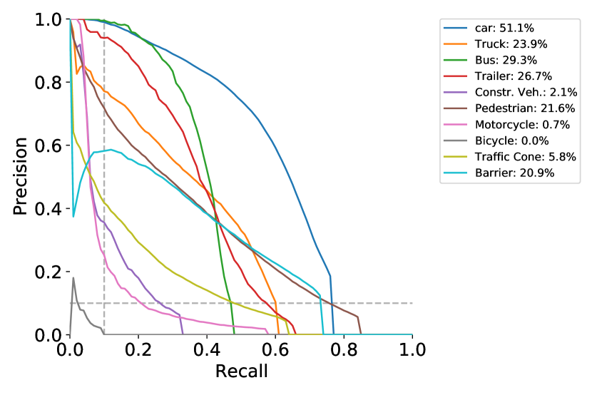
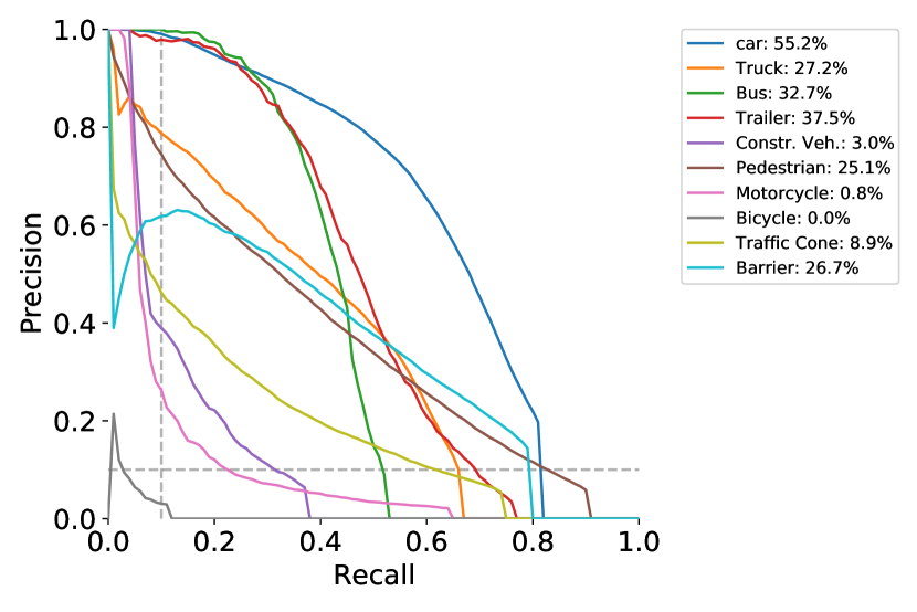
The nuScenes dataset [2] employs 2D center distance (0.5, 1, 2, 4 meters) as the matching threshold when calculating the Average Precision (AP). The per category precision-recall plots of the original detector as well as four attack settings are shown from Fig. III - Fig. VII. The performance drop is the largest when the threshold is 0.5m (the highest precision standard), , the AP@0.5m in car category is decreased by $23.1$($33.1\%$), $36.5$($52.4\%$), $41.5$($59.6\%$) while attacking translation, rotation and the full trajectory. As shown in Fig. VIII, the curve shifts to the lower left when increasing the attack magnitude.

Figure I: Qualitative results of black box attack when attacking the full trajectory. The left and right figures are respectively original and distorted LiDAR sweep as well as the detection results. Green/red boxes denote the ground truth/prediction respectively.

Figure II: Qualitative results of the black box attack when attacking the full trajectory. Green/red boxes denote the ground truth/prediction respectively.

(a) t

(b) t

(c) t

(d) t

(e) t

Figure III: Per category precision-recall plot of PointPillar++ on the nuScenes validation set [2].

(a) t

(b) t

(c) t

(d) t

(e) t

Figure IV: Per category precision-recall plot of attacking the translation only (black box) on the nuScenes validation set [2].

(a) t

(b) t

(c) t

(d) t

(e) t

Figure V: Per category precision-recall plot of attacking the polynomial coefficients (black box) on the nuScenes validation set [2].

(a) t

(b) t

(c) t

(d) t

(e) t

Figure VI: Per category precision-recall plot of attacking the rotation only (black box) on the nuScenes validation set [2].

(a) t

(b) t

(c) t

(d) t

(e) t

Figure VII: Per category precision-recall plot of attacking the full trajectory (black box) on the nuScenes validation set [2].

(a) t

(b) t

(c) t

(d) t

Figure VIII: Per category precision-recall plot of original detector, attacking translation only, attacking rotation only, attacking full trajectory (black box) on the nuScenes validation set [2] (from left to right). From top to bottom is respectively the results from four thresholds (0.5m, 1.0m, 2.0m, 4.0m). From left to right, the curve shifts to the lower left when increasing the attack magnitude.

III White Box Attack

III.1 Qualitative Evaluation

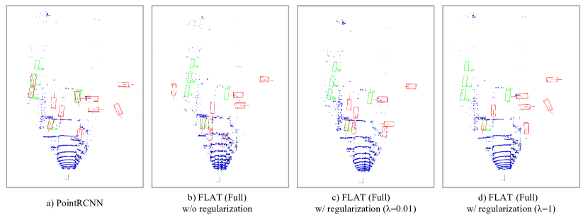
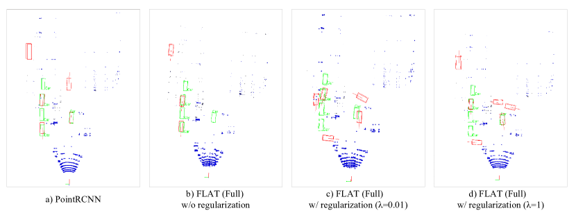
Three qualitative examples are demonstrated in Fig. IX - Fig. XI. In Fig. IX, original PointRCNN can perceive three our of five cars, and attacking translation only has slightly shifted the predictions. Attacking rotation has a stronger impact and cause two objects to be undetectable, while attacking the full trajectory further creates four false positives. In Fig. X, PointRCNN can successfully detect two out of three surrounding cars, then adversarial translation perturbation make the detection of the nearest car drift. Both two detections are drifted in the scenario of adversarial rotation perturbation. Finally, when attacking both translation and rotation, five false positives have emerged, severely degrading the perception capability of the self-driving car. Similar results can be found in Fig. XI. Moreover, three qualitative examples of attacking with and without regularization are presented in Fig. XII, Fig. XIII and Fig. XIV. As the strength of regularization is enlarged, the variation in the point space is reduced, enabling less perceptible attack.

III.2 Different Parameters

The detection performances under different parameter settings are reported in Table I - Table III. In the case of attacking the translation (fooling classification in stage-2), AP of easy case in six parameter settings fluctuate between $11.72$ and $13.89$, which means that all the parameter configurations can produce a high-quality adversarial perturbation. In the situation of attacking the full trajectory (with the aim of attacking regression branch in stage-1), AP of easy case in six parameter settings fluctuate between $0.53$ and $2.44$, proving that all the six settings can maintain the attacking quality at a high level. To sum up, the number of iteration and the step size for each iteration has a relatively small impact on our FLAT attack. As for the interpolation step, when it is increased, there will be more sectors, , more point cloud groups, and the number of trajectory points which can be attacked are also increased, easing the learning of an effective adversarial perturbation. Consequently, when the interpolation step is increased from 50 to 1000, the AP in easy scenarios can be lowered by $5.04$ ($36.7\%$) while attacking the translation, by $3.70$ ($78.2\%$) while attacking the rotation, and by $0.51$ ($87.9\%$) while attacking the full trajectory, as shown in Table IV.

Noted that our simulation of motion distortion/correction accurately matches with the real-world scenarios, , in Fig. 2 of [29]: “the Velodyne VLP-16 software used in our electric vehicle platform produces 76 packets for each full revolution scan. Each packet covers an azimuth angle of approximately $4.74^{\circ}$.” Noted that the number of point cloud sector/packet is adjustable depending on vehicle platforms, and the attack performance keeps at a high level under different number of sector/interpolation step, as shown in Table IV.

IV Polynomial Trajectory Perturbation

Our trajectory attack is feasible, , through GNSS spoofing as proven in [23]: “Today, it is feasible to execute GNSS spoofing attacks with less than $\$100$ of equipment. GNSS signal generators can be programmed to transmit radio frequency signals corresponding to a static position, or simulate entire trajectories.” We have verified the effectiveness of the discrete adversarial trajectory perturbation in both white box and black box attack. To achieve a temporally-smooth attack which is less perceptible, we implement a polynomial regression before the generation of perturbation and attack the polynomial coefficients instead of the trajectory itself. In this scenario, we only need to manipulate several key points to bend a polynomial-parameterized trajectory which can be easily achieved in reality, realizing a real-time and high-quality attack. Several qualitative examples of the polynomial trajectory perturbation are shown in Fig. XV. Although the attack performance is inferior to the full trajectory attack, the detector still missed many safety-critical objects yet the perturbation in point cloud space is highly imperceptible: even for human eyes, it is quite difficult to distinguish the point cloud before and after the polynomial trajectory perturbation.

V Summary

In this supplementary, we presented more qualitative evaluations of both white box and black box attack, to validate the effectiveness of our attack pipeline. Besides, we found that the number of PGD iteration and the step size for each iteration have a relatively small impact on the attack quality, but the interpolation step, , the number of LiDAR packets, can have a relatively large influence on the attack performance, because increasing trajectory points which can be deliberately modified can facilitate the adversarial learning, resulting in a stronger adversarial perturbation. Finally, more qualitative examples of the polynomial trajectory perturbation are demonstrated to validate the imperceptibility of out attack.

Figure IX: Qualitative evaluations of white box attack. False positives are increased and predictions are drifted by carefully crafting the vehicle trajectory.

Table I: 3D detection performance of white-box translation attack. We report the average precision of the 3D bounding box for the car category with the IoU threshold 0.7, under different levels of difficulty and ranges of depth following [28]. iter_eps and nb_iter respectively denote the step size of each iteration and the number of iteration. The best and second best attack qualities are respectively highlighted using red and blue color.

Attack Setting  $\backslash$  Case		iter_eps	nb_iter	Easy	Moderate	Hard	0-30m	30-50m	50-70m
None		-	-	47.44	21.56	20.91	47.44	2.16	0.17
Coordinate Attack		-	-	16.42	6.58	5.90	15.20	0.48	0.03
Random Attack		-	-	17.00	8.58	8.90	20.43	1.09	0.09
Classification	Stage-1	0.05	10	15.38	7.32	7.66	18.12	0.93	0.03
		0.05	20	16.85	8.49	8.69	19.87	1.29	0.05
		0.05	30	17.60	8.81	8.95	20.60	0.82	0.05
		0.1	10	13.12	6.49	6.79	15.83	0.71	0.04
		0.1	20	12.94	6.58	7.22	16.82	0.86	0.06
		0.1	30	14.77	7.14	7.69	18.57	0.74	0.05
	Stage-2	0.05	10	12.47	6.72	7.29	16.13	1.16	0.14
		0.05	20	13.89	6.82	6.96	16.11	0.95	0.17
		0.05	30	11.87	5.98	6.40	14.87	0.67	0.05
		0.1	10	12.58	6.40	6.77	15.25	0.95	0.07
		0.1	20	11.72	5.87	6.06	13.91	0.87	0.04
		0.1	30	12.54	6.52	6.69	15.14	0.96	0.09
Regression	Stage-1	0.05	10	17.45	8.43	8.42	19.53	1.12	0.04
		0.05	20	16.52	8.53	8.75	19.69	1.37	0.04
		0.05	30	17.60	8.81	9.11	21.19	0.85	0.04
		0.1	10	14.47	7.51	7.88	17.77	1.07	0.05
		0.1	20	17.46	8.24	8.57	19.36	1.09	0.03
		0.1	30	14.42	7.04	7.31	16.44	1.02	0.13
	Stage-2	0.05	10	26.07	12.76	12.51	27.19	2.16	0.17
		0.05	20	26.05	12.75	12.50	27.19	2.16	0.15
		0.05	30	26.07	12.76	12.51	27.19	2.16	0.17
		0.1	10	26.07	12.76	12.51	27.19	2.16	0.17
		0.1	20	26.09	12.78	12.53	27.15	2.17	0.17
		0.1	30	26.07	12.76	12.51	27.19	2.16	0.17

Figure X: Qualitative evaluations of white box attack. False positives are increased and predictions are drifted by carefully crafting the vehicle trajectory.

Table II: 3D object detection performance of white-box rotation attack. Other settings are similar to Table I.

Attack Setting  $\backslash$  Case		iter_eps	nb_iter	Easy	Moderate	Hard	0-30m	30-50m	50-70m
None		-	-	47.44	21.56	20.91	47.44	2.16	0.17
Random Attack		-	-	12.30	4.87	5.13	13.31	0.01	0.00
Classification	Stage-1	0.005	10	5.38	1.91	2.05	5.89	0.01	0.00
		0.005	20	7.16	2.94	2.81	7.75	0.02	0.00
		0.005	30	6.17	2.41	2.49	7.02	0.01	0.00
		0.01	10	3.93	1.70	1.61	4.79	0.01	0.00
		0.01	20	6.32	2.43	2.51	7.32	0.02	0.00
		0.01	30	6.83	2.53	2.27	6.87	0.02	0.00
	Stage-2	0.005	10	4.32	1.48	1.35	4.08	0.00	0.00
		0.005	20	3.39	1.20	1.14	3.39	0.01	0.00
		0.005	30	6.59	2.22	2.04	6.15	0.01	0.00
		0.01	10	3.18	1.20	1.17	3.44	0.00	0.00
		0.01	20	2.35	0.80	0.61	2.03	0.01	0.00
		0.01	30	2.36	0.90	0.94	2.84	0.01	0.00
Regression	Stage-1	0.005	10	8.46	3.56	3.36	9.01	0.04	0.00
		0.005	20	8.11	3.11	3.06	7.96	0.02	0.03
		0.005	30	8.03	3.25	3.02	8.27	0.01	0.00
		0.01	10	5.02	1.79	1.61	4.79	0.01	0.01
		0.01	20	5.50	1.87	1.76	5.45	0.02	0.00
		0.01	30	4.17	1.53	1.47	4.60	0.01	0.00
	Stage-2	0.005	10	25.99	12.71	12.49	27.07	2.16	0.17
		0.005	20	26.07	12.76	12.51	27.19	2.16	0.17
		0.005	30	26.07	12.76	12.51	27.19	2.16	0.17
		0.01	10	26.07	12.76	12.51	27.19	2.16	0.17
		0.01	20	26.30	12.89	12.59	27.35	2.17	0.17
		0.01	30	26.18	12.75	12.53	27.24	2.16	0.17

Figure XI: Qualitative evaluations of white box attack. False positives are increased and predictions are drifted by carefully crafting the vehicle trajectory.

Table III: 3D detection performance of white-box full trajectory attack. Other settings are similar to Table I.

Attack Setting  $\backslash$  Case		iter_eps	iter_eps2	nb_iter	Easy	Moderate	Hard	0-30m	30-50m	50-70m
None		-	-	-	47.44	21.56	20.91	47.44	2.16	0.17
Random Attack		-	-	-	5.66	2.43	2.78	7.67	0.02	0.00
Classification	Stage-1	0.005	0.05	10	1.11	0.25	0.23	1.19	0.02	0.00
		0.005	0.05	20	2.89	1.02	1.15	3.52	0.01	0.00
		0.005	0.05	30	0.65	0.21	0.25	0.88	0.01	0.00
		0.01	0.1	10	0.57	0.16	0.16	0.67	0.01	0.00
		0.01	0.1	20	1.52	0.45	0.51	1.71	0.01	0.00
		0.01	0.1	30	0.84	0.20	0.24	1.03	0.00	0.00
	Stage-2	0.005	0.05	10	0.37	0.09	0.07	0.43	0.00	0.00
		0.005	0.05	20	0.42	0.15	0.12	0.56	0.00	0.00
		0.005	0.05	30	0.09	0.01	0.02	0.12	0.00	0.00
		0.01	0.1	10	0.22	0.02	0.02	0.21	0.00	0.00
		0.01	0.1	20	0.19	0.01	0.02	0.26	0.00	0.00
		0.01	0.1	30	0.54	0.15	0.15	0.54	0.03	0.00
Regression	Stage-1	0.005	0.05	10	1.20	0.33	0.32	1.27	0.01	0.00
		0.005	0.05	20	2.44	0.90	0.88	2.72	0.02	0.00
		0.005	0.05	30	2.07	0.77	0.76	2.68	0.01	0.00
		0.01	0.1	10	0.90	0.36	0.35	1.18	0.01	0.00
		0.01	0.1	20	1.01	0.35	0.32	1.27	0.01	0.00
		0.01	0.1	30	0.53	0.11	0.13	0.80	0.03	0.00
	Stage-2	0.005	0.05	10	26.07	12.76	12.51	27.19	2.16	0.17
		0.005	0.05	20	26.08	12.76	12.52	27.19	2.17	0.17
		0.005	0.05	30	26.06	12.75	12.51	27.17	2.16	0.17
		0.01	0.1	10	26.07	12.76	12.51	27.19	2.16	0.17
		0.01	0.1	20	26.03	12.70	12.48	27.13	2.16	0.17
		0.01	0.1	30	26.07	12.76	12.51	27.19	2.16	0.17

Table IV: 3D object detection performance under different interpolation steps (attacking the classification in stage-2). The number of iteration and the step size for each iteration is fixed as 20 and 0.1/0.01 (translation/rotation), respectively.

Attack Setting	Interpolation Step	Easy	Moderate	Hard	0-30m	30-50m	50-70m
FLAT (Translation)	25	16.97	7.71	7.99	18.12	0.93	0.13
	50	13.73	4.75	6.33	16.33	0.34	0.00
	100	11.72	5.87	6.06	13.91	0.87	0.04
	500	10.29	4.64	5.94	17.35	0.73	0.00
	1000	8.69	3.02	5.52	14.62	1.10	0.00
FLAT (Rotation)	25	2.53	0.89	0.75	2.18	0.00	0.00
	50	4.73	1.66	1.59	4.30	0.01	0.00
	100	2.35	0.80	0.61	2.03	0.01	0.00
	500	1.77	0.62	0.75	2.70	0.01	0.00
	1000	1.03	0.27	0.21	1.11	0.00	0.00
FLAT (Full)	25	0.36	0.13	0.14	0.40	0.00	0.00
	50	0.58	0.18	0.17	0.58	0.00	0.00
	100	0.19	0.01	0.02	0.26	0.00	0.00
	500	0.17	0.01	0.02	0.09	0.00	0.00
	1000	0.07	0.02	0.02	0.11	0.01	0.00

Figure XII: Qualitative example of FLAT attack with and without regularization. A minor perturbation in point cloud can fool the detector.

Figure XIII: Qualitative example of FLAT attack with and without regularization. A minor perturbation in point cloud can fool the detector.

Figure XIV: Qualitative example of FLAT attack with and without regularization. A minor perturbation in point cloud can fool the detector.

Figure XV: Point cloud visualization and qualitative results of black box attack. a) Raw detections of the original detector PointPillar++ [11]. b) The output of the detector after attacking the full trajectory. c) The output of the detector after polynomial trajectory perturbation in the euclidean space. d) The polynomial translation perturbation visualized in $xyz$ space, the units of three axes are all meters.

References

- Brendel et al. [2018] W. Brendel, Jonas Rauber, and M. Bethge. Decision-based adversarial attacks: Reliable attacks against black-box machine learning models. In International Conference on Learning Representation, 2018.
- Caesar et al. [2020] H. Caesar, Varun Bankiti, A. Lang, Sourabh Vora, Venice Erin Liong, Q. Xu, A. Krishnan, Yu Pan, Giancarlo Baldan, and Oscar Beijbom. nuscenes: A multimodal dataset for autonomous driving. In IEEE Conference on Computer Vision and Pattern Recognition, pages 11618–11628, 2020.
- Cao et al. [2019] Yulong Cao, Chaowei Xiao, Benjamin Cyr, Yimeng Zhou, Won Park, Sara Rampazzi, Q. Chen, K. Fu, and Z. Morley Mao. Adversarial sensor attack on lidar-based perception in autonomous driving. In Proceedings of the ACM SIGSAC Conference on Computer and Communications Security, 2019.
- Cao et al. [2019] Yulong Cao, Chaowei Xiao, Dawei Yang, J. Fang, Ruigang Yang, M. Liu, and Bo Li. Adversarial objects against lidar-based autonomous driving systems. ArXiv, abs/1907.05418, 2019.
- Fan et al. [2017] Haoqiang Fan, H. Su, and L. Guibas. A point set generation network for 3d object reconstruction from a single image. In IEEE Conference on Computer Vision and Pattern Recognition, pages 2463–2471, 2017.
- Frossard et al. [2020] Davi Frossard, Simon Suo, S. Casas, J. Tu, Rui Hu, and R. Urtasun. Strobe: Streaming object detection from lidar packets. In 4th Conference on Robot Learning, 2020.
- Geiger et al. [2012] Andreas Geiger, Philip Lenz, and R. Urtasun. Are we ready for autonomous driving? the kitti vision benchmark suite. In IEEE Conference on Computer Vision and Pattern Recognition, pages 3354–3361, 2012.
- Guo et al. [2020] Q. Guo, Xiaofei Xie, Felix Juefei-Xu, L. Ma, Zhongguo Li, Wanli Xue, W. Feng, and Y. Liu. Spark: Spatial-aware online incremental attack against visual tracking. In European Conference on Computer Vision, 2020.
- Hamdi et al. [2020] Abdullah Hamdi, S. Rojas, A. Thabet, and Bernard Ghanem. Advpc: Transferable adversarial perturbations on 3d point clouds. In European Conference on Computer Vision, 2020.
- Han et al. [2020] Wei Han, Zhengdong Zhang, Benjamin Caine, B. Yang, C. Sprunk, O. Alsharif, J. Ngiam, V. Vasudevan, Jonathon Shlens, and Z. Chen. Streaming object detection for 3-d point clouds. In European Conference on Computer Vision, 2020.
- Hu et al. [2020] Peiyun Hu, Jason Ziglar, David Held, and D. Ramanan. What you see is what you get: Exploiting visibility for 3d object detection. In IEEE Conference on Computer Vision and Pattern Recognition, pages 10998–11006, 2020.
- Hu et al. [2020] Q. Hu, B. Yang, Linhai Xie, S. Rosa, Yulan Guo, Zhihua Wang, A. Trigoni, and Andrew Markham. Randla-net: Efficient semantic segmentation of large-scale point clouds. In IEEE Conference on Computer Vision and Pattern Recognition, pages 11105–11114, 2020.
- Jiang et al. [2020] L. Jiang, Hengshuang Zhao, Shaoshuai Shi, Shu Liu, Chi-Wing Fu, and Jiaya Jia. Pointgroup: Dual-set point grouping for 3d instance segmentation. In IEEE Conference on Computer Vision and Pattern Recognition, pages 4866–4875, 2020.
- Lang et al. [2019] A. Lang, Sourabh Vora, H. Caesar, Lubing Zhou, J. Yang, and Oscar Beijbom. Pointpillars: Fast encoders for object detection from point clouds. In IEEE Conference on Computer Vision and Pattern Recognition, pages 12689–12697, 2019.
- Lang et al. [2020] Itai Lang, Uriel Kotlicki, and S. Avidan. Geometric adversarial attacks and defenses on 3d point clouds. ArXiv, abs/2012.05657, 2020.
- Liang et al. [2019] M. Liang, B. Yang, Yun Chen, R. Hu, and R. Urtasun. Multi-task multi-sensor fusion for 3d object detection. In IEEE Conference on Computer Vision and Pattern Recognition, pages 7337–7345, 2019.
- Luo et al. [2018] W. Luo, B. Yang, and R. Urtasun. Fast and furious: Real time end-to-end 3d detection, tracking and motion forecasting with a single convolutional net. In IEEE Conference on Computer Vision and Pattern Recognition, pages 3569–3577, 2018.
- Ma et al. [2012] Yi Ma, Stefano Soatto, Jana Kosecka, and S Shankar Sastry. An invitation to 3-d vision: from images to geometric models, volume 26. Springer Science & Business Media, 2012.
- Madry et al. [2018] A. Madry, Aleksandar Makelov, L. Schmidt, D. Tsipras, and Adrian Vladu. Towards deep learning models resistant to adversarial attacks. In International Conference on Learning Representation, 2018.
- Manivasagam et al. [2020] Sivabalan Manivasagam, Shenlong Wang, Kelvin Wong, Wenyuan Zeng, Mikita Sazanovich, Shuhan Tan, Bin Yang, Wei-Chiu Ma, and Raquel Urtasun. Lidarsim: Realistic lidar simulation by leveraging the real world. In IEEE Conference on Computer Vision and Pattern Recognition, pages 11167–11176, 2020.
- Moosavi-Dezfooli et al. [2016] Seyed-Mohsen Moosavi-Dezfooli, Alhussein Fawzi, and P. Frossard. Deepfool: A simple and accurate method to fool deep neural networks. In IEEE Conference on Computer Vision and Pattern Recognition, pages 2574–2582, 2016.
- Muhammad et al. [2015] Bilal Muhammad, Valentina Alberti, Alessandro Marassi, Ernestina Cianca, and Mauro Messerotti. Performance assessment of gps receivers during the september 24, 2011 solar radio burst event. Journal of Space Weather and Space Climate, 5:A32, 2015.
- Narain et al. [2019] Sashank Narain, Aanjhan Ranganathan, and G. Noubir. Security of gps/ins based on-road location tracking systems. In IEEE Symposium on Security and Privacy (SP), pages 587–601, 2019.
- Pang et al. [2018] Tianyu Pang, Chao Du, Y. Dong, and J. Zhu. Towards robust detection of adversarial examples. In Advances in Neural Information Processing Systems, 2018.
- Pang et al. [2019] Tianyu Pang, Kun Xu, Chao Du, N. Chen, and J. Zhu. Improving adversarial robustness via promoting ensemble diversity. In ICML, 2019.
- Qi et al. [2017] C. R. Qi, H. Su, Kaichun Mo, and L. Guibas. Pointnet: Deep learning on point sets for 3d classification and segmentation. In IEEE Conference on Computer Vision and Pattern Recognition, pages 77–85, 2017.
- Qi et al. [2017] C. R. Qi, L. Yi, H. Su, and L. Guibas. Pointnet++: Deep hierarchical feature learning on point sets in a metric space. In Advances in Neural Information Processing Systems, 2017.
- Raghunathan et al. [2018] Aditi Raghunathan, J. Steinhardt, and Percy Liang. Certified defenses against adversarial examples. In International Conference on Learning Representation, 2018.
- Shan et al. [2020] Mao Shan, J. Berrio, S. Worrall, and E. Nebot. Probabilistic egocentric motion correction of lidar point cloud and projection to camera images for moving platforms. In IEEE 23rd International Conference on Intelligent Transportation Systems (ITSC), pages 1–8, 2020.
- Shen et al. [2020] Junjie Shen, J. Won, Zeyuan Chen, and Q. Chen. Drift with devil: Security of multi-sensor fusion based localization in high-level autonomous driving under gps spoofing (extended version). In USENIX Security Symposium, 2020.
- Shi et al. [2019] Shaoshuai Shi, X. Wang, and Hongsheng Li. Pointrcnn: 3d object proposal generation and detection from point cloud. In IEEE Conference on Computer Vision and Pattern Recognition, pages 770–779, 2019.
- Shin et al. [2017] H. Shin, Dohyun Kim, Yujin Kwon, and Y. Kim. Illusion and dazzle: Adversarial optical channel exploits against lidars for automotive applications. In International Conference on Cryptographic Hardware and Embedded Systems, volume 2017, page 613, 2017.
- Shoemake [1985] Ken Shoemake. Animating rotation with quaternion curves. In SIGGRAPH, 1985.
- Sun et al. [2020] Jiachen Sun, Yulong Cao, Q. Chen, and Z. Morley Mao. Towards robust lidar-based perception in autonomous driving: General black-box adversarial sensor attack and countermeasures. In 29th USENIX Security Symposium (USENIX Security 20), 2020.
- Szegedy et al. [2014] Christian Szegedy, W. Zaremba, Ilya Sutskever, Joan Bruna, D. Erhan, Ian J. Goodfellow, and R. Fergus. Intriguing properties of neural networks. In International Conference on Learning Representation, 2014.
- Tu et al. [2020] J. Tu, Mengye Ren, Siva Manivasagam, Ming Liang, Bin Yang, R. Du, Frank C Z Cheng, and R. Urtasun. Physically realizable adversarial examples for lidar object detection. In IEEE Conference on Computer Vision and Pattern Recognition, pages 13713–13722, 2020.
- Wang et al. [2020] Yan Wang, Xiangyu Chen, Yurong You, Li Erran Li, Bharath Hariharan, Mark Campbell, Kilian Q Weinberger, and Wei-Lun Chao. Train in germany, test in the usa: Making 3d object detectors generalize. In IEEE Conference on Computer Vision and Pattern Recognition, pages 11713–11723, 2020.
- Wang et al. [2020] Yue Wang, Alireza Fathi, Abhijit Kundu, D. Ross, C. Pantofaru, Tom Funkhouser, and J. Solomon. Pillar-based object detection for autonomous driving. In European Conference on Computer Vision, 2020.
- Weng et al. [2020] Xinshuo Weng, Jianren Wang, David Held, and Kris Kitani. 3d multi-object tracking: A baseline and new evaluation metrics. In IEEE International Conference on Intelligent Robots and Systems, 2020.
- Weng et al. [2020] Xinshuo Weng, Yongxin Wang, Y. Man, and Kris Kitani. Gnn3dmot: Graph neural network for 3d multi-object tracking with 2d-3d multi-feature learning. In IEEE Conference on Computer Vision and Pattern Recognition, pages 6498–6507, 2020.
- Wicker and Kwiatkowska [2019] Matthew Wicker and M. Kwiatkowska. Robustness of 3d deep learning in an adversarial setting. In IEEE Conference on Computer Vision and Pattern Recognition, pages 11759–11767, 2019.
- Wu et al. [2019] Aming Wu, Yahong Han, Q. Zhang, and Xiaohui Kuang. Untargeted adversarial attack via expanding the semantic gap. In Int. Conf. Multimedia and Expo, pages 514–519, 2019.
- Wu et al. [2020] Pengxiang Wu, Siheng Chen, and D. Metaxas. Motionnet: Joint perception and motion prediction for autonomous driving based on bird’s eye view maps. In IEEE Conference on Computer Vision and Pattern Recognition, pages 11382–11392, 2020.
- Xiang et al. [2019] Chong Xiang, Charles R. Qi, and B. Li. Generating 3d adversarial point clouds. In IEEE Conference on Computer Vision and Pattern Recognition, pages 9128–9136, 2019.
- Xie et al. [2017] Cihang Xie, Jianyu Wang, Zhishuai Zhang, Yuyin Zhou, Lingxi Xie, and A. Yuille. Adversarial examples for semantic segmentation and object detection. In International Conference on Computer Vision, pages 1378–1387, 2017.
- Xu et al. [2018] Rui Xu, Mengyu Ding, Ya Qi, Shuai Yue, and Jianye Liu. Performance analysis of gnss/ins loosely coupled integration systems under spoofing attacks. Sensors, 18(12):4108, 2018.
- Yan et al. [2020] B. Yan, D. Wang, Huchuan Lu, and Xiaoyun Yang. Cooling-shrinking attack: Blinding the tracker with imperceptible noises. In IEEE Conference on Computer Vision and Pattern Recognition, pages 987–996, 2020.
- Yang et al. [2019] Jiancheng Yang, Qiang Zhang, Rongyao Fang, B. Ni, J. Liu, and Q. Tian. Adversarial attack and defense on point sets. ArXiv, abs/1902.10899, 2019.
- Yang et al. [2020] Zhe Yang, YT Jade Morton, Irina Zakharenkova, Iurii Cherniak, Shuli Song, and Wei Li. Global view of ionospheric disturbance impacts on kinematic gps positioning solutions during the 2015 st. patrick’s day storm. Journal of Geophysical Research: Space Physics, 125(7):e2019JA027681, 2020.
- Yang et al. [2020] Z. Yang, Y. Sun, Shu Liu, and Jiaya Jia. 3dssd: Point-based 3d single stage object detector. In IEEE Conference on Computer Vision and Pattern Recognition, pages 11037–11045, 2020.
- Yu et al. [2019] Tao Yu, Shengyuan Hu, C. Guo, Wei-Lun Chao, and Kilian Q. Weinberger. A new defense against adversarial images: Turning a weakness into a strength. In Advances in Neural Information Processing Systems, 2019.
- Zeng et al. [2018] Kexiong Zeng, Shinan Liu, Y. Shu, Dong Wang, Haoyu Li, Yanzhi Dou, G. Wang, and Y. Yang. All your gps are belong to us: Towards stealthy manipulation of road navigation systems. In USENIX Security Symposium, 2018.
- Zeng et al. [2019] Wenyuan Zeng, W. Luo, Simon Suo, A. Sadat, Bin Yang, S. Casas, and R. Urtasun. End-to-end interpretable neural motion planner. In IEEE Conference on Computer Vision and Pattern Recognition, pages 8652–8661, 2019.
- Zhou et al. [2020] Hang Zhou, Dongdong Chen, Jing Liao, Kejiang Chen, Xiaoyi Dong, Kunlin Liu, Weiming Zhang, Gang Hua, and N. Yu. Lg-gan: Label guided adversarial network for flexible targeted attack of point cloud based deep networks. In IEEE Conference on Computer Vision and Pattern Recognition, pages 10353–10362, 2020.
- Zhou and Tuzel [2018] Yin Zhou and Oncel Tuzel. Voxelnet: End-to-end learning for point cloud based 3d object detection. In IEEE Conference on Computer Vision and Pattern Recognition, pages 4490–4499, 2018.