Whitening Sentence Representations for Better
Semantics and Faster Retrieval

Abstract

Pre-training models such as BERT have achieved great success in many natural language processing tasks. However, how to obtain better sentence representation through these pre-training models is still worthy to exploit. Previous work has shown that the anisotropy problem is an critical bottleneck for BERT-based sentence representation which hinders the model to fully utilize the underlying semantic features. Therefore, some attempts of boosting the isotropy of sentence distribution, such as flow-based model, have been applied to sentence representations and achieved some improvement. In this paper, we find that the whitening operation in traditional machine learning can similarly enhance the isotropy of sentence representations and achieve competitive results. Furthermore, the whitening technique is also capable of reducing the dimensionality of the sentence representation. Our experimental results show that it can not only achieve promising performance but also significantly reduce the storage cost and accelerate the model retrieval speed.

1 Introduction

The application of deep neural language models (Devlin et al., 2019; Peters et al., 2018; Radford et al., 2019; Brown et al., 2020) gained great success in recent years, since they create contextualized word representations that are sensitive to the surrounding context. This trend also stimulates the advance of generating semantic representations of longer piece of text, such as sentences and paragraphs (Arora et al., 2017). However, sentence embeddings have been proven to poorly capture the underlying semantics of sentences (Li et al., 2020) as the previous work (Gao et al., 2019; Ethayarajh, 2019; Li et al., 2020) suggested that the word representations of all words are not isotropic: they are not uniformly distributed with respect to direction. Instead, they occupy a narrow cone in the vector space, and are therefore anisotropic.  (Ethayarajh, 2019) has proved that the contextual word embeddings from the pre-trained model is so anisotropic that any two word embeddings have, on average, a cosine similarity of 0.99. Further investigation from  (Li et al., 2020) found that the BERT sentence embedding space suffers from two problems, that is, word frequency biases the embedding space and low-frequency words disperse sparsely, which lead to cause the difficulty of using BERT sentence embedding directly through simple similarity metrics such as dot product or cosine similarity.

To address the problem aforementioned,  (Ethayarajh, 2019) elaborates on the theoretical reason that leads to the anisotropy problem, as observed in pre-trained models.  (Gao et al., 2019) designs a novel way to mitigate the degeneration problem by regularizing the word embedding matrix. A recent attempt named BERT-flow (Li et al., 2020), proposed to transform the BERT sentence embedding distribution into a smooth and isotropic Gaussian distribution through normalizing flow (Dinh et al., 2014), which is an invertible function parameterized by neural networks.

Instead of designing a sophisticated method as the previous attempts did, in this paper, we find that a simple and effective post-processing technique – whitening – is capable enough of tackling the anisotropic problem of sentence embeddings (Reimers and Gurevych, 2019). Specifically, we transform the mean value of the sentence vectors to 0 and the covariance matrix to the identity matrix. In addition, we also introduce a dimensionality reduction strategy to facilitate the whitening operation for further improvement the effect of our approach.

The experimental results on 7 standard semantic textual similarity benchmark datasets show that our method can generally improve the model performance and achieve the state-of-the-art results on most of datasets. Meanwhile, by adding the dimensionality reduction operation, our approach can further boost the model performance, as well as naturally optimize the memory storage and accelerate the retrieval speed.

The main contributions of this paper are summarized as follows:

• We explore the reason for the poor performance of BERT-based sentence embedding in similarity matching tasks, i.e., it is not in a standard orthogonal basis.

• A whitening post-processing method is proposed to transform the BERT-based sentence to a standard orthogonal basis while reducing its size.

• Experimental results on seven semantic textual similarity tasks demonstrate that our method can not only improve model performance significantly, but also reduce vector size.

2 Related Work

Early attempts on tackling the anisotropic problem have appeared in specific NLP contexts.  (Arora et al., 2017) first computed the sentence representation for the entire semantic textual similarity dataset, then extracted the top direction from those sentence representations and finally projected the sentence representation away from it. By doing so, the top direction will inherently encode the common information across the entire dataset.  (Mu and Viswanath, 2018) proposed a postprocessing operation is on dense low-dimensional representations with both positive and negative entries, they eliminate the common mean vector and a few top dominating directions from the word vectors, so that renders off-the-shelf representations even stronger.  (Gao et al., 2019) proposed a novel regularization method to address the anisotropic problem in training natural language generation models. They design a novel way to mitigate the degeneration problem by regularizing the word embedding matrix. As observe that the word embeddings are restricted into a narrow cone, the proposed approach directly increase the size of the aperture of the cone, which can be simply achieved by decreasing the similarity between individual word embeddings.(Ethayarajh, 2019) investigated the inner mechanism of contextual contextualized word representations. They found that upper layers of ELMo, BERT, and GPT-2 produce more context-specific representations than lower layers. This increased context-specificity is always accompanied by increased anisotropy. Following up (Ethayarajh, 2019)’s work, (Li et al., 2020) proposed BERT-flow, in which it transforms the anisotropic sentence embedding distribution to a smooth and isotropic Gaussian distribution through normalizing flows that are learned with an unsupervised objective.

When it comes to state-of-the-art sentence embedding methods, previous work (Conneau et al., 2017; Cer et al., 2017) found that the SNLI datasets are suitable for training sentence embeddings and  (Yang et al., 2018) proposed a method to train on conversations from Reddit using siamese DAN and siamese transformer networks, which yielded good results on the STS benchmark dataset.  (Cer et al., 2018) proposed a so-called Universal Sentence Encoder which trains a transformer network and augments unsupervised learning with training on SNLI dataset. In the era of pre-trained methods,  (Humeau et al., 2019) addressed the run-time overhead of the cross-encoder from BERT and presented a method (poly-encoders) to compute a score between context vectors and pre-computed candidate embeddings using attention.  (Reimers and Gurevych, 2019) is a modification of the pretrained BERT network that use siamese and triplet network structures to derive semantically meaningful sentence embeddings that can be compared using cosine-similarity.

3 Our Approach

3.1 Hypothesis

Sentence embedding should be able to intuitively reflect the semantic similarity between sentences. When we retrieve semantically similar sentences, we generally encoder the raw sentences into sentence representations, and then calculate the cosine value of their angles for comparison or ranking (Rahutomo et al., 2012). Therefore, a thought-provoking question comes up: what assumptions does cosine similarity make about the input vector? In other words, what preconditions would fit in vectors comparison by cosine similarity?

We answer this question by studying the geometry of cosine similarity. Geometrically, given two vectors $x\in\mathbb{R}^{d}$ and $y\in\mathbb{R}^{d}$, we are aware that inner product of $x$ and $y$ is the product of the Euclidean magnitudes and the cosine of the angle between them. Accordingly, the cosine similarity $\cos(x,y)$ is the inner product of $x$ and $y$ divided by their norms:

$$\cos(x,y)=\frac{\sum^{d}_{i}x_{i}y_{i}}{\sqrt{\sum^{d}_{i}x_{i}^{2}}\sqrt{\sum^{d}_{i}y_{i}^{2}}}$$ (1)

However, the above equation 1 is only satisfied when the coordinate basis is Standard Orthogonal Basis. The cosine of the angle has a distinct geometric meaning, but the equation 1 is operation-based, which depends on the selected coordinate basis. Therefore, the coordinate formula of the inner product varies with the change of the coordinate basis, and the coordinate formula of the cosine value will also change accordingly.

(Li et al., 2020) verified that sentence embedding from BERT (Devlin et al., 2019) has included sufficient semantics although it is not exploited properly. In this case, if the sentence embeddings perform poorly when equation 1 is operated to calculate the cosine value of semantic similarity, the reason may be that the coordinate basis to which the sentence vector belongs is not the Standard Orthogonal Basis. From a statistical point of view, we can infer that it is supposed to ensure each basis vector is independent and uniform when we choose the basis for a set of vectors. If this set of basis is Standard Orthogonal Basis, then the corresponding set of vectors should show isotropy.

To summarize, the above heuristic hypothesis elaborately suggests: if a set of vectors satisfies isotropy, we can assume it is derived from the Standard Orthogonal Basis in which it also indicates that we can calculate the cosine similarity via equation 1. Otherwise, if it is asotropic, we need to transform the original sentence embedding in a way to enforce it being isotropic, and then use the equation 1 to calculate the cosine similarity.

3.2 Whitening Transformation

Previous work (Li et al., 2020) address the hypothesis in section 3.1 by adopting a flow-based approach. We find that utilizing the whitening operation which is commonly-adopted in machine learning can also achieve comparable gains.

As far as we are aware that the mean value is 0 and the covariance matrix is a identity matrix with respect to the standard normal distribution. Thus, our goal is to transform the mean value of the sentence vector into 0 and the covariance matrix into the identity matrix. Presumably we have a set of sentence embeddings, which can also be written as a set of row vectors $\{x_{i}\}^{N}_{i=1}$, then we carry out a linear transformation in equation 2 such that the mean value of $\{x_{i}\}^{N}_{i=1}$ is 0 and the covariance matrix is a identity matrix:

$$\widetilde{x}_{i}=(x_{i}-\mu)W$$ (2)

The above equation 2 actually corresponds to the whitening operation in machine learning (Christiansen, 2010). In order to let the mean value equals to 0, we only need to enable:

$$\mu=\frac{1}{N}\sum_{i=1}^{N}x_{i}$$ (3)

The most difficult part is solving the matrix W. To achieve so, we denote the original covariance matrix of $\{x_{i}\}^{N}_{i=1}$ as:

$$\Sigma=\frac{1}{N}\sum_{i=1}^{N}(x_{i}-\mu)^{T}(x_{i}-\mu)$$ (4)

Then we can get the transformed covariance matrix $\widetilde{\Sigma}$:

$$\widetilde{\Sigma}=W^{T}\Sigma W$$ (5)

As we specify that the new covariance matrix is an identity matrix, we actually need to solve the equation 6 below:

$${W^{T}\Sigma W=I}$$ (6)

Therefore,

$$\begin{split}\Sigma&=(W^{T})^{-1}W^{-1}\\ &=(W^{-1})^{T}W^{-1}\end{split}$$ (7)

We are aware that the covariance matrix $\Sigma$ is a positive definite symmetric matrix. The positive definite symmetric matrix satisfies the following form of SVD decomposition (Golub and Reinsch, 1971):

$$\Sigma=U\Lambda U^{T}$$ (8)

Where $U$ is an orthogonal matrix, $\Lambda$ is a diagonal matrix and the diagonal elements are all positive. Therefore, let $W^{-1}=\sqrt{\Lambda}U^{T}$, we can obtain the solution:

$$W=U\sqrt{\Lambda^{-1}}$$ (9)

3.3 Dimensionality Reduction

By far, we already knew that the original covariance matrix of sentence embeddings can be converted into an identity matrix by utilizing the transformation matrix $W=U\sqrt{\Lambda^{-1}}$. Among them, the orthogonal matrix $U$ is a distance-preserving transformation, which means it does not change the relative distribution of the whole data, but transforms the original covariance matrix $\Sigma$ into the diagonal matrix $\Lambda$.

As far as we know, each diagonal element of the diagonal matrix $\Lambda$ measures the variation of the one-dimensional data in which it is located. If its value is small, it represents that the variation of this dimensional feature is also small and non-significant, even near to a constant. Accordingly, the original sentence vector may only be embedded into a lower dimensional space, and we can remove this dimensional feature while operate dimensionality reduction, where it enables the result of cosine similarity more reasonable and naturally accelerate the speed of vector retrieval as it is directly proportional to the dimensionality.

In fact, the elements in diagonal matrix $\Lambda$ deriving from Singular Value Decomposition (Golub and Reinsch, 1971) has been sorted in the descending order. Therefore, we only need to retain the first $k$ columns of $W$ to achieve this dimensionality reduction effect, which is equivalent to Principal Component Analysis (Abdi and Williams, 2010) theoretically. Here, $k$ is an empirical hyperparameter. We refer the entire transformation workflow as Whitening-$k$, of which detailed algorithm implementation is shown in Algorithm 1.

Algorithm 1 Whitening-k Workflow

Input: Existing embeddings $\{x_{i}\}_{i=1}^{N}$ and reserved dimensionality $k$

1:compute $\mu$ and $\Sigma$ of $\{x_{i}\}_{i=1}^{N}$

2:compute $U,\Lambda,U^{T}=\text{SVD}(\Sigma)$

3:compute $W=(U\sqrt{\Lambda^{-1}})[:,:k]$

4:for $i=1,2,\cdots,N$ do

5:     $\widetilde{x}_{i}=(x_{i}-\mu)W$

6:end for

Output: Transformed embeddings $\{\widetilde{x}_{i}\}_{i=1}^{N}$

3.4 Complexity Analysis

In terms of the computational efficiency on the massive scale of corpora, the mean values $\mu$ and the covariance matrix $\Lambda$ can be calculated recursively. To be more specific, all the above algorithm 3.2 needs are the mean value vector $\mu\in\mathbb{R}^{d}$ and the covariance matrix $\Sigma\in\mathbb{R}^{d\times d}$(where $d$ is the dimension of word embedding) of the entire sentence vectors $\{x_{i}\}^{N}_{i=1}$. Therefore, given the new sentence vector $x_{n+1}$, the mean value can be calculated as:

$$\mu_{n+1}=\frac{n}{n+1}\mu_{n}+\frac{1}{n+1}x_{n+1}$$ (10)

Similarly, convariance matrix is the expectation of $(x_{i}-\mu)^{T}(x_{i}-\mu)$, thus it can be calculated as:

$$\Sigma_{n+1}=\frac{n}{n+1}\Sigma_{n}+\frac{1}{n+1}(x_{n+1}-\mu)^{T}(x_{n+1}-\mu)$$ (11)

Therefore, we can conclude that the space complexities of $\mu$ and $\Sigma$ are all $O(1)$ and the time complexities are $O(N)$, which indicates the effectiveness of our algorithm has reached theoretically optimal. It is reasonable to infer that the algorithm in section 3.2 can obtain the covariance matrix $\Sigma$ and $\mu$ with limited memory storage even in the large-scale corpora.

4 Experiment

To evaluation the effectiveness of the proposed approach, we present our experimental results for various tasks related to semantic textual similarity(STS) tasks under multiple configurations. In the following sections, we first introduce the benchmark datasets in section 4.1 and our detailed experiment settings in section 4.2. Then, we list our experimental result and in-depth analysis in section 4.3. Furthermore, we evaluate the effect of dimensionality reduction with different settings of dimensionality $k$ in section 4.4.

	STS-B	STS-12	STS-13	STS-14	STS-15	STS-16	SICK-R
Published in (Reimers and Gurevych, 2019)
Avg. GloVe embeddings	58.02	55.14	70.66	59.73	68.25	63.66	53.76
Avg. BERT embeddings	46.35	38.78	57.98	57.98	63.15	61.06	58.40
BERT CLS-vector	16.50	20.16	30.01	20.09	36.88	38.03	42.63
Published in (Li et al., 2020)
$\text{BERT}_{\text{base}}\text{-first-last-avg}$	59.04	57.84	61.95	62.48	70.95	69.81	63.75
$\text{BERT}_{\text{base}}\text{-flow}\,(\text{NLI})$	58.56	59.54	64.69	64.66	72.92	71.84	65.44
$\text{BERT}_{\text{base}}\text{-flow}\,(\text{target})$	70.72	63.48	72.14	68.42	73.77	75.37	63.11
Our implementation
$\text{BERT}_{\text{base}}\text{-first-last-avg}$	59.04	57.86	61.97	62.49	70.96	69.76	63.75
$\text{BERT}_{\text{base}}\text{-whitening}\,(\text{NLI})$	68.19($\color[rgb]{0,1,0}{\uparrow}$)	61.69($\color[rgb]{0,1,0}{\uparrow}$)	65.70($\color[rgb]{0,1,0}{\uparrow}$)	66.02($\color[rgb]{0,1,0}{\uparrow}$)	75.11($\color[rgb]{0,1,0}{\uparrow}$)	73.11($\color[rgb]{0,1,0}{\uparrow}$)	63.6($\color[rgb]{1,0,0}{\downarrow}$)
$\text{BERT}_{\text{base}}\text{-whitening-256}\,(\text{NLI})$	67.51($\color[rgb]{0,1,0}{\uparrow}$)	61.46($\color[rgb]{0,1,0}{\uparrow}$)	66.71($\color[rgb]{0,1,0}{\uparrow}$)	66.17($\color[rgb]{0,1,0}{\uparrow}$)	74.82($\color[rgb]{0,1,0}{\uparrow}$)	72.10($\color[rgb]{0,1,0}{\uparrow}$)	64.9($\color[rgb]{1,0,0}{\downarrow}$)
$\text{BERT}_{\text{base}}\text{-whitening}\,(\text{target})$	71.34($\color[rgb]{0,1,0}{\uparrow}$)	63.62($\color[rgb]{0,1,0}{\uparrow}$)	73.02($\color[rgb]{0,1,0}{\uparrow}$)	69.23($\color[rgb]{0,1,0}{\uparrow}$)	74.52($\color[rgb]{0,1,0}{\uparrow}$)	72.15($\color[rgb]{1,0,0}{\downarrow}$)	60.6($\color[rgb]{1,0,0}{\downarrow}$)
$\text{BERT}_{\text{base}}\text{-whitening-256}\,(\text{target})$	71.43($\color[rgb]{0,1,0}{\uparrow}$)	63.89($\color[rgb]{0,1,0}{\uparrow}$)	73.76($\color[rgb]{0,1,0}{\uparrow}$)	69.08($\color[rgb]{0,1,0}{\uparrow}$)	74.59($\color[rgb]{0,1,0}{\uparrow}$)	74.40($\color[rgb]{1,0,0}{\downarrow}$)	62.2($\color[rgb]{1,0,0}{\downarrow}$)
Published in (Li et al., 2020)
$\text{BERT}_{\text{large}}\text{-first-last-avg}$	59.56	57.68	61.37	61.02	68.04	70.32	60.22
$\text{BERT}_{\text{large}}\text{-flow}\,(\text{NLI})$	68.09	61.72	66.05	66.34	74.87	74.47	64.62
$\text{BERT}_{\text{large}}\text{-flow}\,(\text{target})$	72.26	65.20	73.39	69.42	74.92	77.63	62.50
Our implementation
$\text{BERT}_{\text{large}}\text{-first-last-avg}$	59.59	57.73	61.17	61.18	68.07	70.25	60.34
$\text{BERT}_{\text{large}}\text{-whitening}\,(\text{NLI})$	68.54($\color[rgb]{0,1,0}{\uparrow}$)	62.54($\color[rgb]{0,1,0}{\uparrow}$)	67.31($\color[rgb]{0,1,0}{\uparrow}$)	67.12($\color[rgb]{0,1,0}{\uparrow}$)	75.00($\color[rgb]{0,1,0}{\uparrow}$)	76.29($\color[rgb]{0,1,0}{\uparrow}$)	62.4($\color[rgb]{1,0,0}{\downarrow}$)
$\text{BERT}_{\text{large}}\text{-whitening-384}\,(\text{NLI})$	68.60($\color[rgb]{0,1,0}{\uparrow}$)	62.28($\color[rgb]{0,1,0}{\uparrow}$)	67.88($\color[rgb]{0,1,0}{\uparrow}$)	67.01($\color[rgb]{0,1,0}{\uparrow}$)	75.49($\color[rgb]{0,1,0}{\uparrow}$)	75.46($\color[rgb]{0,1,0}{\uparrow}$)	63.8($\color[rgb]{1,0,0}{\downarrow}$)
$\text{BERT}_{\text{large}}\text{-whitening}\,(\text{target})$	72.14($\color[rgb]{1,0,0}{\downarrow}$)	64.02($\color[rgb]{1,0,0}{\downarrow}$)	72.67($\color[rgb]{1,0,0}{\downarrow}$)	68.93($\color[rgb]{1,0,0}{\downarrow}$)	73.57($\color[rgb]{1,0,0}{\downarrow}$)	72.52($\color[rgb]{1,0,0}{\downarrow}$)	59.3($\color[rgb]{1,0,0}{\downarrow}$)
$\text{BERT}_{\text{large}}\text{-whitening-384}\,(\text{target})$	72.48($\color[rgb]{0,1,0}{\uparrow}$)	64.34($\color[rgb]{1,0,0}{\downarrow}$)	74.60($\color[rgb]{0,1,0}{\uparrow}$)	69.64($\color[rgb]{0,1,0}{\uparrow}$)	74.68($\color[rgb]{1,0,0}{\downarrow}$)	75.90($\color[rgb]{1,0,0}{\downarrow}$)	60.8($\color[rgb]{1,0,0}{\downarrow}$)

Table 1: Results without supervision of NLI. We report the Spearman’s rank correlation score as $\rho\times 100$ between the cosine similarity of sentence embeddings and the gold labels on multiple datasets. $\color[rgb]{0,1,0}{\uparrow}$ denotes outperformance over its BERT-flow baseline and $\color[rgb]{1,0,0}{\downarrow}$ denotes underperformance.

	STS-B	STS-12	STS-13	STS-14	STS-15	STS-16	SICK-R
Published in (Reimers and Gurevych, 2019)
InferSent - Glove	68.03	52.86	66.75	62.15	72.77	66.86	65.65
USE	74.92	64.49	67.80	64.61	76.83	73.18	76.69
$\text{SBERT}_{\text{base}}\text{-NLI}$	77.03	70.97	76.53	73.19	79.09	74.30	72.91
$\text{SBERT}_{\text{large}}\text{-NLI}$	79.23	72.27	78.46	74.90	80.99	76.25	73.75
$\text{SRoBERTa}_{\text{base}}\text{-NLI}$	77.77	71.54	72.49	70.80	78.74	73.69	74.46
$\text{SRoBERTa}_{\text{large}}\text{-NLI}$	79.10	74.53	77.00	73.18	81.85	76.82	74.29
Published in (Li et al., 2020)
$\text{SBERT}_{\text{base}}\text{-NLI-first-last-avg}$	78.03	68.37	72.44	73.98	79.15	75.39	74.07
$\text{SBERT}_{\text{base}}\text{-NLI-flow}\,(\text{NLI})$	79.10	67.75	76.73	75.53	80.63	77.58	78.03
$\text{SBERT}_{\text{base}}\text{-NLI-flow}\,(\text{target})$	81.03	68.95	78.48	77.62	81.95	78.94	74.97
Our implementation
$\text{SBERT}_{\text{base}}\text{-NLI-first-last-avg}$	77.63	68.70	74.37	74.73	79.65	75.21	74.84
$\text{SBERT}_{\text{base}}\text{-NLI-whitening}\,(\text{NLI})$	78.66($\color[rgb]{1,0,0}{\downarrow}$)	69.11($\color[rgb]{0,1,0}{\uparrow}$)	75.79($\color[rgb]{1,0,0}{\downarrow}$)	75.76($\color[rgb]{0,1,0}{\uparrow}$)	82.31($\color[rgb]{0,1,0}{\uparrow}$)	79.61($\color[rgb]{0,1,0}{\uparrow}$)	76.33($\color[rgb]{1,0,0}{\downarrow}$)
$\text{SBERT}_{\text{base}}\text{-NLI-whitening-256}\,(\text{NLI})$	79.16($\color[rgb]{0,1,0}{\uparrow}$)	69.87($\color[rgb]{0,1,0}{\uparrow}$)	77.11($\color[rgb]{0,1,0}{\uparrow}$)	76.13($\color[rgb]{0,1,0}{\uparrow}$)	82.73($\color[rgb]{0,1,0}{\uparrow}$)	78.08($\color[rgb]{0,1,0}{\uparrow}$)	76.44($\color[rgb]{1,0,0}{\downarrow}$)
$\text{SBERT}_{\text{base}}\text{-NLI-whitening}\,(\text{target})$	80.50($\color[rgb]{1,0,0}{\downarrow}$)	69.01($\color[rgb]{0,1,0}{\uparrow}$)	78.10($\color[rgb]{1,0,0}{\downarrow}$)	77.04($\color[rgb]{1,0,0}{\downarrow}$)	80.83($\color[rgb]{1,0,0}{\downarrow}$)	77.93($\color[rgb]{1,0,0}{\downarrow}$)	72.54($\color[rgb]{1,0,0}{\downarrow}$)
$\text{SBERT}_{\text{base}}\text{-NLI-whitening-256}\,(\text{target})$	80.80($\color[rgb]{1,0,0}{\downarrow}$)	69.97($\color[rgb]{0,1,0}{\uparrow}$)	79.48($\color[rgb]{0,1,0}{\uparrow}$)	78.12($\color[rgb]{0,1,0}{\uparrow}$)	81.60($\color[rgb]{1,0,0}{\downarrow}$)	79.07($\color[rgb]{0,1,0}{\uparrow}$)	75.06($\color[rgb]{0,1,0}{\uparrow}$)
Published in (Li et al., 2020)
$\text{SBERT}_{\text{large}}\text{-NLI-first-last-avg}$	78.45	68.69	75.63	75.55	80.35	76.81	74.93
$\text{SBERT}_{\text{large}}\text{-NLI-flow}\,(\text{NLI})$	79.89	69.61	79.45	77.56	82.48	79.36	77.73
$\text{SBERT}_{\text{large}}\text{-NLI-flow}\,(\text{target})$	81.18	70.19	80.27	78.85	82.97	80.57	74.52
Our implementation
$\text{SBERT}_{\text{large}}\text{-NLI-first-last-avg}$	79.16	70.00	76.55	76.33	80.40	77.02	76.56
$\text{SBERT}_{\text{large}}\text{-NLI-whitening}\,(\text{NLI})$	79.55($\color[rgb]{1,0,0}{\downarrow}$)	70.41($\color[rgb]{0,1,0}{\uparrow}$)	76.78($\color[rgb]{1,0,0}{\downarrow}$)	76.88($\color[rgb]{1,0,0}{\downarrow}$)	82.84($\color[rgb]{0,1,0}{\uparrow}$)	81.19($\color[rgb]{0,1,0}{\uparrow}$)	75.93($\color[rgb]{1,0,0}{\downarrow}$)
$\text{SBERT}_{\text{large}}\text{-NLI-whitening-384}\,(\text{NLI})$	80.70($\color[rgb]{0,1,0}{\uparrow}$)	70.97($\color[rgb]{0,1,0}{\uparrow}$)	78.36($\color[rgb]{1,0,0}{\downarrow}$)	77.64($\color[rgb]{0,1,0}{\uparrow}$)	83.32($\color[rgb]{0,1,0}{\uparrow}$)	80.98($\color[rgb]{0,1,0}{\uparrow}$)	77.10($\color[rgb]{1,0,0}{\downarrow}$)
$\text{SBERT}_{\text{large}}\text{-NLI-whitening}\,(\text{target})$	81.10($\color[rgb]{1,0,0}{\downarrow}$)	69.95($\color[rgb]{1,0,0}{\downarrow}$)	77.76($\color[rgb]{1,0,0}{\downarrow}$)	77.56($\color[rgb]{1,0,0}{\downarrow}$)	80.78($\color[rgb]{1,0,0}{\downarrow}$)	77.40($\color[rgb]{1,0,0}{\downarrow}$)	71.69($\color[rgb]{1,0,0}{\downarrow}$)
$\text{SBERT}_{\text{large}}\text{-NLI-whitening-384}\,(\text{target})$	82.22($\color[rgb]{0,1,0}{\uparrow}$)	71.25($\color[rgb]{0,1,0}{\uparrow}$)	80.05($\color[rgb]{1,0,0}{\downarrow}$)	78.96($\color[rgb]{0,1,0}{\uparrow}$)	82.53($\color[rgb]{1,0,0}{\downarrow}$)	80.36($\color[rgb]{1,0,0}{\downarrow}$)	74.05($\color[rgb]{1,0,0}{\downarrow}$)

Table 2: Results with supervision of NLI. We report the Spearman’s rank correlation score as $\rho\times 100$ between the cosine similarity of sentence embeddings and the gold labels on multiple datasets. $\color[rgb]{0,1,0}{\uparrow}$ denotes outperformance over its SBERT-flow baseline and $\color[rgb]{1,0,0}{\downarrow}$ denotes underperformance.

4.1 Datasets

We compare the model performance with baselines for STS tasks without any specific training data as (Reimers and Gurevych, 2019) does. 7 datasets including STS 2012-2016 tasks (Agirre et al., 2012, 2013, 2014, 2015, 2016), the STS benchmark (Cer et al., 2017) and the SICK-Relatedness dataset (Marelli et al., 2014) are adopted as our benchmarks for evalutation. For each sentence pair, these datasets provide a standard semantic similarity measurement ranging from 0 to 5. We adopt the Spearman’s rank correlation between the cosine-similarity of the sentence embeddings and the gold labels, since  (Reimers and Gurevych, 2019) suggested it is the most reasonable metrics in STS tasks. The evaluation procedure is kept as same as  (Li et al., 2020), of which we first encode each raw sentence text into sentence embedding, then calculate the cosine similarities between input sentence embedding pairs as our predicted similarity scores.

4.2 Experimental Settings and Baselines

Baselines.

We compare the performanc with the following baselines. In the unsupervised STS, Avg. GloVe embeddings denotes that we adopt GloVe (Pennington et al., 2014) as the sentence embedding. Similarly, Avg. BERT embeddings and BERT CLS-vector denotes that we use raw BERT (Devlin et al., 2019) with and without using the CLS-token output. In the surpervised STS, USE denotes Universal Sentence Encoder (Cer et al., 2018) which replaces the LSTM with a Transformer. While SBERT-NLI and SRoBERTa-NLI correspond to the BERT and RoBERTa (Liu et al., 2019) model trained on a combined NLI dataset (consitutuing SNLI (Bowman et al., 2015) and MNLI (Williams et al., 2018)) with the Sentence-BERT training approach (Reimers and Gurevych, 2019).

Experimental details.

Since the BERT-flow(NLI/target) is the primary baseline we are compared to, we basically align to their experimental settings and symbols. Concretely, we also use both $\texttt{BERT}_{\texttt{base}}$ and $\texttt{BERT}_{\texttt{large}}$ in our experiments. We choose -first-last-avg as our default configuration as averaging the first and the last layers of BERT can stably achieve better performance compared to only averaging the last one layer. Similar to (Li et al., 2020), we leverage the full target dataset (including all sentences in train, development, and test sets, and excluding all labels) to calculate the whitening parameters $W$ and $\mu$ through the unsupervised approach as described in Section 3.2. These model are symbolized as -whitening(target). Furthermore, -whitening(NLI) denotes the whitening parameters are obtained on the NLI corpus. -whitening-256(target/NLI) and -whitening-384(target/NLI) indicates that through our whitening method, the output embedding size is reduced to 256 and 384, respectively.

4.3 Results

Without supervision of NLI.

As shown in Table 1, the raw BERT and GloVe sentence embedding unsuprisingly obtain the worst performance on these datasets. Under the $\texttt{BERT}_{\texttt{base}}$ settings, our approach consistently outperforms the BERT-flow and achieves state-of-the-art results with 256 sentence embedding dimensionality on STS-B, STS-12, STS-13, STS-14, STS-15 datasets respectively. When we switch to $\texttt{BERT}_{\texttt{large}}$, the better results achieved if the dimensionality of sentence embedding set to 384. Our approach still gains the competitive results on most of the datasets compared to BERT-flow, and achieves the state-of-the-art results by roughly 1 point on STS-B, STS-13, STS-14 datasets.

With supervision of NLI.

In Table 2, the $\texttt{SBERT}_{\texttt{base}}$ and $\texttt{SBERT}_{\texttt{large}}$ are trained on the NLI dataset with supervised labels through the approach in (Reimers and Gurevych, 2019). It could be observed that our $\texttt{SBERT}_{\texttt{base}}\texttt{-whitening}$ outperforms $\texttt{BERT}_{\texttt{base}}\texttt{-flow}$ on the STS-13, STS-14, STS-15, STS-16 tasks, and $\texttt{SBERT}_{\texttt{large}}\texttt{-whitening}$ obtains better result $\texttt{BERT}_{\texttt{large}}\texttt{-flow}$ on STS-B, STS-14, STS-15, STS-16 tasks. These experimental results show that our whitening method can further improve the performance of SBERT, even though it has been trained under the supervision of the NLI dataset.

(a) $\text{BERT}_{\text{base}}\,(\text{NLI})$

(b) $\text{BERT}_{\text{base}}\,(\text{target})$

(c) $\text{SBERT}_{\text{base}}\text{-NLI}\,(\text{NLI})$

(d) $\text{SBERT}_{\text{base}}\text{-NLI}\,(\text{target})$

(e) $\text{BERT}_{\text{large}}\,(\text{NLI})$

(f) $\text{BERT}_{\text{large}}\,(\text{target})$

(g) $\text{SBERT}_{\text{large}}\text{-NLI}\,(\text{NLI})$

(h) $\text{SBERT}_{\text{large}}\text{-NLI}\,(\text{target})$

Figure 1: Effect of different dimensionality $k$ with BERT-whitening on each aforementioned tasks. the $x$ axis is the reserved dimension of sentence embeddings, the $y$ axis is the Spearman’s correlation coefficient. The marked point on each sub-figure is the location of the optimal result.

4.4 Effect of Dimensionality $k$

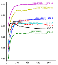
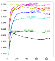
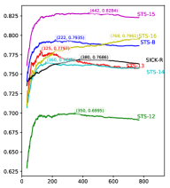
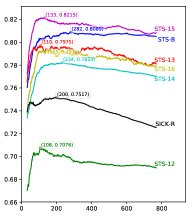
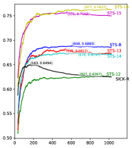
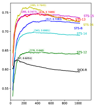
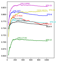
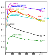
Dimensionality reduction is a crucial feature, because reduction of vector size brings about smaller memory occupation and a faster retrieval for downstream vector search engines. The dimensionality $k$ is a hyperparameter of reserved dimension of sentence embeddings, which can affect the model performance by large margin. Therefore, we carry out experiment to test the variation of Spearman’s correlation coefficient of the model with the change of dimensionality $k$. Figure 1 presents the variation curve of model performance under $\texttt{BERT}_{\texttt{base}}$ and $\texttt{BERT}_{\texttt{large}}$ embeddings. For most tasks, reducing the dimension of the sentence vector to its one of third is an relatively optimal solution, in which its performance is at the edge of increasing point.

In the SICK-R results in Table 1, although our $\texttt{BERT}_{\texttt{base}}\texttt{-whitening-256}\,(\texttt{NLI})$ is not as effective as $\texttt{BERT}_{\texttt{base}}\texttt{-flow}\,(\texttt{NLI})$, our model has a competitive advantage, i.e., the smaller embedding size (256 vs. 768). Furthermore, as presented in Figure 1(a), the correlation score of our $\texttt{BERT}_{\texttt{base}}\texttt{-whitening}\,(\texttt{NLI})$ raises to 66.52 when the embedding size is set to 109, which outperforms the $\texttt{BERT}_{\texttt{base}}\texttt{-flow}\,(\texttt{NLI})$ by 1.08 point. Besides, other tasks can also achieve better performances by choosing $k$ carefully.

5 Conclusion

In this work, we explore an alternative approach to alleviate the anisotropy problem of sentence embedding. Our approach is based on the whitening operation in machine learning, where experimental results indicate our method is simple but effective on 7 semantic similarity benchmark datasets. Besides, we also find that introduce dimensionality reduction operation can further boost the model performance, and naturally optimize the memory storage and accelerate the retrieval speed.

References

- Abdi and Williams (2010) Hervé Abdi and Lynne J Williams. 2010. Principal component analysis. Wiley interdisciplinary reviews: computational statistics, 2(4):433–459.
- Agirre et al. (2015) Eneko Agirre, Carmen Banea, Claire Cardie, Daniel Cer, Mona Diab, Aitor Gonzalez-Agirre, Weiwei Guo, Iñigo Lopez-Gazpio, Montse Maritxalar, Rada Mihalcea, German Rigau, Larraitz Uria, and Janyce Wiebe. 2015. SemEval-2015 task 2: Semantic textual similarity, English, Spanish and pilot on interpretability. In Proceedings of the 9th International Workshop on Semantic Evaluation (SemEval 2015), pages 252–263, Denver, Colorado. Association for Computational Linguistics.
- Agirre et al. (2014) Eneko Agirre, Carmen Banea, Claire Cardie, Daniel Cer, Mona Diab, Aitor Gonzalez-Agirre, Weiwei Guo, Rada Mihalcea, German Rigau, and Janyce Wiebe. 2014. SemEval-2014 task 10: Multilingual semantic textual similarity. In Proceedings of the 8th International Workshop on Semantic Evaluation (SemEval 2014), pages 81–91, Dublin, Ireland. Association for Computational Linguistics.
- Agirre et al. (2016) Eneko Agirre, Carmen Banea, Daniel Cer, Mona Diab, Aitor Gonzalez-Agirre, Rada Mihalcea, German Rigau, and Janyce Wiebe. 2016. SemEval-2016 task 1: Semantic textual similarity, monolingual and cross-lingual evaluation. In Proceedings of the 10th International Workshop on Semantic Evaluation (SemEval-2016), pages 497–511, San Diego, California. Association for Computational Linguistics.
- Agirre et al. (2012) Eneko Agirre, Daniel Cer, Mona Diab, and Aitor Gonzalez-Agirre. 2012. SemEval-2012 task 6: A pilot on semantic textual similarity. In *SEM 2012: The First Joint Conference on Lexical and Computational Semantics – Volume 1: Proceedings of the main conference and the shared task, and Volume 2: Proceedings of the Sixth International Workshop on Semantic Evaluation (SemEval 2012), pages 385–393, Montréal, Canada. Association for Computational Linguistics.
- Agirre et al. (2013) Eneko Agirre, Daniel Cer, Mona Diab, Aitor Gonzalez-Agirre, and Weiwei Guo. 2013. *SEM 2013 shared task: Semantic textual similarity. In Second Joint Conference on Lexical and Computational Semantics (*SEM), Volume 1: Proceedings of the Main Conference and the Shared Task: Semantic Textual Similarity, pages 32–43, Atlanta, Georgia, USA. Association for Computational Linguistics.
- Arora et al. (2017) Sanjeev Arora, Yingyu Liang, and Tengyu Ma. 2017. A simple but tough-to-beat baseline for sentence embeddings. In 5th International Conference on Learning Representations, ICLR 2017, Toulon, France, April 24-26, 2017, Conference Track Proceedings. OpenReview.net.
- Bowman et al. (2015) Samuel R. Bowman, Gabor Angeli, Christopher Potts, and Christopher D. Manning. 2015. A large annotated corpus for learning natural language inference. In Proceedings of the 2015 Conference on Empirical Methods in Natural Language Processing, pages 632–642, Lisbon, Portugal. Association for Computational Linguistics.
- Brown et al. (2020) Tom B. Brown, Benjamin Mann, Nick Ryder, Melanie Subbiah, Jared Kaplan, Prafulla Dhariwal, Arvind Neelakantan, Pranav Shyam, Girish Sastry, Amanda Askell, Sandhini Agarwal, Ariel Herbert-Voss, Gretchen Krueger, Tom Henighan, Rewon Child, Aditya Ramesh, Daniel M. Ziegler, Jeffrey Wu, Clemens Winter, Christopher Hesse, Mark Chen, Eric Sigler, Mateusz Litwin, Scott Gray, Benjamin Chess, Jack Clark, Christopher Berner, Sam McCandlish, Alec Radford, Ilya Sutskever, and Dario Amodei. 2020. Language models are few-shot learners. In Advances in Neural Information Processing Systems 33: Annual Conference on Neural Information Processing Systems 2020, NeurIPS 2020, December 6-12, 2020, virtual.
- Cer et al. (2017) Daniel Cer, Mona Diab, Eneko Agirre, Iñigo Lopez-Gazpio, and Lucia Specia. 2017. SemEval-2017 task 1: Semantic textual similarity multilingual and crosslingual focused evaluation. In Proceedings of the 11th International Workshop on Semantic Evaluation (SemEval-2017), pages 1–14, Vancouver, Canada. Association for Computational Linguistics.
- Cer et al. (2018) Daniel Cer, Yinfei Yang, Sheng-yi Kong, Nan Hua, Nicole Limtiaco, Rhomni St John, Noah Constant, Mario Guajardo-Céspedes, Steve Yuan, Chris Tar, et al. 2018. Universal sentence encoder. arXiv preprint arXiv:1803.11175.
- Christiansen (2010) Grant Christiansen. 2010. Data whitening and random tx mode. Texas Instruments.
- Conneau et al. (2017) Alexis Conneau, Douwe Kiela, Holger Schwenk, Loïc Barrault, and Antoine Bordes. 2017. Supervised learning of universal sentence representations from natural language inference data. In Proceedings of the 2017 Conference on Empirical Methods in Natural Language Processing, pages 670–680, Copenhagen, Denmark. Association for Computational Linguistics.
- Devlin et al. (2019) Jacob Devlin, Ming-Wei Chang, Kenton Lee, and Kristina Toutanova. 2019. BERT: Pre-training of deep bidirectional transformers for language understanding. In Proceedings of the 2019 Conference of the North American Chapter of the Association for Computational Linguistics: Human Language Technologies, Volume 1 (Long and Short Papers), pages 4171–4186, Minneapolis, Minnesota. Association for Computational Linguistics.
- Dinh et al. (2014) Laurent Dinh, David Krueger, and Yoshua Bengio. 2014. Nice: Non-linear independent components estimation. arXiv preprint arXiv:1410.8516.
- Ethayarajh (2019) Kawin Ethayarajh. 2019. How contextual are contextualized word representations? comparing the geometry of BERT, ELMo, and GPT-2 embeddings. In Proceedings of the 2019 Conference on Empirical Methods in Natural Language Processing and the 9th International Joint Conference on Natural Language Processing (EMNLP-IJCNLP), pages 55–65, Hong Kong, China. Association for Computational Linguistics.
- Gao et al. (2019) Jun Gao, Di He, Xu Tan, Tao Qin, Liwei Wang, and Tie-Yan Liu. 2019. Representation degeneration problem in training natural language generation models. In 7th International Conference on Learning Representations, ICLR 2019, New Orleans, LA, USA, May 6-9, 2019. OpenReview.net.
- Golub and Reinsch (1971) Gene H Golub and Christian Reinsch. 1971. Singular value decomposition and least squares solutions. In Linear algebra, pages 134–151. Springer.
- Humeau et al. (2019) Samuel Humeau, Kurt Shuster, Marie-Anne Lachaux, and Jason Weston. 2019. Real-time inference in multi-sentence tasks with deep pretrained transformers. arXiv preprint arXiv:1905.01969.
- Li et al. (2020) Bohan Li, Hao Zhou, Junxian He, Mingxuan Wang, Yiming Yang, and Lei Li. 2020. On the sentence embeddings from pre-trained language models. In Proceedings of the 2020 Conference on Empirical Methods in Natural Language Processing (EMNLP), pages 9119–9130, Online. Association for Computational Linguistics.
- Liu et al. (2019) Yinhan Liu, Myle Ott, Naman Goyal, Jingfei Du, Mandar Joshi, Danqi Chen, Omer Levy, Mike Lewis, Luke Zettlemoyer, and Veselin Stoyanov. 2019. Roberta: A robustly optimized bert pretraining approach. arXiv preprint arXiv:1907.11692.
- Marelli et al. (2014) Marco Marelli, Stefano Menini, Marco Baroni, Luisa Bentivogli, Raffaella Bernardi, and Roberto Zamparelli. 2014. A SICK cure for the evaluation of compositional distributional semantic models. In Proceedings of the Ninth International Conference on Language Resources and Evaluation (LREC’14), pages 216–223, Reykjavik, Iceland. European Language Resources Association (ELRA).
- Mu and Viswanath (2018) Jiaqi Mu and Pramod Viswanath. 2018. All-but-the-top: Simple and effective postprocessing for word representations. In 6th International Conference on Learning Representations, ICLR 2018, Vancouver, BC, Canada, April 30 - May 3, 2018, Conference Track Proceedings. OpenReview.net.
- Pennington et al. (2014) Jeffrey Pennington, Richard Socher, and Christopher Manning. 2014. GloVe: Global vectors for word representation. In Proceedings of the 2014 Conference on Empirical Methods in Natural Language Processing (EMNLP), pages 1532–1543, Doha, Qatar. Association for Computational Linguistics.
- Peters et al. (2018) Matthew Peters, Mark Neumann, Mohit Iyyer, Matt Gardner, Christopher Clark, Kenton Lee, and Luke Zettlemoyer. 2018. Deep contextualized word representations. In Proceedings of the 2018 Conference of the North American Chapter of the Association for Computational Linguistics: Human Language Technologies, Volume 1 (Long Papers), pages 2227–2237, New Orleans, Louisiana. Association for Computational Linguistics.
- Radford et al. (2019) Alec Radford, Jeffrey Wu, Rewon Child, David Luan, Dario Amodei, and Ilya Sutskever. 2019. Language models are unsupervised multitask learners. OpenAI blog, 1(8):9.
- Rahutomo et al. (2012) Faisal Rahutomo, Teruaki Kitasuka, and Masayoshi Aritsugi. 2012. Semantic cosine similarity. In The 7th International Student Conference on Advanced Science and Technology ICAST, volume 4, page 1.
- Reimers and Gurevych (2019) Nils Reimers and Iryna Gurevych. 2019. Sentence-BERT: Sentence embeddings using Siamese BERT-networks. In Proceedings of the 2019 Conference on Empirical Methods in Natural Language Processing and the 9th International Joint Conference on Natural Language Processing (EMNLP-IJCNLP), pages 3982–3992, Hong Kong, China. Association for Computational Linguistics.
- Williams et al. (2018) Adina Williams, Nikita Nangia, and Samuel Bowman. 2018. A broad-coverage challenge corpus for sentence understanding through inference. In Proceedings of the 2018 Conference of the North American Chapter of the Association for Computational Linguistics: Human Language Technologies, Volume 1 (Long Papers), pages 1112–1122, New Orleans, Louisiana. Association for Computational Linguistics.
- Yang et al. (2018) Yinfei Yang, Steve Yuan, Daniel Cer, Sheng-yi Kong, Noah Constant, Petr Pilar, Heming Ge, Yun-Hsuan Sung, Brian Strope, and Ray Kurzweil. 2018. Learning semantic textual similarity from conversations. In Proceedings of The Third Workshop on Representation Learning for NLP, pages 164–174, Melbourne, Australia. Association for Computational Linguistics.