Finite size effects and loss of self-averageness in the relaxational dynamics of the spherical Sherrington-Kirkpatrick model

Abstract

We revisit the gradient descent dynamics of the spherical Sherrington-Kirkpatrick ($p=2$) model with finite number of degrees of freedom. For fully random initial conditions we confirm that the relaxation takes place in three time regimes: a first algebraic one controlled by the decay of the eigenvalue distribution of the random exchange interaction matrix at its edge in the infinite size limit; a faster algebraic one determined by the distribution of the gap between the two extreme eigenvalues; and a final exponential one determined by the minimal gap sampled in the disorder average. We also analyse the finite size effects on the relaxation from initial states which are almost projected on the saddles of the potential energy landscape, and we show that for deviations scaling as $N^{-\nu}$ from perfect alignment the system escapes the initial configuration in a time-scale scaling as $\ln N$ after which the dynamics no longer “self-averages” with respect to the initial conditions. We prove these statements with a combination of analytic and numerical methods.

1 Introduction

Fully connected or large dimensional models with quenched random interactions are commonly used as mean-field models for physical systems. In addition, they are realistic models for problems in other branches of sciences. Examples are manifold and only some celebrated ones are neural networks [1], ecosystems [2] and macro-economy agent-based models [3]. In these areas, the number of degrees of freedom is large but much smaller than the Avogadro number, or the dimension of space is large but also finite. Therefore, the ideal physical thermodynamical limit is a long way from being attained. Finite size or finite dimensional fluctuations can be very important and in some cases completely dominate the dynamic behaviour.

While a rather complete understanding of the asymptotic dynamics of disordered mean-field like models in the strict thermodynamic limit has been achieved in the last decades [4, 5, 6], the knowledge of finite size fluctuations is not as developed. Having said so, after a few studies in the early 2000s [7, 8, 9, 10], there has been a resurgence of interest in the dynamics of finite size strongly interacting models with quenched randomness. These studies were boosted by the will to better grasp the relaxation of glassy systems. Most importantly, the goals were to distinguish the relaxation akin to gradient descent from activation over free-energy barriers and, especially, to quantify the role played by the latter in the approach to equilibrium [11, 12, 13, 14, 15, 16] (see also [17, 18, 19] from the mathematics literature).

In this paper we picked the simplest disordered model we know of, the so-called spherical $p=2$ or spherical Sherrington-Kirkpatrick model [20], and we studied its relaxation at zero temperature in instances with a finite numbers of degrees of freedom or modes. Around a decade ago, some studies focused on the finite size effects in equilibrium and the fluctuations induced by them [21, 22, 23], and many more recent mathematics papers also deal with these [24, 25, 26, 27, 28, 29, 30]. Here we concentrate on the relaxation dynamics and we build upon previous works performed in the strict thermodynamic limit [31, 32, 33, 34, 35, 36, 37] and for finite size systems [38]. Concretely,

• for high-$T$ initial conditions we revisit the fluctuations with respect to the random matrix realisation,

• for low-$T$ initial conditions - correlated with the random interaction matrix - we analyse the fluctuations with respect to the initial condition.

The paper is organised as follows. In Sec. 2 we introduce the model and we recall, very briefly, a few of its properties. Section 3 is devoted to the analysis of the fluctuations induced by the random matrix realisation after sub-critical quenches from random (flat) initial conditions. The next Sec. 4 treats the case of initial conditions correlated with the random matrix. Finally, in Sec. 5 we present our conclusions.

2 The model

The spherical Sherrington-Kirkpatrick or $p=2$ disordered system is a model of $N$ pair-wise interacting “spins” taking real values [20]. It is described by the Hamiltonian

$$H[\vec{S},z]=-\frac{1}{2}\sum_{i\neq j}J_{ij}s_{i}s_{j}+\frac{z}{2}\left(\sum_{i}s_{i}^{2}-N\right)=-\frac{1}{2}\vec{S}\cdot(\mathbf{J}\vec{S})+\frac{z}{2}\left(\vec{S}^{\,2}-N\right)\;.$$ (1)

In the last expression the spins have been arranged in an $N$ component vector $\vec{S}=(s_{1},\dots,s_{N})$. The coupling constants $J_{ij}$ are real and symmetric, and form a matrix in the Gaussian Orthogonal Ensemble (GOE), $\mathbf{J}=\{J_{ij}\}_{(i,j)\in[\![1,N]\!]\^{A}{{}^{2}}}$. They have mean and variance ${\rm I\!E}[J_{ij}]=0$ and ${\rm I\!E}[J_{ij}^{2}]=J^{2}/N$, the latter ensuring extensivity of the energy in the thermodynamic limit. The energy of the model is given by just the first term in eq. (1) and $z$ is a Lagrange multiplier enforcing the spherical constraint $|\vec{S}|^{2}=N$ which also reads

$$\vec{S}^{\,2}=\sum_{i}s_{i}^{2}=N\;.$$ (2)

Straightforwardly, the Hamiltonian is simplified when $\vec{S}$ is decomposed using the orthonormal eigen-basis $\{\vec{V}_{\mu}\}$, with $\vec{V}_{\mu}\cdot\vec{V}_{\nu}=\delta_{\mu\nu}$, of the coupling matrix $\mathbf{J}$. With the notation

$$s_{\mu}=\vec{S}\cdot\vec{V}_{\mu}$$ (3)

for the projections of $\vec{S}$ in these directions, the Hamiltonian becomes

$$H[\vec{S},z]=-\frac{1}{2}\sum_{\mu}(\lambda_{\mu}-z)s_{\mu}^{2}-\frac{z}{2}\,N\,,$$ (4)

where $\{\lambda_{\mu}\}_{\mu\in[\![1,N]\!]}$ are the set of eigenvalues of $\mathbf{J}$ (with associated eigenvectors $\{\vec{V}_{\mu}\}$) ordered such that $\lambda_{N}>\dots>\lambda_{1}$.

In the infinite $N$ limit, the eigenvalues of GOE matrices are distributed according to the Wigner semi-circle law of radius $2J$

$$\rho(\lambda)=\frac{1}{2\pi J^{2}}\sqrt{(2J)^{2}-\lambda^{2}}\qquad\qquad\mbox{for}\;\;\lambda\in[-2J,2J]$$ (5)

and zero otherwise [39]. At high temperatures, $T>J$, the equilibrium state is paramagnetic. At $T=J$ there is a second order phase transition towards a low-temperature phase with two equilibrium states related by spin inversion symmetry [20, 23], which makes this model closer to a disordered ferromagnet than to a true spin glass. Here and in what follows we set the Boltzmann constant to one.

In spite of the relative simplicity of its thermodynamic structure, the out of equilibrium dynamics show many complex features like slow relaxation and aging [31, 32, 33, 34, 35, 36, 37, 38]. The damped dynamics are governed by the set of Langevin equations:

$$\partial_{t}s_{i}(t)=\sum_{j(\neq i)}J_{ij}s_{j}(t)-z\big{(}t,\{s_{\mu}(0)\}\big{)}s_{i}(t)+\xi_{i}(t)\quad\qquad\forall i\in[\![1,N]\!]\;,$$ (6)

where $\xi_{i}(t)$ represents a Gaussian white noise with zero mean and variance $\langle\xi_{i}(t)\xi_{j}(t^{\prime})\rangle=2T\,\delta_{ij}\delta(t-t^{\prime})$, and $T$ is the temperature of a thermal bath. We absorbed the friction coefficient in the definition of time. Accordingly, the microscopic time-scale is in the new units equal to one. In the present work, we are interested in the deterministic limit of eqs. (6), which in the basis of eigenvectors read

$$\partial_{t}s_{\mu}(t)=\Big{[}\lambda_{\mu}-z\big{(}t,\{s_{\mu}(0)\}\big{)}\Big{]}s_{\mu}(t)\quad\qquad\forall\mu\in[\![1,N]\!]\;.$$ (7)

These dynamics can be considered to be the zero temperature limit of the Langevin equations (6). The initial conditions are $\{s_{\mu}(0)\}$ and in the expressions above we made explicit the fact that $z$ depends on time and on them as well.

In terms of thermodynamics the zero temperature free energy is directly its Hamiltonian $H[\vec{S},z]$. In the long-time limit the system must fall in a stable or metastable state of the free energy, and which of them should depend on the initial condition. By setting $\lim_{t\to\infty}\partial_{t}s_{\mu}(t)=0$ we obtain the criteria

$$\delta_{s_{\mu}}H[\vec{S},z]=-(\lambda_{\mu}-z)s_{\mu}=0\quad\qquad\forall\mu\in[\![1,N]\!]$$ (8)

and at all times, complemented by the spherical constraint in eq. (2). The solutions to this system of equations are

$$\vec{S}=\pm\sqrt{N}\,\vec{V}_{\mu}\qquad\qquad\mbox{and}\qquad\qquad z=\lambda_{\mu}\quad\qquad\forall\mu\in[\![1,N]\!]\;,$$ (9)

and they are $2N$ in number. Their stability is determined by the Hessian $\delta_{s_{\mu}}\delta_{s_{\nu}}H[\vec{S},z]=-\delta_{\mu,\nu}(\lambda_{\mu}-z)$. Taking a given metastable state $\vec{S}=\sqrt{N}\vec{V}_{\mu}$, the local landscape has $N-\mu$ stable directions, $\mu-1$ unstable directions and a marginal flat one. The energy of each of these configurations, or equivalently $H[\vec{S}=\sqrt{N}\vec{V}_{\mu},z=\lambda_{\mu}]$ is simply equal to $-\lambda_{\mu}N/2$. This energy landscape analysis predicts that the system should always equilibrate in one of the solutions $\pm\sqrt{N}\vec{V}_{N}$ as they are the only stable ones with respect to $H[\vec{S},z]$. The ground state energy density is then $e_{\rm eq}=-\lambda_{N}/2$. We recall that $\lambda_{N}=2J+J\zeta N^{-2/3}$ with $\zeta$ a random variable distributed by the Tracy-Widom form [40, 41]. Therefore, the equilibrium $z$ also depends on $N$ but we do not write it down explicitly to lighten the notation.

2.1 Sources of fluctuations

We are interested in the dynamic fluctuations induced by the finite system size. We consider two kinds of initial conditions, flat and projected (called staggered in [33]), that we define in Sec. 2.1.1. In the former case, the fluctuations are induced by the random matrix or, equivalently, by the set of eigenvalues $\{\lambda_{\mu}\}$, which vary close to the edge of $\rho(\lambda)$ in a way that we recall in Sec. 2.1.2. In the latter case, we focus on initial states that are strongly correlated with the random matrix, in the form of small deviations from perfect alignment with a metastable configuration $\vec{V}_{\alpha}$.

2.1.1 The initial conditions

The crucial point of the following study will be the choice of the initial condition $\vec{S}(0)=\{s_{\mu}(0)\}$. Generically, this vector can be written in the basis of eigenvectors of the $\mathbf{J}$ matrix as

$$\vec{S}(0)=\sum_{\nu}c_{\nu}\vec{V}_{\nu}\;,$$ (10)

with the normalization translating into the following condition on the coefficients $c_{\nu}$:

$$S^{2}(0)=\sum_{\nu\eta}c_{\nu}c_{\eta}\,\vec{V}_{\nu}\cdot\vec{V}_{\eta}=\sum_{\nu}c^{2}_{\nu}=N\;.$$ (11)

Interesting choices for the initial state are:

1. A flat distribution on the basis of eigenvectors, that is $c_{\nu}=1$ for all $\nu$, which can be associated to thermal equilibrium at a very high temperature. This choice was made in the main body of [33, 34], where the dynamics of the $N\to\infty$ system were considered, and in [38] where finite $N$ corrections were studied. It corresponds to

   $$s_{\mu}(0)=s^{\rm flat}_{\mu}(0)=1\quad\qquad\forall\mu\in[\![1,N]\!]\;.$$ (12)

2. A “projected” initial system $\vec{S}(0)$ is almost perfectly aligned with an eigenvector $\vec{V}_{\alpha}$, with just a small orthogonal random perturbation $\vec{\varepsilon}$. It can be implemented as follows:

   $$\vec{S}(0)=\vec{\varepsilon}+\sqrt{(N-\vec{\varepsilon}\cdot\vec{\varepsilon}\,)}\;\vec{V}_{\alpha}\quad\quad\text{with}\quad\quad\vec{\varepsilon}\cdot\vec{V}_{\alpha}=0\;\text{,}\quad\quad\text{and}\quad{\vec{\varepsilon}}^{\;2}\ll N\;.$$ (13)

   Therefore,

   $$s_{\mu(\neq\alpha)}(0)=s^{\rm proj}_{\mu(\neq\alpha)}(0)=\vec{\varepsilon}\cdot\vec{V}_{\mu}=\varepsilon_{\mu}\qquad\quad\mbox{and}\qquad\quad s_{\alpha}(0)=s^{\rm proj}_{\alpha}(0)=\sqrt{N-\varepsilon^{2}}\;.$$ (14)

   The normalisation of $\vec{S}(0)$ is ensured for all $\vec{\varepsilon}$. and ${\vec{\varepsilon}}^{\,2}\ll N$ implies $\sum_{\mu}\varepsilon_{\mu}^{2}\ll N$. The case $\vec{\varepsilon}=\vec{0}$, with $N\to\infty$ was also considered in [33]. Random fluctuations close to the projected initial states can then be generated by choosing random $\vec{\varepsilon}$ with the conditions above.

   We select in this paper a $\vec{\varepsilon}$ which yields the same projection of the initial condition on all the eigenvectors $\vec{V}_{\mu}$:

   $$\vec{\varepsilon}=X\sum_{\nu(\neq\alpha)}\vec{V}_{\nu}\qquad\implies\qquad\varepsilon_{\mu}=\vec{\varepsilon}\cdot\vec{V}_{\mu}=X\quad\forall\;\mu\neq\alpha\quad\mbox{and}\quad\varepsilon_{\alpha}=0\;,$$ (15)

   and

   $$s^{\rm proj}_{\mu(\neq\alpha)}(0)=X\qquad\mbox{and}\qquad s^{\rm proj}_{\alpha}(0)=\sqrt{N-X^{2}(N-1)}\approx\sqrt{N}\;.$$ (16)

   We then consider $X$ to be a Gaussian random variable with zero mean $\langle X\rangle_{i.c.}=0$ and $\langle X^{2}\rangle_{i.c.}=\varepsilon_{typ}^{2}\ll 1$, properties that ensure $\varepsilon^{2}\ll N$ since $\varepsilon^{2}=X^{2}\sum_{\mu(\neq\alpha)}1=X^{2}(N-1)\sim X^{2}N$. In the following we will always refer to this choice of initial conditions as the “projected initial conditions”.

Another relevant choice for $\vec{\varepsilon}$ would be to consider each component $\varepsilon_{\mu}$ as an i.i.d. Gaussian random variable with zero mean and variance $\varepsilon^{2}_{typ}$. However, the calculations are harder in this case and it was not worth pursuing them here.

2.1.2 The interaction matrix

The largest eigenvalue of a finite size $N\times N$ Gaussian Orthogonal Ensemble (GOE) matrix ${\mathbf{J}}$ scales as $\lambda_{N}=2J+J\zeta N^{-2/3}$ with $\zeta$ governed by the ($\beta=1$) Tracy-Widom distribution [40, 41].

The finite size corrections of the eigenvalue distribution function $\rho(\lambda)$ are especially important at its border, close to $\lambda_{N}$. The derivation of the exact finite size corrections at the edge of $\rho(\lambda)$ still remains open. In Refs. [39, 43] an asymptotic scaling function for $\lambda_{N}-\lambda=\mathcal{O}(N^{-2/3})$ has been derived and it reads

$$\rho_{edge}(\lambda)=\left\{\begin{array}[]{lll}aN^{1/3}(\lambda_{N}-\lambda)\;,&\quad N^{-2/3}(\lambda_{N}-\lambda)\rightarrow 0\;,\vspace{0.2cm}\\ \dfrac{1}{\pi}\sqrt{\lambda_{N}-\lambda}\;,&\quad N^{-2/3}(\lambda_{N}-\lambda)\rightarrow+\infty\;.\\ \end{array}\right.$$ (19)

The exact value of the coefficient $a$ is not known.

The level spacings $g_{\mu}$ are defined as $g_{\mu}=\lambda_{\mu}-\lambda_{\mu-1}$. The probability distribution of the first gap, $g_{N}\equiv\lambda_{N}-\lambda_{N-1}$, in the GOE was studied in [42, 43] and it scales as

$$\rho_{\rm gap}(g_{N},N)=N^{2/3}\ \rho_{\rm typ}(N^{2/3}g_{N})$$ (20)

where

$$\left\{\begin{array}[]{rcl}\rho_{\rm typ}(N^{2/3}g_{N})&\sim&b\,N^{2/3}g_{N}+o(N^{2/3}g_{N})\vspace{0.3cm}\\ \vspace{0.2cm}\ln{\rho_{\rm typ}(N^{2/3}g_{N})}&\sim&-\frac{2}{3}(N^{2/3}\,g_{N})^{3/2}+o(N\,g_{N}^{3/2})\end{array}\right.\qquad\mbox{for}\qquad\begin{array}[]{l}N^{2/3}g_{N}\rightarrow 0\;,\vspace{0.3cm}\\ \vspace{0.2cm}N^{2/3}g_{N}\rightarrow\infty\;,\end{array}$$ (21)

with $b$ another unknown constant.

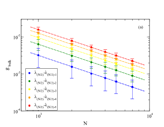
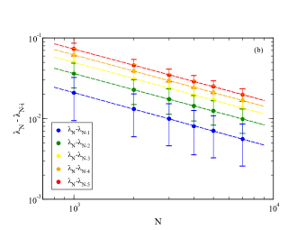
In Fig. 1 (a) we check a well-known result, the fact that $g_{\mu}=\lambda_{\mu}-\lambda_{\mu-1}$ in the bulk of the spectrum scales as $1/N$ [23]. In the same panel we display some other distances $\lambda_{\mu}-\lambda_{\mu-\nu}$ with $\nu=2,\dots,5$ and we verify that they all scale with $N$ in the same way. The data are averaged over ${\cal N}=1024$ samples of eigenvalues and the figure also shows the standard deviation. The $N$ dependence of the disorder averaged first gap as well as the one of other distances to the largest eigenvalue, $d_{i}=\lambda_{N}-\lambda_{i}$, are shown in Fig. 1 (b). Averages are also computed using ${\cal N}=1024$ samples of eigenvalues. All $d_{i}$ demonstrate an algebraic decay with $N$. In Table 1 we see that the fit exponent of the first gap, $g_{N}=d_{1}$, is slightly larger than the theoretically expected $2/3$, but also that the exponents seem to approach continuously the value $2/3$ for higher order distances.

Figure 1: (a) The $N$ dependence of the disorder averaged level spacing in the bulk. Check of the expected scaling $\lambda_{i}-\lambda_{i-1}\simeq N^{-1}$, on average and evaluation of the standard deviation. (b) The $N$ dependence of the disorder averaged distance to the largest eigenvalue, $d_{i}=\lambda_{N}-\lambda_{N-i}$ for $i=1\ldots 5$. The first gap, $g_{N}$, corresponds to $i=1$. Averages were taken over $1024$ sets of eigenvalues of the $\mathbf{J}$ matrix for each $N$. Details of the fits shown with dashed lines are shown in Table 1.

In the middle of the spectrum, the Wigner surmise predicts that the distribution of level spacings $g_{\mu}$ in the GOE ensemble takes the form of a Rayleigh distribution, with a linear increase from zero representing the level repulsion and a cross-over towards a Gaussian decay at large values of $g_{\mu}$:

$$\rho_{R}(x)=\frac{x}{\sigma^{2}}\,e^{-x^{2}/(2\sigma^{2})}$$ (22)

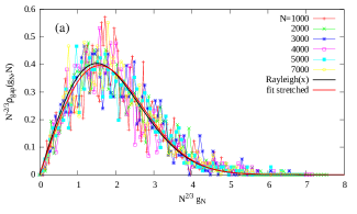
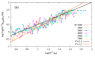
In Fig. 2 (a) we display the scaled probability distribution function of $g_{N}$ drawn from the same ensemble of ${\cal N}$ matrices, for the system sizes given in the key. The data are noisy and more samples would be needed to smooth it. The solid black curve is a Rayleigh distribution while the red one is a fit to the $N=7000$ data with a function of the form $f(x)=a\,x^{b}\exp{(-c\,x^{d})}$. The fit yields values of the exponents $b$ and $d$ which are very close to the Rayleigh ones. In panel (b) we zoom over the tail of the distribution and we present, in red, the line that corresponds to the fit with the exponent $d=2$ representing the Gaussian tail, and in black the stretched exponential tail with exponent $d=3/2$ predicted in [42, 43]. Within the uncertainty of the raw data, the figure shows that the latter gives a better representation of the data. Having said so, it is known that deriving the full distribution of $g_{N}$ is a very difficult task. For the GUE ensemble, this was achieved in [44] and a more manageable expression allowing for an asymptotic analysis was derived in [42, 43]. The techniques developed in [45] may allow one to obtain the gap distribution analytically in the GOE as well.

Figure 2: (a) Data collapse of the distribution of the first gap, $g_{N}$, for different system sizes according to eq. (20). In black a Rayleigh distribution and in red a fit to the $N=7000$ data (see text for details). (b) The distribution of the extreme $g_{N}$ values, with the Rayleigh Gaussian tail (in red) and the tail according to the Tracy-Widom behaviour [42] (in black).

Gap	$y=a\times x^{b}$		Standard Error
$\lambda_{N}-\lambda_{N-1}$	$a$	2,3315	0,03862183
	$b$	-0,6817	0,004794667
$\lambda_{N}-\lambda_{N-2}$	$a$	3,6211	0,02553595
	$b$	-0,66656	0,003170135
$\lambda_{N}-\lambda_{N-3}$	$a$	5,0813	0,02722184
	$b$	-0,66936	0,003379427
$\lambda_{N}-\lambda_{N-4}$	$a$	6,3192	0,02236387
	$b$	-0,66971	0,002776339
$\lambda_{N}-\lambda_{N-5}$	$a$	7,3988	0,02250885
	$b$	-0,66851	0,002794338

Table 1: Results of power law fits to the average distances from the largest eigenvalue shown in Fig. 1(b).

We are also interested in finding the minimum of the first gap, $g_{N}$, within the set of such gaps drawn from different random matrices labeled by $k=1,\dots,{\cal N}$:

$$g_{N}^{\rm min}({\cal N})=\min\limits_{k}g_{N}^{(k)}\;.$$ (23)

In the strict ${\cal N}\to\infty$ limit,

$$\lim_{{\cal N}\to\infty}g_{N}^{\rm min}({\cal N})=0\;,$$ (24)

given that $\rho_{\rm gap}$ has support on $g_{N}=[0,\infty)$. However, in typical samplings ${\cal N}$ is large but does not diverge and, therefore, $g_{N}^{\rm min}({\cal N})$ depends on ${\cal N}$. Indeed, it decreases with ${\cal N}$ in a way that we can estimate by assuming that there is typically one (or a few) value(s) $g_{N}^{(k)}$ in the interval $[0,\mu_{\cal N}]$, implying that [39]

$$\frac{1}{{\cal N}} = \int_{0}^{\mu_{\cal N}}dg_{N}\;\rho_{\rm gap}(g_{N})=\int_{0}^{\mu_{\cal N}}dg_{N}\;N^{2/3}\rho_{\rm typ}(N^{2/3}g_{N})=\int_{0}^{N^{2/3}\mu_{\cal N}}dy\;\rho_{\rm typ}(y)$$ (25)

$$\sim \int_{0}^{N^{2/3}\mu_{\cal N}}dy\;b\,y=\frac{b}{2}\;(N^{2/3}\mu_{\cal N})^{2}\qquad\implies\qquad\mu_{\cal N}\sim N^{-2/3}\;{\cal N}^{-1/2}\;.$$

In this way, we signalled out from the rest the minimal value we are looking for; it scales as

$$g_{N}^{\rm min}({\cal N})\sim N^{-2/3}\;{\cal N}^{-1/2}\;.$$ (26)

Figure 3: (a) The ${\mathcal{N}}$ dependence of the average minimal gap for random matrix sizes $N=1000-7000$ as indicated in the key. For each ${\mathcal{N}}$ an average over $1000$ random but correlated samples sorted from $1024$ uncorrelated ones was done. The dotted lines are fits to the data in the range $[2,64]$, where correlations are still not severe . (b) The same data as in panel (a) but showing the collapse expected according to equation (26) (see text for details). The dashed line is an interpolation with the expected power law.

$N$	$y=a\times x^{b}$		Standard Error
$1000$	$a$	0.020956	0.006281549
	$b$	-0.50896	0.01695654
$2000$	$a$	0.012077	0.005501834
	$b$	-0.46281	0,01485176
$3000$	$a$	0.0097188	0.005044484
	$b$	-0.48937	0.01361718
$4000$	$a$	0.0077346	0.006292685
	$b$	-0.48489	0.0169866
$5000$	$a$	0.0073124	0.005300066
	$b$	-0.53454	0.01430711
$7000$	$a$	0.0053732	0.007193261
	$b$	-0.48237	0.01941763

Table 2: Results of power law fits to the average minimal gaps shown in panel (a) of Fig. 3.

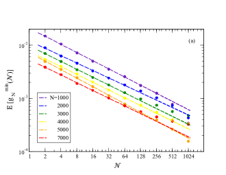
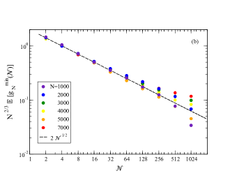
In Fig. 3 we show numerical results. A problem to obtain reliable numerical data on the minimal gaps is that a huge set of random matrices is needed. Note that a single $g_{N}^{\rm min}$ refers to the minimal value among a set of ${\cal N}$ random matrices, from each of which we extract the first gap $g_{N}$. In order to compute average values and fluctuations a large set of matrices needs to be diagonalized. For large matrix sizes $N$ this is a computationally demanding task. We decided to compute the average $g_{N}^{\rm min}$ for different matrix sizes by a resampling procedure. From an original set of $1024$ independent matrices we computed averages from $1000$ random sets of ${\cal N}$ matrices each. Of course, these sets are correlated. In panel (a) we see the results of the resampling procedure. For each system size $N$ the average $g_{N}^{\rm min}$ is shown together with a power law fit including the data for ${\cal N}\leq 64$. In Table 2 we show the results of the fits for each size. The fit exponents are not far from the expected value $1/2$. Furthermore, the prefactors should show a scaling with system size $N^{-2/3}$. In panel (b) of Fig. 3 we verify that sets with ${\cal N}\leq 64$ show a good data collapse in agreement with eq. (26). For larger set sizes deviations from the expected decay grow fast due to the strong correlations between sets for our limited number of independent samples.

2.2 The energy and the Lagrange multiplier

The fluctuating energy density,

$$e(t,N)=-\frac{1}{2N}\sum_{i\neq j}J_{ij}s_{i}(t)s_{j}(t)=-\frac{1}{2N}\sum_{\mu}\lambda_{\mu}s_{\mu}(t)s_{\mu}(t)\;,$$ (27)

is simply related to the fluctuating Lagrange multiplier $z$. This can be proven as follows. Multiplying the Langevin equation by $s_{\mu}(t^{\prime})$, summing over $\mu$, and taking $t^{\prime}\to t$ one has

$$\frac{1}{N}\sum_{\mu}(d_{t}s_{\mu}(t))s_{\mu}(t^{\prime}\to t)=2e(t,N)+z(t,N)\;.$$ (28)

In the left-hand-side we identify the time-derivative of the self-correlation

$$C(t,t^{\prime})=\frac{1}{N}\sum_{i}s_{i}(t)s_{i}(t^{\prime})=\frac{1}{N}\sum_{\mu}s_{\mu}(t)s_{\mu}(t^{\prime})$$ (29)

evaluated at equal times. Since it should vanish for all $N$ as a consequence of the normalisation $C(t,t)=1$, one then has

$$z(t,N)=-2e(t,N)$$ (30)

for any realisation of the random matrix and for all initial conditions.

An exact expression for $z$, and $e$, can next be deduced. The over-damped dynamic equation (7) is deterministic and its solution fixed by the initial condition. After a straightforward integration, the time-dependent spin configuration is given by

$$s_{\mu}(t)=s_{\mu}(0)\exp{\Big{[}\lambda_{\mu}t-\int_{0}^{t}dt^{\prime}\,z\big{(}t^{\prime},\{s_{\mu}(0)\}\big{)}\Big{]}}\,,$$ (31)

where we stressed that the Lagrange multiplier depends on the initial condition. In order to fix it, we impose the spherical constraint

$$N=\sum_{\mu}s^{2}_{\mu}(t)=\exp{\Big{[}-2\int_{0}^{t}dt^{\prime}\,z\big{(}t^{\prime},\{s_{\mu}(0)\}\big{)}\Big{]}}\sum_{\mu}s^{2}_{\mu}(0)\;e^{2\lambda_{\mu}t}$$

$$\qquad\qquad\implies\quad 2\int_{0}^{t}dt^{\prime}\,z\big{(}t^{\prime},\{s_{\mu}(0)\}\big{)}=\ln\Big{[}\frac{1}{N}\sum_{\mu}s^{2}_{\mu}(0)\;e^{2\lambda_{\mu}t}\Big{]}$$

$$\qquad\qquad\implies\quad z\big{(}t,\{s_{\mu}(0)\}\big{)}=\frac{\sum_{\mu}s^{2}_{\mu}(0)\;\lambda_{\mu}\;e^{2\lambda_{\mu}t}}{\sum_{\mu}s^{2}_{\mu}(0)\;e^{2\lambda_{\mu}t}}=\frac{1}{2}\frac{d}{dt}\ln\Big{[}\frac{1}{N}\sum_{\mu}s^{2}_{\mu}(0)\;e^{2\lambda_{\mu}t}\Big{]}\,.$$ (32)

Separating the contribution from the largest eigenvalue,

$$z\big{(}t,\{s_{\mu}(0)\}\big{)}=\lambda_{N}+\frac{1}{2}\frac{d}{dt}\ln{\mathcal{Z}}_{N}\big{(}t,\{s_{\mu}(0)\}\big{)}$$ (33)

with

$${\mathcal{Z}}_{N}\big{(}t,\{s_{\mu}(0)\}\big{)}=\frac{s^{2}_{N}(0)}{N}+\frac{1}{N}\sum_{\mu(\neq N)}s^{2}_{\mu}(0)\;e^{2(\lambda_{\mu}-\lambda_{N})t}$$ (34)

and ${\mathcal{Z}}_{N}\big{(}0,\{s_{\mu}(0)\}\big{)}=1$ for all initial conditions.

For finite size systems, any initial state that is not fully aligned with an eigenvector of the interaction matrix, and regardless of the scaling of time $t$ with $N$, the Lagrange multiplier converges to $\lambda_{N}$ when $t\rightarrow\infty$. Indeed, in the previous equation the two sums will eventually be dominated by the contribution of the largest eigenmode as long as the initial condition has some overlap with it. As an example

$$\sum_{\mu}s^{2}_{\mu}(0)\;e^{2\lambda_{\mu}t}\underset{t\rightarrow\infty}{=}s^{2}_{N}\;e^{2\lambda_{N}t}$$ (35)

and it follows that

$$z\big{(}t,\{s_{\mu}(0)\}\big{)} \underset{t\rightarrow\infty}{=} \Big{[}\lambda_{N}s_{N}^{2}(0)\;e^{2\lambda_{N}t}\Big{]}\Big{[}s^{2}_{N}(0)\;e^{2\lambda_{N}t}\Big{]}^{-1}=\lambda_{N}\;,\qquad\quad\forall\;\mbox{finite}\;N$$ (36)

and for all initial conditions with $s^{2}_{N}(0)\neq 0$.

Going back to eq. (33), this implies that the excess energy with respect to the ground state one is

$$\Delta e(t,N) = \lambda_{N}-e(t,N)$$ (37)

$$= \frac{1}{2}\;\frac{\sum\limits_{\mu(\neq N)}\;s_{\mu}^{2}(0)(\lambda_{N}-\lambda_{\mu})\;e^{2(\lambda_{\mu}-\lambda_{N})t}}{s_{N}^{2}(0)+\sum\limits_{\mu(\neq N)}s_{\mu}^{2}(0)e^{2(\lambda_{\mu}-\lambda_{N})t}}\;.$$

In the very last time-regime, assuming that only one term dominates the sums:

$$\Delta e(t,N)\to\frac{g_{N}s_{N-1}^{2}(0)}{2s_{N}^{2}(0)}\;e^{-2g_{N}t}\;,$$ (38)

with the gap between the last two eigenvalues defined as $g_{N}=\lambda_{N}-\lambda_{N-1}$. (The trivial case in which the initial configuration is correlated with the ground state and $s_{N}^{2}(0)$ scales with $N$ is excluded.)

The projection of the time-dependent spin vector $\vec{S}(t)$ on any of the eigenvectors $\vec{V}_{\mu}$, $s_{\mu}(t)=\vec{S}(t)\cdot\vec{V}_{\mu}$, reads

$$s_{\mu}(t)=s_{\mu}(0)\;\exp\left[\lambda_{\mu}t-\int_{0}^{t}dt^{\prime}\;z(t^{\prime},\{s_{\mu}(0)\})\right]=s_{\mu}(0)\;\exp\left[(\lambda_{\mu}-\lambda_{N})t+2\int_{0}^{t}dt^{\prime}\;\Delta e(t^{\prime},\{s_{\mu}(0)\})\right]\;.$$ (39)

3 Infinite temperature initial states

In this section we study the fluctuations with respect to the random matrix ${\mathbf{J}}$. The initial conditions are drawn from the flat distribution (i) defined in Sec. 2.1.1. The disorder averaged asymptotic ground state energy density of the infinite size system is expected to be equal to the one of any random couplings realization (self-averageness) and approach [33]

$$\lim_{t\gg 1}\lim_{N\to\infty}{\rm I\!E}[e(t,N)]=-1+\frac{3}{8t}\;,$$ (40)

where the first term in the r.h.s. is $-\lim_{N\to\infty}\lambda_{N}/2$ and henceforth we measure the energy in units of $J$.

For any $N$ and for fixed random interactions, from eqs. (30) and (36), $\lim_{t\to\infty}e(t,N)=-\lambda_{N}/2$. For $N$ large but finite Fyodorov et al. proved the existence of a cross-over time-scale $t_{\rm cross}={\mathcal{O}}(N^{2/3})$ between two regimes [38]. For $t\ll t_{\rm cross}$ the dynamics is well described by the one of the infinite size system. Instead, beyond this time scale, the system explores a sector of the potential energy landscape close to the ground state, and the relaxation is governed by a small number of saddle points with a number of unstable directions of ${\mathcal{O}}(1)$.

More precisely, in the finite $N$ system the mean excess energy density with respect to the ground state, ${\rm I\!E}[\Delta e(t,N)]={\rm I\!E}[e(t,N)+\lambda_{N}/2]$, behaves as

$${\rm I\!E}[\Delta e(t,N)]\sim\left\{\begin{array}[]{l}e_{1}(t)\\ N^{-2/3}\;f\left(tN^{-2/3}\right)\end{array}\right.\qquad\mbox{for}\qquad\begin{array}[]{l}t\ll N^{2/3}\\ t\geqslant N^{2/3}\end{array}$$ (41)

where the function $e_{1}(t)=3/(8t)$ makes contact with eq. (40), and $f(x)$ is a scaling function with the limits:

$$f(x)\sim\left\{\begin{array}[]{l}\dfrac{3}{8x}\vspace{0.2cm}\\ \dfrac{a}{x^{3}}\end{array}\right.\qquad\mbox{if}\qquad\begin{array}[]{l}x\to 0\vspace{0.5cm}\\ x\to\infty\end{array}$$ (42)

$a$ is an unknown constant. The regime $x\to 0$ corresponds to the thermodynamic limit, while $x\to\infty$ describes the late time behaviour of systems with large but finite $N$. Therefore, for $t>t_{\rm cross}$, the system escapes the self-averaging algebraic decay and enters another, faster and non self-averaging, but also algebraic decay. These features can be seen in Fig. 4.

Figure 4: Random matrix induced fluctuations of the excess energy in systems with $N=7000$ evolving from random initial conditions. Decay of the excess energy for systems with different realisations of the coupling strengths and, with a dashed black line, the average over 1024 such runs. Note the grouping of curves with different colour according to the deviation of the first gap $g_{N}$ from its average value (see the text for discussion).

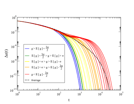
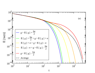
Figure 4 demonstrates the non self-averageness of the relaxation dynamics, at time-scales beyond $N^{2/3}$, in quenches from fully disordered initial conditions. The various curves represent the decay of the excess energy density in systems with size $N=7000$ for different realisations of the random matrix $\mathbf{J}$. After a self-averaging period that coincides with the regime in which the behaviour is the same as in the $N\to\infty$ limit, some instances start departing from the average, dominate it, and render the average algebraic though with a different power. In the figure, the different instances are grouped with different colours depending on the deviation of the first gap, $g_{N}$, from its average value. Note that the group where the gaps are the largest decay fast. Because of this fact these samples do not contribute to the second averaged algebraic regime (nor to the third and final regime). It can be further noticed that, at sufficiently long times, the average relaxation becomes still faster. In fact, this last decay towards the global minimum of the energy is exponential and ruled by the minimum gap, $g_{N}^{\rm min}$, as will be shown below.

Figure 5: Finite-size dependence of the disorder averaged excess energy with respect to the ground state, $\Delta e$, in systems evolving from random initial conditions. (a) Averages over 1024 disorder samples for different system sizes given in the key. (b) Scaling according to eqs. (41)-(42). In set I samples with $g_{N}>{\rm I\!E}(g_{N})-\sigma$ and in set II the samples with smaller gaps. The first two time regimes follow the analytic predictions in [33] and [38], respectively. The spreading of the curves at the longest times in set II is an indication of the breakdown of this scaling.

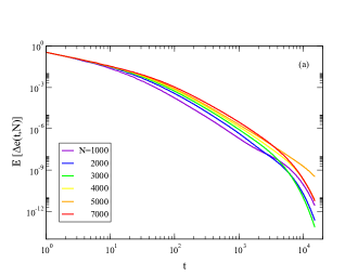
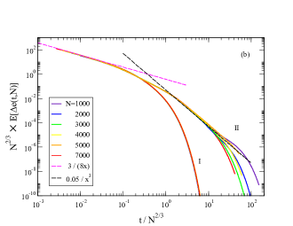
Figure 5 shows the decay of the disorder averaged excess energy for different system sizes. Each curve corresponds to an average over $1024$ samples of the matrix $\mathbf{J}$. The curves on the left panel are shown again in the right one after scaling according to eqs. (41)-(42) [38]. Similarly to what was done in Fig. 4, the averages were taken after dividing individual samples in two groups: in group I samples with $g_{N}>{\rm I\!E}(g_{N})-\sigma$ and in group II samples with smaller gaps. Clearly, the set with the smaller gaps is responsible for the second power law regime, while the larger gaps lead to fast, exponential decay. This set does not contribute to the averages in the second time scale. Power law fits, shown in dotted straight lines, are in good agreement with the theoretical predictions for the first two dynamical regimes, the one that coincides with the $N\to\infty$ results and the next algebraic one. The latter regime is governed by the statistical properties of the first gap $g_{N}=\lambda_{N}-\lambda_{N-1}$. From eq. (38) we obtain

$${\rm I\!E}[\Delta e(t,N)]\ \underset{t\rightarrow\infty}{\longrightarrow}\ {\rm I\!E}\left[\frac{g_{N}}{2}\;e^{-2g_{N}t}\right].$$ (43)

Using now the probability distribution of the first gap [43] recalled in eqs. (20)-(21), one can perform the average

$${\rm I\!E}[\Delta e(t,N)] = \int_{0}^{\infty}dr\;\frac{r}{2}\ e^{-2rt}\ \rho_{\rm gap}(r,N)$$ (44)

$$\sim \int_{0}^{N^{-2/3}}dr\;\frac{r}{2}e^{-2rt}\ bN^{4/3}r+\int_{N^{-2/3}}^{\infty}dr\;\frac{r}{2}e^{-2rt}\ N^{2/3}e^{-\frac{2}{3}(N^{2/3}r)^{3/2}}\$$

$$\sim \frac{b}{2}N^{4/3}t^{-3}\int_{0}^{t/N^{2/3}}dx\;x^{2}\ e^{-2x}+\frac{1}{2N^{2/3}}\int_{1}^{\infty}dx\ x\ e^{-2tN^{-2/3}x}\ e^{-\frac{2}{3}x^{3/2}}\;.$$

In the regime $t/N^{2/3}\gg 1$ the first term dominates, the second one is negligible, and the result can be re-arranged in the scaling form:

$${\rm I\!E}[\Delta e(t,N)] \sim \frac{b}{8N^{2/3}}\left(\frac{N^{2/3}}{t}\right)^{3}\;,$$ (45)

consistently with the fact that the average is dominated by the averaged contribution of the smaller gaps, that is to say, the regime $N^{2/3}g_{N}\to 0$ in eqs. (21). This is the second algebraic regime studied in [38].

Finally, we see a third and last time regime in which the averaged ${\rm I\!E}[\Delta e(t,N)]$ is controlled by the smallest gap found within the ensemble of random matrices used, $g_{N}^{\rm min}$. In this regime

$${\rm I\!E}[\Delta e(t,N)]\sim\frac{g_{N}^{\rm min}}{2}e^{-2g_{N}^{\rm min}t}\;.$$ (46)

Since we expect $g_{N}^{\rm min}\simeq{\cal N}^{-1/2}N^{-2/3}$, see eq. (26), the dependence on $N$ in the last regime is of the same form as the one in the second one, with $x=t/N^{2/3}$ the scaling variable.

Figure 6(a) illustrates this behaviour in the $N=7000$ case: the curves with different colours are averages over subsets of samples with the first gap in different ranges relative to the average gap. The curve on the extreme right, in red, is an average on the set of samples with the smaller gaps, $g<{\rm I\!E}(g)-3\sigma/2$, where $\sigma$ is the standard deviation of the first gap. The dotted black line corresponds to the average excess energy over the whole set of $1024$ samples. It approximates asymptotically to the rightmost curve, meaning that, as time grows, sets of samples with larger gaps gradually cease to contribute to the average.

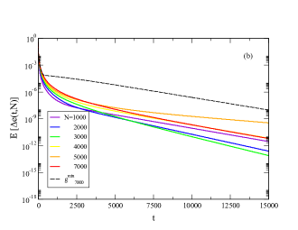
In Figure  6(b) the average excess energies for different system sizes are shown in log-linear scale, together with the data for the sample corresponding to the smallest gap, $g_{7000}^{min}$, for the $N=7000$ case (dotted black line). First of all, this scaling of the axes shows that at the longest times the decay approaches an exponential behaviour. The crossing of the curves for different system sizes reflects the large fluctuations in the value of the smallest gaps for each $N$. Finally, we note that the dotted line corresponding to the minimal gap for $N=7000$ goes, at the time scales shown, around three orders of magnitude above the curve for the average excess energy. This shows that, although at asymptotic long times there are a few exponentials contributing the the average excess energy, the approach to the longest time scale given by $1/g_{N}^{min}$ is approached very slowly. This is expected, given that the differences between the largest eigenvalue of the coupling matrix and the higher order neighbours scales similarly to the first gap, $\lambda_{N}-\lambda_{N-i}\propto N^{-2/3}$, as shown in Fig. 1(b) and Table 1.

Figure 6: The averaged excess energy illustrating the behaviour of the longest time regime. (a) Averages over subsets of samples grouped according to the distance of the first gap relative to the average for $N=7000$. (b) Averages for different sizes $N$ together with the decay of the sample with the minimal gap for $N=7000$.

Finally, the crossover time between the second and the third regime should be determined by

$$x^{-3}\sim{\cal N}^{-1/2}e^{-2{\cal N}^{-1/2}x}$$ (47)

with $x=t/N^{2/3}$. The solution increases (slowly) with increasing ${\cal N}$ and diverges, as expected, in the ${\cal N}\to\infty$ limit.

Summarizing the results for disordered initial conditions, we have seen that finite sized systems show three dynamical regimes. Two of them lead to algebraic relaxation. The first one is the trivial mean-field one, in which $N$ is so large that times can be considered finite with respect to it [33]. The second one was identified and described in [38]. We have firmly confirmed the theoretical expectations with numerical results for large system sizes. The last regime is exponential. We have shown that its scaling properties can be described exploiting the properties of the minimal gap drawn in the random matrix sampling, and hence depends on the size of the sampling matrix ensemble.

We can now examine the projection of the time-dependent spin vector on any of the eigenvectors, $s_{\mu}(t)=\vec{S}(t)\cdot\vec{V}_{\mu}$,

$$s_{\mu}(t)=s_{\mu}(0)\;\exp\left[(\lambda_{\mu}-\lambda_{N})t+2\int_{0}^{t}dt^{\prime}\;\Delta e(t^{\prime},\{s_{\mu}(0)\})\right]\;.$$ (48)

In the first regime we can exploit that the fluctuations of $\Delta e$ with respect to its expected value are negligible and then write

$$s_{\mu}(t)\simeq s_{\mu}(0)\;\exp\left[(\lambda_{\mu}-\lambda_{N})t+2\int^{t}dt^{\prime}\;\frac{3}{8t^{\prime}}\right]\simeq s_{\mu}(0)\;e^{(\lambda_{\mu}-\lambda_{N})t}\;t^{3/4}\;,$$ (49)

which at times of the order of the cross-over to the next regime $t\sim N^{2/3}$ becomes

$$s_{\mu}(t)\simeq s_{\mu}(0)\;e^{(\lambda_{\mu}-\lambda_{N})N^{2/3}}\;N^{1/2}\;.$$ (50)

It is clear that the modes which are at a larger distance than $N^{2/3}$ from the edge decay exponentially. Instead, those which are closer to $\lambda_{N}$ than $N^{2/3}$ grow with the system size. In particular, the projection on the last mode goes as $s_{N}(t)\simeq s_{\mu}(0)\;N^{1/2}$ by the end of this scale, and the mode has already gained a weight that scales with $N$ as in the equilibrium configuration. The rest of the evolution, in the second and third regimes, should then serve to make the weight identical to 1, as needed in the $T=0$ ground state.

We finally note that, as long as the initial conditions are of the flat kind, the fluctuations that they induce can be neglected and focus only on the fluctuations provoked by the random matrix, as we have done. We next turn to the study of the fluctuations induced by special initial conditions, which are near the stationary points of the potential energy landscape, the eigenvectors $\vec{V}_{\mu}$ of the random interaction matrix.

4 Initial states near metastable points

We now fix the random matrix ${\mathbf{J}}$ and we study the fluctuations with respect to initial conditions which are almost aligned with the eigenvectors of this matrix, the projected initial states (ii) defined in Sec. 2.1.1.

4.1 The escape time-scale

Starting with an initial condition of the form presented in eq. (13) we can identify a time scale after which the dynamics are no longer dominated by the direction of the initial state, i.e. $\vec{V}_{\alpha}$. In order to see this, in the equation that fixes $z\big{(}t,\{s_{\mu}(0)\}\big{)}$, eq. (32), we first separate the contribution of the $\alpha$ mode from the one of the rest of the eigenmodes:

$$z\big{(}t,\{s^{\rm proj}_{\mu}(0)\}\big{)} = \frac{\sum_{\mu(\neq\alpha)}\lambda_{\mu}\varepsilon^{2}_{\mu}\;e^{2\lambda_{\mu}t}+\lambda_{\alpha}(N-\vec{\varepsilon}\cdot\vec{\varepsilon}\,)\;e^{2\lambda_{\alpha}t}}{\sum_{\mu(\neq\alpha)}\varepsilon^{2}_{\mu}\;e^{2\lambda_{\mu}t}+(N-\vec{\varepsilon}\cdot\vec{\varepsilon}\,)\;e^{2\lambda_{\alpha}t}}\;.$$ (51)

Next we simplify the analysis by considering that all $\varepsilon_{\mu}$ are equal to a typical value called $\varepsilon_{typ}\ll 1$, see eq. (15), case (ii.a). In the large $N$ limit, $z\big{(}t,\{s^{\rm proj}_{\mu}(0)\}\big{)}$ boils down to

$$z\big{(}t,\{s^{\rm proj}_{\mu}(0)\}\big{)}=\dfrac{\varepsilon^{2}_{typ}\displaystyle{\int_{-2J}^{2J}}d\lambda\;\rho(\lambda)\lambda\;e^{2\lambda t}+\lambda_{\alpha}(1-\varepsilon_{typ}^{2})\;e^{2\lambda_{\alpha}t}}{\varepsilon^{2}_{typ}\displaystyle{\int_{-2J}^{2J}}d\lambda\;\rho(\lambda)\;e^{2\lambda t}+(1-\varepsilon_{typ}^{2})\;e^{2\lambda_{\alpha}t}}$$ (52)

which yields an exact expression when $\rho(\lambda)$ is the Wigner semi-circle law

$$z\big{(}t,\{s^{\rm proj}_{\mu}(0)\}\big{)}=\frac{\varepsilon^{2}_{typ}I_{2}(2\lambda_{N}t)/t+\lambda_{\alpha}(1-\varepsilon^{2}_{typ})\;e^{2\lambda_{\alpha}t}}{\varepsilon^{2}_{typ}I_{1}(2\lambda_{N}t)/(\lambda_{N}t)+(1-\varepsilon^{2}_{typ}\,)\;e^{2\lambda_{\alpha}t}}$$ (53)

with $I_{1}(y)$ and $I_{2}(y)$ modified Bessel functions. At the initial time $t\to 0$, we can use $\lim_{y\to 0}I_{a}(y)=(y/2)^{a}/\,\Gamma(a+1)$, and prove that

$$\lim_{t\to 0}z\big{(}t,\{s^{\rm proj}_{\mu}(0)\}\big{)}=\lambda_{\alpha}\left(1-\varepsilon^{2}_{typ}\right)\;,$$ (54)

while in the long time limit $\lambda_{N}t\gg 1$, $I_{a}(y)\to e^{y}/\sqrt{2\pi y}$, and

$$\lim\limits_{\lambda_{N}t\gg 1}z\big{(}t,\{s^{\rm proj}_{\mu}(0)\}\big{)}=\frac{\varepsilon_{typ}^{2}e^{2\lambda_{N}t}/(t\sqrt{4\pi\lambda_{N}t})+\lambda_{\alpha}(1-\varepsilon_{typ}^{2})e^{2\lambda_{\alpha}t}}{\varepsilon_{typ}^{2}e^{2\lambda_{N}t}/(\lambda_{N}t\sqrt{4\pi\lambda_{N}t})+(1-\varepsilon_{typ}^{2})e^{2\lambda_{\alpha}t}}\,.$$ (55)

If we assume that the first terms dominate the numerator and denominator, in the strict infinite time limit one recovers $\lim_{t\to\infty}z\big{(}t,\{s^{\rm proj}_{\mu}(0)\}\big{)}\to\lambda_{N}$. Otherwise, one can argue that the bulk weights as much as the mode $\alpha$ when the two contributions are roughly of the same order. Focusing on the ones in the numerator

$$\varepsilon^{2}_{typ}\;e^{2\lambda_{N}t}/\sqrt{4\pi\lambda_{N}t^{3}}\sim\lambda_{\alpha}(1-\varepsilon_{typ}^{2})\;e^{2\lambda_{\alpha}t}\;.$$ (56)

After some rearrangements and taking a $\ln$

$$-2(\lambda_{N}-\lambda_{\alpha})t\sim\ln\frac{\varepsilon^{2}_{typ}}{(1-\varepsilon_{typ}^{2})}-\frac{1}{2}\ln(4\pi)-\frac{1}{2}\ln(\lambda^{2}_{\alpha}\lambda_{N}t^{3})\;.$$ (57)

Assuming that the first term dominates the right-hand-side, in particular, that $\ln\varepsilon_{typ}\gg\ln(\lambda^{2}_{\alpha}\lambda_{N}t^{3})$, and $\lambda_{\alpha}\neq\lambda_{N}$,

$$t\sim-\frac{1}{\lambda_{N}-\lambda_{\alpha}}\,\ln\varepsilon_{typ}\equiv t_{\rm esc}\;,$$ (58)

where we defined a time-scale $t_{\rm esc}$. The same time scale would be identified from the analysis of the denominator in eq. (55). As a consequence, if $t$ is larger than the escape time scale outlined in eq. (58), the dynamics describe the departure of the system from its initial state $\vec{S}(0)\approx\sqrt{N}\vec{V}_{\alpha}$. We will see from the numerical solution of the dynamic equations, averaged over many such initial conditions, that this time scale characterises the cross over of $z\big{(}t,\{s^{\rm proj}_{\mu}(0)\}\big{)}$ from $\lambda_{\alpha}$ to $\lambda_{N}$. We point out that this analysis is naive in the sense that we have assumed that the bulk contribution can be replaced by an average over Wigner’s semi-circle law and the dependence on the initial conditions can be grasped from one typical realisation. Note that taking $\varepsilon_{typ}\sim N^{-\nu}$ the time-scale discussed above is

$$\varepsilon_{typ}\sim N^{-\nu}\qquad\quad\implies\qquad\quad t_{\rm esc}\sim\frac{\nu}{\lambda_{N}-\lambda_{\alpha}}\,\ln N$$ (59)

and, therefore, quite short. The escape from the initial condition occurs quickly, though in a time scale that grows with $N$.

4.2 Loss of self-averageness

In the previous Section we obtained a naive expression for $z$, eq. (53), that separates the contribution of the mode $\alpha$, along which the initial state is mostly aligned, from the one of the rest of the bulk. From it we identified the $N$-dependent escape time $t_{\rm esc}\sim\ln N$ for $\varepsilon_{\mu}=\varepsilon_{typ}=N^{-\nu}$ $\forall\mu$. In the following, we present an evaluation of $z$ where we carefully take the average over the projected initial conditions. It indicates that at this time-scale strong fluctuations with respect to the initial conditions appear.

4.2.1 The partition function point of view

As already mentioned in eq. (32), for all initial conditions and any $N$, the integral over time of the Lagrange multiplier reads

$$2\int_{0}^{t}dt^{\prime}\,z(t^{\prime},\{s_{\mu}(0)\})=\ln\Big{[}\frac{1}{N}\sum_{\mu}s^{2}_{\mu}(0)\,e^{2\lambda_{\mu}t}\Big{]}=\ln\Big{[}{\mathcal{Z}}_{N}\big{(}t,\{s_{\mu}(0)\}\big{)}\Big{]}\,.$$ (60)

The function ${\mathcal{Z}}_{N}\big{(}t,\{s_{\mu}(0)\}\big{)}$ can be interpreted as a partition function in the usual thermodynamics context. Here, the time $t$ plays the role of the inverse temperature $\beta$, $-2\lambda_{\mu}$ the role of the energy $E_{\mu}$, and $s^{2}_{\mu}(0)$ the role of a degeneracy $\Omega\big{(}E_{\mu}\big{)}$. Therefore, as time evolves the system is annealed in the sense of following lower and lower temperatures $T=1/\beta=1/t$. In the infinite time limit the system falls in the ground state corresponding to the lowest energy density $e_{\rm ground}=-\lim_{t\to\infty}z/2=-\lambda_{N}/2$. The correspondence with thermodynamics goes even further as the outlined partition function enables one to determine most of the relevant observables. As an example we have

$$z(t,\{s_{\mu}(0)\})=-2e[\vec{S}(t)]=\frac{1}{2}\frac{d}{dt}\ln\Big{[}{\mathcal{Z}}_{N}\big{(}t,\{s_{\mu}(0)\}\big{)}\Big{]}\;.$$ (61)

In the following we will determine the value taken by $z\big{(}t,\{s_{\mu}(0)\}\big{)}$ when the initial state $\vec{S}(0)$ is averaged out, indicated by the notation $\langle\dots\rangle_{i.c.}$. We will see that for projected initial conditions, beyond the time-scale $t_{\rm esc}$ the dynamics will not “self-average” with respect to the initial configurations.

To exactly evaluate $\langle\ln[{\mathcal{Z}}_{N}(t,\{s_{\mu}(0)\})]\rangle_{i.c.}$ we separate the contributions from the bulk and the $\alpha$ mode:

$$\ln\Big{[}{\mathcal{Z}}_{N}\big{(}t,\{s^{\rm proj}_{\mu}(0)\}\big{)}\Big{]}=\ln\Big{[}\frac{1}{N}\sum_{\mu}\ (s^{\rm proj}_{\mu}(0))^{2}\ e^{2\lambda_{\mu}t}\Big{]}=\ln\Big{[}\mathcal{Z}_{\rm bulk}\big{(}t,\{s^{\rm proj}_{\mu}(0)\}\big{)}+\frac{1}{N}(s^{\rm proj}_{\alpha}(0))^{2}\,e^{2\lambda_{\alpha}t}\Big{]}$$ (62)

with

$$\mathcal{Z}_{\rm bulk}\big{(}t,\{s^{\rm proj}_{\mu}(0)\}\big{)}=\frac{1}{N}\sum_{\mu(\neq\alpha)}(s^{{\rm proj}}_{\mu}(0))^{2}\ e^{2\lambda_{\mu}t}\;.$$ (63)

We recall that the projected initial conditions verify

$$s^{\rm proj}_{\mu(\neq\alpha)}(0)=X\qquad\mbox{and}\qquad s^{\rm proj}_{\alpha}(0)=\sqrt{N-X^{2}(N-1)}\approx\sqrt{N}$$ (64)

where $X$ is a Gaussian random variable with zero mean $\langle X\rangle_{i.c.}=0$ and $\langle X^{2}\rangle_{i.c.}=\varepsilon^{2}_{typ}\ll 1$, properties that ensure $\varepsilon^{2}\ll N$. We can thus rewrite the logarithm of the partition function as

$$\ln\Big{[}{\mathcal{Z}}_{N}\big{(}t,\{s^{\rm proj}_{\mu}(0)\}\big{)}\Big{]}=\ln\Big{[}\frac{X^{2}}{N}\sum_{\mu(\neq\alpha)}e^{2\lambda_{\mu}t}+e^{2\lambda_{\alpha}t}\Big{]}=\ln\Big{[}X^{2}\mathcal{Y}_{\rm bulk}(t)+e^{2\lambda_{\alpha}t}\Big{]}\;\;\;\;$$ (65)

with

$$\mathcal{Y}_{\rm bulk}(t)=\frac{1}{N}\sum_{\mu(\neq\alpha)}e^{2\lambda_{\mu}t}=\int d\lambda\,\rho(\lambda)\,e^{2\lambda t}=\frac{I_{1}(2\lambda_{N}t)}{\lambda_{N}t}\underset{t\to\infty}{\longrightarrow}\frac{e^{2\lambda_{N}t}}{\sqrt{4\pi}(\lambda_{N}t)^{3/2}}\;.$$ (66)

The next subsection detail how to study the fluctuations of $\ln\Big{[}{\mathcal{Z}}_{N}\big{(}t,\{s^{\rm proj}_{\mu}(0)\}\big{)}\Big{]}$ induced by these random initial conditions.

4.2.2 The distribution of ${\mathcal{Z}}_{N}\big{(}t,\{s^{\rm proj}_{\mu}(0)\}\big{)}$

The probability distribution $\rho\big{[}{\mathcal{Z}}_{N}\big{(}t,\{s^{\rm proj}_{\mu}(0)\}\big{)}\big{]}$, and its evolution with time, can be derived from the probability distribution of the initial configurations $\{s_{\mu}^{\rm proj}(0)\}$:

$$\rho\big{[}{\mathcal{Z}}_{N}\big{(}t,\{s^{\rm proj}_{\mu}(0)\}\big{)}\big{]} = \int\frac{dk}{2\pi}\frac{dX}{\sqrt{2\pi\varepsilon_{typ}^{2}}}\;\exp\Bigg{[}\frac{-X^{2}}{2\varepsilon_{typ}^{2}}+ik\Big{(}{\mathcal{Z}}_{N}\big{(}t,\{s^{\rm proj}_{\mu}(0)\}\big{)}-X\^{A}{{}^{2}}\mathcal{Y}_{\rm bulk}(t)-e^{2\lambda_{\alpha}t}\Big{)}\Bigg{]}\;,$$ (67)

where we used the Fourier representation of the Dirac delta. Integrating out the variable $X$ we obtain

$$\rho\big{[}{\mathcal{Z}}_{N}\big{(}t,\{s^{\rm proj}_{\mu}(0)\}\big{)}\big{]} = \int\frac{dk}{2\pi}\exp\Bigg{[}ik{\mathcal{Z}}_{N}\big{(}t,\{s^{\rm proj}_{\mu}(0)\}\big{)}-ike^{2\lambda_{\alpha}t}-\frac{1}{2}\ln\Big{(}1+2ik\varepsilon_{typ}^{2}\,\mathcal{Y}_{\rm bulk}(t)\Big{)}\Bigg{]}$$ (68)

$$\equiv \int\frac{dk}{2\pi}\exp\Big{[}S\big{(}k,{\mathcal{Z}}_{N}\big{(}t,\{s^{\rm proj}_{\mu}(0)\}\big{)}\Big{]}\;.$$

A first approach to simplify the action $S\big{(}k,{\mathcal{Z}}_{N}\big{(}t,\{s^{\rm proj}_{\mu}(0)\}\big{)}$ is to Taylor expand it around $k=0$:

$$\rho\big{[}{\mathcal{Z}}_{N}\big{(}t,\{s^{\rm proj}_{\mu}(0)\}\big{)}\big{]} = \int\frac{dk}{2\pi}\exp\Bigg{[}ik{\mathcal{Z}}_{N}\big{(}t,\{s^{\rm proj}_{\mu}(0)\}\big{)}-ike^{2\lambda_{\alpha}t}+\frac{1}{2}\sum_{m}\frac{\big{(}-2ik\varepsilon_{typ}^{2}\,\mathcal{Y}_{\rm bulk}(t)\big{)}^{m}}{m}\Bigg{]}\;$$ (69)

with the condition $2k\varepsilon_{typ}^{2}\,\mathcal{Y}_{\rm bulk}(t)<1$. By limiting the Taylor expansion to second order in $k$ it follows that

$$\rho\big{[}{\mathcal{Z}}_{N}\big{(}t,\{s^{\rm proj}_{\mu}(0)\}\big{)}\big{]} \sim \int\frac{dk}{2\pi}\exp\Bigg{[}ik{\mathcal{Z}}_{N}\big{(}t,\{s^{\rm proj}_{\mu}(0)\}\big{)}-ike^{2\lambda_{\alpha}t}-ik\varepsilon_{typ}^{2}\,\mathcal{Y}_{\rm bulk}(t)-k^{2}\varepsilon_{typ}^{4}\,\mathcal{Y}^{2}_{\rm bulk}(t)\Bigg{]}$$ (70)

$$\sim \frac{1}{\mathcal{N}^{\prime}}\exp\Bigg{[}\Big{(}{\mathcal{Z}}_{N}\big{(}t,\{s^{\rm proj}_{\mu}(0)\}\big{)}-e^{2\lambda_{\alpha}t}-\varepsilon_{typ}^{2}\,\mathcal{Y}_{\rm bulk}(t)\Big{)}^{2}/\Big{(}4\,\varepsilon_{typ}^{4}\,\mathcal{Y}^{2}_{\rm bulk}(t)\Big{)}\Bigg{]}$$

with $\mathcal{N}^{\prime}=\sqrt{4\pi\,\varepsilon_{typ}^{4}\,\mathcal{Y}^{2}_{\rm bulk}(t)}$. To this order, the distribution of ${\mathcal{Z}}_{N}\big{(}t,\{s^{\rm proj}_{\mu}(0)\}\big{)}$ is therefore Gaussian with mean

$$\Big{\langle}{\mathcal{Z}}_{N}\big{(}t,\{s^{\rm proj}_{\mu}(0)\}\big{)}\Big{\rangle}_{i.c.}=e^{2\lambda_{\alpha}t}+\varepsilon_{typ}^{2}\,\mathcal{Y}_{\rm bulk}(t)\underset{N\rightarrow\infty}{=}e^{2\lambda_{\alpha}t}+\varepsilon_{typ}^{2}\ \frac{I_{1}(2\lambda_{N}t)}{\lambda_{N}t}\underset{t\rightarrow\infty}{=}e^{2\lambda_{\alpha}t}+\frac{\varepsilon_{typ}^{2}}{(2\pi)^{1/2}}\ \frac{e^{2\lambda_{N}t}}{(\lambda_{N}t)^{3/2}}$$ (71)

and variance

$$\Big{\langle}\left({\mathcal{Z}}_{N}\big{(}t,\{s^{\rm proj}_{\mu}(0)\}\big{)}\!-\!\Big{\langle}{\mathcal{Z}}_{N}\big{(}t,\{s^{\rm proj}_{\mu}(0)\}\big{)}\Big{\rangle}_{i.c.}\right)^{2}\Big{\rangle}_{i.c.}\!\!\!\!\!\!\!=2\,\varepsilon_{typ}^{4}\,\mathcal{Y}^{2}_{\rm bulk}(t)\underset{N\rightarrow\infty}{\longrightarrow}2\,\varepsilon_{typ}^{4}\Big{(}\frac{I_{1}(2\lambda_{N}t)}{\lambda_{N}t}\Big{)}^{2}\!\!\!\underset{t\rightarrow\infty}{\longrightarrow}\!\frac{\varepsilon_{typ}^{4}}{\pi}\frac{e^{4\lambda_{N}t}}{(\lambda_{N}t)^{3}}\;.$$ (72)

As in Sec. 4.1, the characteristic time-scale $t_{\rm esc}$, see eq. (58), distinguishes two dynamic regimes in the large $N$ limit. When $t\ll t_{\rm esc}$, the standard deviation of the Gaussian distribution is negligible compared to its mean value. In this case the density distribution collapses to a delta function, i.e.

$$\rho\big{[}{\mathcal{Z}}_{N}\big{(}t,\{s^{\rm proj}_{\mu}(0)\}\big{)}\big{]}=\delta\Big{(}{\mathcal{Z}}_{N}\big{(}t,\{s^{\rm proj}_{\mu}(0)\}\big{)}-e^{2\lambda_{\alpha}t}-\varepsilon_{typ}^{2}\,\mathcal{Y}_{\rm bulk}(t)\Big{)}$$ (73)

and, straightforwardly, we recover the results of the previous Subsection. For instance,

$$2\Big{\langle}\int_{0}^{t}dt^{\prime}\,z(t^{\prime},\{s^{\rm proj}_{\mu}(0)\})\Big{\rangle}_{i.c.}=\Big{\langle}\ln\Big{[}{\mathcal{Z}}_{N}\big{(}t,\{s^{\rm proj}_{\mu}(0)\}\big{)}\Big{]}\Big{\rangle}_{i.c.}=\ln\Big{[}e^{2\lambda_{\alpha}t}+\varepsilon_{typ}^{2}\,\mathcal{Y}_{\rm bulk}(t)\Big{]}$$ (74)

and thus

$$\Big{\langle}z\big{(}t,\{s^{\rm proj}_{\mu}(0)\}\big{)}\Big{\rangle}_{i.c.}=\frac{\varepsilon^{2}_{typ}I_{2}(2\lambda_{N}t)/t+\lambda_{\alpha}\;e^{2\lambda_{\alpha}t}}{\varepsilon^{2}_{typ}I_{1}(2\lambda_{N}t)/(\lambda_{N}t)+\;e^{2\lambda_{\alpha}t}}\;,$$ (75)

which is identical to eq. (53).

However, when $t\gg t_{\rm esc}$, the mean and standard deviation of the Gaussian distribution scale evenly with the system size and the distribution does not simplify to a delta function. Besides, in this regime the truncation of the series in eq. (69) up to second order in $k$, and more generally the Taylor expansion of the logarithm, are no longer justified. Indeed, for a non-negligible part of the integral we verify $k\,\varepsilon_{typ}^{2}\,\mathcal{Y}_{bulk}(t)=\mathcal{O}(1)$, making all terms in the series count. The distribution of ${\mathcal{Z}}_{N}\big{(}t,\{s^{\rm proj}_{\mu}(0)\}\big{)}$ now exhibits fluctuations, meaning that the dynamics depend non-negligibly on its initial conditions.

In App. A we detail an alternative method to compute $\Big{\langle}\ln\Big{[}{\mathcal{Z}}_{N}\big{(}t,\{s^{\rm proj}_{\mu}(0)\}\big{)}\Big{]}\Big{\rangle}_{i.c.}$ in an exact manner, which has the benefit of also being more tractable numerically.

4.3 Numerical solution

To keep track of the fluctuations caused by the distribution of $\vec{\varepsilon}$, all our results are obtained with one fixed interaction matrix $\mathbf{J}$ with size $N\times N$ and averaged over 500 realizations of $\vec{\varepsilon}$. We used $\varepsilon_{typ}=N^{-1/2}$, i.e. $\nu=1/2$. In the following we represent the average over initial conditions with the notation $\langle\dots\rangle_{i.c.}$ and its standard deviation with $\Delta(\dots)$. As an example we consider

$$\Delta z\big{(}t,\{s_{\mu}(0)\}\big{)}=\langle z\^{A}{{}^{2}}\big{(}t,\{s_{\mu}(0)\}\big{)}\rangle_{i.c.}-\langle z\big{(}t,\{s_{\mu}(0)\}\big{)}\rangle\^{A}{{}^{2}}_{i.c.}\;.$$ (76)

The time scale $t_{\rm esc}$ in eq. (58) corresponds to the escape time from the initial state. For a system with $N=5000$ and $\lambda_{\alpha}=0$ it equals $t\sim 1/(2\lambda_{N})\ln N\simeq 2.13$. In Fig. 7(a) we observe the departure from the initial value, with the sudden shift of the Lagrange multiplier $z\big{(}t,\{s^{\rm proj}_{\mu}(0)\}\big{)}$, changing from $z=\lambda_{\alpha}=0J$ to a function converging to $\lambda_{N}=2J$. Numerically, we can identify a departure time $t_{\rm shift}$ as the time at which the function $z$ becomes concave,

$$\partial_{t}^{2}z\big{(}t,\{s_{\mu}(0)\}\big{)}\Big{|}_{t_{\rm shift}}=\;0\;.$$ (77)

Concretely, we calculate $t_{\rm shift}$ for each run and we then average over all of them to obtain $\langle t_{\rm shift}\rangle_{i.c.}$. $t_{\rm shift}$ is not necessarily equal to the time scale we identified with analytic arguments, $t_{\rm esc}$, but one can expect it to be of the same order of magnitude and to scale with $N$, and depend on other parameters, in a similar way. This is confirmed by the numerical results shown in Fig. 7(a). In eq. (58) we pointed out that the characteristic time-scale should scale with $N$ as ${\ln{N}}$, when we take $\varepsilon_{typ}\sim 1/\sqrt{N}$. Consequently, in Fig. 7(b) we plotted $t_{\rm shift}$ as function of $N$ and we obtained very good agreement with this prediction.

(a)                                                              (b)

Figure 7: (a) Time evolution of the Lagrange multiplier in a model with $N=5000$ with $\lambda_{\alpha}\sim 0$, and sampling data over 500 realisations of $\vec{\varepsilon}$ all with $z(0)\sim 0$ and randomness as in (ii). The black solid curve is the result of the microscopic dynamics averaged over initial conditions. The blue solid curve shows the fluctuations of $z$, $\Delta z$, as defined in eq. (76). The vertical dashed black line is the escape time (59) for $\lambda_{\alpha}=0$ and the horizontal one $z(t_{\rm esc})$ The vertical dashed orange line is the averaged value of $t_{\rm shift}$, the time when $z\big{(}t,\{s^{\rm proj}_{\mu}(0)\}\big{)}$ becomes convex. (b) Evolution of $t_{\rm shift}$ with the number of spins $N$. The dashed curves are guides-to-the-eye of the form $a_{\alpha}+b_{\alpha}\ln N$. Although it verifies $b_{\alpha}\propto\frac{1}{\lambda_{N}-\lambda_{\alpha}}$ the data deviate a bit from the other pre-factor $\nu$ expected from Eq. (59).

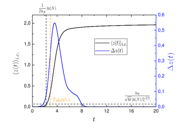
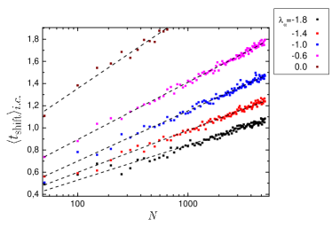
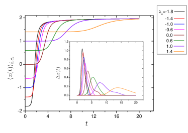
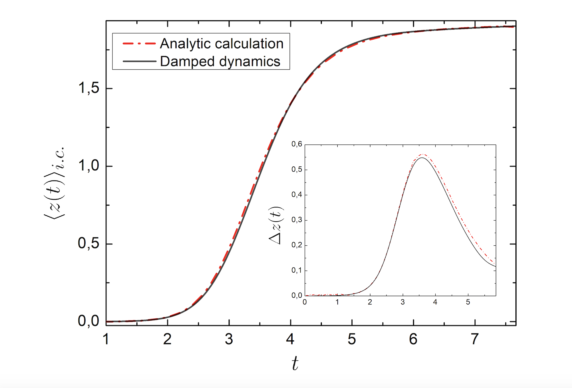
Figure 8 shows similar results for various initial states, $\vec{S}(0)=\vec{V}_{\alpha}+\vec{\varepsilon}$. In all cases the averaged Lagrange multiplier approaches the asymptotic value $\lambda_{N}$, but the pre-factor of time scales $t_{\rm esc}$ and $t_{\rm shift}$ depends on $\lambda_{\alpha}$. In the inset we display the fluctuations of $z$ for the same choices of initial conditions. Panel (b) in the same figure confronts the numerical results to the analytic predictions developed in App. A, from variations of eq. (81). The agreement is excellent for the averaged value and there are some tiny deviations for the fluctuations that diminish for increasing system size.

(a)                                                              (b)

Figure 8: (a) Time evolution of the averaged Lagrange multiplier after being averaged over projected initial conditions with different choices of $\vec{V}_{\alpha}$. In the inset, the fluctuations $\Delta z\big{(}t,\{s^{\rm proj}_{\mu}(0)\}\big{)}$ for the same parameters. (b) Comparison to the analytic predictions obtained with the free-energy $\langle\ln[{\mathcal{Z}}_{N}\big{(}t,\{s^{\rm proj}_{\mu}(0)\}\big{)}]\rangle_{i.c.}$ for $\lambda_{\alpha}=0$. In the main plot the average of $z$ and in the inset its fluctuatins. In both plots the system size is $N=5000$ and 500 realisations of the initial condition are used.

5 Discussion

In this paper we revisited the relaxation dynamics of the spherical Sherrington-Kirkpatrick or $p=2$ model. For infinite temperature initial conditions, we verified the predictions made in Refs. [33] and [38] for two algebraically decaying regimes of the excess energy density. In the first one, time is finite with respect to $N$, and the relaxation is controlled by the decay of $\rho(\lambda)$ at its edge in the $N\to\infty$ limit. The evolution crosses over to a second regime at a time-scale that depends on $N$ in a way determined by the distribution of the first gap, $\rho_{\rm gap}(g_{N})$. For GOE interaction matrices $t_{\rm cross}\sim N^{2/3}$. In terms of the time dependencies, e.g the excess energy relaxation in the second algebraic regime is faster than in the first one, $t^{-3}$ vs. $t^{-1}$. We employed much larger systems than previously used [38] and our numerical data fully confirm these predictions. We also identified the crossover to a last time regime in which the minimum first gap, $g^{\rm min}_{N}$, in a random matrix sampling of finite size, controls the average and is the inverse time-scale of the final exponential decay. For initial conditions mostly aligned with eigenvectors of the random exchange matrix, we found a time scale $t_{\rm esc}\sim t_{\rm shift}\sim\ln N$ beyond which the system departs considerably from the initial state and the dynamics lose their “self-averageness” with respect to the initial conditions. We proved this fact via a mapping to an effective partition function in which time plays the role of the inverse temperature. We calculated the corresponding free-energy with the replica method and from it we derived the average energy density and its fluctuations finding again excellent agreement with the numerical evaluation of the same quantities.

This model, albeit relatively simple since almost quadratic in nature, finds applications in many branches of physics and its interfaces. Some very recent examples are neural networks [46, 47], signal encryption [48], chaos in the classical limit of the Sachdev-Ye-Kitaev model [49], and integrability [50]. Fully understanding its behaviour for finite number of degrees of freedom will be of help in these areas as well.

Acknowldegements. We warmly thank G. Schehr for very helpful discussions. D.A.S aknowledges brazilian funding agency CNPq for partial financial support.

Appendix A Exact calculation of $\big{\langle}\ln[{\mathcal{Z}}_{N}\big{(}t,\{s^{\rm proj}_{\mu}(0)\}\big{)}]\,\big{\rangle}_{i.c.}$

We revisit the calculation of the average of ${\mathcal{Z}}_{N}$ over projected initial conditions. To exactly average over these initial states we apply the replica technique

$$\Big{\langle}\ln\Big{[}{\mathcal{Z}}_{N}\big{(}t,\{s^{\rm proj}_{\mu}(0)\}\big{)}\Big{]}\Big{\rangle}_{i.c.}\underset{n\rightarrow 0}{=}\frac{\Big{\langle}\Big{[}X\^{A}{{}^{2}}\mathcal{Y}_{\rm bulk}(t,\{J_{\mu}\})+e^{2\lambda_{\alpha}t}\Big{]}^{n}\Big{\rangle}_{i.c.}-1}{n}\;.$$ (78)

Focusing on the right-hand side of the previous equation we have

$$\Big{\langle}\Big{[}X\^{A}{{}^{2}}\,\mathcal{Y}_{\rm bulk}(t)+e^{2\lambda_{\alpha}t}\Big{]}^{n}\Big{\rangle}_{i.c.}=\sum_{n_{\alpha}=0}^{n}\ \binom{n}{n_{\alpha}}\ e^{2\lambda_{\alpha}n_{\alpha}t}\ \big{\langle}X^{2(n-n_{\alpha})}\big{\rangle}_{i.c.}\ \mathcal{Y}^{(n-n_{\alpha})}_{\rm bulk}(t)$$

$$\qquad\quad=\sum_{n_{\alpha}=0}^{n}\binom{n}{n_{\alpha}}\ e^{2\lambda_{\alpha}n_{\alpha}t}\ \frac{[2(n-n_{\alpha})]!}{(n-n_{\alpha})!\,2^{(n-n_{\alpha})}}\ \big{\langle}X^{2}\big{\rangle}^{n-n_{\alpha}}_{i.c.}\ \mathcal{Y}^{(n-n_{\alpha})}_{\rm bulk}(t)$$

$$\qquad\quad=\sum_{n_{\alpha}=0}^{n}\binom{n}{n_{\alpha}}\ e^{2\lambda_{\alpha}n_{\alpha}t}\ \binom{2n-2n_{\alpha}}{n-n_{\alpha}}(n-n_{\alpha})!\,\Bigg{(}\frac{\big{\langle}X^{2}\big{\rangle}_{i.c.}\ \mathcal{Y}_{\rm bulk}(t)}{2}\Bigg{)}^{(n-n_{\alpha})}$$

$$\qquad\quad=\sum_{n_{\alpha}=0}^{n}\ \frac{e^{2\lambda_{\alpha}n_{\alpha}t}}{4\pi\^{A}{{}^{2}}}\ \int_{-\pi}^{\pi}dx\int_{-\pi}^{\pi}dx^{\prime}\,\big{(}1+e^{ix}\big{)}^{n}e^{-ixn_{\alpha}}\big{(}1+e^{ix^{\prime}}\big{)}^{2(n-n_{\alpha})}e^{-ix^{\prime}(n-n_{\alpha})}$$

$$\qquad\quad\hskip 85.35826pt\times\ \int_{0}^{+\infty}dy\ e^{-y}\ y^{n-n_{\alpha}}\,\Bigg{(}\frac{\big{\langle}X^{2}\big{\rangle}_{i.c.}\mathcal{Y}_{\rm bulk}(t)}{2}\Bigg{)}^{(n-n_{\alpha})}$$

$$\qquad\quad=\frac{1}{4\pi^{2}}\int_{-\pi}^{\pi}dx\int_{-\pi}^{\pi}dx^{\prime}\int_{0}^{\infty}dy\ e^{-y}\ \Big{[}y\big{(}1+e^{ix}\big{)}\big{(}1+e^{ix^{\prime}}\big{)}^{2}e^{-ix^{\prime}}\Big{]}^{n}$$

$$\hskip 113.81102pt\times\ \Bigg{(}\frac{\big{\langle}X^{2}\big{\rangle}_{i.c.}\mathcal{Y}_{\rm bulk}(t)}{2}\Bigg{)}^{n}\times\ \sum_{n_{\alpha}=0}^{n}\Bigg{(}\frac{2\,e^{2\lambda_{\alpha}t+i(x^{\prime}-x)}}{y(1+e^{ix^{\prime}})^{2}\big{\langle}X^{2}\big{\rangle}_{i.c.}\ \mathcal{Y}_{\rm bulk}(t)}\Bigg{)}^{n_{\alpha}}\;.$$

Finally if we define the complex function

$$f(t,x,x^{\prime},y)=\frac{2\,e^{2\lambda_{\alpha}t+i(x^{\prime}-x)}}{y(1+e^{ix^{\prime}})^{2}\big{\langle}X^{2}\big{\rangle}_{i.c.}\mathcal{Y}_{\rm bulk}(t)}\;,$$ (79)

which contains the dependence on the initial condition through $\lambda_{\alpha}$, we obtain

$$\Big{\langle}\Big{[}X\^{A}{{}^{2}}\ \mathcal{Y}_{\rm bulk}(t)+e^{2\lambda_{\alpha}t}\Big{]}^{n}\Big{\rangle}_{i.c.} = \frac{1}{4\pi^{2}}\int_{-\pi}^{\pi}dx\int_{-\pi}^{\pi}dx^{\prime}\int_{0}^{+\infty}dy\,e^{-y}\ \Big{[}y\big{(}1+e^{ix}\big{)}\big{(}1+e^{ix^{\prime}}\big{)}^{2}e^{-ix^{\prime}}\Big{]}^{n}$$

$$\qquad\times\ \Bigg{(}\frac{\big{\langle}X^{2}\big{\rangle}_{i.c.}\mathcal{Y}_{\rm bulk}(t)}{2}\Bigg{)}^{n}\frac{1-f(t,x,x^{\prime},y)^{n+1}}{1-f(t,x,x^{\prime},y)}\;.$$

Taking the limit $n\rightarrow 0$ we determine the logarithm of the partition function, it yields

$$\Big{\langle}\ln\Big{[}{\mathcal{Z}}_{N}\big{(}t,\{s_{\mu}(0)\}\big{)}\Big{]}\Big{\rangle}_{i.c.} = \ln\Bigg{[}\frac{\big{\langle}X^{2}\big{\rangle}_{i.c.}\mathcal{Y}_{\rm bulk}(t)}{2}\Bigg{]}+\int_{0}^{+\infty}dy\,e^{-y}\ln y$$ (81)

$$-\frac{1}{4\pi^{2}}\int_{-\pi}^{\pi}dx\int_{-\pi}^{\pi}dx^{\prime}\int_{0}^{+\infty}dy\,e^{-y}\Bigg{[}\frac{f(t,x,x^{\prime},y)\ln[f(t,x,x^{\prime},y)]}{1-f(t,x,x^{\prime},y)}\Bigg{]}\;.$$

This expression demonstrates that $\langle\ln{\mathcal{Z}}_{N}\rangle_{i.c.}\neq\ln\langle{\mathcal{Z}}_{N}\rangle_{i.c.}$ and that there is no self-averageness with respect to the initial conditions. We will use it in the main text to evaluate the statistical properties of the Lagrange multiplier $z$ and hence of the energy density $e$.

We can readily check the two time limits $t\rightarrow 0$ and $t\rightarrow+\infty$. In the first one as we have $\langle X\^{A}{{}^{2}}\rangle_{i.c.}\ll 1$, the fraction in eq. (81) simplifies to

$$\frac{f(t,x,x^{\prime},y)\ln[f(t,x,x^{\prime},y)]}{1-f(t,x,x^{\prime},y)}\underset{t\rightarrow 0}{=}-\ln[f(t,x,x^{\prime},y)]$$ (82)

and we are left with

$$\Big{\langle}\ln\Big{[}{\mathcal{Z}}_{N}\big{(}t,\{s_{\mu}(0)\}\big{)}\Big{]}\Big{\rangle}_{i.c.} \underset{t\rightarrow 0}{=} \frac{1}{4\pi^{2}}\int_{-\pi}^{\pi}dx\int_{-\pi}^{\pi}dx^{\prime}\int_{0}^{+\infty}dy\,e^{-y}\;\ln\Bigg{[}\frac{e^{2\lambda_{\alpha}t+i(x^{\prime}-x)}}{(1+e^{ix^{\prime}})^{2}}\Bigg{]}$$ (83)

$$\underset{t\rightarrow 0}{=} 2\lambda_{\alpha}t\;.$$

This limit corresponds to the short-time dynamics where the system remains in its initial state. Indeed in this case we have $\vec{S}(t)\approx\sqrt{N}\vec{V}_{\alpha}$ and thus $z\big{(}t,\{s_{\mu}(0)\}\big{)}=\lambda_{\alpha}$.

In the case where $t\rightarrow+\infty$, all terms in eq. (81) are dominated by the highest eigenmode contribution. In other words the term $e^{2\lambda_{N}t}$ exponentially suppresses the function $f$:

$$\frac{f(t,x,x^{\prime},y)\ln[f(t,x,x^{\prime},y)]}{1-f(t,x,x^{\prime},y)} \underset{t\rightarrow+\infty}{=} f(t,x,x^{\prime},y)\ln[f(t,x,x^{\prime},y)]$$ (84)

$$\underset{t\rightarrow+\infty}{=} 0\;.$$

It then follows that

$$\Big{\langle}\ln\Big{[}{\mathcal{Z}}_{N}\big{(}t,\{s_{\mu}(0)\}\big{)}\Big{]}\Big{\rangle}_{i.c.} \underset{t\rightarrow+\infty}{=} \ln\Bigg{[}\frac{\big{\langle}X^{2}\big{\rangle}_{i.c.}\mathcal{Y}_{\rm bulk}(t)}{2}\Bigg{]}+\int_{0}^{+\infty}dy\,e^{-y}\ln y$$ (85)

$$\underset{t\rightarrow+\infty}{=} 2\lambda_{N}t\,.$$

Here the system has fallen in the lowest eigenmode, the only stable one.

References

- [1] J. J. Hopfield, Neural networks and physical systems with emergent collective computational abilities, Proc. Nat. Acad. Sc. 79, 2554 (1982).
- [2] R. May, Qualitative Stability in Model Ecosystems, Ecology, 54 638 (1972).
- [3] S. Gualdi, M. Tarzia, F. Zamponi, and J. P. Bouchaud, Tipping points in macro-economic agent-based models, Journal of Economic Dynamics and Control 50, 29 (2015).
- [4] L. F. Cugliandolo, Dynamics of glassy systems in Slow Relaxations and nonequilibrium dynamics in condensed matter, ed. by J.-L. Barrat et al., Les Houches Session LXXVII (Springer-Verlag, Berlin, 2003).
- [5] L. Berthier and G. Biroli, Theoretical perspective on the glass transition and amorphous materials, Rev. Mod. Phys. 83, 587 (2011).
- [6] F. Zamponi, Mean field theory of spin glasses, Lecture notes, arXiv:1008.4844
- [7] A. Crisanti and F. Ritort, Activated processes and inherent structure dynamics of finite-size mean-field models for glasses, Europhys. Lett. 52, 640 (2000).
- [8] A. Crisanti and F. Ritort, Potential energy landscape of finite-size mean-field models for glasses, Europhys. Lett. 51, 147 (2000).
- [9] A. Crisanti and F. Ritort, Intermittency of glassy relaxation and the emergence of a non-equilibrium spontaneous measure in the aging regime Europhys. Lett. 66, 253 (2004).
- [10] A. Billoire, L. Giomi, and E. Marinari, The mean-field infinite range p = 3 spin glass: Equilibrium landscape and correlation time scales, Europhys. Lett. 71, 824 (2005).
- [11] M. Baity-Jesi, G. Biroli, G. and C. Cammarota, Activated aging dynamics and effective trap model description in the random energy model, J. Stat. Mech. 2018 013301 (2018).
- [12] M. Baity-Jesi, A. Achard-de Lustrac and G. Biroli, Activated dynamics: An intermediate model between the random energy model and the p-spin model, Phys. Rev. E 98, 012133 (2018).
- [13] D. A. Stariolo and L. F. Cugliandolo, Activated dynamics of the Ising p-spin disordered model with finite number of variables, EPL 127, 16002 (2019).
- [14] D. A. Stariolo and L. F. Cugliandolo, Barriers, trapping times and overlaps between local minima in the dynamics of the disordered Ising p-spin Model, Phys. Rev. E 102, 022126 (2020).
- [15] V. Ros, C. Cammarota, and G. Biroli, Dynamical instantons and activated processes in mean-field glass models, SciPost Physics 10, 002 (2021).
- [16] M. Baity-Jesi, G. Biroli, and D. R. Reichman, Revisiting the Concept of Activation in Supercooled Liquids, arXiv:2103.07211.
- [17] G. Ben Arous and A. Jagannath, Spectral gap estimates in mean field spin glasses, Comm. Math. Phys. 361, 1 (2018).
- [18] A. Jagannath, Dynamics of mean field spin glasses on short and long timescales, J. Math. Phys. 60, 083305 (2019)
- [19] A. Dembo and R. Gheissari, Diffusions interacting through a random matrix: universality via stochastic Taylor expansion, arXiv:2006.13167, Probab. Th. and Relat. Fields (2021).
- [20] J. M. Kosterlitz, D. J. Thouless, and R. C. Jones, Spherical Model of a Spin-Glass, Phys. Rev. Lett 36, 1217 (1976).
- [21] L. F. Cugliandolo, D. S. Dean, and H. Yoshino, Nonlinear susceptibilities of spherical models, J. Phys. A 40, 4285 (2007).
- [22] C. Monthus and T. Garel, Typical versus averaged overlap distribution in Spin-Glasses: Evidence for the droplet scaling theory, Phys. Rev. B 88, 134204 (2013).
- [23] Y. V. Fyodorov and P. Le Doussal, Topology trivialization and large deviations for the minimum in the simplest random optimization, J. Stat. Phys. 154, 466 (2014).
- [24] J. Baik and J. O. Lee, Fluctuations of the free energy of the spherical Sherrington-Kirkpatrick model, J. Stat. Phys. 165 185 (2016).
- [25] J. Baik, J. O. Lee, and H. Wu, Ferromagnetic to paramagnetic transition in spherical spin glass, J. Stat. Phys. 173 1484 (2018).
- [26] P. Kivimae, Critical fluctuations for the spherical Sherrington-Kirkpatrick model in an external field, arXiv:1908.07512.
- [27] V. L. Nguyen and P. Sosoe, Central limit theorem near the critical temperature for the overlap in the 2-spin spherical SK model, J. Math. Phys. 60 103302 (2019).
- [28] B. Landon and P. Sosoe, Fluctuations of the overlap at low temperature in the 2-spin spherical SK model, arXiv:1905.03317.
- [29] B. Landon and P. Sosoe, Fluctuations of the 2-spin SSK model with magnetic field, arXiv:2009.12514.
- [30] J. Baik, E. Collins-Wildman, P. Le Doussal, and H. Wu, Spherical spin glass model with external field, arXiv:2010.06123.
- [31] P. Shukla and S. Singh, Spin glass dynamics in the spherical model, J. Phys. C 14, L81 (1981).
- [32] S. Ciuchi and F. di Pasquale, Nonlinear relaxation and ergodicity breakdown in random anisotropy spin glasses, Nucl. Phys. B [FS] 300, 31 (1988).
- [33] L. F. Cugliandolo and D. S. Dean, Full dynamic solution for a spherical spin-glass model, J. Phys. A: Math. Gen. 28, 4213 (1995).
- [34] L. F. Cugliandolo and D. S. Dean, On the dynamics of the spherical spin-glass in a magnetic field, J. Phys. A: Math. Gen. 28, L453 (1995).
- [35] G. Ben Arous, A. Dembo, and A. Guionnet, Aging of spherical spin-glass, Probab. Th. Relat. Fields 120, 1 (2001).
- [36] C. Chamon, L. F. Cugliandolo, and H. Yoshino, Fluctuations in the coarsening dynamics of the O(N) model: are they similar or different to those in glassy systems?, J. Stat. Mech (2006) P01006.
- [37] K. van Duijvendijk, R. L. Jack, and F. van Wijland, Second-order dynamic transition in a p=2 spin-glass model, Phys. Rev. E 81, 011110 (2010).
- [38] Y. V. Fyodorov, A. Perret, and G. Schehr, Large time zero temperature dynamics of the spherical p=2 spin glass model of finite size, J. Stat. Mech. 2015 P11017 (2015).
- [39] M. L. Mehta, Random Matrices, 2nd Edition (Academic Press, New York, 1991).
- [40] C. A. Tracy and H. Widom, Level-spacing distributions and the Airy kernel, Comm. Math. Phys. 159, 151 (1994).
- [41] C. A. Tracy and H. Widom, On orthogonal and symplectic matrix ensembles, Comm. Math. Phys. 177, 727 (1996).
- [42] A. Perret and G. Schehr, Near-extreme eigenvalues and the first gap of Hermitian random matrices, J. Stat. 156, 843 (2014).
- [43] A. Perret and G. Schehr, The density of eigenvalues seen from the soft edge of random matrices in the Gaussian beta-ensembles, Acta Phys. Pol. B 46, 1693 (2015).
- [44] N. S. Witte, F. Bornemann and P. J. Forrester, Joint distribution of the first and second eigenvalues at the soft edge of unitary ensembles, Nonlinearity 26, 1799 (2013).
- [45] A. Mays, A. Ponsaing and G. Schehr, Tracy-Widom distributions for the Gaussian orthogonal and symplectic ensembles revisited: a skew-orthogonal polynomials approach, J. Stat. Phys. 182, 28 (2021).
- [46] D. Marti, N. Brunel, and S. Ostojic, Correlations between synapses in pairs of neurons slow down dynamics in randomly connected neural networks, Phys. Rev. E 97, 062314 (2018).
- [47] S. Franz, A. Sclocchi, and P. Urbani Critical jammed phase of the linear perceptron, Phys. Rev. Lett. 123, 115702 (2019),
- [48] Y. V. Fyodorov, A Spin Glass Model for Reconstructing Nonlinearly Encrypted Signals Corrupted by Noise, J. Stat. Phys. 175, 789 (2019).
- [49] T. Scaffidi and E. Altman, Chaos in a classical limit of the Sachdev-Ye-Kitaev model, Phys. Rev. B 100, 155128 (2019).
- [50] D. Barbier, L. F. Cugliandolo, G. S. Lozano, and N. Nessi, (Non-equilibrium) thermodynamics of integrable models: The Generalized Gibbs Ensemble description of the classical Neumann model, EPL 132, 50002 (2020).