$W^{+}W^{-}$ production at NNLO+PS with MINNLO${}_{\text{PS}}$

Abstract

We consider $W^{+}W^{-}$ production in hadronic collisions and present the computation of next-to-next-to-leading order accurate predictions consistently matched to parton showers (NNLO+PS) using the MiNNLO_PS method. Spin correlations, interferences and off-shell effects are included by calculating the full process $pp\to e^{+}\nu_{e}\mu^{-}\bar{\nu}_{\mu}$. This is the first NNLO+PS calculation for $W^{+}W^{-}$ production that does not require an a-posteriori multi-differential reweighting. The evaluation time of the two-loop contribution has been reduced by more than one order of magnitude through a four-dimensional cubic spline interpolation. We find good agreement with the inclusive and fiducial cross sections measured by ATLAS and CMS. Both NNLO corrections and matching to parton showers are important for an accurate simulation of the $W^{+}W^{-}$ signal, and their matching provides the best description of fully exclusive $W^{+}W^{-}$ events to date.

1 Introduction

Precision phenomenology has evolved to one of the cornerstones of todays physics programme at the Large Hadron Collider (LHC). Without clear hints for new physics, the precise measurement of production rates and distributions of Standard Model (SM) processes provides a valuable path towards the observation of deviations from the SM picture. The production of vector-boson pairs is among the most important LHC signatures in that respect. Those processes are crucial to constrain or measure anomalous interactions among SM particles, such as anomalous couplings among three vector bosons (triple-gauge couplings), as any small deviation from the expected rates or shapes of distributions could be a signal of new physics.

$W^{+}W^{-}$ production has the largest cross section among the massive diboson processes and it provides direct access to triple-gauge couplings, which appear already in the leading perturbative contribution to the cross section. The measurement of this process at the LHC is a direct probe of the gauge symmetry structure of electroweak (EW) interactions and of the mechanism of EW symmetry breaking in the SM. Moreover, $W^{+}W^{-}$ final states are an irreducible background to Higgs measurements in the $H\to W^{+}W^{-}$ decay channel and to direct searches for BSM particles decaying into two leptons, missing energy, and/or jets. The $W^{+}W^{-}$ cross section has been measured at both the Tevatron Aaltonen:2009aa ; Abazov:2009ys ; Abazov:2011cb and the LHC (at 7 TeV Aad:2012oea ; ATLAS:2012mec ; Chatrchyan:2013yaa ; Aad:2014mda , 8 TeV Aad:2016wpd ; Chatrchyan:2013oev ; Khachatryan:2015sga ; Aaboud:2017cgf and 13 TeV Aaboud:2019nkz ; Aaboud:2017qkn ; CMS:2016vww ; Sirunyan:2020jtq ). The high sensitivity to anomalous triple-gauge couplings has been exploited in various indirect BSM searches Abazov:2009ys ; Aaltonen:2009aa ; ATLAS:2012mec ; Aad:2012oea ; Chatrchyan:2013yaa ; Chatrchyan:2013fya ; Aad:2014mda ; CMS:2015uda ; Khachatryan:2015sga ; Aad:2016wpd ; Aaboud:2017cgf ; Sirunyan:2017bey ; Aad:2021dse and the irreducible $W^{+}W^{-}$ background has been extensively studied in the context of $H\to W^{+}W^{-}$ decays in refs. Binoth:2005ua ; Campbell:2011cu ; Aad:2012me ; Aad:2013wqa ; Chatrchyan:2013iaa ; Campbell:2013wga ; ATLAS:2014aga ; Khachatryan:2014kca ; Aad:2015xua ; Aad:2015rwa ; Aad:2015ona ; Aad:2016lvc ; Caola:2016trd .

The theoretical description of fiducial cross sections and kinematic distributions has been greatly improved by the calculation of next-to-next-to-leading order (NNLO) corrections in QCD perturbation theory, which have become the standard for $2\to 1$ and $2\to 2$ colour-singlet production Ferrera:2011bk ; Ferrera:2014lca ; Ferrera:2017zex ; Campbell:2016jau ; Harlander:2003ai ; Harlander:2010cz ; Harlander:2011fx ; Buehler:2012cu ; Marzani:2008az ; Harlander:2009mq ; Harlander:2009my ; Pak:2009dg ; Neumann:2014nha ; deFlorian:2013jea ; deFlorian:2016uhr ; Grazzini:2018bsd ; Catani:2011qz ; Campbell:2016yrh ; Grazzini:2013bna ; Grazzini:2015nwa ; Campbell:2017aul ; Gehrmann:2020oec ; Cascioli:2014yka ; Grazzini:2015hta ; Heinrich:2017bvg ; Kallweit:2018nyv ; Gehrmann:2014fva ; Grazzini:2016ctr ; Grazzini:2016swo ; Grazzini:2017ckn ; Baglio:2012np ; Li:2016nrr ; deFlorian:2019app . With $\gamma\gamma\gamma$ production even the first $2\to 3$ LHC process was recently pushed to NNLO accuracy Chawdhry:2019bji ; Kallweit:2020gcp . In comparison to LHC measurements NNLO corrections are crucial for a more accurate and precise description of data. On the other hand, the validity of fixed-order calculations is challenged in kinematical regimes sensitive to soft and collinear radiation through the appearance of large logarithmic contributions. In such regimes an all-order description is mandatory to obtain physically meaningful predictions. The analytic resummation of large logarithmic contributions is usually restricted to a single observable or at most two observables, see e.g. ref. Kallweit:2020gva for the recent next-to-next-to-next-to-logarithmic (N³LL) result of the $W^{+}W^{-}$ transverse-momentum (${p_{\text{T,$WW$}}}$) spectrum and the joint resummation of logarithms in ${p_{\text{T,$WW$}}}$ and in the transverse momentum of the leading jet (${p_{\text{T,$j_{1}$}}}$) at next-to-next-to-logarithmic (NNLL) accuracy. By contrast, parton showers are based on a numerical resummation approach with limited logarithmic accuracy, but they include all-order effects in all regions of phase space at the same time. Moreover, the fully exclusive description of the final state enables a full-fledged hadron-level simulation that is indispensable for experimental analyses.

In order to meet the experimental demands for having both high-precision predictions and exclusive hadron-level events, an enormous effort is made by the theory community to include higher-order corrections in parton showers. Almost two decades ago the matching of next-to-leading order (NLO) QCD predictions and parton showers (NLO+PS) was formulated in seminal publications Frixione:2002ik ; Nason:2004rx ; Frixione:2007vw . More recently, the first NNLO+PS approaches have been developed for colour-singlet processes Hamilton:2012rf ; Alioli:2013hqa ; Hoeche:2014aia ; Monni:2019whf ; Monni:2020nks , and the MiNNLO_PS approach of refs. Monni:2019whf ; Monni:2020nks was very recently extended to heavy-quark pair production Mazzitelli:2020jio . The methods of refs. Hamilton:2012rf ; Monni:2019whf ; Monni:2020nks originate from the MiNLO^′ procedure Hamilton:2012np ; Hamilton:2012rf , which upgrades a NLO calculation for colour singlet plus jet production to become NLO accurate for both zero-jet and one-jet observables by exploiting features of the all-order structure of the transverse momentum resummation formula. In ref. Frederix:2015fyz , a numerical extension of the MiNLO^′ procedure to higher jet multiplicities was presented and applied to Higgs production in association with up to two jets. Most NNLO+PS applications have been done for simple $2\to 1$ LHC processes or $1\to 2$ decays so far, such as Higgs-boson production Hamilton:2013fea ; Hoche:2014dla ; Monni:2019whf ; Monni:2020nks , Drell-Yan (DY) production Hoeche:2014aia ; Karlberg:2014qua ; Alioli:2015toa ; Monni:2019whf ; Monni:2020nks , Higgsstrahlung Astill:2016hpa ; Astill:2018ivh ; Alioli:2019qzz , which is still a $2\to 1$ process with respect to QCD corrections, and the $H\to b\bar{b}$ decay Bizon:2019tfo ; Alioli:2020fzf . There are a few notable exceptions where NNLO+PS matching was achieved for more involved colour-singlet processes, namely $W^{+}W^{-}$ Re:2018vac , $Z\gamma$ Lombardi:2020wju , $\gamma\gamma$ Alioli:2020qrd and $ZZ$ Alioli:2021egp production. Moreover, with top-quark pair production the very first NNLO+PS calculation for a coloured initial and final state has been presented in ref. Mazzitelli:2020jio .

In the case of $W^{+}W^{-}$ production at the LHC, substantial advancements have been made in the theoretical description of the process in terms of both fixed-order and all-order calculations. $W$-boson pairs are produced in quark annihilation at LO, which was calculated several decades ago for on-shell $W$ bosons Brown:1978mq . NLO QCD corrections were obtained in the on-shell approximation first Ohnemus:1991kk ; Frixione:1993yp , and in refs. Campbell:1999ah ; Dixon:1999di ; Dixon:1998py ; Campbell:2011bn the leptonic $W$ decays with off-shell effects and spin correlations were accounted for. Also, NLO EW corrections are known both for on-shell $W$ bosons Bierweiler:2012kw ; Baglio:2013toa ; Billoni:2013aba and including their off-shell treatment Biedermann:2016guo ; Kallweit:2017khh ; Kallweit:2019zez . The simplest ${\cal O}(\alpha_{s}^{2})$ contribution is the loop-induced gluon fusion channel. Being separately finite and enhanced by the large gluon luminosities, its LO cross section is known already for a long time Glover:1988rg ; Dicus:1987dj ; Matsuura:1991pj ; Zecher:1994kb ; Binoth:2008pr ; Campbell:2011bn ; Kauer:2013qba ; Cascioli:2013gfa ; Campbell:2013una ; Ellis:2014yca ; Kauer:2015dma . The full NNLO QCD corrections were first obtained for the inclusive cross section in the on-shell approximation Gehrmann:2014fva , while the fully differential NNLO calculation for off-shell $W$ bosons was presented in ref. Grazzini:2016ctr , using the $q\bar{q}\to VV^{\prime}$ two-loop helicity amplitudes Gehrmann:2014bfa ; Caola:2014iua ; Gehrmann:2015ora . Recently, NNLO corrections were studied for polarized $W^{+}W^{-}$ production Poncelet:2021jmj . Also NLO QCD corrections to the loop-induced gluon fusion contribution, which are formally of ${\cal O}(\alpha_{s}^{3})$, were evaluated using the $gg\to VV^{\prime}$ two-loop helicity amplitudes of refs. Caola:2015ila ; vonManteuffel:2015msa : first in an approximation without quark initial states Caola:2015rqy and later including all relevant contributions Grazzini:2020stb . To date the most advanced fixed-order prediction for $W^{+}W^{-}$ production combines all of those contributions and is available in the Matrix framework Grazzini:2017mhc : the combination of NNLO QCD Grazzini:2016ctr and NLO EW predictions has been achieved in ref. Kallweit:2019zez using Matrix and OpenLoops Cascioli:2011va ; Buccioni:2017yxi ; Buccioni:2019sur . Approximate N³LO predictions (labelled as nNNLO) have been calculated by combining the NNLO quark-initiated cross section with the NLO gluon-initiated cross section in ref. Grazzini:2020stb , where the nNNLO cross section has also been combined with NLO EW corrections.

All-order predictions for the $W^{+}W^{-}$ process have been obtained for various observables using state-of-the-art resummation techniques: threshold resummation at NLO+NNLL was presented in ref. Dawson:2013lya , $b$-space resummation was used to obtain the NNLO+NNLL transverse momentum spectrum of the $W^{+}W^{-}$ pair Grazzini:2015wpa and the NNLO+NNLL jet-vetoed cross section was computed in ref. Dawson:2016ysj . More recently, the Matrix+RadISH framework was introduced Kallweit:2020gva ; Wiesemann:2020gbm ; MatrixRadishurl , which combines NNLO calculations in Matrix with high-accuracy resummation through the RadISH formalism Monni:2016ktx ; Bizon:2017rah ; Monni:2019yyr . For all $2\to 1$ and $2\to 2$ colour-singlet processes the Matrix+RadISH code makes NNLO+N³LL predictions for the transverse momentum of the colour singlet, NNLO+NNLL predictions for the transverse momentum of the leading jet, as well as their joint resummation at NNLO+NNLL publicly available. In particular, ref. Kallweit:2020gva has applied this resummation framework as an example to $W^{+}W^{-}$ production, presenting state-of-the-art predictions for the ${p_{\text{T,$WW$}}}{}$ spectrum, the ${p_{\text{T,$j_{1}$}}}{}$ spectrum, the jet-vetoed cross section and the ${p_{\text{T,$WW$}}}{}$ spectrum with a jet veto. Indeed, one important aspect of the theoretical description of $W^{+}W^{-}$ production is the correct modelling of the jet veto (see refs. Jaiswal:2014yba ; Meade:2014fca ; Becher:2014aya ; Monni:2014zra ; Dawson:2016ysj ; Kallweit:2020gva for example), which is applied by the experimental analyses to suppress backgrounds involving top-quarks ($t\bar{t}$ and $tW$). A strict veto against jets in the final state increases the sensitivity to higher-order QCD effects due to potentially large logarithms of the ratio of the small jet-veto scale over the large invariant mass of the system. Such terms challenge the reliability of fixed-order predictions and induce large uncertainties in theory predictions that are typically not covered by scale-variation procedures, especially when extrapolating cross-sections measured in the fiducial region to the total phase space. In particular, the tension with NLO+PS predictions observed in earlier $W^{+}W^{-}$ measurements ATLAS:2014xea ; Chatrchyan:2013oev challenged the validity of lower-order Monte Carlo predictions for $W^{+}W^{-}$ production Monni:2014zra . Only through the calculation of NNLO corrections Gehrmann:2014fva ; Grazzini:2016ctr this tension could be released, and their combination with all-order resummation confirmed that the jet-vetoed $W^{+}W^{-}$ cross section is under good theoretical control Dawson:2016ysj ; Kallweit:2020gva . Moreover, it was shown that resummation effects are eventually required to obtain reliable predictions in the tails of some kinematical distributions, for instance in the invariant mass distribution of the $W^{+}W^{-}$ pair Arpino:2019fmo when a jet-veto is imposed. These issues show the relevance of fully flexible, hadron-level Monte Carlo predictions with state-of-the-art perturbative precision for the $W^{+}W^{-}$ production process, which is achieved by the the combination of NNLO corrections with parton-shower simulations.

Several Monte Carlo simulations for $W^{+}W^{-}$ production were performed in the past years: NLO+PS predictions were presented in MC@NLO Frixione:2002ik , Herwig Hamilton:2010mb ; Bellm:2016cks ; Bellm:2015jjp , Sherpa Hoche:2010pf and Powheg-Box Nason:2013ydw ; Melia:2011tj . More recently, NLO+PS events with zero-jet and one-jet multiplicities have been merged in the MEPS@NLO approach Gehrmann:2012yg ; Hoeche:2012yf within OpenLoops+Sherpa Cascioli:2013gfa , in the FxFx scheme Frederix:2012ps within MadGraph5_aMC@NLO Alwall:2014hca , and using the MiNLO^′ procedure Hamilton:2012np ; Hamilton:2012rf within Powheg-Box Nason:2004rx ; Frixione:2007vw ; Alioli:2010xd through the WWJ-MiNLO generator Hamilton:2016bfu . The latter calculation was even upgraded to a full-fledged NNLO+PS generator Re:2018vac (referred to as NNLOPS in the following) using numerically highly demanding multi-dimensional reweighting in the Born phase space to the NNLO cross section from Matrix Grazzini:2016ctr ; Grazzini:2017mhc . More recently, the combination of NLO QCD and NLO EW corrections matched to parton showers was studied Brauer:2020kfv ; Chiesa:2020ttl .

In this paper, we obtain NNLO+PS predictions for $W^{+}W^{-}$ production using the MiNNLO_PS method. For the first time NNLO QCD corrections are directly included during the generation of $W^{+}W^{-}$ events, without any post-processing or reweighting being required. In fact, this is also the first time a NNLO $W^{+}W^{-}$ calculation independent of a slicing cutoff is performed (cf. refs. Gehrmann:2014fva ; Grazzini:2016ctr ). To this end, we have applied the recently developed MiNNLO_PS method Monni:2019whf ; Monni:2020nks and its extension to $2\to 2$ reactions presented in ref. Lombardi:2020wju . At variance with the NNLOPS calculation of ref. Re:2018vac , our new MiNNLO_PS generator does not include any of the approximations or limitations related to the reweighting approach used in ref. Re:2018vac . In particular, ref. Re:2018vac had to resort to a number of features of the $W$-boson decays, such as the fact that the full angular dependence of each vector-boson decay can be parametrized through eight spherical harmonic functions Collins:1977iv and the fact that QCD corrections are largely independent of the off-shellness of the vector bosons, in order to simplify the parametrization of the nine dimensional $W^{+}W^{-}\to e^{+}\nu_{e}\mu^{-}\bar{\nu}_{\mu}$ Born phase space. Moreover, the discretization of the residual variables in the parametrization of the Born phase space for the reweighting limits the numerical accuracy in phase-space regions sensitive to coarse bins. Not rarely, such regions can be relevant for BSM searches, especially when situated in the tails of kinematic distributions. Without those limitations, our new MiNNLO_PS calculation provides the most flexible and most general simulation of $W^{+}W^{-}$ signal events with NNLO accuracy at the LHC. For the two-loop contribution, we use the helicity amplitudes for the production of a pair of off-shell vector bosons Gehrmann:2015ora from the public code VVAMP hepforge:VVamp and exploit their implementation for all $q\bar{q}\,\rightarrow\,4\,\text{leptons}$ processes in the Matrix framework Grazzini:2017mhc ; Matrixurl . The evaluation of these two-loop amplitudes turns out to be the major bottleneck in our calculation. In order to deal with this we substantially speed up the evaluation time by using a four-dimensional cubic spline interpolation procedure of the two-loop coefficients entering the helicity amplitudes.

In the present calculation we consider all topologies that lead to two opposite-charge leptons and two neutrinos in the final state ($\ell^{+}\nu_{\ell}\,\ell^{\prime-}\bar{\nu}_{\ell^{\prime}}$) with off-shell effects, interferences, and spin correlations. As a basis we exploit the $W^{+}W^{-}$+jet generator of ref. Hamilton:2016bfu and include NNLO QCD corrections to $W^{+}W^{-}$ production through the MiNNLO_PS method. The ensuing MiNNLO_PS generator is implemented and will be made publicly available within the Powheg-Box-Res framework Nason:2004rx ; Frixione:2007vw ; Alioli:2010xd ; Jezo:2015aia , which provides a general interface to parton showers. This is necessary for a complete and realistic event simulation. Especially, non-perturbative QCD effects using hadronization and underlying event models, as well as multiple photon emissions through a QED shower can be included. Those can induce sizable corrections in jet-binned cross sections, on the lepton momenta (especially invariant mass distributions/line shapes), and other more exclusive observables measured at the LHC. In our calculation and throughout this paper we omit the loop-induced gluon-fusion contribution, as it is already known to higher-order in QCD Caola:2015rqy ; Grazzini:2020stb and can be evaluated with known tools at LO+PS, such as the gg2ww generator Binoth:2006mf ; Kauer:2012hd used by ATLAS and CMS. In fact, also a NLO+PS generator was presented for this process recently Alioli:2021wpn in the Powheg-Box-Res framework. Finally, we define $W^{+}W^{-}$ signal events free of top-quark contamination by exploiting the four-flavour scheme with massive bottom quarks and drop all contributions with final-state bottom quarks. Refs. Gehrmann:2014fva ; Grazzini:2016ctr have shown for both total and fiducial rates at NNLO that this approach agrees within $\sim$1-2% with an alternative procedure to obtain top-free $W^{+}W^{-}$ predictions. The latter one is defined in the five-flavour scheme and exploits the resonance structure of top-quark contributions to extract the part of the cross section independent of the top-quark width.

This manuscript is organized as follows: in section 2 we provide all details about our calculation and implementation. In particular, we introduce the process and its resonance structures (section 2.1), describe the MiNNLO_PS formulae (section 2.2) and the practical implementation in Powheg-Box-Res+Matrix (section 2.3). We also discuss in detail how we obtain the full two-loop contributions by interpolating the basic two-loop coefficients entering the helicity-amplitudes and how we validated this procedure (section 2.4). In section 3, after describing the setup and the set of fiducial cuts used in the analysis (section 3.1), we present phenomenological results for MiNNLO_PS and compare them against MiNLO^′, NNLOPS, NNLO, analytic resummation, and data for both integrated cross sections (section 3.2) and differential observables (section 3.3). We conclude and summarize in section 4.

2 Outline of the calculation

2.1 Description of the process

We study the process

$$pp\to\ell^{+}\nu_{\ell}\,\ell^{\prime-}{\bar{\nu}}_{\ell^{\prime}}+X\,,$$ (1)

for any combination of massless leptons $\ell,\ell^{\prime}\in\{e,\mu,\tau\}$ with different flavours $\ell\neq\ell^{\prime}$. For simplicity and without loss of generality we consider only the process $pp\to e^{+}\nu_{e}\mu^{-}{\bar{\nu}}_{\mu}+X$ here, which we will refer to as $W^{+}W^{-}$ production in the following. By including all resonant and non-resonant topologies leading to this process, off-shell effects, interferences and spin correlations are taken into account. Sample LO diagrams are shown in figure 1, including

1. double-resonant $t$-channel $W^{+}W^{-}$ production,

2. double-resonant $s$-channel $Z/\gamma^{\star}\to W^{+}W^{-}$ topologies via a triple-gauge coupling, with either the $W^{+}W^{-}$ pair, or the $Z$ boson and one $W$ boson being resonant,

3. double-resonant DY-type production, where both the $Z$ boson and the $W$ boson can become simultaneously resonant.

(a)

(b)

(c)

Figure 1: Sample LO diagrams in the different-flavour channel $\ell^{+}\nu_{\ell}\ell^{\prime-}\bar{\nu}_{\ell^{\prime}}$ for (a) $t$-channel $W^{+}W^{-}$ production, (b) $s$-channel $Z/\gamma^{\star}\to W^{+}W^{-}$ production, and (c) DY-type production.

The corresponding production of opposite-charge same-flavour leptons $pp\to\ell^{+}\nu_{\ell}\ell^{-}\bar{\nu}_{\ell}+X$ involves the same type of $W^{+}W^{-}$ diagrams as shown in figure 1, but also additional $ZZ$ diagrams as shown in figure 2. By focusing on the different-flavour case ($\ell\neq\ell^{\prime}$) we avoid the complications originating from the mixing of the $W^{+}W^{-}$ and $ZZ$ topologies. In fact, as shown in refs. Melia:2011tj ; Kallweit:2018nyv ; Kallweit:2017khh , $W^{+}W^{-}$ and $ZZ$ interference effects can be largely neglected and, to a very good approximation, predictions for the two processes can be added incoherently.

An important aspect of $W^{+}W^{-}$ production is that its cross section is subject to a severe contamination from top-quark contributions. Not only does this affect $W^{+}W^{-}$ measurements at the LHC, which usually employ a jet veto, a $b$-jet veto, or both to suppress top-quark backgrounds, it also renders the theoretical definition of the $W^{+}W^{-}$ cross section cumbersome. Indeed, resonant top-quark contributions enter radiative corrections to $W^{+}W^{-}$ production through interference with real-emission diagrams involving two bottom quarks in the final state. Those interference terms are numerically so large that they easily provide the dominant contribution to the cross section. Specifically, in the inclusive phase space genuine $W^{+}W^{-}$ contributions are more than one order of magnitude smaller. Therefore, the consistent removal of the top-quark contamination is mandatory to define a top-free $W^{+}W^{-}$ cross section. To this end, we exploit the four-flavour scheme (4FS), where bottom quarks are treated as being massive, do not enter in the initial state and diagrams with real bottom-quark radiation are separately finite. This allows us to drop all contributions with final-state bottom quarks, thereby cancelling the top-quark contamination and obtaining top-free $W^{+}W^{-}$ results. We note that there exists an alternative approach to define a top-free $W^{+}W^{-}$ cross section that can be used in the five-flavour scheme (5FS). However, this approach is much less practical as it requires the repeated evaluation of the cross section (and distributions) with increasingly small values of the top-quark width $\Gamma_{t}$ to extract the top-free $W^{+}W^{-}$ cross section as the contribution that is not enhanced by $1/\Gamma_{t}$. Indeed, it was shown in ref. Gehrmann:2014fva at the inclusive level and in ref. Grazzini:2016ctr for the fully-differential case that the 4FS and the 5FS definition of the $W^{+}W^{-}$ cross section agree at the level of $\sim$1-2%. For the sake of simplicity, the easier 4FS approach is employed throughout this paper.

(a)

(b)

Figure 2: Sample additional LO diagrams appearing in the same-flavour channel $\ell^{+}\nu_{\ell}\ell^{-}\bar{\nu}_{\ell}$ for (a) $t$-channel $ZZ$ production, and (b) DY-type production.

2.2 The MiNNLO_PS method

We employ the MiNNLO_PS method to build a NNLO+PS generator for $W^{+}W^{-}$ production. The method was introduced in ref. Monni:2019whf , optimized for $2\to 1$ scattering processes in ref. Monni:2020nks , and generalized to $2\to 2$ colour-singlet scattering processes in ref. Lombardi:2020wju . In the following we recall the basic ideas and essential ingredients of MiNNLO_PS, adapting the notation of refs. Monni:2019whf ; Monni:2020nks ; Lombardi:2020wju .

MiNNLO_PS formulates a NNLO calculation fully differential in the phase space $\Phi_{\scriptscriptstyle\rm F}$ of a produced colour singlet ${\rm F}$ with invariant mass $Q$, in such a way that it can be subsequently matched to a parton shower. It starts from a differential description of colour singlet plus jet (${\rm FJ}$) production in the Powheg approach Nason:2004rx ; Frixione:2007vw ; Alioli:2010xd

$$\frac{\mathrm{d}\sigma}{\mathrm{d}\Phi_{\scriptscriptstyle\rm FJ}}={\bar{B}}(\Phi_{\scriptscriptstyle\rm FJ})\times\bigg{\{}\Delta_{\rm pwg}(\Lambda_{\rm pwg})+\int\mathrm{d}\Phi_{\operatorname{rad}}\Delta_{\rm pwg}({p_{\text{T,rad}}})\frac{R(\Phi_{\scriptscriptstyle\rm FJ}{},\Phi_{\operatorname{rad}})}{B(\Phi_{\scriptscriptstyle\rm FJ}{})}\bigg{\}}\,,$$ (2)

and it achieves NNLO accuracy for ${\rm F}$ production by modifying the content of the ${\bar{B}}(\Phi_{\scriptscriptstyle\rm FJ})$ function. With $\Phi_{\scriptscriptstyle\rm FJ}$ we have denoted the ${\rm FJ}$ phase space, $\Delta_{\rm pwg}$ is the Powheg Sudakov form factor, $\Phi_{\operatorname{rad}}$ (${p_{\text{T,rad}}}$) is the phase space (transverse momentum) of the second-hardest radiation, and $B$ and $R$ denote the squared tree-level matrix elements for ${\rm FJ}$ and ${\rm FJJ}$ production, respectively. The central ingredient of the MiNNLO_PS method is the modified ${\bar{B}}(\Phi_{\scriptscriptstyle\rm FJ})$ function, which describes the ${\rm F}$ process at NNLO and the ${\rm FJ}$ process at NLO, including both zero and one QCD emissions, respectively. The content of the curly brackets generates the second QCD emission according to the Powheg mechanism, with a default Powheg cutoff of $\Lambda_{\rm pwg}=0.89$ GeV. Additional radiation that contributes at $\mathcal{O}(\alpha_{s}^{3}(Q))$ and beyond to all orders in perturbation theory is added by the parton shower.

The MiNNLO_PS ${\bar{B}}(\Phi_{\scriptscriptstyle\rm FJ})$ function can be expressed as follows Monni:2019whf ; Monni:2020nks ; Lombardi:2020wju

$${\bar{B}}(\Phi_{\scriptscriptstyle\rm FJ}) \equiv\sum_{\ell_{\scriptscriptstyle\rm FJ}}\Bigg{\{}\exp[-\tilde{S}_{\ell_{\scriptscriptstyle\rm F}\leftarrow\ell_{\scriptscriptstyle\rm FJ}}({p_{\text{T}}})]\bigg{\{}\frac{\alpha_{s}({p_{\text{T}}})}{2\pi}\left[\frac{\mathrm{d}\sigma_{\scriptscriptstyle\rm FJ}}{\mathrm{d}\Phi_{\scriptscriptstyle\rm FJ}}\right]^{(1)}_{\ell_{\scriptscriptstyle\rm FJ}}\left(1+\frac{\alpha_{s}({p_{\text{T}}})}{2\pi}[\tilde{S}_{\ell_{\scriptscriptstyle\rm F}\leftarrow\ell_{\scriptscriptstyle\rm FJ}}({p_{\text{T}}})]^{(1)}\right)$$

$$+\left(\frac{\alpha_{s}({p_{\text{T}}})}{2\pi}\right)^{2}\left[\frac{\mathrm{d}\sigma_{\scriptscriptstyle\rm FJ}}{\mathrm{d}\Phi_{\scriptscriptstyle\rm FJ}}\right]^{(2)}_{\ell_{\scriptscriptstyle\rm FJ}}\bigg{\}}+\bigg{\{}\sum_{\ell_{\scriptscriptstyle\rm F}}\exp[-\tilde{S}_{\ell_{\scriptscriptstyle\rm F}}({p_{\text{T}}})]\,\mathcal{D}_{\ell_{\scriptscriptstyle\rm F}}({p_{\text{T}}})\bigg{\}}\,F^{\operatorname{corr}}_{\ell_{\scriptscriptstyle\rm FJ}}(\Phi_{\scriptscriptstyle\rm FJ})\Bigg{\}}\,,$$ (3)

where ${p_{\text{T}}}$ refers to the transverse momentum of the color singlet. The overall sum runs over all flavour structures $\ell_{\scriptscriptstyle\rm FJ}$ of ${\rm FJ}$ production, while $\ell_{\scriptscriptstyle\rm F}$ denotes the flavour structures of the Born process $pp\to\text{${\rm F}$}$. With $\ell_{\scriptscriptstyle\rm F}\leftarrow\ell_{\scriptscriptstyle\rm FJ}$ we denote a projection of the flavour structures, which is trivial in the case of $W^{+}W^{-}$ production, since the Born is always $q\bar{q}$ initiated. All quantities with index $\ell_{\scriptscriptstyle\rm F}$ have to be evaluated in the Born kinematics $\Phi_{\scriptscriptstyle\rm F}$, which requires a suitable projection $\Phi_{\scriptscriptstyle\rm FJ}\to\Phi_{\scriptscriptstyle\rm F}$ as introduced in appendix A of ref. Monni:2019whf . The notation $[X]^{(i)}$ is used for the $i$-th term in the perturbative expansion of a quantity $X$. $\tilde{S}_{\ell_{\scriptscriptstyle\rm F}}({p_{\text{T}}})$ represents the Sudakov form factor and $\mathrm{d}\sigma_{\scriptscriptstyle\rm FJ}$ is the differential fixed-order cross section, as defined in eqs. (2.9) and (2.11) of ref. Monni:2019whf , respectively. The last term in eq. (2.2) is the central contribution added by the MiNNLO_PS method to achieve NNLO accuracy. The precise definition and derivation of $\mathcal{D}_{\ell_{\scriptscriptstyle\rm F}}({p_{\text{T}}})$ is discussed below. The factor $F^{\operatorname{corr}}(\Phi_{\scriptscriptstyle\rm FJ})$ encodes the dependence of the Born-like NNLO corrections upon the full $\Phi_{\scriptscriptstyle\rm FJ}$ phase space, as discussed in detail in section 3 of ref. Monni:2019whf and section 3.3 of ref. Lombardi:2020wju .

A few comments are in order: a crucial feature of the MiNNLO_PS method is that the renormalisation and factorisation scales are evaluated as ${\mu_{\text{R}}}\sim{\mu_{\text{F}}}\sim{p_{\text{T}}}$. As a consequence, each term contributes to the total cross section with scales ${\mu_{\text{R}}}\sim{\mu_{\text{F}}}\sim Q$ according to the following power counting formula:

$$\int_{\Lambda}^{Q}\mathrm{d}{p_{\text{T}}}\frac{1}{{p_{\text{T}}}}\alpha_{s}^{m}({p_{\text{T}}})\log^{n}\frac{Q}{{p_{\text{T}}}}\exp(-\tilde{S}({p_{\text{T}}}))\approx{\cal O}\left(\alpha_{s}^{m-\frac{n+1}{2}}(Q)\right)\,.$$ (4)

This implies that, when including terms up to second order in $\alpha_{s}({p_{\text{T}}})$ in eq. (2.2), upon integration over ${p_{\text{T}}}$, the cross section is NLO accurate, as observed first in ref. Hamilton:2012rf . By deriving also all (singular) contributions in eq. (2.2) at third order in $\alpha_{s}({p_{\text{T}}})$, NNLO accuracy is achieved after integration over ${p_{\text{T}}}$ Monni:2019whf . Indeed, $\mathcal{D}_{\ell_{\scriptscriptstyle\rm F}}({p_{\text{T}}})$ consistently adds the relevant singular $\alpha_{s}^{3}({p_{\text{T}}})$ corrections, while regular contributions at this order can be safely omitted as a consequence of the counting in eq. (4). In fact, two results for $\mathcal{D}_{\ell_{\scriptscriptstyle\rm F}}({p_{\text{T}}})$ have been derived Monni:2019whf ; Monni:2020nks that differ only by terms of ${\cal O}(\alpha_{s}^{4})$ and higher. Their derivation stems from the analytic formulation of the NNLO cross section differential in ${p_{\text{T}}}$ and $\Phi_{\scriptscriptstyle\rm F}$:

$$\frac{\mathrm{d}\sigma}{\mathrm{d}\Phi_{\scriptscriptstyle\rm F}\mathrm{d}{p_{\text{T}}}} =\frac{\mathrm{d}}{\mathrm{d}{p_{\text{T}}}}\Bigg{\{}\sum_{\ell_{\scriptscriptstyle\rm F}}\exp[-\tilde{S}_{\ell_{\scriptscriptstyle\rm F}}({p_{\text{T}}})]{\cal L}_{\ell_{\scriptscriptstyle\rm F}}({p_{\text{T}}})\Bigg{\}}+R_{f}({p_{\text{T}}})$$ (5)

$$=\sum_{\ell_{\scriptscriptstyle\rm F}}\exp[-\tilde{S}_{\ell_{\scriptscriptstyle\rm F}}({p_{\text{T}}})]\,D_{\ell_{\scriptscriptstyle\rm F}}({p_{\text{T}}})+R_{f}({p_{\text{T}}})\,,$$

where $R_{f}$ includes only non-singular contributions at small ${p_{\text{T}}}$, and

$$D_{\ell_{\scriptscriptstyle\rm F}}({p_{\text{T}}})\equiv-\frac{\mathrm{d}\tilde{S}_{\ell_{\scriptscriptstyle\rm F}}({p_{\text{T}}})}{\mathrm{d}{p_{\text{T}}}}{\cal L}_{\ell_{\scriptscriptstyle\rm F}}({p_{\text{T}}})+\frac{\mathrm{d}{\cal L_{\ell_{\scriptscriptstyle\rm F}}}({p_{\text{T}}})}{\mathrm{d}{p_{\text{T}}}}\,.$$ (6)

The luminosity factor ${\cal L}_{\ell_{\scriptscriptstyle\rm F}}({p_{\text{T}}})$ contains the parton densities, the squared hard-virtual matrix elements for ${\rm F}$ production up to two loops as well as the NNLO collinear coefficient functions, and its expression is given in eq. (3.5) of ref. Lombardi:2020wju .

As discussed in detail in ref. Monni:2019whf , by choosing a suitable resummation scheme (${\mu_{\text{R}}}\sim{\mu_{\text{F}}}\sim{p_{\text{T}}}$) and matching scheme (factoring out $\tilde{S}_{\ell_{\scriptscriptstyle\rm F}}({p_{\text{T}}})$ from $R_{f}$ as well), and by making eq. (5) accurate to third order in $\alpha_{s}({p_{\text{T}}})$, the relevant corrections to achieve NNLO accuracy upon integration over ${p_{\text{T}}}$ are derived. In the original MiNNLO_PS formulation of ref. Monni:2019whf the expansion was truncated beyond third order in $\alpha_{s}({p_{\text{T}}})$, so that $\mathcal{D}_{\ell_{\scriptscriptstyle\rm F}}({p_{\text{T}}})$ would be derived as

$$\mathcal{D}_{\ell_{\scriptscriptstyle\rm F}}({p_{\text{T}}})\equiv\left(\frac{\alpha_{s}({p_{\text{T}}})}{2\pi}\right)^{3}[D_{\ell_{\scriptscriptstyle\rm F}}({p_{\text{T}}})]^{(3)}+\mathcal{O}(\alpha_{s}^{4})\,,$$ (7)

which breaks the total derivative of the starting formula in eq. (5). Instead, ref. Monni:2020nks suggested a new prescription that preserves the total derivative by keeping into account additional terms beyond accuracy, so that we use

$$\mathcal{D}_{\ell_{\scriptscriptstyle\rm F}}({p_{\text{T}}})\equiv D_{\ell_{\scriptscriptstyle\rm F}}({p_{\text{T}}})-\frac{\alpha_{s}({p_{\text{T}}})}{2\pi}[D_{\ell_{\scriptscriptstyle\rm F}}({p_{\text{T}}})]^{(1)}-\left(\frac{\alpha_{s}({p_{\text{T}}})}{2\pi}\right)^{2}[D_{\ell_{\scriptscriptstyle\rm F}}({p_{\text{T}}})]^{(2)}\,,$$ (8)

as our default choice throughout this paper. The relevant expressions for its evaluation, including the ones of the $[D_{\ell_{\scriptscriptstyle\rm F}}({p_{\text{T}}})]^{(i)}$ coefficients, are reported in appendix C and D of ref. Monni:2019whf and in appendix A of ref. Monni:2020nks , where the flavour dependence can be simply included through the replacements $H^{(1)}\rightarrow H^{(1)}_{\ell_{\scriptscriptstyle\rm F}}$, $H^{(2)}\rightarrow H^{(2)}_{\ell_{\scriptscriptstyle\rm F}}$, and $\tilde{B}^{(2)}\rightarrow\tilde{B}^{(2)}_{\ell_{\scriptscriptstyle\rm F}}$.

We further note that the flavour dependence of $\tilde{S}_{\ell_{\scriptscriptstyle\rm F}}({p_{\text{T}}})$ and ${\cal L}_{\ell_{\scriptscriptstyle\rm F}}$ originates entirely from the hard-virtual coefficient function $H_{\ell_{\scriptscriptstyle\rm F}}$, which for a general $2\to 2$ hadronic process depends on both the flavour and the Born phase space. This dependence propagates to the Sudakov form factor through the replacement $\tilde{B}_{\ell_{\scriptscriptstyle\rm F}}^{(2)}=B^{(2)}+2\zeta_{3}(A^{(1)})^{2}+2\pi\beta_{0}\,H^{(1)}_{\ell_{\scriptscriptstyle\rm F}}$ in eq. (4.26) of ref. Monni:2019whf , where $\beta_{0}=\frac{11C_{\mathrm{A}}{}-2N_{f}}{12\pi}$. Moreover, $H^{(1)}_{\ell_{\scriptscriptstyle\rm F}}$ and $H^{(2)}_{\ell_{\scriptscriptstyle\rm F}}$ are unambiguously defined in section (3.3) of ref. Lombardi:2020wju .

2.3 Practical implementation in Powheg-Box-Res+Matrix

As a starting point, we exploit the $W^{+}W^{-}$+jet generator developed in ref. Hamilton:2016bfu for Powheg-Box-V2 Alioli:2010xd and integrated it into the Powheg-Box-Res framework Jezo:2015aia . To this end, we had to adapt the Powheg-Box-Res code to automatically find all relevant resonance histories for $W^{+}W^{-}$+jet production. This was required, because the automatic generation of resonance histories is not fully functional for processes with a jet in the final state. As described in detail in ref. Jezo:2015aia and recalled in section 2.2 of ref. Lombardi:2020wju , the correct implementation of all resonance histories is necessary to take advantage of the efficient phase-space sampling within Powheg-Box-Res. We have then upgraded the $W^{-}W^{+}$+jet generator to include NNLO accuracy for $W^{+}W^{-}$ production by means of the MiNNLO_PS method. This has been achieved by making use of the general MiNNLO_PS implementation for colour singlet production developed in ref. Lombardi:2020wju and adapting it consistently to the 4FS.

As far as the physical amplitudes are concerned, all tree-level real and double-real matrix elements (i.e. for $\ell^{+}\nu_{\ell}\ell^{\prime-}\bar{\nu}_{\ell^{\prime}}$+1,2-jet production) are evaluated through the Powheg-Box interface to Madgraph 4 Alwall:2007st developed in ref. Campbell:2012am . The $\ell^{+}\nu_{\ell}\ell^{\prime-}\bar{\nu}_{\ell^{\prime}}$+jet one-loop amplitude is obtained from GoSam 2.0 Cullen:2014yla , neglecting one-loop fermion box diagrams, which have been shown to give a negligibly contribution, but slow down the code substantially (cf. ref. Hamilton:2016bfu ). The Born-level and one-loop amplitudes for $\ell^{+}\nu_{\ell}\ell^{\prime-}\bar{\nu}_{\ell^{\prime}}$ production have been extracted from MCFM Campbell:2019dru . The (one-loop and) two-loop $q\bar{q}\to\ell^{+}\nu_{\ell}\ell^{\prime-}\bar{\nu}_{\ell^{\prime}}$ helicity amplitudes that were derived in ref. Gehrmann:2015ora are obtained through their implementation in Matrix by suitably adapting the interface created in ref. Lombardi:2020wju . Those amplitudes are known only in the massless approximation, but the effect of including massive quark loops is expected to be negligible because of the smallness of closed fermion-loop contributions. For a fast evaluation of the two-loop amplitudes, we have generated interpolation grids, as discussed in detail in the next section.

The calculation of $\mathcal{D}_{\ell_{\scriptscriptstyle\rm F}}({p_{\text{T}}})$ in eq. (8) involves the evaluation of several convolutions with the parton distribution functions (PDFs), which are performed through hoppet Salam:2008qg . Moreover, the collinear coefficient functions require the computation of polylogarithms, for which we employ the hplog package Gehrmann:2001pz .

Finally, we report some of the most relevant (non-standard) settings we have used to produce $W^{+}W^{-}$ events. We refer the reader to ref. Monni:2020nks for a detailed discussion on these settings. In particular, to avoid spurious contributions from higher-order logarithmic terms at large ${p_{\text{T}}}$ we consistently introduce modified logarithms with the choice of $p=6$, as defined in eq. (10) of ref. Monni:2020nks . At small ${p_{\text{T}}}$, we use the standard MiNNLO_PS scale setting in eq. (14) of ref. Monni:2020nks , while we activate the option largeptscales 1 to set the scales entering the NLO $W^{+}W^{-}$+jet cross section at large ${p_{\text{T}}}$ as in eq. (19) of ref. Monni:2020nks . We use those scale settings with the parameter ${Q_{\text{$0$}}}=0$ GeV, and instead regularize the Landau singularity by freezing the strong coupling and the PDFs for scales below $0.8$ GeV. We turn on the Powheg-Box option doublefsr 1, which was introduced and discussed in detail in ref. Nason:2013uba . As far as the parton-shower settings are concerned, we have used the standard ones (also for the recoil scheme).

2.4 Fast evaluation of the two-loop amplitude

As discussed before, the two-loop helicity amplitudes for the production of a pair of off-shell vector bosons were computed in ref. Gehrmann:2015ora and the relevant coefficients functions to construct the amplitudes can be obtained from the publicly available code VVAMP hepforge:VVamp . Using those results all $q\bar{q}\,\rightarrow\,4\,\text{leptons}$ amplitudes have been implemented in the Matrix framework Grazzini:2017mhc ; Matrixurl . To exploit this implementation for our calculation, we have compiled Matrix as a C++ library and linked it to our MiNNLO_PS generator using the interface created in ref. Lombardi:2020wju .

The evaluation of these two-loop amplitudes turns out to be the bottleneck of the calculation. In fact, it takes on average $\bar{t}_{\tt VVAMP}\approx 1.9$ s to evaluate a single phase-space point, while the evaluation of the tree- and one-loop amplitudes are orders of magnitude faster. Therefore, even though we provide the option to run the code using the exact two-loop amplitudes, all of the results of this paper have been obtained using a four-dimensional cubic spline interpolation procedure for the set of independent two-loop coefficient functions that are required for the evaluation of the two-loop helicity amplitudes. In the following, we present this procedure in detail.

2.4.1 Coefficient functions of the $q\bar{q}\to\ell^{+}\nu_{\ell}\ell^{\prime-}\bar{\nu}_{\ell^{\prime}}$ helicity amplitudes

We start by recalling some relevant formulae in ref. Gehrmann:2015ora for the helicity amplitudes. Specifically, the physical process is denoted by:

$$q(p_{1})+\bar{q}(p_{2})\rightarrow W^{+}(p_{3})+W^{-}(p_{4})\rightarrow\ell^{+}(p_{5})+\nu_{\ell}(p_{6})+\ell^{\prime-}(p_{7})+\bar{\nu}_{\ell^{\prime}}(p_{8})\,,$$ (9)

where $p_{i}$ are the momenta of the corresponding particles and each of the two off-shell $W$ bosons decays into a neutrino–lepton pair, such that $p_{3}=p_{5}+p_{6}$ and $p_{4}=p_{7}+p_{8}$. We denote by ${\rm M}_{\lambda\lambda_{1}\lambda_{2}}$ the bare helicity amplitudes of a general vector-boson pair production process, where $\lambda$ represents the handedness of the partonic current, while $\lambda_{1}$ and $\lambda_{2}$ stand for the helicities of the two leptonic currents. There are just two independent helicity amplitudes ${\rm M}_{LLL}$ and ${\rm M}_{RLL}$, since all the other helicity configurations can be recovered by permutations of external legs Gehrmann:2015ora . The bare helicity amplitudes are the building blocks of the dressed helicity amplitudes $\mathcal{M}_{\lambda LL}$, which are process specific and for $W^{+}W^{-}$ production read

$$\mathcal{M}_{\lambda LL}^{W^{+}W^{-}}(p_{1},p_{2};p_{5},p_{6},p_{7},p_{8}) =\frac{(4\pi\alpha_{\text{EW}})^{2}}{2\,\sin^{2}{\theta_{W}}}\;\frac{{\rm M}_{\lambda LL}(p_{1},p_{2};p_{5},p_{6},p_{7},p_{8})}{(p_{3}^{2}-m^{2}_{W}+i\,{\Gamma_{W}}{m_{W}})(p_{4}^{2}-m^{2}_{W}+i\,{\Gamma_{W}}{m_{W}})}\,,$$ (10)

where $\lambda=L,R$. In the previous expression, $\alpha_{\text{EW}}$ refers to the EW coupling constant, ${\theta_{W}}$ to the mixing angle, and ${m_{W}}$ and ${\Gamma_{W}}$ to the $W$-boson mass and decay width, respectively. Since a $W$ boson can just couple to left-handed lepton currents, it is clear that $\mathcal{M}_{\lambda RL}=\mathcal{M}_{\lambda LR}=\mathcal{M}_{\lambda RR}=0$. As shown in ref. Gehrmann:2015ora , for four-dimensional external states the expression of the bare helicity amplitudes can be written in a compact form using the spinor-helicity formalism:

$${\rm M}_{\lambda LL}(p_{1},p_{2};p_{5},p_{6},p_{7},p_{8}) =([i5]\langle 5j\rangle+[i6]\langle 6j\rangle)\,\Big{\{}E_{1}\,\langle 15\rangle\langle 17\rangle[16][18]$$

$$+E_{2}\,\langle 15\rangle\langle 27\rangle[16][28]+E_{3}\,\langle 25\rangle\langle 17\rangle[26][18]$$

$$+E_{4}\,\langle 25\rangle\langle 27\rangle[26][28]\,+E_{5}\langle 57\rangle[68]\Big{\}}$$

$$+E_{6}\,\langle 15\rangle\langle j7\rangle[16][i8]+E_{7}\,\langle 25\rangle\langle j7\rangle[26][i8]$$

$$+E_{8}\,\langle j5\rangle\langle 17\rangle[i6][18]+E_{9}\,\langle j5\rangle\langle 27\rangle[i6][28]\,,$$ (11)

where the two indices $i$ and $j$ are determined by the handedness of the partonic current: $(i,j)=(1,2)$ for $\lambda=L$ and $(i,j)=(2,1)$ for $\lambda=R$. Eq. (11) depends on nine complex scalar coefficients $E_{j}$, which are functions of the invariant masses $p^{2}_{3}$ and $p^{2}_{4}$ of the two vector bosons and of the two Mandelstam invariants $\tilde{s}$ and $\tilde{t}$, defined as

$$\tilde{s}=(p_{1}+p_{2})^{2}\,,\quad\quad\quad\tilde{t}=(p_{1}-p_{3})^{2}\,.$$ (12)

Each coefficient $E_{j}$ receives a contribution from four different classes of diagrams $\mathcal{C}$

$$E_{j} =\delta_{i_{1}i_{2}}\sum_{\mathcal{C}}Q^{\lambda,W^{+}W^{-},[\mathcal{C}]}_{q\,q}E_{j}^{[\mathcal{C}]}\,,\qquad j=1,\ldots,9\,,$$ (13)

where $i_{1}$, $i_{2}$ represent the colours of the incoming quark and anti-quark, respectively, and $Q^{\lambda,W^{+}W^{-},[\mathcal{C}]}_{q\,q}$ denotes a coupling factor, which is the only process specific ingredient entering eq. (13). Following the labeling introduced in ref. Gehrmann:2015ora for the diagram classes, we have for $W^{+}W^{-}$ production:

• class $A$ and $B$, including all diagrams where the two vector bosons are attached to the fermion line, with the $W^{+}$ boson adjacent to the incoming quark or antiquark, respectively, whose coupling factors read

  $$Q^{L,W^{+}W^{-},[A]}_{q\,q}=Q^{L,W^{+}W^{-},[B]}_{q\,q}=\frac{1}{2\sin^{2}{\theta_{W}}}\,,$$ (14)

  which is identical to zero for $\lambda=R$;

• class $C$, containing diagrams where both vector bosons are attached to a fermion loop, where

  $$Q^{\lambda,W^{+}W^{-},[C]}_{q\,q}=\frac{n_{g}}{4\,\sin^{2}{\theta_{W}}}\,,\quad\quad\text{for $\lambda=L,R$}\,,$$ (15)

  with $n_{g}$ being the number of massless quark generations;

• class $F_{V}$, collecting form-factor diagrams where the production of the two $W$ bosons is mediated either by a virtual photon ($V=\gamma^{*}$) or a $Z$ boson ($V=Z$), as shown in figure 1(b). In that case we have

  $$Q^{L,W^{\pm}W^{\mp},[F_{Z}]}_{q\,q}= \frac{\mp 1}{\sin^{2}{\theta_{W}}}\frac{(I^{3}_{q}-e_{q}\,\sin^{2}{\theta_{W}})}{\tilde{s}-m^{2}_{Z}-i{\Gamma_{Z}}{m_{Z}}}\,,\quad Q^{R,W^{\pm}W^{\mp},[F_{Z}]}_{q\,q}=\frac{\pm e_{q}}{\tilde{s}-m^{2}_{Z}-i{\Gamma_{Z}}{m_{Z}}}\,,$$

  $$Q^{\lambda,W^{\pm}W^{\mp},[F_{\gamma^{*}}]}_{q\,q}= \frac{\mp e_{q}}{\tilde{s}}\,,\quad\quad\text{for $\lambda=L,R$}\,,$$ (16)

  where $e_{q}$ and $I^{3}_{q}$ are the electric charge and isospin number of the incoming quark $q$, and ${m_{Z}}$ and ${\Gamma_{Z}}$ the $Z$-boson mass and decay width, respectively.

Since the functions $E_{j}$ admit a perturbative expansion as

$$E_{j}=E_{j}^{(0)}+\biggl{(}\frac{\alpha_{s}}{2\pi}\biggr{)}E_{j}^{(1)}+\biggl{(}\frac{\alpha_{s}}{2\pi}\biggr{)}^{2}E_{j}^{(2)}+\mathcal{O}(\alpha_{s}^{3})\,,$$ (17)

the two-loop contribution to the helicity amplitude ${\rm M}_{\lambda LL}$ is fully determined once the $45$ complex coefficients $E_{j}^{[\mathcal{C}],(2)}$ are known. In contrast with the helicity amplitude itself, which is a complex-valued function of the full kinematics, the coefficients $E_{j}^{[\mathcal{C}],(2)}$ just depend on four Lorentz scalars. Therefore, an interpolation procedure that approximates the $E_{j}^{[\mathcal{C}],(2)}$ coefficients is clearly more feasible. This choice considerably reduces the complexity of the interpolation problem, since it decreases the dimensionality of the space on which the functions are interpolated, at the minor cost of increasing the number of functions to approximate. In essence, this turns our problem into a four-dimensional interpolation of $90$ real-valued functions.

However, one should bear in mind that $E_{j}^{[F_{V}],(2)}$ does not depend on the type of the vector boson $V$, so that in our case $E_{j}^{[F_{\gamma^{*}}],(2)}=E_{j}^{[F_{Z}],(2)}=E_{j}^{[F],(2)}$. Moreover, any loop correction to the corresponding form-factor diagrams just amounts to a function $\mathcal{F}(\tilde{s})$ which multiplies the tree level structure, so that at two loops

$$E_{j}^{[F],(2)} =\mathcal{F}^{(2)}(\tilde{s})E_{j}^{[F],(0)}\,.$$ (18)

The tree-level coefficients evaluate to constants:

$$E_{j}^{[F],(0)} =0\,,\quad j=1,...,4\,,$$

$$E_{6}^{[F],(0)} =E_{7}^{[F],(0)}=+4\,, E_{5}^{[F],(0)} =E_{8}^{[F],(0)}=E_{9}^{[F],(0)}=-4\,.$$ (19)

The dependence on $\tilde{s}$ in $\mathcal{F}^{(2)}(\tilde{s})$ just enters through the ratio of $\tilde{s}$ with the squared of the renormalization scale ${\mu_{\text{R}}}$. By setting ${\mu_{\text{R}}}=\sqrt{\tilde{s}}$, the non-vanishing $E_{j}^{[F],(2)}$ coefficients also become constants, which are known Gehrmann:2005pd ; Gonsalves:1983nq ; vanNeerven:1985xr ; Kramer:1986sr . Note that the correct renormalization scale dependence will be recovered through the MiNNLO_PS formulae (cf. appendix D of ref. Monni:2019whf ). Therefore, only the coefficient functions belonging to families $\mathcal{C}=\{A,B,C\}$ need to be interpolated. This reduces the number of real-valued functions that need to be interpolated from $90$ to $54$.

2.4.2 Generation of interpolation grids

As a first step, we have generated rectilinear grids (i.e comprised of congruent parallelotopes) for each of the $54$ non-constant two-loop coefficient functions $E_{j}^{[\mathcal{C}],(2)}$ defined in eqs. (13) and (17), whose exact values have been computed through VVAMP on a set of given phase-space points $(p^{2}_{3},\,p^{2}_{4},\,\tilde{s},\,\tilde{t})$ and stored. All results have been obtained by fixing the centre-of-mass energy to $\sqrt{s}=13\,$TeV.

As it turns out, a suitable parametrization of the four-dimensional phase-space points $(p^{2}_{3},\,p^{2}_{4},\,\tilde{s},\,\tilde{t})$ is crucial to obtain a good interpolation performance. Moreover, a finer binning is required in those phase-space regions that have a large contribution to the overall integral of the multi-differential cross section, such as resonance-enhanced regions in $p^{2}_{3}$ and $p^{2}_{4}$ around the two $W$-boson masses. To this end, our grids are defined on a four-dimensional unit hypercube $[0,1]^{4}$ with fifty equally spaced bins, where each element $(x_{1},\,x_{2},\,x_{3},\,x_{4})\in[0,1]^{4}$ is uniquely mapped to a physical phase-space point. The first two axes $x_{1}$ and $x_{2}$ are related to the invariant masses $p^{2}_{3}$ and $p^{2}_{4}$ through the transformations

$$p^{2}_{3}={m_{W}}{\Gamma_{W}}\,\tan(z_{1}(x_{1}))+m^{2}_{W}\,, \quad\text{with}\quad z_{1,\,\text{min}}<z_{1}(x_{1})<z_{1,\,\text{max}}\,,$$

$$p^{2}_{4}={m_{W}}{\Gamma_{W}}\,\tan(z_{2}(x_{2}))+m^{2}_{W}\,, \quad\text{with}\quad z_{2,\,\text{min}}(p^{2}_{3})<z_{2}(x_{2})<z_{2,\,\text{max}}(p^{2}_{3})\,,$$ (20)

where $z_{1}$ and $z_{2}$ are continuous functions of $x_{1}$ and $x_{2}$, respectively. The lower and upper bounds on $z_{1}$ and $z_{2}$ have been chosen in such a way that the physical range of invariant mass values is covered. Specifically, $z_{1,\,\text{min}}$ and $z_{1,\,\text{max}}$ are fixed by the choice $40\,\text{GeV}^{2}<p^{2}_{3}<s/100$. Through energy conservation $z_{2,\,\text{min}}$ and $z_{2,\,\text{max}}$ depend directly on $p^{2}_{3}$, as it has been made explicit in eq. (20). However, their exact expressions, which we omit here, have been tuned such that the physical mass range of $p^{2}_{4}$ is covered efficiently. The two functions $z_{1}(x_{1})$ and $z_{2}(x_{2})$ are defined piecewise on three subranges of the two intervals in eq. (20). In the central subrange, $z_{1}$ and $z_{2}$ correspond to a linear mapping, which guarantees that $p^{2}_{3}$ and $p^{2}_{4}$ follow a Breit-Wigner distribution. For the other two subranges of $z_{1}$ and $z_{2}$ polynomial functions are used such that the off-shell regions are covered by a sufficient number of grid points.

The variables $x_{3}$ and $x_{4}$ also have a physical interpretation, since they are related to the relativistic velocity $\beta_{\text{$W^{+}$}}$ and the cosine of the scattering angle $\cos\theta_{\text{$W^{+}$}}$ of one of the vector bosons in the center of mass frame. In particular, we define

$$\beta_{\text{$W^{+}$}}=a_{s}+(b_{s}-a_{s})\,x_{3}\,,\quad\quad\quad\cos\theta_{\text{$W^{+}$}}=1-2\,(a_{t}+(b_{t}-a_{t})\,x_{4})\,,$$ (21)

where $a_{s/t}$ and $b_{s/t}$ determine the range of values allowed for the two physical quantities. Instead of setting $a_{s/t}=0$ and $b_{s/t}=1$, we use small cutoffs to avoid numerical instabilities at the kinematic edges. $\beta_{\text{$W^{+}$}}$ and $\cos\theta_{\text{$W^{+}$}}$ can be expressed in terms of $\tilde{s}$ and $\tilde{t}$ as

$$\beta_{\text{$W^{+}$}}=\frac{\kappa\left(\tilde{s},p^{2}_{3},p^{2}_{4}\right)}{\tilde{s}+p^{2}_{3}-p^{2}_{4}}\,,\quad\quad\cos\theta_{\text{$W^{+}$}}=\frac{2\tilde{t}+\tilde{s}-p^{2}_{3}-p^{2}_{4}}{\kappa\left(\tilde{s},p^{2}_{3},p^{2}_{4}\right)}\,,$$ (22)

with the Källén function

$$\kappa\left(\tilde{s},p_{3}^{2},p_{4}^{2}\right)\equiv\sqrt{\tilde{s}^{2}+p_{3}^{4}+p_{4}^{4}-2(\tilde{s}\,p_{3}^{2}+p_{3}^{2}\,p_{4}^{2}+p_{4}^{2}\,\tilde{s})}\,.$$ (23)

By inverting eq. (22) in the physical region of the process, which is defined by

$$\tilde{s}\geq\Big{(}\sqrt{p_{3}^{2}}+\sqrt{p_{4}^{2}}\Big{)}^{2}\,,\qquad\frac{1}{2}\big{(}p_{3}^{2}+p_{4}^{2}-\tilde{s}-\kappa\big{)}\leq\tilde{t}\leq\frac{1}{2}\big{(}p_{3}^{2}+p_{4}^{2}-\tilde{s}+\kappa\big{)}\,,$$ (24)

we can express $\tilde{s}$ and $\tilde{t}$ in terms of the hypercube variables $x_{3}$ and $x_{4}$.

As illustrated in ref. Gehrmann:2015ora , the behaviour of the coefficients $E_{j}^{[\mathcal{C}],(2)}$ is not always smooth over the two-dimensional phase space $\left(\beta_{\text{$W^{+}$}},\,\cos\theta_{\text{$W^{+}$}}\right)$ and it can even be divergent close to the highly relativistic ($\beta_{\text{$W^{+}$}}\to 1$) or highly collinear ($|\cos\theta_{\text{$W^{+}$}}|\to 1$) regions. One possibility to improve the description of this rapidly changing functional behaviour is to combine different grids to cover the whole phase space $(p_{3}^{2},\,p^{2}_{3},\,\tilde{s},\,\tilde{t})$, instead of simply increasing the number of bins for selected axes. For the case at hand, using four precomputed grids for each of the $54$ real-valued functions has proven to significantly improve the performance of the interpolator in some phase-space regions. Even though the definition of the grids is unchanged for $x_{1}$ and $x_{2}$, by adjusting the values of $a_{s/t}$ and $b_{s/t}$ in eq. (21) we defined four slightly overlapping grids in the $\left(\beta_{\text{$W^{+}$}},\,\cos\theta_{\text{$W^{+}$}}\right)$ phase space, to properly cover the above mentioned singular regions.

2.4.3 Interpolation and validation

At the beginning of each run the grids just need to be read and loaded into memory. Then, for each $E_{j}^{[\mathcal{C}],(2)}$ any value can be computed by properly interpolating between the values stored in the precomputed grids. To perform this task, we make use of the $N$-dimensional interpolation library Btwxt btwxturl , which just requires the input grids to be rectilinear. The interpolation is achieved through $N$-dimensional cubic splines doi:10.1002/sapm1960391258 , which are multivariate piecewise polynomials of degree three. Specifically, Btwxt employs cubic Hermite splines, where each polynomial in a given $N$-dimensional interval is specified by its values and its first derivatives at the corners of the interval itself. The values of the first derivatives are computed according to the Catmull-Rom implementation CATMULL1974317 .

Figure 3: Results for the $\epsilon_{\ell_{\scriptscriptstyle\rm F}}$ accuracy parameter in one sample flavour channel (specifically the $\bar{u}u$ one) using either one (orange histogram) or four (blue histogram) precomputed grids. The same distribution is shown both in linear (left plot) and logarithmic (right plot) scale, where the bins at the edges account for overflow ($|\epsilon_{\ell_{\scriptscriptstyle\rm F}}|>100\%$).

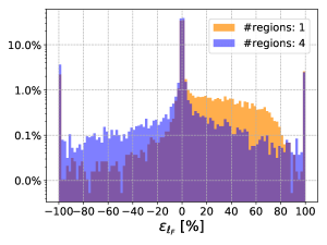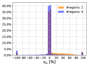
In order to quantify the accuracy of our four-dimensional interpolation strategy we use an adimensional parameter $\epsilon$, which describes the deviation of the interpolated result for the two-loop contribution from its exact expression on a given phase-space point and is defined as

$$\epsilon_{\ell_{\scriptscriptstyle\rm F}}[\%]=\frac{H_{(\text{int})\ell_{\scriptscriptstyle\rm F}}^{{q_{\text{T}}}(2)}-H_{(\text{ex})\ell_{\scriptscriptstyle\rm F}}^{{q_{\text{T}}}(2)}}{H_{(\text{ex})\ell_{\scriptscriptstyle\rm F}}^{{q_{\text{T}}}(2)}}\cdot 100\,,$$ (25)

where the four independent Born flavour configurations $\ell_{\scriptscriptstyle\rm F}=\{q\bar{q},\,\bar{q}q;\;\text{for}\>q\!=\!\text{u-type}\>{\rm or}\;q\!=\!\text{d-type}\}$ have been considered separately. In eq. (25), $H_{(\text{ex})\ell_{\scriptscriptstyle\rm F}}^{{q_{\text{T}}}(2)}$ refers to the hard function in the ${q_{\text{T}}}$-scheme Catani:2013tia returned by Matrix using the evaluation of the exact two-loop coefficients through VVAMP, while $H_{(\text{int})\ell_{\scriptscriptstyle\rm F}}^{{q_{\text{T}}}(2)}$ stands for its value obtained by Matrix using the interpolation of the two-loop coefficients from the precomputed grid results. Note that the conversion between the ${q_{\text{T}}}$-scheme $H_{(\text{int})\ell_{\scriptscriptstyle\rm F}}^{{q_{\text{T}}}(2)}$ and the MiNNLO_PS $H^{(2)}_{\ell_{\scriptscriptstyle\rm F}}$ in section 2.2 has been given in eq. (3.22) of ref. Lombardi:2020wju .

In figure 3, the distribution of the values of $\epsilon_{\ell_{\scriptscriptstyle\rm F}}$ is displayed for a selected flavour channel (namely the $\bar{u}u$ one). All the other flavour channels have the same qualitative behaviour. The figure shows the impact of increasing the number of precomputed grids on the $\epsilon_{\ell_{\scriptscriptstyle\rm F}}$ parameter from one (orange histogram) to four (blue histogram). Besides being essential for a simultaneously accurate description of physical observables over a wide phase-space region, our choice of covering the phase space with four separate grids improves the accuracy of the predictions for the two-loop contribution and yields a more symmetric $\epsilon_{\ell_{\scriptscriptstyle\rm F}}$ distribution.

We further notice that the bulk of the interpolator predictions (roughly $\gtrsim 80\%$) has an accuracy greater than $5\%$ (i.e $|\epsilon_{\ell_{\scriptscriptstyle\rm F}}|\leq 5\%$), while almost $95\%$ lie inside the interval $|\epsilon_{\ell_{\scriptscriptstyle\rm F}}|\leq 100\%$. The remaining fraction of $\epsilon_{\ell_{\scriptscriptstyle\rm F}}$ values consists of phase-space points where the interpolator poorly reproduces the correct two-loop result. In figure 3, where the $\epsilon_{\ell_{\scriptscriptstyle\rm F}}$ distribution is reported both in linear and in logarithmic scale, this fraction is clearly visible in the overflow bins at the edges of the histograms. In most cases, these poorly predicted values are associated to phase-space points falling outside the grid boundaries and thus requiring extrapolation of the two-loop coefficient functions $E_{j}^{[\mathcal{C}],(2)}$ outside the grid edges. However, this also means that most of these points lie in kinematical regions where the cross section is strongly suppressed.

Figure 4: Distribution of the values of the two-loop hard function computed using the interpolator without rescue system for the $\bar{u}u$ channel. In the legend the mean ($\mu$), the median, the standard deviation ($\sigma$) and the skewness ($\gamma_{1}$) are reported. The edge bins account for overflow.

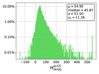
To deal with instabilities, a basic rescue-system is introduced. This mechanism takes care of computing the exact $E_{j}^{[\mathcal{C}],(2)}$ coefficient functions with VVAMP in all cases where $H_{(\text{int})\ell_{\scriptscriptstyle\rm F}}^{{q_{\text{T}}}(2)}$ falls outside a process-specific range, where the bulk of the $H_{(\text{ex})\ell_{\scriptscriptstyle\rm F}}^{{q_{\text{T}}}(2)}$ values lies. Specifically, we have required $-100<H_{(\text{int})\ell_{\scriptscriptstyle\rm F}}^{{q_{\text{T}}}(2)}<500$ as an acceptance interval, where roughly $99.8\%$ of the $H_{(\text{ex})\ell_{\scriptscriptstyle\rm F}}^{{q_{\text{T}}}(2)}$ distribution is concentrated. In figure 4 this distribution is shown together with the median and the value of the first three moments of the distribution. As it can be inferred from the positive skewness value (or from the fact that the mean and median do not coincide), the distribution is asymmetric, which is why our acceptance interval for $H_{(\text{ex})\ell_{\scriptscriptstyle\rm F}}^{{q_{\text{T}}}(2)}$ is not centered around the mean, but rather it extends to higher values to partially account for the long distribution tail on the right of the peak. This simple criterium suffices to catch the small fraction of $\epsilon_{\ell_{\scriptscriptstyle\rm F}}$ outliers that would compromise the stability of the results. Some phase-space points remain that elude the rescue-system and where the two loop coefficients are not computed accurately, but we have checked that they have a negligible impact on the physical results, as it will be discussed below (see figure 6).

Figure 5: Distributions in the evaluation time $t_{\text{\tt VVAMP}}$ (blue histogram) and $t^{\prime}_{\text{int}}$ (orange histogram). The last bin accounts for overflow ($t_{\text{\tt VVAMP}},t^{\prime}_{\text{int}}>20$ s). The left plot resolves the peak of the $t^{\prime}_{\text{int}}$ distribution in double logarithmic scale.

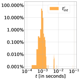
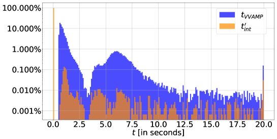
Clearly, the advantage of using the interpolation approach compared to the full evaluation of the two-loop coefficients is the time performance. Indeed, the average time required by VVAMP ($\bar{t}_{\text{\tt VVAMP}}$) and the interpolator ($\bar{t}_{\text{int}}$) to evaluate the two-loop contribution turns out to differ by three orders of magnitude, while the improvement is still roughly a factor forty if one uses the rescue-system ($\bar{t}^{\prime}_{\text{int}}$):

$$\bar{t}_{\text{\tt VVAMP}}\approx 1.9\,{\rm s}\,,\quad\quad\bar{t}_{\text{int}}\approx 0.9\times 10^{-3}\,{\rm s}\,,\quad\quad\bar{t}^{\prime}_{\text{int}}\approx 4.5\times 10^{-2}\,{\rm s}\,.$$ (26)

As complementary information, figure 5 shows the time distributions of $t_{\text{\tt VVAMP}}$ (blue histogram) and $t^{\prime}_{\text{int}}$ (orange histogram). The bulk of the $\tt VVAMP$ evaluation times (roughly $80\%$) is located in the time interval $0.5s<t_{\text{\tt VVAMP}}<2.0$ s, with a small, but not negligible fraction of phase-space points requiring a CPU time between $5.0s<t_{\text{\tt VVAMP}}<7.5$ s, and about $0.1\%$ exceeding $20$ s (visible from the overflow bin). When using the interpolator, more than $99\%$ of the evaluations just require some hundredths of a second. The small number of phase-space points with a CPU time $t^{\prime}_{\text{int}}>0.5$ s are associated to the values catched by the rescue-system. Those timings have been obtained on machines with Intel Haswell Xeon E5-2698 processors with $2.3$ GHz per core.

Figure 6: Powheg stage 2 distributions (from left to right and top to bottom) in ${y_{\text{$WW$}}}$, ${\Delta y_{\text{$W^{-},W^{+}$}}}$, ${y_{\text{$W^{+}$}}}$, ${m_{\text{T,$WW$}}^{\rm exp}}$, ${p_{\text{T,$W^{-}$}}}$ and ${p_{\text{T,miss}}}$ for the VVAMP (blue, solid line), the interpolator (black, dotted line) and the $H^{(2)}_{\ell_{\scriptscriptstyle\rm F}}=0$ (red, dotted line) results.

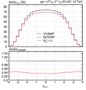
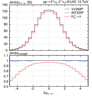
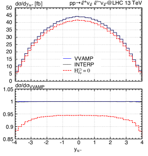
Our implementation of a faster evaluation of the two-loop amplitudes through interpolation is tested by looking at its impact on physical predictions, especially on some relevant differential distributions in the inclusive phase space. All results have been obtained at the level of the Monte Carlo integration of the cross section (i.e Powheg stage 2), so that no parton shower radiation or hadronization effects, which would not be relevant for the validation, have been included.

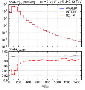
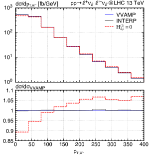
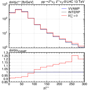
First, it is worth mentioning that the code with the interpolation of the two-loop amplitudes reproduces accurately the exact inclusive cross section, with discrepancies of the order of about $0.4$ permille, which are well within statistical uncertainties. Then, in figure 6 we show representative plots that compare the exact VVAMP predictions (blue, solid line) against the results with interpolation (black, dotted line) for the rapidity of the $W^{+}W^{-}$ pair (${y_{\text{$WW$}}}$), the rapidity difference between the two $W$-bosons (${\Delta y_{\text{$W^{-},W^{+}$}}}$), the rapidity of positively-charged $W$ boson (${y_{\text{$W^{+}$}}}$), the experimental definition of the transverse mass of the $W^{+}W^{-}$ pair

$${m_{\text{T,$WW$}}^{\rm exp}}{}=\sqrt{\left(E_{\text{T,$\ell_{1}$}}+E_{\text{T,$\ell_{2}$}}+{p_{\text{T,miss}}}\right)^{2}-\left({\bf p}_{\text{T,$\ell_{1}$}}+{\bf p}_{\text{T,$\ell_{2}$}}+{\mathbf{{p_{\text{T,miss}}}}}\right)^{2}}\,,$$ (27)

the transverse momentum of the negatively-charged $W$ boson (${p_{\text{T,$W^{-}$}}}$) and the missing transverse momentum (${p_{\text{T,miss}}}$). We stress that many more distributions than those included in this manuscript have been carefully examined and verified to show a very good agreement between the analytic and interpolated results. Moreover, in order to highlight the phase-space regions where the two-loop contribution gives a large contribution to the cross section, a third curve (red, dotted line) has been included in all plots, obtained by setting the MiNNLO_PS $H^{(2)}_{\ell_{\scriptscriptstyle\rm F}}=0$. The lower panel of the plots displays the bin-by-bin ratio using the VVAMP curve as a reference.

From all plots, it is evident that the interpolator reproduces correctly the differential distributions in all kinematical regimes, with only small fluctuations at very high values of ${\Delta y_{\text{$W^{-},W^{+}$}}}$ (at most of the order of $2\%$) or high values of ${m_{\text{T,$WW$}}}$ or ${p_{\text{T,$W^{-}$}}}$ (where differences are well below one percent). These are the regions where the two-loop contribution has the largest impact on the cross section. Indeed, from the ${y_{\text{$WW$}}}$ distribution it is evident that $H^{(2)}_{\ell_{\scriptscriptstyle\rm F}}$ has a $5$-$6\%$ effect on the cross section, and contributes uniformly to this observable, while for instance for $|{\Delta y_{\text{$W^{-},W^{+}$}}}|>4.5$ and $|{y_{\text{$W^{+}$}}}|>4$ it induces a positive correction that reaches more than $30\%$ and $10\%$, respectively. For transverse-momentum distributions, such as ${p_{\text{T,$W^{-}$}}}$ or ${p_{\text{T,miss}}}$, the two-loop contribution has a positive impact for relatively low transverse momenta (roughly for ${p_{\text{T}}}<100$ GeV) of at most $10\%$, while it yields an increasingly negative correction for very large transverse momenta.

3 Phenomenological results

3.1 Input parameters and settings

We consider $\sqrt{s}=13$ TeV proton–proton collisions at the LHC and present predictions for $pp\to\ell^{+}\nu_{\ell}\,\ell^{\prime-}{\bar{\nu}}_{\ell^{\prime}}+X$ production with $\ell=e$ and $\ell^{\prime}=\mu$. The EW parameters are determined in the $G_{\mu}$ scheme, therefore computing the EW coupling as $\alpha_{G_{\mu}}=\sqrt{2}\,G_{\mu}m_{W}^{2}(1-m_{W}^{2}/m_{Z}^{2})/\pi$ and the mixing angle as $\cos\theta_{W}^{2}=m_{W}^{2}/m_{Z}^{2}$. We use the following PDG Patrignani:2016xqp values as inputs: $G_{F}=1.16639\times 10^{-5}$ GeV^-2, $m_{W}=80.385$ GeV, $\Gamma_{W}=2.0854$ GeV, $m_{Z}=91.1876$ GeV, and $\Gamma_{Z}=2.4952$ GeV. We set the CKM matrix to unity, which, because of unitarity and the fact that we consider only massless external quarks is a very good approximation, as explained in ref. Re:2018vac . As described in section 2.1, the four-flavour scheme with $N_{f}=4$ massless quark flavours and massive bottom and top quarks is used to define a top-free $W^{+}W^{-}$ cross section by removing all contributions with final-state bottom quarks. Accordingly, we use the $N_{f}=4$ NNLO set of the NNPDF3.0 Ball:2014uwa parton densities. More precisely, in case of MiNLO^′ and MiNNLO_PS the PDF grids are read from the lhapdf interface Buckley:2014ana , copied into hoppet grids Salam:2008qg and evaluated by hoppet for scales below the internal PDF infrared cutoff through DGLAP evolution with the number of active flavours kept fixed to the one at the internal PDF infrared cutoff, as described in ref. Monni:2020nks . The central renormalization and factorization scales are set following the usual setting for MiNNLO_PS and MiNLO^′ discussed in section 2.3. Perturbative uncertainties are estimated from customary 7-point variations, i.e. by varying ${\mu_{\text{R}}}$ and ${\mu_{\text{F}}}$ around the central scale by a factor of two while respecting the constraint $0.5\leq{\mu_{\text{R}}}/{\mu_{\text{F}}}\leq 2$.

We compare our MiNNLO_PS (and MiNLO^′) predictions to the NNLOPS results presented in ref. Re:2018vac . Those are based on a MiNLO^′ calculation with ${\mu_{\text{R}}}={\mu_{\text{F}}}={p_{\text{T,$WW$}}}{}$, but use NNLO predictions for the reweighting with

$${\mu_{\text{R}}}={\mu_{\text{F}}}=\mu_{\text{0}}\equiv\frac{1}{2}\,\left(m_{\text{T,$W^{+}$}}+m_{\text{T,$W^{-}$}}\right),\quad m_{\text{T,$W^{\pm}$}}=\sqrt{m_{\ell^{(\prime)}\nu_{\ell^{(\prime)}}}^{2}+p^{2}_{{\rm T},\ell^{(\prime)}\nu_{\ell^{(\prime)}}}}\,,$$ (28)

where $m_{\ell\nu_{\ell}}$ and $p_{{\rm T},\ell\nu_{\ell}}$ ($m_{\ell^{\prime}\nu_{\ell^{\prime}}}$ and $p_{{\rm T},\ell^{\prime}\nu_{\ell^{\prime}}}$) are the invariant masses and the transverse momenta of the reconstructed $W$ bosons. The setting in eq. (28) is therefore the effective scale used in the NNLOPS calculation of ref. Re:2018vac , where the perturbative uncertainties are obtained from 7-point scale variations that are assumed correlated in the reweighting. For the ${p_{\text{T,$WW$}}}{}$ spectrum and the jet-vetoed cross section we also compare against more accurate analytically resummed predictions obtained with Matrix+RadISH Kallweit:2020gva ; Wiesemann:2020gbm ; MatrixRadishurl , where we have chosen

$${\mu_{\text{R}}}={\mu_{\text{F}}}=\mu_{\text{0}}\equiv m_{\text{T,$WW$}},\quad Q_{\text{res}}=m_{\text{$WW$}},\quad m_{\text{T,$WW$}}=\sqrt{m_{\text{$WW$}}^{2}+p_{\text{T,$WW$}}^{2}}\,,$$ (29)

with the invariant mass of the $W^{+}W^{-}$ pair ${m_{\text{WW}}}$. Here, scale uncertainties are obtained not just from customary $7$-point variations, but also by varying the resummation scale $Q_{\text{res}}$ by a factor of two around its central value, while keeping ${\mu_{\text{R}}}$ and ${\mu_{\text{F}}}$ fixed to $\mu_{\text{0}}$. For some observables it is instructive to also compare to fixed-order NNLO predictions with both the scale settings in eq. (28) and the ones in eq. (29), which we have obtained with Matrix Grazzini:2017mhc ; Matrixurl . In this case, perturbative uncertainties are again estimated from 7-point scale variations.

As pointed out before, we do not include the loop-induced gluon-fusion contribution in all NNLO results throughout this paper and study the genuine NNLO corrections to the $q\bar{q}$ initiated process. The leading-order gluon-gluon initiated contribution enters at NNLO and NLO QCD corrections to it are known and can be incoherently added to the predictions presented here through a dedicated calculation, which is beyond the scope of this paper. Finally, for the matching to the parton shower we employ Pythia8 Sjostrand:2014zea with a A14 tune TheATLAScollaboration:2014rfk (specifically py8tune 21). Since in this study our focus is on the comparison with other theory predictions, we do not include any effect from hadronization, underlying event models, or a QED shower. Such effects can, however, be directly included and studied by any user of our program through the Pythia8 interface of Powheg-Box-Res.

	fiducial-1-JV Aaboud:2017qkn	fiducial-2-JV Aaboud:2019nkz
Lepton cuts	${p_{\text{T,$\ell$}}}>25$ GeV $|{\eta_{\text{$\ell$}}}|<2.4$	${p_{\text{T,$\ell$}}}>27$ GeV $|{\eta_{\text{$\ell$}}}|<2.5$
	${m_{\text{$\ell\ell$}}}>10$ GeV	${p_{\text{T,}\ell\ell}}>30$ GeV ${m_{\text{$\ell\ell$}}}>55$ GeV
Neutrino cuts	${p_{\text{T,miss}}}>20$ GeV ${p_{\text{T,miss,rel}}}>15$ GeV	${p_{\text{T,miss}}}>20$ GeV
	anti-$k_{\text{T}}$ algorithm with $R=0.4$	anti-$k_{\text{T}}$ algorithm with $R=0.4$
	$N_{\text{jet}}=0$ for ${p_{\text{T,$j$}}}>25$ GeV	$N_{\text{jet}}=0$ for ${p_{\text{T,$j$}}}>35$ GeV
Jet cuts	$|{\eta_{\text{j}}}|<2.5$  ${\Delta R_{\text{$ej$}}}>0.3$
	$N_{\text{jet}}=0$ for ${p_{\text{T,$j$}}}>30$ GeV
	$|{\eta_{\text{j}}}|<4.5$  ${\Delta R_{\text{$ej$}}}>0.3$

Table 1: Fiducial cuts used in two different setups, see text for details.

Since the $W^{+}W^{-}$ cross section is finite at the LO without any cuts, we present results in the fully inclusive $W^{+}W^{-}$ phase space, referred to as setup-inclusive. Additionally, we consider two sets of fiducial cuts, which are summarized in table 1. The first one corresponds to an earlier ATLAS 13 TeV analysis Aaboud:2017qkn and it is identical to that used in the NNLOPS calculation of ref. Re:2018vac , which allows us to compare directly our MiNNLO_PS predictions with the fiducial NNLOPS results of ref. Re:2018vac . We refer to it as fiducial-1-JV in the following. We note that fiducial-1-JV involves a two-fold jet-veto requirement, vetoing all jets in the rapidity region $|{\eta_{\text{j}}}|<2.5$ and separated from the leptons by ${\Delta R_{\text{$ej$}}}>0.3$ with ${p_{\text{T,$j$}}}>25$ GeV and all jets in the rapidity region $|{\eta_{\text{j}}}|<4.5$ and separated from the leptons by ${\Delta R_{\text{$ej$}}}>0.3$ with ${p_{\text{T,$j$}}}>30$ GeV. The second setup instead corresponds to the most recent ATLAS 13 TeV measurement of ref. Aaboud:2019nkz , and it was used to study high-accuracy resummed predictions for $W^{+}W^{-}$ production in ref. Kallweit:2020gva . This setup, referred to as fiducial-2-JV in the following, is useful for two reasons. First, at variance with fiducial-1-JV, it includes a single jet-veto cut for jets with ${p_{\text{T,$j$}}}>35$ GeV. This allows us to directly compare against the NNLO+NNLL resummed predictions for the ${p_{\text{T,$WW$}}}{}$ spectrum with a jet veto Kallweit:2020gva . Note that to facilitate this comparison, we have removed the jet rapidity (${\eta_{\text{j}}}$) requirement from fiducial-2-JV Aaboud:2019nkz , which has a numerically tiny effect. Second, fiducial-2-JV is used to compare against data, since ref. Aaboud:2019nkz measured the fiducial cross section as a function of the jet-veto cut to validate theory predictions for the jet-vetoed $W^{+}W^{-}$ cross section. Let us recall that jet-veto requirements are crucial for experimental $W^{+}W^{-}$ analyses in order to suppress the large top-quark backgrounds. In addition, we introduce fiducial-1-noJV and fiducial-2-noJV for the same fiducial setups as given in table 1, but without any restriction on the jet activity. Those are relevant to study the ${p_{\text{T,$WW$}}}{}$ distribution inclusive over jet radiation as well as the cross section as a function of the jet-veto cut. Besides jet-veto requirements, the two setups in table 1 involve standard cuts on the transverse momentum (${p_{\text{T,$\ell$}}}$) and pseudorapidity (${\eta_{\text{$\ell$}}}$) of the charged leptons as well as a lower cut on the invariant-mass of the dilepton pair (${m_{\text{$\ell\ell$}}}$) and on the missing transverse momentum (${p_{\text{T,miss}}}$). Setup fiducial-2-JV includes also a lower cut on the transverse momentum of the dilepton pair (${p_{\text{T,}\ell\ell}}$), while setup fiducial-1-JV cuts on the so-called relative missing transverse (${p_{\text{T,miss,rel}}}$). The latter denotes the component of the missing transverse momentum vector perpendicular to the direction of the closest lepton in the azimuthal plane, and is defined as

$${p_{\text{T,miss,rel}}}=\left\{\begin{array}[]{ll}{p_{\text{T,miss}}}\cdot\sin|\Delta\phi|&\;\;{\rm for}\;\Delta\phi<\pi/2\,,\\ {p_{\text{T,miss}}}&\;\;{\rm for}\;\Delta\phi>\pi/2\,,\end{array}\right.$$ (32)

where $\Delta\phi$ denotes the azimuthal angle between the missing transverse momentum vector vector and the nearest lepton.

3.2 Integrated cross sections

$\sigma(pp\to\ell^{+}\nu_{\ell}\,\ell^{\prime-}\nu_{\ell^{\prime}})$ [fb]	setup-inclusive	fiducial-1-JV	fiducial-2-JV
MiNLO′	$1156.6(4)_{-5.7\%\phantom{0}}^{+5.4\%\phantom{0}}$	$185.0(2)_{-6.5\%}^{+8.8\%}$	$143.2(2)_{-8.1\%}^{+4.9\%}$
MiNNLOPS	$1292.2(7)_{-0.7\%\phantom{0}}^{+0.6\%\phantom{0}}$	$207.7(2)_{-1.7\%}^{+1.6\%}$	$159.2(4)_{-1.4\%}^{+1.0\%}$
NNLOPS Re:2018vac	$1308.9(3)_{-1.6\%\phantom{0}}^{+1.7\%\phantom{0}}$	$206.4(1)_{-2.3\%}^{+2.2\%}$	$159.0(1)_{-1.8\%}^{+1.7\%}$
NNLO $\mu_{\text{0}}=(m_{\text{T,$W^{+}$}}^{2}+m_{\text{T,$W^{-}$}}^{2})^{0.5}/2$	$1306.5(5)_{-1.6\%\phantom{0}}^{+1.6\%\phantom{0}}$	$206.5(1)_{-0.7\%}^{+1.0\%}$	$158.9(5)_{-0.6\%}^{+0.8\%}$
NNLO $\mu_{\text{0}}=m_{\text{T,$WW$}}$	$1284.9(10)_{-1.3\%}^{+1.4\%}$	—	$160.8(3)_{-0.8\%}^{+1.0\%}$
ATLAS$-gg$ Aaboud:2017qkn	$1481\pm 59\text{(stat)}$	$236.5\pm 10\text{(stat)}$	—
	$\pm 154\text{(syst)}\pm 108\text{(lumi)}$	$\pm 25\text{(syst)}\pm 5.5\text{(lumi)}$
ATLAS$-gg$ Aaboud:2019nkz	—	—	$178.5\pm 2.5\text{(stat)}$
			$\pm 12.7\text{(syst)}\pm 4\text{(lumi)}$
CMS$-gg$ CMS:2016vww	$1289\pm 68\text{(stat)}$	—	—
	${}^{\pm 67\text{(exp.\,syst)}}_{\pm 76\text{(th.\,syst)}}\pm 42\text{(lumi)}$
CMS$-gg$ Sirunyan:2020jtq	$1316\pm 65\text{(stat)}$	—	—
	$\pm 23\text{(syst)}\pm 38\text{(lumi)}$

Table 2: $W^{+}W^{-}$ cross sections in the fully inclusive phase space and in the fiducial phase spaces defined in table 1. We compare our MiNLO^′ and MiNNLO_PS predictions to the NNLOPS results of ref. Re:2018vac and to the NNLO cross section obtained with different settings of ${\mu_{\text{R}}}{}$ and ${\mu_{\text{F}}}{}$. All NNLO corrections to $q\bar{q}$-induced $W^{+}W^{-}$ production are taken into account, while the loop-induced $gg$ contribution is excluded. In the last rows, the comparison to CMS and ATLAS data is shown. For the measured inclusive cross sections we have assumed a branching fraction of $\textrm{BR}(W^{\pm}\rightarrow\ell^{\pm}\nu_{\ell})=0.108987$, consistently evaluated with our inputs, and applied one factor for each of the two $W$ bosons. The measured fiducial cross sections have been divided by a factor two so that they correspond to $pp\to\ell^{+}\nu_{\ell}\,\ell^{\prime-}\nu_{\ell^{\prime}}$ production with $\ell=e$ and $\ell^{\prime}=\mu$. In addition, we have subtracted the loop-induced gluon-fusion contribution from the central value of the data. For the inclusive results and the fiducial-1-JV result we used the prediction for $gg$ (non-resonant) cross section quoted in table 5 of the ATLAS analysis in ref. Aaboud:2017qkn . For the fiducial-2-JV result we used the $gg$LO result in table 2 of ref. Grazzini:2020stb . The ATLAS measurement of ref. Aaboud:2017qkn includes resonant Higgs contributions, which have been subtracted from that data as well, using the corresponding prediction quoted in table 5 of that paper.

We start the presentation of phenomenological results by discussing integrated cross sections in table 2. In particular, we report predictions in the fully inclusive and the two fiducial phase spaces introduced in section 3.1 for MiNLO^′, MiNNLO_PS, NNLOPS Re:2018vac as well as two fixed-order NNLO predictions obtained with Matrix Grazzini:2017mhc ; Matrixurl using the scale settings of eq. (28) and eq. (29). We summarize our main observations in the following:

• It is clear that NNLO accuracy is crucial for an accurate prediction of the $W^{+}W^{-}$ cross section, since the MiNLO^′ result is about 12% lower than the MiNNLO_PS one not only for setup-inclusive, but also after including the fiducial-1-JV and fiducial-2-JV cuts. In fact, in all cases the MiNNLO_PS prediction is outside the upper uncertainty boundary of the MiNLO^′ one. This is not surprising since for $W^{+}W^{-}$ production also at fixed order the NLO uncertainty band does typically not include the central value of the NNLO prediction Grazzini:2016ctr ; Re:2018vac . Additionally, the precision at NNLO is substantially improved, with scale uncertainties reduced by almost an order of magnitude.

• The NNLO-accurate predictions compare well against one another. They are compatible within their respective scale uncertainties and the central predictions are all within less than 2%. Indeed, small differences are expected from the fact that those predictions differ by terms beyond NNLO accuracy. Note that the NNLOPS and the NNLO calculations with $\mu_{\text{0}}=\frac{1}{2}\,\left(m_{\text{T,$W^{+}$}}+m_{\text{T,$W^{-}$}}\right)$ are very close, both in terms of central values and uncertainties, since the former is actually reweighted to the latter prediction in the inclusive phase space. The fact that the inclusive MiNNLO_PS result is about $1.2\%$ below the NNLOPS one is due to the different scale choice and treatment of terms beyond accuracy. Indeed, the second NNLO prediction with a scale choice of $\mu_{\text{0}}={m_{\text{T,$WW$}}}$ is even slightly lower than the MiNNLO_PS one.

• The agreement among predictions with NNLO accuracy gets even better as far as fiducial cross sections are concerned. This could be an indication that the jet vetos that are applied in the fiducial phase spaces reduce the impact of terms beyond NNLO accuracy.

• Some caution is advised regarding the quoted scale uncertainties. First of all, the quoted uncertainties generally appear to be quite small, and potentially at the edge of providing a realistic estimate of the true uncertainty. Clearly, the MiNLO^′ uncertainty does not cover the inclusion of NNLO corrections through MiNNLO_PS. As far as the NNLO-accurate results are concerned, the MiNNLO_PS uncertainties in the inclusive phase space are even a factor of two smaller than the ones of the other predictions. Moreover, the fixed-order NNLO uncertainties further decrease when the jet-veto requirements are imposed. Such behaviour is not new Stewart:2011cf , but at least the showered results show an increased uncertainty when imposing fiducial cuts. Still, especially for the jet-vetoed predictions one may consider more conservative approaches to estimate the perturbative uncertaintes, see for instance refs. Stewart:2011cf ; Banfi:2012jm .

• Finally, there is a good agreement of MiNNLO_PS results with data from ATLAS and CMS in both inclusive and fiducial phase-space regions. The measured cross sections agree mostly within one and at most within two standard deviations.

3.3 Differential distributions

We now turn to discussing differential distributions. We start in section 3.3.1 and section 3.3.2 with comparing our MiNNLO_PS to MiNLO^′ and NNLOPS predictions in the inclusive and the fiducial phase space, respectively. This allows us, on the one hand, to study the effect of NNLO corrections through MiNNLO_PS with respect to MiNLO^′ and, on the other hand, to assess the compatibility of the MiNNLO_PS predictions with the known NNLOPS results. Then in section 3.3.3 we move to distributions sensitive to soft-gluon radiation that require the inclusion of large logarithmic corrections to all orders in QCD perturbation theory either through a parton shower or through analytic resummation.

Unless indicated otherwise, the plots are organized as follows: there is a main frame, which shows differential distributions for the MiNNLO_PS (blue, solid), MiNLO^′ (black, dotted), and NNLOPS (magenta, dash-dotted) predictions. In a lower frame we show bin-by-bin ratios of all curves to the central MiNNLO_PS result. In some cases, where it is instructive to compare to the fixed-order results, we show fixed-order NNLO distributions for $\mu_{\text{0}}=\frac{1}{2}\,\left(m_{\text{T,$W^{+}$}}+m_{\text{T,$W^{-}$}}\right)$ (green, long-dashed) and/or for $\mu_{\text{0}}={m_{\text{T,$WW$}}}$ (red, dashed). We note that we refrain from showing fixed-order NNLO predictions for most observables as the NNLOPS results correspond to a scale setting of $\mu_{\text{0}}=\frac{1}{2}\,\left(m_{\text{T,$W^{+}$}}+m_{\text{T,$W^{-}$}}\right)$ and are, in general, numerically very close to the respective fixed-order NNLO cross section. Additionally, for the ${p_{\text{T,$WW$}}}{}$ distribution we show NNLO+N³LL (green, double-dash dotted) and NNLO+NNLL (brown, dash-double dotted) predictions, and for the ${p_{\text{T,$WW$}}}{}$ spectrum with a jet veto as well as the jet-vetoed cross section we show NNLO+NNLL (green, double-dash dotted) and NLO+NLL (brown, dash-double dotted) results.

3.3.1 Inclusive phase space

Figure 7: Differential distributions in the setup-inclusive.

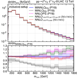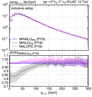
We start by discussing distributions in the inclusive phase space. We have considered a large number of relevant distributions of both the leptonic final states and of the reconstructed $W$-bosons. A selection of those, which reflect some general features, is presented in figure 7. Since experimentally the $W$ bosons can not be directly reconstructed and the fully inclusive phase space can not be covered by the detectors in any case, we follow here a more theoretical motivation and study observables related to the reconstructed $W$ bosons rather than their decay products. In particular, figure 7 shows the transverse-momentum spectrum of the $W^{+}$ boson (${p_{\text{T,$W^{+}$}}}$), the rapidity distribution of the $W$-boson pair (${y_{\text{$WW$}}}$), the rapidity difference between the two $W$ bosons (${\Delta y_{\text{$W^{-},W^{+}$}}}$), and the invariant-mass distribution of the $W$-boson pair (${m_{\text{WW}}}$).

For the ${p_{\text{T,$W^{+}$}}}$ spectrum, the MiNNLO_PS prediction is in full agreement with the NNLOPS result, which is particularly striking in the low-${p_{\text{T,$W^{+}$}}}$ region since scale uncertainties are only at the level of $\pm 1\%$. At larger values of ${p_{\text{T,$W^{+}$}}}$, the uncertainty bands of the NNLO+PS accurate predictions widen and reach about $\pm 5\%$. This indicates that this region is predominantly filled by higher-order (real) radiative corrections with at least one jet, and that the formal accuracy is somewhat decreased by one order. Indeed, in the region ${p_{\text{T,$W^{+}$}}}\gtrsim 100$ GeV the NNLO+PS predictions become fully compatible with the MiNLO^′ result, also in terms of the size of the uncertainty bands. By contrast, for smaller ${p_{\text{T,$W^{+}$}}}$ we observe large NNLO corrections with respect to MiNLO^′ that reach almost $20\%$ and substantially reduced scale uncertainties.

Also for the ${y_{\text{$WW$}}}{}$ and ${\Delta y_{\text{$W^{-},W^{+}$}}}{}$ distributions we find fully compatible results with overlapping uncertainty bands when comparing MiNNLO_PS and NNLOPS predictions. While the NNLO corrections compared to MiNLO^′ are relatively flat for ${y_{\text{$WW$}}}{}$, we find that the corrections increase substantially at larger values of ${\Delta y_{\text{$W^{-},W^{+}$}}}{}$, reaching $\sim+30\%$ for ${y_{\text{$WW$}}}{}\gtrsim 3$. This behaviour was observed already in ref. Re:2018vac and it is reassuring to see that this large effect is not a remnant of the scale setting in the NNLOPS calculation, but a genuine NNLO correction.

Similarly sizeable NNLO corrections are observed also at large values of ${m_{\text{WW}}}$. This is also one of the few regions of phase space that we found where MiNNLO_PS and NNLOPS predictions do not agree at the level of a few percent. While up to ${m_{\text{WW}}}{}\lesssim 500$ GeV the MiNNLO_PS and NNLOPS results are fully compatible, they start deviating at larger invariant masses, reaching differences of about $20\%$ at ${m_{\text{WW}}}{}=1.8$ TeV. Those differences can be traced back to the different scale settings in the MiNNLO_PS and NNLOPS calculations. Indeed, comparing the additional NNLO results shown for the ${m_{\text{WW}}}{}$ distribution, we notice a relatively large spread between the green long-dashed curve with scale setting $\mu_{\text{0}}=\frac{1}{2}\,\left(m_{\text{T,$W^{+}$}}+m_{\text{T,$W^{-}$}}\right)$ and the red dashed curve with $\mu_{\text{0}}={m_{\text{T,$WW$}}}$, which is of the same size as (or even slightly larger than) the observed differences between MiNNLO_PS and NNLOPS. As expected, the NNLOPS result is close to the NNLO one with $\mu_{\text{0}}=\frac{1}{2}\,\left(m_{\text{T,$W^{+}$}}+m_{\text{T,$W^{-}$}}\right)$, while the MiNNLO_PS prediction is somewhat in-between the two NNLO results, but slightly closer to the one with $\mu_{\text{0}}={m_{\text{T,$WW$}}}$. Thus, the origin of the observed differences are terms beyond NNLO accuracy. Although the uncertainty bands increase to about $10\%$ towards large ${m_{\text{WW}}}$, the two NNLO+PS accurate predictions do not (or only barely) overlap for ${m_{\text{WW}}}\gtrsim 1$ TeV, indicating that plain $7$-point scale variations do not represent a realistic estimate of the actual size of uncertainties in that region of phase space. One may ask the question whether one of the two scale choices can be preferred. Although one might assume that ${m_{\text{WW}}}$ would be the natural scale of the ${m_{\text{WW}}}$ distribution, the situation is actually not that clear. This was discussed in some detail in ref. Re:2018vac , and it boils down to the fact that for $s$-channel topologies ${m_{\text{WW}}}$ would be the more natural scale, while for $t$-channel topologies the transverse masses of the W bosons reflect better the natural scale of the process. Since both topologies appear in $W^{+}W^{-}$ production already at the LO and they interfere, it is hard to argue in favour of any of the two scale choices. As a result, and since now there are two NNLO+PS accurate predictions available, the difference between the two should be regarded as an uncertainty induced by terms beyond NNLO accuracy. Moreover, one could introduce a different setting of the hard scales at high transverse momenta in the MiNNLO_PS calculation (i.e. in the $W^{+}W^{-}$+jet part) as a further probe of missing higher-order terms.

In summary, we find that MiNNLO_PS and NNLOPS predictions are in excellent agreement for essentially all observables we considered in the inclusive phase space that are genuinely NNLO accurate. This indicates the robustness of NNLO+PS predictions for such observables. For the few exceptions, like large ${m_{\text{WW}}}$, we could trace back the origin of the differences to terms beyond accuracy that are induced by the different scale settings. Moreover, in all cases the NNLO corrections substantially reduce the scale uncertainties with respect to the MiNLO^′ prediction. Notice, however, that in the bulk region of the inclusive phase space the MiNNLO_PS uncertainty bands are about a factor of two smaller than the NNLOPS ones, as already observed for the fully inclusive cross section.

3.3.2 Fiducial phase space

Figure 8: Differential distributions in the fiducial-1-JV phase space.

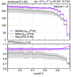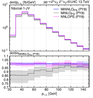
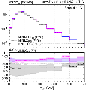
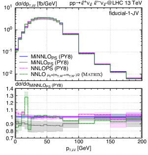
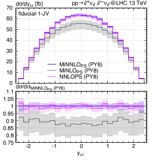
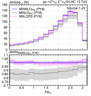
We continue our comparison by considering differential distributions in the fiducial-1-JV phase space. Here, we have selected a set of leptonic observables that are directly measured by the experimental analyses, cf. refs. Aaboud:2017qkn ; Aaboud:2019nkz , and which represent well the general features of all observables we considered. To this end, figure 8 shows the distributions in the transverse momentum of the leading lepton (${p_{\text{T,$\ell_{1}$}}}$), in the invariant mass (${m_{\text{$\ell\ell$}}}$), transverse momentum (${p_{\text{T,}\ell\ell}}$), rapidity (${y_{\text{$\ell\ell$}}}$) and azimuthal difference (${\Delta\phi_{\text{$\ell\ell$}}}$) of the dilepton pair, and in an observable particularly sensitive to new physics effects defined through the separation in $\eta{}$ of the two leptons:

$$\left|\cos(\theta^{\star})\right|=\left|\tanh\left(\Delta\eta_{\ell\ell}/2\right)\right|\,.$$ (33)

As for the setup-inclusive in the previous section, we find full compatibility between MiNNLO_PS and NNLOPS predictions. With fiducial cuts, even the differences induced by terms beyond accuracy are reduced and the scale-uncertainty bands of the two calculations are of similar size. Also in this case, an important observation is that the inclusion of NNLO corrections on top of the MiNLO^′ is crucial not only for the correct normalization, but for many observables also to capture relevant shape effects. Moreover, the NNLO-accurate predictions are substantially more precise due to their strongly reduced uncertainty bands with respect to MiNLO^′. We further notice that the impact of parton-shower emissions on observables with NNLO accuracy is quite moderate. Nevertheless, at phase-space boundaries where the fixed-order accuracy is reduced and the perturbative expansion breaks down due to effects from soft QCD radiation, the parton shower is absolutely crucial for a physical description. For instance, this can observed in the ${p_{\text{T,}\ell\ell}}$ distribution, where we have added the fixed-order NNLO prediction for comparison. Since the ${p_{\text{T,miss}}}>20$ GeV requirement in fiducial-1-JV setup translates directly into a ${p_{\text{T,}\ell\ell}}>20$ GeV cut at LO, where the two leptons are back-to-back with the two neutrinos, the region ${p_{\text{T,}\ell\ell}}\leq 20$ GeV is filled only upon inclusion of higher-order corrections and is effectively only NLO accurate. As a result, the boundary region ${p_{\text{T,}\ell\ell}}\sim 20$ GeV becomes sensitive to soft-gluon effects that induce large logarithmic corrections and a perturbative instability Catani:1997xc at ${p_{\text{T,}\ell\ell}}=20$ GeV in the fixed-order NNLO prediction. This unphysical behaviour is cured through the matching to the parton shower in the MiNNLO_PS and NNLOPS calculations.

It is clear that our new MiNNLO_PS predictions compare very well with the previous NNLOPS results, and that the two tools can be used equivalently to produce $W^{+}W^{-}$ cross sections and distributions at NNLO accuracy matched to parton showers. This is also an indication of the robustness of NNLO+PS predictions for observables that are genuinely NNLO accurate. Given the limitation of the NNLOPS calculation regarding the necessity of multi-dimensional reweighting, the advantage of the MiNNLO_PS generator is that those results can be obtained directly at the level of the event generation. However, in the few phase-space regions where differences between the two calculations can be observed, those differences indicate relevant corrections beyond NNLO accuracy. Since plain $7$-point scale variations do not always cover those discrepancies, they should be regarded as a perturbative uncertainty.

In the next section we will move to observables that are subject to large logarithmic corrections and where differences between the MiNNLO_PS and NNLOPS generator are larger. Thus, their assessment as an uncertainty becomes particularly important.

3.3.3 Observables sensitive to soft-gluon effects

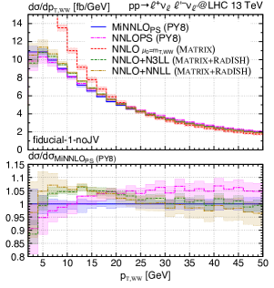
In figure 9, we study the transverse-momentum spectrum of the $W^{+}W^{-}$ pair (${p_{\text{T,$WW$}}}$) in the fiducial-1-noJV phase space. We refrain from showing the corresponding distribution in setup-inclusive and within the fiducial-2-noJV phase space, as we found them to be almost identical concerning the relative behaviour of the various predictions. At small values of ${p_{\text{T,$WW$}}}$, large logarithmic contributions break the validity of the expansion in the strong coupling constant at a given fixed order, which requires their inclusion all orders in perturbation theory either through a parton shower or through an analytic resummation. The left figure displays the region $0\leq{p_{\text{T,$WW$}}}\leq 50$ GeV and, indeed, the NNLO prediction, which is shown in the main frame only, becomes unphysical for small values of ${p_{\text{T,$WW$}}}$. If we compare MiNNLO_PS and NNLOPS results in that region, we observe differences of about $-10$% to $+5$%. By and large, those are covered by the respective uncertainty bands. However, it is clear (and expected) that for such an observable, which is sensitive to infrared physics, the differences between the two calculations become larger. In particular, both predictions are only NLO accurate in the tail of the ${p_{\text{T,$WW$}}}$ distribution and at small transverse momenta the parton shower limits the accuracy of the calculation effectively to leading-logarithmic (LL) or partial (i.e. at leading colour) next-to-LL (NLL) accuracy. Therefore, differences of the order of those that we observe between MiNNLO_PS and NNLOPS are understood. Also the comparison against the high-accuracy analytic resummation results at NNLO+N³LL and NNLO+NNLL is quite good, which also agree within $-10$% to $+5$% with the MiNNLO_PS prediction for ${p_{\text{T,$WW$}}}<20$ GeV and are even fully compatible in the intermediate region up to $50$ GeV. The resummed predictions do not favour either MiNNLO_PS or NNLOPS results, but rather show similar differences to the two. On the other hand, the agreement is actually quite remarkable considering the fact that the region ${p_{\text{T,$WW$}}}<20$ GeV is entirely described by the substantially less accurate parton shower. Given the fact that for some bins the NNLO+N³LL and NNLO+NNLL predictions are outside the uncertainty bands of the NNLO+PS accurate predictions though, the estimated uncertainties from ${\mu_{\text{R}}}$ and ${\mu_{\text{F}}}$ variations appear insufficient to reflect the actual size of uncertainties and one should consider additional handles to better assess the uncertainties of the parton shower at small ${p_{\text{T,$WW$}}}$. Indeed, the NNLL prediction has a much larger uncertainty band in this region (induced by the variation of $Q_{\text{res}}$) even though it is more accurate.

Figure 9: Distribution in the transverse momentum of the $W^{+}W^{-}$ pair in the fiducial-1-noJV phase space, showing a smaller (left plot) and a wider range (right plot).

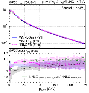In the right plot of figure 9, we show the range $0\leq{p_{\text{T,$WW$}}}\leq 250$ GeV. In the tail of the distribution, MiNNLO_PS and NNLOPS (as well as MiNLO^′) predictions are in perfect agreement with fully overlapping uncertainty bands. In the lower frame we show an additional curve that is ratio of the central fixed-order NNLO prediction with $\mu_{\text{0}}=\frac{1}{2}\,\left(m_{\text{T,$W^{+}$}}+m_{\text{T,$W^{-}$}}\right)$ to the one with $\mu_{\text{0}}={m_{\text{T,$WW$}}}$. It is very interesting to observe that the ratio corresponds almost exactly to the NNLOPS/MiNNLO_PS ratio at smaller ${p_{\text{T,$WW$}}}{}$. We recall that $\mu_{\text{0}}=\frac{1}{2}\,\left(m_{\text{T,$W^{+}$}}+m_{\text{T,$W^{-}$}}\right)$ is the scale used in the reweighting of the NNLOPS prediction, while $\mu_{\text{0}}={m_{\text{T,$WW$}}}$ is somewhat more similar to the one within the MiNNLO_PS approach. This suggests that the differences originating from terms beyond accuracy at small ${p_{\text{T,$WW$}}}{}$ between the MiNNLO_PS and NNLOPS are predominantly induced by the different scale settings in the two calculations. In fact, for any distribution (of the various ones we considered) where the NNLOPS/MiNNLO_PS ratio becomes larger than a couple of percent, we observe that the corresponding ratio of fixed-order NNLO predictions is either very similar or even larger.

Figure 10: Distribution in the transverse momentum of the $W^{+}W^{-}$ pair in the presence of a jet veto (fiducial-2-JV phase space), showing a smaller (left plot) and a wider range (right plot).

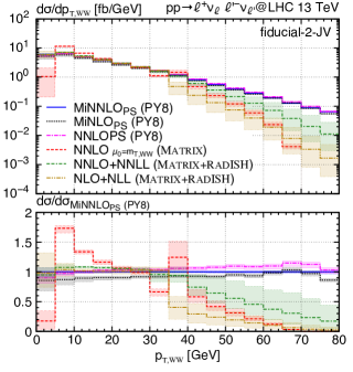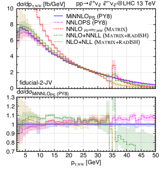
In figure 10 we consider the $W^{+}W^{-}$ transverse momentum spectrum in the presence of a jet veto of ${p_{\text{T,$j_{1}$}}^{\rm veto}}=35$ GeV using the fiducial-2-JV setup. The relative behaviour between the MiNNLO_PS, NNLO+PS, NNLO+NNLL and NLO+NLL results at small transverse momenta is relatively similar to the one observed for the ${p_{\text{T,$WW$}}}{}$ distribution without jet veto in setup fiducial-1-noJV. One main difference is that for this observable, which requires double differential resummation in ${p_{\text{T,$WW$}}}$ and ${p_{\text{T,$j_{1}$}}}$, the analytically resummed results are less accurate and therefore feature larger uncertainty bands, rendering them more compatible with the showered results. Indeed, the NLL uncertainty band is strongly increased at small ${p_{\text{T,$WW$}}}$ and much larger than the NNLO+PS one, which, as argued before, also points to the fact that the scale uncertainties of the latter are somewhat underestimated, given that the parton shower is less accurate than the NLL calculation in that region. Another interesting region for this observable is around ${p_{\text{T,$WW$}}}$ values of $35$ GeV, i.e. of the order of the jet-veto cut. The region ${p_{\text{T,$WW$}}}\geq{p_{\text{T,$j_{1}$}}^{\rm veto}}$ is filled for the first time at NNLO, which is effectively only LO accurate, since at LO it is ${p_{\text{T,$WW$}}}=0$ and at NLO ${p_{\text{T,$WW$}}}={p_{\text{T,$j_{1}$}}}$. Therefore, large logarithmic contributions challenge the perturbative expansion around ${p_{\text{T,$WW$}}}={p_{\text{T,$j_{1}$}}^{\rm veto}}$ and the fixed-order NNLO prediction develops a perturbative instability, as visible in the main frame of the left plot in figure 10. This instability is partially cured by the analytic resummation approach, which resums Sudakov logarithms in the limit where ${p_{\text{T,$WW$}}}$ and ${p_{\text{T,$j_{1}$}}}$ are much smaller than the hard scale, but not all logarithmic contributions of the form $\log({p_{\text{T,$WW$}}}-{p_{\text{T,$j_{1}$}}^{\rm veto}})$, which would require additional resummation when one or more hard jets are present. By contrast, the NNLO+PS calculations cure this instability entirely as they resum all relevant classes of logarithms (although with limited accuracy). Therefore, the MiNNLO_PS and NNLOPS calculations provide a more physical prediction at and above threshold, while below the threshold they are in good agreement with the analytically resummed predictions. If we look at region above threshold in the right plot of figure 10, we notice that the NNLO result drops substantially for ${p_{\text{T,$WW$}}}$ values above ${p_{\text{T,$j_{1}$}}^{\rm veto}}$, and also the NNLO+NNLL prediction is only slightly larger. Hence, this region of phase space is almost exclusively filled by the parton shower. Consequently, the transverse-momentum spectrum of a colour singlet in presence of a jet veto could be a good observable to tune the parton shower in experimental analyses.

Figure 11: Jet-vetoed cross section (left plot) and jet-veto efficiency (right plot) in the fiducial-1-noJV phase space.

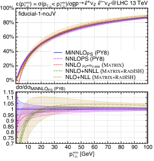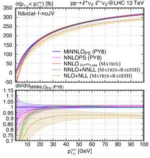
In figure 11 we study the jet-vetoed cross section as a function of the jet-veto cut ${p_{\text{T,$j_{1}$}}^{\rm veto}}$, which is defined as

$$\sigma({p_{\text{T,$j_{1}$}}}<{p_{\text{T,$j_{1}$}}^{\rm veto}})=\int_{0}^{{p_{\text{T,$j_{1}$}}^{\rm veto}}}\mathrm{d}{p_{\text{T,$j_{1}$}}}\,\frac{\mathrm{d}\sigma}{\mathrm{d}{p_{\text{T,$j_{1}$}}}}\,,$$ (34)

and the jet-veto efficiency given by

$$\varepsilon({p_{\text{T,$j_{1}$}}^{\rm veto}})=\sigma({p_{\text{T,$j_{1}$}}}<{p_{\text{T,$j_{1}$}}^{\rm veto}})/\sigma_{\rm int}\,,$$ (35)

where $\sigma_{\rm int}$ is the integrated cross section in the fiducial-1-noJV phase space. Again the results for setup-inclusive and fiducial-2-noJV are very similar and are not shown. The interesting region is at small jet-veto cuts, where the validity of the perturbative expansion is broken by large logarithmic contributions in ${p_{\text{T,$j_{1}$}}^{\rm veto}}$, while for larger values the results tend towards their respective integrated cross sections. As it can be seen from the main frame, in the low ${p_{\text{T,$j_{1}$}}^{\rm veto}}$ region the pure fixed-order result at NNLO becomes indeed unphysical and turns actually negative. When comparing MiNNLO_PS and NNLOPS predictions, we find them to be in reasonable agreement within their respective uncertainties, with the NNLOPS one tending a bit faster towards zero for ${p_{\text{T,$j_{1}$}}^{\rm veto}}\lesssim 20$ GeV. In that region, the resummed NNLO+NNLL and NLO+NLL results tend even faster towards zero, with the NNLO+NNLL curve being about $20\%$ below the MiNNLO_PS one at ${p_{\text{T,$j_{1}$}}^{\rm veto}}=5$ GeV. This region is dominated by the parton shower, which resums only the LL (partial NLL) contributions. Clearly, the actual uncertainties in the NNLO+PS calculations are not covered by plain ${\mu_{\text{R}}}$ and ${\mu_{\text{F}}}$ variations. As argued for the ${p_{\text{T,$WW$}}}{}$ spectrum, additional handles would need to be considered to better assess the parton-shower uncertainties for very small ${p_{\text{T,$j_{1}$}}^{\rm veto}}$ cuts. Indeed, the NLL result features much wider uncertainties, despite being more (similarly) accurate in that region of phase space. However, we stress that such small ${p_{\text{T,$j_{1}$}}^{\rm veto}}$ cuts are usually not relevant for experimental $W^{+}W^{-}$ analyses. Moreover, as pointed out before, there have been suggestions to include more conservative uncertainty estimates for jet-vetoed predictions Stewart:2011cf ; Banfi:2012jm . We leave their proper assessment to future work, as those effects are currently not accessed by any $W^{+}W^{-}$ measurement. For instance, looking at the fiducial phase-space definitions of refs. Aaboud:2017qkn ; Aaboud:2019nkz that are considered in this paper, jet-veto cuts of ${p_{\text{T,$j_{1}$}}^{\rm veto}}=25$ GeV, $30$ GeV and $35$ GeV are used. For those values, MiNNLO_PS predictions are in perfect agreement with the NNLO+NNLL resummation, and even down to ${p_{\text{T,$j_{1}$}}^{\rm veto}}\sim 15$ GeV they differ by less than $5\%$ with overlapping uncertainties.

Figure 12: Jet-vetoed cross section in the fiducial-2-noJV phase space compared to data. As described in the caption of table 2 the data has been adjusted by subtracting the $gg$LO contribution quoted in table 2 of ref. Grazzini:2020stb and by dividing out a factor of two.

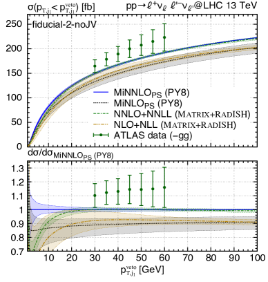
When comparing the predicted jet-vetoed cross section as a function of ${p_{\text{T,$j_{1}$}}^{\rm veto}}{}$ in the fiducial-2-noJV setup against data in figure 12, it is clear that the MiNNLO_PS and the NNLO+NNLL prediction are fully compatible in the relevant region. The agreement with data is good in either case, with the data points either marginally overlapping within one standard deviation or being just outside this range. One should bear in mind however that the normalization of the theory prediction can be increased by $\sim 5$% just by using a different PDF set, which yields even better agreement with data, as shown in ref. Kallweit:2020gva . Apart from that, it is clear that the inclusion of NNLO corrections brings the theory predictions closer to data.

4 Conclusions

In this paper we have presented the matching of NNLO-accurate predictions with parton showers for $W^{+}W^{-}$ production at the LHC using the MiNNLO_PS method. We have performed the calculation consistently in the four-flavour scheme with massive bottom quarks. By dropping contributions with final-state bottom quarks, which are regulated by the finite bottom mass, we generate top-free $W^{+}W^{-}$ events. We have presented an extensive comparison of our MiNNLO_PS predictions against the NNLOPS results of ref. Re:2018vac . We find excellent agreement with the latter results, with only minor differences in phase-space regions where they are expected from the different treatment of terms beyond accuracy, most importantly the ones related to different scale settings. Especially for genuine NNLO observables MiNNLO_PS and NNLOPS are compatible within less than a few percent. Larger differences (but still within uncertainties) can be observed for observables that are sensitive to the limited accuracy of the parton shower, in particular for small values of the $W^{+}W^{-}$ transverse momentum or for very small jet-veto cuts. For those observables we also compared to high-accurate analytically resummed predictions. The agreement is very reasonable considering the limited (leading logarithmic) accuracy of the parton shower. In particular for phase-space regions relevant for experimental $W^{+}W^{-}$ analyses, i.e for jet-veto cuts of $25$ GeV to $35$ GeV (and higher), the MiNNLO_PS prediction essentially coincides with the NNLO+NNLL result. Indeed, we find good agreement both for inclusive and fiducial cross sections with experimental data, as well as for the cross section as a function of the jet-veto cut.

We found that the major bottleneck in the computation is the evaluation of the two-loop amplitude. To improve the speed, we have constructed four-dimensional grids of the coefficients that encode all the information required to reproduce the full two-loop contribution. We then use those grids to obtain the coefficients at any given phase-space configuration through four-dimensional cubic spline interpolation and reconstruct the two-loop amplitude on-the-fly. As a result, the evaluation time of the two-loop contribution has been reduced by a factor of forty, becoming subleading with respect to the other parts of the calculation. We have performed a thorough and extensive validation of the results with interpolation against the ones without. The MiNNLO_PS code can be used either with or without interpolator, the latter option being about five times slower.

The MiNNLO_PS approach has various positive features. First, NNLO corrections are calculated on-the-fly during the generation of the events, with no need for further re-processing or reweighting of the events. Second, no unphysical merging scale needs to be introduced to separate event samples of different multiplicities, a concept already introduced and discussed in detail in ref. Hamilton:2012rf . Third, when combined with transverse-momentum ordered parton showers, the matching guarantees that the logarithmic accuracy of the parton shower simulation is preserved. We note that, because the logarithmic accuracy of parton showers is only leading logarithmic, it is often taken for granted that this accuracy is preserved. On the contrary, this is a subtle, but crucial point in any approach that combines NNLO and parton showers. In the MiNNLO_PS case this requirement is immediately fulfilled for transverse-momentum ordered showers, since zero, one, and two emissions are included in the NNLO weight, where the second-hardest is generated following the Powheg matching procedure, while additional emissions are generated by the parton shower.

We expect that the MiNNLO_PS code associated to the work presented in this paper, which enables an accurate fully-exclusive hadron-level generation of $W^{+}W^{-}$ events, will be highly valuable for experimental measurements, which require an accurate simulation of $W^{+}W^{-}$ production either as signal or as background to other processes. The code will be publicly released within Powheg-Box-Res and will supersede the previous NNLOPS approach based on multi-differential reweighting in Powheg-Box-V2. Nevertheless, we stress that it may be useful to take differences between MiNNLO_PS and NNLOPS predictions (or fixed-order NNLO with different scale settings) to assess residual uncertainties in certain phase-space regimes. Alternatively, different scale settings in the MiNNLO_PS calculation and handles in the parton shower could be used to probe the size of terms beyond accuracy.

Finally, any meaningful comparison to data of differential distributions in charge-neutral vector-boson pair production processes should include not only NNLO QCD accuracy for the $q\bar{q}$ channel, but also NLO QCD corrections to the loop-induced $gg$ process, and possibly NLO EW corrections in the high-energy tails. We leave such studies to future work.

References

- (1) CDF collaboration, T. Aaltonen et al., Measurement of the Production Cross Section and Search for Anomalous and Couplings in Collisions at TeV, Phys. Rev. Lett. 104 (2010) 201801, [0912.4500].
- (2) D0 collaboration, V. M. Abazov et al., Measurement of the WW production cross section with dilepton final states in p anti-p collisions at s**(1/2) = 1.96-TeV and limits on anomalous trilinear gauge couplings, Phys. Rev. Lett. 103 (2009) 191801, [0904.0673].
- (3) D0 collaboration, V. M. Abazov et al., Measurements of and production in + jets final states in collisions, Phys. Rev. Lett. 108 (2012) 181803, [1112.0536].
- (4) ATLAS collaboration, G. Aad et al., Measurement of the cross section in TeV collisions with the ATLAS detector and limits on anomalous gauge couplings, Phys. Lett. B 712 (2012) 289–308, [1203.6232].
- (5) ATLAS collaboration, G. Aad et al., Measurement of production in collisions at =7 TeV with the ATLAS detector and limits on anomalous and couplings, Phys. Rev. D87 (2013) 112001, [1210.2979].
- (6) CMS collaboration, S. Chatrchyan et al., Measurement of the Cross section in Collisions at TeV and Limits on Anomalous and couplings, Eur. Phys. J. C73 (2013) 2610, [1306.1126].
- (7) ATLAS collaboration, G. Aad et al., Measurement of the cross section and limits on anomalous triple gauge couplings using final states with one lepton, missing transverse momentum, and two jets with the ATLAS detector at TeV, JHEP 01 (2015) 049, [1410.7238].
- (8) ATLAS collaboration, G. Aad et al., Measurement of total and differential production cross sections in proton-proton collisions at 8 TeV with the ATLAS detector and limits on anomalous triple-gauge-boson couplings, JHEP 09 (2016) 029, [1603.01702].
- (9) CMS collaboration, S. Chatrchyan et al., Measurement of W+W- and ZZ production cross sections in pp collisions at sqrt(s) = 8 TeV, Phys. Lett. B721 (2013) 190–211, [1301.4698].
- (10) CMS collaboration, V. Khachatryan et al., Measurement of the cross section in pp collisions at 8 TeV and limits on anomalous gauge couplings, Eur. Phys. J. C76 (2016) 401, [1507.03268].
- (11) ATLAS collaboration, M. Aaboud et al., Measurement of production with the hadronically decaying boson reconstructed as one or two jets in collisions at TeV with ATLAS, and constraints on anomalous gauge couplings, Eur. Phys. J. C 77 (2017) 563, [1706.01702].
- (12) ATLAS collaboration, M. Aaboud et al., Measurement of fiducial and differential production cross-sections at TeV with the ATLAS detector, Eur. Phys. J. C79 (2019) 884, [1905.04242].
- (13) ATLAS collaboration, M. Aaboud et al., Measurement of the production cross section in collisions at a centre-of-mass energy of = 13 TeV with the ATLAS experiment, Phys. Lett. B773 (2017) 354–374, [1702.04519].
- (14) CMS collaboration, Measurement of the WW cross section pp collisions at sqrt(s)=13 TeV, CMS-PAS-SMP-16-006.
- (15) CMS collaboration, A. M. Sirunyan et al., W+W- boson pair production in proton-proton collisions at 13 TeV, Phys. Rev. D 102 (2020) 092001, [2009.00119].
- (16) CMS collaboration, S. Chatrchyan et al., Measurement of the and Inclusive Cross Sections in Collisions at TeV and Limits on Anomalous Triple Gauge Boson Couplings, Phys. Rev. D 89 (2014) 092005, [1308.6832].
- (17) CMS collaboration, Measurement of the cross section in pp collisions at sqrt(s) = 8 TeV and limits on anomalous gauge couplings, CMS-PAS-SMP-14-016.
- (18) CMS collaboration, A. M. Sirunyan et al., Search for anomalous couplings in boosted production in proton-proton collisions at 8 TeV, Phys. Lett. B 772 (2017) 21–42, [1703.06095].
- (19) ATLAS collaboration, G. Aad et al., Measurements of jet production cross-sections in collisions at TeV with the ATLAS detector, 2103.10319.
- (20) T. Binoth, M. Ciccolini, N. Kauer and M. Krämer, Gluon-induced background to Higgs boson searches at the LHC, JHEP 0503 (2005) 065, [hep-ph/0503094].
- (21) J. M. Campbell, R. K. Ellis and C. Williams, Gluon-Gluon Contributions to Production and Higgs Interference Effects, JHEP 1110 (2011) 005, [1107.5569].
- (22) ATLAS collaboration, G. Aad et al., Search for the Higgs boson in the lnujj decay channel at TeV with the ATLAS detector, Phys. Lett. B718 (2012) 391–410, [1206.6074].
- (23) ATLAS collaboration, G. Aad et al., Measurements of Higgs boson production and couplings in diboson final states with the ATLAS detector at the LHC, Phys. Lett. B726 (2013) 88–119, [1307.1427].
- (24) CMS collaboration, S. Chatrchyan et al., Measurement of Higgs boson production and properties in the WW decay channel with leptonic final states, JHEP 01 (2014) 096, [1312.1129].
- (25) J. M. Campbell, R. K. Ellis and C. Williams, Bounding the Higgs width at the LHC: Complementary results from , Phys. Rev. D89 (2014) 053011, [1312.1628].
- (26) ATLAS collaboration, G. Aad et al., Observation and measurement of Higgs boson decays to WW∗ with the ATLAS detector, Phys. Rev. D92 (2015) 012006, [1412.2641].
- (27) CMS collaboration, V. Khachatryan et al., Constraints on the spin-parity and anomalous HVV couplings of the Higgs boson in proton collisions at 7 and 8 TeV, Phys. Rev. D92 (2015) 012004, [1411.3441].
- (28) ATLAS collaboration, G. Aad et al., Constraints on the off-shell Higgs boson signal strength in the high-mass and final states with the ATLAS detector, Eur. Phys. J. C75 (2015) 335, [1503.01060].
- (29) ATLAS collaboration, G. Aad et al., Determination of spin and parity of the Higgs boson in the decay channel with the ATLAS detector, Eur. Phys. J. C75 (2015) 231, [1503.03643].
- (30) ATLAS collaboration, G. Aad et al., Study of (W/Z)H production and Higgs boson couplings using decays with the ATLAS detector, JHEP 08 (2015) 137, [1506.06641].
- (31) ATLAS collaboration, G. Aad et al., Measurement of fiducial differential cross sections of gluon-fusion production of Higgs bosons decaying to with the ATLAS detector at TeV, JHEP 08 (2016) 104, [1604.02997].
- (32) F. Caola, M. Dowling, K. Melnikov, R. Röntsch and L. Tancredi, QCD corrections to vector boson pair production in gluon fusion including interference effects with off-shell Higgs at the LHC, JHEP 07 (2016) 087, [1605.04610].
- (33) G. Ferrera, M. Grazzini and F. Tramontano, Associated production at hadron colliders: a fully exclusive QCD calculation at NNLO, Phys. Rev. Lett. 107 (2011) 152003, [1107.1164].
- (34) G. Ferrera, M. Grazzini and F. Tramontano, Associated production at hadron colliders: the fully differential NNLO QCD calculation, Phys. Lett. B740 (2015) 51–55, [1407.4747].
- (35) G. Ferrera, G. Somogyi and F. Tramontano, Associated production of a Higgs boson decaying into bottom quarks at the LHC in full NNLO QCD, Phys. Lett. B780 (2018) 346–351, [1705.10304].
- (36) J. M. Campbell, R. K. Ellis and C. Williams, Associated production of a Higgs boson at NNLO, JHEP 06 (2016) 179, [1601.00658].
- (37) R. V. Harlander and W. B. Kilgore, Higgs boson production in bottom quark fusion at next-to-next-to leading order, Phys. Rev. D68 (2003) 013001, [hep-ph/0304035].
- (38) R. V. Harlander, K. J. Ozeren and M. Wiesemann, Higgs plus jet production in bottom quark annihilation at next-to-leading order, Phys. Lett. B693 (2010) 269–273, [1007.5411].
- (39) R. Harlander and M. Wiesemann, Jet-veto in bottom-quark induced Higgs production at next-to-next-to-leading order, JHEP 04 (2012) 066, [1111.2182].
- (40) S. Bühler, F. Herzog, A. Lazopoulos and R. Müller, The fully differential hadronic production of a Higgs boson via bottom quark fusion at NNLO, JHEP 07 (2012) 115, [1204.4415].
- (41) S. Marzani, R. D. Ball, V. Del Duca, S. Forte and A. Vicini, Higgs production via gluon-gluon fusion with finite top mass beyond next-to-leading order, Nucl. Phys. B800 (2008) 127–145, [0801.2544].
- (42) R. V. Harlander and K. J. Ozeren, Finite top mass effects for hadronic Higgs production at next-to-next-to-leading order, JHEP 11 (2009) 088, [0909.3420].
- (43) R. V. Harlander, H. Mantler, S. Marzani and K. J. Ozeren, Higgs production in gluon fusion at next-to-next-to-leading order QCD for finite top mass, Eur. Phys. J. C66 (2010) 359–372, [0912.2104].
- (44) A. Pak, M. Rogal and M. Steinhauser, Finite top quark mass effects in NNLO Higgs boson production at LHC, JHEP 02 (2010) 025, [0911.4662].
- (45) T. Neumann and M. Wiesemann, Finite top-mass effects in gluon-induced Higgs production with a jet-veto at NNLO, JHEP 11 (2014) 150, [1408.6836].
- (46) D. de Florian and J. Mazzitelli, Higgs Boson Pair Production at Next-to-Next-to-Leading Order in QCD, Phys. Rev. Lett. 111 (2013) 201801, [1309.6594].
- (47) D. de Florian, M. Grazzini, C. Hanga, S. Kallweit, J. M. Lindert, P. Maierhöfer, J. Mazzitelli and D. Rathlev, Differential Higgs Boson Pair Production at Next-to-Next-to-Leading Order in QCD, JHEP 09 (2016) 151, [1606.09519].
- (48) M. Grazzini, G. Heinrich, S. Jones, S. Kallweit, M. Kerner, J. M. Lindert and J. Mazzitelli, Higgs boson pair production at NNLO with top quark mass effects, JHEP 05 (2018) 059, [1803.02463].
- (49) S. Catani, L. Cieri, D. de Florian, G. Ferrera and M. Grazzini, Diphoton production at hadron colliders: a fully-differential QCD calculation at NNLO, Phys. Rev. Lett. 108 (2012) 072001, [1110.2375].
- (50) J. M. Campbell, R. K. Ellis, Y. Li and C. Williams, Predictions for diphoton production at the LHC through NNLO in QCD, JHEP 07 (2016) 148, [1603.02663].
- (51) M. Grazzini, S. Kallweit, D. Rathlev and A. Torre, production at hadron colliders in NNLO QCD, Phys. Lett. B731 (2014) 204–207, [1309.7000].
- (52) M. Grazzini, S. Kallweit and D. Rathlev, and production at the LHC in NNLO QCD, JHEP 07 (2015) 085, [1504.01330].
- (53) J. M. Campbell, T. Neumann and C. Williams, Production at NNLO Including Anomalous Couplings, JHEP 11 (2017) 150, [1708.02925].
- (54) T. Gehrmann, N. Glover, A. Huss and J. Whitehead, Scale and isolation sensitivity of diphoton distributions at the LHC, JHEP 01 (2021) 108, [2009.11310].
- (55) F. Cascioli, T. Gehrmann, M. Grazzini, S. Kallweit, P. Maierhöfer, A. von Manteuffel, S. Pozzorini, D. Rathlev, L. Tancredi and E. Weihs, production at hadron colliders in NNLO QCD, Phys. Lett. B735 (2014) 311–313, [1405.2219].
- (56) M. Grazzini, S. Kallweit and D. Rathlev, ZZ production at the LHC: fiducial cross sections and distributions in NNLO QCD, Phys. Lett. B750 (2015) 407–410, [1507.06257].
- (57) G. Heinrich, S. Jahn, S. P. Jones, M. Kerner and J. Pires, NNLO predictions for Z-boson pair production at the LHC, JHEP 03 (2018) 142, [1710.06294].
- (58) S. Kallweit and M. Wiesemann, production at the LHC: NNLO predictions for and signatures, Phys. Lett. B786 (2018) 382–389, [1806.05941].
- (59) T. Gehrmann, M. Grazzini, S. Kallweit, P. Maierhöfer, A. von Manteuffel, S. Pozzorini, D. Rathlev and L. Tancredi, Production at Hadron Colliders in Next to Next to Leading Order QCD, Phys. Rev. Lett. 113 (2014) 212001, [1408.5243].
- (60) M. Grazzini, S. Kallweit, S. Pozzorini, D. Rathlev and M. Wiesemann, production at the LHC: fiducial cross sections and distributions in NNLO QCD, JHEP 08 (2016) 140, [1605.02716].
- (61) M. Grazzini, S. Kallweit, D. Rathlev and M. Wiesemann, production at hadron colliders in NNLO QCD, Phys. Lett. B761 (2016) 179–183, [1604.08576].
- (62) M. Grazzini, S. Kallweit, D. Rathlev and M. Wiesemann, production at the LHC: fiducial cross sections and distributions in NNLO QCD, JHEP 05 (2017) 139, [1703.09065].
- (63) J. Baglio, A. Djouadi, R. Gröber, M. Mühlleitner, J. Quevillon and M. Spira, The measurement of the Higgs self-coupling at the LHC: theoretical status, JHEP 04 (2013) 151, [1212.5581].
- (64) H. T. Li and J. Wang, Fully Differential Higgs Pair Production in Association With a Boson at Next-to-Next-to-Leading Order in QCD, Phys. Lett. B 765 (2017) 265–271, [1607.06382].
- (65) D. de Florian, I. Fabre and J. Mazzitelli, Triple Higgs production at hadron colliders at NNLO in QCD, JHEP 03 (2020) 155, [1912.02760].
- (66) H. A. Chawdhry, M. L. Czakon, A. Mitov and R. Poncelet, NNLO QCD corrections to three-photon production at the LHC, JHEP 02 (2020) 057, [1911.00479].
- (67) S. Kallweit, V. Sotnikov and M. Wiesemann, Triphoton production at hadron colliders in NNLO QCD, Phys. Lett. B 812 (2021) 136013, [2010.04681].
- (68) S. Kallweit, E. Re, L. Rottoli and M. Wiesemann, Accurate single- and double-differential resummation of colour-singlet processes with MATRIX+RADISH: W+W- production at the LHC, JHEP 12 (2020) 147, [2004.07720].
- (69) S. Frixione and B. R. Webber, Matching NLO QCD computations and parton shower simulations, JHEP 06 (2002) 029, [hep-ph/0204244].
- (70) P. Nason, A New method for combining NLO QCD with shower Monte Carlo algorithms, JHEP 11 (2004) 040, [hep-ph/0409146].
- (71) S. Frixione, P. Nason and C. Oleari, Matching NLO QCD computations with Parton Shower simulations: the POWHEG method, JHEP 11 (2007) 070, [0709.2092].
- (72) K. Hamilton, P. Nason, C. Oleari and G. Zanderighi, Merging H/W/Z + 0 and 1 jet at NLO with no merging scale: a path to parton shower + NNLO matching, JHEP 05 (2013) 082, [1212.4504].
- (73) S. Alioli, C. W. Bauer, C. Berggren, F. J. Tackmann, J. R. Walsh and S. Zuberi, Matching Fully Differential NNLO Calculations and Parton Showers, JHEP 06 (2014) 089, [1311.0286].
- (74) S. Höche, Y. Li and S. Prestel, Drell-Yan lepton pair production at NNLO QCD with parton showers, Phys. Rev. D91 (2015) 074015, [1405.3607].
- (75) P. F. Monni, P. Nason, E. Re, M. Wiesemann and G. Zanderighi, MiNNLO: A new method to match NNLO QCD to parton showers, JHEP 05 (2020) 143, [1908.06987].
- (76) P. F. Monni, E. Re and M. Wiesemann, MiNNLO: optimizing hadronic processes, Eur. Phys. J. C 80 (2020) 1075, [2006.04133].
- (77) J. Mazzitelli, P. F. Monni, P. Nason, E. Re, M. Wiesemann and G. Zanderighi, Next-to-next-to-leading order event generation for top-quark pair production, 2012.14267.
- (78) K. Hamilton, P. Nason and G. Zanderighi, MINLO: Multi-Scale Improved NLO, JHEP 10 (2012) 155, [1206.3572].
- (79) R. Frederix and K. Hamilton, Extending the MINLO method, JHEP 05 (2016) 042, [1512.02663].
- (80) K. Hamilton, P. Nason, E. Re and G. Zanderighi, NNLOPS simulation of Higgs boson production, JHEP 10 (2013) 222, [1309.0017].
- (81) S. Höche, Y. Li and S. Prestel, Higgs-boson production through gluon fusion at NNLO QCD with parton showers, Phys. Rev. D90 (2014) 054011, [1407.3773].
- (82) A. Karlberg, E. Re and G. Zanderighi, NNLOPS accurate Drell-Yan production, JHEP 09 (2014) 134, [1407.2940].
- (83) S. Alioli, C. W. Bauer, C. Berggren, F. J. Tackmann and J. R. Walsh, Drell-Yan production at NNLL’+NNLO matched to parton showers, Phys. Rev. D92 (2015) 094020, [1508.01475].
- (84) W. Astill, W. Bizon, E. Re and G. Zanderighi, NNLOPS accurate associated HW production, JHEP 06 (2016) 154, [1603.01620].
- (85) W. Astill, W. Bizoń, E. Re and G. Zanderighi, NNLOPS accurate associated HZ production with decay at NLO, JHEP 11 (2018) 157, [1804.08141].
- (86) S. Alioli, A. Broggio, S. Kallweit, M. A. Lim and L. Rottoli, Higgsstrahlung at NNLL’NNLO matched to parton showers in GENEVA, Phys. Rev. D100 (2019) 096016, [1909.02026].
- (87) W. Bizoń, E. Re and G. Zanderighi, NNLOPS description of the decay with MiNLO, JHEP 06 (2020) 006, [1912.09982].
- (88) S. Alioli, A. Broggio, A. Gavardi, S. Kallweit, M. A. Lim, R. Nagar, D. Napoletano and L. Rottoli, Resummed predictions for hadronic Higgs boson decays, 2009.13533.
- (89) E. Re, M. Wiesemann and G. Zanderighi, NNLOPS accurate predictions for production, JHEP 12 (2018) 121, [1805.09857].
- (90) D. Lombardi, M. Wiesemann and G. Zanderighi, Advancing MiNNLOPS to diboson processes: production at NNLO+PS, 2010.10478.
- (91) S. Alioli, A. Broggio, A. Gavardi, S. Kallweit, M. A. Lim, R. Nagar, D. Napoletano and L. Rottoli, Precise predictions for photon pair production matched to parton showers in GENEVA, 2010.10498.
- (92) S. Alioli, A. Broggio, A. Gavardi, S. Kallweit, M. A. Lim, R. Nagar and D. Napoletano, Next-to-next-to-leading order event generation for boson pair production matched to parton shower, 2103.01214.
- (93) R. Brown and K. Mikaelian, and Pair Production in , , Colliding Beams, Phys. Rev. D19 (1979) 922.
- (94) J. Ohnemus, An Order calculation of hadronic production, Phys. Rev. D44 (1991) 1403–1414.
- (95) S. Frixione, A Next-to-leading order calculation of the cross-section for the production of pairs in hadronic collisions, Nucl. Phys. B410 (1993) 280–324.
- (96) J. M. Campbell and R. K. Ellis, An Update on vector boson pair production at hadron colliders, Phys. Rev. D60 (1999) 113006, [hep-ph/9905386].
- (97) L. J. Dixon, Z. Kunszt and A. Signer, Vector boson pair production in hadronic collisions at order : Lepton correlations and anomalous couplings, Phys. Rev. D60 (1999) 114037, [hep-ph/9907305].
- (98) L. J. Dixon, Z. Kunszt and A. Signer, Helicity amplitudes for O(alpha-s) production of , , , , or pairs at hadron colliders, Nucl. Phys. B 531 (1998) 3–23, [hep-ph/9803250].
- (99) J. M. Campbell, R. K. Ellis and C. Williams, Vector boson pair production at the LHC, JHEP 07 (2011) 018, [1105.0020].
- (100) A. Bierweiler, T. Kasprzik, J. H. Kühn and S. Uccirati, Electroweak corrections to W-boson pair production at the LHC, JHEP 1211 (2012) 093, [1208.3147].
- (101) J. Baglio, L. D. Ninh and M. M. Weber, Massive gauge boson pair production at the LHC: a next-to-leading order story, Phys. Rev. D88 (2013) 113005, [1307.4331].
- (102) M. Billoni, S. Dittmaier, B. Jäger and C. Speckner, Next-to-leading order electroweak corrections to leptons at the LHC in double-pole approximation, JHEP 1312 (2013) 043, [1310.1564].
- (103) B. Biedermann, M. Billoni, A. Denner, S. Dittmaier, L. Hofer, B. Jäger and L. Salfelder, Next-to-leading-order electroweak corrections to 4 leptons at the LHC, JHEP 06 (2016) 065, [1605.03419].
- (104) S. Kallweit, J. M. Lindert, S. Pozzorini and M. Schönherr, NLO QCD+EW predictions for diboson signatures at the LHC, JHEP 11 (2017) 120, [1705.00598].
- (105) M. Grazzini, S. Kallweit, J. M. Lindert, S. Pozzorini and M. Wiesemann, NNLO QCD + NLO EW with Matrix+OpenLoops: precise predictions for vector-boson pair production, JHEP 02 (2020) 087, [1912.00068].
- (106) E. W. N. Glover and J. J. van der Bij, Z-boson pair production via gluon fusion, Nucl. Phys. B321 (1989) 561–590.
- (107) D. A. Dicus, C. Kao and W. W. Repko, Gluon Production of Gauge Bosons, Phys. Rev. D36 (1987) 1570.
- (108) T. Matsuura and J. van der Bij, Characteristics of leptonic signals for Z boson pairs at hadron colliders, Z. Phys. C51 (1991) 259–266.
- (109) C. Zecher, T. Matsuura and J. van der Bij, Leptonic signals from off-shell Z boson pairs at hadron colliders, Z. Phys. C64 (1994) 219–226, [hep-ph/9404295].
- (110) T. Binoth, N. Kauer and P. Mertsch, Gluon-induced QCD corrections to , Proceedings DIS 2008 (2008) 142, [0807.0024].
- (111) N. Kauer, Interference effects for H WW/ZZ searches in gluon fusion at the LHC, JHEP 12 (2013) 082, [1310.7011].
- (112) F. Cascioli, S. Höche, F. Krauss, P. Maierhöfer, S. Pozzorini and F. Siegert, Precise Higgs-background predictions: merging NLO QCD and squared quark-loop corrections to four-lepton + 0,1 jet production, JHEP 1401 (2014) 046, [1309.0500].
- (113) J. M. Campbell, R. K. Ellis and C. Williams, Bounding the Higgs width at the LHC using full analytic results for , JHEP 04 (2014) 060, [1311.3589].
- (114) J. M. Campbell, R. K. Ellis and C. Williams, Bounding the Higgs Width at the LHC, PoS LL2014 (2014) 008, [1408.1723].
- (115) N. Kauer, C. O’Brien and E. Vryonidou, Interference effects for and searches in gluon fusion at the LHC, JHEP 10 (2015) 074, [1506.01694].
- (116) T. Gehrmann, A. von Manteuffel, L. Tancredi and E. Weihs, The two-loop master integrals for , JHEP 1406 (2014) 032, [1404.4853].
- (117) F. Caola, J. M. Henn, K. Melnikov, A. V. Smirnov and V. A. Smirnov, Two-loop helicity amplitudes for the production of two off-shell electroweak bosons in quark-antiquark collisions, JHEP 1411 (2014) 041, [1408.6409].
- (118) T. Gehrmann, A. von Manteuffel and L. Tancredi, The two-loop helicity amplitudes for leptons, JHEP 09 (2015) 128, [1503.04812].
- (119) R. Poncelet and A. Popescu, NNLO QCD study of polarised production at the LHC, 2102.13583.
- (120) F. Caola, J. M. Henn, K. Melnikov, A. V. Smirnov and V. A. Smirnov, Two-loop helicity amplitudes for the production of two off-shell electroweak bosons in gluon fusion, JHEP 1506 (2015) 129, [1503.08759].
- (121) A. von Manteuffel and L. Tancredi, The two-loop helicity amplitudes for , JHEP 1506 (2015) 197, [1503.08835].
- (122) F. Caola, K. Melnikov, R. Röntsch and L. Tancredi, QCD corrections to production through gluon fusion, Phys. Lett. B754 (2016) 275–280, [1511.08617].
- (123) M. Grazzini, S. Kallweit, M. Wiesemann and J. Y. Yook, production at the LHC: NLO QCD corrections to the loop-induced gluon fusion channel, Phys. Lett. B 804 (2020) 135399, [2002.01877].
- (124) M. Grazzini, S. Kallweit and M. Wiesemann, Fully differential NNLO computations with MATRIX, Eur. Phys. J. C78 (2018) 537, [1711.06631].
- (125) F. Cascioli, P. Maierhöfer and S. Pozzorini, Scattering Amplitudes with Open Loops, Phys. Rev. Lett. 108 (2012) 111601, [1111.5206].
- (126) F. Buccioni, S. Pozzorini and M. Zoller, On-the-fly reduction of open loops, Eur. Phys. J. C78 (2018) 70, [1710.11452].
- (127) F. Buccioni, J.-N. Lang, J. M. Lindert, P. Maierhöfer, S. Pozzorini, H. Zhang and M. F. Zoller, OpenLoops 2, Eur. Phys. J. C 79 (2019) 866, [1907.13071].
- (128) S. Dawson, I. M. Lewis and M. Zeng, Threshold resummed and approximate next-to-next-to-leading order results for pair production at the LHC, Phys. Rev. D88 (2013) 054028, [1307.3249].
- (129) M. Grazzini, S. Kallweit, D. Rathlev and M. Wiesemann, Transverse-momentum resummation for vector-boson pair production at NNLL+NNLO, JHEP 08 (2015) 154, [1507.02565].
- (130) S. Dawson, P. Jaiswal, Y. Li, H. Ramani and M. Zeng, Resummation of jet veto logarithms at N3LLa + NNLO for production at the LHC, Phys. Rev. D94 (2016) 114014, [1606.01034].
- (131) M. Wiesemann, L. Rottoli and P. Torrielli, The Z transverse-momentum spectrum at NNLO+N3LL, Phys. Lett. B 809 (2020) 135718, [2006.09338].
- (132) Matrix+RadISH is an interface to RadISH within Matrix by S. Kallweit, E. Re, L. Rottoli, M. Wiesemann, https://matrix.hepforge.org/matrix+radish.html.
- (133) P. F. Monni, E. Re and P. Torrielli, Higgs Transverse-Momentum Resummation in Direct Space, Phys. Rev. Lett. 116 (2016) 242001, [1604.02191].
- (134) W. Bizon, P. F. Monni, E. Re, L. Rottoli and P. Torrielli, Momentum-space resummation for transverse observables and the Higgs at N3LL+NNLO, 1705.09127.
- (135) P. F. Monni, L. Rottoli and P. Torrielli, Higgs transverse momentum with a jet veto: a double-differential resummation, vol. 124. 2020, 10.1103/PhysRevLett.124.252001.
- (136) P. Jaiswal and T. Okui, Explanation of the excess at the LHC by jet-veto resummation, Phys. Rev. D90 (2014) 073009, [1407.4537].
- (137) P. Meade, H. Ramani and M. Zeng, Transverse momentum resummation effects in measurements, Phys. Rev. D90 (2014) 114006, [1407.4481].
- (138) T. Becher, R. Frederix, M. Neubert and L. Rothen, Automated NNLL NLO resummation for jet-veto cross sections, Eur.Phys.J. C75 (2015) 154, [1412.8408].
- (139) P. F. Monni and G. Zanderighi, On the excess in the inclusive cross section, JHEP 1505 (2015) 013, [1410.4745].
- (140) ATLAS collaboration, Measurement of the production cross section in proton-proton collisions at TeV with the ATLAS detector, ATLAS-CONF-2014-033.
- (141) L. Arpino, A. Banfi, S. Jäger and N. Kauer, BSM production with a jet veto, JHEP 08 (2019) 076, [1905.06646].
- (142) K. Hamilton, A positive-weight next-to-leading order simulation of weak boson pair production, JHEP 01 (2011) 009, [1009.5391].
- (143) J. Bellm, S. Gieseke, N. Greiner, G. Heinrich, S. Plätzer, C. Reuschle and J. F. von Soden-Fraunhofen, Anomalous coupling, top-mass and parton-shower effects in production, JHEP 05 (2016) 106, [1602.05141].
- (144) J. Bellm et al., Herwig 7.0/Herwig++ 3.0 release note, Eur. Phys. J. C76 (2016) 196, [1512.01178].
- (145) S. Hoche, F. Krauss, M. Schonherr and F. Siegert, Automating the POWHEG method in Sherpa, JHEP 04 (2011) 024, [1008.5399].
- (146) P. Nason and G. Zanderighi, , and production in the POWHEG-BOX-V2, Eur. Phys. J. C74 (2014) 2702, [1311.1365].
- (147) T. Melia, P. Nason, R. Röntsch and G. Zanderighi, W+W-, WZ and ZZ production in the POWHEG BOX, JHEP 11 (2011) 078, [1107.5051].
- (148) T. Gehrmann, S. Höche, F. Krauss, M. Schonherr and F. Siegert, NLO QCD matrix elements + parton showers in hadrons, JHEP 01 (2013) 144, [1207.5031].
- (149) S. Höeche, F. Krauss, M. Schonherr and F. Siegert, QCD matrix elements + parton showers: The NLO case, JHEP 04 (2013) 027, [1207.5030].
- (150) R. Frederix and S. Frixione, Merging meets matching in MC@NLO, JHEP 12 (2012) 061, [1209.6215].
- (151) J. Alwall, R. Frederix, S. Frixione, V. Hirschi, F. Maltoni, O. Mattelaer, H. S. Shao, T. Stelzer, P. Torrielli and M. Zaro, The automated computation of tree-level and next-to-leading order differential cross sections, and their matching to parton shower simulations, JHEP 07 (2014) 079, [1405.0301].
- (152) S. Alioli, P. Nason, C. Oleari and E. Re, A general framework for implementing NLO calculations in shower Monte Carlo programs: the POWHEG BOX, JHEP 06 (2010) 043, [1002.2581].
- (153) K. Hamilton, T. Melia, P. F. Monni, E. Re and G. Zanderighi, Merging WW and WW+jet with MINLO, JHEP 09 (2016) 057, [1606.07062].
- (154) S. Bräuer, A. Denner, M. Pellen, M. Schönherr and S. Schumann, Fixed-order and merged parton-shower predictions for WW and WWj production at the LHC including NLO QCD and EW corrections, JHEP 10 (2020) 159, [2005.12128].
- (155) M. Chiesa, C. Oleari and E. Re, NLO QCD+NLO EW corrections to diboson production matched to parton shower, Eur. Phys. J. C 80 (2020) 849, [2005.12146].
- (156) J. C. Collins and D. E. Soper, Angular Distribution of Dileptons in High-Energy Hadron Collisions, Phys. Rev. D 16 (1977) 2219.
- (157)
- (158) Matrix is the abbreviation of Munich Automates qT subtraction and Resummation to Integrate X-sections by M. Grazzini, S. Kallweit, M. Wiesemann, http://matrix.hepforge.org.
- (159) T. Ježo and P. Nason, On the Treatment of Resonances in Next-to-Leading Order Calculations Matched to a Parton Shower, JHEP 12 (2015) 065, [1509.09071].
- (160) T. Binoth, M. Ciccolini, N. Kauer and M. Krämer, Gluon-induced W-boson pair production at the LHC, JHEP 0612 (2006) 046, [hep-ph/0611170].
- (161) N. Kauer and G. Passarino, Inadequacy of zero-width approximation for a light Higgs boson signal, JHEP 1208 (2012) 116, [1206.4803].
- (162) S. Alioli, S. Ferrario Ravasio, J. M. Lindert and R. Röntsch, Four-lepton production in gluon fusion at NLO matched to parton showers, 2102.07783.
- (163) J. Alwall, P. Demin, S. de Visscher, R. Frederix, M. Herquet, F. Maltoni, T. Plehn, D. L. Rainwater and T. Stelzer, MadGraph/MadEvent v4: The New Web Generation, JHEP 09 (2007) 028, [0706.2334].
- (164) J. M. Campbell, R. K. Ellis, R. Frederix, P. Nason, C. Oleari and C. Williams, NLO Higgs Boson Production Plus One and Two Jets Using the POWHEG BOX, MadGraph4 and MCFM, JHEP 07 (2012) 092, [1202.5475].
- (165) G. Cullen et al., GS-2.0: a tool for automated one-loop calculations within the Standard Model and beyond, Eur. Phys. J. C 74 (2014) 3001, [1404.7096].
- (166) J. Campbell and T. Neumann, Precision Phenomenology with MCFM, JHEP 12 (2019) 034, [1909.09117].
- (167) G. P. Salam and J. Rojo, A Higher Order Perturbative Parton Evolution Toolkit (HOPPET), Comput. Phys. Commun. 180 (2009) 120–156, [0804.3755].
- (168) T. Gehrmann and E. Remiddi, Numerical evaluation of harmonic polylogarithms, Comput. Phys. Commun. 141 (2001) 296–312, [hep-ph/0107173].
- (169) P. Nason and C. Oleari, Generation cuts and Born suppression in POWHEG, 1303.3922.
- (170) T. Gehrmann, T. Huber and D. Maitre, Two-loop quark and gluon form-factors in dimensional regularisation, Phys. Lett. B622 (2005) 295–302, [hep-ph/0507061].
- (171) R. J. Gonsalves, Dimensionally Regularized Two Loop On-shell Quark Form Factor, Phys. Rev. D 28 (1983) 1542.
- (172) W. van Neerven, Dimensional Regularization of Mass and Infrared Singularities in Two Loop On-shell Vertex Functions, Nucl. Phys. B 268 (1986) 453–488.
- (173) G. Kramer and B. Lampe, Integrals for Two Loop Calculations in Massless QCD, J. Math. Phys. 28 (1987) 945.
- (174) The Btwxt general-purpose, N-dimensional interpolation library, by N. Kruis, T. Scimone and P. Sullivan, https://github.com/bigladder/btwxt.
- (175) G. Birkhoff and H. L. Garabedian, Smooth surface interpolation, Journal of Mathematics and Physics 39 (1960) 258–268.
- (176) E. Catmull and R. Rom, A class of local interpolating splines, in Computer Aided Geometric Design (R. E. Barnhill and R. F. Riesenfiled, eds.), pp. 317 – 326. Academic Press, 1974. DOI.
- (177) S. Catani, L. Cieri, D. de Florian, G. Ferrera and M. Grazzini, Universality of transverse-momentum resummation and hard factors at the NNLO, Nucl. Phys. B881 (2014) 414–443, [1311.1654].
- (178) Particle Data Group collaboration, C. Patrignani et al., Review of Particle Physics, Chin. Phys. C40 (2016) 100001.
- (179) NNPDF collaboration, R. D. Ball et al., Parton distributions for the LHC Run II, JHEP 04 (2015) 040, [1410.8849].
- (180) A. Buckley, J. Ferrando, S. Lloyd, K. Nordström, B. Page, M. Rüfenacht, M. Schönherr and G. Watt, LHAPDF6: parton density access in the LHC precision era, Eur. Phys. J. C75 (2015) 132, [1412.7420].
- (181) T. Sjöstrand, S. Ask, J. R. Christiansen, R. Corke, N. Desai, P. Ilten, S. Mrenna, S. Prestel, C. O. Rasmussen and P. Z. Skands, An Introduction to PYTHIA 8.2, Comput. Phys. Commun. 191 (2015) 159–177, [1410.3012].
- (182) ATLAS Pythia 8 tunes to 7 TeV datas, ATL-PHYS-PUB-2014-021, 11, 2014.
- (183) I. W. Stewart and F. J. Tackmann, Theory Uncertainties for Higgs and Other Searches Using Jet Bins, Phys. Rev. D 85 (2012) 034011, [1107.2117].
- (184) A. Banfi, P. F. Monni, G. P. Salam and G. Zanderighi, Higgs and Z-boson production with a jet veto, Phys. Rev. Lett. 109 (2012) 202001, [1206.4998].
- (185) S. Catani and B. R. Webber, Infrared safe but infinite: Soft gluon divergences inside the physical region, JHEP 10 (1997) 005, [hep-ph/9710333].