SU(2) lattice gauge theory on a quantum annealer
Abstract
Lattice gauge theory is an essential tool for strongly interacting non-Abelian fields, such as those in quantum chromodynamics where lattice results have been of central importance for several decades. Recent studies suggest that quantum computers could extend the reach of lattice gauge theory in dramatic ways, but the usefulness of quantum annealing hardware for lattice gauge theory has not yet been explored. In this work, we implement SU(2) pure gauge theory on a quantum annealer for lattices comprising a few plaquettes in a row with a periodic boundary condition. These plaquettes are in two spatial dimensions and calculations use the Hamiltonian formulation where time is not discretized. Numerical results are obtained from calculations on D-Wave Advantage hardware for eigenvalues, eigenvectors, vacuum expectation values, and time evolution. The success of this initial exploration indicates that the quantum annealer might become a useful hardware platform for some aspects of lattice gauge theories.
I Introduction
Lattice gauge theory is a mainstay for studies of quantum chromodynamics (QCD) and other strongly coupled gauge theories [1]. Significant computational resources are required, but lattice calculations provide accurate and precise information about many of the interesting properties of nucleons and other hadrons directly from first principles [2]. The lattice QCD research community has a history of evaluating each type of newly available computing hardware for its possible use [3], with an emerging example being qubit-based computing which has produced a lot of enthusiasm and research activity [4]. The first simulations of a lattice gauge theory on digital qubit hardware were reported in Ref. [5] for U(1) with fermions, followed by pure gauge SU(2) [6], pure gauge SU(3) [7], and SU(2) with fermions [8]. Simulations of U(1) gauge theory have also been performed on analog quantum hardware [9, 10, 11]. The pure gauge SU(2) calculations are of particular relevance to the present work, along with many theoretical studies of Hamiltonian SU(2) gauge theory that relate to possible qubit approaches [12, 13, 14, 15, 16, 17, 18, 19, 20, 21, 22, 23, 24, 25, 26, 27, 28, 29, 30, 31, 32, 33, 34, 35]. No lattice gauge theory calculations on a quantum annealer have been reported until the present work, though another group has used a quantum annealer for analyzing lattice QCD results obtained from classical computers [36].
A quantum annealer is a special-purpose type of qubit-based computing device [37, 38, 39]. Review articles can be found in Refs. [40, 41, 42, 43]. D-Wave Systems Inc. [44] has been building quantum annealers for several years, with each generation having a larger number of qubits and increased functionality. The current model has a quantum processing unit (QPU) with 5760 qubits, and each qubit is connected to 15 other qubits to form what is called a Pegasus architecture. Groups of physical qubits can function together as a single “logical qubit,” and these logical qubits can communicate with all-to-all connectivity.
Instead of providing the user with a universal set of quantum gates, the quantum annealer is designed for a specific calculation: finding the ground state of an Ising Hamiltonian (expressed here in the quadratic unconstrained binary optimization or “QUBO” form)
| (1) |
where each binary is 0 or 1 and the user can choose any real-valued coefficients and . The hardware performs its annealing by initializing the system into the ground state of a simple Hamiltonian and then moving quasiadiabatically to the requested Ising Hamiltonian. The Ising model might seem rather far removed from the needs of lattice QCD and too restrictive for any hope of addressing a broad set of observables, but a goal of our paper is to show that this quantum annealer can indeed perform a variety of calculations for a non-Abelian lattice gauge theory. Moreover, the ability to choose directly the coefficients in Eq. (1) is a convenient alternative to what could otherwise be a long sequence of quantum gates on digital hardware.
An appeal of future fault-tolerant universal quantum computers for lattice gauge theory is the potential to open avenues that appear roadblocked to classical computing methods, particularly calculating the evolution of physics in real time and calculating physics in an environment with nonzero baryon density [45]. With classical computers, standard lattice gauge theory algorithms rely on Markov chain Monte Carlo in Euclidean spacetime. The use of Euclidean spacetime offers no access to real-time dynamics. The use of Euclidean Monte Carlo means that nonzero baryon density leads to a complex-valued Monte Carlo probability distribution and therefore a sign problem [46]. Both of these roadblocks can be removed by using a Hamiltonian formulation, but then hardware requirements grow exponentially with the size of the Hilbert space. This is where the hope for a quantum computer comes in: storage of the state vectors in a qubit register can scale polynomially rather than exponentially with the system size, so combining this with an efficient quantum algorithm could lead to practical lattice gauge theory that has access to both real-time dynamics and nonzero baryon density.
Our study does not use the qubit register in a way that achieves polynomial scaling, but the flexibility to easily choose inputs to Eq. (1) does allow for significant classical preprocessing. Therefore the system size for each quantum calculation is only a portion of the physical Hilbert space, with no involvement from any unphysical Hilbert space. This is an approach that is well suited for present-day quantum annealers, leaving the goal of eliminating exponential scaling to be pursued with future hardware. Recall that a quantum annealer can be viewed as a step toward an adiabatic implementation of universal quantum computing [47, 48, 49] which is equivalent to the gate-based implementation [50, 51], though a universal adiabatic implementation might still require more qubits than a gate-based method to achieve the equivalency. References [52, 53] discuss adiabatic quantum computing for lattice gauge theory in a gate-based context.
Besides their connection to future universal quantum computers, quantum annealers should also be compared with classical computers. Classical computation will remain crucial for the development of Hamiltonian lattice gauge theory methods for years to come, and quantum annealing may be a valuable competitor for some tasks. A scaling advantage for quantum annealing relative to path integral Monte Carlo was demonstrated on D-Wave hardware in Ref. [54]. The scaling advantage for a D-Wave QPU relative to classical simulated annealing was demonstrated in Ref. [55]. For examples of speedups attainable by quantum annealing within oracular settings, see Refs. [56, 57]. Error mitigation is also important for maximizing the performance of quantum annealers and this is an active research area [58]. In the present work we will show that, without any special accommodations for optimization or error mitigation, precise results can be obtained for several observables in SU(2) gauge theory on small lattices. Future studies could build on these results to learn how well quantum annealers might eventually perform relative to classical methods.
We have chosen to study the SU(2) case because it is the smallest and simplest non-Abelian gauge theory, but it is worth recalling the long-term motivations as well. SU(2) is a natural first step toward SU(3), which is the gauge group for QCD. SU(2) contributes to the understanding of SU() gauge theories more generally, which helps to frame QCD in a broader perspective. SU(2) is a viable candidate for dark matter if a fermion is added [59, 60].
Various aspects of SU(2) gauge theory have been studied by other researchers who are also using a Hamiltonian formulation that can connect to a qubit implementation [12, 13, 14, 15, 16, 17, 18, 19, 20, 21, 22, 23, 24, 25, 26, 27, 28, 29, 6, 30, 31, 32, 33, 34, 35, 8]. Of particular interest for our work is Ref. [6], which reports the first calculation in SU(2) pure gauge theory on a quantum computer. Specifically, IBM Q Experience gate-based hardware [61] was used to compute several steps in the time evolution of an expectation value on a two-plaquette lattice. That work represents an important milestone for the community, and provides a context in which the results of our present study can be assessed.
Section II of the present work describes the formulation to be used, including the chosen truncation of gauge fields and the number of plaquettes in our lattices. The Hamiltonian matrices are constructed for these lattice systems. Section III shows how spatial symmetries can be used to block diagonalize the Hamiltonian matrices, arriving at a form that will be used as input for the quantum annealer. Section IV presents our use of the D-Wave quantum annealer for computing eigenvalues and eigenvectors as a function of the gauge coupling. Our numerical results are shown to agree with calculations from standard algorithms running on a classical computer. In Sec. V we use the D-Wave quantum annealer to calculate some vacuum expectation values as functions of the gauge coupling, compare them with classical calculations, and use them to determine the systematic effects due to gauge truncation and finite lattice size. Section VI presents a method for computing time evolution and demonstrates its performance on the D-Wave hardware. Section VII contains a summary and outlook. Appendix A contains extra information about deriving the Hamiltonian matrix, Appendix B displays some of the most important blocks from our block diagonalized Hamiltonian matrices, and Appendix C describes the adaptive quantum annealer eigensolver algorithm that we have developed for this project.
II Preparing the Hamiltonian
The Hamiltonian for SU(2) lattice gauge theory was originally derived in Ref. [62]. Follow-up discussions in the context of quantum computing can be found in Refs. [14, 6, 30]. Up to an overall additive constant, the Hamiltonian is
| (2) |
where is the Casimir operator representing the chromoelectric field for the th lattice link. We have suppressed color indices but is the sum over the three (squared) color components of the standard SU(2) Lie algebra, as described, for example, in Refs. [14, 30]. The plaquette operator in Eq. (2) is the trace of the product of four gauge link operators in order (clockwise or counterclockwise) around the th plaquette. The gauge coupling is the only parameter in the Hamiltonian but, following Ref. [14], we have defined
| (3) |
which will be convenient in our work. This coefficient agrees with Ref. [30] but differs from Ref. [6]. We will report energies in units of so graphs of energy versus remain bounded in the strong coupling limit, .
The Hamiltonian formalism uses a spatial lattice rather than the spacetime lattices used for standard Euclidean lattice gauge theory. In the present work we employ a one-dimensional row of 2, 4, or 6 plaquettes with a periodic boundary in the long direction. Figure 1 shows the four-plaquette case.

Because SU(2) is a continuous symmetry, the Hilbert space must be truncated to encode the gauge fields into a finite qubit register. Several formulations have been considered, and Ref. [33] provides a useful comparison of the advantages and disadvantages for some of the leading options. Our work begins from the so-called angular momentum formulation that was also used in Ref. [6] though the implementation is different for a quantum annealer, as will become clear in this paper.
The color state of each gauge link can be represented by a linear combination of basis states where , , 1, , …} identifies the irreducible representation (irrep) of SU(2) while and (half integers between inclusive) are the SU(2) projections at each end of the link. Basis states for the entire lattice are products of these, so a basis state for Fig. 1 can be written as
| (4) |
Color conservation (and the absence of fermions) requires that the three links arriving at any lattice site must form an SU(2) singlet, which corresponds to Gauss’s law.
To apply the Hamiltonian from Eq. (2) to any basis state we need to consider both chromoelectric and plaquette terms. The chromoelectric contribution is easy to evaluate [14] and for Fig. 1 we obtain
| (5) |
Notice that these terms are on the diagonal; a matrix element between unequal states would vanish. The plaquette contribution is a bit more involved but we provide a derivation in Appendix A. For plaquette 1 of Fig. 1, the result is
| (8) | ||||
| (11) | ||||
| (14) | ||||
| (17) |
where and are the SU(2) irreps in and , respectively. The 6j symbols are merely square roots of ratios and are provided in Appendix A. They enforce Gauss’s law automatically. Notice that and will never be the same state because applying a plaquette operator necessarily changes each of those four gauge links by . Therefore all plaquette terms are off diagonal.
The result in Eq. (LABEL:eq:oneplaq) applies to a lattice of any length, not just Fig. 1, because only gauge links comprising or touching the active plaquette (E,F,I,J comprise and A,B,C,D touch) are involved in the calculation. Our Eq. (LABEL:eq:oneplaq) agrees with the expression given in Ref. [6].
Because all sums over the projections and have already been performed to arrive at Eq. (LABEL:eq:oneplaq), any state of the lattice depends only on the irrep values . It is now straightforward to calculate each entry in the Hamiltonian matrix for any one-dimensional periodic lattice of plaquettes. Step 1: Begin with the bare vacuum (all values set to zero) and apply any number of plaquette operators to create all possible new basis states below a chosen maximum value. Step 2: Use Eqs. (2), (5), and (LABEL:eq:oneplaq) to calculate every entry in the Hamiltonian matrix.
Our first example is the case considered in Ref. [6], namely the two-plaquette lattice with each gauge link truncated by , where the Hamiltonian matrix is
| (19) |
The states listed to the right of the matrix identify the rows (and corresponding columns) by using the notation of Fig. 2. Our numerical studies will also go beyond this case in two ways, namely by increasing the length of the lattice and by increasing the cutoff on . Instead of displaying these larger Hamiltonian matrices explicitly, their sizes are listed in Table 1.

| Size of | Size of vacuum block | ||
|---|---|---|---|
| 2 | 1/2 | 44 | 33 |
| 4 | 1/2 | 1616 | 66 |
| 6 | 1/2 | 6464 | 1313 |
| 2 | 1 | 2727 | 1414 |
| 2 | 3/2 | 9595 | 3636 |
| Set label | Number of states | The starting state |
|---|---|---|
| 1 | 1 | |
| 2 | 6 | |
| 3 | 6 | |
| 4 | 6 | |
| 5 | 3 | |
| 6 | 6 | |
| 7 | 6 | |
| 8 | 6 | |
| 9 | 2 | |
| 10 | 6 | |
| 11 | 6 | |
| 12 | 3 | |
| 13 | 6 | |
| 14 | 1 | |
| Total=64 |
III Applying spatial symmetries
Interchanging the states and in Eq. (19) would leave the Hamiltonian matrix invariant. This is a clue to an easy block diagonalization,
| (20) |
For any matrix, performing block diagonalization is valuable because then each block can be submitted to the quantum annealer separately. This reduces the qubit requirements. It also allows the quantum annealer to provide the ground state of each block instead of only providing the ground state of the original matrix.
To generalize the block diagonalization procedure systematically to larger Hamiltonian matrices, we will apply three symmetries to the original lattice basis states: top-to-bottom reflection, left-to-right reflection at a symmetry point, and spatial translation in the periodic (long) direction. It is natural to describe spatial translation by using momentum states via but recall that the coefficients in Eq. (1) need to be real, so a modified approach will be used.
As an example of applying spatial symmetries, consider the lattice with six plaquettes and . The Hamiltonian matrix is 6464 and will not be displayed explicitly here, but we do provide the complete list of 64 basis states in Table 2. These 64 states are collected into 14 sets according to spatial translation symmetry. The notation denotes a state in the th set where the excitation has been translated to the right by sites, so reading from the table immediately tells us that .
Notice that all 64 basis states are symmetric under a top-to-bottom reflection. That will not generally be the case for , but it is true here. If we had chosen and as our example then the states and would have been present. Block diagonalization would have been accomplished by replacing those two states with the linear combinations that are positive and negative under the reflection, i.e., .
The second symmetry to consider for the basis states in Table 2 is left-to-right reflection. Notice that most basis states are symmetric under a left-to-right reflection for some reflection point, but states in sets 7 and 8 are not. Therefore block diagonalization requires replacing pairs of those states with their symmetric and antisymmetric combinations,
| (21) |
The third (and final) symmetry to consider is spatial translation. Invariance under spatial translation leads to conservation of linear momentum, so our Hamiltonian can be block diagonalized into blocks of definite momentum. The six allowed momenta on the six-plaquette lattice are , , , , , and so within the 14 sets of Table 2 we should multiply each state by where is the integer location (i.e. the plaquette number) assigned to the excitation in that state. Only differences in really matter because any extra offset is an irrelevant overall phase. To maintain real coefficients in Eq. (2) we can use the real and imaginary parts separately by introducing the simple factors from Table 3. For the set in Table 2 that contains two basis states, the states to use for block diagonalizing are
| (22) |
which correspond respectively to and . For the sets in Table 2 that contain three basis states, the states to use for block diagonalizing are
| (23) |
which correspond respectively to , real, and imaginary. For the sets in Table 2 that contain six basis states, the states to use for block diagonalizing are
| (24) |
which correspond respectively to , real, imaginary, real, imaginary, and .
Our example of and has now been block diagonalized. The original 6464 Hamiltonian matrix has become two blocks (one 1313 and one 11), a block that is 1818, a block that is 2222, and a pair of blocks (one 77 and one 33). The 1313 block is displayed explicitly in Appendix B.
Because the and blocks each contain forward and backward momenta, their spectra are filled with pairs of degenerate eigenvalues. We can break each of these blocks into two separate blocks by implementing a rotation on pairs of states, so the 1818 block becomes a pair of 99 blocks, and similarly the 2222 block becomes a pair of 1111 blocks.
Classical computing can readily apply spatial symmetries according to the method discussed in this section. Table 1 lists the size of the largest block obtained after block diagonalization for the physics systems to be studied in the present work. Notice that the largest block is always the one containing the bare vacuum state and this block will be of particular interest for computing vacuum expectation values, but every block can be implemented on a quantum annealer to obtain the smallest eigenvalue and its eigenvector.
IV Computing eigenvalues and eigenvectors
The variational method is well known from quantum mechanics as a way to approximate the ground-state wave function and ground-state energy for a given Hamiltonian. By varying the parameters contained in the user’s trial wave function, the best approximation having that particular form can be found. A more general approach is taken here. Specifically, the complete vector space (without choosing any trial wave function) will be discretized in an unbiased way and provided to the quantum annealer, which will then find the desired minimum.
In the standard variational method, the expectation value of a Hamiltonian for any proposed state bounds the ground-state energy according to
| (25) |
with the equality being approached as approaches the true ground state. Notice that for the overly simplistic proposal that each entry in the vector representing is either 0 or 1, we arrive at the Ising ground state of Eq. (1) which is solved by a quantum annealer. [This is true because in Eq. (1).] The general algorithm to be used in our work emerges by applying two extensions. First, a robust numerical implementation needs to handle the possibility of a null vector (=0 ). Second, practical applications need an implementation that can consider any proposed state without restriction to binary entries of 0 and 1. The authors of Refs. [63, 64, 65, 66] have documented an explicit description of this general algorithm and named it the quantum annealer eigensolver (QAE). They have found the QAE to be effective for chemistry calculations on a quantum annealer, and it is also successful for lattice gauge theory as will be demonstrated presently.
The null vector is avoided by adding a penalty term as follows:
| (26) |
where the parameter in the penalty term is adjusted by the user. For a small example, take to be the 33 block in Eq. (20) and use three binary variables to represent .
| 0 | 0 | 0 | 0 | 0 |
|---|---|---|---|---|
| 0 | 0 | 1 | 1 | |
| 0 | 1 | 0 | 1 | |
| 0 | 1 | 1 | 2 | |
| 1 | 0 | 0 | 1 | |
| 1 | 0 | 1 | 2 | |
| 1 | 1 | 0 | 2 | |
| 1 | 1 | 1 | 3 |
All options for are listed in Table 4 but let us begin with the simple case of . Without the penalty term, there are two options for getting the minimum and one of those is the unwanted null vector. Keeping the penalty term means any choice will provide the single normalizable state vector with the correct minimum energy. In practice there is no need to construct the explicit table because if the null vector appears then the user can scan a few values with the quantum annealer to find the transition point where the null vector no longer appears. The appropriate range for is always adjacent to that transition point.
The extension beyond merely 0 and 1 entries in the state vector is accomplished by using multiple binary variables to construct a fixed-point representation. The th entry in the proposed vector state is
| (27) |
where is the number of binary variables used for that entry. Notice that the values are evenly spaced within . On the quantum annealer, one logical qubit is used for each binary variable so finding the ground state for an matrix will use logical qubits. Increasing will increase the precision of the resulting eigenvalue and eigenvector.
To summarize, the state in Eq. (25) is represented by a unit vector which is from Eq. (27) divided by its norm. The original Hamiltonian is used without change. See Appendix C for our implementation.
Calculations on a D-Wave quantum annealer are performed by writing python codes that call D-Wave’s ocean software suite [67]. ocean provides the user with various options to explore optimizations and refinements, including the ability to adjust the annealing schedule which defines how the hardware makes the quasiadiabatic transition from its initial to final Hamiltonian. The default annealing time is 20 microseconds. The default annealing schedule during that 20 microseconds is described in Ref. [68]. We have confirmed that acceptable results are obtained for the present project by using the default time and default schedule. The only hardware parameter we need to adjust is called the chain strength.
A chain is a set of physical qubits within the D-Wave hardware that is used to represent one logical qubit. The length of each chain depends on which connections are required between this particular logical qubit and others. We allow the ocean software to automatically perform the embedding of physical qubits into logical qubits, but we must adjust the chain strength. If the strength is too low then the physical qubits within a logical qubit can disagree with one another and lead to ambiguous physics output. If the chain strength is too high then it competes with the physics terms in the intended calculation and puts a bias on the physics output. The ocean software reports every chain breaking event and this has allowed us to easily tune the chain strength to be within an acceptable range for all of our calculations.
The chain strength is implemented “behind the scenes” by the D-Wave system. Every pair of physical qubits in a chain has an implicit Hamiltonian term of the form where is the Pauli matrix and a subscript identifies a specific physical qubit. The coefficient is the chain strength. Increasing the value of increases the probability that the two qubits will be aligned [69]. For the present study, typical values are between about 1 and 5, tuned at about O(10%).
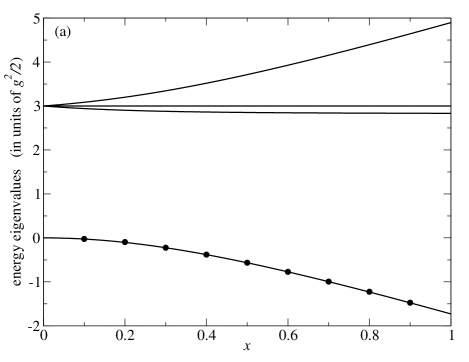
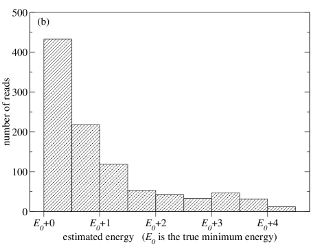
Figure 3(a) shows that the ground-state eigenvalue of Eq. (20) calculated on the D-Wave Advantage quantum annealer is in agreement with classical exact diagonalization of Eq. (20). To make this graph, the coefficient of each basis state for the 33 block of Eq. (20) was represented by seven binary variables, so each quantum calculation used 21 logical qubits. Using somewhat fewer binary variables also gives accurate results, but the D-Wave machine has many qubits available and Fig. 3 confirms that results remain robust even when this larger number of interconnected qubits is used. Our two tunable parameters are and the chain strength, and approximate tuning is sufficient for each of them. The optimal range for is typically slightly above the eigenvalue itself so, when calculating at the sequence of values shown in Fig. 3(a), one can use the eigenvalue obtained at one as the initial estimate for at the neighboring . The chain strength is a positive real value; for this figure we simply used one of the values 1.0, 2.0, 3.0 or 4.0 at each location.
Each of the nine quantum annealing calculations in Fig. 3(a) used “reads” (i.e. annealing cycles) and the graph shows the smallest numerical result from each set of reads, since the smallest is always the best estimator in a variational approach. Each read used 20 microseconds of computing time on the quantum annealer.
Figure 3(b) provides a histogram for the case of where the chain strength was set to 2.0 and 10 of the 1000 reads had broken chains. The histogram contains the 990 unbroken cases. Because the peak of the distribution is in the bin closest to the correct energy, we would be confident of obtaining an accurate result from this quantum annealing calculation even if the classical answer had not been available.
The method used here is immediately applicable to larger physics systems (and we will do so momentarily) because each nonzero entry in any Hamiltonian matrix can be provided directly to the quantum annealer. (Zero entries never need to be provided.) This differs from the approach used in gate-based quantum computing where the Hamiltonian must be expressed as a (possibly long) sequence of quantum gates acting on a qubit register [6, 33]. In addition, gate-based implementations typically include an unphysical sector in the Hilbert space that can be much larger than the physical sector [6, 33] whereas our quantum annealing calculations involve only the physical Hilbert space. These quantum annealing advantages come with the notable cost of requiring many more qubits than are needed by gate-based hardware.
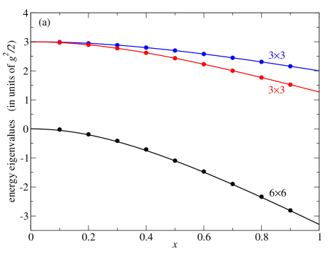
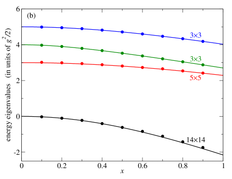
Figure 4 displays the leading corrections arising from (a) a longer lattice and (b) a larger . Specifically, Fig. 4(a) shows the smallest eigenvalue from each block (determined in Sec. III) for the four-plaquette lattice with . The lowest eigenvalue comes from a 66 block and we use reads per value when running on the quantum annealer, but the other blocks are 33 and 1000 reads will suffice for them. The number of logical qubits per entry in the state vector is always .
Figure 4(b) shows the smallest eigenvalue from each block of the two-plaquette lattice with , again choosing . The upper eigenvalues are from a 55 block and two 33 blocks. The lowest eigenvalue comes from a 1414 block where reads is not enough for the original QAE algorithm [63, 64, 65, 66] with . To continue using a maximum of reads per calculation, we have developed an adaptive version of the QAE algorithm (we call it the AQAE algorithm) which runs first with to find an approximate solution, then refines the solution by using on a finer grid in the vicinity of the approximate solution, then zooms in a second time, and then a third time. This AQAE algorithm uses only qubits per entry in the state vector but after three adaptive steps it attains the accuracy of . Additional zooms are possible until the eigenvalue is no longer improved. Data points along the lowest curve in Fig. 4(b) were obtained from the AQAE algorithm with and using between four and nine zooms per value. A distinction between the data points and the exact curve becomes visible on the graph for larger values, but even the data point at only deviates from the exact curve by 4%. Details about the AQAE algorithm are provided in Appendix C.
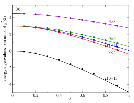
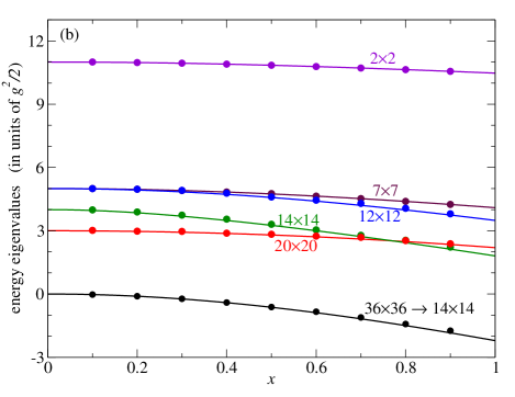
Next-order corrections are obtained by (a) extending the lattice to six plaquettes and (b) extending to . Both of these cases can be studied with our same ocean code and results are displayed in Fig. 5. All of the blocks that generate the excited states in Figs. 5(a) and 5(b) are readily handled by our AQAE algorithm with reads. The lowest block in Fig. 5(a) begins to deviate from the curve as grows, but using more than reads would allow that deviation to shrink. The lowest block in Fig. 5(b) is 3636, and reads are insufficient to see any significant improvement beyond the 1414 results that were already shown in Fig. 4(b). Recalling that the 3636 block contains this exact 1414 matrix, we can conclude that the extra 22 basis states make negligible contributions at the resolution of Fig. 5(b). Therefore we show the same results from the 1414 truncation of the ground state in Figs. 4(b) and 5(b).
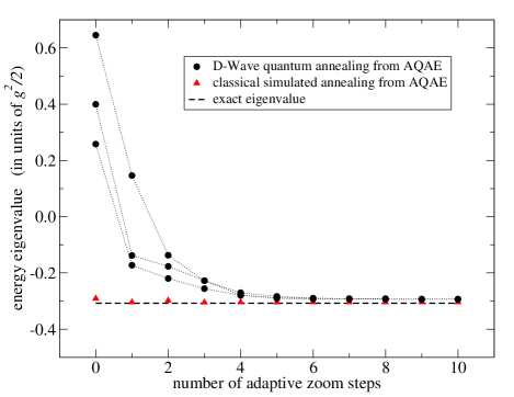
To confirm that our AQAE ocean code is working correctly, the same code was written to run on either the D-Wave quantum annealer or on a laptop with classical simulated annealing by simply changing a single integer flag in the code. We have verified that the output from classical simulated annealing is in excellent agreement with all exact curves, including the full 3636 matrix for Fig. 5(b).
Figure 6 offers an example of how the AQAE algorithm has been vital to the results obtained in this work. Without any adaptive steps, the energy eigenvalue in that graph is clearly far above the correct result when running on D-Wave hardware. There would also be a large error bar as seen by comparing the three separate calculations (each from reads) displayed in Fig. 6. The first adaptive step provides a major improvement and successive steps continue to approach the true result, thus allowing the completion of Figs. 4 and 5 where statistical error bars are smaller than the data symbols. In contrast, the adaptive steps provide smaller improvements when calculating with a classical simulator. Figure 6 shows that classical simulated annealing from the original QAE algorithm (corresponding to no adaptive zoom steps) is already within about 5% of the correct result.
V Computing vacuum expectation values
The particles contained within SU(2) pure gauge theory are called glueballs, and their energies are obtained from differences between the eigenvalues calculated in Sec. IV, , where is the smallest eigenvalue. The symmetries implemented in Sec. III identify the specific parity and momentum corresponding to each . Physically interesting glueball energies would be obtained from computations on larger lattices closer to the continuum limit, which is approached as the inverse gauge coupling is increased.
The calculations in Sec. IV produced eigenvectors as well as eigenvalues, and the eigenvector corresponding to represents the theory’s vacuum state. This provides access to the calculation of the vacuum-to-vacuum matrix elements that are so important in quantum field theory. In this section, vacuum expectation values are computed and used to probe the systematic effects due to lattice volume and the truncation.
Because we cannot use an infinite number of qubits, there is always some limit to the precision of any calculation. For the variational method, these uncertainties are for the eigenstates but for the eigenvalues, where represents a perturbation. Therefore we can anticipate less precise results for vacuum expectation values than for the associated eigenvalue.
Recall from Eq. (2) that the general SU(2) Hamiltonian is the sum of a chromoelectric term and a plaquette term, where the continuum limit of the plaquette term contains a chromomagnetic contribution and an additive constant. In units of , the vacuum expectation value of Eq. (2) can be written as
| (28) |
To the left of the equal sign is the smallest eigenvalue. The first(second) term on the right side can be calculated by matrix multiplication using the diagonal(off-diagonal) terms in the Hamiltonian together with the ground-state eigenvector that was computed in Sec. IV.
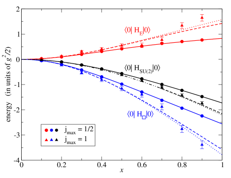
Figure 7 shows the three terms of Eq. (28) on a two-plaquette lattice for the available values, with data points obtained from the quantum annealer and curves obtained classically. Data points show small but visible deviations from the classical curves for the chromoelectric and plaquette terms separately but, as anticipated, their sum is equal to the minimum eigenvalue and is closer to its classical curve. Data points for do not appear on the graph because, as discussed in Sec. IV, those D-Wave results are not significantly resolved from the data points.
The full effects of gauge fields are attained as , and the comparison of different choices in Fig. 7 suggests a rapid convergence for the range of gauge couplings studied here, . The precise rate of convergence always depends on the particular observable being considered, and we see that calculations for and are closer together for the full Hamiltonian than for the chromoelectric or plaquette terms separately.
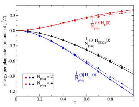
To determine how results depend on lattice volume, it is convenient to divide Eq. (28) by the number of plaquettes, thereby obtaining an energy density. Classical calculations show no visible distinction between and 6 at the resolution of Fig. 8 so they appear as a single dot-dashed curve. The two-plaquette result is a nearby solid curve. Taken together, the three volumes show that these energy densities (chromoelectric, plaquette, and total) are indeed local quantities with no significant dependence on lattice volume beyond a few plaquettes, at least for the range of considered here. As expected, computations on the D-Wave quantum annealer in Fig. 8 show smaller errors for the total energy than for the separate chromoelectric and plaquette terms.
VI Computing time evolution
Time evolution is a key motivation for using the Hamiltonian approach because traditional lattice gauge theory calculations employ Euclidean time and thus lack access to real-time dynamics. For quantum computing, real-time evolution can be handled with the Suzuki-Trotter approach [70, 71], where is applied repeatedly for a small time step , and denotes the Hamiltonian operator. Since a quantum annealer does not provide gates from which to build an operator, time evolution must instead be translated into a ground-state eigenvalue problem. This can be accomplished by using Kitaev-Feynman clock states [72, 73] that were also used, for example, to show the equivalence of adiabatic quantum computing to gate-based quantum computing [50, 51].
The basic idea is that a sequence of time values is defined, and the quantum annealer will calculate the minimum eigenvalue for the entire time sequence at once, thereby giving the state of the system at all times. A clear derivation can be found in Ref. [74] where the approach is called the time-embedded discrete variational principle (TEDVP). Reference [74] shows that the functional to be minimized is
| (29) |
where is the state of the system at time , is the state of the clock at time , and the clock Hamiltonian is
| (30) | |||||
where performs the evolution from to and is a penalty term used to specify the initial state at time . Because Eq. (29) has the same form as Eq. (26) up to an additive constant, we can apply the QAE directly to the TEDVP calculation of time evolution. Notice that the clock Hamiltonian acts on a compound state built from both the physical state and the clock state. The compound state is larger than the physical state by a factor of the number of time steps, so the number of qubits required will increase by this same multiplicative factor.
Implementing a QAE+TEDVP algorithm on the quantum annealer is hampered by imaginary terms in because the D-Wave hardware needs real entries throughout Eq. (1). We will handle this by working in a basis where the Hamiltonian is purely imaginary.
Consider the case of a two-plaquette lattice that is described sufficiently accurately by the truncated Hamiltonian shown in Eq. (20). The 33 block describes the ground state plus two excited states, and we want to calculate the oscillation between those two excited states as a function of time. As indicated by the labels in Eq. (20), this will be oscillation between a superposition of single-plaquette excitations and a pair of round-the-world excitations . Both options have exactly four excited gauge links, so they are exactly degenerate at and nearly degenerate for small .
There is no change of basis that converts this 33 block into a 33 imaginary matrix. However, in the strong coupling (small ) region where Eq. (20) applies, we can augment it with an additional heavy state to form this matrix,
| (31) |
that can be written (up to a constant) in a purely imaginary form,
| (32) |
| (33) |
Since our calculation of oscillations will only depend on energy differences, the constant can be subtracted from Eq. (32), leaving an imaginary matrix that is block diagonal. The block with contains the ground state and the fictitious heavy state. The block with contains the two intermediate states that are of interest to us, and its time evolution is represented by
| (34) |
where .
Note that, for small , the effect of adding the fictitious heavy state [which has the value 6 on the diagonal of Eq. (31)] is smaller than the effect of truncating the Hamiltonian matrix down to its 33 form [because Eq. (129) has values smaller than 6 on the diagonal that must be truncated to arrive at the 33 form]. Therefore, since we are considering an example where the 33 truncation is sufficiently accurate, we are justified to add the heavy state.
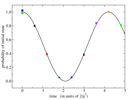
It is now straightforward to implement our QAE+TEDVP code on D-Wave hardware. However, today’s quantum annealers are only intended to handle situations that do not have sign problems. Specifically, D-Wave hardware is designed to handle “stoquastic” Hamiltonian matrices, which have only nonpositive off-diagonal elements in the computational basis [69], but Eq. (30) does not have this form when is given by Eq. (34) with an arbitrary time step . Figure 9 presents the output from several runs of our code that used only two times each: and a larger . With two states at two times and , each computation used 28 logical qubits. To obtain the precision of Fig. 9, we used reads. However, even noisy data would be sufficient to provide a useful estimate of the frequency directly from the D-Wave data. This is valuable because we can then choose the truly stoquastic case of for followup computations, where D-Wave hardware will handle time evolution well.
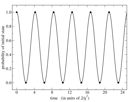
Figure 10 shows 12 time values obtained from a single run of stoquastic time evolution using our QAE+TEDVP algorithm on the D-Wave Advantage hardware. This computation used for each of the two states at each of 12 time values for a total of 48 logical qubits. The physical energy gap between the two oscillating states can be extracted as .
For an indication of how D-Wave hardware performance has been improving, we compare our findings with Fig. 1 of Ref. [75]. In that work, a similar method was used to observe Rabi oscillations by using the previous two generations of D-Wave annealers, the original 2000Q (released in 2017) and the low-noise 2000Q (released in 2019). The authors of Ref. [75] used those machines to attain five time values and six time values respectively in their Rabi oscillation computations. Our study has used the newer Advantage hardware (released in 2020) to attain 12 time values in Fig. 10.
VII Summary and outlook
In this work, we have used a D-Wave quantum annealer to compute several quantities in a non-Abelian gauge theory. Although the annealer is designed to focus on the optimization problem for an Ising model, we have demonstrated computations in SU(2) lattice gauge theory for eigenvalues, eigenvectors, vacuum expectation values, and real-time evolution. Quantum computing is presently in an era of noisy qubits, but the graphs in Figs. 3-10 demonstrate that a quantum annealer can already produce results that are reasonably precise and accurate, at least on lattices having only a few plaquettes.
For the one-dimensional plaquette lattices studied in this work, classical preprocessing readily produced the explicit Hamiltonian matrices, and then translation and reflection symmetries were used to block diagonalize those matrices. The QAE algorithm [63, 64, 65, 66] allowed each of those blocks to be entered directly into the quantum annealer without the need to construct them from products of quantum gates. The D-Wave hardware readily determined respectable results for the lowest eigenvalue and eigenvector from each of the smaller blocks. To extend this success to larger blocks, we developed an adaptive QAE algorithm which is presented in Appendix C. The D-Wave ocean software [67] offers several methods for tuning hardware performance and enhancing results, but we obtained good quality output without these aids, retaining only the two mandatory adjustable quantities: the penalty parameter of QAE and the chain strength of D-Wave. Each of our calculations needed only a portion of the physical Hilbert space, and no unphysical Hilbert space was present.
Real-time oscillations between two excited states were also computed on the quantum annealer. The basic approach was to use Kitaev-Feynman clock states [72, 73] and we implemented these by combining the QAE with the TEDVP [74]. Besides demonstrating the ability to access time evolution on a quantum annealer, our QAE+TEDVP computation is also a method for measuring the energy splitting between excited states.
Our choice to begin with SU(2) pure gauge theory on a two-plaquette lattice follows the work of Ref. [6], where the same system was studied on a gate-based quantum computer. Our work goes beyond that starting point in two ways: by extending the number of plaquettes from to 4 and 6, and by increasing the gauge field truncation from to 1 and . For the range of gauge couplings in our work, calculations at these sequences of and values indicate that contributions which would have arisen from still larger and values are negligible. All of our Hamiltonians were straightforward to implement on the quantum annealer because each new matrix can be encoded directly, without any decomposition into gates, but this advantage comes at the expense of requiring many more qubits than the gate-based approach of Ref. [6].
Gate-based quantum computers have the ability to store a quantum state more efficiently than classical computers, and this will be very significant for lattices that are large enough to address the intended goals of nuclear and particle physics phenomenology. Indeed, this state-storage scaling advantage is a key motivator for Ref. [6] and for the entire field of quantum computation in lattice gauge theories. If quantum annealers are to compete with gate-based hardware, then the storage scaling issue must be addressed by quantum annealers as they continue to evolve toward a fully universal form of adiabatic quantum computing. That will be an important challenge for future algorithms on future adiabatic hardware but, independently, near-term quantum annealers might be useful alongside gate-based hardware in complementary rather than competitive ways. For example, some algorithms relevant to lattice gauge theory might achieve a speedup sufficient to supersede classical computers [54, 55, 56, 57], making quantum annealers a useful tool during the next several years of study on intermediate-sized lattices. To assess the power of quantum annealing, further experiments are called for [76], and our work is a step along this path. As quantum hardware continues to evolve rapidly, we anticipate that mutually complementary roles could emerge for several quantum and classical hardware platforms within the broad scope of lattice gauge theory research.
Appendix A Deriving the plaquette term
To derive Eq. (LABEL:eq:oneplaq), begin with the constraint of Gauss’s law at lattice site 1 of Fig. 1, which says the three gauge links form a color singlet, , giving
| (35) | |||||
| (36) | |||||
| (37) | |||||
| (40) |
where our convention is to use for the left or bottom end of a link and to use for the right or top end. The other seven vertices have similar expressions,
| (43) | |||||
| (46) | |||||
| (49) | |||||
| (52) | |||||
| (55) | |||||
| (58) | |||||
| (61) |
The product of the eight vertex states defines the state of the entire lattice. Notice that we always list the gauge links through in alphabetical order so the calculation will be self-consistent and have the correct Clebsch-Gordan phases. The labeling of gauge links chosen in Fig. 1 (even horizontal, then odd horizontal, then vertical) is not required, but it does maintain a convenient pattern among the four plaquette operators during the derivations. The first plaquette operator is
| (62) |
where each sum includes only the two terms . Notice that the subscripts on and have been interchanged because going counterclockwise around the plaquette means we are going from the end to the end on those two links. The effect of an operator is [14, 6]
| (63) | |||||
| (68) |
where the sums over and contain only a single nonzero term because the Clebsch-Gordan coefficients vanish unless and . Applying to our initial state gives
| (105) | |||||
Applying a final state to that result allows all sums to be performed and the answer simplifies to
| (114) | |||||
as given in Eq. (LABEL:eq:oneplaq). Results for with can be obtained simply by translation symmetry from the result or by explicit calculation.
Appendix B VACUUM SECTOR MATRICES
As explained in Sec. III, three spatial symmetries can be used to block diagonalize each Hamiltonian matrix. One explicit example was provided in Eq. (20). The largest blocks that arise from three additional physics systems are provided here. Recall that the largest block is always the one containing the vacuum state.
For and , the vacuum block is
| (127) |
with the basis states shown beside their corresponding rows. For and , the vacuum block is
| (128) |
with the basis states shown beside their corresponding rows in the notation of Sec. III and the extra shorthand notation . For and , the vacuum block is
| (129) |
where the basis states, in order from top to bottom, are
| (130) |
The presence of a positive off-diagonal entry in Eq. (129) suggests that the matrix is not perfectly suited for today’s D-Wave hardware [69], but it does not represent any sign problem in the underlying theory and we can obtain accurate numerical results on D-Wave as discussed in Sec. IV.
Appendix C THE AQAE ALGORITHM
The quantum annealer eigensolver was defined by Teplukhin et al. in Ref. [63] to solve the eigenvalue problem for a real symmetric matrix on a quantum annealer. It was later augmented with an automated search for [the penalty parameter that appears for example in our Eq. (26)] [64] and was also extended to accommodate complex matrices [65]. Classical algorithms for splitting larger QUBO problems into smaller ones for use with QAE were assessed in Ref. [66]. In the present work we introduce an adaptive search.
In our adaptive QAE algorithm, the standard QAE algorithm runs several times in sequence, with the best eigenvector from one run being used as input for the next. The original run searches within the set of vectors having real components and it uses qubits to give equally spaced options for each . Every subsequent run uses the same number of qubits but searches a range for each that is half of the previous size, so the allowed values are more finely spaced. That smaller range is centered on the best value obtained from the previous run. Our AQAE algorithm is outlined below, using some notation from the Supporting Information that accompanies Ref. [63].
Begin with the vector set to zero, which is the center of the initial range ,
| (131) |
Now loop all remaining steps, i.e. Eqs. (135)-(139), over the sequence of QAE runs while increasing the “zoom factor” for each subsequent run,
| (132) | |||||
| (135) | |||||
| (136) | |||||
| (138) | |||||
| (139) |
where is the number of rows in the matrix and is the number of logical qubits to be used. The quantities are the binary variables that we introduced in Sec. IV. The quantity was defined in Eq. (26) and is the dataset that gets provided directly to the D-Wave quantum annealer. The iteration can be terminated after any quantum annealing step, for example when subsequent values are no longer providing an improved (i.e. smaller) ground-state eigenvalue.
Acknowledgements.
We are grateful to D-Wave Systems Inc. (Burnaby, Canada) for providing us with computing time on their quantum annealing hardware. Our work was supported in part by a Discovery Grant from the Natural Sciences and Engineering Research Council (NSERC) of Canada. S.A. received additional funding from a Dean’s Undergraduate Research Award, E.M. from a Carswell Graduate Scholarship, and S.P. from an NSERC Undergraduate Student Research Award.References
- Brambilla et al. [2014] N. Brambilla et al., QCD and Strongly Coupled Gauge Theories: Challenges and Perspectives, Eur. Phys. J. C 74, 2981 (2014), arXiv:1404.3723 [hep-ph] .
- Kronfeld [2012] A. S. Kronfeld, Twenty-first Century Lattice Gauge Theory: Results from the QCD Lagrangian, Ann. Rev. Nucl. Part. Sci. 62, 265 (2012), arXiv:1203.1204 [hep-lat] .
- Rago [2018] A. Rago, Lattice QCD on new chips: a community summary, EPJ Web Conf. 175, 01021 (2018), arXiv:1711.01182 [hep-lat] .
- Bañuls et al. [2020] M. Bañuls et al., Simulating Lattice Gauge Theories within Quantum Technologies, Eur. Phys. J. D 74, 165 (2020), arXiv:1911.00003 [quant-ph] .
- Martinez et al. [2016] E. Martinez, C. Muschik, et al., Real-time dynamics of lattice gauge theories with a few-qubit quantum computer, Nature 534, 516 (2016), arXiv:1605.04570 [quant-ph] .
- Klco et al. [2020] N. Klco, J. R. Stryker, and M. J. Savage, SU(2) non-Abelian gauge field theory in one dimension on digital quantum computers, Phys. Rev. D 101, 074512 (2020), arXiv:1908.06935 [quant-ph] .
- Ciavarella et al. [2021] A. Ciavarella, N. Klco, and M. J. Savage, Trailhead for quantum simulation of SU(3) Yang-Mills lattice gauge theory in the local multiplet basis, Phys. Rev. D 103, 094501 (2021), arXiv:2101.10227 [quant-ph] .
- Atas et al. [2021] Y. Atas, J. Zhang, R. Lewis, A. Jahanpour, J. F. Haase, and C. A. Muschik, SU(2) hadrons on a quantum computer, (2021), arXiv:2102.08920 [quant-ph] .
- Kokail et al. [2019] C. Kokail et al., Self-verifying variational quantum simulation of lattice models, Nature 569, 355 (2019), arXiv:1810.03421 [quant-ph] .
- Mil et al. [2020] A. Mil, T. V. Zache, A. Hegde, A. Xia, R. P. Bhatt, M. K. Oberthaler, P. Hauke, J. Berges, and F. Jendrzejewski, A scalable realization of local U(1) gauge invariance in cold atomic mixtures, Science 367, 1128 (2020), arXiv:1909.07641 [cond-mat.quant-gas] .
- Yang et al. [2020] B. Yang, H. Sun, R. Ott, H.-Y. Wang, T. V. Zache, J. C. Halimeh, Z.-S. Yuan, P. Hauke, and J.-W. Pan, Observation of gauge invariance in a 71-site Bose–Hubbard quantum simulator, Nature 587, 392 (2020), arXiv:2003.08945 [cond-mat.quant-gas] .
- Chandrasekharan and Wiese [1997] S. Chandrasekharan and U. Wiese, Quantum link models: A Discrete approach to gauge theories, Nucl. Phys. B 492, 455 (1997), arXiv:hep-lat/9609042 .
- Mathur [2005] M. Mathur, Harmonic oscillator prepotentials in SU(2) lattice gauge theory, J. Phys. A 38, 10015 (2005), arXiv:hep-lat/0403029 .
- Byrnes and Yamamoto [2006] T. Byrnes and Y. Yamamoto, Simulating lattice gauge theories on a quantum computer, Phys. Rev. A 73, 022328 (2006), arXiv:quant-ph/0510027 .
- Banerjee et al. [2013] D. Banerjee, M. Bögli, M. Dalmonte, E. Rico, P. Stebler, U.-J. Wiese, and P. Zoller, Atomic Quantum Simulation of U(N) and SU(N) Non-Abelian Lattice Gauge Theories, Phys. Rev. Lett. 110, 125303 (2013), arXiv:1211.2242 [cond-mat.quant-gas] .
- Tagliacozzo et al. [2013] L. Tagliacozzo, A. Celi, P. Orland, and M. Lewenstein, Simulations of non-Abelian gauge theories with optical lattices, Nature Commun. 4, 2615 (2013), arXiv:1211.2704 [cond-mat.quant-gas] .
- Zohar et al. [2013a] E. Zohar, J. Cirac, and B. Reznik, Cold-Atom Quantum Simulator for SU(2) Yang-Mills Lattice Gauge Theory, Phys. Rev. Lett. 110, 125304 (2013a), arXiv:1211.2241 [quant-ph] .
- Zohar et al. [2013b] E. Zohar, J. I. Cirac, and B. Reznik, Quantum simulations of gauge theories with ultracold atoms: local gauge invariance from angular momentum conservation, Phys. Rev. A 88, 023617 (2013b), arXiv:1303.5040 [quant-ph] .
- Stannigel et al. [2014] K. Stannigel, P. Hauke, D. Marcos, M. Hafezi, S. Diehl, M. Dalmonte, and P. Zoller, Constrained dynamics via the Zeno effect in quantum simulation: Implementing non-Abelian lattice gauge theories with cold atoms, Phys. Rev. Lett. 112, 120406 (2014), arXiv:1308.0528 [quant-ph] .
- Anishetty and Raychowdhury [2014] R. Anishetty and I. Raychowdhury, SU(2) lattice gauge theory: Local dynamics on nonintersecting electric flux loops, Phys. Rev. D 90, 114503 (2014), arXiv:1408.6331 [hep-lat] .
- Zohar and Burrello [2015] E. Zohar and M. Burrello, Formulation of lattice gauge theories for quantum simulations, Phys. Rev. D 91, 054506 (2015), arXiv:1409.3085 [quant-ph] .
- Mezzacapo et al. [2015] A. Mezzacapo, E. Rico, C. Sabín, I. L. Egusquiza, L. Lamata, and E. Solano, Non-Abelian Lattice Gauge Theories in Superconducting Circuits, Phys. Rev. Lett. 115, 240502 (2015), arXiv:1505.04720 [quant-ph] .
- Silvi et al. [2017] P. Silvi, E. Rico, M. Dalmonte, F. Tschirsich, and S. Montangero, Finite-density phase diagram of a (1+1)-d non-abelian lattice gauge theory with tensor networks, Quantum 1, 9 (2017), arXiv:1606.05510 [quant-ph] .
- Bañuls et al. [2017] M. C. Bañuls, K. Cichy, J. I. Cirac, K. Jansen, and S. Kühn, Efficient basis formulation for 1+1 dimensional SU(2) lattice gauge theory: Spectral calculations with matrix product states, Phys. Rev. X 7, 041046 (2017), arXiv:1707.06434 [hep-lat] .
- Banerjee et al. [2018] D. Banerjee, F. Jiang, T. Olesen, P. Orland, and U. Wiese, From the quantum link model on the honeycomb lattice to the quantum dimer model on the kagomé lattice: Phase transition and fractionalized flux strings, Phys. Rev. B 97, 205108 (2018), arXiv:1712.08300 [cond-mat.str-el] .
- Raychowdhury [2019] I. Raychowdhury, Low energy spectrum of SU(2) lattice gauge theory: An alternate proposal via loop formulation, Eur. Phys. J. C 79, 235 (2019), arXiv:1804.01304 [hep-lat] .
- Sala et al. [2018] P. Sala, T. Shi, S. Kühn, M. C. Bañuls, E. Demler, and J. I. Cirac, Variational study of U(1) and SU(2) lattice gauge theories with Gaussian states in 1+1 dimensions, Phys. Rev. D 98, 034505 (2018), arXiv:1805.05190 [hep-lat] .
- Raychowdhury and Stryker [2020a] I. Raychowdhury and J. R. Stryker, Solving Gauss’s Law on Digital Quantum Computers with Loop-String-Hadron Digitization, Phys. Rev. Res. 2, 033039 (2020a), arXiv:1812.07554 [hep-lat] .
- Zohar and Cirac [2019] E. Zohar and J. I. Cirac, Removing Staggered Fermionic Matter in and Lattice Gauge Theories, Phys. Rev. D 99, 114511 (2019), arXiv:1905.00652 [quant-ph] .
- Raychowdhury and Stryker [2020b] I. Raychowdhury and J. R. Stryker, Loop, string, and hadron dynamics in SU(2) Hamiltonian lattice gauge theories, Phys. Rev. D 101, 114502 (2020b), arXiv:1912.06133 [hep-lat] .
- Ji et al. [2020] Y. Ji, H. Lamm, and S. Zhu (NuQS), Gluon Field Digitization via Group Space Decimation for Quantum Computers, Phys. Rev. D 102, 114513 (2020), arXiv:2005.14221 [hep-lat] .
- Kasper et al. [2020a] V. Kasper, G. Juzeliunas, M. Lewenstein, F. Jendrzejewski, and E. Zohar, From the Jaynes–Cummings model to non-abelian gauge theories: a guided tour for the quantum engineer, New J. Phys. 22, 103027 (2020a), arXiv:2006.01258 [quant-ph] .
- Davoudi et al. [2020] Z. Davoudi, I. Raychowdhury, and A. Shaw, Search for Efficient Formulations for Hamiltonian Simulation of non-Abelian Lattice Gauge Theories, arXiv:2009.11802 [hep-lat] (2020).
- Dasgupta and Raychowdhury [2020] R. Dasgupta and I. Raychowdhury, Cold Atom Quantum Simulator for String and Hadron Dynamics in Non-Abelian Lattice Gauge Theory, arXiv:2009.13969 [hep-lat] (2020).
- Kasper et al. [2020b] V. Kasper, T. V. Zache, F. Jendrzejewski, M. Lewenstein, and E. Zohar, Non-Abelian gauge invariance from dynamical decoupling, arXiv:2012.08620 [quant-ph] (2020b).
- Nguyen et al. [2020] N. T. Nguyen, G. T. Kenyon, and B. Yoon, A regression algorithm for accelerated lattice QCD that exploits sparse inference on the D-Wave quantum annealer, Sci. Rep. 10, 10915 (2020), arXiv:1911.06267 [quant-ph] .
- Kadowaki and Nishimori [1998] T. Kadowaki and H. Nishimori, Quantum annealing in the transverse Ising model, Phys. Rev. E 58, 5355 (1998), arXiv:cond-mat/9804280 .
- Farhi et al. [2000] E. Farhi, J. Goldstone, S. Gutmann, and M. Sipser, Quantum Computation by Adiabatic Evolution, arXiv:quant-ph/0001106 (2000).
- Farhi et al. [2001] E. Farhi, J. Goldstone, S. Gutmann, J. Lapan, A. Lundgren, and D. Preda, A quantum adiabatic evolution algorithm applied to random instances of an NP-complete problem, Science 292, 472 (2001), arXiv:quant-ph/0104129 .
- Das and Chakrabarti [2008] A. Das and B. K. Chakrabarti, Colloquium: Quantum annealing and analog quantum computation, Reviews of Modern Physics 80, 1061 (2008), arXiv:0801.2193 [quant-ph] .
- Albash and Lidar [2018a] T. Albash and D. A. Lidar, Adiabatic quantum computation, Reviews of Modern Physics 90, 10.1103/revmodphys.90.015002 (2018a), arXiv:1611.04471 [quant-ph] .
- Venegas-Andraca et al. [2018] S. E. Venegas-Andraca, W. Cruz-Santos, C. McGeoch, and M. Lanzagorta, A cross-disciplinary introduction to quantum annealing-based algorithms, Contemporary Physics 59, 174 (2018), arXiv:1803.03372 [quant-ph] .
- Hauke et al. [2020] P. Hauke, H. G. Katzgraber, W. Lechner, H. Nishimori, and W. D. Oliver, Perspectives of quantum annealing: methods and implementations, Reports on Progress in Physics 83, 054401 (2020), arXiv:1903.06559 [quant-ph] .
- [44] D-Wave Systems Inc., https://www.dwavesys.com.
- Preskill [2018a] J. Preskill, Simulating quantum field theory with a quantum computer, PoS LATTICE2018, 024 (2018a), arXiv:1811.10085 [hep-lat] .
- Gattringer and Langfeld [2016] C. Gattringer and K. Langfeld, Approaches to the sign problem in lattice field theory, Int. J. Mod. Phys. A 31, 1643007 (2016), arXiv:1603.09517 [hep-lat] .
- Biamonte and Love [2008] J. D. Biamonte and P. J. Love, Realizable Hamiltonians for universal adiabatic quantum computers, Phys. Rev. A 78, 012352 (2008), arXiv:0704.1287 [quant-ph] .
- Vinci and Lidar [2017] W. Vinci and D. A. Lidar, Non-stoquastic Hamiltonians in quantum annealing via geometric phases, npj Quantum Inf 3, 38 (2017), arXiv:1701.07494 [quant-ph] .
- Ozfidan et al. [2020] I. Ozfidan, C. Deng, et al., Demonstration of a Nonstoquastic Hamiltonian in Coupled Superconducting Flux Qubits, Phys. Rev. Applied 13, 034037 (2020), arXiv:1903.06139 [quant-ph] .
- Aharonov et al. [2004] D. Aharonov, W. van Dam, J. Kempe, Z. Landau, S. Lloyd, and O. Regev, Adiabatic quantum computation is equivalent to standard quantum computation, in 45th Annual IEEE Symposium on Foundations of Computer Science (2004) pp. 42–51.
- Aharonov et al. [2008] D. Aharonov, W. van Dam, J. Kempe, Z. Landau, S. Lloyd, and O. Regev, Adiabatic quantum computation is equivalent to standard quantum computation, SIAM Rev. 50(4), 755 (2008), arXiv:quant-ph/0405098 .
- Chakraborty et al. [2020] B. Chakraborty, M. Honda, T. Izubuchi, Y. Kikuchi, and A. Tomiya, Digital Quantum Simulation of the Schwinger Model with Topological Term via Adiabatic State Preparation, (2020), arXiv:2001.00485 [hep-lat] .
- Honda et al. [2021] M. Honda, E. Itou, Y. Kikuchi, L. Nagano, and T. Okuda, Digital quantum simulation for screening and confinement in gauge theory with a topological term, (2021), arXiv:2105.03276 [hep-lat] .
- King [2021] A. King, J, Raymond, T. Lanting et al., Scaling advantage over path-integral Monte Carlo in quantum simulation of geometrically frustrated magnets, Nature Commun. 12, 1113 (2021), arXiv:1911.03446 [quant-ph] .
- Albash and Lidar [2018b] T. Albash and D. A. Lidar, Demonstration of a Scaling Advantage for a Quantum Annealer over Simulated Annealing, Phys. Rev. X 8, 031016 (2018b), arXiv:1705.07452 [quant-ph] .
- Roland and Cerf [2002] J. Roland and N. J. Cerf, Quantum search by local adiabatic evolution, Phys. Rev. A 65, 042308 (2002), arXiv:quant-ph/0107015 .
- Somma et al. [2012] R. D. Somma, D. Nagaj, and M. Kieferová, Quantum Speedup by Quantum Annealing, Phys. Rev. Lett. 109, 050501 (2012), arXiv:1202.6257 [quant-ph] .
- Pearson et al. [2019] A. Pearson, M. A., I. Hen, and D. A. Lidar, Analog errors in quantum annealing: doom and hope, npj Quantum Information 5, 107 (2019), arXiv:1907.12678 [quant-ph] .
- Kribs and Neil [2016] G. D. Kribs and E. T. Neil, Review of strongly-coupled composite dark matter models and lattice simulations, Int. J. Mod. Phys. A 31, 1643004 (2016), arXiv:1604.04627 [hep-ph] .
- Francis et al. [2018] A. Francis, R. J. Hudspith, R. Lewis, and S. Tulin, Dark Matter from Strong Dynamics: The Minimal Theory of Dark Baryons, JHEP 12 (29), 118, arXiv:1809.09117 [hep-ph] .
- [61] IBM Quantum team, https://quantum-computing.ibm.com.
- Kogut and Susskind [1975] J. B. Kogut and L. Susskind, Hamiltonian Formulation of Wilson’s Lattice Gauge Theories, Phys. Rev. D 11, 395 (1975).
- Teplukhin et al. [2019] A. Teplukhin, B. K. Kendrick, and D. Babikov, Calculation of Molecular Vibrational Spectra on a Quantum Annealer, Journal of Chemical Theory and Computation 15, 4555 (2019), arXiv:1812.05211 [quant-ph] .
- Teplukhin et al. [2020a] A. Teplukhin, B. K. Kendrick, S. Tretiak, and P. A. Dub, Electronic structure with direct diagonalization on a D-wave quantum annealer, Scientific Reports 10, 20753 (2020a), arXiv:2009.01373 [quant-ph] .
- Teplukhin et al. [2020b] A. Teplukhin, B. K. Kendrick, and D. Babikov, Solving complex eigenvalue problems on a quantum annealer with applications to quantum scattering resonances, Phys. Chem. Chem. Phys. 22, 26136 (2020b), arXiv:2009.01373 [quant-ph] .
- Teplukhin et al. [2021] A. Teplukhin, B. K. Kendrick, S. M. Mniszewski, S. Tretiak, and P. A. Dub, Sampling electronic structure QUBOs with Ocean and Mukai solvers (2021), arXiv:2102.01225 [quant-ph] .
- [67] Ocean documentation, https://docs.ocean.dwavesys.com (2020).
- [68] Technical Description of the D-Wave Quantum Processing Unit, https://docs.dwavesys.com/docs/latest/doc_qpu.html (2021).
- McGeoch [2020] C. C. McGeoch, Theory versus practice in annealing-based quantum computing, Theor. Comp. Sci. 816, 169 (2020).
- Trotter [1959] H. F. Trotter, On the Product of Semi-Groups of Operators, Proceedings of the American Mathematical Society 10, 545 (1959).
- Suzuki [1993] M. Suzuki, General Decomposition Theory of Ordered Exponentials, Proceedings of the Japan Academy, Series B 69, 161 (1993).
- Feynman [1985] R. P. Feynman, Quantum Mechanical Computers, Optics News 11, 11 (1985).
- Kitaev et al. [2002] A. Kitaev, A. Shen, and M. Vyalyi, Classical and Quantum Computation, American Mathematical Society, Providence, RI (2002).
- McClean et al. [2013] J. R. McClean, J. A. Parkhill, and A. Aspuru-Guzik, Feynman’s clock, a new variational principle, and parallel-in-time quantum dynamics, Proceedings of the National Academy of Sciences 110, E3901 (2013), arXiv:1301.2326 [quant-ph] .
- Jałowiecki et al. [2019] K. Jałowiecki, A. Wieckowski, P. Gawron, and B. Gardas, Parallel in time dynamics with quantum annealers, Scientific Reports 10, 13534 (2019), arXiv:1909.04929 [quant-ph] .
- Preskill [2018b] J. Preskill, Quantum Computing in the NISQ era and beyond, Quantum 2, 79 (2018b), arXiv:1801.00862 [quant-ph] .
- Varshalovich et al. [1988] D. Varshalovich, A. Moskalev, and V. Khersonsky, Quantum Theory of Angular Momentum: Irreducible Tensors, Spherical Harmonics, Vector Coupling Coefficients, 3nj Symbols, World Scientific, Singapore (1988).
- Thompson [1994] W. J. Thompson, Angular Momentum, John Wiley & Sons Inc., New Jersey (1994).
- [79] https://github.com/randylewis/QuantumAnnealing.