SLfRank: Shinnar-Le-Roux Pulse Design with Reduced Energy and Accurate Phase Profiles using Rank Factorization

Frank Ong    Zheng Zhong    Congyu Liao    Michael Lustig    Shreyas S. Vasanawala    and John M. Pauly    \IEEEmembershipFellow, IEEE This work was supported in part by the NIH under Grant R01EB009690. (Corresponding author: Zheng Zhong.)F. Ong was with the Department of Radiology, Stanford University, CA 94301 USA (e-mail: frankongh@gmail.com).Z. Zhong and C. Liao are with the Department of Radiology, Stanford University, CA 94301 USA (e-mail: zzhong21@stanford.edu and cyliao@stanford.edu).M. Lustig is with the Department of Electrical Engineering and Computer Sciences, University of California at Berkeley, Berkeley, CA 94720 USA (e-mail: mlustig@eecs.berkeley.edu).S. S. Vasanawala is with the Department of Radiology, Stanford University, CA 94301 USA (e-mail: vasanawala@stanford.edu).J. M. Pauly is with the Department of Electrical Engineering, Stanford University, CA 94301 USA (e-mail: pauly@stanford.edu).* Frank Ong and Zheng Zhong make equal contributions to the work.
(Together with a constant slice selective gradient, they are also used for slice excitation.;  [1];  [2]; Note that SLR technically falls into the OC framework, where we minimize an objective function subject to some constraints. The main difference between other OC methods and SLR is that they directly solve for RF magnetization or flip angles as parameters. General OC methods are more flexible in their objectives and can impose constraints on the pulse directly, such as limiting RF peak amplitude. However, they also need to solve a highly non-linear inverse problem. The SLR method, on the other hand, solves for CK polynomials, which results in a bi-linear inverse problem. And in this work, we show that we can certify the optimality of the resulting pulses.; Note that we assume the absence of relaxation effects throughout the paper.; be; be; where T denotes the transpose operation without complex conjugation. The vectors 𝐚𝐚\mathbf{a} and 𝐛𝐛\mathbf{b} represent the polynomial coefficients for αnsubscript𝛼𝑛\alpha_{n} and βnsubscript𝛽𝑛\beta_{n} respectively. 𝝍(z)𝝍𝑧\bm{\psi}(z) represents the complex exponentials.; where denotes the Hermitian transpose operation.; and partition the matrix into submatrices 𝐏aa,𝐏ba,𝐏ab,𝐏bbn×nsubscript𝐏𝑎𝑎subscript𝐏𝑏𝑎subscript𝐏𝑎𝑏subscript𝐏𝑏𝑏superscript𝑛𝑛\mathbf{P}_{aa},\mathbf{P}_{ba},\mathbf{P}_{ab},\mathbf{P}_{bb}\in\mathbb{C}^{n\times n} as follows; which is convex. This can be seen using the properties of the Schur complement. In particular, the constraint is equivalent to:
𝐗=(1𝐚𝐛𝐚𝐏aa𝐏ab𝐛𝐏ba𝐏bb)0.𝐗matrix1superscript𝐚superscript𝐛𝐚subscript𝐏𝑎𝑎subscript𝐏𝑎𝑏𝐛subscript𝐏𝑏𝑎subscript𝐏𝑏𝑏succeeds-or-equals0\mathbf{X}=\begin{pmatrix}1&\mathbf{a}^{*}&\mathbf{b}^{*}\\ \mathbf{a}&\mathbf{P}_{aa}&\mathbf{P}_{ab}\\ \mathbf{b}&\mathbf{P}_{ba}&\mathbf{P}_{bb}\\ \end{pmatrix}\succeq 0.
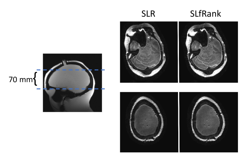
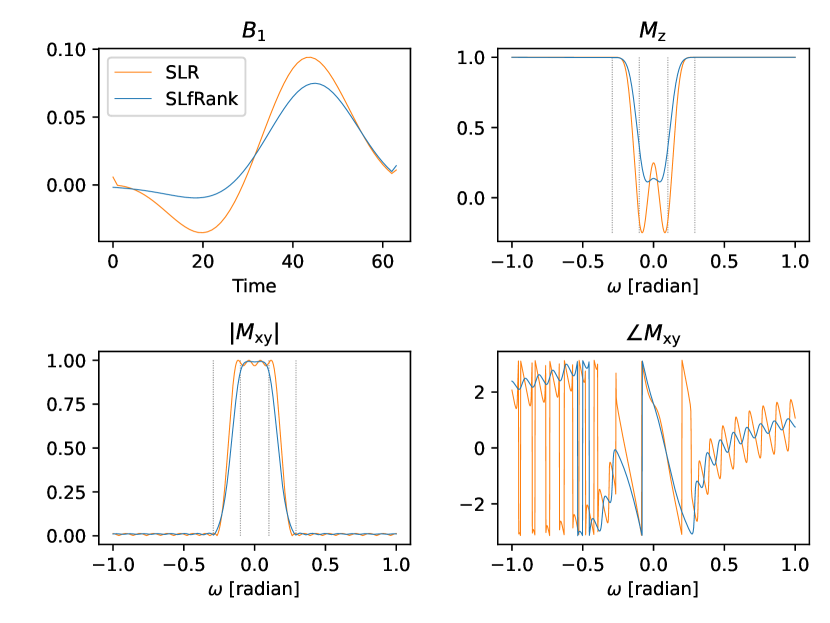
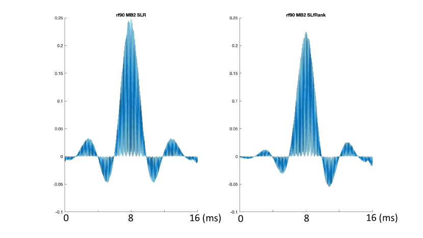
Another way of looking at the convex relaxation is that we relax the constraint that 𝐗𝐗\mathbf{X} is a rank-1 matrix to that 𝐗𝐗\mathbf{X} being a positive semi-definite matrix. Such relaxation has been applied in many other applications, such as max-cut [21], matrix completion [22], and phase retrieval [23]. ; a,b,P; (1a∗b∗aPaaPabbPbaPbb); (The following constraint is for spin-echo refocusing); Note that an,0subscript𝑎𝑛0a_{n,0} and bn,0subscript𝑏𝑛0b_{n,0} are the first elements of 𝐚𝐚\mathbf{a} and 𝐛𝐛\mathbf{b} respectively and 𝐏aa,𝐏ba,𝐏ab,𝐏bbsubscript𝐏𝑎𝑎subscript𝐏𝑏𝑎subscript𝐏𝑎𝑏subscript𝐏𝑏𝑏\mathbf{P}_{aa},\mathbf{P}_{ba},\mathbf{P}_{ab},\mathbf{P}_{bb} are submatrices of 𝐏𝐏\mathbf{P}.; Also the constraints on 𝐛𝐛\mathbf{b} are only imposed for spin-echo refocusing.; Table 1 and 2 contain the δ𝛿\delta parameters used for different pulse types. For bands that are not specified, the δ𝛿\delta parameters are set to 1 and the desired profiles are set to 0. ; We have included a proof sketch in the Supplementary Materials for completeness.; Once we obtain CK polynomial coefficients 𝐚𝐚\mathbf{a} and 𝐛𝐛\mathbf{b}, we can then use the inverse SLR transform in Section 2.3 to recover the hard pulses 𝐁1,1,,𝐁1,nsubscript𝐁11subscript𝐁1𝑛\mathbf{B}_{1,1},\ldots,\mathbf{B}_{1,n}.; We follow [11] to choose the same ripple, passband, stopband and transition width parameters for both SLR and SLfRank.; We have also generated more comparisons in the Supplementary Materials with TBW=4 and 10, along with n=100𝑛100n=100.; gradient; , with band boundaries denoted by dotted gray lines; gradient; gradient; , with band boundaries denoted by dotted gray lines; gradient; , with band boundaries denoted by dotted gray lines; , with band boundaries denoted by dotted gray lines; , with band boundaries denoted by dotted gray lines; , with band boundaries denoted by dotted gray lines; , with band boundaries denoted by dotted gray lines; , with band boundaries denoted by dotted gray lines; , with band boundaries denoted by dotted gray lines; , with band boundaries denoted by dotted gray lines; Excitation slice profile using the linear phase excitation pulse generated from SLR and SLfRank, respectively. The measured slice profile matches well with the numerical simulation result. The phase response of SLfRank pulse is more linear than SLR.; Excitation slice profile using the linear phase excitation pulse generated from SLR and SLfRank, respectively. The measured slice profile matches well with the numerical simulation result. The phase response of SLfRank pulse is more linear than SLR.; To demonstrate the technical feasibility of the proposed algorithm, we performed a phantom experiment to measure the slice profile of a linear phase excitation pulse designed using both SLR and SLfRank. We also compared it with numerical results. The experiment was performed on a GE 3T scanner with a 32-channel head coil, using a custom-built GRE sequence by changing the frequency-encoding gradient to slice-selection direction. As shown in Figure 9, the measured slice profiles matched well with the numerical experiment. Note that the phase profile of SLfRank pulse is flatter than that of SLR pulse. ; The multi-band excitation pulses (MB factor = 2) designed using SLR and SLfRank, respectively. The energy of the two pulses is 0.142 and 0.115, respectively, indicating a 19% reduction of the RF energy.; The multi-band excitation pulses (MB factor = 2) designed using SLR and SLfRank, respectively. The energy of the two pulses is 0.142 and 0.115, respectively, indicating a 19% reduction of the RF energy.; Brain water phantom images acquired using the MB pulses in Figure 10. The two slices were simultaneously excited with 70 cm apart.; Brain water phantom images acquired using the MB pulses in Figure 10. The two slices were simultaneously excited with 70 cm apart.; To further demonstrate its application, we implemented multi-band RF pulse (Figure  10) and tested it on a brain water phantom (Figure  11). Specifically, the RF pulse was designed with a multi-band factor of 2, slice thickness of 2 mm and 70 mm apart. The RF pulse length was 16 ms, which was then incorporated into a spin-echo EPI sequence. Key parameters of the acquisition were: TR = 4000 ms, TE = 72.7 ms, FOV = 220 * 220 mm, matrix = 110*110, slice thickness = 2mm, slice gap = 0, number of slice = 35. The acquired data was reconstructed using SENSE with the sensitivity map acquired from a separate low-resolution GRE sequence. Compared with the conventional SLR pulse, SLfRank has a reduction of 19% energy with similar image quality.; be; Note that peak amplitude reduction is not guaranteed in all cases. In Supplementary Materials, we see that peak RF amplitude can increase for saturation pulses when designed with SLfRank.; The main reason SLfRank has lower energy than SLR is that it jointly minimizes the energy as the objective for both CK polynomials. The optimal design for a single polynomial in SLR is an equi-ripple filter (such as using Remez), which oscillates and touches the upper and lower constraint boundaries. SLfRank, on the other hand, does not have to be equi-ripple. And the results show that the minimum energy pulse profile usually touches the constraint boundaries near the edges, and then stays along one side without oscillating. This allows SLfRank to satisfy the profile constraints with lower energy. Note that SLfRank directly imposes time band-width and the desired magnetization profile constraints in the design. Therefore, the resulting pulse must satisfy the specified parameters. ; In particular, the current SLfRank algorithm can readily be used for quadratic phase and multiband designs, as we only need to specify desired magnetization profiles and appropriate constraints. Root flipping can potentially be a direction to explore, where we further reduce peak RF amplitude. In particular, we could apply root flipping on one of the CK polynomials after obtaining them from SLfRank. In general, we believe SLfRank could be a drop-in replacement for SLR in most applications.; To accelerate the convergence of the iterative algorithm, we can potentially use SLR pulses to initialize the convex program. We can also explore a multi-level design where we use SLfRank CK polynomials discretized on a coarser resolution for initialization. For example, we can first solve the problem for n=16𝑛16n=16 and up-interpolate the result to n=64𝑛64n=64 as initialization.; In particular, the SLR transform assumes the initial CK parameters to be α0=1subscript𝛼01\alpha_{0}=1 and β0=0subscript𝛽00\beta_{0}=0. With arbitrary α0subscript𝛼0\alpha_{0} and β0subscript𝛽0\beta_{0}, let us define the resulting CK parameters after the n𝑛nth hard pulse to be α~nsubscript~𝛼𝑛\tilde{\alpha}_{n} and β~nsubscript~𝛽𝑛\tilde{\beta}_{n}, then they are related to the original CK parameters with equilibrium as starting point as:
(α~nβ~n)=(αnβnβnαn)(100z1)(α0β0).matrixsubscript~𝛼𝑛subscript~𝛽𝑛matrixsubscript𝛼𝑛superscriptsubscript𝛽𝑛subscript𝛽𝑛subscript𝛼𝑛matrix100superscript𝑧1matrixsubscript𝛼0subscript𝛽0\displaystyle\begin{pmatrix}\tilde{\alpha}_{n}\\ \tilde{\beta}_{n}\end{pmatrix}=\begin{pmatrix}\alpha_{n}&-\beta_{n}^{*}\\ \beta_{n}&\alpha_{n}\end{pmatrix}\begin{pmatrix}1&0\\ 0&z^{-1}\end{pmatrix}\begin{pmatrix}\alpha_{0}\\ \beta_{0}\end{pmatrix}.
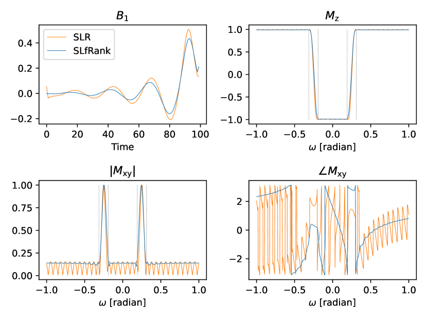
To generalize to arbitrary starting point, the transform or the design process should be changed accordingly to form a complete SLR algorithm. ; Here we compare SLR and SLfRank pulses with time bandwidth (TBW) = 4 and n=64𝑛64n=64.; Here we compare SLR and SLfRank pulses with TBW = 10 and n=64𝑛64n=64.; Here we compare SLR and SLfRank pulses with TBW = 8 and n=100𝑛100n=100.)
Abstract

The Shinnar-Le-Roux (SLR) algorithm is widely used to design frequency selective pulses with large flip angles. We improve its design process to generate pulses with lower energy (by as much as 26%) and more accurate phase profiles.

Concretely, the SLR algorithm consists of two steps: (1) an invertible transform between frequency selective pulses and polynomial pairs that represent Cayley-Klein (CK) parameters and (2) the design of the CK polynomial pair to match the desired magnetization profiles. Because the CK polynomial pair is bi-linearly coupled, the original algorithm sequentially solves for each polynomial instead of jointly. This results in sub-optimal pulses.

Instead, we leverage a convex relaxation technique, commonly used for low rank matrix recovery, to address the bi-linearity. Our numerical experiments show that the resulting pulses are almost always globally optimal in practice. For slice excitation, the proposed algorithm results in more accurate linear phase profiles. And in general the improved pulses have lower energy than the original SLR pulses.

{IEEEkeywords}

MRI, RF Pulse Design, Shinnar-Le-Roux Algorithm, Convex Relaxation, Low Rank Matrix

1 Introduction

Frequency selective radio-frequency (RF) pulses are essential components in magnetic resonance imaging (MRI). Among other functions, they are used for spectral saturation, inversion, and spin-echo refocusing. Several accelerated imaging techniques, such as simultaneous multi-slice imaging, further build on advances in RF pulse design . Improvements in frequency selective pulse design can therefore benefit many applications .

The Shinnar-Le-Roux (SLR) algorithm [3, 4, 5, 6, 7, 8, 9, 10, 11] is widely used to design frequency selective pulses with large flip angles. It vastly simplifies the highly non-linear pulse design problem by mapping RF pulses to pairs of polynomial that represent Cayley-Klein (CK) parameters. Pulse designers can then solve for polynomial pairs using filter design algorithms and convert them back. Users can also incorporate pulse energy as a design objective, which is crucial when the specific absorption rate (SAR) is a limiting factor.

However, there is a subtle issue in the current SLR design process: the algorithm does not jointly design the CK polynomial pair. This can lead to sub-optimal pulses with higher energy and inaccurate phase profiles.

The main challenge preventing joint recovery is that CK parameters are bi-linearly coupled. For example, the transverse magnetization Mxysubscript𝑀xyM_{\mathrm{xy}} is related to the CK parameters, α𝛼\alpha and β𝛽\beta, as Mxy=2αβsubscript𝑀xy2superscript𝛼𝛽M_{\mathrm{xy}}=2\alpha^{*}\beta. To bypass the bi-linear coupling, the SLR algorithm first converts constraints on Mxysubscript𝑀xyM_{\mathrm{xy}} to constraints on β𝛽\beta. It then finds a β𝛽\beta to satisfy the constraints and solves for an α𝛼\alpha to minimize pulse energy. The conversion between constraints on magnetization profiles and on β𝛽\beta is not exact. SLR pulses can produce different phase profiles than the desired ones because the design does not account for the phase of α𝛼\alpha. Such process also does not recover the β𝛽\beta that minimizes energy.

Refer to caption
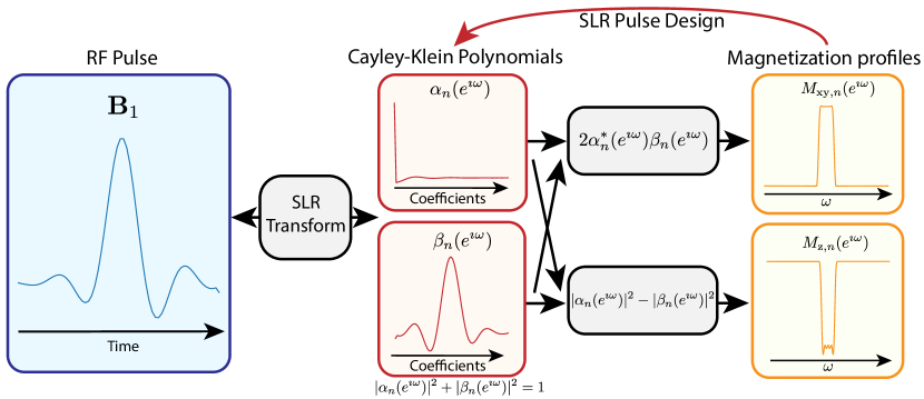
Figure 1: An overview of the SLR algorithm, which consists of two steps: (1) an invertible transform between frequency selective pulses and polynomial pairs that represent Cayley-Klein (CK) parameters and (2) the design of the CK polynomial pair to match a desired magnetization profile. Because the CK polynomial pair is bi-linearly coupled, the original algorithm sequentially solves for each polynomial instead of jointly. This results in sub-optimal pulses. Instead, we propose an improved SLR (SLfRank) design process that can jointly solve for the CK polynomial pair. The new design can specify constraints directly on magnetization profiles, and optimize both CK polynomials to minimize pulse energy. In particular, we leverage a convex relaxation technique, commonly used for low rank matrix recovery, to address the bi-linearity.

To correct phase profile errors in the SLR algorithm, Barral et al. [12] proposed a heuristic to alternatively solve for CK parameters. While effective, the method does not jointly optimize the CK polynomials to minimize pulse energy. Besides the SLR algorithm, other pulse design methods present different tradeoffs. A line of work using the inverse scattering transform [13, 14, 15, 16, 17, 18, 19] can specify constraints on magnetization profiles and minimize pulse energy. But the resulting pulses have infinite lengths. Optimal control (OC) methods [20] have also been extensively used for pulse design.

In particular, we propose an improved SLR design process to jointly solve for the CK polynomial pair. The new design can specify constraints directly on magnetization profiles, and optimize both CK polynomials to minimize pulse energy. We leverage a convex relaxation technique, commonly used for low rank matrix recovery [21, 22, 23], to address the bi-linearity. Although we relax the problem, the convex program allows us to check for optimality. And our numerical experiments show that the resulting pulses almost always attain the global solution in practice. Because the algorithm is based on rank factorization, we name the proposed algorithm SLfRank.

Following [11], we use SLfRank to design pulses for excitation, inversion, saturation, and spin-echo refocusing. For slice excitation, the pulses result in more accurate linear phase profiles. And in general they have lower energy than the original SLR pulses by as much as 26%percent2626\%.

2 Overview of the SLR algorithm

Here we give an overview of the original SLR algorithm, which consists of two steps: (1) an invertible transform between frequency selective pulses and polynomial pairs that represent CK parameters and (2) the design of the CK polynomial pair to match a desired magnetization profile.

Our work only improves the design aspect, but we describe the transform as well for completeness. We also highlight its use of quaternion representations, which provides insight into the proposed convex program.

We assume our readers are familiar with the classical Bloch equation in vector representation, but not necessarily in other forms. Therefore, we first give an introduction to the different representations used in the SLR algorithm.

2.1 Vectors to Quaternions to Cayley-Klein Parameters
Refer to caption
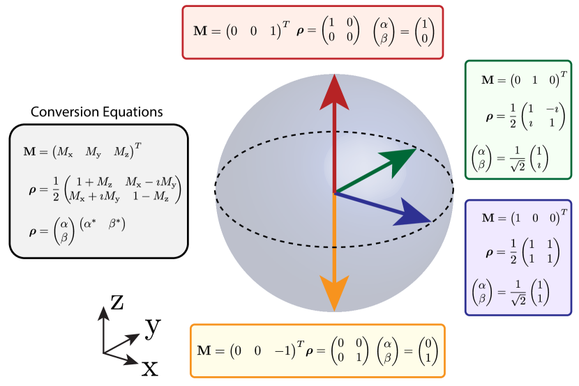
Figure 2: Illustration of different representations: magnetization vector 𝐌𝐌\mathbf{M}, quaternion 𝝆𝝆\bm{\rho}, and Cayley-Klein (CK) parameters α𝛼\alpha and β𝛽\beta. We can map vectors to quaternions using an orthogonal matrix basis formed by the Pauli matrices and the identity matrix. CK parameters are simply rank-one factors of quaternions. This shows the bi-linear relationship between magnetization vectors and CK parameters.

We begin by going over the relationship between magnetization vectors and CK parameters. We use the quaternion as an intermediate representation, which allows us to map vectors to quaternions, and then to CK parameters. This path exposes the bi-linear relationship between vectors and CK parameters, which we focus on in later sections. Figure 2 provides illustrative examples of different representations.

Concretely, let us define the following matrices:

𝐈=(1001)𝐈matrix1001\displaystyle\mathbf{I}=\begin{pmatrix}1&0\\ 0&1\end{pmatrix} 𝝈x=(0110)subscript𝝈xmatrix0110\displaystyle\bm{\sigma}_{\mathrm{x}}=\begin{pmatrix}0&1\\ 1&0\end{pmatrix}
𝝈y=(0ii0)subscript𝝈ymatrix0𝑖𝑖0\displaystyle\bm{\sigma}_{\mathrm{y}}=\begin{pmatrix}0&-i\\ i&0\end{pmatrix} 𝝈z=(1001)subscript𝝈zmatrix1001\displaystyle\bm{\sigma}_{\mathrm{z}}=\begin{pmatrix}1&0\\ 0&-1\end{pmatrix}

where i=1𝑖1i=\sqrt{-1}. The matrices 𝝈xsubscript𝝈x\bm{\sigma}_{\mathrm{x}}, 𝝈ysubscript𝝈y\bm{\sigma}_{\mathrm{y}}, and 𝝈zsubscript𝝈z\bm{\sigma}_{\mathrm{z}} are often called the Pauli matrices. Together with the identity matrix 𝐈𝐈\mathbf{I}, they form an orthogonal basis for 2-by-2 Hermitian matrices.

Then, for any magnetization vector 𝐌=(MxMyMz)T𝐌superscriptmatrixsubscript𝑀xsubscript𝑀ysubscript𝑀z𝑇\mathbf{M}=\begin{pmatrix}M_{\mathrm{x}}&M_{\mathrm{y}}&M_{\mathrm{z}}\end{pmatrix}^{T}, we can convert it to a quaternion 𝝆𝝆\bm{\rho} as

𝝆𝝆\displaystyle\bm{\rho} =12(𝐈+Mx𝝈x+My𝝈y+Mz𝝈z)absent12𝐈subscript𝑀xsubscript𝝈xsubscript𝑀ysubscript𝝈ysubscript𝑀zsubscript𝝈z\displaystyle=\frac{1}{2}(\mathbf{I}+M_{\mathrm{x}}\bm{\sigma}_{\mathrm{x}}+M_{\mathrm{y}}\bm{\sigma}_{\mathrm{y}}+M_{\mathrm{z}}\bm{\sigma}_{\mathrm{z}}) (1)
=12(1+MzMxiMyMx+iMy1Mz).absent12matrix1subscript𝑀zsubscript𝑀x𝑖subscript𝑀ysubscript𝑀x𝑖subscript𝑀y1subscript𝑀z\displaystyle=\frac{1}{2}\begin{pmatrix}1+M_{\mathrm{z}}&M_{\mathrm{x}}-iM_{\mathrm{y}}\\ M_{\mathrm{x}}+iM_{\mathrm{y}}&1-M_{\mathrm{z}}\end{pmatrix}. (2)

Note that the trace of 𝝆𝝆\bm{\rho} is one by construction.

Quaternions can be seen as extensions of complex numbers, with the Pauli matrices acting like the imaginary number. And just as complex numbers can easily represent two-dimensional rotations, quaternions can compactly describe three-dimensional rotations.

In particular, if we want to rotate a quaternion 𝝆𝝆\bm{\rho} around an unit-norm axis 𝐮=(uxuyuz)T𝐮superscriptmatrixsubscript𝑢xsubscript𝑢ysubscript𝑢z𝑇\mathbf{u}=\begin{pmatrix}u_{\mathrm{x}}&u_{\mathrm{y}}&u_{\mathrm{z}}\end{pmatrix}^{T} by angle θ𝜃\theta, then defining 𝐮𝝈=ux𝝈x+uy𝝈y+uz𝝈z𝐮𝝈subscript𝑢xsubscript𝝈xsubscript𝑢ysubscript𝝈ysubscript𝑢zsubscript𝝈z\mathbf{u}\cdot\bm{\sigma}=u_{\mathrm{x}}\bm{\sigma}_{\mathrm{x}}+u_{\mathrm{y}}\bm{\sigma}_{\mathrm{y}}+u_{\mathrm{z}}\bm{\sigma}_{\mathrm{z}}, the rotated quaternion θ𝐮(𝝆)subscript𝜃𝐮𝝆\mathcal{R}_{\theta\mathbf{u}}(\bm{\rho}) can be expressed as

θ𝐮(𝝆)=eiθ(𝐮𝝈)/2𝝆eiθ(𝐮𝝈)/2,subscript𝜃𝐮𝝆superscript𝑒𝑖𝜃𝐮𝝈2𝝆superscript𝑒𝑖𝜃𝐮𝝈2\displaystyle\mathcal{R}_{\theta\mathbf{u}}(\bm{\rho})=e^{i\theta(\mathbf{u}\cdot\bm{\sigma})/2}\bm{\rho}e^{-i\theta(\mathbf{u}\cdot\bm{\sigma})/2}, (3)

where the exponential is a matrix exponential given by

eiθ(𝐮𝝈)/2=𝐈cos(θ/2)+i(𝐮𝝈)sin(θ/2).superscript𝑒𝑖𝜃𝐮𝝈2𝐈𝜃2𝑖𝐮𝝈𝜃2e^{i\theta(\mathbf{u}\cdot\bm{\sigma})/2}=\mathbf{I}\cos(\theta/2)+i(\mathbf{u}\cdot\bm{\sigma})\sin(\theta/2).

This simple rotation representation makes quaternions ideal for describing spin dynamics.

Another useful property of quaternions is that the rank of a quaternion is related to the norm of the equivalent magnetization vector. A quaternion 𝝆𝝆\bm{\rho} is always positive semi-definite as long as its vector representation 𝐌𝐌\mathbf{M} has a norm less than one. That is,

𝝆0|Mx|2+|My|2+|Mz|21.succeeds-or-equals𝝆0superscriptsubscript𝑀x2superscriptsubscript𝑀y2superscriptsubscript𝑀z21\bm{\rho}\succeq 0\Leftrightarrow|M_{\mathrm{x}}|^{2}+|M_{\mathrm{y}}|^{2}+|M_{\mathrm{z}}|^{2}\leq 1.

This can be seen from the Schur complement of 𝝆𝝆\bm{\rho}, [1Mz|Mxy|2/(1+Mz)]/2delimited-[]1subscript𝑀zsuperscriptsubscript𝑀xy21subscript𝑀z2[1-M_{\mathrm{z}}-|M_{\mathrm{xy}}|^{2}/(1+M_{\mathrm{z}})]/2, which is non-negative if and only if 𝝆𝝆\bm{\rho} is positive semi-definite.

Moreover, if the vector representation has a unit norm, then the Schur complement is zero. This implies that the quaternion is rank deficient. Because the trace of the quaternion is one by construction, the rank can only be one. Therefore, we obtain

𝝆=(αβ)(αβ)|Mx|2+|My|2+|Mz|2=1,𝝆matrix𝛼𝛽matrixsuperscript𝛼superscript𝛽superscriptsubscript𝑀x2superscriptsubscript𝑀y2superscriptsubscript𝑀z21\displaystyle\bm{\rho}=\begin{pmatrix}\alpha\\ \beta\end{pmatrix}\begin{array}[]{@{}c@{}}\begin{pmatrix}\alpha^{*}&\beta^{*}\end{pmatrix}\\ \mathstrut\end{array}\Leftrightarrow|M_{\mathrm{x}}|^{2}+|M_{\mathrm{y}}|^{2}+|M_{\mathrm{z}}|^{2}=1, (6)

for some α𝛼\alpha\in\mathbb{C} and β𝛽\beta\in\mathbb{C} such that |α|2+|β|2=1superscript𝛼2superscript𝛽21|\alpha|^{2}+|\beta|^{2}=1.

The parameters α𝛼\alpha and β𝛽\beta are often called the Cayley-Klein (CK) parameters. Because rotation operators in Eq. (3) preserve the quaternion rank, CK parameters can always represent magnetization in the absence of relaxation effects. Note also that the energy of CK parameters must sum to one. That is,

αα+ββ=1.𝛼superscript𝛼𝛽superscript𝛽1\alpha\alpha^{*}+\beta\beta^{*}=1.

To convert between CK parameters and magnetization vectors, we simply match equations (2) and (6), and obtain

Mxy=2βαandMz=ααββ,subscript𝑀xy2𝛽superscript𝛼andsubscript𝑀z𝛼superscript𝛼𝛽superscript𝛽\displaystyle M_{\mathrm{xy}}=2\beta\alpha^{*}~{}\text{and}~{}M_{\mathrm{z}}=\alpha\alpha^{*}-\beta\beta^{*},

which explicitly shows the bi-linear relationship between CK parameters and magnetization vectors.

In summary, we can convert vectors to quaternions using the Pauli matrices. CK parameters are then factors of quaternions when energy is conserved.

2.2 Forward SLR Transform
Refer to caption
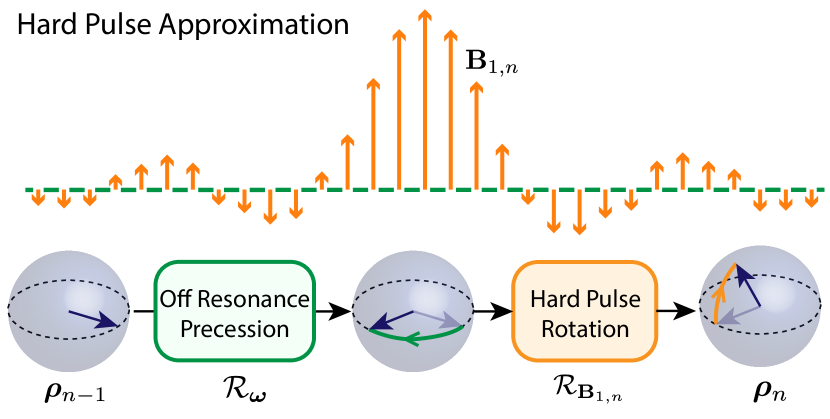
Figure 3: The SLR algorithm considers the hard pulse approximation, which discretizes the RF pulse to a sequence of impulses, also known as hard pulses. The magnetization evolution can then described as a recursion of off-resonance precession followed by hard pulse rotation. Off-resonance rotates magnetization around the z-axis. And a hard pulse rotates magnetization around an axis in the transverse plane.

With the quaternion and CK parameter representations, we can obtain the forward SLR transform by going through a discretized version of the Bloch equation. In particular, the forward SLR transform converts any RF pulse to two polynomials that represent CK parameters.

To do so, the forward SLR transform first considers the hard pulse approximation, which discretizes the RF pulse to a sequence of impulses, also known as hard pulses. The magnetization evolution then becomes a recursion of off-resonance precession followed by hard pulse rotation. Off-resonance rotates magnetization around the z-axis. And a hard pulse rotates magnetization around an axis in the transverse plane. Figure 3 provides an illustration.

Concretely, let 𝝎=(00ω)T𝝎superscriptmatrix00𝜔𝑇\bm{\omega}=\begin{pmatrix}0&0&\omega\end{pmatrix}^{T} represent off-resonance with frequency ω𝜔\omega in radian and 𝐁1,n=(B1,x,nB1,y,n0)Tsubscript𝐁1𝑛superscriptmatrixsubscript𝐵1x𝑛subscript𝐵1y𝑛0𝑇\mathbf{B}_{1,n}=\begin{pmatrix}B_{1,\mathrm{x},n}&B_{1,\mathrm{y},n}&0\end{pmatrix}^{T} represent the n𝑛nth hard pulse in radian, then the quaternion after the n𝑛nth hard pulse is given by

𝝆n=𝐁1,n(𝝎(𝝆n1)).subscript𝝆𝑛subscriptsubscript𝐁1𝑛subscript𝝎subscript𝝆𝑛1\displaystyle\bm{\rho}_{n}=\mathcal{R}_{\mathbf{B}_{1,n}}(\mathcal{R}_{\bm{\omega}}(\bm{\rho}_{n-1})). (7)

Using equation (3), we obtain the following expressions for the rotation operators:

𝐁1,n(𝝆)=(cnsnsncn)𝝆(cnsnsncn)subscriptsubscript𝐁1𝑛𝝆matrixsubscript𝑐𝑛superscriptsubscript𝑠𝑛subscript𝑠𝑛subscript𝑐𝑛𝝆matrixsubscript𝑐𝑛superscriptsubscript𝑠𝑛subscript𝑠𝑛subscript𝑐𝑛\mathcal{R}_{\mathbf{B}_{1,n}}(\bm{\rho})=\begin{pmatrix}c_{n}&-s_{n}^{*}\\ s_{n}&c_{n}\end{pmatrix}\bm{\rho}\begin{pmatrix}c_{n}&s_{n}^{*}\\ -s_{n}&c_{n}\end{pmatrix}
𝝎(𝝆)=(100z1)𝝆(100z)subscript𝝎𝝆matrix100superscript𝑧1𝝆matrix100𝑧\mathcal{R}_{\bm{\omega}}(\bm{\rho})=\begin{pmatrix}1&0\\ 0&z^{-1}\end{pmatrix}\bm{\rho}\begin{pmatrix}1&0\\ 0&z\end{pmatrix}

where

cnsubscript𝑐𝑛\displaystyle c_{n} =cos(𝐁1,n/2),absentnormsubscript𝐁1𝑛2\displaystyle=\cos(\|\mathbf{B}_{1,n}\|/2),
snsubscript𝑠𝑛\displaystyle s_{n} =i(B1,x,n+iB1,y,n)𝐁1,nsin(𝐁1,n/2),absent𝑖subscript𝐵1x𝑛𝑖subscript𝐵1y𝑛normsubscript𝐁1𝑛normsubscript𝐁1𝑛2\displaystyle=\frac{i(B_{1,\mathrm{x},n}+iB_{1,\mathrm{y},n})}{\|\mathbf{B}_{1,n}\|}\sin(\|\mathbf{B}_{1,n}\|/2),
z𝑧\displaystyle z =eiω.absentsuperscript𝑒𝑖𝜔\displaystyle=e^{i\omega}.

We can further simplify the forward evolution by using CK parameters as representations. Substituting the rotation operators and using equation (6), we have

(αnβn)=(cnsnsncn)(100z1)(αn1βn1).matrixsubscript𝛼𝑛subscript𝛽𝑛matrixsubscript𝑐𝑛superscriptsubscript𝑠𝑛subscript𝑠𝑛subscript𝑐𝑛matrix100superscript𝑧1matrixsubscript𝛼𝑛1subscript𝛽𝑛1\displaystyle\begin{pmatrix}\alpha_{n}\\ \beta_{n}\end{pmatrix}=\begin{pmatrix}c_{n}&-s_{n}^{*}\\ s_{n}&c_{n}\end{pmatrix}\begin{pmatrix}1&0\\ 0&z^{-1}\end{pmatrix}\begin{pmatrix}\alpha_{n-1}\\ \beta_{n-1}\end{pmatrix}. (8)

In each time step, the CK parameters gain one additional z𝑧z factor. Therefore, starting from an initial CK parameter α0=1subscript𝛼01\alpha_{0}=1 and β0=0subscript𝛽00\beta_{0}=0 at equilibrium, the CK parameters after the n𝑛nth hard pulse become degree-(n1)𝑛1(n-1) polynomials in z𝑧z. That is

αn(z)subscript𝛼𝑛𝑧\displaystyle\alpha_{n}(z) =j=0n1an,jzj,absentsuperscriptsubscript𝑗0𝑛1subscript𝑎𝑛𝑗superscript𝑧𝑗\displaystyle=\sum_{j=0}^{n-1}a_{n,j}z^{-j}, (9)
βn(z)subscript𝛽𝑛𝑧\displaystyle\beta_{n}(z) =j=0n1bn,jzj.absentsuperscriptsubscript𝑗0𝑛1subscript𝑏𝑛𝑗superscript𝑧𝑗\displaystyle=\sum_{j=0}^{n-1}b_{n,j}z^{-j}.

Note that the energy of the CK parameters is preserved for all n𝑛n. That is,

αn(z)αn(z)+βn(z)βn(z)subscript𝛼𝑛𝑧superscriptsubscript𝛼𝑛𝑧subscript𝛽𝑛𝑧superscriptsubscript𝛽𝑛𝑧\displaystyle\alpha_{n}(z)\alpha_{n}^{*}(z)+\beta_{n}(z)\beta_{n}^{*}(z) =1.absent1\displaystyle=1. (10)

And we can easily obtain magnetization vectors after the n𝑛nth hard pulse as:

Mxy,n(z)subscript𝑀xy𝑛𝑧\displaystyle M_{\mathrm{xy},n}(z) =2βn(z)αn(z)absent2subscript𝛽𝑛𝑧superscriptsubscript𝛼𝑛𝑧\displaystyle=2\beta_{n}(z)\alpha_{n}^{*}(z) (11)
Mz,n(z)subscript𝑀z𝑛𝑧\displaystyle M_{\mathrm{z},n}(z) =αn(z)αn(z)βn(z)βn(z),absentsubscript𝛼𝑛𝑧superscriptsubscript𝛼𝑛𝑧subscript𝛽𝑛𝑧superscriptsubscript𝛽𝑛𝑧\displaystyle=\alpha_{n}(z)\alpha_{n}^{*}(z)-\beta_{n}(z)\beta_{n}^{*}(z),

In summary, under the hard pulse approximation, the forward SLR transform can convert any RF pulse to two polynomials that represent the CK parameters, as shown in Eq. (9). The polynomials must also satisfy an energy constraint in Eq. (10). What is remarkable is that given two polynomials with the energy constraint, we can always convert them back to a valid pulse with the inverse SLR transform.

2.3 Inverse SLR Transform

Given any polynomial pair that satisfies the energy constraint in Eq. (10), the inverse SLR transform can map it back to an RF pulse. It does so by considering the following backward recursion of Eq. (8):

(αn1βn1)matrixsubscript𝛼𝑛1subscript𝛽𝑛1\displaystyle\begin{pmatrix}\alpha_{n-1}\\ \beta_{n-1}\end{pmatrix} =(100z)(cnsnsncn)(αnβn).absentmatrix100𝑧matrixsubscript𝑐𝑛superscriptsubscript𝑠𝑛subscript𝑠𝑛subscript𝑐𝑛matrixsubscript𝛼𝑛subscript𝛽𝑛\displaystyle=\begin{pmatrix}1&0\\ 0&z\end{pmatrix}\begin{pmatrix}c_{n}&s_{n}^{*}\\ -s_{n}&c_{n}\end{pmatrix}\begin{pmatrix}\alpha_{n}\\ \beta_{n}\end{pmatrix}.

It then recovers cnsubscript𝑐𝑛c_{n} and snsubscript𝑠𝑛s_{n} such that αn1subscript𝛼𝑛1\alpha_{n-1} and βn1subscript𝛽𝑛1\beta_{n-1} represent valid CK parameters.

For αn1subscript𝛼𝑛1\alpha_{n-1} and βn1subscript𝛽𝑛1\beta_{n-1} to be valid, they need to be degree-(n2)𝑛2(n-2) polynomials and satisfy the energy constraint. Note that as long as |cn|2+|sn|2=1superscriptsubscript𝑐𝑛2superscriptsubscript𝑠𝑛21|c_{n}|^{2}+|s_{n}|^{2}=1, the energy constraint is satisfied. To ensure αn1subscript𝛼𝑛1\alpha_{n-1} and βn1subscript𝛽𝑛1\beta_{n-1} are degree-(n2)𝑛2(n-2) polynomials, we need

snan,0+cnbn,0subscript𝑠𝑛subscript𝑎𝑛0subscript𝑐𝑛subscript𝑏𝑛0\displaystyle-s_{n}a_{n,0}+c_{n}b_{n,0} =0absent0\displaystyle=0 (12)
cnan,n1+snbn,n1subscript𝑐𝑛subscript𝑎𝑛𝑛1superscriptsubscript𝑠𝑛subscript𝑏𝑛𝑛1\displaystyle c_{n}a_{n,n-1}+s_{n}^{*}b_{n,n-1} =0,absent0\displaystyle=0, (13)

which allow us to solve for two sets of solutions for cnsubscript𝑐𝑛c_{n} and snsubscript𝑠𝑛s_{n}.

It turns out these two solutions are the same because the energy constraint in Eq. (10) implies

an,n1an,0+bn,n1bn,0=0,subscript𝑎𝑛𝑛1subscriptsuperscript𝑎𝑛0subscript𝑏𝑛𝑛1subscriptsuperscript𝑏𝑛00a_{n,n-1}a^{*}_{n,0}+b_{n,n-1}b^{*}_{n,0}=0,

where the left hand side is the leading coefficient of the polynomial αn(z)αn(z)+βn(z)βn(z)subscript𝛼𝑛𝑧superscriptsubscript𝛼𝑛𝑧subscript𝛽𝑛𝑧superscriptsubscript𝛽𝑛𝑧\alpha_{n}(z)\alpha_{n}^{*}(z)+\beta_{n}(z)\beta_{n}^{*}(z).

Therefore, we can recover the parameters as:

cnsubscript𝑐𝑛\displaystyle c_{n} =an,0|an,0|2+|bn,0|2=bn,n1|an,n1|2+|bn,n1|2absentsubscript𝑎𝑛0superscriptsubscript𝑎𝑛02superscriptsubscript𝑏𝑛02subscript𝑏𝑛𝑛1superscriptsubscript𝑎𝑛𝑛12superscriptsubscript𝑏𝑛𝑛12\displaystyle=\frac{a_{n,0}}{\sqrt{|a_{n,0}|^{2}+|b_{n,0}|^{2}}}=\frac{b_{n,n-1}}{\sqrt{|a_{n,n-1}|^{2}+|b_{n,n-1}|^{2}}}
snsubscript𝑠𝑛\displaystyle s_{n} =bn,0|an,0|2+|bn,0|2=an,n1|an,n1|2+|bn,n1|2absentsubscript𝑏𝑛0superscriptsubscript𝑎𝑛02superscriptsubscript𝑏𝑛02superscriptsubscript𝑎𝑛𝑛1superscriptsubscript𝑎𝑛𝑛12superscriptsubscript𝑏𝑛𝑛12\displaystyle=\frac{b_{n,0}}{\sqrt{|a_{n,0}|^{2}+|b_{n,0}|^{2}}}=\frac{-a_{n,n-1}^{*}}{\sqrt{|a_{n,n-1}|^{2}+|b_{n,n-1}|^{2}}}

And we can obtain the n𝑛nth hard pulse as,

ϕnsubscriptitalic-ϕ𝑛\displaystyle\phi_{n} =2arctan(|sn/cn|),absent2arctangentsubscript𝑠𝑛subscript𝑐𝑛\displaystyle=2\arctan(|s_{n}/c_{n}|),
θnsubscript𝜃𝑛\displaystyle\theta_{n} =(ısncn),absentitalic-ısubscript𝑠𝑛superscriptsubscript𝑐𝑛\displaystyle=\angle(-\imath s_{n}c_{n}^{*}),
B1,n,xsubscript𝐵1𝑛x\displaystyle B_{1,n,\mathrm{x}} =ϕncos(θn),absentsubscriptitalic-ϕ𝑛subscript𝜃𝑛\displaystyle=\phi_{n}\cos(\theta_{n}),
B1,n,ysubscript𝐵1𝑛y\displaystyle B_{1,n,\mathrm{y}} =ϕnsin(θn).absentsubscriptitalic-ϕ𝑛subscript𝜃𝑛\displaystyle=\phi_{n}\sin(\theta_{n}).

2.4 Original SLR Design Process

With the SLR transform, the highly non-linear pulse design problem becomes equivalent to designing the CK polynomial pair. The remaining challenge is the bi-linear coupling between αnsubscript𝛼𝑛\alpha_{n} and βnsubscript𝛽𝑛\beta_{n}. The original SLR algorithm bypasses this by sequentially solving for each variable. It first converts design constraints on magnetization profiles to constraints on βnsubscript𝛽𝑛\beta_{n}. Then, it recovers an αnsubscript𝛼𝑛\alpha_{n} that minimizes the pulse energy. In the following, we highlight some advantages and disadvantages of this approach.

There are certain constraints that can be directly expressed in βnsubscript𝛽𝑛\beta_{n}. [11] shows that for spin-echo refocusing pulses, the effective transverse magnetization after crusher gradients can be expressed as

Mxy,n(z)subscript𝑀xy𝑛𝑧\displaystyle M_{\mathrm{xy},n}(z) =βn2(z).absentsuperscriptsubscript𝛽𝑛2𝑧\displaystyle=\beta_{n}^{2}(z).

For single band designs, any constraints on Mxy,nsubscript𝑀xy𝑛M_{\mathrm{xy},n} can then be converted to constraints on βnsubscript𝛽𝑛\beta_{n} up to a global sign change, which does not affect the resulting pulse.

However, for other pulses, we cannot directly translate constraints. Instead, using Eqs. (10) and (11), we only have the following relationships:

|Mxy,n(z)|2superscriptsubscript𝑀xy𝑛𝑧2\displaystyle|M_{\mathrm{xy},n}(z)|^{2} =4|βn(z)|2(1|βn(z)|2),absent4superscriptsubscript𝛽𝑛𝑧21superscriptsubscript𝛽𝑛𝑧2\displaystyle=4|\beta_{n}(z)|^{2}(1-|\beta_{n}(z)|^{2}),
Mz,n(z)subscript𝑀z𝑛𝑧\displaystyle M_{\mathrm{z},n}(z) =12|βn(z)|2.absent12superscriptsubscript𝛽𝑛𝑧2\displaystyle=1-2|\beta_{n}(z)|^{2}.

[11] shows that we can use these equations to specify ripple parameters in min-max filter designs. However, note that we cannot express transverse magnetization phase in terms of βnsubscript𝛽𝑛\beta_{n}.

When the user does not require a particular transverse magnetization phase profile, the original SLR algorithm has more flexibility. One choice is a minimum phase polynomial for βnsubscript𝛽𝑛\beta_{n}. This is equivalent to selecting a βnsubscript𝛽𝑛\beta_{n} polynomial that maximizes its first coefficient Re{bn,0}subscript𝑏𝑛0\Re{b_{n,0}}. Using linear approximation, we can interpret this as maximizing the last hard pulse:

Re{bn,0}=c1cn1snB1,y,n/2.subscript𝑏𝑛0subscript𝑐1subscript𝑐𝑛1subscript𝑠𝑛subscript𝐵1𝑦𝑛2\Re{b_{n,0}}=c_{1}\ldots c_{n-1}s_{n}\approx B_{1,y,n}/2.

However, when the user wants a specific transverse magnetization phase response, such as in slice excitation, the original SLR algorithm cannot find a corresponding βnsubscript𝛽𝑛\beta_{n} polynomial to do so. Instead, it relies on an approximation that αnsubscript𝛼𝑛\alpha_{n} does not contribute much phase and finds a βnsubscript𝛽𝑛\beta_{n} to account for all of the phase of Mxysubscript𝑀xyM_{\mathrm{xy}}. But αnsubscript𝛼𝑛\alpha_{n} always contributes some phase. Therefore, the resulting profile in general deviates from the desired one.

Once we obtain a βnsubscript𝛽𝑛\beta_{n}, the original design process recovers the αnsubscript𝛼𝑛\alpha_{n} polynomial by minimizing pulse energy. In particular, the first polynomial coefficient of αnsubscript𝛼𝑛\alpha_{n} acts as a proxy for pulse energy. Using cj1𝐁1,j2/8subscript𝑐𝑗1superscriptnormsubscript𝐁1𝑗28c_{j}\approx 1-\|\mathbf{B}_{1,j}\|^{2}/8, we have

an,0=c1c2cn118j=1n𝐁1,j2.subscript𝑎𝑛0subscript𝑐1subscript𝑐2subscript𝑐𝑛118superscriptsubscript𝑗1𝑛superscriptnormsubscript𝐁1𝑗2a_{n,0}=c_{1}c_{2}\ldots c_{n}\approx 1-\frac{1}{8}\sum_{j=1}^{n}\|\mathbf{B}_{1,j}\|^{2}.

With fine enough discretization, maximizing an,0subscript𝑎𝑛0a_{n,0} minimizes pulse energy. We can then find the corresponding αnsubscript𝛼𝑛\alpha_{n} by solving for a minimum phase filter.

On the other hand, the βnsubscript𝛽𝑛\beta_{n} polynomial design does not take pulse energy into consideration. It is possible a different βnsubscript𝛽𝑛\beta_{n} that satisfies the constraints results in lower pulse energy. Indeed, our improved SLR design shows that jointly designing αnsubscript𝛼𝑛\alpha_{n} and βnsubscript𝛽𝑛\beta_{n} reduces pulse energy in general.

3 SLfRank: Improved SLR Pulse Design with Rank Factorization

We propose an improved SLR design, named SLfRank, to jointly recover the CK polynomials with a convex program. The new design can specify constraints directly on magnetization profiles, and optimize both CK polynomials to minimize pulse energy. To derive the optimization problem, we first show that all constraints on the CK polynomials can be represented as linear equations on a rank-one matrix. Then we relax matrix rank constraints to positive semi-definite matrix constraints to obtain a convex program.

Concretely let us define the following vectors:

𝝍(z)𝝍𝑧\displaystyle\bm{\psi}(z) =(1zzn1)Tnabsentsuperscriptmatrix1𝑧superscript𝑧𝑛1𝑇superscript𝑛\displaystyle=\begin{pmatrix}1&z&\ldots&z^{n-1}\end{pmatrix}^{T}\in\mathbb{C}^{n}
𝐚𝐚\displaystyle\mathbf{a} =(an,0an,1an,n1)Tnabsentsuperscriptmatrixsubscript𝑎𝑛0subscript𝑎𝑛1subscript𝑎𝑛𝑛1𝑇superscript𝑛\displaystyle=\begin{pmatrix}a_{n,0}&a_{n,1}&\ldots&a_{n,n-1}\end{pmatrix}^{T}\in\mathbb{C}^{n}
𝐛𝐛\displaystyle\mathbf{b} =(bn,0bn,1bn,n1)Tnabsentsuperscriptmatrixsubscript𝑏𝑛0subscript𝑏𝑛1subscript𝑏𝑛𝑛1𝑇superscript𝑛\displaystyle=\begin{pmatrix}b_{n,0}&b_{n,1}&\ldots&b_{n,n-1}\end{pmatrix}^{T}\in\mathbb{C}^{n}

Then the CK polynomials can be expressed as,

αn(z)subscript𝛼𝑛𝑧\displaystyle\alpha_{n}(z) =𝝍(z)𝐚,absentsuperscript𝝍𝑧𝐚\displaystyle=\bm{\psi}^{*}(z)\mathbf{a},
βn(z)subscript𝛽𝑛𝑧\displaystyle\beta_{n}(z) =𝝍(z)𝐛,absentsuperscript𝝍𝑧𝐛\displaystyle=\bm{\psi}^{*}(z)\mathbf{b},

Let us further define 𝐏2n×2n𝐏superscript2𝑛2𝑛\mathbf{P}\in\mathbb{C}^{2n\times 2n} as the outer product of the CK polynomial coefficients :

𝐏=(𝐏aa𝐏ab𝐏ba𝐏bb)=(𝐚𝐛)(𝐚𝐛)𝐏matrixsubscript𝐏𝑎𝑎subscript𝐏𝑎𝑏subscript𝐏𝑏𝑎subscript𝐏𝑏𝑏matrix𝐚𝐛matrixsuperscript𝐚superscript𝐛\mathbf{P}=\begin{pmatrix}\mathbf{P}_{aa}&\mathbf{P}_{ab}\\ \mathbf{P}_{ba}&\mathbf{P}_{bb}\\ \end{pmatrix}=\begin{pmatrix}\mathbf{a}\\ \mathbf{b}\end{pmatrix}\begin{array}[]{@{}c@{}}\begin{pmatrix}\mathbf{a}^{*}&\mathbf{b}^{*}\end{pmatrix}\\ \mathstrut\end{array}

Then, we can express the energy constraint in Eq. (10) and magnetization profiles Eq. (11) in terms of 𝐏𝐏\mathbf{P} as:

11\displaystyle 1 =𝝍(z)(𝐏aa+𝐏bb)𝝍(z)absentsuperscript𝝍𝑧subscript𝐏𝑎𝑎subscript𝐏𝑏𝑏𝝍𝑧\displaystyle=\bm{\psi}^{*}(z)(\mathbf{P}_{aa}+\mathbf{P}_{bb})\bm{\psi}(z)
Mxy,n(z)subscript𝑀xy𝑛𝑧\displaystyle M_{\mathrm{xy},n}(z) =2𝝍(z)𝐏ba𝝍(z)absent2superscript𝝍𝑧subscript𝐏𝑏𝑎𝝍𝑧\displaystyle=2\bm{\psi}^{*}(z)\mathbf{P}_{ba}\bm{\psi}(z)
Mz,n(z)subscript𝑀z𝑛𝑧\displaystyle M_{\mathrm{z},n}(z) =𝝍(z)(𝐏aa𝐏bb)𝝍(z).absentsuperscript𝝍𝑧subscript𝐏𝑎𝑎subscript𝐏𝑏𝑏𝝍𝑧\displaystyle=\bm{\psi}^{*}(z)(\mathbf{P}_{aa}-\mathbf{P}_{bb})\bm{\psi}(z).

The above equations show that we can express all constraints on the CK polynomials as linear equations on a rank-one matrix 𝐏𝐏\mathbf{P}. We can also easily change them to impose inequality constraints on magnetization profiles.

Taking a step back, the matrix 𝐏𝐏\mathbf{P} we have just formed essentially represent the underlying quaternion ρn(z)subscript𝜌𝑛𝑧\rho_{n}(z). In particular, we have

ρn(z)=(𝝍(z)𝟎𝟎𝝍(z))𝐏(𝝍(z)𝟎𝟎𝝍(z))subscript𝜌𝑛𝑧matrixsuperscript𝝍𝑧00superscript𝝍𝑧𝐏matrix𝝍𝑧00𝝍𝑧\rho_{n}(z)=\begin{pmatrix}\bm{\psi}^{*}(z)&\mathbf{0}\\ \mathbf{0}&\bm{\psi}^{*}(z)\\ \end{pmatrix}\mathbf{P}\begin{pmatrix}\bm{\psi}(z)&\mathbf{0}\\ \mathbf{0}&\bm{\psi}(z)\\ \end{pmatrix}

Therefore, one way to interpret the proposed design is that we solve for quaternions instead of CK parameters. And the two representations become equivalent when the quaternion is rank-one.

Optimizing over rank-one matrices is in general non-convex. A common strategy is to relax the rank constraint into a positive semi-definite matrix constraint. Concretely, we can relax the constraint as follows,

𝐏(𝐚𝐛)(𝐚𝐛),succeeds-or-equals𝐏matrix𝐚𝐛matrixsuperscript𝐚superscript𝐛\mathbf{P}\succeq\begin{pmatrix}\mathbf{a}\\ \mathbf{b}\end{pmatrix}\begin{array}[]{@{}c@{}}\begin{pmatrix}\mathbf{a}^{*}&\mathbf{b}^{*}\end{pmatrix}\\ \mathstrut\end{array},

Similar to the original SLR algorithm, we maximize an,0subscript𝑎𝑛0a_{n,0} to minimize pulse energy and bn,0subscript𝑏𝑛0b_{n,0} to generate minimum phase pulses. Putting everything together, we obtain the following optimization problem to design the CK polynomials:

maxabsentmax\displaystyle\underset{}{\text{max}} Re(an,0)+λmpRe(bn,0)subscript𝑎𝑛0subscript𝜆mpsubscript𝑏𝑛0\displaystyle\real(a_{n,0})+\lambda_{\text{mp}}\real(b_{n,0})
s.t. 0,succeeds-or-equalsabsent0\displaystyle\succeq 0,
𝝍(eiω)(𝐏aa+𝐏bb)𝝍(eiω)=1,superscript𝝍superscript𝑒𝑖𝜔subscript𝐏𝑎𝑎subscript𝐏𝑏𝑏𝝍superscript𝑒𝑖𝜔1\displaystyle\bm{\psi}^{*}(e^{i\omega})(\mathbf{P}_{aa}+\mathbf{P}_{bb})\bm{\psi}(e^{i\omega})=1,
|2𝝍(eiω)𝐏ba𝝍(eiω)Mxy,n(eiω)|δxy(eiω),2superscript𝝍superscript𝑒𝑖𝜔subscript𝐏𝑏𝑎𝝍superscript𝑒𝑖𝜔subscript𝑀xy𝑛superscript𝑒𝑖𝜔subscript𝛿xysuperscript𝑒𝑖𝜔\displaystyle|2\bm{\psi}^{*}(e^{i\omega})\mathbf{P}_{ba}\bm{\psi}(e^{i\omega})-M_{\mathrm{xy},n}(e^{i\omega})|\leq\delta_{\mathrm{xy}}(e^{i\omega}),
|𝝍(eiω)(𝐏aa𝐏bb)𝝍(eiω)Mz,n(eiω)|δz(eiω),superscript𝝍superscript𝑒𝑖𝜔subscript𝐏𝑎𝑎subscript𝐏𝑏𝑏𝝍superscript𝑒𝑖𝜔subscript𝑀z𝑛superscript𝑒𝑖𝜔subscript𝛿zsuperscript𝑒𝑖𝜔\displaystyle|\bm{\psi}^{*}(e^{i\omega})(\mathbf{P}_{aa}-\mathbf{P}_{bb})\bm{\psi}(e^{i\omega})-M_{\mathrm{z},n}(e^{i\omega})|\leq\delta_{\mathrm{z}}(e^{i\omega}),
|𝝍(eiω)𝐛βn(eiω)|δβ(eiω),superscript𝝍superscript𝑒𝑖𝜔𝐛subscript𝛽𝑛superscript𝑒𝑖𝜔subscript𝛿𝛽superscript𝑒𝑖𝜔\displaystyle|\bm{\psi}^{*}(e^{i\omega})\mathbf{b}-\beta_{n}(e^{i\omega})|\leq\delta_{\beta}(e^{i\omega}),

where ω𝜔\omega goes from π𝜋-\pi to π𝜋\pi, λmpsubscript𝜆mp\lambda_{\text{mp}} enforces minimum phase conditions, δxysubscript𝛿xy\delta_{\mathrm{xy}}, δzsubscript𝛿z\delta_{\mathrm{z}}, and δβsubscript𝛿𝛽\delta_{\beta} are user-defined error parameters, and Mxy,nsubscript𝑀xy𝑛M_{\mathrm{xy},n} and Mz,nsubscript𝑀z𝑛M_{\mathrm{z},n} represent the desired magnetization profiles.

Table 1: Parameters for excitation, inversion, and saturation pulse designs.
Pass-band with ripple δ1subscript𝛿1\delta_{1} Stop-band with ripple δ2subscript𝛿2\delta_{2}
Pulse (phase) Mxysubscript𝑀xyM_{\mathrm{xy}} δxysubscript𝛿xy\delta_{\mathrm{xy}} Mzsubscript𝑀zM_{\mathrm{z}} δzsubscript𝛿z\delta_{\mathrm{z}} Mxysubscript𝑀xyM_{\mathrm{xy}} δxysubscript𝛿xy\delta_{\mathrm{xy}} Mzsubscript𝑀zM_{\mathrm{z}} δzsubscript𝛿z\delta_{\mathrm{z}}
Excitation (linear) eiω(n+1)/2superscript𝑒𝑖𝜔𝑛12e^{-i\omega(n+1)/2} δ1subscript𝛿1\delta_{1} 0 1(1δ1)21superscript1subscript𝛿12\sqrt{1-(1-\delta_{1})^{2}} 0 δ2subscript𝛿2\delta_{2} 1 11δ2211superscriptsubscript𝛿221-\sqrt{1-\delta_{2}^{2}}
Excitation (min.) 0 1 0 1(1δ1)21superscript1subscript𝛿12\sqrt{1-(1-\delta_{1})^{2}} 0 δ2subscript𝛿2\delta_{2} 1 11δ2211superscriptsubscript𝛿221-\sqrt{1-\delta_{2}^{2}}
Inversion (min.) 0 1(1δ1)21superscript1subscript𝛿12\sqrt{1-(1-\delta_{1})^{2}} -1 δ1subscript𝛿1\delta_{1} 0 1(1δ2)21superscript1subscript𝛿22\sqrt{1-(1-\delta_{2})^{2}} 1 δ2subscript𝛿2\delta_{2}
Saturation (max.) 0 1 0 δ1subscript𝛿1\delta_{1} 0 1 1 δ2subscript𝛿2\delta_{2}

Although we relax the problem, the convex program allows us to check for optimality with the solution rank. If the resulting matrix 𝐏𝐏\mathbf{P} is close to rank-one, then it is close to being globally optimal. And if it is exactly rank-one, then we have recovered a global minimum. In the next section, our numerical experiments will show that convex program almost always attains the global solution in practice.

Finally, the convex program in its current form imposes infinitely many constraints due to the continuous nature of ω𝜔\omega. There are two ways to address this. One way is to finely sample frequencies and only impose constraints on the finite set. We opt for this strategy for inequalities because it is simpler. And slight violation outside the finite set is often tolerable in practice. Another way is to convert the constraints into linear equations on positive semi-definite matrices as shown in [24]. In particular, the constraint 𝝍(eiω)(𝐏aa+𝐏bb)𝝍(eiω)=1superscript𝝍superscript𝑒𝑖𝜔subscript𝐏𝑎𝑎subscript𝐏𝑏𝑏𝝍superscript𝑒𝑖𝜔1\bm{\psi}^{*}(e^{i\omega})(\mathbf{P}_{aa}+\mathbf{P}_{bb})\bm{\psi}(e^{i\omega})=1 for all ω𝜔\omega is equivalent to

i,j:ij=k(𝐏aa+𝐏bb)ij={1,if k=00,otherwise.subscript:𝑖𝑗𝑖𝑗𝑘subscriptsubscript𝐏𝑎𝑎subscript𝐏𝑏𝑏𝑖𝑗cases1if 𝑘00otherwise\sum_{i,j:i-j=k}(\mathbf{P}_{aa}+\mathbf{P}_{bb})_{ij}=\begin{cases}1,&\text{if }k=0\\ 0,&\text{otherwise}.\end{cases} (14)

for k=n,n+1,,n𝑘𝑛𝑛1𝑛k=-n,-n+1,\ldots,n. We opt for this conversion for this constraint because it ensures the resulting solution exactly satisfies the energy constraint.

4 Numerical Experiments

We use the proposed algorithm to design pulses for excitation, inversion, saturation, and spin-echo refocusing. All examples shown here have time-bandwidths (TBW) of 8, maximum absolute errors of 1%, and n=64𝑛64n=64. The inequality constraints are imposed on 960 uniformly sampled points in the frequency domain. For minimum phase pulses, λmpsubscript𝜆mp\lambda_{\text{mp}} is set to one. Maximum phase pulses are generated as time-reversed minimum phase pulses. For all other pulses, λmpsubscript𝜆mp\lambda_{\text{mp}} is set to zero.

Table 2: Parameters for spin-echo refocusing pulse designs.
Pass-band with ripple δ1subscript𝛿1\delta_{1} Stop-band with ripple δ2subscript𝛿2\delta_{2}
Pulse (phase) β𝛽\beta δβsubscript𝛿𝛽\delta_{\beta} β𝛽\beta δβsubscript𝛿𝛽\delta_{\beta}
Spin-Echo (zero) eiω(n+1)/2superscript𝑒𝑖𝜔𝑛12-e^{-i\omega(n+1)/2} (11δ1)/211subscript𝛿12(1-\sqrt{1-\delta_{1}})/2 0 δ2subscript𝛿2\sqrt{\delta_{2}}

Because the optimization problem is convex, any solver can reach a global minimum. We first verify the program with CVXPY [25], which uses interior-point solvers, with n=16𝑛16n=16. While CVXPY is accurate, it can be quite slow for large n𝑛n. For the final pulses displayed in this manuscript, we use the primal dual hybrid gradient algorithm [26] in SigPy [27] with n=64𝑛64n=64. We use 20000 iterations to ensure the algorithm converges. We compare SLfRank pulses to the original SLR pulses generated with SigPy.RF [28]. We compute the pulse energy, defined as the sum of squares of the pulses, and peak amplitude for comparison.

In the spirit of reproducible research, we provide a software package to reproduce the results described in this paper. The software package can be downloaded from:

Figures 4567, and 8 show the resulting pulses and their magnetization profiles. In all cases except for the minimum phase excitation pulse, the convex relaxation is tight, that is the resulting solution 𝐏𝐏\mathbf{P} has rank one and

𝐏=(𝐚𝐛)(𝐚𝐛).𝐏matrix𝐚𝐛matrixsuperscript𝐚superscript𝐛\mathbf{P}=\begin{pmatrix}\mathbf{a}\\ \mathbf{b}\end{pmatrix}\begin{array}[]{@{}c@{}}\begin{pmatrix}\mathbf{a}^{*}&\mathbf{b}^{*}\end{pmatrix}\\ \mathstrut\end{array}.

For the minimum phase excitation pulse, the relaxation is still quite accurate with a 0.004 22\ell 2 norm difference between 𝐏𝐏\mathbf{P} and the outer product of 𝐚𝐚\mathbf{a} and 𝐛𝐛\mathbf{b}.

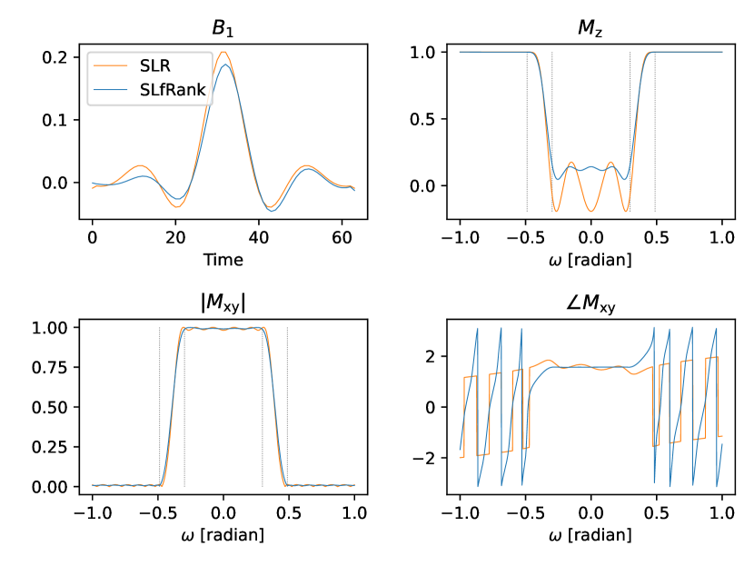
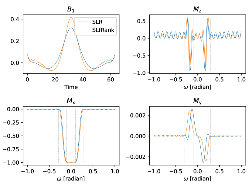
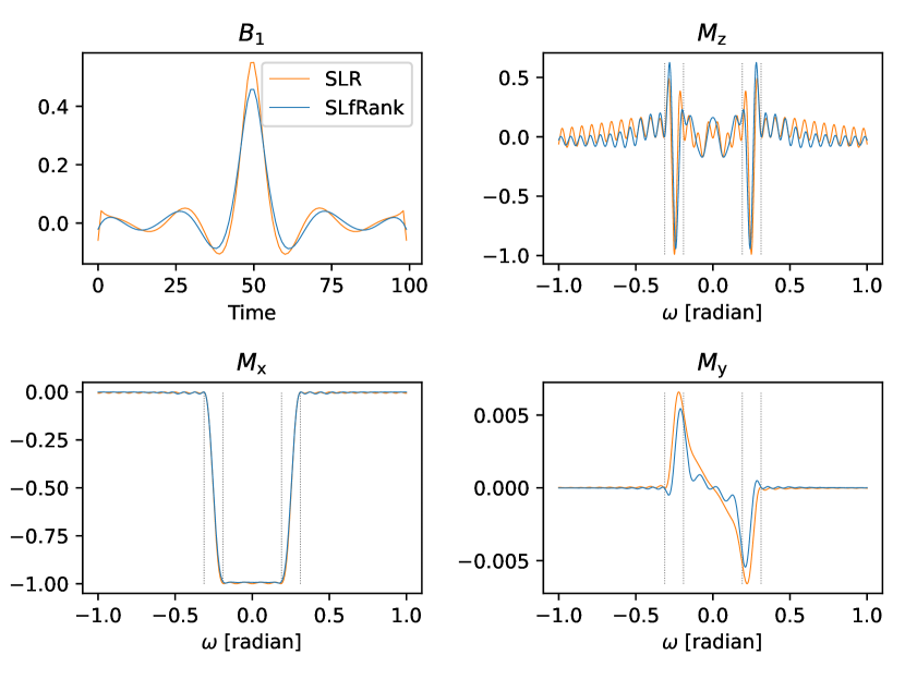
Figure 4 shows the linear phase excitation pulses and their magnetization profiles after refocusing. The SLfRank pulse has a much flatter phase response after refocusing than the SLR pulse. Pulse energy is reduced from 0.318 to 0.259 (18.6%) and peak is reduced from 0.208 to 0.189 (9.1%). Note that the SLfRank pulse is asymmetric, whereas the SLR pulse is symmetric. This shows that the proposed design compensates for the phase of α𝛼\alpha to generate a linear phase profile.

Refer to caption
Figure 4: Linear phase excitation pulses and their magnetization profiles after refocusing. The SLfRank pulse has a much flatter phase response than the original one after refocusing. Pulse energy is reduced from 0.318 to 0.259 (18.6%) and peak is reduced from 0.208 to 0.189 (9.1%). Note that the SLfRank pulse is asymmetric, whereas the SLR pulse is symmetric. This shows that the proposed design compensates for the phase of α𝛼\alpha to generate a linear phase profile.

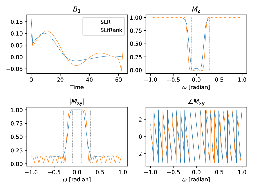
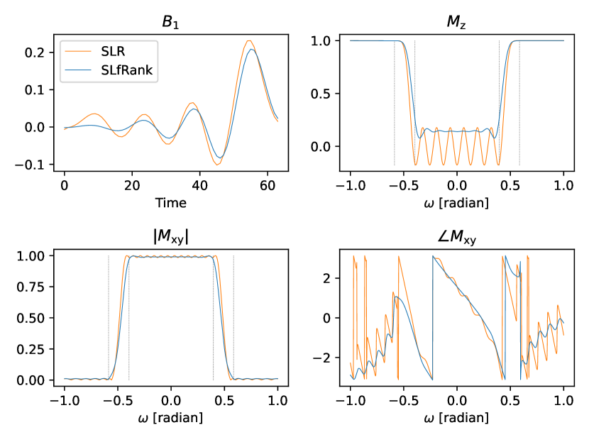
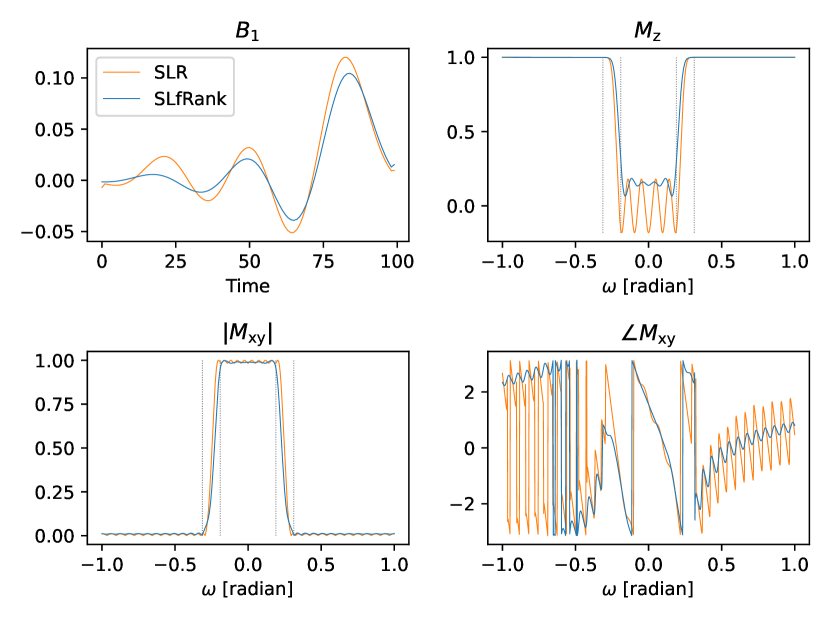
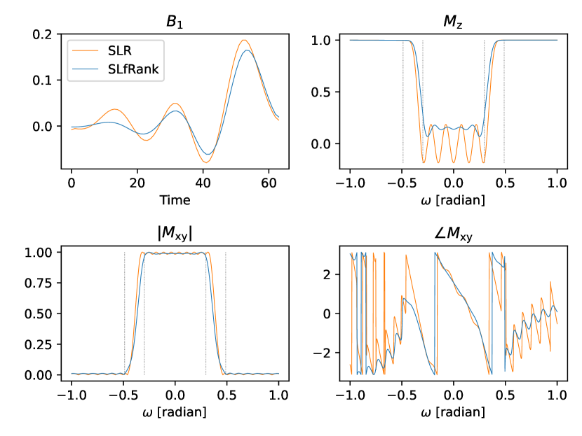
Figure 5 shows the minimum phase excitation pulses and their magnetization profiles. Pulse energy is reduced from 0.318 to 0.234 (26.4%) and peak is reduced from 0.187 to 0.165 (11.8%).
Refer to caption
Figure 5: Minimum phase slice selection pulses and their magnetization profiles. Pulse energy is reduced from 0.318 to 0.234 (26.4%) and peak is reduced from 0.187 to 0.165 (11.8%).

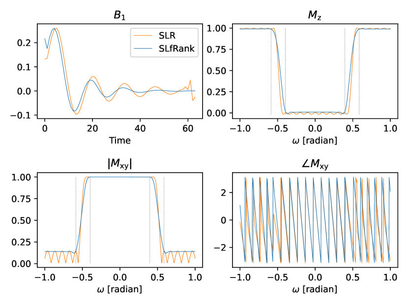
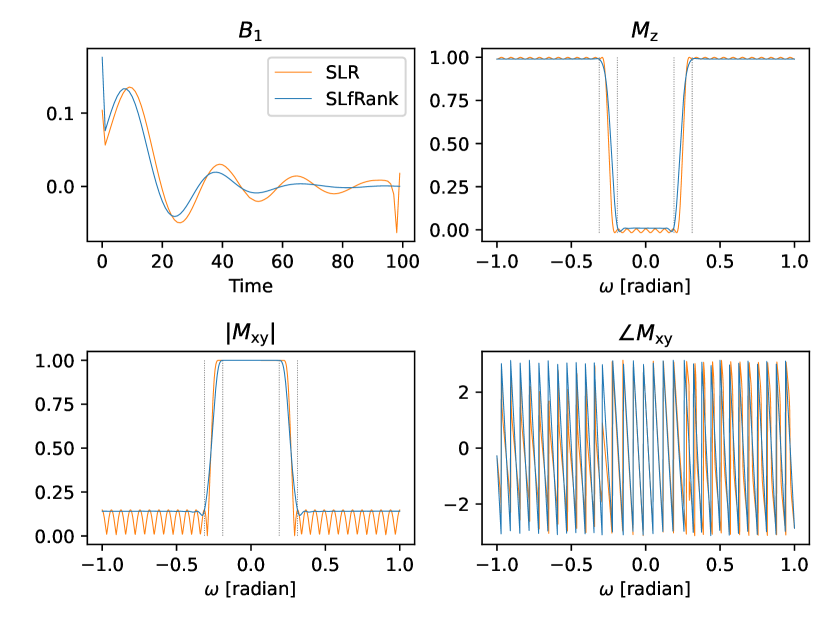
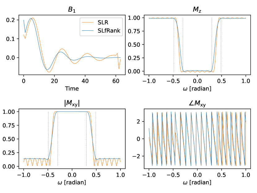
Figure 6 shows the maximum phase saturation pulses and their magnetization profiles. Pulse energy is reduced from 0.352 to 0.333 (5.40%) and peak is reduced from 0.212 to 0.208 (1.89%). The SLfRank pulse also has fewer discontinuities at the end of the pulse, commonly known as Connolly wings, when compared to the SLR pulse.
Refer to caption
Figure 6: Maximum phase saturation pulses and their magnetization profiles. Pulse energy is reduced from 0.352 to 0.333 (5.40%) and peak is reduced from 0.212 to 0.208 (1.89%). The SLfRank pulse also has fewer discontinuities at the end of the pulse, commonly known as Connolly wings, when compared to the SLR pulse.

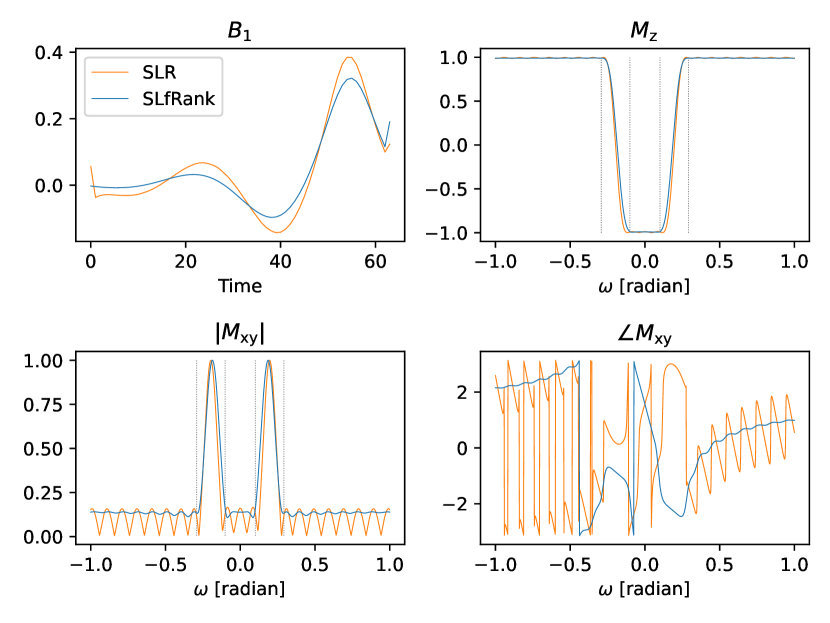
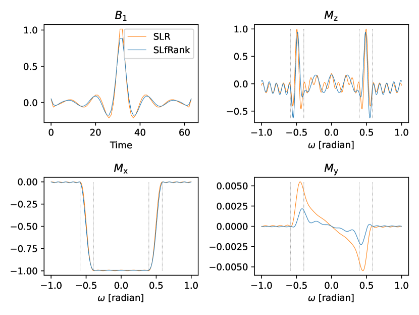
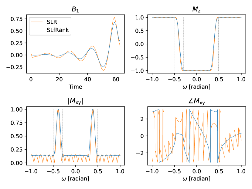
Figure 7 shows the minimum phase inversion pulses and their magnetization profiles. Pulse energy is reduced from 3.00 to 2.31 (23.0%) and peak is reduced from 0.781 to 0.679 (13.1%).
Refer to caption
Figure 7: Minimum phase inversion pulses and their magnetization profiles. Pulse energy is reduced from 3.00 to 2.31 (23.0%) and peak is reduced from 0.781 to 0.679 (13.1%).

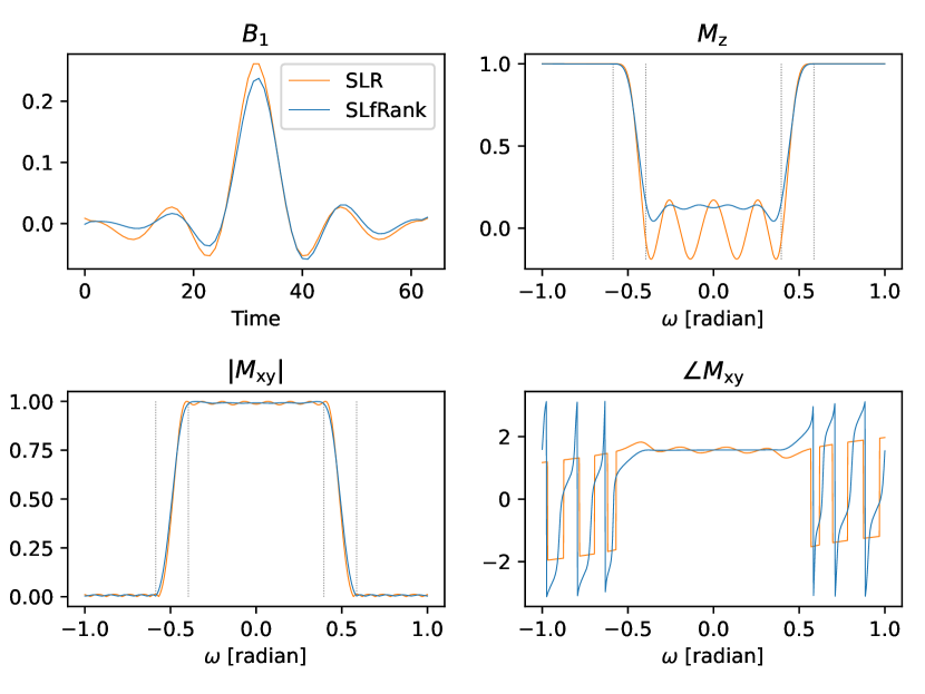
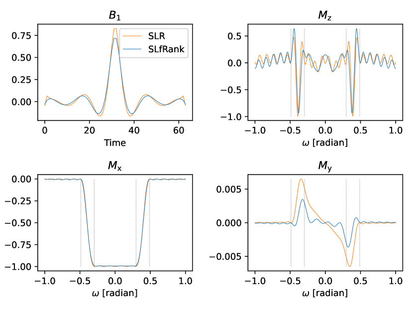
Finally, figure 8 shows the spin-echo refocusing pulses and their magnetization profiles. Pulse energy is reduced from 2.74 to 2.23 (18.6%) and peak is reduced from 0.827 to 0.716 (13.4%). The SLfRank pulse also has fewer discontinuities near the edges when compared to the SLR pulse.
Refer to caption
Figure 8: Spin-echo refocusing pulses and their magnetization profiles. Pulse energy is reduced from 2.74 to 2.23 (18.6%) and peak is reduced from 0.827 to 0.716 (13.4%). The SLfRank pulse also has fewer discontinuities near the edges when compared to the SLR pulse.

5 Phantom Experiment
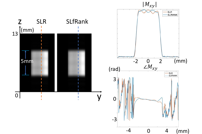
Refer to caption
Figure 9:
Refer to caption
Figure 10:
Refer to caption
Figure 11:

6 Discussion

Our results show that joint optimization of CK polynomials can produce pulses with reduced energy and more accurate phase profiles. In our opinion, reduced energy is the main feature of SLfRank pulses. Because SAR is proportional to pulse energy, SLfRank pulses can potentially accelerate acquisition time for SAR-limited sequences. In addition, there is a slight reduction of peak pulse amplitude, which can useful to prevent overflow in power amplifiers for simultaneous multi-slice imaging.

The accurate control over the transverse magnetization phase in SLfRank allows us to obtain a flatter phase response for slice excitation. However, this only provides marginal benefit in practice. As signals are contributed by summing across the excited slice, variation in the slice profile does not affect the resulting signal-to-noise ratio much. The SLfRank algorithm can still be useful for other applications, where pulse designers want to design more exotic phase profiles.

The proposed convex program can find a globally optimal solution for most examples in this manuscript. However, for the minimum phase excitation pulse design, there is still a slight gap between the solutions from the convex program and the rank-constrained problem. It is not clear to us whether this is a fundamental gap for such pulses. In particular, we observe that the convex program finds a rank-one solution when the ripple constraint is set to 2%percent22\%. It is possible that there is a regime where the convex program produces globally optimal pulses.

Compared to the original SLR algorithm, SLfRank takes much longer to compute. On a workstation with two 16-core Intel Xeon Silver 4216 processors, the original SLR algorithm takes less than a second to run, whereas the SLfRank algorithm takes around two minutes. Because most pulse designs are not done online on scanners, we believe the running time of SLfRank is reasonable. But there are also several directions to improve its computation time, including leveraging the fast Fourier transform in the iterative algorithm and using GPUs.

Finally, one limitation of both the SLR and SLfRank algorithms is that they assume the initial magnetization starts from equilibrium except for the special case of spin-echo refocusing with crusher gradients.

7 Conclusion

We have shown an improved SLR design process that can jointly solve for the CK polynomial pair. The new design can specify constraints directly on magnetization profiles, and optimize both CK polynomials to minimize pulse energy. The pulses in general have lower energy and fewer discontinuities. They also have more accurate phase responses when compared to the original SLR pulses. With lower energy pulses, the SLfRank algorithm can potentially accelerate SAR-limited sequences. Moreover, it allows users to design arbitrary excitation phase profiles, which opens up new research opportunities.

References

  • [1] K. Setsompop, J. Cohen-Adad, B. A. Gagoski, T. Raij, A. Yendiki, B. Keil, V. J. Wedeen, and L. L. Wald, “Improving diffusion mri using simultaneous multi-slice echo planar imaging,” Neuroimage, vol. 63, no. 1, pp. 569–580, 2012.
  • [2] H. Liu and G. B. Matson, “Radiofrequency pulse designs for three-dimensional mri providing uniform tipping in inhomogeneous b1 fields,” Magnetic resonance in medicine, vol. 66, no. 5, pp. 1254–1266, 2011.
  • [3] M. Shinnar and J. S. Leigh, “The application of spinors to pulse synthesis and analysis,” Magnetic Resonance in Medicine, vol. 12, no. 1, pp. 93–98, Oct. 1989. [Online]. Available: http://doi.wiley.com/10.1002/mrm.1910120112
  • [4] M. Shinnar, S. Eleff, H. Subramanian, and J. S. Leigh, “The synthesis of pulse sequences yielding arbitrary magnetization vectors,” Magnetic Resonance in Medicine, vol. 12, no. 1, pp. 74–80, Oct. 1989. [Online]. Available: http://doi.wiley.com/10.1002/mrm.1910120109
  • [5] M. Shinnar, L. Bolinger, and J. S. Leigh, “The synthesis of soft pulses with a specified frequency response,” Magnetic Resonance in Medicine, vol. 12, no. 1, pp. 88–92, Oct. 1989. [Online]. Available: http://doi.wiley.com/10.1002/mrm.1910120111
  • [6] ——, “Use of finite impulse response filters in pulse design,” in Proceedings of the 7th Annual Meeting and Exhibition of the Society for Magnetic Resonance in Medicine, San Francisco, CA, USA, 1988, p. 695, _eprint: https://onlinelibrary.wiley.com/doi/pdf/10.1002/mrmp.22419880204. [Online]. Available: https://onlinelibrary.wiley.com/doi/abs/10.1002/mrmp.22419880204
  • [7] ——, “The use of finite impulse response filters in pulse design,” Magnetic Resonance in Medicine, vol. 12, no. 1, pp. 81–87, Oct. 1989. [Online]. Available: http://doi.wiley.com/10.1002/mrm.1910120110
  • [8] P. Le Roux, “Exact Synthesis of Radiofrequency Waveforms,” in Proceedings of the 7th Annual Meeting and Exhibition of the Society for Magnetic Resonance in Medicine, San Francisco, CA, USA, Aug. 1988, p. 1049, _eprint: https://onlinelibrary.wiley.com/doi/pdf/10.1002/mrmp.22419880211. [Online]. Available: https://onlinelibrary.wiley.com/doi/abs/10.1002/mrmp.22419880211
  • [9] ——, “Method of radio-frequency excitation in an NMR experiment,” US Patent US4 940 940A, Jul., 1990, library Catalog: Google Patents. [Online]. Available: https://patents.google.com/patent/US4940940/en
  • [10] ——, “Simplified RF Synthesis,” in Proceedings of the 8th Annual Meeting and Exhibition of the Society for Magnetic Resonance in Medicine, vol. 1989, Amsterdam, The Netherlands, Aug. 1989, p. 1168, _eprint: https://onlinelibrary.wiley.com/doi/pdf/10.1002/mrmp.22419890305. [Online]. Available: https://onlinelibrary.wiley.com/doi/abs/10.1002/mrmp.22419890305
  • [11] J. Pauly, P. L. Roux, D. Nishimura, and A. Macovski, “Parameter relations for the Shinnar-Le Roux selective excitation pulse design algorithm (NMR imaging),” IEEE Transactions on Medical Imaging, vol. 10, no. 1, pp. 53–65, Mar. 1991.
  • [12] J. K. Barral, J. M. Pauly, and D. G. Nishimura, “SLR RF Pulse Design for Arbitrarily-Shaped Excitation Profiles,” in Proceedings of the ISMRM 16th Annual Meeting, Toronto, ON, Canada, May 2008, p. 1323.
  • [13] C. L. Epstein, “Introduction to magnetic resonance imaging for mathematicians,” Annales de l’institut Fourier, vol. 54, no. 5, pp. 1697–1716, 2004. [Online]. Available: https://aif.centre-mersenne.org/item/AIF_2004__54_5_1697_0/
  • [14] C. L. Epstein and J. F. Magland, “Inverse Scattering Pulse Design,” in eMagRes.   American Cancer Society, 2012, _eprint: https://onlinelibrary.wiley.com/doi/pdf/10.1002/9780470034590.emrstm1303. [Online]. Available: http://onlinelibrary.wiley.com/doi/abs/10.1002/9780470034590.emrstm1303
  • [15] C. L. Epstein, “Minimum energy pulse synthesis via the inverse scattering transform,” Journal of Magnetic Resonance, vol. 167, no. 2, pp. 185–210, Apr. 2004. [Online]. Available: https://linkinghub.elsevier.com/retrieve/pii/S1090780703004439
  • [16] ——, “Minimum energy pulse synthesis via the inverse scattering transform,” Journal of Magnetic Resonance, vol. 167, no. 2, pp. 185–210, Apr. 2004. [Online]. Available: http://linkinghub.elsevier.com/retrieve/pii/S1090780703004439
  • [17] J. F. Magland, “Discrete Inverse Scattering Theory for NMR Pulse Design,” arXiv:0903.4363 [math-ph], Mar. 2009, arXiv: 0903.4363. [Online]. Available: http://arxiv.org/abs/0903.4363
  • [18] J. Magland and C. L. Epstein, “Exact half pulse synthesis via the inverse scattering transform,” Journal of Magnetic Resonance, vol. 171, no. 2, pp. 305–313, Dec. 2004. [Online]. Available: https://linkinghub.elsevier.com/retrieve/pii/S1090780704003040
  • [19] ——, “Practical pulse synthesis via the discrete inverse scattering transform,” Journal of Magnetic Resonance, vol. 172, no. 1, pp. 63–78, Jan. 2005. [Online]. Available: http://linkinghub.elsevier.com/retrieve/pii/S1090780704002800
  • [20] S. Conolly, D. Nishimura, and A. Macovski, “Optimal Control Solutions to the Magnetic Resonance Selective Excitation Problem,” IEEE Transactions on Medical Imaging, vol. 5, no. 2, pp. 106–115, Jun. 1986.
  • [21] M. X. Goemans and D. P. Williamson, “Improved approximation algorithms for maximum cut and satisfiability problems using semidefinite programming,” Journal of the ACM, vol. 42, no. 6, pp. 1115–1145, Nov. 1995. [Online]. Available: https://dl.acm.org/doi/10.1145/227683.227684
  • [22] E. J. Candes and T. Tao, “The Power of Convex Relaxation: Near-Optimal Matrix Completion,” IEEE Transactions on Information Theory, vol. 56, no. 5, pp. 2053–2080, May 2010. [Online]. Available: http://ieeexplore.ieee.org/document/5452187/
  • [23] E. J. Candès, Y. C. Eldar, T. Strohmer, and V. Voroninski, “Phase Retrieval via Matrix Completion,” SIAM Journal on Imaging Sciences, vol. 6, no. 1, pp. 199–225, Jan. 2013. [Online]. Available: http://epubs.siam.org/doi/10.1137/110848074
  • [24] B. Dumitrescu, Positive trigonometric polynomials and signal processing applications, ser. Signals and communication technology.   Dordrecht: Springer, 2007, oCLC: 85842464.
  • [25] S. Diamond and S. Boyd, “CVXPY: a python-embedded modeling language for convex optimization,” The Journal of Machine Learning Research, vol. 17, no. 1, pp. 2909–2913, Jan. 2016.
  • [26] A. Chambolle and T. Pock, “A First-Order Primal-Dual Algorithm for Convex Problems with Applications to Imaging,” Journal of Mathematical Imaging and Vision, vol. 40, no. 1, pp. 120–145, May 2011. [Online]. Available: http://link.springer.com/10.1007/s10851-010-0251-1
  • [27] F. Ong and M. Lustig, “SigPy: A Python Package for High Performance Iterative Reconstruction,” in Proceedings of the ISMRM 27th Annual Meeting, Montreal, Quebec, Canada, May 2019, p. 4819. [Online]. Available: https://cds.ismrm.org/protected/19MPresentations/abstracts/4819.html
  • [28] J. B. Martin, F. Ong, J. Ma, J. I. Tamir, M. Lustig, and W. A. Grissom, “SigPy.RF: Comprehensive Open-Source RF Pulse Design Tools for Reproducible Research,” in Proceedings of the ISMRM 16th Annual Meeting, Virtual, Aug. 2020, p. 1045.

Supplementary Material

RF Pulses with TBW=4 and n=64
Refer to caption
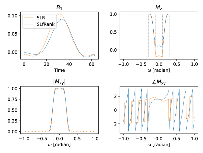
Figure 12: Linear phase excitation pulses and their magnetization profiles after gradient refocusing with TBW=4. Pulse energy is reduced from 0.157 to 0.114 (27.4%) and peak is reduced from 0.104 to 0.090 (13.5%).
Refer to caption
Figure 13: Minimum phase excitation pulses with TBW=4. Pulse energy is reduced from 0.143 to 0.089 (37.8%) and peak is reduced from 0.094 to 0.075 (20.2%).
Refer to caption
Figure 14: Maximum phase saturation pulses with TBW=4. Pulse energy is reduced from 0.179 to 0.157 (12.3%). Peak is increased from 0.110 to 0.168 (52.7%).
Refer to caption
Figure 15: Minimum phase inversion pulses with TBW=4. Pulse energy is reduced from 1.338 to 0.992 (25.9%) and peak is reduced from 0.385 to 0.322 (16.4%).
Refer to caption
Figure 16: Zero phase spin-echo refocusing pulses with TBW=4. Pulse energy is reduced from 1.289 to 0.932 (27.7%) and peak is reduced from 0.416 to 0.320 (23.1%).

RF Pulses with TBW=10 and n=64
Refer to caption
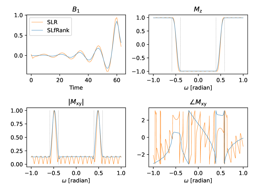
Figure 17: Linear phase excitation pulses and their magnetization profiles after gradient refocusing with TBW=10. Pulse energy is reduced from 0.259 to 0.212 (18.1%) and peak is reduced from 0.169 to 0.153 (9.47%).
Refer to caption
Figure 18: Minimum phase excitation pulses with TBW=10. Pulse energy is reduced from 0.259 to 0.194 (25.1%) and peak is reduced from 0.149 to 0.132 (17.0%).
Refer to caption
Figure 19: Maximum phase saturation pulses with TBW=10. Pulse energy is reduced from 0.295 to 0.275 (6.78%). Peak is increased from 0.167 to 0.186 (12.7%).
Refer to caption
Figure 20: Minimum phase inversion pulses with TBW=10. Pulse energy is reduced from 2.440 to 1.910 (21.7%) and peak is reduced from 0.624 to 0.549 (12.0%).
Refer to caption
Figure 21: Zero phase spin-echo refocusing pulses with TBW=10. Pulse energy is reduced from 2.263 to 1.794 (20.7%) and peak is reduced from 0.687 to 0.579 (15.7%).

RF Pulses with TBW=8 and n=100
Refer to caption
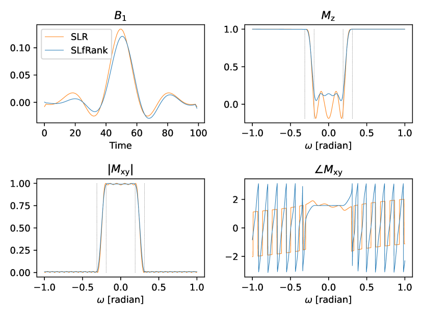
Figure 22: Linear phase excitation pulses and their magnetization profiles after gradient refocusing with n=100𝑛100n=100. Pulse energy is reduced from 0.204 to 0.166 (18.6%) and peak is reduced from 0.134 to 0.121 (9.70%).
Refer to caption
Figure 23: Minimum phase excitation pulses with n=100𝑛100n=100. Pulse energy is reduced from 0.203 to 0.148 (27.1%) and peak is reduced from 0.120 to 0.105 (12.5%).
Refer to caption
Figure 24: Maximum phase saturation pulses with n=100𝑛100n=100. Pulse energy is reduced from 0.229 to 0.220 (3.94%). Peak is increased from 0.135 to 0.176 (30.4%).
Refer to caption
Figure 25: Minimum phase inversion pulses with n=100𝑛100n=100. Pulse energy is reduced from 1.938 to 1.489 (23.2%) and peak is reduced from 0.507 to 0.435 (14.2%).
Refer to caption
Figure 26: Zero phase spin-echo refocusing pulses with n=100𝑛100n=100. Pulse energy is reduced from 1.778 to 1.390 (21.8%) and peak is reduced from 0.550 to 0.458 (16.7%).

Proof Sketch for Equation (14)

Here we provide a proof sketch to show that for any matrix 𝐌n×n𝐌superscript𝑛𝑛\mathbf{M}\in\mathbb{C}^{n\times n}, the following two equations are equivalent:

1=𝝍(eıω)𝐌𝝍(eıω) for all ω1superscript𝝍superscript𝑒italic-ı𝜔𝐌𝝍superscript𝑒italic-ı𝜔 for all 𝜔1=\bm{\psi}^{*}(e^{\imath\omega})\mathbf{M}\bm{\psi}(e^{\imath\omega})\text{ for all }\omega

where 𝝍(z)=(1eıωeıωn)T𝝍𝑧superscriptmatrix1superscript𝑒italic-ı𝜔superscript𝑒italic-ı𝜔𝑛𝑇\bm{\psi}(z)=\begin{pmatrix}1&e^{\imath\omega}&\ldots&e^{\imath\omega n}\end{pmatrix}^{T}, and

i,j:ij=k(𝐌)ij={1,if k=00,otherwise,subscript:𝑖𝑗𝑖𝑗𝑘subscript𝐌𝑖𝑗cases1if 𝑘00otherwise\sum_{i,j:i-j=k}(\mathbf{M})_{ij}=\begin{cases}1,&\text{if }k=0\\ 0,&\text{otherwise}\end{cases},

for k=n,n+1,,n𝑘𝑛𝑛1𝑛k=-n,-n+1,\ldots,n.

Let us define 𝟏1\mathbf{1} to be an all-one vector and direct-product\odot be the element-wise product, then

𝝍(z)𝐌𝝍(eıω)=𝟏(𝐌[𝝍(eıω)𝝍(eıω)])𝟏.superscript𝝍𝑧𝐌𝝍superscript𝑒italic-ı𝜔superscript1direct-product𝐌delimited-[]𝝍superscript𝑒italic-ı𝜔superscript𝝍superscript𝑒italic-ı𝜔1\bm{\psi}^{*}(z)\mathbf{M}\bm{\psi}(e^{\imath\omega})=\mathbf{1}^{*}\left(\mathbf{M}\odot\left[\bm{\psi}(e^{\imath\omega})\bm{\psi}^{*}(e^{\imath\omega})\right]\right)\mathbf{1}.

A special structure of the matrix 𝝍(eıω)𝝍(eıω)𝝍superscript𝑒italic-ı𝜔superscript𝝍superscript𝑒italic-ı𝜔\bm{\psi}(e^{\imath\omega})\bm{\psi}^{*}(e^{\imath\omega}) is that each of its sub-diagonal has the same value of a phase exponential. That is,

(𝝍(eıω)𝝍(eıω))ij=eıω(ij)subscript𝝍superscript𝑒italic-ı𝜔superscript𝝍superscript𝑒italic-ı𝜔𝑖𝑗superscript𝑒italic-ı𝜔𝑖𝑗\left(\bm{\psi}(e^{\imath\omega})\bm{\psi}^{*}(e^{\imath\omega})\right)_{ij}=e^{\imath\omega(i-j)}

for i,j=1,,nformulae-sequence𝑖𝑗1𝑛i,j=1,\ldots,n.

Hence 𝟏𝐌[𝝍(eıω)𝝍(eıω)]𝟏direct-productsuperscript1𝐌delimited-[]𝝍superscript𝑒italic-ı𝜔superscript𝝍superscript𝑒italic-ı𝜔1\mathbf{1}^{*}\mathbf{M}\odot\left[\bm{\psi}(e^{\imath\omega})\bm{\psi}^{*}(e^{\imath\omega})\right]\mathbf{1} is the same as the inner product between a vector 𝐯𝐯\mathbf{v} formed by diagonally summing 𝐌𝐌\mathbf{M} and a linear phase vector ϕ(eıω)=[eıωn,,eıω(n1),eıωn]Tbold-italic-ϕsuperscript𝑒italic-ı𝜔superscriptsuperscript𝑒italic-ı𝜔𝑛superscript𝑒italic-ı𝜔𝑛1superscript𝑒italic-ı𝜔𝑛𝑇\bm{\phi}(e^{\imath\omega})=[e^{-\imath\omega n},\ldots,e^{\imath\omega(n-1)},e^{\imath\omega n}]^{T}. In particular, 𝐯𝐯\mathbf{v} is defined as

(𝐯)k+n+1=i,j:ij=k(𝐌)ijsubscript𝐯𝑘𝑛1subscript:𝑖𝑗𝑖𝑗𝑘subscript𝐌𝑖𝑗(\mathbf{v})_{k+n+1}=\sum_{i,j:i-j=k}(\mathbf{M})_{ij}

for k=n,n+1,,n𝑘𝑛𝑛1𝑛k=-n,-n+1,\ldots,n.

Finally, to satisfy 1=𝝍(eıω)𝐌𝝍(eıω)1superscript𝝍superscript𝑒italic-ı𝜔𝐌𝝍superscript𝑒italic-ı𝜔1=\bm{\psi}^{*}(e^{\imath\omega})\mathbf{M}\bm{\psi}(e^{\imath\omega}) for all ω𝜔\omega, one must have (𝐯)n+1subscript𝐯𝑛1(\mathbf{v})_{n+1} being one and all other values being zero. This is equivalent to have main diagonal sum of 𝐌𝐌\mathbf{M} being one, but all other sub-diagonal sum being zero.

Convergence Plot

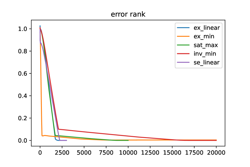
To show the convergence process of the algorithm, the error rank of different RF pulse design types was plotted, which was defined as:

errorrank=𝐏(𝐚𝐛)(𝐚𝐛)2𝑒𝑟𝑟𝑜𝑟𝑟𝑎𝑛𝑘subscriptnorm𝐏matrix𝐚𝐛matrixsuperscript𝐚superscript𝐛2error\ rank=\left\|\mathbf{P}-\begin{pmatrix}\mathbf{a}\\ \mathbf{b}\end{pmatrix}\begin{array}[]{@{}c@{}}\begin{pmatrix}\mathbf{a}^{*}&\mathbf{b}^{*}\end{pmatrix}\\ \mathstrut\end{array}\right\|_{2}

The plot shows that the convex program always converges, however, minimum phase designs take more iterations.
Refer to caption
Figure 27: Convergence plot of the different RF pulse designs using the proposed algorithm. In most cases, the algorithm will converge around 2000 iterations.