Helmholtzian Eigenmap: Topological feature discovery & edge flow learning from point cloud data

Yu-Chia Chen
Meta Platforms, Inc.
Seattle, WA 98109
yuchaz@uw.edu
&Weicheng Wu
Department of Statistics
University of Washington
Seattle, WA 98195
weich555@uw.edu
&Marina Meilă
Department of Statistics
University of Washington
Seattle, WA 98195
mmp2@uw.edu
&Ioannis G. Kevrekidis
Chemical and Biomolecular Engineering &
Applied Mathematics and Statistics
Johns Hopkins University
Baltimore, MD 21218
yannisk@jhu.edu
Abstract

The manifold Helmholtzian (1-Laplacian) operator Δ1subscriptΔ1\Delta_{1} elegantly generalizes the Laplace-Beltrami operator to vector fields on a manifold {\mathcal{M}}. In this work, we propose the estimation of the manifold Helmholtzian from point cloud data by a weighted 1-Laplacian 1subscript1\mathbf{\mathcal{L}}_{1}. While higher order Laplacians have been introduced and studied, this work is the first to present a graph Helmholtzian constructed from a simplicial complex as a consistent estimator for the continuous operator in a non-parametric setting. Equipped with the geometric and topological information about {\mathcal{M}}, the Helmholtzian is a useful tool for the analysis of flows and vector fields on {\mathcal{M}} via the Helmholtz-Hodge theorem. In addition, the 1subscript1\mathbf{\mathcal{L}}_{1} allows the smoothing, prediction, and feature extraction of the flows. We demonstrate these possibilities on substantial sets of synthetic and real point cloud datasets with non-trivial topological structures; and provide theoretical results on the limit of 1subscript1\mathbf{\mathcal{L}}_{1} to Δ1subscriptΔ1\Delta_{1}.

1 Motivation

In this paper we initiate the estimation of higher order Laplacian operators from point cloud data, with a focus on the first order Laplacian operator Δ1subscriptΔ1\Delta_{1} of a manifold. Laplacians are known to be intimately tied to a manifold’s topology and geometry. While the Laplace-Beltrami operator Δ0subscriptΔ0\Delta_{0}, an operator acting on functions (00-forms), is well studied and pivotal in classical manifold learning; estimating the 111-Laplacian Δ1subscriptΔ1\Delta_{1}, an operator acting on vector fields (111-forms), for a manifold has rarely been attempted yet. Order k𝑘k Laplacian operators (on k𝑘k-forms), denoted ΔksubscriptΔ𝑘\Delta_{k}, exist as well, for k=1,2,𝑘12k=1,2,\ldots.

The discrete operator analogue of ΔksubscriptΔ𝑘\Delta_{k}, known as the k𝑘k-Hodge Laplacian matrix 𝐋ksubscript𝐋𝑘\mathbf{L}_{k}, has been proposed more than 7 decades ago [Eck44]. The beauty of the aforementioned framework generated numerous applications in areas such as numerical analysis [AFW10, Dod76], edge flow learning on graphs [SBH+20, JSSB19], pairwise ranking [JLYY11], and game theory [CMOP11].

Being able to estimate Δ1subscriptΔ1\Delta_{1} by a discrete Helmholtzian 1subscript1\mathbf{\mathcal{L}}_{1} acting on the edges of a graph can support many applications, just as the Δ0subscriptΔ0\Delta_{0} estimator by weighted Laplacians successfully did. For instance, (\romannum1) topological information, i.e., the first Betti number β1subscript𝛽1\beta_{1} [Lim20], can be obtained by the dimension of the null space of 1subscript1\mathbf{\mathcal{L}}_{1}; (\romannum2) low dimensional representation of the space of vector fields on a manifold are made possible, similar to the dimensionality reduction algorithms such as Laplacian Eigenmap from the discrete estimates of Δ0subscriptΔ0\Delta_{0}; (\romannum3) the well known Helmholtz-Hodge decompositon (HHD) [BNPB13, Lim20] allows us to test, e.g., if a vector field on the manifold {\mathcal{M}} is approximately a gradient or a rotational field; lastly (\romannum4), edge flow semi-supervised learning (SSL) and unsupervised learning algorithms, i.e., flow prediction and flow smoothing in edge space, can be easily derived from the well-studied node based learning models [BNS06, OFK+18] with the aid of 1subscript1\mathbf{\mathcal{L}}_{1}.

In this work, we propose a discrete estimator (1subscript1\mathbf{\mathcal{L}}_{1}) of the Helmholtzian Δ1subscriptΔ1\Delta_{1} with proper triangular weights which resembles the well known Vietoris-Rips (VR) complex in the persistent homology theory. We show separately the (pointwise) convergence of the down and the up components of the discrete graph Helmholtzian 1subscript1\mathbf{\mathcal{L}}_{1} to the continuous operators Δ1downsuperscriptsubscriptΔ1down\Delta_{1}^{\rm down} and Δ1upsuperscriptsubscriptΔ1up\Delta_{1}^{\rm up}. In addition, we present several applications to graph signal processing and semi-supervised learning algorithms on the edge flows with the constructed 1subscript1\mathbf{\mathcal{L}}_{1}. We support our theoretical claims and illustrate the versatility of the proposed Δ1subscriptΔ1\Delta_{1} estimator with extensive empirical results on synthetic and real datasets with non-trivial manifold structures.

In the next section we briefly introduce Hodge theory and higher order Laplacians. Section 3 presents the 1subscript1\mathbf{\mathcal{L}}_{1} construction algorithm. The theoretical results are in Section 4. Sections 6 and 7 provide several applications of the estimated Helmholtzian to the analysis of vector fields. Those Figure/Table/Equation/Theorem references with prefix S are in the Supplement.

2 Background: Hodge theory

Simplicial complex

A natural extension of a graph to higher dimensional relations is called a simplicial complex. Define a k𝑘k-simplex to be a k𝑘k-dimensional polytope which is the convex hull of its k+1𝑘1k+1 (affinely independent) vertices. A simplicial complex SCSC\mathrm{SC} is a set of simplices such that every face of a simplex from SCSC\mathrm{SC} is also in SCSC\mathrm{SC}. Let ΣksubscriptΣ𝑘\Sigma_{k} be the collection of k𝑘k-simplices σksubscript𝜎𝑘\sigma_{k} of SCSC\mathrm{SC}; we write SC=(Σ0,Σ1,,Σ)SCsubscriptΣ0subscriptΣ1subscriptΣ\mathrm{SC}=(\Sigma_{0},\Sigma_{1},\cdots,\Sigma_{\ell}), with nk=|Σk|subscript𝑛𝑘subscriptΣ𝑘n_{k}=|\Sigma_{k}|. A graph is G=(V,E)=(Σ0,Σ1)𝐺𝑉𝐸subscriptΣ0subscriptΣ1G=(V,E)=(\Sigma_{0},\Sigma_{1}), with n0=|V|=nsubscript𝑛0𝑉𝑛n_{0}=|V|=n. In this work, we focus on dimension k2𝑘2k\leq 2 and simplicial complexes of the form SC2=(V,E,T)(Σ0,Σ1,Σ2)subscriptSC2𝑉𝐸𝑇subscriptΣ0subscriptΣ1subscriptΣ2\mathrm{SC}_{2}=(V,E,T)\equiv(\Sigma_{0},\Sigma_{1},\Sigma_{2}), where T𝑇T is the set of triangles of SCSC\mathrm{SC}.

k𝑘k (co-)chain

Given an arbitrary orientation for each simplex σikΣksuperscriptsubscript𝜎𝑖𝑘subscriptΣ𝑘\sigma_{i}^{k}\in\Sigma_{k}, one can define the finite-dimensional vector space 𝒞ksubscript𝒞𝑘\mathcal{C}_{k} over ΣksubscriptΣ𝑘\Sigma_{k} with coefficients in \mathbb{R}. An element ωk𝒞ksubscript𝜔𝑘subscript𝒞𝑘\mathbf{\omega}_{k}\in\mathcal{C}_{k} is called a k𝑘k-chain and can be written as ωk=iωk,iσiksubscript𝜔𝑘subscript𝑖subscript𝜔𝑘𝑖subscriptsuperscript𝜎𝑘𝑖\mathbf{\omega}_{k}=\sum_{i}\omega_{k,i}\sigma^{k}_{i}. Since 𝒞ksubscript𝒞𝑘\mathcal{C}_{k} is isomorphic to nksuperscriptsubscript𝑛𝑘\mathbb{R}^{n_{k}}, ωksubscript𝜔𝑘\mathbf{\omega}_{k} can be represented by a vector of coordinates ωk=(ωk,1,,ωk,nk)nksubscript𝜔𝑘superscriptsubscript𝜔𝑘1subscript𝜔𝑘subscript𝑛𝑘topsuperscriptsubscript𝑛𝑘\mathbf{\omega}_{k}=(\omega_{k,1},\cdots,\omega_{k,n_{k}})^{\top}\in\mathbb{R}^{n_{k}}. 𝒞ksuperscript𝒞𝑘\mathcal{C}^{k} denotes the dual space of 𝒞ksubscript𝒞𝑘\mathcal{C}_{k}; an element of ωk𝒞ksuperscript𝜔𝑘superscript𝒞𝑘\mathbf{\omega}^{k}\in\mathcal{C}^{k} is called a k𝑘k-cochain. Even though they are intrinsically different, we will use chains and cochains interchangeably for simplicity in this work. Readers are encouraged to consult [Lim20] for thorough discussions on the distinction between these two terms.

(Co-)boundary map

The boundary map (operator) k:𝒞k𝒞k1:subscript𝑘subscript𝒞𝑘subscript𝒞𝑘1\mathcal{B}_{k}:\mathcal{C}_{k}\to\mathcal{C}_{k-1} (defined rigorously in the Supplement C) maps a simplex σksubscript𝜎𝑘\sigma_{k} to the k1𝑘1k-1-chain of its faces, with signs given by the orientation of the simplex w.r.t. each face. For example, let x,y,zV𝑥𝑦𝑧𝑉x,y,z\in V, edges [x,y],[y,z],[x,z]E𝑥𝑦𝑦𝑧𝑥𝑧𝐸[x,y],[y,z],[x,z]\in E, and a triangle t=[x,y,z]T𝑡𝑥𝑦𝑧𝑇t=[x,y,z]\in T, we have B2(t)=[x,y]+[y,z][x,z]subscript𝐵2𝑡𝑥𝑦𝑦𝑧𝑥𝑧B_{2}(t)=[x,y]+[y,z]-[x,z]. Since 𝒞ksubscript𝒞𝑘\mathcal{C}_{k} is isomorphic to nksuperscriptsubscript𝑛𝑘\mathbb{R}^{n_{k}}, one can represent ksubscript𝑘\mathcal{B}_{k} by a boundary map (matrix) 𝐁k{0,±1}nk1×nksubscript𝐁𝑘superscript0plus-or-minus1subscript𝑛𝑘1subscript𝑛𝑘\mathbf{B}_{k}\in\{0,\pm 1\}^{n_{k-1}\times n_{k}}. The entry (𝐁k)σk1,σksubscriptsubscript𝐁𝑘subscript𝜎𝑘1subscript𝜎𝑘(\mathbf{B}_{k})_{\sigma_{k-1},\sigma_{k}} represents the orientation of σk1subscript𝜎𝑘1\sigma_{k-1} as a face of σksubscript𝜎𝑘\sigma_{k}, or equals 0 when the two are not adjacent. For k=1𝑘1k=1, the boundary map is the node to edge graph incidence matrix, i.e., (𝐁1)[a],[xy]=1subscriptsubscript𝐁1delimited-[]𝑎delimited-[]𝑥𝑦1({\mathbf{B}}_{1})_{[a],[xy]}=1 if a=x𝑎𝑥a=x, (𝐁1)[a],[x,y]=1subscriptsubscript𝐁1delimited-[]𝑎𝑥𝑦1({\mathbf{B}}_{1})_{[a],[x,y]}=-1 if a=y𝑎𝑦a=y, and zero otherwise; for k=2𝑘2k=2, each column of 𝐁2subscript𝐁2\mathbf{B}_{2} contains the orientation of a triangle w.r.t. its edges. In other words, (𝐁2)[a,b],[x,y,z]=1subscriptsubscript𝐁2𝑎𝑏𝑥𝑦𝑧1({\mathbf{B}}_{2})_{[a,b],[x,y,z]}=1 if [a,b]{[x,y],[y,z]}𝑎𝑏𝑥𝑦𝑦𝑧[a,b]\in\{[x,y],[y,z]\}, (𝐁2)[a,b],[x,y,z]=1subscriptsubscript𝐁2𝑎𝑏𝑥𝑦𝑧1({\mathbf{B}}_{2})_{[a,b],[x,y,z]}=-1 if [a,b]=[x,z]𝑎𝑏𝑥𝑧[a,b]=[x,z], and 00 otherwise. In this paper, we will only work with simplices up to dimension k=2𝑘2k=2. Closely related to boundary map is the co-boundary map. This operator is the adjoint of the boundary map and it maps a simplex to its co-faces, i.e., k:𝒞k1𝒞k:superscript𝑘superscript𝒞𝑘1superscript𝒞𝑘\mathcal{B}^{k}:\mathcal{C}^{k-1}\to\mathcal{C}^{k}. The corresponding co-boundary matrix is simply the transpose of the boundary matrix, i.e., 𝐁ksuperscriptsubscript𝐁𝑘top\mathbf{B}_{k}^{\top}. Pseudocode for constructing 𝐁ksubscript𝐁𝑘\mathbf{B}_{k} can be found in Algorithm 2.

The discrete k𝑘k-Laplacian

The unnormalized k𝑘k-Laplacian 𝐋k=𝐁k𝐁k+𝐁k+1𝐁k+1subscript𝐋𝑘superscriptsubscript𝐁𝑘topsubscript𝐁𝑘subscript𝐁𝑘1superscriptsubscript𝐁𝑘1top\mathbf{L}_{k}=\mathbf{B}_{k}^{\top}\mathbf{B}_{k}+\mathbf{B}_{k+1}\mathbf{B}_{k+1}^{\top} was first introduced by [Eck44] as a discrete analog to ΔksubscriptΔ𝑘\Delta_{k}. One can verify that 𝐋0=𝐁1𝐁1subscript𝐋0subscript𝐁1superscriptsubscript𝐁1top\mathbf{L}_{0}=\mathbf{B}_{1}\mathbf{B}_{1}^{\top} represents the unnormalized graph Laplacian [Chu96]. To extend the aforementioned construction to a weighted k𝑘k-Laplacian, one can introduce a diagonal non-negative weight matrix 𝐖ksubscript𝐖𝑘{\mathbf{W}}_{k} of dimension nksubscript𝑛𝑘n_{k}, with (𝐖k)[σk,σk]subscriptsubscript𝐖𝑘subscript𝜎𝑘subscript𝜎𝑘(\mathbf{W}_{k})_{[\sigma_{k},\sigma_{k}]} being the weight for simplex σksubscript𝜎𝑘\sigma_{k}. For unweighted k𝑘k-Laplacians, 𝐖k1,𝐖k,𝐖k+1subscript𝐖𝑘1subscript𝐖𝑘subscript𝐖𝑘1\mathbf{W}_{k-1},\mathbf{W}_{k},\mathbf{W}_{k+1} are equal to the unit matrices. By analogy to the random walk graph Laplacian, [HJ13] define a (weighted) random walk k𝑘k-Hodge Laplacian by k=𝐁k𝐖k11𝐁k𝐖k+𝐖k1𝐁k+1𝐖k+1𝐁k+1.subscript𝑘superscriptsubscript𝐁𝑘topsuperscriptsubscript𝐖𝑘11subscript𝐁𝑘subscript𝐖𝑘superscriptsubscript𝐖𝑘1subscript𝐁𝑘1subscript𝐖𝑘1superscriptsubscript𝐁𝑘1top\mathbf{\mathcal{L}}_{k}=\mathbf{B}_{k}^{\top}\mathbf{W}_{k-1}^{-1}\mathbf{B}_{k}\mathbf{W}_{k}+\mathbf{W}_{k}^{-1}\mathbf{B}_{k+1}\mathbf{W}_{k+1}\mathbf{B}_{k+1}^{\top}. Of specific interest to us are the weighted Laplacians for k=0𝑘0k=0 (graph Laplacian) and k=1𝑘1k=1 (graph Helmholtzian). The operator 0=𝐖01𝐁1𝐖1𝐁1subscript0superscriptsubscript𝐖01subscript𝐁1subscript𝐖1superscriptsubscript𝐁1top\mathbf{\mathcal{L}}_{0}=\mathbf{W}_{0}^{-1}\mathbf{B}_{1}\mathbf{W}_{1}\mathbf{B}_{1}^{\top} coincides with the random walk graph Laplacian [Chu96]. The Helmholtzian is defined as

1=a𝐁1𝐖01𝐁1𝐖11down+b𝐖11𝐁2𝐖2𝐁21up.subscript1𝑎subscriptsuperscriptsubscript𝐁1topsuperscriptsubscript𝐖01subscript𝐁1subscript𝐖1superscriptsubscript1down𝑏subscriptsuperscriptsubscript𝐖11subscript𝐁2subscript𝐖2superscriptsubscript𝐁2topsuperscriptsubscript1up\mathbf{\mathcal{L}}_{1}=a\cdot\underbrace{{\mathbf{B}}_{1}^{\top}{\mathbf{W}}_{0}^{-1}{\mathbf{B}}_{1}{\mathbf{W}}_{1}}_{\mathbf{\mathcal{L}}_{1}^{\mathrm{down}}}+b\cdot\underbrace{{\mathbf{W}}_{1}^{-1}{\mathbf{B}}_{2}{\mathbf{W}}_{2}{\mathbf{B}}_{2}^{\top}}_{\mathbf{\mathcal{L}}_{1}^{\mathrm{up}}}. (1)

Here a,b𝑎𝑏a,b are non-negative constants which were usually set to 111 in the previous studies, we will show that a=14𝑎14a=\frac{1}{4} and b=1𝑏1b=1 in Section 4. Since ksubscript𝑘\mathbf{\mathcal{L}}_{k} is an asymmetric matrix, one can symmetrize it by 1s=𝐖11/21𝐖11/2superscriptsubscript1𝑠superscriptsubscript𝐖112subscript1superscriptsubscript𝐖112\mathbf{\mathcal{L}}_{1}^{s}=\mathbf{W}_{1}^{1/2}\mathbf{\mathcal{L}}_{1}\mathbf{W}_{1}^{-1/2} while preserving the spectral properties [SBH+20]; 1ssuperscriptsubscript1𝑠\mathbf{\mathcal{L}}_{1}^{s} is called the symmetrized or renormalized 111-Hodge Laplacian. For more information about the boundary map and k𝑘k-Laplacian, please refer to [Lim20, HJ13, SBH+20].

𝒞1n1=ker(𝐁2𝐖11/2)=ker(curl)im(𝐖11/2𝐁1)gradientker(1)harmonicim(𝐖11/2𝐁2)curlker(𝐁1𝐖11/2)=ker(gradient).similar-to-or-equalssubscript𝒞1superscriptsubscript𝑛1direct-sumsuperscriptabsentkernelsuperscriptsubscript𝐁2topsuperscriptsubscript𝐖112kernelcurlsubscriptimsuperscriptsubscript𝐖112superscriptsubscript𝐁1topgradientsubscriptdirect-sumsuperscriptkernelsubscript1harmonicsubscriptimsuperscriptsubscript𝐖112subscript𝐁2curlkernelsubscript𝐁1superscriptsubscript𝐖112kernelgradient\displaystyle\mathcal{C}_{1}\simeq\mathbb{R}^{n_{1}}=\hbox to0.0pt{$\displaystyle\overbracket{\phantom{\overbrace{\mathrm{im}\left(\mathbf{W}_{1}^{1/2}\mathbf{B}_{1}^{\top}\right)}^{temp}\oplus\ker\left(\mathbf{\mathcal{L}}_{1}\right)}}^{\ker\left(\mathbf{B}_{2}^{\top}\mathbf{W}_{1}^{-1/2}\right)=\ker(\text{curl})}$\hss}\underbrace{\mathrm{im}\left(\mathbf{W}_{1}^{1/2}\mathbf{B}_{1}^{\top}\right)}_{\text{gradient}}\oplus\underbracket{\overbrace{\ker\left(\mathbf{\mathcal{L}}_{1}\right)}^{\text{harmonic}}\oplus\underbrace{\mathrm{im}\left(\mathbf{W}_{1}^{-1/2}\mathbf{B}_{2}\right)}_{\text{curl}}}_{\ker\left(\mathbf{B}_{1}\mathbf{W}_{1}^{1/2}\right)=\ker(\text{gradient})}. (2)

(Normalized) Hodge decomposition

This celebrated result expresses a vector field as the direct sum of a gradient, a harmonic, and a rotational vector field. The eigenvectors of the k𝑘k-Laplacian, which span the vector space 𝒞ksubscript𝒞𝑘\mathcal{C}_{k} of k𝑘k-chains, specifically form the bases of three different subspaces (the image of kdownsuperscriptsubscript𝑘down\mathbf{\mathcal{L}}_{k}^{\mathrm{down}}, the image of kupsuperscriptsubscript𝑘up\mathbf{\mathcal{L}}_{k}^{\mathrm{up}}, and the kernel of both operators). Here, we mainly discuss the normalized Hodge decomposition defined by [SBH+20] for 00 or 111-cochains as well as the Laplacian operators 0subscript0\mathbf{\mathcal{L}}_{0} or 1ssuperscriptsubscript1𝑠\mathbf{\mathcal{L}}_{1}^{s}; but they can be generalized to higher order cochains and Laplacians. For k=0𝑘0k=0 (graph Laplacian), the first term in the decomposition vanishes and we have only the decomposition of the null and image of 0subscript0\mathbf{\mathcal{L}}_{0}. As for k=1𝑘1k=1 (Helmholtzian), one can obtain the decomposition as in (2). Here the symbols ker,imkernelim\ker,\mathrm{im} denote respectively the null space and image of an operator. For any 1-cochain ωn1𝜔superscriptsubscript𝑛1\mathbf{\omega}\in\mathbb{R}^{n_{1}} we can write ω=𝐠𝐫𝐡𝜔direct-sum𝐠𝐫𝐡\mathbf{\omega}=\mathbf{g}\oplus\mathbf{r}\oplus\mathbf{h}, with 𝐠=𝐖11/2𝐁1𝐩𝐠superscriptsubscript𝐖112superscriptsubscript𝐁1top𝐩\mathbf{g}={\mathbf{W}}_{1}^{1/2}\mathbf{B}_{1}^{\top}\mathbf{p} the gradient, 𝐫=𝐖11/2𝐁2𝐯𝐫superscriptsubscript𝐖112subscript𝐁2𝐯\mathbf{r}={\mathbf{W}}_{1}^{-1/2}\mathbf{B}_{2}\mathbf{v} the curl, and 𝐡𝐡\mathbf{h} the harmonic flow component. The flows 𝐠,𝐫,𝐡𝐠𝐫𝐡\mathbf{g},\mathbf{r},\mathbf{h} can be estimated by least squares, i.e., 𝐩^=argmin𝐩n0𝐖11/2𝐁1𝐩ω2^𝐩subscriptargmin𝐩superscriptsubscript𝑛0superscriptnormsuperscriptsubscript𝐖112superscriptsubscript𝐁1top𝐩𝜔2\hat{\mathbf{p}}=\mathrm{argmin}_{\mathbf{p}\in\mathbb{R}^{n_{0}}}\|{\mathbf{W}}_{1}^{1/2}\mathbf{B}_{1}^{\top}\mathbf{p}-\mathbf{\omega}\|^{2}, 𝐯^=argmin𝐯n2𝐖11/2𝐁2𝐯ω2^𝐯subscriptargmin𝐯superscriptsubscript𝑛2superscriptnormsuperscriptsubscript𝐖112subscript𝐁2𝐯𝜔2\hat{\mathbf{v}}=\mathrm{argmin}_{\mathbf{v}\in\mathbb{R}^{n_{2}}}\|{\mathbf{W}}_{1}^{-1/2}\mathbf{B}_{2}\mathbf{v}-\mathbf{\omega}\|^{2}, and finally 𝐡^=ω𝐖11/2𝐁1𝐩^𝐖11/2𝐁2𝐰^^𝐡𝜔superscriptsubscript𝐖112superscriptsubscript𝐁1top^𝐩superscriptsubscript𝐖112subscript𝐁2^𝐰\hat{\mathbf{h}}=\mathbf{\omega}-{\mathbf{W}}_{1}^{1/2}\mathbf{B}_{1}^{\top}\hat{\mathbf{p}}-{\mathbf{W}}_{1}^{-1/2}\mathbf{B}_{2}\hat{\mathbf{w}}.

k𝑘k-Laplacian operators on manifolds

These operators act on differential forms of order k𝑘k [DKT08, Whi05], the continuous analogues to k𝑘k-cochains. For instance, a 00-form is a scalar function, and an 111-form a vector field. The k𝑘k-Hodge Laplacian is defined to be Δk𝖽k1δk+δk+1𝖽k=(𝖽+δ)2subscriptΔ𝑘subscript𝖽𝑘1subscriptδ𝑘subscriptδ𝑘1subscript𝖽𝑘superscript𝖽δ2\Delta_{k}\coloneqq\mathsf{d}_{k-1}\updelta_{k}+\updelta_{k+1}\mathsf{d}_{k}=(\mathsf{d}+\updelta)^{2}. Similar to the discrete operator, ΔksubscriptΔ𝑘\Delta_{k} can be written as the sum of down k𝑘k-Laplacian (Δkdown=𝖽k1δksuperscriptsubscriptΔ𝑘downsubscript𝖽𝑘1subscriptδ𝑘\Delta_{k}^{\mathrm{down}}=\mathsf{d}_{k-1}\updelta_{k}) and up k𝑘k-Laplacian (Δkup=δk+1𝖽ksuperscriptsubscriptΔ𝑘upsubscriptδ𝑘1subscript𝖽𝑘\Delta_{k}^{\mathrm{up}}=\updelta_{k+1}\mathsf{d}_{k}). The operators δksubscriptδ𝑘\updelta_{k} and 𝖽ksubscript𝖽𝑘\mathsf{d}_{k}, called respectively exterior derivative and co-derivative are the differential analogues of the boundary 𝐁ksubscript𝐁𝑘{\mathbf{B}}_{k} and co-boundary operators 𝐁k1subscript𝐁𝑘1{\mathbf{B}}_{k-1} (definitions in Supplement C). The well-known Laplace-Beltrami operator is Δ0=δ1𝖽0subscriptΔ0subscriptδ1subscript𝖽0\Delta_{0}=\updelta_{1}\mathsf{d}_{0}. For our paper, the main object of interest is the 1-Hodge Laplacian Δ1=𝖽0δ1+δ2𝖽1subscriptΔ1subscript𝖽0subscriptδ1subscriptδ2subscript𝖽1\Delta_{1}=\mathsf{d}_{0}\updelta_{1}+\updelta_{2}\mathsf{d}_{1}, also known as Helmholtzian. For d=3𝑑3d=3, one has 𝖽0=gradsubscript𝖽0grad\mathsf{d}_{0}=\mathrm{grad}, and δ1=divsubscriptδ1div\updelta_{1}=-\mathrm{div}, and 𝖽1subscript𝖽1\mathsf{d}_{1} corresponds to curlcurl\mathrm{curl}. The vector Laplacian in 3D (coordinate-wise Δ0subscriptΔ0\Delta_{0}) corresponds to Δ1subscriptΔ1\Delta_{1}, i.e., Δ1=2=graddiv+curlcurlsubscriptΔ1superscript2graddivcurlcurl\Delta_{1}=-\nabla^{2}=-\mathrm{grad}\,\mathrm{div}+\mathrm{curl}\,\mathrm{curl} [BNPB13]. For a 1-form ζ1=(f1,,fd)subscript𝜁1subscript𝑓1subscript𝑓𝑑\zeta_{1}=(f_{1},\cdots,f_{d}), the expression of Δ1ζ1subscriptΔ1subscript𝜁1\Delta_{1}\zeta_{1} in local coordinates can be found in Proposition S11 in Supplement D. In particular, if ζ𝜁\zeta is purely curl (𝖽0δ1ζ=0subscript𝖽0subscriptδ1𝜁0\mathsf{d}_{0}\updelta_{1}\zeta=0) or gradient flow (δ0𝖽1ζ=0subscriptδ0subscript𝖽1𝜁0\updelta_{0}\mathsf{d}_{1}\zeta=0), then Δ1ζsubscriptΔ1𝜁\Delta_{1}\zeta is a coordinate-wise 0-Laplacian, i.e., Δ1ζ(Δ0f1,Δ0fd)proportional-tosubscriptΔ1𝜁subscriptΔ0subscript𝑓1subscriptΔ0subscript𝑓𝑑\Delta_{1}\zeta\propto(\Delta_{0}f_{1},\cdots\Delta_{0}f_{d}), as shown in Corollary S13 or in [Lee06].

3 Problem formulation and main algorithm

We now formally describe the aim of this work. Suppose we observe data 𝐗n×D𝐗superscript𝑛𝐷\mathbf{X}\in\mathbb{R}^{n\times D}, with data points denoted by 𝐱iDi[n]subscript𝐱𝑖superscript𝐷for-all𝑖delimited-[]𝑛\mathbf{x}_{i}\in\mathbb{R}^{D}\,\forall\,i\in[n], that are sampled from a smooth d𝑑d-dimensional submanifold Dsuperscript𝐷\mathcal{M}\subset\mathbb{R}^{D}; and the sampling density is uniform on {\mathcal{M}}. In this paper, a point on {\mathcal{M}} has two notations: 𝐱𝐱\mathbf{x} is its Dsuperscript𝐷\mathbb{R}^{D} coordinate vector, while x𝑥x is the coordinate free point on {\mathcal{M}}. For instance, computations are always in Dsuperscript𝐷\mathbb{R}^{D} coordinates; whereas V,E,T𝑉𝐸𝑇V,E,T, and geodesics refer to the coordinate-free representations.

Input : data 𝐗n×D𝐗superscript𝑛𝐷\mathbf{X}\in\mathbb{R}^{n\times D}, radius δ𝛿\delta, kernel bandwidth ε𝜀\varepsilon
1 SC2=(V,E,T)VRComplexsubscriptSC2𝑉𝐸𝑇VRComplex\mathrm{SC}_{2}=(V,E,T)\leftarrow\text{{\sc VRComplex}}(data=𝐗,max_dist=δ,max_dim=2)formulae-sequencedata𝐗formulae-sequencemax_dist𝛿max_dim2(\texttt{data}=\mathbf{X},\,\texttt{max\_dist}=\delta,\,\texttt{max\_dim}=2)
𝐁1=BoundaryMap(V,E)subscript𝐁1BoundaryMap𝑉𝐸\mathbf{B}_{1}=\textsc{BoundaryMap}(V,E)\triangleright Algorithm 2
2 𝐁2=BoundaryMap(E,T)subscript𝐁2BoundaryMap𝐸𝑇\mathbf{B}_{2}=\textsc{BoundaryMap}(E,T)
3 𝐖2diag{w(2)(t),tT}subscript𝐖2diagsuperscript𝑤2𝑡𝑡𝑇\mathbf{W}_{2}\leftarrow\mathrm{diag}\{w^{(2)}(t),\,t\in T\} as in (3)
4 𝐖1diag{|𝐁2|𝐖2𝟏n2}subscript𝐖1diagsubscript𝐁2subscript𝐖2subscript1subscript𝑛2\mathbf{W}_{1}\leftarrow\mathrm{diag}\{|\mathbf{B}_{2}|\mathbf{W}_{2}\mathbf{1}_{n_{2}}\}
5 𝐖0diag{|𝐁1|𝐖1𝟏n1}subscript𝐖0diagsubscript𝐁1subscript𝐖1subscript1subscript𝑛1\mathbf{W}_{0}\leftarrow\mathrm{diag}\{|\mathbf{B}_{1}|\mathbf{W}_{1}\mathbf{1}_{n_{1}}\}
114𝐁1𝐖01𝐁1𝐖1+𝐖11𝐁2𝐖2𝐁2subscript114superscriptsubscript𝐁1topsuperscriptsubscript𝐖01subscript𝐁1subscript𝐖1superscriptsubscript𝐖11subscript𝐁2subscript𝐖2superscriptsubscript𝐁2top\mathbf{\mathcal{L}}_{1}\leftarrow\frac{1}{4}\mathbf{B}_{1}^{\top}\mathbf{W}_{0}^{-1}\mathbf{B}_{1}\mathbf{W}_{1}+\mathbf{W}_{1}^{-1}\mathbf{B}_{2}\mathbf{W}_{2}\mathbf{B}_{2}^{\top} \triangleright Set a=14;b=1formulae-sequence𝑎14𝑏1a=\frac{1}{4};b=1 in (1)
6 1s𝐖11/21𝐖11/2superscriptsubscript1𝑠superscriptsubscript𝐖112subscript1superscriptsubscript𝐖112\mathbf{\mathcal{L}}_{1}^{s}\leftarrow\mathbf{W}_{1}^{1/2}\mathbf{\mathcal{L}}_{1}\mathbf{W}_{1}^{-1/2}
Return : Helmholtzian 1subscript1\mathbf{\mathcal{L}}_{1}, symmetrized Helmholtzian 1ssuperscriptsubscript1𝑠\mathbf{\mathcal{L}}_{1}^{s}
Algorithm 1 ManifoldHelmholtzian

Our aim is to approximate Δ1subscriptΔ1\Delta_{1} by a suitably weighted Helmholtzian 1subscript1\mathbf{\mathcal{L}}_{1} on a 2-simplicial complex SC2=(V,E,T)subscriptSC2𝑉𝐸𝑇\mathrm{SC}_{2}=(V,E,T), with nodes located at the data points. The steps of this construction are given in Algorithm 1. The first 1 steps produce the simplicial complex SC2subscriptSC2\mathrm{SC}_{2} and the boundary matrices 𝐁1,𝐁2subscript𝐁1subscript𝐁2{\mathbf{B}}_{1},{\mathbf{B}}_{2} from 𝐗𝐗{\mathbf{X}}. There are multiple ways to build an SCsubscriptSC\mathrm{SC}_{\ell} from point cloud data [OPT+17]; here the Vietoris-Rips (VR) [CM17] complex is used for its efficient runtime and natural fit with the chosen triangular kernel which will be described below. The VR complex is an abstract simplicial complex defined on the finite metric space. An \ell-simplex σsubscript𝜎\sigma_{\ell} is included in the complex if all the pairwise distances between its vertices are smaller than some radius δ𝛿\delta. The VR complex is a special case of the clique complex; one can easily build such complex from a δ𝛿\delta-radius graph by including all the cliques in the graph. Note that a VR complex built from a point cloud dataset 𝐗D𝐗superscript𝐷{\mathbf{X}}\in\mathbb{R}^{D} cannot always be embedded in Dsuperscript𝐷\mathbb{R}^{D} due to the possible crossings between simplices. For the VR 2-complex SC2subscriptSC2\mathrm{SC}_{2} constructed from a point cloud, the vertex set is the data 𝐗𝐗\mathbf{X}, and two vertices are connected if they are at distance δ𝛿\delta or less. A triangle t𝑡t in SC2subscriptSC2\mathrm{SC}_{2} is formed when 3 edges of t𝑡t are all connected. The edges E𝐸E and triangles T𝑇T are represented as lists of tuples of lengths n1subscript𝑛1n_{1} and n2subscript𝑛2n_{2}, respectively. From them, 𝐁1subscript𝐁1\mathbf{B}_{1}, 𝐁2subscript𝐁2\mathbf{B}_{2} are constructed in linear time w.r.t. n1subscript𝑛1n_{1} and n2subscript𝑛2n_{2}. In the worst case scenario, one needs n1=𝒪(n2)subscript𝑛1𝒪superscript𝑛2n_{1}=\mathcal{O}(n^{2}) in memory. Luckily, this is oftentimes a corner case due to the manifold assumption. The memory size can further be reduced by different approximation methods [DFW13, She13, KS13] in building SC2subscriptSC2\mathrm{SC}_{2}. We implemented Algorithm 1 in python. The SC2subscriptSC2\mathrm{SC}_{2} is built with gudhi [MBGY14]. Upon constructing the SC2subscriptSC2\mathrm{SC}_{2}, Algorithm 2 BoundaryMap is implemented by numba [LPS15] to speed up the for-loop operation by multi-threading.

Steps 11 construct the weigths matrices 𝐖2,𝐖1,𝐖0subscript𝐖2subscript𝐖1subscript𝐖0\mathbf{W}_{2},\mathbf{W}_{1},\mathbf{W}_{0}. The crucial step is the weighting of the triangles, which is described below. Once the weights of the triangles are given, the weights of the lower dimensional simplices are determined by the consistency conditions required by the boundary operator. It then follows that the weight of vertex vV𝑣𝑉v\in V equals its degree [𝐖0]vv=eE|[𝐁1]ve|[𝐖1]eesubscriptdelimited-[]subscript𝐖0𝑣𝑣subscript𝑒𝐸subscriptdelimited-[]subscript𝐁1𝑣𝑒subscriptdelimited-[]subscript𝐖1𝑒𝑒[\mathbf{W}_{0}]_{vv}=\sum_{e\in E}|[\mathbf{B}_{1}]_{ve}|[\mathbf{W}_{1}]_{ee} and similarly, [𝐖1]ee=tT|[𝐁2]et|[𝐖2]ttsubscriptdelimited-[]subscript𝐖1𝑒𝑒subscript𝑡𝑇subscriptdelimited-[]subscript𝐁2𝑒𝑡subscriptdelimited-[]subscript𝐖2𝑡𝑡[\mathbf{W}_{1}]_{ee}=\sum_{t\in T}|[\mathbf{B}_{2}]_{et}|[\mathbf{W}_{2}]_{tt}. Finally, 1subscript1\mathbf{\mathcal{L}}_{1} and 1ssuperscriptsubscript1𝑠\mathbf{\mathcal{L}}_{1}^{s} are obtained by directly applying the definitions in Section 2.

The triangle kernel w(2)superscript𝑤2w^{(2)}

There are multiple choices of kernels, e.g., constant values on triangles [SBH+20], or weights based on 𝐁2superscriptsubscript𝐁2top{\mathbf{B}}_{2}^{\top} [GP10]. The former fails to capture the size and geometry of a triangle while the latter violates the assumption that we are building SC2subscriptSC2\mathrm{SC}_{2} from a point cloud. Here we introduce a kernel which weighs triangles by the product of the pairwise edge kernels.

w(2)(𝐱,𝐲,𝐳)=κ(𝐱,𝐲)κ(𝐱,𝐳)κ(𝐲,𝐳) for x,y,zT, where κ(𝐱,𝐲)=κ(𝐱𝐲2/ε2).formulae-sequencesuperscript𝑤2𝐱𝐲𝐳𝜅𝐱𝐲𝜅𝐱𝐳𝜅𝐲𝐳 for 𝑥𝑦formulae-sequence𝑧𝑇 where 𝜅𝐱𝐲𝜅superscriptdelimited-∥∥𝐱𝐲2superscript𝜀2\begin{gathered}w^{(2)}(\mathbf{x},\mathbf{y},\mathbf{z})=\kappa(\mathbf{x},\mathbf{y})\cdot\kappa(\mathbf{x},\mathbf{z})\cdot\kappa(\mathbf{y},\mathbf{z})\,\text{ for }\,x,y,z\in T,\\ \,\text{ where }\,\kappa(\mathbf{x},\mathbf{y})=\kappa\left(\|\mathbf{x}-\mathbf{y}\|^{2}/\varepsilon^{2}\right).\\ \end{gathered} (3)

with κ()𝜅\kappa(\cdot) any exponentially decreasing function. In this work, we use the exponential kernel κ(u)=exp(u)𝜅𝑢𝑢\kappa(u)=\exp(-u). With the aid of an exponentially decreasing function κ()𝜅\kappa(\cdot) in (3), one can filter out structures that are topological noise in 1subscript1\mathbf{\mathcal{L}}_{1}, as we will show in Section 7. Note that there is a resemblance between (3) and the VR complex. By definition, a triangle x,y,z𝑥𝑦𝑧x,y,z in the VR complex is formed if and only if 𝟙(𝐱𝐲<ε)𝟙(𝐲𝐳<ε)𝟙(𝐳𝐱<ε)1norm𝐱𝐲𝜀1norm𝐲𝐳𝜀1norm𝐳𝐱𝜀\mathds{1}(\|\mathbf{x}-\mathbf{y}\|<\varepsilon)\mathds{1}(\|\mathbf{y}-\mathbf{z}\|<\varepsilon)\mathds{1}(\|\mathbf{z}-\mathbf{x}\|<\varepsilon) equals 111. Hence the VR complex itself is given by using κ(u)=𝟙(u<1)𝜅𝑢1𝑢1\kappa(u)=\mathds{1}(u<1) in (3).

Selecting the parameters ε𝜀\varepsilon and δ𝛿\delta

Asymptotically, as n𝑛n\rightarrow\infty, the kernel widths corresponding to 𝐖1subscript𝐖1\mathbf{W}_{1}, 𝐖2subscript𝐖2\mathbf{W}_{2} must decrease towards 0 at rates that are mutually compatible. The consistency analysis in Proposition 2 of Section 4 suggests a choice of ε=𝒪(δ23)𝜀𝒪superscript𝛿23\varepsilon=\mathcal{O}(\delta^{\frac{2}{3}}). From Section 4 we can also see that, since the down Helmholtzian is consistent if the corresponding graph Laplacian is consistent, one can choose δ𝛿\delta by [JMM17]. A data-driven approach for choosing the ε𝜀\varepsilon parameter is currently lacking, and we leave it as future work.

Choice of a,b𝑎𝑏a,b

In Section 4, we will analyze separately the convergence of the up and down Laplacian, i.e., 1downaΔ1downsuperscriptsubscript1down𝑎superscriptsubscriptΔ1down\mathbf{\mathcal{L}}_{1}^{\mathrm{down}}\to a\cdot\Delta_{1}^{\mathrm{down}} and 1upbΔ1upsuperscriptsubscript1up𝑏superscriptsubscriptΔ1up\mathbf{\mathcal{L}}_{1}^{\mathrm{up}}\to b\cdot\Delta_{1}^{\mathrm{up}}. From the proof, it follows that a=14;b=1formulae-sequence𝑎14𝑏1a=\frac{1}{4};b=1. Please refer to Supplement H for more details and discussions.

4 Consistency results for graph Helmholtzian

This section investigates the continuous limits of the discrete operators 1down=𝐁1𝐖01𝐁1𝐖1superscriptsubscript1downsuperscriptsubscript𝐁1topsuperscriptsubscript𝐖01subscript𝐁1subscript𝐖1\mathbf{\mathcal{L}}_{1}^{\mathrm{down}}=\mathbf{B}_{1}^{\top}\mathbf{W}_{0}^{-1}\mathbf{B}_{1}\mathbf{W}_{1} and 1up=𝐖11𝐁2𝐖2𝐁2superscriptsubscript1upsuperscriptsubscript𝐖11subscript𝐁2subscript𝐖2superscriptsubscript𝐁2top\mathbf{\mathcal{L}}_{1}^{\mathrm{up}}=\mathbf{W}_{1}^{-1}\mathbf{B}_{2}\mathbf{W}_{2}\mathbf{B}_{2}^{\top}. We assume the following for our analysis.

Assumption 1.

The data 𝐗𝐗\mathbf{X} are sampled i.i.d. from a uniform density supported on a d𝑑d dimensional manifold Dsuperscript𝐷{\mathcal{M}}\subseteq\mathbb{R}^{D} that is of class C3superscript𝐶3C^{3} and has bounded curvature. W.l.o.g., we assume that the volume of {\mathcal{M}} is 1; and we denote by μ𝜇\mu the Lebesgue measure on {\mathcal{M}}.

Assumption 2.

The kernel κ(𝐱,𝐲)𝜅𝐱𝐲\kappa({\mathbf{x}},{\mathbf{y}}) of w(2)(𝐱,𝐲,𝐳)superscript𝑤2𝐱𝐲𝐳w^{(2)}(\mathbf{x},\mathbf{y},\mathbf{z}) in (3) is of class C3superscript𝐶3C^{3} and has exponential decay.

We proofs of the pointwise consistency of 1upsuperscriptsubscript1up\mathbf{\mathcal{L}}_{1}^{\mathrm{up}} and 1downsuperscriptsubscript1down\mathbf{\mathcal{L}}_{1}^{\mathrm{down}}; in addition, we also show the spectral consistency of 1downsuperscriptsubscript1down\mathbf{\mathcal{L}}_{1}^{\mathrm{down}} based on results for the spectral consistency of the related 0subscript0\mathbf{\mathcal{L}}_{0}.

Pointwise convergence of the up Laplacian 1upsuperscriptsubscript1up\mathbf{\mathcal{L}}_{1}^{\rm up}

Let γ(t)𝛾𝑡\mathbf{\gamma}(t) for t[0,1]𝑡01t\in[0,1] be the geodesic curve connecting x,y𝑥𝑦x,y with γ(0)=𝐱,γ(1)=𝐲formulae-sequence𝛾0𝐱𝛾1𝐲\mathbf{\gamma}(0)={\mathbf{x}},\mathbf{\gamma}(1)={\mathbf{y}}, and γ(t)=𝖽γ(t)/𝖽tsuperscript𝛾𝑡𝖽𝛾𝑡𝖽𝑡\mathbf{\gamma}^{\prime}(t)=\mathsf{d}\mathbf{\gamma}(t)/\mathsf{d}t. A 1-form (vector field) ζ𝜁\zeta on {\mathcal{M}} induces the 111-cochain ω𝜔\mathbf{\omega} on E𝐸E by ω([x,y])=ωxy=ζ(γ(t))γ(t)𝖽t𝜔𝑥𝑦subscript𝜔𝑥𝑦𝜁superscript𝛾𝑡topsuperscript𝛾𝑡differential-d𝑡\mathbf{\omega}([x,y])=\omega_{xy}=\int\zeta(\mathbf{\gamma}(t))^{\top}\mathbf{\gamma}^{\prime}(t)\mathsf{d}t for any edge [x,y]E𝑥𝑦𝐸[x,y]\in E. For notational simplicity, let fxyz=ωxy+ωyz+ωzxsubscript𝑓𝑥𝑦𝑧subscript𝜔𝑥𝑦subscript𝜔𝑦𝑧subscript𝜔𝑧𝑥f_{xyz}={\omega}_{xy}+{\omega}_{yz}+{\omega}_{zx}. The goal is to show the consistency of 1upsuperscriptsubscript1up\mathbf{\mathcal{L}}_{1}^{\mathrm{up}} for a fixed edge [x,y]𝑥𝑦[x,y], i.e., to show that 1upωxyc01(Δ1ζ)(γ(t))γ(t)𝖽tsuperscriptsubscript1upsubscript𝜔𝑥𝑦𝑐superscriptsubscript01subscriptΔ1𝜁superscript𝛾𝑡topsuperscript𝛾𝑡differential-d𝑡\mathbf{\mathcal{L}}_{1}^{\mathrm{up}}\mathbf{\omega}_{xy}\to c\int_{0}^{1}(\Delta_{1}\zeta)(\mathbf{\gamma}(t))^{\top}\mathbf{\gamma}^{\prime}(t)\mathsf{d}t. First we obtain the discrete form of the unnormalized (weighted) up-Laplacian operating on a 1-cochain ω𝜔\mathbf{\omega}.

Lemma 1.

Let ωn1𝜔superscriptsubscript𝑛1\mathbf{\omega}\in\mathbb{R}^{n_{1}} be a 111-cochain induced on SC2subscriptSC2\mathrm{SC}_{2} by vector field ζ𝜁\zeta. For any x,y,zV𝑥𝑦𝑧𝑉x,y,z\in V, we denote by [x,y,z]superscript𝑥superscript𝑦superscript𝑧[x^{\prime},y^{\prime},z^{\prime}] the canonical ordering of the triangle tT𝑡𝑇t\in T with vertex set {x,y,z}𝑥𝑦𝑧\{x,y,z\} (if one exists). Then, [𝐁2𝐖2𝐁2ω][x,y]=z{vV:[x,y,v]T}w(2)(𝐱,𝐲,𝐳)fxyzsubscriptdelimited-[]subscript𝐁2subscript𝐖2superscriptsubscript𝐁2top𝜔𝑥𝑦subscript𝑧conditional-set𝑣𝑉superscript𝑥superscript𝑦superscript𝑣𝑇superscript𝑤2𝐱𝐲𝐳subscript𝑓𝑥𝑦𝑧[\mathbf{B}_{2}\mathbf{W}_{2}\mathbf{B}_{2}^{\top}\mathbf{\omega}]_{[x,y]}=\sum_{z\in\{v\in V:[x^{\prime},y^{\prime},v^{\prime}]\in T\}}w^{(2)}(\mathbf{x},\mathbf{y},\mathbf{z})f_{xyz}.

Lemma 1 is proved in Supplement E.2. From Lemma 1, it is enough to consider divergence free 1-forms for the limit of 1upsuperscriptsubscript1up\mathbf{\mathcal{L}}_{1}^{\mathrm{up}}, because fxyz=0subscript𝑓𝑥𝑦𝑧0f_{xyz}=0 if ζ𝜁\zeta is curl free. The following proposition shows the asymptotic expansion for the integral form of zwT(𝐱,𝐲,𝐳)fxyzsubscript𝑧subscript𝑤𝑇𝐱𝐲𝐳subscript𝑓𝑥𝑦𝑧\sum_{z}w_{T}(\mathbf{x},\mathbf{y},\mathbf{z})f_{xyz} (Lemma 1) when n𝑛n is large.

Proposition 2.

If Assumptions 12 hold, υ𝜐\mathbf{\upsilon} is of class C4()superscript𝐶4C^{4}({\mathcal{M}}), then

wT(𝐱,𝐲,𝐳)fxyz𝖽μ(𝐳)=23ε2+dC201[δ𝖽υ(γ(t))]γ(t)𝖽t+𝒪(ε4+d)+𝒪(εd+2δ2)+𝒪(εdδ3).subscriptsubscript𝑤𝑇𝐱𝐲𝐳subscript𝑓𝑥𝑦𝑧differential-d𝜇𝐳23superscript𝜀2𝑑subscript𝐶2superscriptsubscript01superscriptdelimited-[]δ𝖽𝜐subscript𝛾𝑡topsuperscriptsubscript𝛾𝑡differential-d𝑡𝒪superscript𝜀4𝑑𝒪superscript𝜀𝑑2superscript𝛿2𝒪superscript𝜀𝑑superscript𝛿3\begin{split}\int_{\mathcal{M}}w_{T}(\mathbf{x},\mathbf{y},\mathbf{z})f_{xyz}\mathsf{d}\mu(\mathbf{z})=&\frac{2}{3}\varepsilon^{2+d}C_{2}\int_{0}^{1}[\updelta\mathsf{d}\mathbf{\upsilon}(\mathbf{\gamma}_{\mathcal{M}}(t))]^{\top}\mathbf{\gamma}_{\mathcal{M}}^{\prime}(t)\mathsf{d}t\\ &+\mathcal{O}(\varepsilon^{4+d})+\mathcal{O}(\varepsilon^{d+2}\delta^{2})+\mathcal{O}(\varepsilon^{d}\delta^{3}).\end{split} (4)

with C2=ε(4+d)𝐳dκ2(𝐳2ε2)𝐳12𝐳22𝖽𝐳subscript𝐶2superscript𝜀4𝑑subscript𝐳superscript𝑑superscript𝜅2superscriptnorm𝐳2superscript𝜀2superscriptsubscript𝐳12superscriptsubscript𝐳22differential-d𝐳C_{2}=\varepsilon^{-(4+d)}\int_{{\mathbf{z}}\in\mathbb{R}^{d}}\kappa^{2}(\frac{\|{\mathbf{z}}\|^{2}}{\varepsilon^{2}}){\mathbf{z}}_{1}^{2}{\mathbf{z}}_{2}^{2}\mathsf{d}{\mathbf{z}} and zisubscript𝑧𝑖z_{i} representing the i-th coordinate of 𝐳𝐳{\mathbf{z}}.

Sketch of proof.

We first prove the case when =dsuperscript𝑑{\mathcal{M}}=\mathbb{R}^{d} (Lemma S12). Consider a triangle [x,y,z]T𝑥𝑦𝑧𝑇[x,y,z]\in T, where z𝑧z will be integrated over. We parametrize the path segments xy𝑥𝑦x\to y, yz𝑦𝑧y\to z, and zx𝑧𝑥z\to x by 𝐮(t)𝐮𝑡\mathbf{u}(t), 𝐯(t)𝐯𝑡\mathbf{v}(t), and 𝐰(t)𝐰𝑡\mathbf{w}(t), respectively. By changing the variables from 𝐰(t)𝐰𝑡\mathbf{w}(t) and 𝐯(t)𝐯𝑡\mathbf{v}(t) to 𝐮(t)𝐮𝑡\mathbf{u}(t), we express all three line integrals as integrals along the segment [x,y]𝑥𝑦[x,y]. Next, when Dsuperscript𝐷{\mathcal{M}}\subseteq\mathbb{R}^{D}, we bound the error terms of approximating the integration from {\mathcal{M}} to the tangent plane 𝒯𝐱subscript𝒯𝐱{\mathcal{T}}_{\mathbf{x}}{\mathcal{M}} at 𝐱𝐱{\mathbf{x}} with 𝒪(ε4)𝒪superscript𝜀4\mathcal{O}(\varepsilon^{4}) in Lemma S24. Combining this Lemma with Lemma S12 concludes the proof. ∎

Proposition 2 implies δ𝛿\delta should decay faster than ε𝜀\varepsilon. So one can choose δ=𝒪(ε3/2)𝛿𝒪superscript𝜀32\delta=\mathcal{O}(\varepsilon^{3/2}).Now we can analyze the pointwise bias of the estimator.

Theorem 3.

Under the assumptions of Proposition 2, let δ=𝒪(ε3/2)𝛿𝒪superscript𝜀32\delta=\mathcal{O}(\varepsilon^{3/2}), then, for any fixed x,y𝑥𝑦x,y\in{\mathcal{M}}, we have

𝔼[(1up)[x,y]]=23ε2C2C001[δ𝖽υ(γ(t))]γ(t)𝖽t+𝒪(ε4)+𝒪(ε2δn1).𝔼delimited-[]subscriptsuperscriptsubscript1up𝑥𝑦23superscript𝜀2subscript𝐶2subscript𝐶0superscriptsubscript01superscriptdelimited-[]δ𝖽𝜐subscript𝛾𝑡topsuperscriptsubscript𝛾𝑡differential-d𝑡𝒪superscript𝜀4𝒪superscript𝜀2𝛿superscript𝑛1\mathbb{E}\left[(\mathbf{\mathcal{L}}_{1}^{\mathrm{up}})_{[x,y]}\right]=\frac{2}{3}\varepsilon^{2}\frac{C_{2}}{C_{0}}\int_{0}^{1}[\updelta\mathsf{d}\mathbf{\upsilon}(\mathbf{\gamma}_{\mathcal{M}}(t))]^{\top}\mathbf{\gamma}_{\mathcal{M}}^{\prime}(t)\mathsf{d}t+\mathcal{O}(\varepsilon^{4})+\mathcal{O}(\varepsilon^{2}\delta n^{-1}). (5)

where we define C0=1εd𝐳dexp(2|𝐳2ε2)𝖽𝐳subscript𝐶01superscript𝜀𝑑subscript𝐳superscript𝑑2superscriptdelimited-|‖𝐳2superscript𝜀2differential-d𝐳C_{0}=\frac{1}{\varepsilon^{d}}\int_{{\mathbf{z}}\in\mathbb{R}^{d}}\exp\left(-\frac{2|{\mathbf{z}}\|^{2}}{\varepsilon^{2}}\right)\mathsf{d}{\mathbf{z}}. In the above, the expectation is taken over samples 𝐗𝐗\mathbf{X} of size n𝑛n, to which the points 𝐱,𝐲𝐱𝐲{\mathbf{x}},{\mathbf{y}} are added.

Sketch of proof.

The proof follows from the Monte Carlo approximation [NLCK06, BS19] of the RHS of Lemma 1, i.e.,

𝔼[1nzwT(𝐱,𝐲,𝐳)fxyz]=wT(𝐱,𝐲,𝐳)fxyz𝖽μ(𝐳).𝔼delimited-[]1𝑛subscript𝑧subscript𝑤𝑇𝐱𝐲𝐳subscript𝑓𝑥𝑦𝑧subscriptsubscript𝑤𝑇𝐱𝐲𝐳subscript𝑓𝑥𝑦𝑧differential-d𝜇𝐳\mathbb{E}\left[\frac{1}{n}\sum_{z}w_{T}(\mathbf{x},\mathbf{y},\mathbf{z})f_{xyz}\right]=\int_{\mathcal{M}}w_{T}(\mathbf{x},\mathbf{y},\mathbf{z})f_{xyz}\mathsf{d}\mu({\mathbf{z}}).

Combining the result of Proposition 2 (the ε𝜀\varepsilon bias) and the standard ratio estimator (the n1superscript𝑛1n^{-1} bias) completes the proof. The proof details are in S14. ∎

Note that the rate for ε𝜀\varepsilon for the Δ0subscriptΔ0\Delta_{0} estimator (0subscript0\mathbf{\mathcal{L}}_{0}) is slower than n1superscript𝑛1n^{-1}, see e.g., [Sin06, BS19]. One can thus drop the n1superscript𝑛1n^{-1} term in (5) using the similar bandwidth parameter as the Δ0subscriptΔ0\Delta_{0} estimator.

Pointwise convergence of the down Laplacian 1downsuperscriptsubscript1down\mathbf{\mathcal{L}}_{1}^{\rm down}

For the pointwise convergence of the down Helmholtzian, the following proposition shows the asymptotic expansion for the integral when n is large

Proposition 4.

If Assumptions 12 hold, υ𝜐\mathbf{\upsilon} is of class C4()superscript𝐶4C^{4}({\mathcal{M}}), then

𝐳(wE(𝐲,𝐳)fyzwE(𝐱,𝐳)fxz)𝖽𝐳=83ε2d+2C0C101(𝖽δυ)(γ(t))γ(t)𝖽t+𝒪(ε4+2d)+𝒪(ε1+2dδ2),absentsubscript𝐳subscript𝑤𝐸𝐲𝐳subscript𝑓𝑦𝑧subscript𝑤𝐸𝐱𝐳subscript𝑓𝑥𝑧differential-d𝐳83superscript𝜀2𝑑2subscript𝐶0subscript𝐶1superscriptsubscript01𝖽δ𝜐superscriptsuperscriptsubscript𝛾𝑡topsuperscriptsubscript𝛾𝑡differential-d𝑡𝒪superscript𝜀42𝑑𝒪superscript𝜀12𝑑superscript𝛿2\begin{split}\,&\mathrel{\phantom{=}}\,\int_{{\mathbf{z}}\in{\mathcal{M}}}(w_{E}({\mathbf{y}},{\mathbf{z}})f_{yz}-w_{E}({\mathbf{x}},{\mathbf{z}})f_{xz})\mathsf{d}{\mathbf{z}}\\ &=\frac{8}{3}\varepsilon^{2d+2}C_{0}C_{1}\int_{0}^{1}(\mathsf{d}\updelta\mathbf{\upsilon})(\mathbf{\gamma}_{\mathcal{M}}^{\prime}(t))^{\top}\mathbf{\gamma}_{\mathcal{M}}^{\prime}(t)\mathsf{d}t+\mathcal{O}(\varepsilon^{4+2d})+\mathcal{O}(\varepsilon^{1+2d}\delta^{2}),\end{split} (6)

where 𝐳dexp(𝐳𝐱22ε2)(𝐳𝐱)j2𝖽𝐳=4εd+2C1subscript𝐳superscript𝑑superscriptnorm𝐳𝐱22superscript𝜀2superscriptsubscript𝐳𝐱𝑗2differential-d𝐳4superscript𝜀𝑑2subscript𝐶1\int_{{\mathbf{z}}\in\mathbb{R}^{d}}\exp\left(-\frac{\|{\mathbf{z}}-{\mathbf{x}}\|^{2}}{2\varepsilon^{2}}\right)({\mathbf{z}}-{\mathbf{x}})_{j}^{2}\mathsf{d}{\mathbf{z}}=4\varepsilon^{d+2}C_{1}.

With this proposition, now we can analyze the pointwise convergence of the down Helmholtzian

Theorem 5.

Under the assumptions of Proposition 4, let δ=𝒪(ε3/2)𝛿𝒪superscript𝜀32\delta=\mathcal{O}(\varepsilon^{3/2}), then, for any fixed x,y𝑥𝑦x,y\in{\mathcal{M}}, we have

𝔼[(1down)[x,y]]=23ε2C1C001[𝖽δυ(γ(t))]γ(t)𝖽t+𝒪(ε4)+𝒪(εδ2)+𝒪(n1ε2δ).𝔼delimited-[]subscriptsuperscriptsubscript1down𝑥𝑦23superscript𝜀2subscript𝐶1subscript𝐶0superscriptsubscript01superscriptdelimited-[]𝖽δ𝜐subscript𝛾𝑡topsuperscriptsubscript𝛾𝑡differential-d𝑡𝒪superscript𝜀4𝒪𝜀superscript𝛿2𝒪superscript𝑛1superscript𝜀2𝛿\mathbb{E}\left[(\mathbf{\mathcal{L}}_{1}^{\mathrm{down}})_{[x,y]}\right]=\frac{2}{3}\varepsilon^{2}\frac{C_{1}}{C_{0}}\int_{0}^{1}[\mathsf{d}\updelta\mathbf{\upsilon}(\mathbf{\gamma}_{\mathcal{M}}(t))]^{\top}\mathbf{\gamma}_{\mathcal{M}}^{\prime}(t)\mathsf{d}t\\ +\mathcal{O}(\varepsilon^{4})+\mathcal{O}(\varepsilon\delta^{2})+\mathcal{O}(n^{-1}\varepsilon^{2}\delta). (7)

In the above, the expectation is taken over samples 𝐗𝐗\mathbf{X} of size n𝑛n, to which the points 𝐱,𝐲𝐱𝐲{\mathbf{x}},{\mathbf{y}} are added.

Down Helmholtzian 1downsuperscriptsubscript1down\mathbf{\mathcal{L}}_{1}^{\mathrm{down}}Graph Laplacian 0subscript0\mathbf{\mathcal{L}}_{0}Δ1down=𝖽0δ1superscriptsubscriptΔ1downsubscript𝖽0subscriptδ1\Delta_{1}^{\mathrm{down}}=\mathsf{d}_{0}\updelta_{1}Δ0=δ1𝖽0subscriptΔ0subscriptδ1subscript𝖽0\Delta_{0}=\updelta_{1}\mathsf{d}_{0}
Lemma S16
[DM95, Col06]
Proposition S17
Figure 1: Outline of the (spectral) consistency proof of 1downsuperscriptsubscript1down\mathbf{\mathcal{L}}_{1}^{\mathrm{down}}.

Spectral consistency of the down Laplacian 1downsuperscriptsubscript1down\mathbf{\mathcal{L}}_{1}^{\mathrm{down}}

The proof for spectral consistency of the 1 down-Laplacian is outlined in Figure 1. In short, by linking the spectra/eigenforms of Δ1downsuperscriptsubscriptΔ1down\Delta_{1}^{\rm down} to Δ0subscriptΔ0\Delta_{0} as well as their discrete counterparts (two vertical arrows), one can show the consistency of 1downsuperscriptsubscript1down\mathbf{\mathcal{L}}_{1}^{\rm down} (horizontal dashed line) using the known spectral convergence of the discrete graph Laplacian 0subscript0\mathbf{\mathcal{L}}_{0} to the the Laplace-Beltrami operator Δ0subscriptΔ0\Delta_{0} [CL06, BS19] (horizontal solid arrow). The details and proofs are in Supplement G.

Here we have derived the continuous operator limits of the up and down Laplacian terms. We have shown that 1downsuperscriptsubscript1down\mathbf{\mathcal{L}}_{1}^{\rm down} converges to (a constant times) Δ1downsuperscriptsubscriptΔ1down\Delta_{1}^{\rm down} spectrally. For 1upsuperscriptsubscript1up\mathbf{\mathcal{L}}_{1}^{\rm up} and 1downsuperscriptsubscript1down\mathbf{\mathcal{L}}_{1}^{\rm down}, we have shown that the pointwise limit exists, and that it equals Δ1upsuperscriptsubscriptΔ1up\Delta_{1}^{\rm up} and Δ1downsuperscriptsubscriptΔ1down\Delta_{1}^{\rm down} multiplied with a constant.

Since the limits of 1upsuperscriptsubscript1up\mathbf{\mathcal{L}}_{1}^{\rm up} and 1downsuperscriptsubscript1down\mathbf{\mathcal{L}}_{1}^{\rm down} have different scalings, the estimator 1subscript1\mathbf{\mathcal{L}}_{1} of Δ1subscriptΔ1\Delta_{1} is a weighted sum of the two terms with coefficients a,b𝑎𝑏a,b as in (1). From (S23), we use a=14;b=1formulae-sequence𝑎14𝑏1a=\frac{1}{4};b=1 based on the pointwise limit, and empirical observations on the synthetic datasets validate it. Please refer to Section 7 and Supplement H for more details.

5 Related works and discussion

Consistency results of Laplace type operators on a manifold

Numerous non-linear dimensionality reduction algorithms from point cloud data, e.g., [CL06, BN07, THJ10], investigated the consistency of functions (00-forms) on {\mathcal{M}}. Spectral exterior calculus (SEC) [BG20] extended the existing consistency results of 00-forms to 111-forms by building a frame (overcomplete set) to approximate the spectrum of Δ1subscriptΔ1\Delta_{1} from 0subscript0\mathbf{\mathcal{L}}_{0}. The SEC only has 𝒪(n3)𝒪superscript𝑛3\mathcal{O}(n^{3}) dependency in computing the eigenvectors of 0subscript0\mathbf{\mathcal{L}}_{0}. Therefore, it is well-suited for topological feature discovery when large number of points are sampled from {\mathcal{M}}. Nevertheless, the algorithm involves several fourth order dense tensor computations with size m𝑚m, the number of the eigenvectors of 1-Laplacian to estimate, and results in a 𝒪(m4)𝒪superscript𝑚4\mathcal{O}(m^{4}) dependency in memory and 𝒪(m6)𝒪superscript𝑚6\mathcal{O}(m^{6}) in runtime. These dependencies may cause difficulties in applying SEC to the edge flow learning scenarios in real datasets, since higher frequency terms of the 1-Laplacian are oftentimes needed (m100𝑚100m\geq 100). On the other end, [SW11] studied the discrete approximation of the Connection Laplacian, a differential operator acting on tensor bundles of a manifold. This is intrinsically different from the 111 Hodge Laplacian we discussed.

Random walks on discrete k𝑘k-Laplacian operator

[SBH+20] studied random walks on the edges of normalized 1-Hodge Laplacian of the pre-determined graph. For points sampled from {\mathcal{M}}, they proposed an ad hoc hexagonal binning method to construct the SC2subscriptSC2\mathrm{SC}_{2} from the trajectories; theoretical aspects of the binning method were not discussed. On the theoretical front, frameworks of random walks on simplices of down [MS16] and up [PR17] k𝑘k-Laplacian have also been visited. These works focused on the connection between random walks on a simplicial complex and spectral graph theory. Our graph Helmholtzian 1ssuperscriptsubscript1𝑠\mathbf{\mathcal{L}}_{1}^{s} based on pairwise triangle weights makes it possible to extend their frameworks to the point cloud datasets.

Persistent homology

Persistent Homology (PH) theory enables us to study the topological features of a point cloud in multiple spatial resolutions. The direct application of PH is the estimation of the k𝑘k-th Betti number, i.e., the number of k𝑘k dimensional holes, from 𝐗𝐗{\mathbf{X}}\subseteq{\mathcal{M}}. PH algorithms applied to real data typically output large numbers of k𝑘k-holes with low persistences. Therefore, one selects the statistically significant topological features by some bootstrapping-based methods, e.g., the quantile of the bottleneck distances between estimated persistent diagram (PD) and the bootstrapped PDs. Readers are encouraged to refer to [Was18, CM17] for more details. The PH theories are powerful in finding βksubscript𝛽𝑘\beta_{k} when k2𝑘2k\geq 2; in contrast, the Laplacian based methods are found effective in edge flow learning and smoothing for their abilities to keep track of the orientations (see Section 6).

Edge flow learning

[JSSB19] proposed a graph based edge flow SSL algorithm for divergence free flows using the unnormalized down-Laplacian 𝐁1𝐁1superscriptsubscript𝐁1topsubscript𝐁1\mathbf{B}_{1}^{\top}\mathbf{B}_{1}. Another method, [GR13], transforms the edge data into node space via line graph transformation; the problem is thus turned into a vertex based SSL and solved by well studied tools, e.g., [ZGL03, BNS06]. These algorithms assume the data is a graph, and therefore special techniques are needed to convert the point clouds to graphs. Moreover, both methods are designed for flows that are (approximately) divergence free. We provide experimental evaluations of these algorithms in Supplement K.

6 Applications of the constructed graph Helmholtzian

k𝑘k-th Betti number

The spectrum of 1subscript1\mathbf{\mathcal{L}}_{1} contains information about the manifold topology. Since 𝐁k𝐁k+1=0subscript𝐁𝑘subscript𝐁𝑘10\mathbf{B}_{k}\mathbf{B}_{k+1}=0 [Lim20], im(𝐁k+1)imsubscript𝐁𝑘1\mathrm{im}(\mathbf{B}_{k+1}) is a subspace of ker(𝐁k)kernelsubscript𝐁𝑘\ker(\mathbf{B}_{k}). One can define the k𝑘k-th homology vector space ksubscript𝑘\mathcal{H}_{k} as the space of k𝑘k dimensional simplices that are not the face of any k+1𝑘1k+1-simplex in SCsubscriptSC\mathrm{SC}_{\ell}. In mathematical terms, kker(𝐁k)/im(𝐁k+1)subscript𝑘kernelsubscript𝐁𝑘imsubscript𝐁𝑘1\mathcal{H}_{k}\coloneqq\ker(\mathbf{B}_{k})/\mathrm{im}(\mathbf{B}_{k+1}). The dimension of the k𝑘k-th homology space, or the number of the k𝑘k dimensional holes, is defined to be the k𝑘k-th Betti number βksubscript𝛽𝑘\beta_{k}. It can be shown that βksubscript𝛽𝑘\beta_{k} is the dimension of the null space of k𝑘k-th Laplacian, i.e., βk=dim(ker(𝐋k))subscript𝛽𝑘dimensionkernelsubscript𝐋𝑘\beta_{k}=\dim(\ker(\mathbf{L}_{k})). Note that β0=dim(ker(𝐋0))subscript𝛽0dimensionkernelsubscript𝐋0\beta_{0}=\dim(\ker(\mathbf{L}_{0})), the number of zero eigenvalues of the graph Laplacian, corresponds to the number of connected components in the graph. Similarly, β1subscript𝛽1\beta_{1}, the dimension of the null space of the Helmholtzian, represents the number of loops in SCsubscriptSC\mathrm{SC}_{\ell} (for l2𝑙2l\geq 2). The k𝑘k-th Betti number βksubscript𝛽𝑘\beta_{k} can also be obtained from the random walk k𝑘k Laplacian ksubscript𝑘\mathbf{\mathcal{L}}_{k} as βk=dim(ker(k))subscript𝛽𝑘dimensionkernelsubscript𝑘\beta_{k}=\dim(\ker(\mathbf{\mathcal{L}}_{k})), or by persistent homology (PH) theories [Was18, CM17].

Edge flow smoothing and graph signal processing from point cloud data

The graph Laplacian has long been used in node-based signal smoothing on graphs [OFK+18]. [SS18] proposed an edge flow smoothing algorithm using only the unnormalized down Laplacian 𝐋1down=𝐁1𝐁1superscriptsubscript𝐋1downsuperscriptsubscript𝐁1topsubscript𝐁1\mathbf{L}_{1}^{\mathrm{down}}=\mathbf{B}_{1}^{\top}\mathbf{B}_{1}. These ideas apply naturally to the regularization with 1ssuperscriptsubscript1𝑠\mathbf{\mathcal{L}}_{1}^{s} as follows. The smoothed flow ω^^𝜔\hat{\mathbf{\omega}} is obtained by projecting the noisy flow ω𝜔\mathbf{\omega} to the low frequency eigenspace of 1ssuperscriptsubscript1𝑠\mathbf{\mathcal{L}}_{1}^{s}, i.e., by solving the damped least squares problem

ω^=argmin𝐯𝐯ω2+α𝐯1s𝐯.^𝜔subscriptargmin𝐯superscriptnorm𝐯𝜔2𝛼superscript𝐯topsuperscriptsubscript1𝑠𝐯\hat{\mathbf{\omega}}=\operatorname*{argmin}_{\mathbf{v}}\|{\mathbf{v}}-\mathbf{\omega}\|^{2}+\alpha{\mathbf{v}}^{\top}\mathbf{\mathcal{L}}_{1}^{s}{\mathbf{v}}. (8)

The optimal solution to the aforementioned minimization problem is ω^=(𝐈n1+α1s)1ω^𝜔superscriptsubscript𝐈subscript𝑛1𝛼superscriptsubscript1𝑠1𝜔\hat{\mathbf{\omega}}=({\mathbf{I}}_{n_{1}}+\alpha\mathbf{\mathcal{L}}_{1}^{s})^{-1}\mathbf{\omega}. Note that the 𝐋1downsuperscriptsubscript𝐋1down{\mathbf{L}}_{1}^{\mathrm{down}}-based smoothing algorithm proposed by [SS18] would fail to filter noise in the curl space, for curl flows are in the space of ker(𝐋1down)kernelsuperscriptsubscript𝐋1down\ker(\mathbf{L}_{1}^{\mathrm{down}}). In contrast, the proposed algorithm can successfully smooth out the high frequency noise in either the curl or the gradient spaces by using the weighted Laplacian 1ssuperscriptsubscript1𝑠\mathbf{\mathcal{L}}_{1}^{s}, which encodes the information from both the up and down Laplacians.

Semi-supervised edge flow learning by 1-Laplacian regularizer

Similar to the SSL by Laplacian Regularized Least Squares (LaplacianRLS) on 00-forms (node-based SSL) [BNS06], here we propose a framework for SSL on discrete 111-cochains (edge-based SSL). Define the kernel between two edges to be 𝒦(ei,ej)=1𝒦subscript𝑒𝑖subscript𝑒𝑗1\mathcal{K}(e_{i},e_{j})=1 if ei,ejsubscript𝑒𝑖subscript𝑒𝑗e_{i},e_{j} share the same coface (triangle) or face (node), and 00 otherwise. Let \mathfrak{H} be the corresponding reproducing kernel Hilbert space (RKHS). Given the set of known edges S[n1]𝑆delimited-[]subscript𝑛1S\subset[n_{1}] (training set), we optimize over edge flows g𝑔g\in\mathfrak{H} with the loss function

1|S|eS(g(e)ωe)2+λ1g2+λ2n12g1sg.1𝑆subscript𝑒𝑆superscript𝑔𝑒subscript𝜔𝑒2subscript𝜆1subscriptsuperscriptnorm𝑔2subscript𝜆2superscriptsubscript𝑛12superscript𝑔topsuperscriptsubscript1𝑠𝑔\frac{1}{|S|}\sum_{e\in S}\left(g(e)-\omega_{e}\right)^{2}+\lambda_{1}\|g\|^{2}_{\mathfrak{H}}+\frac{\lambda_{2}}{n_{1}^{2}}g^{\top}\mathbf{\mathcal{L}}_{1}^{s}g. (9)

From the representer theorem, the optimal solution is g(e)=eEαe𝒦(e,e)superscript𝑔𝑒subscriptsuperscript𝑒𝐸superscriptsubscript𝛼superscript𝑒𝒦superscript𝑒𝑒g^{*}(e)=\sum_{e^{\prime}\in E}\alpha_{e^{\prime}}^{*}\mathcal{K}(e^{\prime},e), with α=(diag(𝟏S)𝒦+λ1|S|𝐈n1+λ2|S|n12ks𝒦)1ωsuperscript𝛼superscriptdiagsubscript1𝑆𝒦subscript𝜆1𝑆subscript𝐈subscript𝑛1subscript𝜆2𝑆superscriptsubscript𝑛12superscriptsubscript𝑘𝑠𝒦1𝜔\mathbf{\alpha}^{*}=\left(\mathrm{diag}\left(\mathbf{1}_{S}\right)\mathbf{\mathcal{K}}+\lambda_{1}|S|\mathbf{I}_{n_{1}}+\frac{\lambda_{2}|S|}{n_{1}^{2}}\mathbf{\mathcal{L}}_{k}^{s}\mathbf{\mathcal{K}}\right)^{-1}\mathbf{\omega}, where 𝒦𝒦\mathbf{\mathcal{K}} is a n1×n1subscript𝑛1subscript𝑛1n_{1}\times n_{1} kernel matrix with [𝒦]ei,ej=𝒦(ei,ej)subscriptdelimited-[]𝒦subscript𝑒𝑖subscript𝑒𝑗𝒦subscript𝑒𝑖subscript𝑒𝑗[\mathbf{\mathcal{K}}]_{e_{i},e_{j}}=\mathcal{K}(e_{i},e_{j}). A possible extension of the proposed 1subscript1\mathbf{\mathcal{L}}_{1}-RLS is to use HHD as in (2). More specifically, the eigenspace of 1subscript1\mathbf{\mathcal{L}}_{1} can be decomposed into two subspaces corresponding to the gradient and curl spaces, respectively. One can weight differently the importance between 1upsuperscriptsubscript1up\mathbf{\mathcal{L}}_{1}^{\mathrm{up}} and 1downsuperscriptsubscript1down\mathbf{\mathcal{L}}_{1}^{\mathrm{down}}. To achieve this, we apply a slight change to the second regularization term, i.e., λ2upn12g1s,upg+λ2downn12g1s,downgsuperscriptsubscript𝜆2upsuperscriptsubscript𝑛12superscript𝑔topsuperscriptsubscript1𝑠up𝑔superscriptsubscript𝜆2downsuperscriptsubscript𝑛12superscript𝑔topsuperscriptsubscript1𝑠down𝑔\frac{\lambda_{2}^{\mathrm{up}}}{n_{1}^{2}}g^{\top}\mathbf{\mathcal{L}}_{1}^{s,\mathrm{up}}g+\frac{\lambda_{2}^{\mathrm{down}}}{n_{1}^{2}}g^{\top}\mathbf{\mathcal{L}}_{1}^{s,\mathrm{down}}g. We call the proposed variant UpDownLaplacianRLS, which will become to LaplacianRLS if λ2down=λ2upsuperscriptsubscript𝜆2downsuperscriptsubscript𝜆2up\lambda_{2}^{\mathrm{down}}=\lambda_{2}^{\mathrm{up}}. Note that it is possible to extend other variants of node-based SSL algorithms (e.g., the label propagation algorithm [ZG02] for classification) to edge-based SSL; or introduce more powerful kernels 𝒦𝒦\mathcal{K} that capture the orientations and similarities of edges. Here we simply use manifold regularization regression with a simple binary 𝒦𝒦\mathcal{K} to illustrate the effectiveness of the proposed Helmholtzian.

7 Experiments

We demonstrate the proposed manifold Helmholtzian construction and its applications to edge flow learning (SSL and smoothing) on four synthetic datasets: circle, torus, flat torus, and 2 dimensional strip. Additionally, we analyze several real datasets from chemistry, oceanography, and RNA single cell sequencing. All datasets are described in Supplement J. We use a=14;b=1formulae-sequence𝑎14𝑏1a=\frac{1}{4};b=1 everywhere, except in the experiments involving UpDownLaplacianRLS, where the scaling constants are set by cross validation.
Refer to caption
(a)
Refer to caption
(b)
Refer to caption
(c)
Refer to caption
(d)
Refer to caption
(e)
Refer to caption
(f)
Refer to caption
(g)
Refer to caption
(h)
Refer to caption
(i)
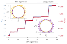
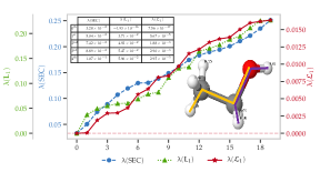
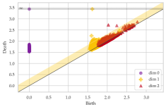
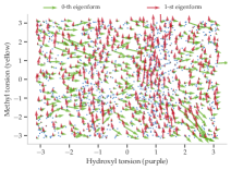
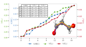
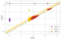
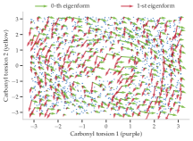
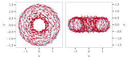
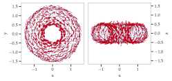
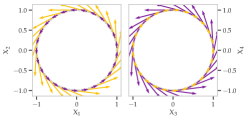
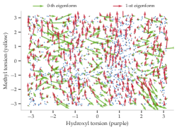
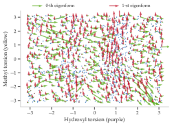
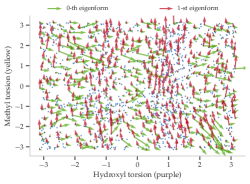
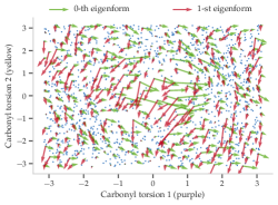
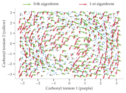
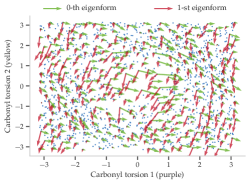
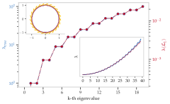
Figure 2: The first Betti number β1subscript𝛽1\beta_{1} estimation for the synthetic manifolds (first row, left to right are unit circle, torus, and flat torus), ethanol (second row), and malondialdehyde (third row) datasets. The estimated harmonic eigenforms of the synthetic datasets can be found in the inset plots of (a–c). Readers are encouraged to zoom in on these plots for better views of the vector fields and cochains. For the second and the third row, subfigures from left to right correspond to the estimated λ𝜆\lambda’s from different methods, persistent diagram of the point cloud data, and the two harmonic flows in the torsion space, respectively.

7.1 Dimension of loop space β1subscript𝛽1\beta_{1}

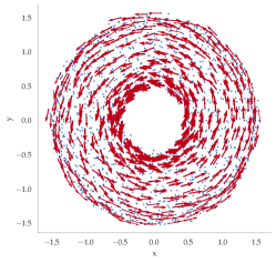
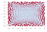
For the first Betti number β1subscript𝛽1\beta_{1}, we report the eigenvalues of Δ1subscriptΔ1\Delta_{1} estimated by SEC [BG20] (in blue), unweighted random walk Laplacian by letting 𝐖2=𝐈n2subscript𝐖2subscript𝐈subscript𝑛2\mathbf{W}_{2}=\mathbf{I}_{n_{2}} (green curve in Figure 2), and the proposed weighted 1-Laplacian 1subscript1\mathbf{\mathcal{L}}_{1} (in red). Betti numbers can also be estimated from a Persistence Diagram (PD). We present the PD with 95% confidence interval estimated from 7,000 bootstrap samples (see also [Was18] and Algorithm 4) for two chemistry datasets, i.e., the ethanol and malondialdehyde (MDA) data. All experiments are replicated at least 5 times with very similar results. The eigenvalues of the circle Δ1subscriptΔ1\Delta_{1} are λk=(k/2)2subscript𝜆𝑘superscript𝑘22\lambda_{k}=\left(\lceil k/2\rceil\right)^{2} for k=0,1,𝑘01k=0,1,\cdots. In Figure 2a we overlay the ground truth eigenvalues (blue) and the estimated eigenvalues (red) in log scale. The zeroth eigenvalue of 1ssuperscriptsubscript1𝑠\mathbf{\mathcal{L}}_{1}^{s} is close to zero, and therefore is clipped from the plot. The lower right inset plot shows the first 40 eigenvalues in linear scale. The spectrum started to diverge when k30𝑘30k\approx 30. The upper left inset plot is the original data (purple) and the estimated vector field111To estimate a vector field from a 1 co-chain, one can solve a linear system as in (S45) in Supplement I in the Least-Squares sense. (yellow arrow) corresponding to the first eigenflow, which is a harmonic flow. Figure 2b shows the computed eigenvalues of different algorithms on the synthetic torus dataset. A torus has two 1 dimensional loops. The first two eigenvalues of 𝐋1subscript𝐋1\mathbf{L}_{1} or 1subscript1\mathbf{\mathcal{L}}_{1} are close to zero, but the null space estimated by SEC has dimension 1. Inset plots show the SC2subscriptSC2\mathrm{SC}_{2} edges colored with the intensity of the first two eigenflows of 1subscript1\mathbf{\mathcal{L}}_{1}, indicating that the first eigenflow (upper left) is along the outer (bigger) circle while the second eigenvector (lower right) belongs to the inner (smaller) circle. Figure 2c shows the first fifty estimated spectrum (red) of the flat torus dataset overlaid with the ground truth (blue). The first two eigenflows correspond to harmonic flows (β1=2subscript𝛽12\beta_{1}=2). The spectrum of flat torus is piecewise constant, with half of the eigenflows for each distinct eigenvalue corresponding to gradient and the other half to curl flows. The two inset plots present the first two harmonic flows in the original space, which are shown to be parameterizing two different loops in the flat torus.

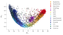
The second row of Figure 2 shows the experiment on the ethanol dataset, whose ambient and (estimated) intrinsic dimension are D=102𝐷102D=102 and d=2𝑑2d=2, respectively. The dataset is known to be a noisy non-uniformly sampled torus (see e.g., Figure S5a) with the second (inner) loop difficult to detect due to an asymmetric topological structure. The two harmonic eigenflows correspond to the relative rotations of the Hydroxyl (purple) and Methyl (yellow) functional groups as shown in the inset plot of Figure 2d. To remove the non-uniformity effect, we subsample n=1,500𝑛1500n=1,500 points that are farthest to each other. However, as shown in Figure S5a, the non-uniformity sampling effect is still drastic. For this dataset, only the spectrum of the proposed Helmholtzian 1subscript1\mathbf{\mathcal{L}}_{1} captures the correct β1=2subscript𝛽12\beta_{1}=2, which can be confirmed in Figure 2d (see Supplement J.2 for the discussion on the first 10 eigenflows); by contrast, SEC, 𝐋1subscript𝐋1\mathbf{L}_{1} and the PD estimate β1subscript𝛽1\beta_{1} to 1, 1, and more than 2, respectively. Due to the proposed triangle weight as in (3), one can successfully remove the topological noise while preserving the true signal (smaller inner loop) in the weighted 1ssuperscriptsubscript1𝑠\mathbf{\mathcal{L}}_{1}^{s}. Without the weighting function with exponential decay, the SEC and 𝐋1subscript𝐋1{\mathbf{L}}_{1} fail to detect the second inner loop thus reporting β1=1subscript𝛽11\beta_{1}=1. Apart from β1subscript𝛽1\beta_{1}, one can also obtain estimates of the two harmonic eigenflows from the first two eigenvectors of 1ssuperscriptsubscript1𝑠\mathbf{\mathcal{L}}_{1}^{s}. These two harmonic flows correspond to the two independent loops of this manifold. The first two eigenforms estimated from the eigenvectors cochain can be found in Figures S5a and S5b in Supplement. With our prior knowledge that the purple and yellow rotors parametrize the loops in the dataset, we map the two eigenforms that reside in the PCA space 𝐗𝐗{\mathbf{X}} to the torsion space using (S47) (see more discussions in Supplement I.3) as illustrated in Figure 2f. As clearly shown in the figure, the zeroth eigenform (green) aligns with the direction of increase of the Hydroxyl rotor (purple in the inset of 2d), while the first eigenform (red) matches perfectly with the derivative of Methyl rotor (yellow in the inset of 2d). Note also that one can clearly see the non-uniform sampling effect in Figure 2f. More specifically, more points are sampled when Hydroxyl torsion value is around -1 or 1 compared to other values.

The third row of Figure 2 shows the β1subscript𝛽1\beta_{1} estimation result on the MDA dataset. This dataset has similar topological structure as the ethanol dataset; that is to say, they are both non-uniformly sampled tori. The two loops are parametrized by the two Carbonyl bond torsions as illustrated in the inset plot of Figure 2g. Compared to the ethanol dataset, the MDA dataset is easier in a sense that the two loops are more symmetric to each other. However, this dataset is harder to visualize for the torus is embedded in a 4 dimensional space. A clear separation between the zeroth and the first eigenvalues of 1subscript1\mathbf{\mathcal{L}}_{1} can be seen in the estimated spectrum (Figure 2d, see also the inset table) with the help of triangle weights (3). Even though the estimated dimensions of the null space of SEC and 𝐋1subscript𝐋1{\mathbf{L}}_{1} are both two, we do not observe such clear gaps between the first two estimated eigenvalues compared to that of 1subscript1\mathbf{\mathcal{L}}_{1}. The bootstrapped PD with 95% confidence interval shows that there are at least two loops. However, statistically significant loops generated by the topological noise, which are close to the diagonal of the PD, are still visible. Similar to the ethanol dataset, we map the first two eigenforms to the two Carbonyl torsion space, as shown in Figure 2i. It confirms our prior knowledge that these two eigenforms parametrize the yellow and the purple torsions.
Refer to caption
(a)
Refer to caption
(b)
Refer to caption
(c)
Refer to caption
(d)
Refer to caption
(e)
Refer to caption
(f)
Refer to caption
(g)
Refer to caption
(h)
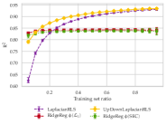
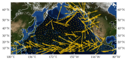
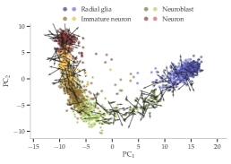
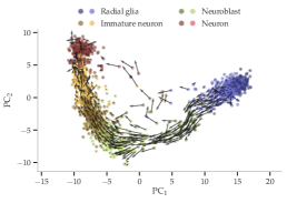
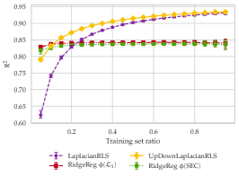
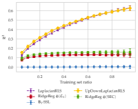
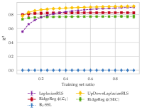
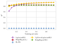
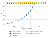
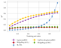
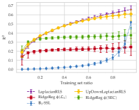
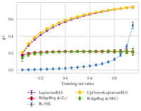
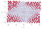
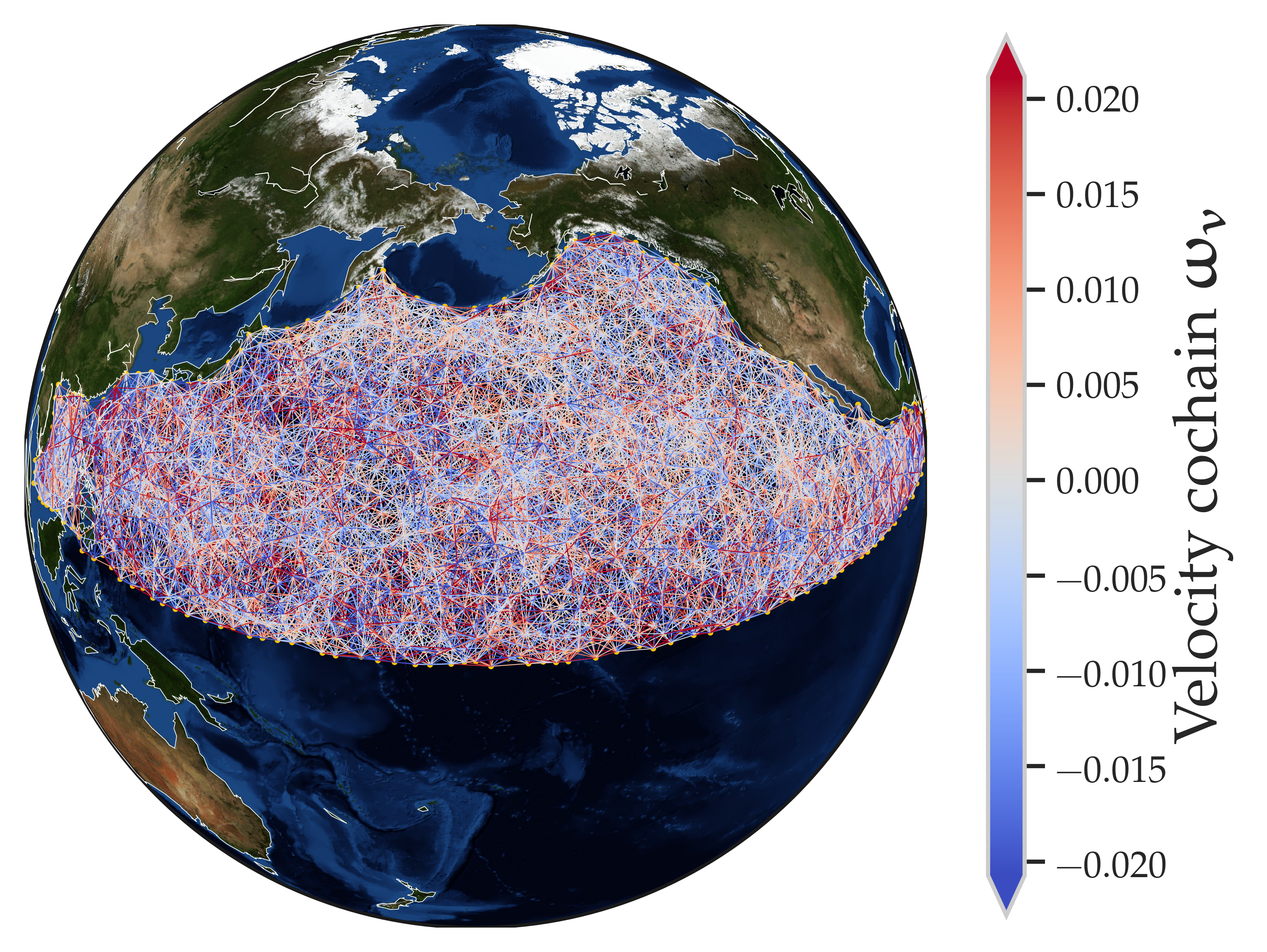
Figure 3: Edge flow SSL results for (columns from left to right) synthetic field on 2D strip, velocity field of ocean buoy, RNA velocity field of the chromaffin cells, and RNA velocity of the mouse hippocampus cell differentiation dataset. The first row is the velocity field/1-cochain overlaid on the original point cloud data, while the second row represents the R2superscript𝑅2R^{2} score of different edge flow SSL algorithms.

7.2 Edge flow prediction by semi-supervised learning

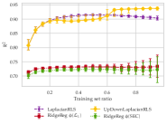
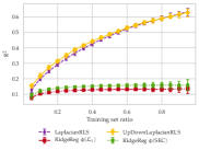
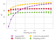
For each of the datasets in Figure 3, we construct the 1upsuperscriptsubscript1up\mathbf{\mathcal{L}}_{1}^{\rm up}, 1downsuperscriptsubscript1down\mathbf{\mathcal{L}}_{1}^{\rm down}, and the symmetrized Laplacian 1ssuperscriptsubscript1𝑠\mathbf{\mathcal{L}}_{1}^{s} as described in Section 6. We then predict the flows on a fraction of the edges (test set) from the flows of the remaining edges (training set), with edges randomly split into train and test set, for train set ratio ranges from 0.050.050.05 to 0.950.950.95. We report the coefficient of determination, R2superscript𝑅2R^{2}, as our performance metrics. The hyperparameters (all in range [105,105]superscript105superscript105[10^{-5},10^{5}]) of the LaplacianRLS (in purple) and UpDownLaplacianRLS (in yellow) on the 2D strip and ocean datasets are selected by a 5-fold cross validation (CV) for each train/test split. To reduce the computation time, the hyperparameters for the larger datasets (RNA velocity datasets) are chosen by a 5-fold CV when the train set ratio is 0.20.20.2, and are used for all the other train sample sizes. Two other baselines are ridge regression on the first 100 eigenvectors estimated by 1ssuperscriptsubscript1𝑠\mathbf{\mathcal{L}}_{1}^{s} (in red) and by SEC (in green). The 2subscript2\ell_{2} regularization parameter (in range [105,105]superscript105superscript105[10^{-5},10^{5}]) for these two baselines is chosen by a 5-fold CV for different train set size. The experiments are repeated fifty times and we report the median R2superscript𝑅2R^{2} value. The lower and upper error bars correspond to the 5th and 95th percentile of the R2superscript𝑅2R^{2} values for different train/test split, respectively.

Figure 3e shows the results of predicting the simple synthetic field shown in Figure 3a, which composed of 70% curl flow and 30% gradient flow. The results of ridge regression on the low frequency eigenvectors indicate that 100 eigenvectors estimated by either 1ssuperscriptsubscript1𝑠\mathbf{\mathcal{L}}_{1}^{s} (red) or SEC (green) are not enough even for predicting a simple field in Figure 3a.

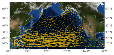
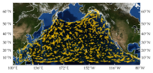
The first real dataset we used contains ocean buoy trajectories across the globe.222Data from the AOML/NOAA Drifter Data Assembly http://www.aoml.noaa.gov/envids/gld/ The ambient dimension of the data is D=3𝐷3D=3 (earth surface) and intrinsic dimension is d=2𝑑2d=2. In this paper we subsample n=1,500𝑛1500n=1,500 farthest buoys located in the North Pacific ocean. The SC2subscriptSC2\mathrm{SC}_{2} is constructed in the earth-centered, earth-fixed (ECEF) coordinate system. Supplement J.3 has more details about the data and how to preprocess the edge flow. Figure 3b shows the constructed SC2subscriptSC2\mathrm{SC}_{2} of the buoys, with edges colored by the velocity cochain ω𝜔\mathbf{\omega}. Figure 3f reports the R2superscript𝑅2R^{2} scores of the edge flow prediction. As clearly shown in the plot, higher frequency terms are needed to successfully predict the edge flow. However, this is clearly infeasible using the SEC approach as discussed in Section 5.

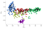
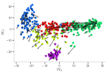
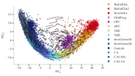
Next, we investigate the edge flow SSL on the RNA single cell sequencing manifold equipped with the RNA velocity [LMSZ+18]333All RNA datasets are from http://velocyto.org (with preprocessing codes), as shown in the third and the fourth column of Figure 3. These datasets have non-trivial manifold structures, which make the SSL problem more challenging. The Chromaffin cell differentiation dataset has n=384𝑛384n=384 and D=5𝐷5D=5, while the mouse hippocampus dataset has 18,1401814018,140 cells in total and D=10𝐷10D=10 in the PCA space. We subsample the farest n=800𝑛800n=800 cells in the mouse hippocampus while using all the cells in the chromaffin dataset. The RNA velocity fields of the Chromaffin and the mouse hippocampus datasets in the first two principal components are presented in Figure 3c and 3d, respectively. As expected, the LaplacianRLS and UpDownLaplacianRLS algorithms outperform the SSL algorithms using only low frequency terms of the estimated Δ1subscriptΔ1\Delta_{1}. Note also that compared with the SSL in the simple manifold structure in the first two columns, the UpDownLaplacianRLS for the RNA velocity data has more performance gains when the training set sizes are small.

7.3 Inverse problem: estimate the underlying velocity field from the trajectory data using SSL
Refer to caption
(a)
Refer to caption
(b)
Refer to caption
(c)
Refer to caption
(d)
Refer to caption
(e)
Refer to caption
(f)
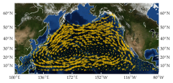
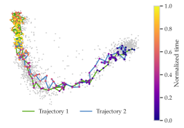
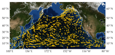
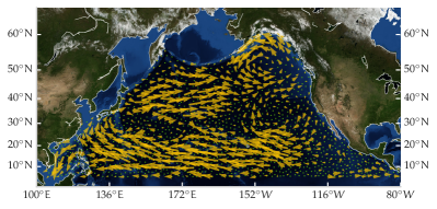
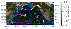
Figure 4: Results of estimating underlying velocity field from the partially observed trajectories. The first and second row are the ocean and the human glutamatergic neuron cell differentiation dataset, respectively. Columns from left to right present the observed trajectories, the estimated velocity field from a zero-padded 1-cochain, and the estimated field from the SSL interpolated 1-cochain.

One application of the Edge flow SSL is to estimate the underlying velocity field given a sparse set of observations (trajectories). A trajectory can be thought of as a partially observed 1-cochain with the value of e=(i,j)𝑒𝑖𝑗e=(i,j) constructed by counting number of times the trajectory goes from node i𝑖i to node j𝑗j (counted as negative if pass from j𝑗j to i𝑖i). We use the UpDownLaplacianRLS algorithm described in Section 6 and show the estimated fields from the interpolated 1-cochains in Figure 4. The parameters of the SSL algorithm are chosen using a 5-fold CV when test set ratio is 0.6 of all the observed edges. For comparison, we also present the velocity fields estimated by the zero-padded 1-cochains. The ocean drifter data themselves are trajectories, we sampled 20 trajectories from the dataset as shown in Figure 4a. Since we subsample the furtherest n=1,500𝑛1500n=1,500 points from the original dataset to construct the SC2=(V,E,T)subscriptSC2𝑉𝐸𝑇\mathrm{SC}_{2}=(V,E,T), the trajectories will contain points that are not in the vertex set V𝑉V. To address this issue, one can treat the vertex set V𝑉V as landmarks of the original dataset and map each point in the sampled trajectories to its nearest point in V𝑉V. The 1-cochain is then constructed from the mapped trajectories. The figure shows that we can obtain a highly interpretable velocity field that corresponds to the North pacific Gyre as in Figure 4c, compared with the estimated velocity field from the zero-padded 1-cochain (Figure 4b). The algorithm is surprisingly powerful in the sense that the sampled trajectories do not even cover the west-traveling buoys at 40 N nor the south-bounding drifters near the west coast of the U.S.

The human glutamatergic neuron cell differentiation dataset do not have the temporal information. To illustrate our method, we estimate the transition probability matrix of a Markov chain from the RNA velocity field, which is computed from a 550550550-nearest neighbor (NN) graph. We then sampled two random walk trajectories (Figure 4d) from the constructed Markov chain on the 550550550-NN graph. Note that the k𝑘k-NN graph above, which is used to estimate the RNA velocity field, can be different from the 1-skeleton of the SC2subscriptSC2\mathrm{SC}_{2} constructed in Algorithm 1. The estimated field using the UpDownLaplacianRLS in Figure 4c shows a smooth velocity field compared with the field estimated from the zero-padded 1-cochain in Figure 4b.

7.4 Edge flow smoothing
Refer to caption
(a)
Refer to caption
(b)
Refer to caption
(c)
Refer to caption
(d)
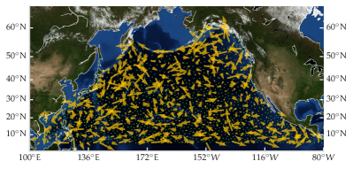
Figure 5: Edge flow smoothing on the ocean buoys velocity field dataset with different smoothing constant α𝛼\alpha.

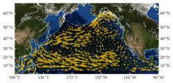
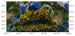
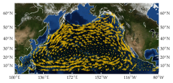
Figure 5 shows the result ω^^𝜔\hat{\mathbf{\omega}} of edge flow smoothing presented in (8). Figure 5a and 5b5d show the original and the smoothed vector fields with different smoothing parameters α𝛼\alpha, respectively. Several patterns, e.g., North Equatorial and Kuroshio currents, are visible in the original velocity field. However, a well known North Pacific current at 40superscript4040^{\circ}N is not as apparent as the aforementioned currents. By contrast, the smoothed flow with α=50𝛼50\alpha=50 makes the North Pacific Gyre visible. The model with α=5𝛼5\alpha=5 in Figure 5b corresponds to the case of “under-smoothing”, while that with α=500𝛼500\alpha=500 represents the case of “over-smoothing”. Note that the vector fields are plotted on the Mercator projection purely for visualization purposes. The SC2subscriptSC2\mathrm{SC}_{2} are constructed on the ECEF system similar as before.

8 Conclusion

The main contribution of the paper is to (\romannum1) propose an estimator of the Helmholtzian Δ1subscriptΔ1\Delta_{1} of a manifold in the form of a weighted 1-Laplacian of a two dimensional simplicial complex SC2subscriptSC2\mathrm{SC}_{2}, whose vertex set includes points sampled from a manifold. With the proposed kernel function for triangles, which is a core part of the construction of this estimator, (\romannum2) we further derive (Section 4) the infinite sample limit of 1 up-Laplacian 1upsuperscriptsubscript1up\mathbf{\mathcal{L}}_{1}^{\mathrm{up}} and 1 down-Laplacian 1downsuperscriptsubscript1down\mathbf{\mathcal{L}}_{1}^{\mathrm{down}} under the assumption that the points are sampled from a constant density supported on {\mathcal{M}}, which proves the pointwise consistency and a=14𝑎14a=\frac{1}{4} in b=1𝑏1b=1 in the Helmholtzian. The spectral consistency of the corresponding 1downsuperscriptsubscript1down\mathbf{\mathcal{L}}_{1}^{\mathrm{down}} is also shown using the spectral dependency to the well-studied graph Laplacian. (\romannum3) This work opens up avenues for the extensions of the well-studied node based Laplacian based algorithms to edge flow learning. This includes, but is not limited to, semi-supervised learning (SSL) [BNS06] on edge flows and smoothing/noise reduction for vector fields [SS18]. The classical Laplacian-type SSL and graph signal processing algorithms are thus applied to edge flow learning scenarios with the constructed weighted Helmholtzian 1ssuperscriptsubscript1𝑠\mathbf{\mathcal{L}}_{1}^{s}. Furthermore, (\romannum4) the effectiveness of the proposed weighted Helmholtzian are shown by comprehensive experiments on synthetic and real-world datasets. The proposed framework is a significant building block for new applications and algorithms in other domains of study, such as language datasets [Zhu13] with word2vec embedding [MSC+13], (multivariate) time series [GGB16], and 3D motion datasets [ABS07].

Acknowledgements

The authors acknowledge partial support from the U.S. Department of Energy’s Office of Energy Efficiency and Renewable Energy (EERE) under the Solar Energy Technologies Office Award Number DE-EE0008563 (M.M. and Y.C.), from the NSF DMS PD 08-1269 (M.M. and Y.C.), and an ARO MURI (I.G.K.). Part of this research was performed while the three authors were visiting the Institute for Pure and Applied Mathematics (IPAM), which is supported by the National Science Foundation (Grant No. DMS-1925919). In addition, M.M. gratefully acknowledges an IPAM Simons Fellowship. This work was facilitated through the use of advanced computational, storage, and networking infrastructure provided by the Hyak supercomputer system and funded by the STF at the University of Washington. M.M. and Y.C. thank the Tkatchenko and Pfaendtner labs and in particular to Stefan Chmiela and Chris Fu for providing the molecular dynamics data and for many hours of brainstorming and advice, some of which took place at IPAM.

Disclaimer

The views expressed herein do not necessarily represent the views of the U.S. Department of Energy or the United States Government.

References

  • [ABS07] Saad Ali, Arslan Basharat, and Mubarak Shah. Chaotic Invariants for Human Action Recognition. In 2007 IEEE 11th International Conference on Computer Vision, pages 1–8, October 2007.
  • [AFW10] Douglas Arnold, Richard Falk, and Ragnar Winther. Finite element exterior calculus: From Hodge theory to numerical stability. Bulletin of the American Mathematical Society, 47(2):281–354, 2010.
  • [BG20] Tyrus Berry and Dimitrios Giannakis. Spectral exterior calculus. Communications on Pure and Applied Mathematics, 73(4):689–770, 2020.
  • [BN07] Mikhail Belkin and Partha Niyogi. Convergence of laplacian eigenmaps. In B. Schölkopf, J. C. Platt, and T. Hoffman, editors, Advances in Neural Information Processing Systems 19, pages 129–136. MIT Press, 2007.
  • [BNPB13] H. Bhatia, G. Norgard, V. Pascucci, and P. Bremer. The Helmholtz-Hodge Decomposition—A Survey. IEEE Transactions on Visualization and Computer Graphics, 19(8):1386–1404, August 2013.
  • [BNS06] Mikhail Belkin, Partha Niyogi, and Vikas Sindhwani. Manifold regularization: A geometric framework for learning from labeled and unlabeled examples. Journal of machine learning research, 7(Nov):2399–2434, 2006.
  • [BS19] Tyrus Berry and Timothy Sauer. Consistent manifold representation for topological data analysis. Foundations of Data Science, 1(1):1, 2019.
  • [Chu96] Fan Chung. Spectral Graph Theory, volume 92 of CBMS Regional Conference Series in Mathematics. American Mathematical Society, December 1996.
  • [CL06] Ronald R. Coifman and Stéphane Lafon. Diffusion maps. Applied and Computational Harmonic Analysis, 21(1):5–30, July 2006.
  • [Cle17] Jeanne N. Clelland. From Frenet to Cartan: The Method of Moving Frames, volume 178. American Mathematical Soc., 2017.
  • [CLM13] Guangliang Chen, Anna V. Little, and Mauro Maggioni. Multi-Resolution Geometric Analysis for Data in High Dimensions, pages 259–285. Birkhäuser Boston, Boston, 2013.
  • [CM17] Frédéric Chazal and Bertrand Michel. An introduction to Topological Data Analysis: Fundamental and practical aspects for data scientists. arXiv:1710.04019 [cs, math, stat], October 2017.
  • [CMOP11] Ozan Candogan, Ishai Menache, Asuman Ozdaglar, and Pablo A. Parrilo. Flows and Decompositions of Games: Harmonic and Potential Games. Mathematics of Operations Research, 36(3):474–503, August 2011.
  • [Col06] Bruno Colbois. Spectral Theory and Geometry. pp.34:cel–00392158, 2006.
  • [CTS+17] Stefan Chmiela, Alexandre Tkatchenko, Huziel E Sauceda, Igor Poltavsky, Kristof T Schütt, and Klaus-Robert Müller. Machine learning of accurate energy-conserving molecular force fields. Science advances, 3(5):e1603015, 2017.
  • [DFW13] Tamal K. Dey, Fengtao Fan, and Yusu Wang. Graph Induced Complex on Point Data. arXiv:1304.0662 [cs, math], April 2013.
  • [DKT08] Mathieu Desbrun, Eva Kanso, and Yiying Tong. Discrete Differential Forms for Computational Modeling. In Alexander I. Bobenko, John M. Sullivan, Peter Schröder, and Günter M. Ziegler, editors, Discrete Differential Geometry, Oberwolfach Seminars, pages 287–324. Birkhäuser, Basel, 2008.
  • [DM95] Józef Dodziuk and Jeffrey McGowan. The Spectrum of the Hodge Laplacian for a Degenerating Family of Hyperbolic Three Manifolds. Transactions of the American Mathematical Society, 347(6):1981–1995, 1995.
  • [Dod76] Jozef Dodziuk. Finite-Difference Approach to the Hodge Theory of Harmonic Forms. American Journal of Mathematics, 98(1):79–104, 1976.
  • [Eck44] Beno Eckmann. Harmonische Funktionen und Randwertaufgaben in einem Komplex. Commentarii mathematici Helvetici, 17:240–255, 1944.
  • [FP15] Gary Froyland and Kathrin Padberg-Gehle. A rough-and-ready cluster-based approach for extracting finite-time coherent sets from sparse and incomplete trajectory data. Chaos: An Interdisciplinary Journal of Nonlinear Science, 25(8):087406, July 2015.
  • [GGB16] Chad Giusti, Robert Ghrist, and Danielle S. Bassett. Two’s company, three (or more) is a simplex. Journal of Computational Neuroscience, 41(1):1–14, August 2016.
  • [GP10] Leo J. Grady and Jonathan Polimeni. Discrete Calculus: Applied Analysis on Graphs for Computational Science. Springer-Verlag, London, 2010.
  • [GR13] Chris Godsil and Gordon F. Royle. Algebraic Graph Theory. Springer Science & Business Media, December 2013.
  • [HJ13] Danijela Horak and Jürgen Jost. Spectra of combinatorial Laplace operators on simplicial complexes. Advances in Mathematics, 244:303–336, September 2013.
  • [JLYY11] Xiaoye Jiang, Lek-Heng Lim, Yuan Yao, and Yinyu Ye. Statistical ranking and combinatorial Hodge theory. Mathematical Programming, 127(1):203–244, March 2011.
  • [JMM17] Dominique Joncas, Marina Meila, and James McQueen. Improved graph laplacian via geometric Self-Consistency. In I Guyon, U V Luxburg, S Bengio, H Wallach, R Fergus, S Vishwanathan, and R Garnett, editors, Advances in Neural Information Processing Systems 30, pages 4457–4466. Curran Associates, Inc., 2017.
  • [JSSB19] Junteng Jia, Michael T. Schaub, Santiago Segarra, and Austin R. Benson. Graph-based Semi-Supervised & Active Learning for Edge Flows. In KDD, 2019.
  • [KS13] Michael Kerber and R. Sharathkumar. Approximate Čech Complex in Low and High Dimensions. In Leizhen Cai, Siu-Wing Cheng, and Tak-Wah Lam, editors, Algorithms and Computation, Lecture Notes in Computer Science, pages 666–676, Berlin, Heidelberg, 2013. Springer.
  • [Lee06] John M. Lee. Riemannian Manifolds: An Introduction to Curvature, volume 176. Springer Science & Business Media, 2006.
  • [Lim20] Lek-Heng Lim. Hodge laplacians on graphs. Siam Review, 62(3):685–715, 2020.
  • [LMSZ+18] Gioele La Manno, Ruslan Soldatov, Amit Zeisel, Emelie Braun, Hannah Hochgerner, Viktor Petukhov, Katja Lidschreiber, Maria E. Kastriti, Peter Lönnerberg, and Alessandro Furlan. RNA velocity of single cells. Nature, 560(7719):494–498, 2018.
  • [LPS15] Siu Kwan Lam, Antoine Pitrou, and Stanley Seibert. Numba: A LLVM-based Python JIT compiler. In Proceedings of the Second Workshop on the LLVM Compiler Infrastructure in HPC, LLVM ’15, pages 1–6, Austin, Texas, November 2015. Association for Computing Machinery.
  • [LSW09] Chuanjiang Luo, Issam Safa, and Yusu Wang. Approximating gradients for meshes and point clouds via diffusion metric. In Computer Graphics Forum, volume 28, pages 1497–1508. Wiley Online Library, 2009.
  • [MBGY14] Clément Maria, Jean-Daniel Boissonnat, Marc Glisse, and Mariette Yvinec. The gudhi library: Simplicial complexes and persistent homology. In International Congress on Mathematical Software, pages 167–174. Springer, 2014.
  • [MS16] Sayan Mukherjee and John Steenbergen. Random walks on simplicial complexes and harmonics. Random structures & algorithms, 49(2):379–405, 2016.
  • [MSC+13] Tomas Mikolov, Ilya Sutskever, Kai Chen, Greg S Corrado, and Jeff Dean. Distributed Representations of Words and Phrases and their Compositionality. In C. J. C. Burges, L. Bottou, M. Welling, Z. Ghahramani, and K. Q. Weinberger, editors, Advances in Neural Information Processing Systems 26, pages 3111–3119. Curran Associates, Inc., 2013.
  • [MW06] Sayan Mukherjee and Qiang Wu. Estimation of gradients and coordinate covariation in classification. Journal of Machine Learning Research, 7(Nov):2481–2514, 2006.
  • [NLCK06] Boaz Nadler, Stéphane Lafon, Ronald R. Coifman, and Ioannis G. Kevrekidis. Diffusion maps, spectral clustering and reaction coordinates of dynamical systems. Applied and Computational Harmonic Analysis, 21(1):113–127, 2006.
  • [OFK+18] Antonio Ortega, Pascal Frossard, Jelena Kovačević, José M. F. Moura, and Pierre Vandergheynst. Graph Signal Processing: Overview, Challenges, and Applications. Proceedings of the IEEE, 106(5):808–828, May 2018.
  • [OPT+17] Nina Otter, Mason A. Porter, Ulrike Tillmann, Peter Grindrod, and Heather A. Harrington. A roadmap for the computation of persistent homology. EPJ Data Science, 6(1):17, December 2017.
  • [Pos09] Olaf Post. First Order Approach and Index Theorems for Discrete and Metric Graphs. Annales Henri Poincaré, 10(5):823–866, August 2009.
  • [PR17] Ori Parzanchevski and Ron Rosenthal. Simplicial complexes: Spectrum, homology and random walks. Random Structures & Algorithms, 50(2):225–261, March 2017.
  • [SBH+20] Michael T. Schaub, Austin R. Benson, Paul Horn, Gabor Lippner, and Ali Jadbabaie. Random walks on simplicial complexes and the normalized Hodge 1-Laplacian. SIAM Review, 62(2):353–391, 2020.
  • [She13] Donald R. Sheehy. Linear-size approximations to the Vietoris–Rips filtration. Discrete & Computational Geometry, 49(4):778–796, 2013.
  • [Sin06] A. Singer. From graph to manifold Laplacian: The convergence rate. Applied and Computational Harmonic Analysis, 21(1):128–134, July 2006.
  • [SS18] M. T. Schaub and S. Segarra. Flow Smoothing And Denoising: Graph Signal Processing In The Edge-Space. In 2018 IEEE Global Conference on Signal and Information Processing (GlobalSIP), pages 735–739, November 2018.
  • [SW11] Amit Singer and Hau-tieng Wu. Vector Diffusion Maps and the Connection Laplacian. arXiv:1102.0075 [math, stat], January 2011.
  • [THJ10] Daniel Ting, Ling Huang, and Michael Jordan. An Analysis of the Convergence of Graph Laplacians. In Proceedings of the 27th International Conference on Machine Learning (ICML), 2010.
  • [Was18] Larry Wasserman. Topological data analysis. Annual Review of Statistics and Its Application, 5:501–532, 2018.
  • [Whi05] Hassler Whitney. Geometric Integration Theory. Dover Publications, Mineola, N.Y, December 2005.
  • [ZG02] Xiaojin Zhu and Zoubin Ghahramani. Learning from labeled and unlabeled data with label propagation. 2002.
  • [ZGL03] Xiaojin Zhu, Zoubin Ghahramani, and John Lafferty. Semi-supervised learning using Gaussian fields and harmonic functions. In Proceedings of the Twentieth International Conference on International Conference on Machine Learning, ICML’03, pages 912–919, Washington, DC, USA, August 2003. AAAI Press.
  • [Zhu13] Xiaojin Zhu. Persistent Homology: An Introduction and a New Text Representation for Natural Language Processing. In Twenty-Third International Joint Conference on Artificial Intelligence, June 2013.

Supplementary Material of
Helmholtzian Eigenmap: Topological feature discovery & edge flow learning from point cloud data

Table of Contents

\startcontents

[appendix] \printcontents[appendix]l1

Appendix A Notational table

Table S1: Notational table
Matrix operation
𝐌𝐌\mathbf{M} Matrix
𝐦isubscript𝐦𝑖\mathbf{m}_{i} Vector represents the i𝑖i-th row of 𝐌𝐌\mathbf{M}
𝐦:,jTsuperscriptsubscript𝐦:𝑗𝑇\mathbf{m}_{:,j}^{T} Vector represents the j𝑗j-th column of 𝐌𝐌\mathbf{M}
mijsubscript𝑚𝑖𝑗m_{ij} Scalar represents ij𝑖𝑗ij-th element of 𝐌𝐌\mathbf{M}
[𝐌]ijsubscriptdelimited-[]𝐌𝑖𝑗[\mathbf{M}]_{ij} Scalar, alternative notation for mijsubscript𝑚𝑖𝑗m_{ij}
𝐌[α,β]𝐌𝛼𝛽\mathbf{M}[\alpha,\beta] Submatrix of 𝐌𝐌\mathbf{M} of index sets α,β𝛼𝛽\alpha,\beta
𝐯𝐯\mathbf{v} Column vecor
visubscript𝑣𝑖v_{i} Scalar represents i𝑖i-th element of vecor 𝐯𝐯\mathbf{v}
[𝐯]isubscriptdelimited-[]𝐯𝑖[\mathbf{v}]_{i} Scalar, alternative notation for visubscript𝑣𝑖v_{i}
Scalars
n𝑛n Number of samples (nodes) (=n0)absentsubscript𝑛0(=n_{0})
nksubscript𝑛𝑘n_{k} Dimension of k𝑘k co-chain (=|Σk|)absentsubscriptΣ𝑘(=|\Sigma_{k}|)
d𝑑d Intrinsic dimension
δ𝛿\delta Bandwidth parameter for 𝐋𝐋\mathbf{L}
ε𝜀\varepsilon Bandwidth parameter for 𝐖2subscript𝐖2\mathbf{W}_{2}
Vectors & Matrices
𝐗𝐗\mathbf{X} Data matrix
𝐱isubscript𝐱𝑖\mathbf{x}_{i} Point i𝑖i in ambient space
𝐁ksubscript𝐁𝑘\mathbf{B}_{k} Boundary operator of k𝑘k chain
𝐋𝐋\mathbf{L} Graph Laplacian
𝐋ksubscript𝐋𝑘\mathbf{L}_{k} k𝑘k unnormalized Hodge Laplacian
𝐰ksubscript𝐰𝑘\mathbf{w}_{k} nkabsentsuperscriptsubscript𝑛𝑘\in\mathbb{R}^{n_{k}}, weights of k𝑘k (co)chain
𝐖ksubscript𝐖𝑘\mathbf{W}_{k} =diag(𝐰k)absentdiagsubscript𝐰𝑘=\mathrm{diag}(\mathbf{w}_{k})
ksubscript𝑘\mathbf{\mathcal{L}}_{k} k𝑘k random walk Hodge Laplacian
kssuperscriptsubscript𝑘𝑠\mathbf{\mathcal{L}}_{k}^{s} k𝑘k symmetrized Hodge Laplacian
𝐈nsubscript𝐈𝑛\mathbf{I}_{n} Identity matrix n×nabsentsuperscript𝑛𝑛\in\mathbb{R}^{n\times n}
𝟏nsubscript1𝑛\mathbf{1}_{n} All one vecor nabsentsuperscript𝑛\in\mathbb{R}^{n}
𝟏Ssubscript1𝑆\mathbf{1}_{S} [𝟏S]i=1subscriptdelimited-[]subscript1𝑆𝑖1[\mathbf{1}_{S}]_{i}=1 if iS𝑖𝑆i\in S 0 otherwise
𝟎nsubscript0𝑛\mathbf{0}_{n} All zero vecor nabsentsuperscript𝑛\in\mathbb{R}^{n}
Miscellaneous
ΣksubscriptΣ𝑘\Sigma_{k} Set of k𝑘k-simplices
V=Σ0𝑉subscriptΣ0V=\Sigma_{0} Set of nodes
E=Σ1𝐸subscriptΣ1E=\Sigma_{1} Set of edges
T=Σ2𝑇subscriptΣ2T=\Sigma_{2} Set of triangles
SCsubscriptSC\mathrm{SC}_{\ell} =(Σk)k=0=(Σ0,Σ1,,Σ)absentsuperscriptsubscriptsubscriptΣ𝑘𝑘0subscriptΣ0subscriptΣ1subscriptΣ=(\Sigma_{k})_{k=0}^{\ell}=(\Sigma_{0},\Sigma_{1},\cdots,\Sigma_{\ell})
simplicial complex up to dimension \ell
G(V,E)𝐺𝑉𝐸G(V,E) Graph with vertex set V𝑉V and edge set E𝐸E
=SC1=(Σ0,Σ1)absentsubscriptSC1subscriptΣ0subscriptΣ1=\mathrm{SC}_{1}=(\Sigma_{0},\Sigma_{1})
\mathcal{M} Data manifold
[s]delimited-[]𝑠[s] Set {1,,s}1𝑠\{1,\cdots,s\}
ϵπsubscriptitalic-ϵ𝜋\epsilon_{\pi} Levi-Civita symbol for permutation π𝜋\pi
𝖽𝖽\mathsf{d} Exterior derivative
δδ\updelta Co-differential operator

Appendix B Pseudocodes

Input : Set of k1𝑘1k-1 and k𝑘k simplices Σk1subscriptΣ𝑘1\Sigma_{k-1}, ΣksubscriptΣ𝑘\Sigma_{k}
1 𝐁k𝟎nk1𝟎nknk1×nksubscript𝐁𝑘subscript0subscript𝑛𝑘1superscriptsubscript0subscript𝑛𝑘topsuperscriptsubscript𝑛𝑘1subscript𝑛𝑘\mathbf{B}_{k}\leftarrow\mathbf{0}_{n_{k-1}}\mathbf{0}_{n_{k}}^{\top}\in\mathbb{R}^{n_{k-1}\times n_{k}}
2 for every σk1Σk1subscript𝜎𝑘1subscriptΣ𝑘1\sigma_{k-1}\in\Sigma_{k-1} do
3       for every σkΣksubscript𝜎𝑘subscriptΣ𝑘\sigma_{k}\in\Sigma_{k} do
4             if σk1subscript𝜎𝑘1\sigma_{k-1} is a face of σksubscript𝜎𝑘\sigma_{k} then
                   [𝐁k]σk1,σkϵij,i0ij^iksubscriptdelimited-[]subscript𝐁𝑘subscript𝜎𝑘1subscript𝜎𝑘subscriptitalic-ϵsubscript𝑖𝑗subscript𝑖0^subscript𝑖𝑗subscript𝑖𝑘[\mathbf{B}_{k}]_{\sigma_{k-1},\sigma_{k}}\leftarrow\epsilon_{i_{j},i_{0}\cdots\hat{i_{j}}\cdots i_{k}} \triangleright See (S3).
5                  
6             else
7                  [𝐁k]σk1,σk0subscriptdelimited-[]subscript𝐁𝑘subscript𝜎𝑘1subscript𝜎𝑘0[\mathbf{B}_{k}]_{\sigma_{k-1},\sigma_{k}}\leftarrow 0
8             end if
9            
10       end for
11      
12 end for
13
Return : Boundary map for k𝑘k-chain 𝐁ksubscript𝐁𝑘\mathbf{B}_{k}
Algorithm 2 BoundaryMap
Input : Data matrix 𝐗n×D𝐗superscript𝑛𝐷{\mathbf{X}}\in\mathbb{R}^{n\times D}, radius max_dist δ𝛿\delta, max_dim k𝑘k
1 Build graph G(V,E)𝐺𝑉𝐸G(V,E) with V=[n]𝑉delimited-[]𝑛V=[n] and E={(i,j)V2:𝐱i𝐱j<δ}E=\{(i,j)\in V^{2}:\|{\mathbf{x}}_{i}-\|{\mathbf{x}}_{j}\|<\delta\}
2 for =2k2𝑘\ell=2\to k do
       Σ={(i0,,i)V:eEe((i0,,i)2)}subscriptΣconditional-setsubscript𝑖0subscript𝑖superscript𝑉𝑒𝐸for-all𝑒binomialsubscript𝑖0subscript𝑖2\Sigma_{\ell}=\{(i_{0},\cdots,i_{\ell})\in V^{\ell}:e\in E\,\forall\,e\in\binom{(i_{0},\cdots,i_{\ell})}{2}\} \triangleright Clique complex of G𝐺G
3      
4 end for
Return : VR complex SCk=(V,E,,Σk)subscriptSC𝑘𝑉𝐸subscriptΣ𝑘\mathrm{SC}_{k}=(V,E,\cdots,\Sigma_{k})
Algorithm 3 VRComplex
Input : Data matrix 𝐗n×D𝐗superscript𝑛𝐷{\mathbf{X}}\in\mathbb{R}^{n\times D}, max_dim k𝑘k, num_bootstrap_samples B𝐵B, significance level α𝛼\alpha
1 Compute persistent diagram 𝒫PD(𝐗,k)𝒫PD𝐗𝑘\mathcal{P}\leftarrow\text{\sc PD}({\mathbf{X}},k)
2 for i=1B𝑖1𝐵i=1\to B do
3       Sample [𝐱~i]i=1nsuperscriptsubscriptdelimited-[]subscript~𝐱𝑖𝑖1𝑛[\tilde{\mathbf{x}}_{i}]_{i=1}^{n} with replacement from 𝐗𝐗{\mathbf{X}}
4       Bootstrapped PD 𝒫~iPD(𝐗~,k)subscript~𝒫𝑖PD~𝐗𝑘\tilde{\mathcal{P}}_{i}\leftarrow\text{\sc PD}(\tilde{\mathbf{X}},k)
5       for =0k0𝑘\ell=0\to k do
6             𝔇iBottleneckDist(𝒫,𝒫~i,)subscriptsuperscript𝔇𝑖BottleneckDist𝒫subscript~𝒫𝑖\mathfrak{D}^{\ell}_{i}\leftarrow\text{\sc BottleneckDist}(\mathcal{P},\tilde{\mathcal{P}}_{i},\ell)
7       end for
8      
9 end for
10for =0k0𝑘\ell=0\to k do
11       bαPercentile(𝔇i,1α)superscriptsubscript𝑏𝛼Percentilesubscriptsuperscript𝔇𝑖1𝛼b_{\alpha}^{\ell}\leftarrow\text{\sc Percentile}(\mathfrak{D}^{\ell}_{i},1-\alpha)
12 end for
Return : Confidence band {bα}=0ksuperscriptsubscriptsuperscriptsubscript𝑏𝛼0𝑘\{b_{\alpha}^{\ell}\}_{\ell=0}^{k}
Algorithm 4 BootstrapPD

Appendix C Rigorous definitions

First we define the Levi-Civita notation and permutation parity. This is useful for the definition of boundary operator 𝐁ksubscript𝐁𝑘{\mathbf{B}}_{k}.

Definition S1 (Permutation parity).

Given a finite set {j0,j1,,jk}subscript𝑗0subscript𝑗1subscript𝑗𝑘\{j_{0},j_{1},\cdots,j_{k}\} with k1𝑘1k\geq 1 and j<jmsubscript𝑗subscript𝑗𝑚j_{\ell}<j_{m} if <m𝑚\ell<m, the parity of a permutation ς({j0,,jk})={i0,i1,,ik}𝜍subscript𝑗0subscript𝑗𝑘subscript𝑖0subscript𝑖1subscript𝑖𝑘\varsigma(\{j_{0},\cdots,j_{k}\})=\{i_{0},i_{1},\cdots,i_{k}\} is defined to be

ϵi0,,ik=1N(ς).subscriptitalic-ϵsubscript𝑖0subscript𝑖𝑘superscript1𝑁𝜍\epsilon_{i_{0},\cdots,i_{k}}=-1^{N(\varsigma)}. (S1)

Here N(ς)𝑁𝜍N(\varsigma) is the inversion number of ς𝜍\varsigma. The inversion number is the cardinality of the inversion set, i.e., N(ς)=#{(,m):i>im if <m}𝑁𝜍#conditional-set𝑚subscript𝑖subscript𝑖𝑚 if 𝑚N(\varsigma)=\#\{(\ell,m):i_{\ell}>i_{m}\text{ if }\ell<m\}. We say ς𝜍\varsigma is an even permutation if ϵi0,,ik=1subscriptitalic-ϵsubscript𝑖0subscript𝑖𝑘1\epsilon_{i_{0},\cdots,i_{k}}=1 and an odd permutation otherwise.

Remark.

When k=1𝑘1k=1, the Levi-Civita symbol is

ϵij={+1if (i,j)=(1,2),1if (i,j)=(2,1).subscriptitalic-ϵ𝑖𝑗cases1if 𝑖𝑗121if 𝑖𝑗21\epsilon_{ij}=\begin{cases}+1\,&\text{if }\,(i,j)=(1,2),\\ -1\,&\text{if }\,(i,j)=(2,1).\end{cases}

For k=2𝑘2k=2, the Levi-Civita symbol is

ϵijk={+1if (i,j,k){(1,2,3),(2,3,1),(3,1,2)},1if (i,j,k){(3,2,1),(1,3,2),(2,1,3)}.subscriptitalic-ϵ𝑖𝑗𝑘cases1if 𝑖𝑗𝑘1232313121if 𝑖𝑗𝑘321132213\epsilon_{ijk}=\begin{cases}+1\,&\text{if }\,(i,j,k)\in\{(1,2,3),(2,3,1),(3,1,2)\},\\ -1\,&\text{if }\,(i,j,k)\in\{(3,2,1),(1,3,2),(2,1,3)\}.\end{cases}

With this in hand, one can define the boundary map as follows.

Definition S2 (Boundary map & boundary matrix).

Let i0ij^iki0,,ij1,ij+1,,iksubscript𝑖0^subscript𝑖𝑗subscript𝑖𝑘subscript𝑖0subscript𝑖𝑗1subscript𝑖𝑗1subscript𝑖𝑘i_{0}\cdots\hat{i_{j}}\cdots i_{k}\coloneqq i_{0},\cdots,i_{j-1},i_{j+1},\cdots,i_{k}, and i0ijˇiksubscript𝑖0ˇsubscript𝑖𝑗subscript𝑖𝑘i_{0}\cdots\check{i_{j}}\cdots i_{k} denote ijsubscript𝑖𝑗i_{j} insert into i0,,iksubscript𝑖0subscript𝑖𝑘i_{0},\cdots,i_{k} with proper order, we define a boundary map (operator) k:𝒞k𝒞k1:subscript𝑘subscript𝒞𝑘subscript𝒞𝑘1\mathcal{B}_{k}:\mathcal{C}_{k}\to\mathcal{C}_{k-1}, which maps a simplex to its face, by

k([i0,,ik])=j=0k(1)j[i0ij^ik]=j=0kϵij,i0ij^ik[i0ij^ik].subscript𝑘subscript𝑖0subscript𝑖𝑘superscriptsubscript𝑗0𝑘superscript1𝑗delimited-[]subscript𝑖0^subscript𝑖𝑗subscript𝑖𝑘superscriptsubscript𝑗0𝑘subscriptitalic-ϵsubscript𝑖𝑗subscript𝑖0^subscript𝑖𝑗subscript𝑖𝑘delimited-[]subscript𝑖0^subscript𝑖𝑗subscript𝑖𝑘\mathcal{B}_{k}([i_{0},\cdots,i_{k}])=\sum_{j=0}^{k}(-1)^{j}[i_{0}\cdots\hat{i_{j}}\cdots i_{k}]=\sum_{j=0}^{k}\epsilon_{i_{j},i_{0}\cdots\hat{i_{j}}\cdots i_{k}}[i_{0}\cdots\hat{i_{j}}\cdots i_{k}]. (S2)

Here ij,i0ij^ikij,i0,,ij1,ij+1,,ikformulae-sequencesubscript𝑖𝑗subscript𝑖0^subscript𝑖𝑗subscript𝑖𝑘subscript𝑖𝑗subscript𝑖0subscript𝑖𝑗1subscript𝑖𝑗1subscript𝑖𝑘i_{j},i_{0}\cdots\hat{i_{j}}\cdots i_{k}\coloneqq i_{j},i_{0},\cdots,i_{j-1},i_{j+1},\cdots,i_{k}.

The corresponding boundary matrix 𝐁k{0,±1}nk1×nksubscript𝐁𝑘superscript0plus-or-minus1subscript𝑛𝑘1subscript𝑛𝑘\mathbf{B}_{k}\in\{0,\pm 1\}^{n_{k-1}\times n_{k}} can be defined as follows.

(𝐁k)σk1,σk{ϵij,i0ij^ikif σk=[i0,,ik],σk1=[i0ij^ik],0otherwise.subscriptsubscript𝐁𝑘subscript𝜎𝑘1subscript𝜎𝑘casessubscriptitalic-ϵsubscript𝑖𝑗subscript𝑖0^subscript𝑖𝑗subscript𝑖𝑘formulae-sequenceif subscript𝜎𝑘subscript𝑖0subscript𝑖𝑘subscript𝜎𝑘1delimited-[]subscript𝑖0^subscript𝑖𝑗subscript𝑖𝑘0otherwise.(\mathbf{B}_{k})_{\sigma_{k-1},\sigma_{k}}\begin{cases}\epsilon_{i_{j},i_{0}\cdots\hat{i_{j}}\cdots i_{k}}\,&\text{if }\,\sigma_{k}=[i_{0},\cdots,i_{k}],\,\,\sigma_{k-1}=[i_{0}\cdots\hat{i_{j}}\cdots i_{k}],\\ 0\,&\text{otherwise.}\end{cases} (S3)

(𝐁k)σk1,σksubscriptsubscript𝐁𝑘subscript𝜎𝑘1subscript𝜎𝑘(\mathbf{B}_{k})_{\sigma_{k-1},\sigma_{k}} represents the orientation of σk1subscript𝜎𝑘1\sigma_{k-1} as a face of σksubscript𝜎𝑘\sigma_{k}, or equals 0 when the two are not adjacent.

Example.

For the simplicial complex SC2subscriptSC2\mathrm{SC}_{2} in Figure S1, the corresponding 𝐁1subscript𝐁1{\mathbf{B}}_{1} is in Table S3 while 𝐁2subscript𝐁2{\mathbf{B}}_{2} is in Table S2.

Down Helmholtzian 1downsuperscriptsubscript1down\mathbf{\mathcal{L}}_{1}^{\mathrm{down}}Graph Laplacian 0subscript0\mathbf{\mathcal{L}}_{0}Δ1down=𝖽0δ1superscriptsubscriptΔ1downsubscript𝖽0subscriptδ1\Delta_{1}^{\mathrm{down}}=\mathsf{d}_{0}\updelta_{1}Δ0=δ1𝖽0subscriptΔ0subscriptδ1subscript𝖽0\Delta_{0}=\updelta_{1}\mathsf{d}_{0}
Lemma S16
[DM95, Col06]
Proposition S17111222333444555666777888999101010
Figure S1: Illustration of a SC2=(Σ0,Σ1,Σ2)subscriptSC2subscriptΣ0subscriptΣ1subscriptΣ2\mathrm{SC}_{2}=(\Sigma_{0},\Sigma_{1},\Sigma_{2}), shaded region denotes that the triangle tΣ2𝑡subscriptΣ2t\in\Sigma_{2}.
(1, 2, 3)
(1, 2) 1
(1, 3) -1
(1, 4) 0
(2, 3) 1
(3, 4) 0
(3, 5) 0
(5, 6) 0
(5, 8) 0
(6, 7) 0
(7, 8) 0
Table S2: 𝐁2subscript𝐁2{\mathbf{B}}_{2} of SC2subscriptSC2\mathrm{SC}_{2}
(1, 2) (1, 3) (1, 4) (2, 3) (3, 4) (3, 5) (5, 6) (5, 8) (6, 7) (7, 8) (9, 10)
1 1 1 1 0 0 0 0 0 0 0 0
2 -1 0 0 1 0 0 0 0 0 0 0
3 0 -1 0 -1 1 1 0 0 0 0 0
4 0 0 -1 0 -1 0 0 0 0 0 0
5 0 0 0 0 0 -1 1 1 0 0 0
6 0 0 0 0 0 0 -1 0 1 0 0
7 0 0 0 0 0 0 0 0 -1 1 0
8 0 0 0 0 0 0 0 -1 0 -1 0
9 0 0 0 0 0 0 0 0 0 0 1
10 0 0 0 0 0 0 0 0 0 0 -1
Table S3: Boundary matrix 𝐁1subscript𝐁1{\mathbf{B}}_{1} (incident matrix) of SC2subscriptSC2\mathrm{SC}_{2} in Figure S1.

In this example, triangle is not always filled, e.g., [1,3,4]Σ2134subscriptΣ2[1,3,4]\notin\Sigma_{2}. However, for the construction of VR complex described in Algorithm 1, every triangle in SC2subscriptSC2\mathrm{SC}_{2} is filled.

Below we provide the definition of the Hodge star operator and 𝖽𝖽\mathsf{d}, δδ\updelta.

Definition S3 (Hodge star).

Hodge star on 1 form (dual of basis function) is defined as follow,

(𝖽si1𝖽sik)=ϵIJ𝖽sj1𝖽sjdk\star(\mathsf{d}s_{i_{1}}\wedge\cdots\wedge\mathsf{d}s_{i_{k}})=\epsilon_{IJ}\mathsf{d}s_{j_{1}}\wedge\cdots\wedge\mathsf{d}s_{j_{d-k}} (S4)

Here J={j1,jdk}𝐽subscript𝑗1subscript𝑗𝑑𝑘J=\{j_{1}\cdots,j_{d-k}\} is the (ordered) complement of I={i1,,ik}𝐼subscript𝑖1subscript𝑖𝑘I=\{i_{1},\cdots,i_{k}\}. E.g., if I={1,5}𝐼15I=\{1,5\} in d=7𝑑7d=7 dimensional space, we have J={2,3,4,6,7}𝐽23467J=\{2,3,4,6,7\}. ϵIJsubscriptitalic-ϵ𝐼𝐽\epsilon_{IJ} is the Levi-Civita symbol of the permutation IJ={i1ik,j1,jnk}𝐼𝐽subscript𝑖1subscript𝑖𝑘subscript𝑗1subscript𝑗𝑛𝑘IJ=\{i_{1}\cdots i_{k},j_{1}\cdots,j_{n-k}\}.

Definition S4 (Differential & Co-differential).

The differential of k𝑘k form ζksubscript𝜁𝑘\zeta_{k} with ζk=fdsi1dsiksubscript𝜁𝑘𝑓𝑑subscript𝑠subscript𝑖1𝑑subscript𝑠subscript𝑖𝑘\zeta_{k}=fds_{i_{1}}\wedge\cdots\wedge ds_{i_{k}} is

𝖽ζ=j=1dfsi𝖽sj(𝖽si1𝖽sik).𝖽𝜁superscriptsubscript𝑗1𝑑𝑓subscript𝑠𝑖𝖽subscript𝑠𝑗𝖽subscript𝑠subscript𝑖1𝖽subscript𝑠subscript𝑖𝑘\mathsf{d}\zeta=\sum_{j=1}^{d}\frac{\partial f}{\partial s_{i}}\mathsf{d}s_{j}\wedge(\mathsf{d}s_{i_{1}}\wedge\cdots\wedge\mathsf{d}s_{i_{k}}). (S5)

The co-differential δδ\updelta on a k𝑘k form is defined as

δ=(1)d(k1)+1𝖽.\updelta=(-1)^{d(k-1)+1}\star\mathsf{d}\star. (S6)

Appendix D Technical lemmas of exterior calculus

In this section, we derive the closed form of 1-Laplacian Δ1=𝖽δ+δ𝖽subscriptΔ1𝖽δδ𝖽\Delta_{1}=\mathsf{d}\updelta+\updelta\mathsf{d} on local coordinate system (tangent plane) when metric tensor at each point is identity. Note that the assumption is sufficient for current work since the Simplicial complex SC2subscriptSC2\mathrm{SC}_{2} is built in the ambient space. We start with some useful identities list as follows.

Lemma S5 (Identities of permutation parity).

Given the Levi-Civita symbol ϵitalic-ϵ\epsilon, one has the following two identities.

ϵ{i}{i,j}=ϵijϵi,i.subscriptitalic-ϵ𝑖𝑖𝑗subscriptitalic-ϵ𝑖𝑗subscriptitalic-ϵ𝑖𝑖\epsilon_{\{i\}\{-i,-j\}}=\epsilon_{ij}\epsilon_{i,-i}. (S7)

Proof.

Consider the case when j>i𝑗𝑖j>i, i.e., ϵij=1subscriptitalic-ϵ𝑖𝑗1\epsilon_{ij}=1. We have ϵ{i}{i,j}=ϵi,isubscriptitalic-ϵ𝑖𝑖𝑗subscriptitalic-ϵ𝑖𝑖\epsilon_{\{i\}\{-i,-j\}}=\epsilon_{i,-i}, for the inversion number of {i}{i,j}𝑖𝑖𝑗\{i\}\{-i,-j\} is i1𝑖1i-1, which is identical to the inversion number of permutation i,i𝑖𝑖i,-i. This implies the parity of the permutation is ϵi,isubscriptitalic-ϵ𝑖𝑖\epsilon_{i,-i}. Consider the case i>j𝑖𝑗i>j, i.e., ϵij=1subscriptitalic-ϵ𝑖𝑗1\epsilon_{ij}=-1, the inversion number of the permutation {i}{i,j}𝑖𝑖𝑗\{i\}\{-i,-j\} is i2𝑖2i-2 since there is i2𝑖2i-2 elements (excluding j𝑗j) that is smaller than i𝑖i in {i,j}𝑖𝑗\{-i,-j\}. This implies that the parity of {i}{i,j}𝑖𝑖𝑗\{i\}\{-i,-j\} is 1ϵi,i1subscriptitalic-ϵ𝑖𝑖-1\cdot\epsilon_{i,-i}. This completes the proof. ∎

Let i<jsuperscript𝑖superscript𝑗i^{\prime}<j^{\prime}, the second identity states that,

ϵ{i,j}{i,j}=ϵi,iϵj,j.subscriptitalic-ϵsuperscript𝑖superscript𝑗superscript𝑖superscript𝑗subscriptitalic-ϵsuperscript𝑖superscript𝑖subscriptitalic-ϵsuperscript𝑗superscript𝑗\epsilon_{\{i^{\prime},j^{\prime}\}\{-i^{\prime},-j^{\prime}\}}=-\epsilon_{i^{\prime},-i^{\prime}}\epsilon_{j^{\prime},-j^{\prime}}. (S8)

Proof.

The inversion number of the permutation {i,j}{i,j}superscript𝑖superscript𝑗superscript𝑖superscript𝑗\{i^{\prime},j^{\prime}\}\{-i^{\prime},-j^{\prime}\} is (j2)+(i1)=i+j3superscript𝑗2superscript𝑖1superscript𝑖superscript𝑗3(j^{\prime}-2)+(i^{\prime}-1)=i^{\prime}+j^{\prime}-3; the inversion numbers of the permutations {j}{i,j}superscript𝑗superscript𝑖superscript𝑗\{j^{\prime}\}\{-i^{\prime},-j^{\prime}\} and i,isuperscript𝑖superscript𝑖i^{\prime},-i^{\prime} are j2superscript𝑗2j^{\prime}-2 and i1superscript𝑖1i^{\prime}-1, respectively. One can show that ϵ{i,j}{i,j}=ϵ{j}{i,j}ϵi,isubscriptitalic-ϵsuperscript𝑖superscript𝑗superscript𝑖superscript𝑗subscriptitalic-ϵsuperscript𝑗superscript𝑖superscript𝑗subscriptitalic-ϵsuperscript𝑖superscript𝑖\epsilon_{\{i^{\prime},j^{\prime}\}\{-i^{\prime},-j^{\prime}\}}=\epsilon_{\{j^{\prime}\}\{-i^{\prime},-j^{\prime}\}}\cdot\epsilon_{i^{\prime},-i^{\prime}}. From (S7), we have ϵ{j}{i,j}=ϵjiϵj,j=ϵj,jsubscriptitalic-ϵsuperscript𝑗superscript𝑖superscript𝑗subscriptitalic-ϵsuperscript𝑗superscript𝑖subscriptitalic-ϵsuperscript𝑗superscript𝑗subscriptitalic-ϵsuperscript𝑗superscript𝑗\epsilon_{\{j^{\prime}\}\{-i^{\prime},-j^{\prime}\}}=\epsilon_{j^{\prime}i^{\prime}}\epsilon_{j^{\prime},-j^{\prime}}=-\epsilon_{j^{\prime},-j^{\prime}}. This completes the proof. ∎

The following lemma presents the codifferential of a 2-form.

Lemma S6 (Codifferential of a 2-form).

Let ζ2=ijiAijdsjdsisubscript𝜁2subscript𝑖subscript𝑗𝑖subscript𝐴𝑖𝑗𝑑subscript𝑠𝑗𝑑subscript𝑠𝑖\zeta_{2}=\sum_{i}\sum_{j\neq i}A_{ij}ds_{j}\wedge ds_{i} be a 2-form. The codifferential operator δδ\updelta acting on ζ2subscript𝜁2\zeta_{2} is

δζ2=iji(AjisjAijsj)𝖽si.δsubscript𝜁2subscript𝑖subscript𝑗𝑖subscript𝐴𝑗𝑖subscript𝑠𝑗subscript𝐴𝑖𝑗subscript𝑠𝑗𝖽subscript𝑠𝑖\updelta\zeta_{2}=\sum_{i}\sum_{j\neq i}\left(\frac{\partial A_{ji}}{\partial s_{j}}-\frac{\partial A_{ij}}{\partial s_{j}}\right)\mathsf{d}s_{i}. (S9)

Proof.

𝖽ζ2=iji𝖽Aij(𝖽sj𝖽si)=ijik{i,j}Aijsk(𝖽sk(𝖽sj𝖽si)).\star\mathsf{d}\star\zeta_{2}=\sum_{i}\sum_{j\neq i}\star\mathsf{d}A_{ij}\star\left(\mathsf{d}s_{j}\wedge\mathsf{d}s_{i}\right)=\sum_{i}\sum_{j\neq i}\sum_{k\in\{i,j\}}\frac{\partial A_{ij}}{\partial s_{k}}\star\left(\mathsf{d}s_{k}\wedge\star(\mathsf{d}s_{j}\wedge\mathsf{d}s_{i})\right).

The last summation is over k{i,j}𝑘𝑖𝑗k\in\{i,j\} otherwise it will produce zero. Next step is to derive the exact form of (𝖽sk(𝖽sj𝖽si))\star\left(\mathsf{d}s_{k}\wedge\star(\mathsf{d}s_{j}\wedge\mathsf{d}s_{i})\right). Consider the case when k=i𝑘𝑖k=i, we have

(𝖽si(𝖽sj𝖽si))=ϵji(𝖽si(𝖽si𝖽sj))=ϵjiϵ{i,j}{i,j}(𝖽si{i,j}𝖽s)=ϵjiϵ{i,j}{i,j}ϵ{i}{i,j}ϵj,j𝖽sj=ϵj,jϵj,j=(1)d+1𝖽sj.\begin{split}\star\left(\mathsf{d}s_{i}\wedge\star(\mathsf{d}s_{j}\wedge\mathsf{d}s_{i})\right)\,&=\,\epsilon_{ji}\cdot\star\left(\mathsf{d}s_{i}\wedge\star(\mathsf{d}s_{i^{\prime}}\wedge\mathsf{d}s_{j^{\prime}})\right)\\ \,&=\,\epsilon_{ji}\epsilon_{\{i^{\prime},j^{\prime}\}\{-i^{\prime},-j^{\prime}\}}\star\left(\mathsf{d}s_{i}\wedge\bigwedge_{\ell\in\{-i^{\prime},-j^{\prime}\}}\mathsf{d}s_{\ell}\right)\\ \,&=\,\epsilon_{ji}\epsilon_{\{i^{\prime},j^{\prime}\}\{-i^{\prime},-j^{\prime}\}}\epsilon_{\{i\}\{-i,-j\}}\epsilon_{-j,j}\mathsf{d}s_{j}=\underbrace{\epsilon_{j,-j}\epsilon_{-j,j}}_{=(-1)^{d+1}}\mathsf{d}s_{j}.\end{split}

Last equality holds from Lemma D and ϵj,jϵj,j=(1)d+1subscriptitalic-ϵ𝑗𝑗subscriptitalic-ϵ𝑗𝑗superscript1𝑑1\epsilon_{j,-j}\epsilon_{-j,j}=(-1)^{d+1}. Consider the case when k=j𝑘𝑗k=j,

(𝖽sj(𝖽sj𝖽si))=ϵji(𝖽sj(𝖽si𝖽sj))=ϵjiϵ({i,j}{i,j})(𝖽sj{i,j}𝖽s)=ϵjiϵ{i,j}{i,j}=ϵi,iϵj,jϵ{j}{i,j}=ϵjiϵj,jϵi,i𝖽si=(1)d+1(𝖽si).\begin{split}\star\left(\mathsf{d}s_{j}\wedge\star(\mathsf{d}s_{j}\wedge\mathsf{d}s_{i})\right)\,&=\,\epsilon_{ji}\cdot\star\left(\mathsf{d}s_{j}\wedge\star(\mathsf{d}s_{i^{\prime}}\wedge\mathsf{d}s_{j^{\prime}})\right)\\ \,&=\,\epsilon_{ji}\epsilon(\{i^{\prime},j^{\prime}\}\{-i^{\prime},-j^{\prime}\})\star\left(\mathsf{d}s_{j}\wedge\bigwedge_{\ell\in\{-i^{\prime},-j^{\prime}\}}\mathsf{d}s_{\ell}\right)\\ \,&=\,\epsilon_{ji}\underbrace{\epsilon_{\{i^{\prime},j^{\prime}\}\{-i^{\prime},-j^{\prime}\}}}_{=-\epsilon_{i,-i}\epsilon_{j,-j}}\underbrace{\epsilon_{\{j\}\{-i,-j\}}}_{=\epsilon_{ji}\epsilon_{j,-j}}\epsilon_{-i,i}\mathsf{d}s_{i}=(-1)^{d+1}\cdot(-\mathsf{d}s_{i}).\end{split}

Putting things together, we have

δζ2=(1)d+1𝖽ζ2=ijiAijsi𝖽sjAijsj𝖽si=iji(AjisjAijsj)𝖽si.δsubscript𝜁2superscript1𝑑1𝖽subscript𝜁2subscript𝑖subscript𝑗𝑖subscript𝐴𝑖𝑗subscript𝑠𝑖𝖽subscript𝑠𝑗subscript𝐴𝑖𝑗subscript𝑠𝑗𝖽subscript𝑠𝑖subscript𝑖subscript𝑗𝑖subscript𝐴𝑗𝑖subscript𝑠𝑗subscript𝐴𝑖𝑗subscript𝑠𝑗𝖽subscript𝑠𝑖\begin{split}\updelta\zeta_{2}\,&=\,(-1)^{d+1}\star\mathsf{d}\star\zeta_{2}=\sum_{i}\sum_{j\neq i}\frac{\partial A_{ij}}{\partial s_{i}}\mathsf{d}s_{j}-\frac{\partial A_{ij}}{\partial s_{j}}\mathsf{d}s_{i}\\ \,&=\,\sum_{i}\sum_{j\neq i}\left(\frac{\partial A_{ji}}{\partial s_{j}}-\frac{\partial A_{ij}}{\partial s_{j}}\right)\mathsf{d}s_{i}.\end{split}

Last equality holds by changing the index of summing. ∎

With Lemma S9 in hand, we can start deriving the closed for of Δ1subscriptΔ1\Delta_{1} in the local coordinate system.

Proposition S7 (1-Laplacian in local coordinate system).

Let ζ1=i=1dfi𝖽sisubscript𝜁1superscriptsubscript𝑖1𝑑subscript𝑓𝑖𝖽subscript𝑠𝑖\zeta_{1}=\sum_{i=1}^{d}f_{i}\mathsf{d}s_{i} be a 1-form. The up-Laplacian Δ1down=δ𝖽superscriptsubscriptΔ1downδ𝖽\Delta_{1}^{\mathrm{down}}=\updelta\mathsf{d} operates on ζ1subscript𝜁1\zeta_{1} (in local coordinate system) is

δ𝖽ζ1=iji(2fjsjsi2fisj2)𝖽si.δ𝖽subscript𝜁1subscript𝑖subscript𝑗𝑖superscript2subscript𝑓𝑗subscript𝑠𝑗subscript𝑠𝑖superscript2subscript𝑓𝑖superscriptsubscript𝑠𝑗2𝖽subscript𝑠𝑖\updelta\mathsf{d}\zeta_{1}=\sum_{i}\sum_{j\neq i}\left(\frac{\partial^{2}f_{j}}{\partial s_{j}\partial s_{i}}-\frac{\partial^{2}f_{i}}{\partial s_{j}^{2}}\right)\mathsf{d}s_{i}. (S10)

The down-Laplacian Δ1down=𝖽δsuperscriptsubscriptΔ1down𝖽δ\Delta_{1}^{\mathrm{down}}=\mathsf{d}\updelta operates on ζ1subscript𝜁1\zeta_{1} (in local coordinate system) is

𝖽δζ1=ij2fjsisj𝖽si.𝖽δsubscript𝜁1subscript𝑖subscript𝑗superscript2subscript𝑓𝑗subscript𝑠𝑖subscript𝑠𝑗𝖽subscript𝑠𝑖\mathsf{d}\updelta\zeta_{1}=-\sum_{i}\sum_{j}\frac{\partial^{2}f_{j}}{\partial s_{i}\partial s_{j}}\mathsf{d}s_{i}. (S11)

Proof.

We first consider the up-Laplacian δ𝖽ζ1=δζ2δ𝖽subscript𝜁1δsubscript𝜁2\updelta\mathsf{d}\zeta_{1}=\updelta\zeta_{2} on 1 form ζ1subscript𝜁1\zeta_{1} with

ζ2=𝖽ζ1=𝖽(i=1dfi𝖽si)=ijifisj𝖽sj𝖽si.subscript𝜁2𝖽subscript𝜁1𝖽superscriptsubscript𝑖1𝑑subscript𝑓𝑖𝖽subscript𝑠𝑖subscript𝑖subscript𝑗𝑖subscript𝑓𝑖subscript𝑠𝑗𝖽subscript𝑠𝑗𝖽subscript𝑠𝑖\zeta_{2}=\mathsf{d}\zeta_{1}=\mathsf{d}\left(\sum_{i=1}^{d}f_{i}\mathsf{d}s_{i}\right)=\sum_{i}\sum_{j\neq i}\frac{\partial f_{i}}{\partial s_{j}}\mathsf{d}s_{j}\wedge\mathsf{d}s_{i}.

From Lemma S9 and let Aij=fisjsubscript𝐴𝑖𝑗subscript𝑓𝑖subscript𝑠𝑗A_{ij}=\frac{\partial f_{i}}{\partial s_{j}}, we have

δ𝖽ζ1=iji(2fjsjsi2fisj2)𝖽si.δ𝖽subscript𝜁1subscript𝑖subscript𝑗𝑖superscript2subscript𝑓𝑗subscript𝑠𝑗subscript𝑠𝑖superscript2subscript𝑓𝑖superscriptsubscript𝑠𝑗2𝖽subscript𝑠𝑖\updelta\mathsf{d}\zeta_{1}=\sum_{i}\sum_{j\neq i}\left(\frac{\partial^{2}f_{j}}{\partial s_{j}\partial s_{i}}-\frac{\partial^{2}f_{i}}{\partial s_{j}^{2}}\right)\mathsf{d}s_{i}.

Consider the case of the down-Laplacian and note that δ=𝖽\updelta=-\star\mathsf{d}\star. Since the co-differential is now act on 111 form rather than k=2𝑘2k=2, we have

𝖽δζ1=𝖽𝖽ζ1=i𝖽𝖽(fi𝖽si)=i𝖽jfisj𝖽sj𝖽si=(\romannum1)i𝖽fisi=1d𝖽s=(\romannum2)ij2fisisj𝖽sj.\begin{split}\mathsf{d}\updelta\zeta_{1}\,&=\,-\mathsf{d}\star\mathsf{d}\star\zeta_{1}=-\sum_{i}\mathsf{d}\star\mathsf{d}\left(f_{i}\star\mathsf{d}s_{i}\right)=-\sum_{i}\mathsf{d}\star\sum_{j}\frac{\partial f_{i}}{\partial s_{j}}\mathsf{d}s_{j}\wedge\star\mathsf{d}s_{i}\\ \,&\stackrel{{\scriptstyle\text{(\romannum{1})}}}{{=}}\,-\sum_{i}\mathsf{d}\star\frac{\partial f_{i}}{\partial s_{i}}\bigwedge_{\ell=1}^{d}\mathsf{d}s_{\ell}\stackrel{{\scriptstyle\text{(\romannum{2})}}}{{=}}-\sum_{i}\sum_{j}\frac{\partial^{2}f_{i}}{\partial s_{i}\partial s_{j}}\mathsf{d}s_{j}.\end{split}

Equality (\romannum1) holds since 𝖽sj𝖽si=1\mathsf{d}s_{j}\wedge\star\mathsf{d}s_{i}=1 if i=j𝑖𝑗i=j and 00 otherwise. Equality (\romannum2) holds for =1d𝖽s=1\star\bigwedge_{\ell=1}^{d}\mathsf{d}s_{\ell}=1 (a 0-form). ∎

Remark (Sanity check on 3D).

Note that in 3D, curl=𝖽\mathrm{curl}=\star\mathsf{d}, therefore δ𝖽=𝖽𝖽=curlcurl\updelta\mathsf{d}=\star\mathsf{d}\star\mathsf{d}=\mathrm{curl}\,\mathrm{curl}. For a vector field (1-form) ζ1=f1𝖽s1+f2𝖽s2+f3𝖽s3subscript𝜁1subscript𝑓1𝖽subscript𝑠1subscript𝑓2𝖽subscript𝑠2subscript𝑓3𝖽subscript𝑠3\zeta_{1}=f_{1}\mathsf{d}s_{1}+f_{2}\mathsf{d}s_{2}+f_{3}\mathsf{d}s_{3}, one has

×ζ1=(f3s2f2s3)𝖽s1+(f1s3f3s1)𝖽s2+(f2s1f1s2)𝖽s3.subscript𝜁1subscript𝑓3subscript𝑠2subscript𝑓2subscript𝑠3𝖽subscript𝑠1subscript𝑓1subscript𝑠3subscript𝑓3subscript𝑠1𝖽subscript𝑠2subscript𝑓2subscript𝑠1subscript𝑓1subscript𝑠2𝖽subscript𝑠3\nabla\times\zeta_{1}=\left(\frac{\partial f_{3}}{\partial s_{2}}-\frac{\partial f_{2}}{\partial s_{3}}\right)\mathsf{d}s_{1}+\left(\frac{\partial f_{1}}{\partial s_{3}}-\frac{\partial f_{3}}{\partial s_{1}}\right)\mathsf{d}s_{2}+\left(\frac{\partial f_{2}}{\partial s_{1}}-\frac{\partial f_{1}}{\partial s_{2}}\right)\mathsf{d}s_{3}.
×(×ζ1)=(2f2s1s22f1s222f1s32+2f3s1s3)𝖽s1=(2f3s2s32f2s322f2s12+2f1s1s2)𝖽s2=(2f1s1s32f3s122f3s22+2f2s2s3)𝖽s3=iji(2fjsjsi2fisj2)𝖽si.subscript𝜁1superscript2subscript𝑓2subscript𝑠1subscript𝑠2superscript2subscript𝑓1superscriptsubscript𝑠22superscript2subscript𝑓1superscriptsubscript𝑠32superscript2subscript𝑓3subscript𝑠1subscript𝑠3𝖽subscript𝑠1superscript2subscript𝑓3subscript𝑠2subscript𝑠3superscript2subscript𝑓2superscriptsubscript𝑠32superscript2subscript𝑓2superscriptsubscript𝑠12superscript2subscript𝑓1subscript𝑠1subscript𝑠2𝖽subscript𝑠2superscript2subscript𝑓1subscript𝑠1subscript𝑠3superscript2subscript𝑓3superscriptsubscript𝑠12superscript2subscript𝑓3superscriptsubscript𝑠22superscript2subscript𝑓2subscript𝑠2subscript𝑠3𝖽subscript𝑠3subscript𝑖subscript𝑗𝑖superscript2subscript𝑓𝑗subscript𝑠𝑗subscript𝑠𝑖superscript2subscript𝑓𝑖superscriptsubscript𝑠𝑗2𝖽subscript𝑠𝑖\begin{split}\nabla\times(\nabla\times\zeta_{1})\,&=\,\left(\frac{\partial^{2}f_{2}}{\partial s_{1}\partial s_{2}}-\frac{\partial^{2}f_{1}}{\partial s_{2}^{2}}-\frac{\partial^{2}f_{1}}{\partial s_{3}^{2}}+\frac{\partial^{2}f_{3}}{\partial s_{1}\partial s_{3}}\right)\mathsf{d}s_{1}\\ \,&=\,\left(\frac{\partial^{2}f_{3}}{\partial s_{2}\partial s_{3}}-\frac{\partial^{2}f_{2}}{\partial s_{3}^{2}}-\frac{\partial^{2}f_{2}}{\partial s_{1}^{2}}+\frac{\partial^{2}f_{1}}{\partial s_{1}\partial s_{2}}\right)\mathsf{d}s_{2}\\ \,&=\,\left(\frac{\partial^{2}f_{1}}{\partial s_{1}\partial s_{3}}-\frac{\partial^{2}f_{3}}{\partial s_{1}^{2}}-\frac{\partial^{2}f_{3}}{\partial s_{2}^{2}}+\frac{\partial^{2}f_{2}}{\partial s_{2}\partial s_{3}}\right)\mathsf{d}s_{3}\\ \,&=\,\sum_{i}\sum_{j\neq i}\left(\frac{\partial^{2}f_{j}}{\partial s_{j}\partial s_{i}}-\frac{\partial^{2}f_{i}}{\partial s_{j}^{2}}\right)\mathsf{d}s_{i}.\end{split}
Corollary S8 (Relation to Laplace-Beltrami).

We have the following,

Δ1f=(δ𝖽+𝖽δ)ζ1=ij2fisj2𝖽si=iΔ0fi𝖽si.subscriptΔ1𝑓δ𝖽𝖽δsubscript𝜁1subscript𝑖subscript𝑗superscript2subscript𝑓𝑖superscriptsubscript𝑠𝑗2𝖽subscript𝑠𝑖subscript𝑖subscriptΔ0subscript𝑓𝑖𝖽subscript𝑠𝑖\Delta_{1}f=(\updelta\mathsf{d}+\mathsf{d}\updelta)\zeta_{1}=-\sum_{i}\sum_{j}\frac{\partial^{2}f_{i}}{\partial s_{j}^{2}}\mathsf{d}s_{i}=-\sum_{i}\Delta_{0}f_{i}\mathsf{d}s_{i}. (S12)

Here Δ0fi=j2fisj2subscriptΔ0subscript𝑓𝑖subscript𝑗superscript2subscript𝑓𝑖superscriptsubscript𝑠𝑗2\Delta_{0}f_{i}=\sum_{j}\frac{\partial^{2}f_{i}}{\partial s_{j}^{2}} is the Laplacian on 0-form.

Proof.

Can be obtained by applying the result from Proposition S11. ∎

Remark (Vector Laplacian in 3D).

Note that in 3D case, Δ1ζ1=iΔ0fidsi=2fsubscriptΔ1subscript𝜁1subscript𝑖subscriptΔ0subscript𝑓𝑖𝑑subscript𝑠𝑖superscript2𝑓\Delta_{1}\zeta_{1}=-\sum_{i}\Delta_{0}f_{i}ds_{i}=-\nabla^{2}f. Here 2superscript2\nabla^{2} is vector Laplacian. This implies that vector Laplacian in 3D is essentially 1-Laplacian up to a sign change.

Corollary S9 (1-Laplacian on pure curl & gradient vector fields).

If the vector field ζ1subscript𝜁1\zeta_{1} is a pure curl or gradient vector field, then

Δ1ζ1=(δ𝖽+𝖽δ)f=ij2fisj2𝖽si=iΔ0fi𝖽si.subscriptΔ1subscript𝜁1δ𝖽𝖽δ𝑓subscript𝑖subscript𝑗superscript2subscript𝑓𝑖superscriptsubscript𝑠𝑗2𝖽subscript𝑠𝑖subscript𝑖subscriptΔ0subscript𝑓𝑖𝖽subscript𝑠𝑖\Delta_{1}\zeta_{1}=(\updelta\mathsf{d}+\mathsf{d}\updelta)f=-\sum_{i}\sum_{j}\frac{\partial^{2}f_{i}}{\partial s_{j}^{2}}\mathsf{d}s_{i}=-\sum_{i}\Delta_{0}f_{i}\mathsf{d}s_{i}. (S13)

Proof.

Consider the case when ζ1subscript𝜁1\zeta_{1} is curl flow (𝖽δζ1=0𝖽δsubscript𝜁10\mathsf{d}\updelta\zeta_{1}=0). This implies

j2fjsisj=0i[d].subscript𝑗superscript2subscript𝑓𝑗subscript𝑠𝑖subscript𝑠𝑗0for-all𝑖delimited-[]𝑑\sum_{j}\frac{\partial^{2}f_{j}}{\partial s_{i}\partial s_{j}}=0\,\forall\,i\in[d].

Hence we have ji2fjsisj=2fisi2subscript𝑗𝑖superscript2subscript𝑓𝑗subscript𝑠𝑖subscript𝑠𝑗superscript2subscript𝑓𝑖superscriptsubscript𝑠𝑖2\sum_{j\neq i}\frac{\partial^{2}f_{j}}{\partial s_{i}\partial s_{j}}=-\frac{\partial^{2}f_{i}}{\partial s_{i}^{2}}. Plugging into (S10), we have

Δ1ζ1=δ𝖽ζ1=ij2fisj2𝖽si=iΔ0fi𝖽si.subscriptΔ1subscript𝜁1δ𝖽subscript𝜁1subscript𝑖subscript𝑗superscript2subscript𝑓𝑖superscriptsubscript𝑠𝑗2𝖽subscript𝑠𝑖subscript𝑖subscriptΔ0subscript𝑓𝑖𝖽subscript𝑠𝑖\Delta_{1}\zeta_{1}=\updelta\mathsf{d}\zeta_{1}=-\sum_{i}\sum_{j}\frac{\partial^{2}f_{i}}{\partial s_{j}^{2}}\mathsf{d}s_{i}=-\sum_{i}\Delta_{0}f_{i}\mathsf{d}s_{i}.

Consider the case when ζ1subscript𝜁1\zeta_{1} is gradient flow, which implies δ𝖽f=0δ𝖽𝑓0\updelta\mathsf{d}f=0, or

ji(2fjsjsi2fisj2)=0i[d].subscript𝑗𝑖superscript2subscript𝑓𝑗subscript𝑠𝑗subscript𝑠𝑖superscript2subscript𝑓𝑖superscriptsubscript𝑠𝑗20for-all𝑖delimited-[]𝑑\sum_{j\neq i}\left(\frac{\partial^{2}f_{j}}{\partial s_{j}\partial s_{i}}-\frac{\partial^{2}f_{i}}{\partial s_{j}^{2}}\right)=0\,\forall\,i\in[d].

Therefore the identity ji2fjsjsi=ji2fisj2subscript𝑗𝑖superscript2subscript𝑓𝑗subscript𝑠𝑗subscript𝑠𝑖subscript𝑗𝑖superscript2subscript𝑓𝑖superscriptsubscript𝑠𝑗2\sum_{j\neq i}\frac{\partial^{2}f_{j}}{\partial s_{j}\partial s_{i}}=\sum_{j\neq i}\frac{\partial^{2}f_{i}}{\partial s_{j}^{2}} holds. Plugging into (S11), one has

Δ1ζ1=𝖽δζ1=i((ji2fisj2)+2fisi2)𝖽si=iΔ0fi𝖽si.subscriptΔ1subscript𝜁1𝖽δsubscript𝜁1subscript𝑖subscript𝑗𝑖superscript2subscript𝑓𝑖superscriptsubscript𝑠𝑗2superscript2subscript𝑓𝑖superscriptsubscript𝑠𝑖2𝖽subscript𝑠𝑖subscript𝑖subscriptΔ0subscript𝑓𝑖𝖽subscript𝑠𝑖\Delta_{1}\zeta_{1}=\mathsf{d}\updelta\zeta_{1}=-\sum_{i}\left(\left(\sum_{j\neq i}\frac{\partial^{2}f_{i}}{\partial s_{j}^{2}}\right)+\frac{\partial^{2}f_{i}}{\partial s_{i}^{2}}\right)\mathsf{d}s_{i}=-\sum_{i}\Delta_{0}f_{i}\mathsf{d}s_{i}.

This completes the proof. ∎

Appendix E Proofs of the pointwise convergence of the up Helmholtzian

E.1 Outline of the proof

This section investigates the continuous limit of the discrete operator 1up=𝐁T𝐖T𝐁T𝐖E1superscriptsubscript1upsubscript𝐁𝑇subscript𝐖𝑇superscriptsubscript𝐁𝑇topsuperscriptsubscript𝐖𝐸1\mathbf{\mathcal{L}}_{1}^{\mathrm{up}}=\mathbf{B}_{T}\mathbf{W}_{T}\mathbf{B}_{T}^{\top}\mathbf{W}_{E}^{-1}.

E.2 Proof of Lemma 1

Proof.

First, note that

[𝐁T𝐖T𝐁Tω][x,y]=wE(𝐱,𝐲)ω[x,y]+(),subscriptdelimited-[]subscript𝐁𝑇subscript𝐖𝑇superscriptsubscript𝐁𝑇top𝜔𝑥𝑦subscript𝑤𝐸𝐱𝐲subscript𝜔𝑥𝑦[\mathbf{B}_{T}\mathbf{W}_{T}\mathbf{B}_{T}^{\top}\mathbf{\omega}]_{[x,y]}=w_{E}(\mathbf{x},\mathbf{y})\omega_{[x,y]}+(\cdots),

where wE(𝐱,𝐲)=[𝐖E]xy,xysubscript𝑤𝐸𝐱𝐲subscriptdelimited-[]subscript𝐖𝐸𝑥𝑦𝑥𝑦w_{E}(\mathbf{x},\mathbf{y})=[{\mathbf{W}}_{E}]_{xy,xy}. There are six different cases to consider in the ()(\cdots) part above. Assume [x,y,z]superscript𝑥superscript𝑦superscript𝑧[x^{\prime},y^{\prime},z^{\prime}] is the canonical permutation/ordering of x,y,z𝑥𝑦𝑧x,y,z, i.e., x<y<zsuperscript𝑥superscript𝑦superscript𝑧x^{\prime}<y^{\prime}<z^{\prime}. Note that by the definition of wT(𝐱,𝐲,𝐳)subscript𝑤𝑇𝐱𝐲𝐳w_{T}(\mathbf{x},\mathbf{y},\mathbf{z}), one has wT(𝐱,𝐲,𝐳)=wT(𝐱,𝐲,𝐳)subscript𝑤𝑇superscript𝐱superscript𝐲superscript𝐳subscript𝑤𝑇𝐱𝐲𝐳w_{T}({\mathbf{x}}^{\prime},{\mathbf{y}}^{\prime},{\mathbf{z}}^{\prime})=w_{T}(\mathbf{x},\mathbf{y},\mathbf{z}{}). Therefore, each part of the ()(\cdots) term is

  1. 1.

    [x,y]×[x,z]wT(𝐱,𝐲,𝐳)1ω[x,z][x^{\prime},y^{\prime}]\times[x^{\prime},z^{\prime}]\to w_{T}(\mathbf{x},\mathbf{y},\mathbf{z})\cdot-1\cdot\omega_{[x^{\prime},z^{\prime}]}

  2. 2.

    [x,y]×[y,z]wT(𝐱,𝐲,𝐳)1ω[y,z]superscript𝑥superscript𝑦superscript𝑦superscript𝑧subscript𝑤𝑇𝐱𝐲𝐳1subscript𝜔superscript𝑦superscript𝑧[x^{\prime},y^{\prime}]\times[y^{\prime},z^{\prime}]\to w_{T}(\mathbf{x},\mathbf{y},\mathbf{z})\cdot 1\cdot\omega_{[y^{\prime},z^{\prime}]}

  3. 3.

    [x,z]×[x,y]wT(𝐱,𝐲,𝐳)1ω[x,y][x^{\prime},z^{\prime}]\times[x^{\prime},y^{\prime}]\to w_{T}(\mathbf{x},\mathbf{y},\mathbf{z})\cdot-1\cdot\omega_{[x^{\prime},y^{\prime}]}

  4. 4.

    [x,z]×[y,z]wT(𝐱,𝐲,𝐳)1ω[y,z][x^{\prime},z^{\prime}]\times[y^{\prime},z^{\prime}]\to w_{T}(\mathbf{x},\mathbf{y},\mathbf{z})\cdot-1\cdot\omega_{[y^{\prime},z^{\prime}]}

  5. 5.

    [y,z]×[x,y]wT(𝐱,𝐲,𝐳)1ω[x,y]superscript𝑦superscript𝑧superscript𝑥superscript𝑦subscript𝑤𝑇𝐱𝐲𝐳1subscript𝜔superscript𝑥superscript𝑦[y^{\prime},z^{\prime}]\times[x^{\prime},y^{\prime}]\to w_{T}(\mathbf{x},\mathbf{y},\mathbf{z})\cdot 1\cdot\omega_{[x^{\prime},y^{\prime}]}

  6. 6.

    [y,z]×[x,z]wT(𝐱,𝐲,𝐳)1ω[x,z][y^{\prime},z^{\prime}]\times[x^{\prime},z^{\prime}]\to w_{T}(\mathbf{x},\mathbf{y},\mathbf{z})\cdot-1\cdot\omega_{[x^{\prime},z^{\prime}]}

Grouping 1 and 2 together, one obtains

wT(𝐱,𝐲,𝐳)(ω[y,z]ω[x,z])=wT(𝐱,𝐲,𝐳)(fxyzω[x,y]).subscript𝑤𝑇𝐱𝐲𝐳subscript𝜔superscript𝑦superscript𝑧subscript𝜔superscript𝑥superscript𝑧subscript𝑤𝑇𝐱𝐲𝐳subscript𝑓superscript𝑥superscript𝑦superscript𝑧subscript𝜔superscript𝑥superscript𝑦w_{T}(\mathbf{x},\mathbf{y},\mathbf{z})(\omega_{[y^{\prime},z^{\prime}]}-\omega_{[x^{\prime},z^{\prime}]})=w_{T}(\mathbf{x},\mathbf{y},\mathbf{z})(f_{x^{\prime}y^{\prime}z^{\prime}}-\omega_{[x^{\prime},y^{\prime}]}).

Similarly, for 3 and 4 as well as 5 and 6, we have

wT(𝐱,𝐲,𝐳)(ω[x,y]ω[y,z])=wT(𝐱,𝐲,𝐳)(fxyzω[x,z]);wT(𝐱,𝐲,𝐳)(ω[x,y]ω[x,z])=wT(𝐱,𝐲,𝐳)(fxyzω[y,z]).formulae-sequencesubscript𝑤𝑇𝐱𝐲𝐳subscript𝜔superscript𝑥superscript𝑦subscript𝜔superscript𝑦superscript𝑧subscript𝑤𝑇𝐱𝐲𝐳subscript𝑓superscript𝑥superscript𝑦superscript𝑧subscript𝜔superscript𝑥superscript𝑧subscript𝑤𝑇𝐱𝐲𝐳subscript𝜔superscript𝑥superscript𝑦subscript𝜔superscript𝑥superscript𝑧subscript𝑤𝑇𝐱𝐲𝐳subscript𝑓superscript𝑥superscript𝑦superscript𝑧subscript𝜔superscript𝑦superscript𝑧\begin{gathered}w_{T}(\mathbf{x},\mathbf{y},\mathbf{z})(-\omega_{[x^{\prime},y^{\prime}]}-\omega_{[y^{\prime},z^{\prime}]})=w_{T}(\mathbf{x},\mathbf{y},\mathbf{z})(-f_{x^{\prime}y^{\prime}z^{\prime}}-\omega_{[x^{\prime},z^{\prime}]});\\ w_{T}(\mathbf{x},\mathbf{y},\mathbf{z})(\omega_{[x^{\prime},y^{\prime}]}-\omega_{[x^{\prime},z^{\prime}]})=w_{T}(\mathbf{x},\mathbf{y},\mathbf{z})(f_{x^{\prime}y^{\prime}z^{\prime}}-\omega_{[y^{\prime},z^{\prime}]}).\end{gathered}

Here, fxyz=ω[x,y]+ω[y,z]ω[x,z]subscript𝑓superscript𝑥superscript𝑦superscript𝑧subscript𝜔superscript𝑥superscript𝑦subscript𝜔superscript𝑦superscript𝑧subscript𝜔superscript𝑥superscript𝑧f_{x^{\prime}y^{\prime}z^{\prime}}=\omega_{[x^{\prime},y^{\prime}]}+\omega_{[y^{\prime},z^{\prime}]}-\omega_{[x^{\prime},z^{\prime}]}. To sum up, the ()(\cdots) part becomes

wT(x,y,z)(σxy,xyzfxyzf[x,y]).subscript𝑤𝑇𝑥𝑦𝑧subscript𝜎𝑥𝑦𝑥𝑦𝑧subscript𝑓superscript𝑥superscript𝑦superscript𝑧subscript𝑓𝑥𝑦w_{T}(x,y,z)(\sigma_{xy,xyz}f_{{x^{\prime}y^{\prime}z^{\prime}}}-f_{[x,y]}).

Note that σxy,xyzfxyz=ωxy+ωyz+ωzx=fxyzsubscript𝜎𝑥𝑦𝑥𝑦𝑧subscript𝑓superscript𝑥superscript𝑦superscript𝑧subscript𝜔𝑥𝑦subscript𝜔𝑦𝑧subscript𝜔𝑧𝑥subscript𝑓𝑥𝑦𝑧\sigma_{xy,xyz}f_{x^{\prime}y^{\prime}z^{\prime}}=\omega_{xy}+\omega_{yz}+\omega_{zx}=f_{xyz}, therefore,

[𝐁T𝐖T𝐁Tω][x,y]=wE(𝐱,𝐲)ω[x,y]+z{x,y}wT(𝐱,𝐲,𝐳)(σxy,xyzfxyzω[x,y])=wE(𝐱,𝐲)ω[x,y]z{x,y}wT(𝐱,𝐲,𝐳)ω[x,y]+=z{x,y}wT(𝐱,𝐲,𝐳)fxyz.subscriptdelimited-[]subscript𝐁𝑇subscript𝐖𝑇superscriptsubscript𝐁𝑇top𝜔𝑥𝑦subscript𝑤𝐸𝐱𝐲subscript𝜔𝑥𝑦subscript𝑧𝑥𝑦subscript𝑤𝑇𝐱𝐲𝐳subscript𝜎𝑥𝑦𝑥𝑦𝑧subscript𝑓superscript𝑥superscript𝑦superscript𝑧subscript𝜔𝑥𝑦cancelsubscript𝑤𝐸𝐱𝐲subscript𝜔𝑥𝑦cancelsubscript𝑧𝑥𝑦subscript𝑤𝑇𝐱𝐲𝐳subscript𝜔𝑥𝑦subscript𝑧𝑥𝑦subscript𝑤𝑇𝐱𝐲𝐳subscript𝑓𝑥𝑦𝑧\begin{split}[{\mathbf{B}}_{T}{\mathbf{W}}_{T}{\mathbf{B}}_{T}^{\top}\mathbf{\omega}]_{[x,y]}&\,=\,w_{E}(\mathbf{x},\mathbf{y})\omega_{[x,y]}+\sum_{z\notin\{x,y\}}w_{T}(\mathbf{x},\mathbf{y},\mathbf{z})(\sigma_{xy,xyz}f_{x^{\prime}y^{\prime}z^{\prime}}-\omega_{[x,y]})\\ &\,=\,\cancel{w_{E}(\mathbf{x},\mathbf{y})\omega_{[x,y]}}-\cancel{\sum_{z\notin\{x,y\}}w_{T}(\mathbf{x},\mathbf{y},\mathbf{z})\omega_{[x,y]}}+\cdots\\ &\,=\,\sum_{z\notin\{x,y\}}w_{T}(\mathbf{x},\mathbf{y},\mathbf{z})f_{xyz}.\end{split}

In the above, we use the fact that 𝐖E=diag(|𝐁T|𝐖T𝟏nT)subscript𝐖𝐸diagsubscript𝐁𝑇subscript𝐖𝑇subscript1subscript𝑛𝑇{\mathbf{W}}_{E}=\mathrm{diag}(|{\mathbf{B}}_{T}|{\mathbf{W}}_{T}\mathbf{1}_{n_{T}}). This completes the proof. ∎

E.3 Proof of Proposition 2

We are interested in the asymptotic expansion of wT(𝐱,𝐲,𝐳)fxyz𝖽μ(𝐳)subscriptsubscript𝑤𝑇𝐱𝐲𝐳subscript𝑓𝑥𝑦𝑧differential-d𝜇𝐳\int_{\mathcal{M}}w_{T}(\mathbf{x},\mathbf{y},\mathbf{z})f_{xyz}\mathsf{d}\mu(\mathbf{z}). Specifically, our goal is to show the following expansion given some constant c=c(𝐱,𝐲)𝑐𝑐𝐱𝐲c=c(\mathbf{x},\mathbf{y}).

wT(𝐱,𝐲,𝐳)fxyz𝖽μ(𝐳)=cxy(Δ1f(γ(t)))γ(t)𝖽t+𝒪(ε4).subscriptsubscript𝑤𝑇𝐱𝐲𝐳subscript𝑓𝑥𝑦𝑧differential-d𝜇𝐳𝑐subscript𝑥𝑦subscriptΔ1𝑓𝛾𝑡superscript𝛾𝑡differential-d𝑡𝒪superscript𝜀4\int_{\mathcal{M}}w_{T}(\mathbf{x},\mathbf{y},\mathbf{z})f_{xyz}\mathsf{d}\mu(\mathbf{z})=c\int_{x\to y}(\Delta_{1}f(\mathbf{\gamma}(t)))\mathbf{\gamma}^{\prime}(t)\mathsf{d}t+\mathcal{O}(\varepsilon^{4}). (S14)

Here, γ(t)𝛾𝑡\mathbf{\gamma}(t) is the parameterization of the geodesic curve connecting 𝐱𝐱{\mathbf{x}} and 𝐲𝐲{\mathbf{y}} on the manifold {\mathcal{M}}. From Corollary S13 in D, one has Δ1υ=ij2fisj2𝖽si=iΔ0fi𝖽sisubscriptΔ1𝜐subscript𝑖subscript𝑗superscript2subscript𝑓𝑖superscriptsubscript𝑠𝑗2𝖽subscript𝑠𝑖subscript𝑖subscriptΔ0subscript𝑓𝑖𝖽subscript𝑠𝑖\Delta_{1}\mathbf{\upsilon}=\sum_{i}\sum_{j}\frac{\partial^{2}f_{i}}{\partial s_{j}^{2}}\mathsf{d}s_{i}=\sum_{i}\Delta_{0}f_{i}\mathsf{d}s_{i} in local coordinate (s1,,sd)subscript𝑠1subscript𝑠𝑑(s_{1},\cdots,s_{d}) with υ=ifi𝖽si𝜐subscript𝑖subscript𝑓𝑖𝖽subscript𝑠𝑖\mathbf{\upsilon}=\sum_{i}f_{i}\mathsf{d}s_{i}. Therefore, it is sufficient to show that the LHS of (S14) can be expanded to terms consisting of only the coordinate-wise Δ0subscriptΔ0\Delta_{0}.

First, we show the upper bound for the error by integrating the integral operator around εγsuperscript𝜀𝛾\varepsilon^{\gamma} balls around x𝑥x and y𝑦y. This lemma is the modification of a similar technique that appeared in Lemma 8 of [CL06].

Lemma S10 (Error bound for the localization of an exponential decay kernel).

Let 0<γ<10𝛾10<\gamma<1 and g𝑔g be a bounded function, the integration of the integral operator κε(𝐱,𝐳)κε(𝐲,𝐳)g(𝐳)𝖽𝐳subscriptsubscript𝜅𝜀𝐱𝐳subscript𝜅𝜀𝐲𝐳𝑔𝐳differential-d𝐳\int_{\mathcal{M}}\kappa_{\varepsilon}(\mathbf{x},\mathbf{z})\kappa_{\varepsilon}(\mathbf{y},\mathbf{z})g(\mathbf{z})\mathsf{d}\mathbf{z} over z𝑧z that is εγsuperscript𝜀𝛾\varepsilon^{\gamma} far away from points x,y𝑥𝑦x,y\in{\mathcal{M}} can be bounded above by 𝒪(ε4+d)𝒪superscript𝜀4𝑑\mathcal{O}(\varepsilon^{4+d}).

Proof.

First, we focus on the domain of the integral. Points 𝐳𝐳\mathbf{z}\in{\mathcal{M}} that are εγsuperscript𝜀𝛾\varepsilon^{\gamma} far away from both 𝐱𝐱\mathbf{x} and 𝐲𝐲\mathbf{y} form a set {𝐳:min(𝐳𝐱,𝐳𝐲)>εγ}conditional-set𝐳norm𝐳𝐱norm𝐳𝐲superscript𝜀𝛾\{\mathbf{z}\in{\mathcal{M}}:\min(\|\mathbf{z}-\mathbf{x}\|,\|\mathbf{z}-\mathbf{y}\|)>\varepsilon^{\gamma}\}. Because the kernel has exponential decay, one can follow the same technique of Lemma 8 in [CL06] to bound the integration by

|1εd𝐳min(𝐳𝐱,𝐳𝐲)>εγκ(𝐳𝐱2ε2)κ(𝐳𝐲2ε2)g(𝐳)𝖽𝐳|gεd𝐳min(𝐳𝐱,𝐳𝐲)>εγ|κ(𝐳𝐱2ε2)||κ(𝐳𝐲2ε2)|𝖽𝐳gκεd𝐳𝐳𝐱>εγ|κ(zx2ε2)|𝖽𝐳gκ𝐳𝐳>εγ1|κε(𝐳2)|𝖽𝐳CgQ(ε1γ)exp(εγ1).1superscript𝜀𝑑subscript𝐳norm𝐳𝐱norm𝐳𝐲superscript𝜀𝛾𝜅superscriptnorm𝐳𝐱2superscript𝜀2𝜅superscriptnorm𝐳𝐲2superscript𝜀2𝑔𝐳differential-d𝐳subscriptnorm𝑔superscript𝜀𝑑subscript𝐳norm𝐳𝐱norm𝐳𝐲superscript𝜀𝛾𝜅superscriptnorm𝐳𝐱2superscript𝜀2𝜅superscriptnorm𝐳𝐲2superscript𝜀2differential-d𝐳subscriptnorm𝑔subscriptnorm𝜅superscript𝜀𝑑subscript𝐳norm𝐳𝐱superscript𝜀𝛾𝜅superscriptnorm𝑧𝑥2superscript𝜀2differential-d𝐳subscriptdelimited-∥∥𝑔subscriptdelimited-∥∥𝜅subscript𝐳norm𝐳superscript𝜀𝛾1subscript𝜅𝜀superscriptdelimited-∥∥𝐳2differential-d𝐳𝐶subscriptdelimited-∥∥𝑔𝑄superscript𝜀1𝛾superscript𝜀𝛾1\begin{split}\,&\,\left|\frac{1}{\varepsilon^{d}}\int\limits_{\begin{subarray}{c}\mathbf{z}\in\mathcal{M}\\ \min(\|\mathbf{z}-\mathbf{x}\|,\|\mathbf{z}-\mathbf{y}\|)>\varepsilon^{\gamma}\end{subarray}}\kappa\left(\frac{\|\mathbf{z}-\mathbf{x}\|^{2}}{\varepsilon^{2}}\right)\kappa\left(\frac{\|\mathbf{z}-\mathbf{y}\|^{2}}{\varepsilon^{2}}\right)g(\mathbf{z})\mathsf{d}\mathbf{z}\right|\\ \,&\leq\,\frac{\|g\|_{\infty}}{\varepsilon^{d}}\int\limits_{\begin{subarray}{c}\mathbf{z}\in\mathcal{M}\\ \min(\|\mathbf{z}-\mathbf{x}\|,\|\mathbf{z}-\mathbf{y}\|)>\varepsilon^{\gamma}\end{subarray}}\left|\kappa\left(\frac{\|\mathbf{z}-\mathbf{x}\|^{2}}{\varepsilon^{2}}\right)\right|\left|\kappa\left(\frac{\|\mathbf{z}-\mathbf{y}\|^{2}}{\varepsilon^{2}}\right)\right|\mathsf{d}\mathbf{z}\\ \,&\leq\,\frac{\|g\|_{\infty}\|\kappa\|_{\infty}}{\varepsilon^{d}}\int\limits_{\begin{subarray}{c}\mathbf{z}\in\mathcal{M}\\ \|\mathbf{z}-\mathbf{x}\|>\varepsilon^{\gamma}\end{subarray}}\left|\kappa\left(\frac{\|z-x\|^{2}}{\varepsilon^{2}}\right)\right|\mathsf{d}\mathbf{z}\\ \,&\leq\,\|g\|_{\infty}\|\kappa\|_{\infty}\int\limits_{\begin{subarray}{c}\mathbf{z}\in\mathcal{M}\\ \|\mathbf{z}\|>\varepsilon^{\gamma-1}\end{subarray}}\left|\kappa_{\varepsilon}(\|\mathbf{z}\|^{2})\right|\mathsf{d}\mathbf{z}\leq C\|g\|_{\infty}Q\left(\varepsilon^{1-\gamma}\right)\exp\left(-\varepsilon^{\gamma-1}\right).\end{split}

The last inequality holds by using the exponential decay of the kernel. Here, Q𝑄Q is some polynomial. Since 0<γ<10𝛾10<\gamma<1, the term is exponentially small and is bounded by 𝒪(ε4+d)𝒪superscript𝜀4𝑑\mathcal{O}(\varepsilon^{4+d}). ∎

Therefore, the original integral operator (LHS of (S14)) becomes

εd1upfxy=εd𝐳max(𝐳𝐲,𝐳𝐱)εγ(κ(𝐳𝐱2ε2)κ(𝐳𝐲2ε2)Γ(x,y,z)υ)𝖽𝐳+𝒪(ε4).superscript𝜀𝑑superscriptsubscript1upsubscript𝑓𝑥𝑦superscript𝜀𝑑subscript𝐳norm𝐳𝐲norm𝐳𝐱superscript𝜀𝛾𝜅superscriptnorm𝐳𝐱2superscript𝜀2𝜅superscriptnorm𝐳𝐲2superscript𝜀2subscriptcontour-integralΓ𝑥𝑦𝑧𝜐differential-d𝐳𝒪superscript𝜀4\varepsilon^{-d}\mathbf{\mathcal{L}}_{1}^{\text{up}}f_{xy}=\varepsilon^{-d}\int\limits_{\begin{subarray}{c}\mathbf{z}\in{\mathcal{M}}\\ \max(\|\mathbf{z}-\mathbf{y}\|,\|\mathbf{z}-\mathbf{x}\|)\leq\varepsilon^{\gamma}\end{subarray}}\left(\kappa\left(\frac{\|\mathbf{z}-\mathbf{x}\|^{2}}{\varepsilon^{2}}\right)\kappa\left(\frac{\|\mathbf{z}-\mathbf{y}\|^{2}}{\varepsilon^{2}}\right)\oint_{\Gamma(x,y,z)}\mathbf{\upsilon}\right)\mathsf{d}\mathbf{z}+\mathcal{O}(\varepsilon^{4}).

We introduce the last lemma that is useful in removing the bias term in the line integral before proving Proposition 2.

Lemma S11 (Line integral approximation).

Assume f𝒞2𝑓superscript𝒞2f\in\mathcal{C}^{2} and let 𝐮(t)=𝐱+(𝐲𝐱)t𝐮𝑡𝐱𝐲𝐱𝑡{\mathbf{u}}(t)={\mathbf{x}}+({\mathbf{y}}-{\mathbf{x}})t be a parameterization of the straight line connecting nodes x𝑥x and y𝑦y. We have the following error bound

f(𝐮(t))=f(𝐱)+((f(𝐲)f(𝐱))t+𝒪(𝐲𝐱2).f(\mathbf{u}(t))=f(\mathbf{x})+((f(\mathbf{y})-f(\mathbf{x}))t+\mathcal{O}(\|\mathbf{y}-\mathbf{x}\|^{2}). (S15)

Proof.

Note that 𝐮(t)=𝐱+(𝐲𝐱)t𝐮𝑡𝐱𝐲𝐱𝑡\mathbf{u}(t)=\mathbf{x}+(\mathbf{y}-\mathbf{x})t. By Taylor expansion on f𝑓f, one has

f(𝐱+(𝐲𝐱)t)=f(𝐱)+(𝐲𝐱)f(𝐱)t+𝒪(𝐲𝐱2).𝑓𝐱𝐲𝐱𝑡𝑓𝐱superscript𝐲𝐱top𝑓𝐱𝑡𝒪superscriptnorm𝐲𝐱2f(\mathbf{x}+(\mathbf{y}-\mathbf{x})t)=f(\mathbf{x})+(\mathbf{y}-\mathbf{x})^{\top}\nabla f(\mathbf{x})\cdot t+\mathcal{O}(\|\mathbf{y}-\mathbf{x}\|^{2}).

Additionally, (𝐲𝐱)f(𝐱)superscript𝐲𝐱top𝑓𝐱(\mathbf{y}-\mathbf{x})^{\top}\nabla f(\mathbf{x}) is the directional derivative, which can be approximate by f(𝐲)f(𝐱)+𝒪(𝐲𝐱2)𝑓𝐲𝑓𝐱𝒪superscriptnorm𝐲𝐱2f(\mathbf{y})-f(\mathbf{x})+\mathcal{O}(\|\mathbf{y}-\mathbf{x}\|^{2}) by Taylor expansion. Therefore

f(𝐮(t))=f(𝐱+(𝐲𝐱)t)=f(𝐱)+(f(𝐲)f(𝐱))t+𝒪(𝐲𝐱2).𝑓𝐮𝑡𝑓𝐱𝐲𝐱𝑡𝑓𝐱𝑓𝐲𝑓𝐱𝑡𝒪superscriptnorm𝐲𝐱2f(\mathbf{u}(t))=f(\mathbf{x}+(\mathbf{y}-\mathbf{x})t)=f(\mathbf{x})+(f(\mathbf{y})-f(\mathbf{x}))t+\mathcal{O}(\|\mathbf{y}-\mathbf{x}\|^{2}).

This completes the proof. ∎

The outline of the proof is as follows. We first prove the asymptotic expansion of the integral operator wT(𝐱,𝐲,𝐳)fxyz𝖽μ(𝐳)subscript𝑤𝑇𝐱𝐲𝐳subscript𝑓𝑥𝑦𝑧differential-d𝜇𝐳\int w_{T}(\mathbf{x},\mathbf{y},\mathbf{z})f_{xyz}\mathsf{d}\mu({\mathbf{z}}). Later on, we bound the error of approximating the manifold by tangent bundles. Lastly, the asymptotic expansion of the integral operator is obtained by incorporating the error terms of tangent plane approximation and the expansion in dsuperscript𝑑\mathbb{R}^{d}. The following lemma is the first step, i.e., the asymptotic expansion in dsuperscript𝑑\mathbb{R}^{d}.

Lemma S12 (Asymptotic expansion of 1upsuperscriptsubscript1up\mathbf{\mathcal{L}}_{1}^{\mathrm{up}} in dsuperscript𝑑\mathbb{R}^{d}).

Under Assumption 12, and further assume With the choice of exponential kernel κε(u)=exp(u)subscript𝜅𝜀𝑢𝑢\kappa_{\varepsilon}(u)=\exp(-u) and υ=(f1,,fd)𝒞4()𝜐subscript𝑓1subscript𝑓𝑑superscript𝒞4\mathbf{\upsilon}=(f_{1},\cdots,f_{d})\in\mathcal{C}^{4}({\mathcal{M}}). Let 𝐮(t)=𝐱+(𝐲𝐱)t𝐮𝑡𝐱𝐲𝐱𝑡{\mathbf{u}}(t)={\mathbf{x}}+({\mathbf{y}}-{\mathbf{x}})t for t𝑡t in [0,1]01[0,1] be a parameterization of the straight line between nodes x,y𝑥𝑦x,y and 𝐮(t)=𝖽𝐮(t)/𝖽tsuperscript𝐮𝑡𝖽𝐮𝑡𝖽𝑡{\mathbf{u}}^{\prime}(t)=\mathsf{d}{\mathbf{u}}(t)/\mathsf{d}t. With the choice of exponential kernel κ(u)=exp(u)𝜅𝑢𝑢\kappa(u)=\exp(-u), one has the following asymptotic expansion

𝐳dwT(𝐱,𝐲,𝐳)fxyz𝖽μ(𝐳)=23ε2+dC201ij(2fj(𝐮(t))SiSj2fi(𝐮(t))Sj2)(𝐲𝐱)i𝖽t+𝒪(εdδ3)+𝒪(ε4+d)+𝒪(ε2+dδ2)=23ε2+dC201[(δ𝖽υ(𝐮(t)))]𝐮(t)𝖽t+𝒪(εdδ3)+𝒪(ε4+d)+𝒪(ε2+dδ2).subscript𝐳superscript𝑑subscript𝑤𝑇𝐱𝐲𝐳subscript𝑓𝑥𝑦𝑧differential-d𝜇𝐳23superscript𝜀2𝑑subscript𝐶2superscriptsubscript01subscript𝑖subscript𝑗superscript2subscript𝑓𝑗𝐮𝑡subscript𝑆𝑖subscript𝑆𝑗superscript2subscript𝑓𝑖𝐮𝑡superscriptsubscript𝑆𝑗2subscript𝐲𝐱𝑖𝖽𝑡𝒪superscript𝜀𝑑superscript𝛿3𝒪superscript𝜀4𝑑𝒪superscript𝜀2𝑑superscript𝛿223superscript𝜀2𝑑subscript𝐶2superscriptsubscript01superscriptdelimited-[]δ𝖽𝜐𝐮𝑡topsuperscript𝐮𝑡differential-d𝑡𝒪superscript𝜀𝑑superscript𝛿3𝒪superscript𝜀4𝑑𝒪superscript𝜀2𝑑superscript𝛿2\begin{split}&\int_{{\mathbf{z}}\in\mathbb{R}^{d}}w_{T}(\mathbf{x},\mathbf{y},\mathbf{z})f_{xyz}\mathsf{d}\mu(\mathbf{z})\\ &=\,\frac{2}{3}\varepsilon^{2+d}C_{2}\int_{0}^{1}\sum_{i}\sum_{j}(\frac{\partial^{2}f_{j}({\mathbf{u}}(t))}{\partial S_{i}\partial S_{j}}-\frac{\partial^{2}f_{i}({\mathbf{u}}(t))}{\partial S_{j}^{2}})({\mathbf{y}}-{\mathbf{x}})_{i}\mathsf{d}t+\mathcal{O}(\varepsilon^{d}\delta^{3})+\mathcal{O}(\varepsilon^{4+d})+\mathcal{O}(\varepsilon^{2+d}\delta^{2})\\ &=\frac{2}{3}\varepsilon^{2+d}C_{2}\int_{0}^{1}[(\updelta\mathsf{d}\vec{\upsilon({\mathbf{u}}(t))})]^{\top}\mathbf{u}^{\prime}(t)\mathsf{d}t+\mathcal{O}(\varepsilon^{d}\delta^{3})+\mathcal{O}(\varepsilon^{4+d})+\mathcal{O}(\varepsilon^{2+d}\delta^{2}).\end{split} (S16)

Here, C2=ε(4+d)𝐳dκ2(𝐳2ε2)𝐳12𝐳22𝖽𝐳subscript𝐶2superscript𝜀4𝑑subscript𝐳superscript𝑑superscript𝜅2superscriptnorm𝐳2superscript𝜀2superscriptsubscript𝐳12superscriptsubscript𝐳22differential-d𝐳C_{2}=\varepsilon^{-(4+d)}\int_{{\mathbf{z}}\in\mathbb{R}^{d}}\kappa^{2}(\frac{\|{\mathbf{z}}\|^{2}}{\varepsilon^{2}}){\mathbf{z}}_{1}^{2}{\mathbf{z}}_{2}^{2}\mathsf{d}{\mathbf{z}} and zisubscript𝑧𝑖z_{i} is the i-th coordinate of 𝐳𝐳{\mathbf{z}}.

Proof.

First, we define 𝐮(t),𝐯(t),𝐰(t)𝐮𝑡𝐯𝑡𝐰𝑡{\mathbf{u}}(t),{\mathbf{v}}(t),{\mathbf{w}}(t) as in the diagram below with 𝐮(0)=𝐱,𝐮(1)=𝐲formulae-sequence𝐮0𝐱𝐮1𝐲{\mathbf{u}}(0)={\mathbf{x}},{\mathbf{u}}(1)={\mathbf{y}}, 𝐯(0)=𝐲,𝐯(1)=𝐳formulae-sequence𝐯0𝐲𝐯1𝐳{\mathbf{v}}(0)={\mathbf{y}},{\mathbf{v}}(1)={\mathbf{z}}, and 𝐰(0)=𝐳,𝐰(1)=𝐱formulae-sequence𝐰0𝐳𝐰1𝐱{\mathbf{w}}(0)={\mathbf{z}},{\mathbf{w}}(1)={\mathbf{x}}.

Down Helmholtzian 1downsuperscriptsubscript1down\mathbf{\mathcal{L}}_{1}^{\mathrm{down}}Graph Laplacian 0subscript0\mathbf{\mathcal{L}}_{0}Δ1down=𝖽0δ1superscriptsubscriptΔ1downsubscript𝖽0subscriptδ1\Delta_{1}^{\mathrm{down}}=\mathsf{d}_{0}\updelta_{1}Δ0=δ1𝖽0subscriptΔ0subscriptδ1subscript𝖽0\Delta_{0}=\updelta_{1}\mathsf{d}_{0}
Lemma S16
[DM95, Col06]
Proposition S17111222333444555666777888999101010x𝑥~{}~{}x\phantom{{}^{\prime}}u𝑢~{}~{}u\phantom{{}^{\prime}}y𝑦~{}~{}y\phantom{{}^{\prime}}v𝑣vz𝑧zw𝑤w\phantom{{}^{\prime}}usuperscript𝑢~{}~{}u^{\prime}vsuperscript𝑣v^{\prime}wsuperscript𝑤w^{\prime}

For notational simplicity, we do not use the conventional (unit speed) parametrization of a curve in our analysis. One can always use the convention without changing any conclusions. Further define Γ(x,y,z)Γ𝑥𝑦𝑧\Gamma(x,y,z) be the loop connecting nodes x,y,z𝑥𝑦𝑧x,y,z, i.e., Γ(x,y,z)={𝐮(t),𝐯(t),𝐰(t)}Γ𝑥𝑦𝑧𝐮𝑡𝐯𝑡𝐰𝑡\Gamma(x,y,z)=\{{\mathbf{u}}(t),{\mathbf{v}}(t),{\mathbf{w}}(t)\}. The loop integral fxyzsubscript𝑓𝑥𝑦𝑧f_{xyz} becomes

Γ(x,y,z)υ=01𝐟(𝐮(t))(𝐲𝐱)𝖽t+01𝐟(𝐯(t))(𝐳𝐲)𝖽t+01𝐟(𝐰(t))(𝐱𝐳)𝖽t.subscriptcontour-integralΓ𝑥𝑦𝑧𝜐superscriptsubscript01𝐟superscript𝐮𝑡top𝐲𝐱differential-d𝑡superscriptsubscript01𝐟superscript𝐯𝑡top𝐳𝐲differential-d𝑡superscriptsubscript01𝐟superscript𝐰𝑡top𝐱𝐳differential-d𝑡\oint_{\Gamma(x,y,z)}\mathbf{\upsilon}=\int_{0}^{1}{\mathbf{f}}({\mathbf{u}}(t))^{\top}({\mathbf{y}}-{\mathbf{x}})\mathsf{d}t+\int_{0}^{1}{\mathbf{f}}({\mathbf{v}}(t))^{\top}({\mathbf{z}}-{\mathbf{y}})\mathsf{d}t+\int_{0}^{1}{\mathbf{f}}({\mathbf{w}}(t))^{\top}({\mathbf{x}}-{\mathbf{z}})\mathsf{d}t.

One can do the following coordinate-wise expansion up to second-order terms. With slight abuse of notation, let 𝐯=𝐯(t)𝐯𝐯𝑡{\mathbf{v}}={\mathbf{v}}(t), 𝐮=𝐮(1t)𝐮𝐮1𝑡{\mathbf{u}}={\mathbf{u}}(1-t), and s1,,sdsubscript𝑠1subscript𝑠𝑑s_{1},\cdots,s_{d} represent the coordinate system. Expanding fi(𝐯)subscript𝑓𝑖𝐯f_{i}({\mathbf{v}}) and fi(𝐰)subscript𝑓𝑖𝐰f_{i}({\mathbf{w}}) from fi(𝐮)subscript𝑓𝑖𝐮f_{i}({\mathbf{u}}) results in

fi(𝐯(t))=fi(𝐮(1t))+jfi(𝐮)sj(𝐯𝐮)j+jk2fi(𝐮)sjsk(𝐯𝐮)j(𝐯𝐮)k+𝒪(𝐳𝐲3);fi(𝐰(t))=fi(𝐮(1t))+jfi(𝐮)sj(𝐰𝐮)j+jk2fi(𝐮)sjsk(𝐰𝐮)j(𝐰𝐮)k+𝒪(𝐳𝐱3).formulae-sequencesubscript𝑓𝑖𝐯𝑡subscript𝑓𝑖𝐮1𝑡subscript𝑗subscript𝑓𝑖𝐮subscript𝑠𝑗subscript𝐯𝐮𝑗subscript𝑗subscript𝑘superscript2subscript𝑓𝑖𝐮subscript𝑠𝑗subscript𝑠𝑘subscript𝐯𝐮𝑗subscript𝐯𝐮𝑘𝒪superscriptdelimited-∥∥𝐳𝐲3subscript𝑓𝑖𝐰𝑡subscript𝑓𝑖𝐮1𝑡subscript𝑗subscript𝑓𝑖𝐮subscript𝑠𝑗subscript𝐰𝐮𝑗subscript𝑗subscript𝑘superscript2subscript𝑓𝑖𝐮subscript𝑠𝑗subscript𝑠𝑘subscript𝐰𝐮𝑗subscript𝐰𝐮𝑘𝒪superscriptdelimited-∥∥𝐳𝐱3\begin{gathered}f_{i}({\mathbf{v}}(t))=f_{i}({\mathbf{u}}(1-t))+\sum_{j}\frac{\partial f_{i}({\mathbf{u}})}{\partial s_{j}}({\mathbf{v}}-{\mathbf{u}})_{j}+\sum_{j}\sum_{k}\frac{\partial^{2}f_{i}({\mathbf{u}})}{\partial s_{j}\partial s_{k}}({\mathbf{v}}-{\mathbf{u}})_{j}({\mathbf{v}}-{\mathbf{u}})_{k}+\mathcal{O}(\|{\mathbf{z}}-{\mathbf{y}}\|^{3});\\ f_{i}({\mathbf{w}}(t))=f_{i}({\mathbf{u}}(1-t))+\sum_{j}\frac{\partial f_{i}({\mathbf{u}})}{\partial s_{j}}({\mathbf{w}}-{\mathbf{u}})_{j}+\sum_{j}\sum_{k}\frac{\partial^{2}f_{i}({\mathbf{u}})}{\partial s_{j}\partial s_{k}}({\mathbf{w}}-{\mathbf{u}})_{j}({\mathbf{w}}-{\mathbf{u}})_{k}+\mathcal{O}(\|{\mathbf{z}}-{\mathbf{x}}\|^{3}).\end{gathered} (S17)

With the above expansion, we denote the \nth0-, \nth1-, and \nth2-order terms to be the following

𝐳dw(2)(𝐱,𝐲,𝐳)fxyz𝑑z=𝐳dw(2)(𝐱,𝐲,𝐳)(fxyz(0)+fxyz(1)+fxyz(2))𝑑z+𝒪(ε4+d).subscript𝐳superscript𝑑superscript𝑤2𝐱𝐲𝐳subscript𝑓𝑥𝑦𝑧differential-d𝑧subscript𝐳superscript𝑑superscript𝑤2𝐱𝐲𝐳superscriptsubscript𝑓𝑥𝑦𝑧0superscriptsubscript𝑓𝑥𝑦𝑧1superscriptsubscript𝑓𝑥𝑦𝑧2differential-d𝑧𝒪superscript𝜀4𝑑\int_{{\mathbf{z}}\in\mathbb{R}^{d}}w^{(2)}({\mathbf{x}},{\mathbf{y}},{\mathbf{z}})f_{xyz}dz=\int_{{\mathbf{z}}\in\mathbb{R}^{d}}w^{(2)}({\mathbf{x}},{\mathbf{y}},{\mathbf{z}})(f_{xyz}^{(0)}+f_{xyz}^{(1)}+f_{xyz}^{(2)})dz+\mathcal{O}(\varepsilon^{4+d}). (S18)
Claim.

The loop integral of the constant (\nth0-order) term fxyz(0)subscriptsuperscript𝑓0𝑥𝑦𝑧f^{(0)}_{xyz} is zero.

The above claim is true because

fxyz(0)=01ifi(𝐮(t))(𝐲𝐱)i𝖽t+01ifi(𝐮(1t))(𝐳𝐲)i𝖽t+01ifi(𝐮(1t))(𝐱𝐳)i𝖽t=01ifi(𝐮(t))(𝐲𝐱)i𝖽t10ifi(𝐮(t))(𝐳𝐲)i𝖽t10ifi(𝐮(t))(𝐱𝐳)i𝖽t=01ifi(u)(𝐲𝐱+𝐳𝐲+𝐱𝐳)i𝖽t=0.superscriptsubscript𝑓𝑥𝑦𝑧0superscriptsubscript01subscript𝑖subscript𝑓𝑖𝐮𝑡subscript𝐲𝐱𝑖𝖽𝑡superscriptsubscript01subscript𝑖subscript𝑓𝑖𝐮1𝑡subscript𝐳𝐲𝑖𝖽𝑡superscriptsubscript01subscript𝑖subscript𝑓𝑖𝐮1𝑡subscript𝐱𝐳𝑖𝖽𝑡superscriptsubscript01subscript𝑖subscript𝑓𝑖𝐮𝑡subscript𝐲𝐱𝑖𝖽𝑡superscriptsubscript10subscript𝑖subscript𝑓𝑖𝐮𝑡subscript𝐳𝐲𝑖𝖽𝑡superscriptsubscript10subscript𝑖subscript𝑓𝑖𝐮𝑡subscript𝐱𝐳𝑖𝖽𝑡superscriptsubscript01subscript𝑖subscript𝑓𝑖𝑢subscript𝐲𝐱𝐳𝐲𝐱𝐳𝑖𝖽𝑡0\begin{split}f_{xyz}^{(0)}\,&=\,\int_{0}^{1}\sum_{i}f_{i}({\mathbf{u}}(t))({\mathbf{y}}-{\mathbf{x}})_{i}\mathsf{d}t+\int_{0}^{1}\sum_{i}f_{i}({\mathbf{u}}(1-t))({\mathbf{z}}-{\mathbf{y}})_{i}\mathsf{d}t+\int_{0}^{1}\sum_{i}f_{i}({\mathbf{u}}(1-t))({\mathbf{x}}-{\mathbf{z}})_{i}\mathsf{d}t\\ \,&=\,\int_{0}^{1}\sum_{i}f_{i}({\mathbf{u}}(t))({\mathbf{y}}-{\mathbf{x}})_{i}\mathsf{d}t-\int_{1}^{0}\sum_{i}f_{i}({\mathbf{u}}(t))({\mathbf{z}}-{\mathbf{y}})_{i}\mathsf{d}t-\int_{1}^{0}\sum_{i}f_{i}({\mathbf{u}}(t))({\mathbf{x}}-{\mathbf{z}})_{i}\mathsf{d}t\\ \,&=\,\int_{0}^{1}\sum_{i}f_{i}(u)\cdot({\mathbf{y}}-{\mathbf{x}}+{\mathbf{z}}-{\mathbf{y}}+{\mathbf{x}}-{\mathbf{z}})_{i}\mathsf{d}t=0.\end{split}

The second equation holds by changing the variable 1tt1𝑡𝑡1-t\to t for the second and third terms.

Claim.

The integral of the first-order term 𝐳dw(2)(𝐱,𝐲,𝐳)fxyz(1)𝖽𝐳subscript𝐳superscript𝑑superscript𝑤2𝐱𝐲𝐳subscriptsuperscript𝑓1𝑥𝑦𝑧differential-d𝐳\int_{{\mathbf{z}}\in\mathbb{R}^{d}}w^{(2)}({\mathbf{x}},{\mathbf{y}},{\mathbf{z}})f^{(1)}_{xyz}\mathsf{d}{\mathbf{z}} is 𝒪(ε2+dδ)𝒪superscript𝜀2𝑑𝛿\mathcal{O}(\varepsilon^{2+d}\delta).

The integral of the first order term is

𝐳dw(2)(𝐱,𝐲,𝐳)fxyz(1)𝖽𝐳=𝐳dw(2)(𝐱,𝐲,𝐳)01ijfi(𝐮(1t))Sj(𝐯𝐮(1t))j(𝐳𝐲)i𝖽t+zRdw(2)(𝐱,𝐲,𝐳)01ijfi(𝐮(1t))Sj(𝐰𝐮(1t))j(𝐱𝐳)i𝖽t=𝐳dw(2)(𝐱,𝐲,𝐳)01ijfi(𝐮(t))Sj(𝐳𝐱)j(𝐳𝐲)i(1t)𝖽t𝐳dw(2)(𝐱,𝐲,𝐳)01ijfi(𝐮(1t))Sj(𝐳𝐲)j(𝐳𝐱)i(1t)𝖽t.subscript𝐳superscript𝑑superscript𝑤2𝐱𝐲𝐳subscriptsuperscript𝑓1𝑥𝑦𝑧differential-d𝐳subscript𝐳superscript𝑑superscript𝑤2𝐱𝐲𝐳superscriptsubscript01subscript𝑖subscript𝑗subscript𝑓𝑖𝐮1𝑡subscript𝑆𝑗subscript𝐯𝐮1𝑡𝑗subscript𝐳𝐲𝑖𝖽𝑡subscript𝑧superscript𝑅𝑑superscript𝑤2𝐱𝐲𝐳superscriptsubscript01subscript𝑖subscript𝑗subscript𝑓𝑖𝐮1𝑡subscript𝑆𝑗subscript𝐰𝐮1𝑡𝑗subscript𝐱𝐳𝑖𝖽𝑡subscript𝐳superscript𝑑superscript𝑤2𝐱𝐲𝐳superscriptsubscript01subscript𝑖subscript𝑗subscript𝑓𝑖𝐮𝑡subscript𝑆𝑗subscript𝐳𝐱𝑗subscript𝐳𝐲𝑖1𝑡𝖽𝑡subscript𝐳superscript𝑑superscript𝑤2𝐱𝐲𝐳superscriptsubscript01subscript𝑖subscript𝑗subscript𝑓𝑖𝐮1𝑡subscript𝑆𝑗subscript𝐳𝐲𝑗subscript𝐳𝐱𝑖1𝑡𝖽𝑡\begin{split}\int_{{\mathbf{z}}\in\mathbb{R}^{d}}w^{(2)}({\mathbf{x}},{\mathbf{y}},{\mathbf{z}})f^{(1)}_{xyz}\mathsf{d}{\mathbf{z}}=\int_{{\mathbf{z}}\in\mathbb{R}^{d}}w^{(2)}({\mathbf{x}},{\mathbf{y}},{\mathbf{z}})\int_{0}^{1}\sum_{i}\sum_{j}\frac{\partial f_{i}({\mathbf{u}}(1-t))}{\partial S_{j}}({\mathbf{v}}-{\mathbf{u}}(1-t))_{j}({\mathbf{z}}-{\mathbf{y}})_{i}\mathsf{d}t\\ +\int_{z\in R^{d}}w^{(2)}({\mathbf{x}},{\mathbf{y}},{\mathbf{z}})\int_{0}^{1}\sum_{i}\sum_{j}\frac{\partial f_{i}({\mathbf{u}}(1-t))}{\partial S_{j}}({\mathbf{w}}-{\mathbf{u}}(1-t))_{j}({\mathbf{x}}-{\mathbf{z}})_{i}\mathsf{d}t\\ =\int_{{\mathbf{z}}\in\mathbb{R}^{d}}w^{(2)}({\mathbf{x}},{\mathbf{y}},{\mathbf{z}})\int_{0}^{1}\sum_{i}\sum_{j}\frac{\partial f_{i}({\mathbf{u}}(t))}{\partial S_{j}}({\mathbf{z}}-{\mathbf{x}})_{j}({\mathbf{z}}-{\mathbf{y}})_{i}(1-t)\mathsf{d}t\\ -\int_{{\mathbf{z}}\in\mathbb{R}^{d}}w^{(2)}({\mathbf{x}},{\mathbf{y}},{\mathbf{z}})\int_{0}^{1}\sum_{i}\sum_{j}\frac{\partial f_{i}({\mathbf{u}}(1-t))}{\partial S_{j}}({\mathbf{z}}-{\mathbf{y}})_{j}({\mathbf{z}}-{\mathbf{x}})_{i}(1-t)\mathsf{d}t.\end{split}

We can introduce a mirror node zsuperscript𝑧z^{\prime} of z𝑧z as follows.

Down Helmholtzian 1downsuperscriptsubscript1down\mathbf{\mathcal{L}}_{1}^{\mathrm{down}}Graph Laplacian 0subscript0\mathbf{\mathcal{L}}_{0}Δ1down=𝖽0δ1superscriptsubscriptΔ1downsubscript𝖽0subscriptδ1\Delta_{1}^{\mathrm{down}}=\mathsf{d}_{0}\updelta_{1}Δ0=δ1𝖽0subscriptΔ0subscriptδ1subscript𝖽0\Delta_{0}=\updelta_{1}\mathsf{d}_{0}
Lemma S16
[DM95, Col06]
Proposition S17111222333444555666777888999101010x𝑥~{}~{}x\phantom{{}^{\prime}}u𝑢~{}~{}u\phantom{{}^{\prime}}y𝑦~{}~{}y\phantom{{}^{\prime}}v𝑣vz𝑧zw𝑤w\phantom{{}^{\prime}}usuperscript𝑢~{}~{}u^{\prime}vsuperscript𝑣v^{\prime}wsuperscript𝑤w^{\prime}x𝑥xy𝑦yz𝑧zzsuperscript𝑧z^{\prime}

The mirroring node has a property that 𝐳𝐱=(𝐳𝐲)superscript𝐳𝐱𝐳𝐲{\mathbf{z}}^{\prime}-{\mathbf{x}}=-({\mathbf{z}}-{\mathbf{y}}) and 𝐳𝐲=(𝐳𝐱)superscript𝐳𝐲𝐳𝐱{\mathbf{z}}^{\prime}-{\mathbf{y}}=-({\mathbf{z}}-{\mathbf{x}}). Using mirror node, the integral of the first-order term is

𝐳dw(2)(𝐱,𝐲,𝐳)fxyz(1)𝖽𝐳=𝐳dw(2)(𝐱,𝐲,𝐳)01ijfi(𝐮(t))Sj(𝐳𝐱)j(𝐳𝐲)i(1t)𝖽t𝐳dw(2)(𝐱,𝐲,𝐳)01ijfi(𝐮(1t))Sj(𝐳𝐱)j(𝐳𝐲)i(1t)𝖽t=𝐳dw(2)(𝐱,𝐲,𝐳)01ij(fi(𝐮(t))Sjfi(𝐮(1t))Sj)(𝐳𝐱)j(𝐳𝐲)i(1t)dt.subscript𝐳superscript𝑑superscript𝑤2𝐱𝐲𝐳subscriptsuperscript𝑓1𝑥𝑦𝑧differential-d𝐳subscript𝐳superscript𝑑superscript𝑤2𝐱𝐲𝐳superscriptsubscript01subscript𝑖subscript𝑗subscript𝑓𝑖𝐮𝑡subscript𝑆𝑗subscript𝐳𝐱𝑗subscript𝐳𝐲𝑖1𝑡𝖽𝑡subscript𝐳superscript𝑑superscript𝑤2𝐱𝐲𝐳superscriptsubscript01subscript𝑖subscript𝑗subscript𝑓𝑖𝐮1𝑡subscript𝑆𝑗subscript𝐳𝐱𝑗subscript𝐳𝐲𝑖1𝑡𝖽𝑡subscript𝐳superscript𝑑superscript𝑤2𝐱𝐲𝐳superscriptsubscript01subscript𝑖subscript𝑗subscript𝑓𝑖𝐮𝑡subscript𝑆𝑗subscript𝑓𝑖𝐮1𝑡subscript𝑆𝑗subscript𝐳𝐱𝑗subscript𝐳𝐲𝑖1𝑡𝑑𝑡\begin{split}\int_{{\mathbf{z}}\in\mathbb{R}^{d}}w^{(2)}({\mathbf{x}},{\mathbf{y}},{\mathbf{z}})f^{(1)}_{xyz}\mathsf{d}{\mathbf{z}}=\int_{{\mathbf{z}}\in\mathbb{R}^{d}}w^{(2)}({\mathbf{x}},{\mathbf{y}},{\mathbf{z}})\int_{0}^{1}\sum_{i}\sum_{j}\frac{\partial f_{i}({\mathbf{u}}(t))}{\partial S_{j}}({\mathbf{z}}-{\mathbf{x}})_{j}({\mathbf{z}}-{\mathbf{y}})_{i}(1-t)\mathsf{d}t\\ -\int_{{\mathbf{z}}\in\mathbb{R}^{d}}w^{(2)}({\mathbf{x}},{\mathbf{y}},{\mathbf{z}})\int_{0}^{1}\sum_{i}\sum_{j}\frac{\partial f_{i}({\mathbf{u}}(1-t))}{\partial S_{j}}({\mathbf{z}}-{\mathbf{x}})_{j}({\mathbf{z}}-{\mathbf{y}})_{i}(1-t)\mathsf{d}t\\ =\int_{{\mathbf{z}}\in\mathbb{R}^{d}}w^{(2)}({\mathbf{x}},{\mathbf{y}},{\mathbf{z}})\int_{0}^{1}\sum_{i}\sum_{j}(\frac{\partial f_{i}({\mathbf{u}}(t))}{\partial S_{j}}-\frac{\partial f_{i}({\mathbf{u}}(1-t))}{\partial S_{j}})({\mathbf{z}}-{\mathbf{x}})_{j}({\mathbf{z}}-{\mathbf{y}})_{i}(1-t)dt.\end{split}

Since fi(𝐮(t))Sjfi(𝐮(1t))Sj=k2fi(𝐮(t))SjSk(𝐲𝐱)k(12t)+𝒪(δ2)subscript𝑓𝑖𝐮𝑡subscript𝑆𝑗subscript𝑓𝑖𝐮1𝑡subscript𝑆𝑗subscript𝑘superscript2subscript𝑓𝑖𝐮𝑡subscript𝑆𝑗subscript𝑆𝑘subscript𝐲𝐱𝑘12𝑡𝒪superscript𝛿2\frac{\partial f_{i}({\mathbf{u}}(t))}{\partial S_{j}}-\frac{\partial f_{i}({\mathbf{u}}(1-t))}{\partial S_{j}}=-\sum_{k}\frac{\partial^{2}f_{i}({\mathbf{u}}(t))}{\partial S_{j}\partial S_{k}}({\mathbf{y}}-{\mathbf{x}})_{k}(1-2t)+\mathcal{O}(\delta^{2}), then the integral becomes

𝐳dw(2)(𝐱,𝐲,𝐳)01ijk2fi(𝐮(t))SjSk(𝐳𝐱)j(𝐳𝐲)i(𝐲𝐱)k(1t)(12t)𝖽t+𝒪(ε2+dδ2).subscript𝐳superscript𝑑superscript𝑤2𝐱𝐲𝐳superscriptsubscript01subscript𝑖subscript𝑗subscript𝑘superscript2subscript𝑓𝑖𝐮𝑡subscript𝑆𝑗subscript𝑆𝑘subscript𝐳𝐱𝑗subscript𝐳𝐲𝑖subscript𝐲𝐱𝑘1𝑡12𝑡𝖽𝑡𝒪superscript𝜀2𝑑superscript𝛿2\begin{split}-\int_{{\mathbf{z}}\in\mathbb{R}^{d}}w^{(2)}({\mathbf{x}},{\mathbf{y}},{\mathbf{z}})\int_{0}^{1}\sum_{i}\sum_{j}\sum_{k}\frac{\partial^{2}f_{i}({\mathbf{u}}(t))}{\partial S_{j}\partial S_{k}}({\mathbf{z}}-{\mathbf{x}})_{j}({\mathbf{z}}-{\mathbf{y}})_{i}({\mathbf{y}}-{\mathbf{x}})_{k}(1-t)(1-2t)\mathsf{d}t+\mathcal{O}(\varepsilon^{2+d}\delta^{2}).\end{split}

We can decompose

ijk(𝐳𝐱)j(𝐳𝐲)i(𝐲𝐱)k=ijik(𝐳𝐱)j(𝐳𝐱)i(𝐲𝐱)k+ik(𝐳𝐱)i2(𝐲𝐱)k+ijk(𝐳𝐱)j(𝐱𝐲)i(𝐲𝐱)k.subscript𝑖subscript𝑗subscript𝑘subscript𝐳𝐱𝑗subscript𝐳𝐲𝑖subscript𝐲𝐱𝑘subscript𝑖subscript𝑗𝑖subscript𝑘subscript𝐳𝐱𝑗subscript𝐳𝐱𝑖subscript𝐲𝐱𝑘subscript𝑖subscript𝑘superscriptsubscript𝐳𝐱𝑖2subscript𝐲𝐱𝑘subscript𝑖subscript𝑗subscript𝑘subscript𝐳𝐱𝑗subscript𝐱𝐲𝑖subscript𝐲𝐱𝑘\begin{split}\sum_{i}\sum_{j}\sum_{k}({\mathbf{z}}-{\mathbf{x}})_{j}({\mathbf{z}}-{\mathbf{y}})_{i}({\mathbf{y}}-{\mathbf{x}})_{k}=\sum_{i}\sum_{j\neq i}\sum_{k}({\mathbf{z}}-{\mathbf{x}})_{j}({\mathbf{z}}-{\mathbf{x}})_{i}({\mathbf{y}}-{\mathbf{x}})_{k}\\ +\sum_{i}\sum_{k}({\mathbf{z}}-{\mathbf{x}})_{i}^{2}({\mathbf{y}}-{\mathbf{x}})_{k}+\sum_{i}\sum_{j}\sum_{k}({\mathbf{z}}-{\mathbf{x}})_{j}({\mathbf{x}}-{\mathbf{y}})_{i}({\mathbf{y}}-{\mathbf{x}})_{k}.\end{split}

(1)we firstly consider ijik(𝐳𝐱)j(𝐳𝐱)i(𝐲𝐱)ksubscript𝑖subscript𝑗𝑖subscript𝑘subscript𝐳𝐱𝑗subscript𝐳𝐱𝑖subscript𝐲𝐱𝑘\sum_{i}\sum_{j\neq i}\sum_{k}({\mathbf{z}}-{\mathbf{x}})_{j}({\mathbf{z}}-{\mathbf{x}})_{i}({\mathbf{y}}-{\mathbf{x}})_{k} term.

When δ𝛿\delta a relative small term for ε𝜀\varepsilon. The Taylor expansion of k(𝐳𝐲2/ε2)𝑘superscriptnorm𝐳𝐲2superscript𝜀2k(\|{\mathbf{z}}-{\mathbf{y}}\|^{2}/\varepsilon^{2}) is

k(𝐳𝐲2/ε2))=k(𝐳𝐱2/ε2))+2ε2k(𝐳𝐱2/ε2))(𝐳𝐱)T(𝐱𝐲)+𝒪(δ2𝐳𝐱2ε4).k(\|{\mathbf{z}}-{\mathbf{y}}\|^{2}/\varepsilon^{2}))=k(\|{\mathbf{z}}-{\mathbf{x}}\|^{2}/\varepsilon^{2}))+2\varepsilon^{-2}k^{\prime}(\|{\mathbf{z}}-{\mathbf{x}}\|^{2}/\varepsilon^{2}))({\mathbf{z}}-{\mathbf{x}})^{T}({\mathbf{x}}-{\mathbf{y}})+\mathcal{O}\left(\frac{\delta^{2}\|{\mathbf{z}}-{\mathbf{x}}\|^{2}}{\varepsilon^{4}}\right).

Since 𝐳dk2(𝐳𝐱2/ε2))(𝐳𝐱)i(𝐳𝐱)j(𝐲𝐱)k=0\int_{{\mathbf{z}}\in\mathbb{R}^{d}}k^{2}(\|{\mathbf{z}}-{\mathbf{x}}\|^{2}/\varepsilon^{2}))({\mathbf{z}}-{\mathbf{x}})_{i}({\mathbf{z}}-{\mathbf{x}})_{j}({\mathbf{y}}-{\mathbf{x}})_{k}=0 when ij𝑖𝑗i\neq j.

Additionally, 𝐳dk(𝐳𝐱2/ε2))k(𝐳𝐱2/ε2))(𝐳𝐱)i(𝐳𝐱)jk(𝐳𝐱)k(𝐱𝐲)k=0\int_{{\mathbf{z}}\in\mathbb{R}^{d}}k(\|{\mathbf{z}}-{\mathbf{x}}\|^{2}/\varepsilon^{2}))k^{\prime}(\|{\mathbf{z}}-{\mathbf{x}}\|^{2}/\varepsilon^{2}))({\mathbf{z}}-{\mathbf{x}})_{i}({\mathbf{z}}-{\mathbf{x}})_{j}\sum_{k}({\mathbf{z}}-{\mathbf{x}})_{k}({\mathbf{x}}-{\mathbf{y}})_{k}=0 since it is odd function.

The last term 𝐳dk(𝐳𝐱2/ε2))(𝐳𝐱)i(𝐳𝐱)j(𝐲𝐱)k𝒪(δ2𝐳𝐱2ε4)=𝒪(εdδ3)\int_{{\mathbf{z}}\in\mathbb{R}^{d}}k(\|{\mathbf{z}}-{\mathbf{x}}\|^{2}/\varepsilon^{2}))({\mathbf{z}}-{\mathbf{x}})_{i}({\mathbf{z}}-{\mathbf{x}})_{j}({\mathbf{y}}-{\mathbf{x}})_{k}\mathcal{O}\left(\frac{\delta^{2}\|{\mathbf{z}}-{\mathbf{x}}\|^{2}}{\varepsilon^{4}}\right)=\mathcal{O}(\varepsilon^{d}\delta^{3}).


(2) Then consider ijk(𝐳𝐱)j(𝐱𝐲)i(𝐲𝐱)ksubscript𝑖subscript𝑗subscript𝑘subscript𝐳𝐱𝑗subscript𝐱𝐲𝑖subscript𝐲𝐱𝑘\sum_{i}\sum_{j}\sum_{k}({\mathbf{z}}-{\mathbf{x}})_{j}({\mathbf{x}}-{\mathbf{y}})_{i}({\mathbf{y}}-{\mathbf{x}})_{k} term, which is 𝒪(εdδ3)𝒪superscript𝜀𝑑superscript𝛿3\mathcal{O}(\varepsilon^{d}\delta^{3}), the second term in the expanison of k(𝐳𝐲2/ε2))k(\|{\mathbf{z}}-{\mathbf{y}}\|^{2}/\varepsilon^{2})) will result in 𝒪(εdδ3)𝒪superscript𝜀𝑑superscript𝛿3\mathcal{O}(\varepsilon^{d}\delta^{3}).

𝐳dk(𝐳𝐱2/ε2))2ε2l,i,j,k(𝐳𝐱)l(𝐱𝐲)l(𝐳𝐱)j(𝐱𝐲)i(𝐲𝐱)k𝖽t𝖽𝐳=𝒪(εdδ3).\begin{split}\int_{{\mathbf{z}}\in\mathbb{R}^{d}}k(\|{\mathbf{z}}-{\mathbf{x}}\|^{2}/\varepsilon^{2}))\frac{2}{\varepsilon^{2}}\sum_{l,i,j,k}({\mathbf{z}}-{\mathbf{x}})_{l}({\mathbf{x}}-{\mathbf{y}})_{l}({\mathbf{z}}-{\mathbf{x}})_{j}({\mathbf{x}}-{\mathbf{y}})_{i}({\mathbf{y}}-{\mathbf{x}})_{k}\mathsf{d}t\mathsf{d}{\mathbf{z}}=\mathcal{O}(\varepsilon^{d}\delta^{3}).\end{split}

And the first term of the expansion will result in 0 and the second term will also result in 𝒪(εdδ3)𝒪superscript𝜀𝑑superscript𝛿3\mathcal{O}(\varepsilon^{d}\delta^{3}).

(3) Next, we consider

𝐳dw(2)(𝐱,𝐲,𝐳)01ik2fi(𝐮(t))SjSk(𝐳𝐱)i2(𝐲𝐱)k(1t)(12t)𝖽t𝖽𝐳.subscript𝐳superscript𝑑superscript𝑤2𝐱𝐲𝐳superscriptsubscript01subscript𝑖subscript𝑘superscript2subscript𝑓𝑖𝐮𝑡subscript𝑆𝑗subscript𝑆𝑘superscriptsubscript𝐳𝐱𝑖2subscript𝐲𝐱𝑘1𝑡12𝑡𝖽𝑡𝖽𝐳\begin{split}\int_{{\mathbf{z}}\in\mathbb{R}^{d}}w^{(2)}({\mathbf{x}},{\mathbf{y}},{\mathbf{z}})\int_{0}^{1}\sum_{i}\sum_{k}\frac{\partial^{2}f_{i}({\mathbf{u}}(t))}{\partial S_{j}\partial S_{k}}({\mathbf{z}}-{\mathbf{x}})_{i}^{2}({\mathbf{y}}-{\mathbf{x}})_{k}(1-t)(1-2t)\mathsf{d}t\mathsf{d}{\mathbf{z}}.\end{split}

We can define

C1=1ε2+d𝐳Rdk2(𝐳𝐱2/ε2)(𝐳𝐱)i2𝖽𝐳.subscript𝐶11superscript𝜀2𝑑subscript𝐳superscript𝑅𝑑superscript𝑘2superscriptdelimited-∥∥𝐳𝐱2superscript𝜀2superscriptsubscript𝐳𝐱𝑖2differential-d𝐳\begin{split}C_{1}=\frac{1}{\varepsilon^{2+d}}\int_{{\mathbf{z}}\in R^{d}}k^{2}(\|{\mathbf{z}}-{\mathbf{x}}\|^{2}/\varepsilon^{2})({\mathbf{z}}-{\mathbf{x}})_{i}^{2}\mathsf{d}{\mathbf{z}}.\end{split}

And the second term of expansion of k(zy2/ε2)𝑘superscriptnorm𝑧𝑦2superscript𝜀2k(||z-y||^{2}/\varepsilon^{2}) would result in 0 and third term will result in 𝒪(εdδ3)𝒪superscript𝜀𝑑superscript𝛿3\mathcal{O}(\varepsilon^{d}\delta^{3}). Hence,

zRdw(2)(x,y,z)01ik2fi(u(t))SjSk(zx)i2(yx)k(1t)(12t)𝖽t𝖽z=ε2+dC101ij2fj(u(t))SiSj(yx)i(1t)(12t)𝖽t+𝒪(εdδ3).subscript𝑧superscript𝑅𝑑superscript𝑤2𝑥𝑦𝑧superscriptsubscript01subscript𝑖subscript𝑘superscript2subscript𝑓𝑖𝑢𝑡subscript𝑆𝑗subscript𝑆𝑘superscriptsubscript𝑧𝑥𝑖2subscript𝑦𝑥𝑘1𝑡12𝑡𝖽𝑡𝖽𝑧superscript𝜀2𝑑subscript𝐶1superscriptsubscript01subscript𝑖subscript𝑗superscript2subscript𝑓𝑗𝑢𝑡subscript𝑆𝑖subscript𝑆𝑗subscript𝑦𝑥𝑖1𝑡12𝑡𝖽𝑡𝒪superscript𝜀𝑑superscript𝛿3\begin{split}\int_{z\in R^{d}}w^{(2)}(x,y,z)\int_{0}^{1}\sum_{i}\sum_{k}\frac{\partial^{2}f_{i}(u(t))}{\partial S_{j}\partial S_{k}}(z-x)_{i}^{2}(y-x)_{k}(1-t)(1-2t)\mathsf{d}t\mathsf{d}z\\ =\varepsilon^{2+d}C_{1}\int_{0}^{1}\sum_{i}\sum_{j}\frac{\partial^{2}f_{j}(u(t))}{\partial S_{i}\partial S_{j}}(y-x)_{i}(1-t)(1-2t)\mathsf{d}t+\mathcal{O}(\varepsilon^{d}\delta^{3}).\end{split}

In short, the first order term

𝐳dw(2)(𝐱,𝐲,𝐳)fxyz1𝑑z=ε2+dC101ij2fj(𝐮(t))SiSj(𝐲𝐱)i(1t)(12t)𝖽t+𝒪(εdδ3).subscript𝐳superscript𝑑superscript𝑤2𝐱𝐲𝐳subscriptsuperscript𝑓1𝑥𝑦𝑧differential-d𝑧superscript𝜀2𝑑subscript𝐶1superscriptsubscript01subscript𝑖subscript𝑗superscript2subscript𝑓𝑗𝐮𝑡subscript𝑆𝑖subscript𝑆𝑗subscript𝐲𝐱𝑖1𝑡12𝑡𝖽𝑡𝒪superscript𝜀𝑑superscript𝛿3\begin{split}\int_{{\mathbf{z}}\in\mathbb{R}^{d}}w^{(2)}({\mathbf{x}},{\mathbf{y}},{\mathbf{z}})f^{1}_{xyz}dz=-\varepsilon^{2+d}C_{1}\int_{0}^{1}\sum_{i}\sum_{j}\frac{\partial^{2}f_{j}({\mathbf{u}}(t))}{\partial S_{i}\partial S_{j}}({\mathbf{y}}-{\mathbf{x}})_{i}(1-t)(1-2t)\mathsf{d}t+\mathcal{O}(\varepsilon^{d}\delta^{3}).\end{split}
Claim.

The integral of the second-order term 𝐳dw(2)(𝐱,𝐲,𝐳)fxyz(2)𝖽𝐳subscript𝐳superscript𝑑superscript𝑤2𝐱𝐲𝐳subscriptsuperscript𝑓2𝑥𝑦𝑧differential-d𝐳\int_{{\mathbf{z}}\in\mathbb{R}^{d}}w^{(2)}({\mathbf{x}},{\mathbf{y}},{\mathbf{z}})f^{(2)}_{xyz}\mathsf{d}{\mathbf{z}} is 𝒪(ε2+dδ)𝒪superscript𝜀2𝑑𝛿\mathcal{O}(\varepsilon^{2+d}\delta).

The integral of the second-order term is

𝐳dw(2)(𝐱,𝐲,𝐳)fxyz(2)𝖽𝐳=𝐳dw(2)(𝐱,𝐲,𝐳)01ijk2fi(𝐮(1t))SjSk(𝐯𝐮(1t))j(𝐯𝐮(1t))k(𝐳𝐲)i𝖽t𝖽𝐳+𝐳dw(2)(𝐱,𝐲,𝐳)01ijk2fi(𝐮(1t))SjSk(𝐰𝐮(1t))j(𝐰𝐮(1t))k(𝐱𝐳)i𝖽t𝖽𝐳=𝐳dw(2)(𝐱,𝐲,𝐳)01ijk2fi(𝐮(t))SjSk(𝐳𝐱)j(𝐳𝐱)k(𝐳𝐲)i(1t)2𝖽t𝖽𝐳𝐳dw(2)(𝐱,𝐲,𝐳)01ijk2fi(𝐮(t))SjSk(𝐳𝐲)j(𝐳𝐲)k(𝐳𝐱)it2𝖽t𝖽𝐳.subscript𝐳superscript𝑑superscript𝑤2𝐱𝐲𝐳superscriptsubscript𝑓𝑥𝑦𝑧2differential-d𝐳subscript𝐳superscript𝑑superscript𝑤2𝐱𝐲𝐳superscriptsubscript01subscript𝑖subscript𝑗subscript𝑘superscript2subscript𝑓𝑖𝐮1𝑡subscript𝑆𝑗subscript𝑆𝑘subscript𝐯𝐮1𝑡𝑗subscript𝐯𝐮1𝑡𝑘subscript𝐳𝐲𝑖𝖽𝑡𝖽𝐳subscript𝐳superscript𝑑superscript𝑤2𝐱𝐲𝐳superscriptsubscript01subscript𝑖subscript𝑗subscript𝑘superscript2subscript𝑓𝑖𝐮1𝑡subscript𝑆𝑗subscript𝑆𝑘subscript𝐰𝐮1𝑡𝑗subscript𝐰𝐮1𝑡𝑘subscript𝐱𝐳𝑖𝖽𝑡𝖽𝐳subscript𝐳superscript𝑑superscript𝑤2𝐱𝐲𝐳superscriptsubscript01subscript𝑖subscript𝑗subscript𝑘superscript2subscript𝑓𝑖𝐮𝑡subscript𝑆𝑗subscript𝑆𝑘subscript𝐳𝐱𝑗subscript𝐳𝐱𝑘subscript𝐳𝐲𝑖superscript1𝑡2𝖽𝑡𝖽𝐳subscript𝐳superscript𝑑superscript𝑤2𝐱𝐲𝐳superscriptsubscript01subscript𝑖subscript𝑗subscript𝑘superscript2subscript𝑓𝑖𝐮𝑡subscript𝑆𝑗subscript𝑆𝑘subscript𝐳𝐲𝑗subscript𝐳𝐲𝑘subscript𝐳𝐱𝑖superscript𝑡2𝖽𝑡𝖽𝐳\begin{split}&\int_{{\mathbf{z}}\in\mathbb{R}^{d}}w^{(2)}({\mathbf{x}},{\mathbf{y}},{\mathbf{z}})f_{xyz}^{(2)}\mathsf{d}{\mathbf{z}}\\ &=\int_{{\mathbf{z}}\in\mathbb{R}^{d}}w^{(2)}({\mathbf{x}},{\mathbf{y}},{\mathbf{z}})\int_{0}^{1}\sum_{i}\sum_{j}\sum_{k}\frac{\partial^{2}f_{i}({\mathbf{u}}(1-t))}{\partial S_{j}\partial S_{k}}({\mathbf{v}}-{\mathbf{u}}(1-t))_{j}({\mathbf{v}}-{\mathbf{u}}(1-t))_{k}({\mathbf{z}}-{\mathbf{y}})_{i}\mathsf{d}t\mathsf{d}{\mathbf{z}}\\ &+\int_{{\mathbf{z}}\in\mathbb{R}^{d}}w^{(2)}({\mathbf{x}},{\mathbf{y}},{\mathbf{z}})\int_{0}^{1}\sum_{i}\sum_{j}\sum_{k}\frac{\partial^{2}f_{i}({\mathbf{u}}(1-t))}{\partial S_{j}\partial S_{k}}({\mathbf{w}}-{\mathbf{u}}(1-t))_{j}({\mathbf{w}}-{\mathbf{u}}(1-t))_{k}({\mathbf{x}}-{\mathbf{z}})_{i}\mathsf{d}t\mathsf{d}{\mathbf{z}}\\ &=\int_{{\mathbf{z}}\in\mathbb{R}^{d}}w^{(2)}({\mathbf{x}},{\mathbf{y}},{\mathbf{z}})\int_{0}^{1}\sum_{i}\sum_{j}\sum_{k}\frac{\partial^{2}f_{i}({\mathbf{u}}(t))}{\partial S_{j}\partial S_{k}}({\mathbf{z}}-{\mathbf{x}})_{j}({\mathbf{z}}-{\mathbf{x}})_{k}({\mathbf{z}}-{\mathbf{y}})_{i}(1-t)^{2}\mathsf{d}t\mathsf{d}{\mathbf{z}}\\ &-\int_{{\mathbf{z}}\in\mathbb{R}^{d}}w^{(2)}({\mathbf{x}},{\mathbf{y}},{\mathbf{z}})\int_{0}^{1}\sum_{i}\sum_{j}\sum_{k}\frac{\partial^{2}f_{i}({\mathbf{u}}(t))}{\partial S_{j}\partial S_{k}}({\mathbf{z}}-{\mathbf{y}})_{j}({\mathbf{z}}-{\mathbf{y}})_{k}({\mathbf{z}}-{\mathbf{x}})_{i}t^{2}\mathsf{d}t\mathsf{d}{\mathbf{z}}.\end{split}

We can decompose the second-order term into the following terms

=𝐳dw(2)(𝐱,𝐲,𝐳)01ijk2fi(𝐮(t))SjSk(𝐳𝐱)j(𝐳𝐱)k(𝐳𝐱)i(1t)2𝖽t𝖽𝐳absentsubscript𝐳superscript𝑑superscript𝑤2𝐱𝐲𝐳superscriptsubscript01subscript𝑖subscript𝑗subscript𝑘superscript2subscript𝑓𝑖𝐮𝑡subscript𝑆𝑗subscript𝑆𝑘subscript𝐳𝐱𝑗subscript𝐳𝐱𝑘subscript𝐳𝐱𝑖superscript1𝑡2𝖽𝑡𝖽𝐳\begin{split}&=\int_{{\mathbf{z}}\in\mathbb{R}^{d}}w^{(2)}({\mathbf{x}},{\mathbf{y}},{\mathbf{z}})\int_{0}^{1}\sum_{i}\sum_{j}\sum_{k}\frac{\partial^{2}f_{i}({\mathbf{u}}(t))}{\partial S_{j}\partial S_{k}}({\mathbf{z}}-{\mathbf{x}})_{j}({\mathbf{z}}-{\mathbf{x}})_{k}({\mathbf{z}}-{\mathbf{x}})_{i}(1-t)^{2}\mathsf{d}t\mathsf{d}{\mathbf{z}}\\ \end{split} (S19)
𝐳dw(2)(𝐱,𝐲,𝐳)01ijk2fi(𝐮(t))SjSk(𝐳𝐱)j(𝐳𝐱)k(𝐲𝐱)i(1t)2𝖽t𝖽𝐳subscript𝐳superscript𝑑superscript𝑤2𝐱𝐲𝐳superscriptsubscript01subscript𝑖subscript𝑗subscript𝑘superscript2subscript𝑓𝑖𝐮𝑡subscript𝑆𝑗subscript𝑆𝑘subscript𝐳𝐱𝑗subscript𝐳𝐱𝑘subscript𝐲𝐱𝑖superscript1𝑡2𝖽𝑡𝖽𝐳\begin{split}&-\int_{{\mathbf{z}}\in\mathbb{R}^{d}}w^{(2)}({\mathbf{x}},{\mathbf{y}},{\mathbf{z}})\int_{0}^{1}\sum_{i}\sum_{j}\sum_{k}\frac{\partial^{2}f_{i}({\mathbf{u}}(t))}{\partial S_{j}\partial S_{k}}({\mathbf{z}}-{\mathbf{x}})_{j}({\mathbf{z}}-{\mathbf{x}})_{k}({\mathbf{y}}-{\mathbf{x}})_{i}(1-t)^{2}\mathsf{d}t\mathsf{d}{\mathbf{z}}\\ \end{split} (S20)
𝐳dw(2)(𝐱,𝐲,𝐳)01ijk2fi(𝐮(t))SjSk(𝐳𝐲)j(𝐳𝐲)k(𝐳𝐲)it2𝖽t𝖽𝐳subscript𝐳superscript𝑑superscript𝑤2𝐱𝐲𝐳superscriptsubscript01subscript𝑖subscript𝑗subscript𝑘superscript2subscript𝑓𝑖𝐮𝑡subscript𝑆𝑗subscript𝑆𝑘subscript𝐳𝐲𝑗subscript𝐳𝐲𝑘subscript𝐳𝐲𝑖superscript𝑡2𝖽𝑡𝖽𝐳\begin{split}&-\int_{{\mathbf{z}}\in\mathbb{R}^{d}}w^{(2)}({\mathbf{x}},{\mathbf{y}},{\mathbf{z}})\int_{0}^{1}\sum_{i}\sum_{j}\sum_{k}\frac{\partial^{2}f_{i}({\mathbf{u}}(t))}{\partial S_{j}\partial S_{k}}({\mathbf{z}}-{\mathbf{y}})_{j}({\mathbf{z}}-{\mathbf{y}})_{k}({\mathbf{z}}-{\mathbf{y}})_{i}t^{2}\mathsf{d}t\mathsf{d}{\mathbf{z}}\\ \end{split} (S21)
𝐳dw(2)(𝐱,𝐲,𝐳)01ijk2fi(𝐮(t))SjSk(𝐳𝐲)j(𝐳𝐲)k(𝐲𝐱)it2𝖽t𝖽𝐳.subscript𝐳superscript𝑑superscript𝑤2𝐱𝐲𝐳superscriptsubscript01subscript𝑖subscript𝑗subscript𝑘superscript2subscript𝑓𝑖𝐮𝑡subscript𝑆𝑗subscript𝑆𝑘subscript𝐳𝐲𝑗subscript𝐳𝐲𝑘subscript𝐲𝐱𝑖superscript𝑡2𝖽𝑡𝖽𝐳\begin{split}&-\int_{{\mathbf{z}}\in\mathbb{R}^{d}}w^{(2)}({\mathbf{x}},{\mathbf{y}},{\mathbf{z}})\int_{0}^{1}\sum_{i}\sum_{j}\sum_{k}\frac{\partial^{2}f_{i}({\mathbf{u}}(t))}{\partial S_{j}\partial S_{k}}({\mathbf{z}}-{\mathbf{y}})_{j}({\mathbf{z}}-{\mathbf{y}})_{k}({\mathbf{y}}-{\mathbf{x}})_{i}t^{2}\mathsf{d}t\mathsf{d}{\mathbf{z}}.\end{split} (S22)

Using property of mirror nodes 𝐳𝐲=(𝐳𝐱)𝐳𝐲superscript𝐳𝐱{\mathbf{z}}-{\mathbf{y}}=-({\mathbf{z}}^{\prime}-{\mathbf{x}}), we can combine (S19) and (S21) to get

𝐳dw(2)(𝐱,𝐲,𝐳)01ijk2fi(𝐮(t))SjSk(𝐳𝐱)j(𝐳𝐱)k(𝐳𝐱)i(t2+(1t)2)𝖽t𝖽𝐳.subscript𝐳superscript𝑑superscript𝑤2𝐱𝐲𝐳superscriptsubscript01subscript𝑖subscript𝑗subscript𝑘superscript2subscript𝑓𝑖𝐮𝑡subscript𝑆𝑗subscript𝑆𝑘subscript𝐳𝐱𝑗subscript𝐳𝐱𝑘subscript𝐳𝐱𝑖superscript𝑡2superscript1𝑡2𝖽𝑡𝖽𝐳\begin{split}\int_{{\mathbf{z}}\in\mathbb{R}^{d}}w^{(2)}({\mathbf{x}},{\mathbf{y}},{\mathbf{z}})\int_{0}^{1}\sum_{i}\sum_{j}\sum_{k}\frac{\partial^{2}f_{i}({\mathbf{u}}(t))}{\partial S_{j}\partial S_{k}}({\mathbf{z}}-{\mathbf{x}})_{j}({\mathbf{z}}-{\mathbf{x}})_{k}({\mathbf{z}}-{\mathbf{x}})_{i}(t^{2}+(1-t)^{2})\mathsf{d}t\mathsf{d}{\mathbf{z}}.\end{split}

Recall that the Taylor expansion of κ(𝐳𝐲2/ε2)𝜅superscriptnorm𝐳𝐲2superscript𝜀2\kappa(\|{\mathbf{z}}-{\mathbf{y}}\|^{2}/\varepsilon^{2}), the first term will be 0 and the third term will result in 𝒪(δ2εd+1)𝒪superscript𝛿2superscript𝜀𝑑1\mathcal{O}(\delta^{2}\varepsilon^{d+1}), we only need to consider the second term, the sum of (S19) and (S21) becomes

2ε2𝐳dκκ01i,j,k,l2fi(𝐮(t))SjSk(𝐳𝐱)i(𝐳𝐱)j(𝐳𝐱)k(𝐳𝐱)l(𝐱𝐲)l(t2+(1t)2)𝖽t𝖽𝐳.2superscript𝜀2subscript𝐳superscript𝑑𝜅superscript𝜅superscriptsubscript01subscript𝑖𝑗𝑘𝑙superscript2subscript𝑓𝑖𝐮𝑡subscript𝑆𝑗subscript𝑆𝑘subscript𝐳𝐱𝑖subscript𝐳𝐱𝑗subscript𝐳𝐱𝑘subscript𝐳𝐱𝑙subscript𝐱𝐲𝑙superscript𝑡2superscript1𝑡2𝖽𝑡𝖽𝐳\begin{split}2\varepsilon^{-2}\int_{{\mathbf{z}}\in\mathbb{R}^{d}}\kappa\kappa^{\prime}\int_{0}^{1}\sum_{i,j,k,l}\frac{\partial^{2}f_{i}({\mathbf{u}}(t))}{\partial S_{j}\partial S_{k}}({\mathbf{z}}-{\mathbf{x}})_{i}({\mathbf{z}}-{\mathbf{x}})_{j}({\mathbf{z}}-{\mathbf{x}})_{k}({\mathbf{z}}-{\mathbf{x}})_{l}({\mathbf{x}}-{\mathbf{y}})_{l}(t^{2}+(1-t)^{2})\mathsf{d}t\mathsf{d}{\mathbf{z}}.\end{split}

The following four conditions will make the above integral non-zero: (\romannum1) i=jk=𝑖𝑗𝑘i=j\neq k=\ell, (\romannum2) i=kj=𝑖𝑘𝑗i=k\neq j=\ell, (\romannum3) i=j=k𝑖𝑗𝑘i=\ell\neq j=k, and (\romannum4) i=j=k=𝑖𝑗𝑘i=j=k=\ell.

Firstly, if κε()subscript𝜅𝜀\kappa_{\varepsilon}(\cdot) is the exponential kernel, we define

C2=ε(4+d)𝐳dκ2(𝐳2ε2)𝐳12𝐳22C3=ε(4+d)𝐳dκ2(𝐳2ε2)𝐳14.subscript𝐶2superscript𝜀4𝑑subscript𝐳superscript𝑑superscript𝜅2superscriptnorm𝐳2superscript𝜀2superscriptsubscript𝐳12superscriptsubscript𝐳22subscript𝐶3superscript𝜀4𝑑subscript𝐳superscript𝑑superscript𝜅2superscriptnorm𝐳2superscript𝜀2superscriptsubscript𝐳14\begin{split}&C_{2}=\varepsilon^{-(4+d)}\int_{{\mathbf{z}}\in\mathbb{R}^{d}}\kappa^{2}\left(\frac{\|{\mathbf{z}}\|^{2}}{\varepsilon^{2}}\right){\mathbf{z}}_{1}^{2}{\mathbf{z}}_{2}^{2}\\ &C_{3}=\varepsilon^{-(4+d)}\int_{{\mathbf{z}}\in\mathbb{R}^{d}}\kappa^{2}(\frac{\|{\mathbf{z}}\|^{2}}{\varepsilon^{2}}){\mathbf{z}}_{1}^{4}.\end{split}

Since we have

exp(2x22y2)x4𝖽x𝖽y=3π32;exp(2x22y2)x2y2𝖽x𝖽y=π32;exp(2x22y2)x2𝖽x𝖽y=π8.formulae-sequencedouble-integral2superscript𝑥22superscript𝑦2superscript𝑥4differential-d𝑥differential-d𝑦3𝜋32formulae-sequencedouble-integral2superscript𝑥22superscript𝑦2superscript𝑥2superscript𝑦2differential-d𝑥differential-d𝑦𝜋32double-integral2superscript𝑥22superscript𝑦2superscript𝑥2differential-d𝑥differential-d𝑦𝜋8\begin{gathered}\iint\exp(-2x^{2}-2y^{2})x^{4}\mathsf{d}x\mathsf{d}y=\frac{3\pi}{32};\\ \iint\exp(-2x^{2}-2y^{2})x^{2}y^{2}\mathsf{d}x\mathsf{d}y=\frac{\pi}{32};\\ \iint\exp(-2x^{2}-2y^{2})x^{2}\mathsf{d}x\mathsf{d}y=\frac{\pi}{8}.\end{gathered}

It implies that C33C2subscript𝐶33subscript𝐶2C_{3}-3C_{2} is zero when d=2𝑑2d=2. For general dimensions (d>2𝑑2d>2), one can use the identity

𝐱dexp(2𝐱2)g(x1,x2)𝖽𝐱=(2π4)d2exp(2x122x22)g(x1,x2)𝖽x1𝖽x2.subscript𝐱superscript𝑑2superscriptnorm𝐱2𝑔subscript𝑥1subscript𝑥2differential-d𝐱superscript2𝜋4𝑑2double-integral2superscriptsubscript𝑥122superscriptsubscript𝑥22𝑔subscript𝑥1subscript𝑥2differential-dsubscript𝑥1differential-dsubscript𝑥2\int_{{\mathbf{x}}\in\mathbb{R}^{d}}\exp(-2\|{\mathbf{x}}\|^{2})g(x_{1},x_{2})\mathsf{d}{\mathbf{x}}=\left(\frac{\sqrt{2\pi}}{4}\right)^{d-2}\iint\exp(-2x_{1}^{2}-2x_{2}^{2})g(x_{1},x_{2})\mathsf{d}x_{1}\mathsf{d}x_{2}.

Therefore, C33C2=ε(4+d)𝐳dexp(2𝐳2)(z143z12z22)𝖽𝐳=0subscript𝐶33subscript𝐶2superscript𝜀4𝑑subscript𝐳superscript𝑑2superscriptnorm𝐳2superscriptsubscript𝑧143superscriptsubscript𝑧12superscriptsubscript𝑧22differential-d𝐳0C_{3}-3C_{2}=\varepsilon^{-(4+d)}\int_{{\mathbf{z}}\in\mathbb{R}^{d}}\exp(-2\|{\mathbf{z}}\|^{2})(z_{1}^{4}-3z_{1}^{2}z_{2}^{2})\mathsf{d}{\mathbf{z}}=0 with the exponential kernel.

Similarly , we have

C14C2=ε(d+2)𝐳dexp(2𝐳2)z124ε(d+4)𝐳dexp(2𝐳2)z12z22=0.subscript𝐶14subscript𝐶2superscript𝜀𝑑2subscript𝐳superscript𝑑2superscriptnorm𝐳2superscriptsubscript𝑧124superscript𝜀𝑑4subscript𝐳superscript𝑑2superscriptnorm𝐳2superscriptsubscript𝑧12superscriptsubscript𝑧220C_{1}-4C_{2}=\varepsilon^{-(d+2)}\int_{{\mathbf{z}}\in\mathbb{R}^{d}}\exp(-2\|{\mathbf{z}}\|^{2})z_{1}^{2}-4\varepsilon^{-(d+4)}\int_{{\mathbf{z}}\in\mathbb{R}^{d}}\exp(-2\|{\mathbf{z}}\|^{2})z_{1}^{2}z_{2}^{2}=0. (S23)

Then we inspect condition (\romannum1). The integration is

2ε2+dC201iji2fj(𝐮(t))SiSj(𝐲𝐱)i(t2+(1t)2)𝖽t𝖽𝐳.2superscript𝜀2𝑑subscript𝐶2superscriptsubscript01subscript𝑖subscript𝑗𝑖superscript2subscript𝑓𝑗𝐮𝑡subscript𝑆𝑖subscript𝑆𝑗subscript𝐲𝐱𝑖superscript𝑡2superscript1𝑡2𝖽𝑡𝖽𝐳2\varepsilon^{2+d}C_{2}\int_{0}^{1}\sum_{i}\sum_{j\neq i}\frac{\partial^{2}f_{j}({\mathbf{u}}(t))}{\partial S_{i}\partial S_{j}}({\mathbf{y}}-{\mathbf{x}})_{i}(t^{2}+(1-t)^{2})\mathsf{d}t\mathsf{d}{\mathbf{z}}.

In (\romannum2), the integral is the same as the integral of (\romannum1), so the sum of (\romannum1) and (\romannum2) is

4ε2+dC201iji2fj(𝐮(t))SiSj(𝐲𝐱)i(t2+(1t)2)𝖽t𝖽𝐳.4superscript𝜀2𝑑subscript𝐶2superscriptsubscript01subscript𝑖subscript𝑗𝑖superscript2subscript𝑓𝑗𝐮𝑡subscript𝑆𝑖subscript𝑆𝑗subscript𝐲𝐱𝑖superscript𝑡2superscript1𝑡2𝖽𝑡𝖽𝐳4\varepsilon^{2+d}C_{2}\int_{0}^{1}\sum_{i}\sum_{j\neq i}\frac{\partial^{2}f_{j}({\mathbf{u}}(t))}{\partial S_{i}\partial S_{j}}({\mathbf{y}}-{\mathbf{x}})_{i}(t^{2}+(1-t)^{2})\mathsf{d}t\mathsf{d}{\mathbf{z}}.

For condition (\romannum3), the integral is

2ε2+dC201iji2fi(𝐮(t))Sj2(𝐲𝐱)i(t2+(1t)2)𝖽t𝖽𝐳.2superscript𝜀2𝑑subscript𝐶2superscriptsubscript01subscript𝑖subscript𝑗𝑖superscript2subscript𝑓𝑖𝐮𝑡superscriptsubscript𝑆𝑗2subscript𝐲𝐱𝑖superscript𝑡2superscript1𝑡2𝖽𝑡𝖽𝐳2\varepsilon^{2+d}C_{2}\int_{0}^{1}\sum_{i}\sum_{j\neq i}\frac{\partial^{2}f_{i}({\mathbf{u}}(t))}{\partial S_{j}^{2}}({\mathbf{y}}-{\mathbf{x}})_{i}(t^{2}+(1-t)^{2})\mathsf{d}t\mathsf{d}{\mathbf{z}}.

For condition (\romannum4), the integral is

2ε2+dC301i2fi(𝐮(t))Si2(𝐲𝐱)i(t2+(1t)2)𝖽t𝖽𝐳.2superscript𝜀2𝑑subscript𝐶3superscriptsubscript01subscript𝑖superscript2subscript𝑓𝑖𝐮𝑡superscriptsubscript𝑆𝑖2subscript𝐲𝐱𝑖superscript𝑡2superscript1𝑡2𝖽𝑡𝖽𝐳2\varepsilon^{2+d}C_{3}\int_{0}^{1}\sum_{i}\frac{\partial^{2}f_{i}({\mathbf{u}}(t))}{\partial S_{i}^{2}}({\mathbf{y}}-{\mathbf{x}})_{i}(t^{2}+(1-t)^{2})\mathsf{d}t\mathsf{d}{\mathbf{z}}.

From the fact C3=3C2subscript𝐶33subscript𝐶2C_{3}=3C_{2}, the sum of (S19) and (S21) is

4ε2+dC201ij2fj(𝐮(t))SiSj(𝐲𝐱)i(t2+(1t)2)𝖽t𝖽𝐳+2ε2+dC201ij2fi(𝐮(t))Sj2(𝐲𝐱)i(t2+(1t)2)𝖽t𝖽𝐳.4superscript𝜀2𝑑subscript𝐶2superscriptsubscript01subscript𝑖subscript𝑗superscript2subscript𝑓𝑗𝐮𝑡subscript𝑆𝑖subscript𝑆𝑗subscript𝐲𝐱𝑖superscript𝑡2superscript1𝑡2𝖽𝑡𝖽𝐳2superscript𝜀2𝑑subscript𝐶2superscriptsubscript01subscript𝑖subscript𝑗superscript2subscript𝑓𝑖𝐮𝑡superscriptsubscript𝑆𝑗2subscript𝐲𝐱𝑖superscript𝑡2superscript1𝑡2𝖽𝑡𝖽𝐳\begin{split}&4\varepsilon^{2+d}C_{2}\int_{0}^{1}\sum_{i}\sum_{j}\frac{\partial^{2}f_{j}({\mathbf{u}}(t))}{\partial S_{i}\partial S_{j}}({\mathbf{y}}-{\mathbf{x}})_{i}(t^{2}+(1-t)^{2})\mathsf{d}t\mathsf{d}{\mathbf{z}}\\ &+2\varepsilon^{2+d}C_{2}\int_{0}^{1}\sum_{i}\sum_{j}\frac{\partial^{2}f_{i}({\mathbf{u}}(t))}{\partial S_{j}^{2}}({\mathbf{y}}-{\mathbf{x}})_{i}(t^{2}+(1-t)^{2})\mathsf{d}t\mathsf{d}{\mathbf{z}}.\end{split}

The sum of (S20) and (S22) is

𝐳dw(2)(𝐱,𝐲,𝐳)01ijk2fi(𝐮(t))SjSk(𝐳𝐱)j(𝐳𝐱)k(𝐲𝐱)i((1t)2+t2)𝖽t𝖽𝐳.subscript𝐳superscript𝑑superscript𝑤2𝐱𝐲𝐳superscriptsubscript01subscript𝑖subscript𝑗subscript𝑘superscript2subscript𝑓𝑖𝐮𝑡subscript𝑆𝑗subscript𝑆𝑘subscript𝐳𝐱𝑗subscript𝐳𝐱𝑘subscript𝐲𝐱𝑖superscript1𝑡2superscript𝑡2𝖽𝑡𝖽𝐳\begin{split}-\int_{{\mathbf{z}}\in\mathbb{R}^{d}}w^{(2)}({\mathbf{x}},{\mathbf{y}},{\mathbf{z}})\int_{0}^{1}\sum_{i}\sum_{j}\sum_{k}\frac{\partial^{2}f_{i}({\mathbf{u}}(t))}{\partial S_{j}\partial S_{k}}({\mathbf{z}}-{\mathbf{x}})_{j}({\mathbf{z}}-{\mathbf{x}})_{k}({\mathbf{y}}-{\mathbf{x}})_{i}((1-t)^{2}+t^{2})\mathsf{d}t\mathsf{d}{\mathbf{z}}.\end{split}

Similar to what we do in the first order term, we can get the sum of (S20) and (S22) is

ε2+dC101ij2fi(𝐮(t))Sj2(𝐲𝐱)i(t2+(1t)2)𝖽t𝖽𝐳.superscript𝜀2𝑑subscript𝐶1superscriptsubscript01subscript𝑖subscript𝑗superscript2subscript𝑓𝑖𝐮𝑡superscriptsubscript𝑆𝑗2subscript𝐲𝐱𝑖superscript𝑡2superscript1𝑡2𝖽𝑡𝖽𝐳-\varepsilon^{2+d}C_{1}\int_{0}^{1}\sum_{i}\sum_{j}\frac{\partial^{2}f_{i}({\mathbf{u}}(t))}{\partial S_{j}^{2}}({\mathbf{y}}-{\mathbf{x}})_{i}(t^{2}+(1-t)^{2})\mathsf{d}t\mathsf{d}{\mathbf{z}}.

Therefore, sum the first order and second order term up, we obtain

2ε2+dC201ij2fj(𝐮(t))SiSj(𝐲𝐱)i(t2+(1t)2)𝖽t𝖽𝐳+ε2+dC201ij2fi(𝐮(t))Sj2(yx)i(t2+(1t)2)𝖽t𝖽𝐳12ε2+dC101ij2fi(𝐮(t))Sj2(𝐲𝐱)i(t2+(1t)2)𝖽t𝖽𝐳ε2+dC101ij2fj(𝐮(t))SiSj(𝐲𝐱)i(1t)(12t)𝖽t.2superscript𝜀2𝑑subscript𝐶2superscriptsubscript01subscript𝑖subscript𝑗superscript2subscript𝑓𝑗𝐮𝑡subscript𝑆𝑖subscript𝑆𝑗subscript𝐲𝐱𝑖superscript𝑡2superscript1𝑡2𝖽𝑡𝖽𝐳superscript𝜀2𝑑subscript𝐶2superscriptsubscript01subscript𝑖subscript𝑗superscript2subscript𝑓𝑖𝐮𝑡superscriptsubscript𝑆𝑗2subscript𝑦𝑥𝑖superscript𝑡2superscript1𝑡2𝖽𝑡𝖽𝐳12superscript𝜀2𝑑subscript𝐶1superscriptsubscript01subscript𝑖subscript𝑗superscript2subscript𝑓𝑖𝐮𝑡superscriptsubscript𝑆𝑗2subscript𝐲𝐱𝑖superscript𝑡2superscript1𝑡2𝖽𝑡𝖽𝐳superscript𝜀2𝑑subscript𝐶1superscriptsubscript01subscript𝑖subscript𝑗superscript2subscript𝑓𝑗𝐮𝑡subscript𝑆𝑖subscript𝑆𝑗subscript𝐲𝐱𝑖1𝑡12𝑡𝖽𝑡\begin{split}&2\varepsilon^{2+d}C_{2}\int_{0}^{1}\sum_{i}\sum_{j}\frac{\partial^{2}f_{j}({\mathbf{u}}(t))}{\partial S_{i}\partial S_{j}}({\mathbf{y}}-{\mathbf{x}})_{i}(t^{2}+(1-t)^{2})\mathsf{d}t\mathsf{d}{\mathbf{z}}\\ &+\varepsilon^{2+d}C_{2}\int_{0}^{1}\sum_{i}\sum_{j}\frac{\partial^{2}f_{i}({\mathbf{u}}(t))}{\partial S_{j}^{2}}(y-x)_{i}(t^{2}+(1-t)^{2})\mathsf{d}t\mathsf{d}{\mathbf{z}}\\ &-\frac{1}{2}\varepsilon^{2+d}C_{1}\int_{0}^{1}\sum_{i}\sum_{j}\frac{\partial^{2}f_{i}({\mathbf{u}}(t))}{\partial S_{j}^{2}}({\mathbf{y}}-{\mathbf{x}})_{i}(t^{2}+(1-t)^{2})\mathsf{d}t\mathsf{d}{\mathbf{z}}\\ &-\varepsilon^{2+d}C_{1}\int_{0}^{1}\sum_{i}\sum_{j}\frac{\partial^{2}f_{j}({\mathbf{u}}(t))}{\partial S_{i}\partial S_{j}}({\mathbf{y}}-{\mathbf{x}})_{i}(1-t)(1-2t)\mathsf{d}t.\end{split}

Note that

C14C2=ε(d+2)𝐳dexp(2𝐳2)z124ε(d+4)𝐳dexp(2𝐳2)z12z22=0.subscript𝐶14subscript𝐶2superscript𝜀𝑑2subscript𝐳superscript𝑑2superscriptdelimited-∥∥𝐳2superscriptsubscript𝑧124superscript𝜀𝑑4subscript𝐳superscript𝑑2superscriptdelimited-∥∥𝐳2superscriptsubscript𝑧12superscriptsubscript𝑧220\begin{split}C_{1}-4C_{2}=\varepsilon^{-(d+2)}\int_{{\mathbf{z}}\in\mathbb{R}^{d}}\exp(-2\|{\mathbf{z}}\|^{2})z_{1}^{2}-4\varepsilon^{-(d+4)}\int_{{\mathbf{z}}\in\mathbb{R}^{d}}\exp(-2\|{\mathbf{z}}\|^{2})z_{1}^{2}z_{2}^{2}=0.\end{split}

The t2+(1t)2=12t(1t)superscript𝑡2superscript1𝑡212𝑡1𝑡t^{2}+(1-t)^{2}=1-2t(1-t) term and (1t)(12t)1𝑡12𝑡(1-t)(1-2t) term in the line integral can be removed with the following technique. Let gij(𝐮(t))=2fi(𝐮(t))sj2subscript𝑔𝑖𝑗𝐮𝑡superscript2subscript𝑓𝑖𝐮𝑡superscriptsubscript𝑠𝑗2g_{ij}({\mathbf{u}}(t))=\frac{\partial^{2}f_{i}({\mathbf{u}}(t))}{\partial s_{j}^{2}} and τ=t1/2𝜏𝑡12\tau=t-1/2. Considering the integral term contains t(1t)𝑡1𝑡t(1-t), we have

01gij(𝐮(t))t(1t)𝖽t=01gij(𝐱+𝐲2+(𝐲𝐱)τ)(14τ2)𝖽τ.superscriptsubscript01subscript𝑔𝑖𝑗𝐮𝑡𝑡1𝑡differential-d𝑡superscriptsubscript01subscript𝑔𝑖𝑗𝐱𝐲2𝐲𝐱𝜏14superscript𝜏2differential-d𝜏\int_{0}^{1}g_{ij}({\mathbf{u}}(t))t(1-t)\mathsf{d}t=\int_{0}^{1}g_{ij}\left(\frac{{\mathbf{x}}+{\mathbf{y}}}{2}+({\mathbf{y}}-{\mathbf{x}})\tau\right)\left(\frac{1}{4}-\tau^{2}\right)\mathsf{d}\tau.

The 1/4141/4 terms become an unbiased line integral, i.e., 1401gij(𝐮(t))𝖽t14superscriptsubscript01subscript𝑔𝑖𝑗𝐮𝑡differential-d𝑡\frac{1}{4}\int_{0}^{1}g_{ij}({\mathbf{u}}(t))\mathsf{d}t. Therefore, we can focus only on the τ2superscript𝜏2\tau^{2} part. Taylor expanding the gijsubscript𝑔𝑖𝑗g_{ij} yields

1/21/2τ2[gij(𝐱+𝐲2)+τ(𝐲𝐱)gij+𝒪(𝐲𝐱2)]𝖽τ=112gij(𝐱+𝐲2).superscriptsubscript1212superscript𝜏2delimited-[]subscript𝑔𝑖𝑗𝐱𝐲2cancel𝜏superscript𝐲𝐱topsubscript𝑔𝑖𝑗𝒪superscriptnorm𝐲𝐱2differential-d𝜏112subscript𝑔𝑖𝑗𝐱𝐲2\int_{-1/2}^{1/2}\tau^{2}\left[g_{ij}\left(\frac{{\mathbf{x}}+{\mathbf{y}}}{2}\right)+\cancel{\tau({\mathbf{y}}-{\mathbf{x}})^{\top}\nabla g_{ij}}+\mathcal{O}(\|{\mathbf{y}}-{\mathbf{x}}\|^{2})\right]\mathsf{d}\tau=\frac{1}{12}\cdot g_{ij}\left(\frac{{\mathbf{x}}+{\mathbf{y}}}{2}\right).

The first-order term becomes zero using the odd function symmetry, and the term 1/121121/12 comes from 1/21/2τ2𝖽τsuperscriptsubscript1212superscript𝜏2differential-d𝜏\int_{-1/2}^{1/2}\tau^{2}\mathsf{d}\tau. By Jensen’s inequality, we have gij((𝐱+𝐲)/2)=12(gij(𝐱)+gij(𝐲))+𝒪(𝐲𝐱2)subscript𝑔𝑖𝑗𝐱𝐲212subscript𝑔𝑖𝑗𝐱subscript𝑔𝑖𝑗𝐲𝒪superscriptnorm𝐲𝐱2g_{ij}(({\mathbf{x}}+{\mathbf{y}})/2)=\frac{1}{2}(g_{ij}({\mathbf{x}})+g_{ij}({\mathbf{y}}))+\mathcal{O}(\|{\mathbf{y}}-{\mathbf{x}}\|^{2}). Therefore,

i1212gij(𝐮(τ))(𝐲𝐱)iτ2𝖽τ=11212(gij(𝐱)+gij(𝐲))(𝐲𝐱)i+𝒪(δ2)=112i01[gij(𝐱)+(gij(𝐲)gij(𝐱))t](𝐲𝐱)i𝖽t+𝒪(δ2)=112i01gij(𝐮(t))(𝐲𝐱)i𝖽t+𝒪(δ2).subscript𝑖superscriptsubscript1212subscript𝑔𝑖𝑗𝐮𝜏subscript𝐲𝐱𝑖superscript𝜏2differential-d𝜏11212subscript𝑔𝑖𝑗𝐱subscript𝑔𝑖𝑗𝐲subscript𝐲𝐱𝑖𝒪superscript𝛿2112subscript𝑖superscriptsubscript01delimited-[]subscript𝑔𝑖𝑗𝐱subscript𝑔𝑖𝑗𝐲subscript𝑔𝑖𝑗𝐱𝑡subscript𝐲𝐱𝑖differential-d𝑡𝒪superscript𝛿2112subscript𝑖superscriptsubscript01subscript𝑔𝑖𝑗𝐮𝑡subscript𝐲𝐱𝑖differential-d𝑡𝒪superscript𝛿2\begin{split}\sum_{i}\int_{-\frac{1}{2}}^{\frac{1}{2}}g_{ij}({\mathbf{u}}(\tau))({\mathbf{y}}-{\mathbf{x}})_{i}\tau^{2}\mathsf{d}\tau\,&=\,\frac{1}{12}\cdot\frac{1}{2}\left(g_{ij}({\mathbf{x}})+g_{ij}({\mathbf{y}})\right)({\mathbf{y}}-{\mathbf{x}})_{i}+\mathcal{O}(\delta^{2})\\ \,&=\,\frac{1}{12}\sum_{i}\int_{0}^{1}[g_{ij}({\mathbf{x}})+(g_{ij}({\mathbf{y}})-g_{ij}({\mathbf{x}}))t]({\mathbf{y}}-{\mathbf{x}})_{i}\mathsf{d}t+\mathcal{O}(\delta^{2})\\ \,&=\,\frac{1}{12}\sum_{i}\int_{0}^{1}g_{ij}({\mathbf{u}}(t))({\mathbf{y}}-{\mathbf{x}})_{i}\mathsf{d}t+\mathcal{O}(\delta^{2}).\end{split}

The last equality holds from Lemma S15. Now we have,

01igij(𝐮(t))(𝐲𝐱)it(1t)𝖽t=(14112)01igij(𝐮(t))(𝐲𝐱)i𝖽t+𝒪(δ2).superscriptsubscript01subscript𝑖subscript𝑔𝑖𝑗𝐮𝑡subscript𝐲𝐱𝑖𝑡1𝑡𝖽𝑡14112superscriptsubscript01subscript𝑖subscript𝑔𝑖𝑗𝐮𝑡subscript𝐲𝐱𝑖𝖽𝑡𝒪superscript𝛿2\int_{0}^{1}\sum_{i}g_{ij}({\mathbf{u}}(t))({\mathbf{y}}-{\mathbf{x}})_{i}t(1-t)\mathsf{d}t=\left(\frac{1}{4}-\frac{1}{12}\right)\int_{0}^{1}\sum_{i}g_{ij}({\mathbf{u}}(t))({\mathbf{y}}-{\mathbf{x}})_{i}\mathsf{d}t+\mathcal{O}(\delta^{2}).

Finally, using the fact that t2+(1t)2=12t(1t)superscript𝑡2superscript1𝑡212𝑡1𝑡t^{2}+(1-t)^{2}=1-2t(1-t), we get

ε2+dC201ij2fiSj2(𝐮(t))(𝐲𝐱)i(t2+(1t)2)𝖽t=23ε2+dC201ij2fiSj2(𝐮(t))(𝐲𝐱)i𝖽t+𝒪(ε2+dδ2).absentsuperscript𝜀2𝑑subscript𝐶2superscriptsubscript01subscript𝑖subscript𝑗superscript2subscript𝑓𝑖superscriptsubscript𝑆𝑗2𝐮𝑡subscript𝐲𝐱𝑖superscript𝑡2superscript1𝑡2𝖽𝑡23superscript𝜀2𝑑subscript𝐶2superscriptsubscript01subscript𝑖subscript𝑗superscript2subscript𝑓𝑖superscriptsubscript𝑆𝑗2𝐮𝑡subscript𝐲𝐱𝑖𝖽𝑡𝒪superscript𝜀2𝑑superscript𝛿2\begin{split}\,&\mathrel{\phantom{=}}\,\varepsilon^{2+d}C_{2}\int_{0}^{1}\sum_{i}\sum_{j}\frac{\partial^{2}f_{i}}{\partial S_{j}^{2}}({\mathbf{u}}(t))({\mathbf{y}}-{\mathbf{x}})_{i}(t^{2}+(1-t)^{2})\mathsf{d}t\\ \,&=\,\frac{2}{3}\varepsilon^{2+d}C_{2}\int_{0}^{1}\sum_{i}\sum_{j}\frac{\partial^{2}f_{i}}{\partial S_{j}^{2}}({\mathbf{u}}(t))({\mathbf{y}}-{\mathbf{x}})_{i}\mathsf{d}t+\mathcal{O}(\varepsilon^{2+d}\delta^{2}).\end{split}

Similarly, we can remove (1t)(12t)1𝑡12𝑡(1-t)(1-2t) term by

ε2+dC101ij2fjSiSj(𝐮(t))(𝐲𝐱)i(1t)(12t)𝖽t=16ε2+dC201ij2fjSiSj(𝐮(t))(𝐲𝐱)i𝖽t+𝒪(ε2+dδ2).absentsuperscript𝜀2𝑑subscript𝐶1superscriptsubscript01subscript𝑖subscript𝑗superscript2subscript𝑓𝑗subscript𝑆𝑖subscript𝑆𝑗𝐮𝑡subscript𝐲𝐱𝑖1𝑡12𝑡𝖽𝑡16superscript𝜀2𝑑subscript𝐶2superscriptsubscript01subscript𝑖subscript𝑗superscript2subscript𝑓𝑗subscript𝑆𝑖subscript𝑆𝑗𝐮𝑡subscript𝐲𝐱𝑖𝖽𝑡𝒪superscript𝜀2𝑑superscript𝛿2\begin{split}\,&\mathrel{\phantom{=}}\,\varepsilon^{2+d}C_{1}\int_{0}^{1}\sum_{i}\sum_{j}\frac{\partial^{2}f_{j}}{\partial S_{i}\partial S_{j}}({\mathbf{u}}(t))({\mathbf{y}}-{\mathbf{x}})_{i}(1-t)(1-2t)\mathsf{d}t\\ \,&=\,\frac{1}{6}\varepsilon^{2+d}C_{2}\int_{0}^{1}\sum_{i}\sum_{j}\frac{\partial^{2}f_{j}}{\partial S_{i}\partial S_{j}}({\mathbf{u}}(t))({\mathbf{y}}-{\mathbf{x}})_{i}\mathsf{d}t+\mathcal{O}(\varepsilon^{2+d}\delta^{2}).\end{split}
Remark.

Note that the 2/3232/3 term corresponds to 01t2+(1t)2dtsuperscriptsubscript01superscript𝑡2superscript1𝑡2𝑑𝑡\int_{0}^{1}t^{2}+(1-t)^{2}dt. The result can be interpreted as follows. When 𝐱𝐱{\mathbf{x}} is sufficiently close to 𝐲𝐲{\mathbf{y}}, the gij(𝐮(t))subscript𝑔𝑖𝑗𝐮𝑡g_{ij}({\mathbf{u}}(t)) term is roughly a constant. Therefore, the integral can be approximately done separately, i.e., 01gij(𝐮(t))(t2+(1t)2)𝖽t01(t2+(1t)2)𝖽t01gij(𝐮(t))𝖽t=2301gij(𝐮(t))𝖽tsuperscriptsubscript01subscript𝑔𝑖𝑗𝐮𝑡superscript𝑡2superscript1𝑡2differential-d𝑡superscriptsubscript01superscript𝑡2superscript1𝑡2differential-d𝑡superscriptsubscript01subscript𝑔𝑖𝑗𝐮𝑡differential-d𝑡23superscriptsubscript01subscript𝑔𝑖𝑗𝐮𝑡differential-d𝑡\int_{0}^{1}g_{ij}({\mathbf{u}}(t))(t^{2}+(1-t)^{2})\mathsf{d}t\approx\int_{0}^{1}(t^{2}+(1-t)^{2})\mathsf{d}t\int_{0}^{1}g_{ij}({\mathbf{u}}(t))\mathsf{d}t=\frac{2}{3}\int_{0}^{1}g_{ij}({\mathbf{u}}(t))\mathsf{d}t.

The proof is thus completed by putting things together.

𝐳dwT(𝐱,𝐲,𝐳)fxyz𝖽μ(𝐳)=23ε2+dC201ij(2fj(𝐮(t))SiSj2fi(𝐮(t))Sj2)(𝐲𝐱)i𝖽t+𝒪(εdδ3)+𝒪(ε4+d)+𝒪(ε2+dδ2).subscript𝐳superscript𝑑subscript𝑤𝑇𝐱𝐲𝐳subscript𝑓𝑥𝑦𝑧differential-d𝜇𝐳23superscript𝜀2𝑑subscript𝐶2superscriptsubscript01subscript𝑖subscript𝑗superscript2subscript𝑓𝑗𝐮𝑡subscript𝑆𝑖subscript𝑆𝑗superscript2subscript𝑓𝑖𝐮𝑡superscriptsubscript𝑆𝑗2subscript𝐲𝐱𝑖𝖽𝑡𝒪superscript𝜀𝑑superscript𝛿3𝒪superscript𝜀4𝑑𝒪superscript𝜀2𝑑superscript𝛿2\begin{split}\int_{{\mathbf{z}}\in\mathbb{R}^{d}}w_{T}(\mathbf{x},\mathbf{y},\mathbf{z})f_{xyz}\mathsf{d}\mu(\mathbf{z})&=\frac{2}{3}\varepsilon^{2+d}C_{2}\int_{0}^{1}\sum_{i}\sum_{j}(\frac{\partial^{2}f_{j}({\mathbf{u}}(t))}{\partial S_{i}\partial S_{j}}-\frac{\partial^{2}f_{i}({\mathbf{u}}(t))}{\partial S_{j}^{2}})({\mathbf{y}}-{\mathbf{x}})_{i}\mathsf{d}t\\ &+\mathcal{O}(\varepsilon^{d}\delta^{3})+\mathcal{O}(\varepsilon^{4+d})+\mathcal{O}(\varepsilon^{2+d}\delta^{2}).\end{split}

Using Proposition S7 δ𝖽ζ1=iji(2fjSiSj2fiSj2)dsiδ𝖽subscript𝜁1subscript𝑖subscript𝑗𝑖superscript2subscript𝑓𝑗subscript𝑆𝑖subscript𝑆𝑗superscript2subscript𝑓𝑖superscriptsubscript𝑆𝑗2𝑑subscript𝑠𝑖\updelta\mathsf{d}\zeta_{1}=\sum_{i}\sum_{j\neq i}(\frac{\partial^{2}f_{j}}{\partial S_{i}\partial S_{j}}-\frac{\partial^{2}f_{i}}{\partial S_{j}^{2}})ds_{i}, one can get following asymptotic expansion

𝐳dwT(𝐱,𝐲,𝐳)fxyz𝖽μ(𝐳)=23ε2+dC201[(δ𝖽υ(𝐮(t)))]𝐮(t)𝖽t+𝒪(εdδ3)+𝒪(ε4+d)+𝒪(ε2+dδ2).subscript𝐳superscript𝑑subscript𝑤𝑇𝐱𝐲𝐳subscript𝑓𝑥𝑦𝑧differential-d𝜇𝐳23superscript𝜀2𝑑subscript𝐶2superscriptsubscript01superscriptdelimited-[]δ𝖽𝜐𝐮𝑡topsuperscript𝐮𝑡differential-d𝑡𝒪superscript𝜀𝑑superscript𝛿3𝒪superscript𝜀4𝑑𝒪superscript𝜀2𝑑superscript𝛿2\begin{split}\int_{{\mathbf{z}}\in\mathbb{R}^{d}}w_{T}(\mathbf{x},\mathbf{y},\mathbf{z})f_{xyz}\mathsf{d}\mu(\mathbf{z})&=\frac{2}{3}\varepsilon^{2+d}C_{2}\int_{0}^{1}[(\updelta\mathsf{d}\vec{\upsilon({\mathbf{u}}(t))})]^{\top}\mathbf{u}^{\prime}(t)\mathsf{d}t\\ &+\mathcal{O}(\varepsilon^{d}\delta^{3})+\mathcal{O}(\varepsilon^{4+d})+\mathcal{O}(\varepsilon^{2+d}\delta^{2}).\end{split}

This completes the proof. ∎

The second step is to provide the error terms induced by the change of variables from the ambient space Dsuperscript𝐷{\mathcal{M}}\subseteq\mathbb{R}^{D} to the local tangent coordinate 𝒯𝐱dsubscript𝒯𝐱superscript𝑑{\mathcal{T}}_{\mathbf{x}}{\mathcal{M}}\in\mathbb{R}^{d} defined by 𝐱𝐱{\mathbf{x}}. In the following, there are two coordinate systems that we mainly focus on: the normal coordinate and tangent plane coordinate at 𝐱𝐱{\mathbf{x}}. First, we define 𝐱,𝐲,𝐳D𝐱𝐲𝐳superscript𝐷{\mathbf{x}},{\mathbf{y}},{\mathbf{z}}\in{\mathcal{M}}\subseteq\mathbb{R}^{D} to be the points in the ambient space. We then let 𝐱s,𝐲s,𝐳sdsubscript𝐱𝑠subscript𝐲𝑠subscript𝐳𝑠superscript𝑑{\mathbf{x}}_{s},{\mathbf{y}}_{s},{\mathbf{z}}_{s}\in\mathbb{R}^{d} be the same set of points in the normal coordinate in the neighborhood of point 𝐱𝐱{\mathbf{x}}. Points in the tangent plane coordinate defined by tangent plane 𝒯𝐱subscript𝒯𝐱\mathcal{T}_{\mathbf{x}}{\mathcal{M}} of 𝐱𝐱{\mathbf{x}} are denoted 𝐱p,𝐲p,𝐳pdsubscript𝐱𝑝subscript𝐲𝑝subscript𝐳𝑝superscript𝑑{\mathbf{x}}_{p},{\mathbf{y}}_{p},{\mathbf{z}}_{p}\in\mathbb{R}^{d}. Note that by definition, the origin of these two coordinate systems is 𝐱𝐱{\mathbf{x}}, implying that 𝐱ssubscript𝐱𝑠{\mathbf{x}}_{s}, 𝐱psubscript𝐱𝑝{\mathbf{x}}_{p} are zero vectors. The following lemma generalizes the result in [CL06] for triangular relations 𝐱,𝐲,𝐳𝐱𝐲𝐳{\mathbf{x}},{\mathbf{y}},{\mathbf{z}}.

Lemma S13 (Error terms induced from the change of coordinates).

Define Q𝐱,m()subscript𝑄𝐱𝑚Q_{{\mathbf{x}},m}(\cdot) be a homogenous polynomial of order m𝑚m with coefficient defined by 𝐱𝐱{\mathbf{x}}. Further, let γ𝛾\mathbf{\gamma} be a geodesic curve in {\mathcal{M}} connecting two points 𝐚{𝐱,𝐲,𝐳}𝐚𝐱𝐲𝐳{\mathbf{a}}\in\{{\mathbf{x}},{\mathbf{y}},{\mathbf{z}}\} and 𝐛{𝐱,𝐲,𝐳}𝐛𝐱𝐲𝐳{\mathbf{b}}\in\{\mathbf{x},\mathbf{y},\mathbf{z}\}. If 𝐲,𝐳𝐲𝐳{\mathbf{y}},{\mathbf{z}}\in{\mathcal{M}} are in a Euclidean ball of radius ε𝜀\varepsilon around 𝐱𝐱{\mathbf{x}}, then for ε𝜀\varepsilon sufficiently small, we have the following four approximations.

[𝐳s]i=[𝐳p]i+𝒪(ε3);subscriptdelimited-[]subscript𝐳𝑠𝑖subscriptdelimited-[]subscript𝐳𝑝𝑖𝒪superscript𝜀3\displaystyle[{\mathbf{z}}_{s}]_{i}=[{\mathbf{z}}_{p}]_{i}+\mathcal{O}(\varepsilon^{3}); (S24a)
det(𝖽𝐳𝖽𝐳p)=1+Q𝐱,2(𝐳p)+𝒪(ε3);det𝖽𝐳𝖽subscript𝐳𝑝1subscript𝑄𝐱2subscript𝐳𝑝𝒪superscript𝜀3\displaystyle\mathrm{det}\left(\frac{\mathsf{d}{\mathbf{z}}}{\mathsf{d}{\mathbf{z}}_{p}}\right)=1+Q_{{\mathbf{x}},2}({\mathbf{z}}_{p})+\mathcal{O}(\varepsilon^{3}); (S24b)
𝐚𝐛2=𝐚p𝐛p+Q𝐱,4(𝐚p,𝐛p)+𝒪(ε5);superscriptnorm𝐚𝐛2normsubscript𝐚𝑝subscript𝐛𝑝subscript𝑄𝐱4subscript𝐚𝑝subscript𝐛𝑝𝒪superscript𝜀5\displaystyle\|{\mathbf{a}}-{\mathbf{b}}\|^{2}=\|{\mathbf{a}}_{p}-{\mathbf{b}}_{p}\|+Q_{{\mathbf{x}},4}({\mathbf{a}}_{p},{\mathbf{b}}_{p})+\mathcal{O}(\varepsilon^{5}); (S24c)
γ(t)=𝐚p+(𝐛p𝐚p)t+𝒪(ε3).𝛾𝑡subscript𝐚𝑝subscript𝐛𝑝subscript𝐚𝑝𝑡𝒪superscript𝜀3\displaystyle\mathbf{\gamma}(t)={\mathbf{a}}_{p}+({\mathbf{b}}_{p}-{\mathbf{a}}_{p})t+\mathcal{O}(\varepsilon^{3}). (S24d)

Proof.

(S24a) and (S24b) follow naturally from Lemma 6 and 7 of [CL06] since there is no triplet-wise (𝐱,𝐲,𝐳𝐱𝐲𝐳{\mathbf{x}},{\mathbf{y}},{\mathbf{z}}) relationship.

For (S24c), if either 𝐚=𝐱𝐚𝐱{\mathbf{a}}={\mathbf{x}} or 𝐛=𝐱𝐛𝐱{\mathbf{b}}={\mathbf{x}} the result follows from Lemma 7 of [CL06]. Now we consider the case that neither 𝐚𝐚{\mathbf{a}} nor 𝐛𝐛{\mathbf{b}} are equal to 𝐱𝐱{\mathbf{x}}. Without loss of generality, let 𝐚=𝐳𝐚𝐳{\mathbf{a}}={\mathbf{z}} and 𝐛=𝐲𝐛𝐲{\mathbf{b}}={\mathbf{y}}. Note that the submanifold in the ambient space is locally parameterized by (𝐯p,g(𝐯p))Dsubscript𝐯𝑝𝑔subscript𝐯𝑝superscript𝐷({\mathbf{v}}_{p},g({\mathbf{v}}_{p}))\in\mathbb{R}^{D} for g:dDd:𝑔superscript𝑑superscript𝐷𝑑g:\mathbb{R}^{d}\to\mathbb{R}^{D-d}. Since 𝐳𝐳{\mathbf{z}} is not the original of the normal coordinate system, one can do a Taylor expansion of g𝑔g from 𝐱psubscript𝐱𝑝{\mathbf{x}}_{p}. Denote by 𝐬=(s1,,sd)𝐬subscript𝑠1subscript𝑠𝑑{\mathbf{s}}=(s_{1},\cdots,s_{d}) the local coordinate of 𝒯𝐱subscript𝒯𝐱{\mathcal{T}}_{\mathbf{x}}{\mathcal{M}} at point 𝐱𝐱{\mathbf{x}}. By definition, we have gi(𝐱p)=0subscript𝑔𝑖subscript𝐱𝑝0g_{i}({\mathbf{x}}_{p})=0 and gi(𝐱p)sj=0subscript𝑔𝑖subscript𝐱𝑝subscript𝑠𝑗0\frac{\partial g_{i}({\mathbf{x}}_{p})}{\partial s_{j}}=0 for i,j[d]𝑖𝑗delimited-[]𝑑i,j\in[d]. We write gi(𝐳p)=Hi,𝐱(𝐳p)+𝒪(ε3)subscript𝑔𝑖subscript𝐳𝑝subscript𝐻𝑖𝐱subscript𝐳𝑝𝒪superscript𝜀3g_{i}({\mathbf{z}}_{p})=H_{i,{\mathbf{x}}}({\mathbf{z}}_{p})+\mathcal{O}(\varepsilon^{3}), and gi(𝐲)=Hi,𝐱(𝐲p)+𝒪(ε3)subscript𝑔𝑖𝐲subscript𝐻𝑖𝐱subscript𝐲𝑝𝒪superscript𝜀3g_{i}({\mathbf{y}})=H_{i,{\mathbf{x}}}({\mathbf{y}}_{p})+\mathcal{O}(\varepsilon^{3}) by Taylor expansion. Here, H𝐻H is the Hessian of gisubscript𝑔𝑖g_{i} at the origin. Hence, we have 𝐳𝐲2=𝐳p𝐲p2+i=d+1D(gi(𝐳p)gi(𝐲p))2=𝐳𝐲2+Q𝐱,4(𝐲p,𝐳p)+𝒪(ε5)superscriptnorm𝐳𝐲2superscriptnormsubscript𝐳𝑝subscript𝐲𝑝2superscriptsubscript𝑖𝑑1𝐷superscriptsubscript𝑔𝑖subscript𝐳𝑝subscript𝑔𝑖subscript𝐲𝑝2superscriptnorm𝐳𝐲2subscript𝑄𝐱4subscript𝐲𝑝subscript𝐳𝑝𝒪superscript𝜀5\|{\mathbf{z}}-{\mathbf{y}}\|^{2}=\|{\mathbf{z}}_{p}-{\mathbf{y}}_{p}\|^{2}+\sum_{i=d+1}^{D}(g_{i}({\mathbf{z}}_{p})-g_{i}({\mathbf{y}}_{p}))^{2}=\|{\mathbf{z}}-{\mathbf{y}}\|^{2}+Q_{{\mathbf{x}},4}({\mathbf{y}}_{p},{\mathbf{z}}_{p})+\mathcal{O}(\varepsilon^{5}).

To prove (S24d), first, note that one can project the geodesic onto 𝒯𝐱subscript𝒯𝐱{\mathcal{T}}_{\mathbf{x}}{\mathcal{M}} with 𝒪(ε3)𝒪superscript𝜀3\mathcal{O}(\varepsilon^{3}) by (S24a), i.e., γ=γ𝒯𝐱(t)+𝒪(ε3)𝛾subscript𝛾subscript𝒯𝐱𝑡𝒪superscript𝜀3\mathbf{\gamma}=\mathbf{\gamma}_{{\mathcal{T}}_{\mathbf{x}}{\mathcal{M}}}(t)+\mathcal{O}(\varepsilon^{3}). Therefore, we only need to consider the error term caused by approximating the projected geodesic γ𝒯𝐱(t)subscript𝛾subscript𝒯𝐱𝑡\mathbf{\gamma}_{{\mathcal{T}}_{\mathbf{x}}{\mathcal{M}}}(t) by a straight line 𝐚p+(𝐛p𝐚p)tsubscript𝐚𝑝subscript𝐛𝑝subscript𝐚𝑝𝑡{\mathbf{a}}_{p}+({\mathbf{b}}_{p}-{\mathbf{a}}_{p})t. Denote γ𝒯𝐱=γ𝒯subscript𝛾subscript𝒯𝐱subscript𝛾𝒯\mathbf{\gamma}_{{\mathcal{T}}_{\mathbf{x}}{\mathcal{M}}}=\mathbf{\gamma}_{\mathcal{T}} for simplicity, further let dist𝒯(𝐲,𝐳)subscriptdist𝒯𝐲𝐳\mathrm{dist}_{\mathcal{T}}({\mathbf{y}},{\mathbf{z}}) be the arc length of the projected geodesic γ𝒯subscript𝛾𝒯\mathbf{\gamma}_{\mathcal{T}} connecting 𝐚p,𝐛psubscript𝐚𝑝subscript𝐛𝑝{\mathbf{a}}_{p},{\mathbf{b}}_{p}, from Taylor expansion, one has

γ𝒯(t)=γ𝒯(0)+tγ𝒯(0)dist𝒯(𝐚p,𝐛p)+12t2dist𝒯2(𝐚p,𝐛p)γ𝒯′′(0)+𝒪(ε3).subscript𝛾𝒯𝑡subscript𝛾𝒯0𝑡superscriptsubscript𝛾𝒯0subscriptdist𝒯subscript𝐚𝑝subscript𝐛𝑝12superscript𝑡2superscriptsubscriptdist𝒯2subscript𝐚𝑝subscript𝐛𝑝superscriptsubscript𝛾𝒯′′0𝒪superscript𝜀3\mathbf{\gamma}_{\mathcal{T}}(t)=\mathbf{\gamma}_{\mathcal{T}}(0)+t\mathbf{\gamma}_{\mathcal{T}}^{\prime}(0)\mathrm{dist}_{\mathcal{T}}({\mathbf{a}}_{p},{\mathbf{b}}_{p})+\frac{1}{2}t^{2}\mathrm{dist}_{\mathcal{T}}^{2}({\mathbf{a}}_{p},{\mathbf{b}}_{p})\mathbf{\gamma}_{\mathcal{T}}^{\prime\prime}(0)+\mathcal{O}(\varepsilon^{3}). (S25)

The first step is to show that γ𝒯′′(0)=𝒪(ε)subscriptsuperscript𝛾′′𝒯0𝒪𝜀\gamma^{\prime\prime}_{\mathcal{T}}(0)=\mathcal{O}(\varepsilon). Since dist𝒯(𝐚p,𝐛p)=𝒪(ε)subscriptdist𝒯subscript𝐚𝑝subscript𝐛𝑝𝒪𝜀\mathrm{dist}_{\mathcal{T}}({\mathbf{a}}_{p},{\mathbf{b}}_{p})=\mathcal{O}(\varepsilon), if γ𝒯′′(0)=𝒪(ε)subscriptsuperscript𝛾′′𝒯0𝒪𝜀\gamma^{\prime\prime}_{\mathcal{T}}(0)=\mathcal{O}(\varepsilon), one can bound the second-order term by 𝒪(ε3)𝒪superscript𝜀3\mathcal{O}(\varepsilon^{3}). Note that if 𝐚=𝐱𝐚𝐱{\mathbf{a}}={\mathbf{x}}, by the definition of geodesic (covariant derivative is normal to {\mathcal{M}}), we have γ𝒯′′(0)=0subscriptsuperscript𝛾′′𝒯00\gamma^{\prime\prime}_{\mathcal{T}}(0)=0. Hence, the error term is bounded by 𝒪(ε3)𝒪superscript𝜀3\mathcal{O}(\varepsilon^{3}). If 𝐛=𝐱𝐛𝐱{\mathbf{b}}={\mathbf{x}}, one can switch 𝐛𝐛{\mathbf{b}} with 𝐚𝐚{\mathbf{a}}, and the same proof can go through. We now deal with the situation when 𝐚,𝐛𝐱𝐚𝐛𝐱{\mathbf{a}},{\mathbf{b}}\neq{\mathbf{x}}. One can show that the Levi-Civita connection of the local (orthonormal) basis vector can be written as a linear combination of the basis vectors by the method of moving frame [Cle17], with coefficients determined by the local curvature/torsion at that point. The first-order approximation of the local basis vector [𝐞𝐚]iDsubscriptdelimited-[]subscript𝐞𝐚𝑖superscript𝐷[{\mathbf{e}}_{\mathbf{a}}]_{i}\in\mathbb{R}^{D} for i[d]𝑖delimited-[]𝑑i\in[d] at 𝐚𝐚{\mathbf{a}} can be approximated by [𝐞𝐚]i=[𝐞𝐱]i+𝒪(ε)subscriptdelimited-[]subscript𝐞𝐚𝑖subscriptdelimited-[]subscript𝐞𝐱𝑖𝒪𝜀[{\mathbf{e}}_{\mathbf{a}}]_{i}=[{\mathbf{e}}_{\mathbf{x}}]_{i}+\mathcal{O}(\varepsilon) using the method of moving frame along the geodesic connecting 𝐱𝐚𝐱𝐚{\mathbf{x}}\to{\mathbf{a}}. By the Gram-Schmidt process, the basis of the normal space [𝐧𝐚]jDsubscriptdelimited-[]subscript𝐧𝐚𝑗superscript𝐷[{\mathbf{n}}_{\mathbf{a}}]_{j}\in\mathbb{R}^{D} at 𝐚𝐚{\mathbf{a}} for j=d+1,,D𝑗𝑑1𝐷j=d+1,\cdots,D can also be written as a first-order approximation of the normal basis at 𝐱𝐱{\mathbf{x}}, i.e., [𝐧𝐚]j=[𝐧𝐱]j+𝒪(ε)subscriptdelimited-[]subscript𝐧𝐚𝑗subscriptdelimited-[]subscript𝐧𝐱𝑗𝒪𝜀[{\mathbf{n}}_{\mathbf{a}}]_{j}=[{\mathbf{n}}_{\mathbf{x}}]_{j}+\mathcal{O}(\varepsilon). Since the second derivate of geodesic γ′′(0)superscriptsubscript𝛾′′0\mathbf{\gamma}_{\mathcal{M}}^{\prime\prime}(0) at 𝐚𝐚{\mathbf{a}} is in the normal space 𝒯𝐚subscriptsuperscript𝒯perpendicular-to𝐚{\mathcal{T}}^{\perp}_{\mathbf{a}}{\mathcal{M}}, the covariant derivative of the projected geodesic γ′′(0)superscript𝛾′′0\mathbf{\gamma}^{\prime\prime}(0) at 𝐚𝐚{\mathbf{a}} onto 𝒯𝐱subscript𝒯𝐱{\mathcal{T}}_{\mathbf{x}}{\mathcal{M}} can be bounded by 𝒪(ε)𝒪𝜀\mathcal{O}(\varepsilon) if the manifold {\mathcal{M}} has bounded curvature. The term including γ′′(0)superscript𝛾′′0\mathbf{\gamma}^{\prime\prime}(0) can thus be bounded by 𝒪(ε3)𝒪superscript𝜀3\mathcal{O}(\varepsilon^{3}), given that 𝐚𝐚{\mathbf{a}} and 𝐛𝐛{\mathbf{b}} are sufficiently close to 𝐱𝐱{\mathbf{x}}. Hence, (S25) becomes

γ𝒯(t)=γ𝒯(0)+tγ𝒯(0)dist𝒯(𝐚p,𝐛p)+𝒪(ε3).subscript𝛾𝒯𝑡subscript𝛾𝒯0𝑡superscriptsubscript𝛾𝒯0subscriptdist𝒯subscript𝐚𝑝subscript𝐛𝑝𝒪superscript𝜀3\mathbf{\gamma}_{\mathcal{T}}(t)=\mathbf{\gamma}_{\mathcal{T}}(0)+t\mathbf{\gamma}_{\mathcal{T}}^{\prime}(0)\mathrm{dist}_{\mathcal{T}}({\mathbf{a}}_{p},{\mathbf{b}}_{p})+\mathcal{O}(\varepsilon^{3}).

Plugging in t=1𝑡1t=1 gives us γ(0)dist𝒯(𝐚p,𝐛p)=𝐛p𝐚p+𝒪(ε3)superscript𝛾0subscriptdist𝒯subscript𝐚𝑝subscript𝐛𝑝subscript𝐛𝑝subscript𝐚𝑝𝒪superscript𝜀3\mathbf{\gamma}^{\prime}(0)\mathrm{dist}_{\mathcal{T}}({\mathbf{a}}_{p},{\mathbf{b}}_{p})={\mathbf{b}}_{p}-{\mathbf{a}}_{p}+\mathcal{O}(\varepsilon^{3}). The following approximation of γ(t)𝛾𝑡\mathbf{\gamma}(t) thus holds.

γ(t)=𝐚p+(𝐛p𝐚p)t+𝒪(ε3).𝛾𝑡subscript𝐚𝑝subscript𝐛𝑝subscript𝐚𝑝𝑡𝒪superscript𝜀3\mathbf{\gamma}(t)={\mathbf{a}}_{p}+({\mathbf{b}}_{p}-{\mathbf{a}}_{p})t+\mathcal{O}(\varepsilon^{3}).

This completes the proof. ∎

With the above two lemmas in hand, we can finally start to prove Proposition 2.

Proof of Proposition 2.

Note that from (S24d), the geodesic curve can be approximated by a straight line in the local tangent plane 𝒯𝐱subscript𝒯𝐱{\mathcal{T}}_{\mathbf{x}}{\mathcal{M}} with error 𝒪(ε3)𝒪superscript𝜀3\mathcal{O}(\varepsilon^{3}). Therefore, fxyz=υ=fxpypzp+𝒪(ε4)subscript𝑓𝑥𝑦𝑧subscriptcontour-integral𝜐subscript𝑓subscript𝑥𝑝subscript𝑦𝑝subscript𝑧𝑝𝒪superscript𝜀4f_{xyz}=\oint_{\mathcal{M}}\mathbf{\upsilon}=f_{x_{p}y_{p}z_{p}}+\mathcal{O}(\varepsilon^{4}). A similar expansion as in Lemma S12 thus holds. Let κε(𝐳,𝐱)=κ(𝐳𝐱2ε2)subscript𝜅𝜀𝐳𝐱𝜅superscriptnorm𝐳𝐱2superscript𝜀2\kappa_{\varepsilon}({\mathbf{z}},{\mathbf{x}})=\kappa\left(\frac{\|{\mathbf{z}}-{\mathbf{x}}\|^{2}}{\varepsilon^{2}}\right), from a similar analysis as Lemma S12, we have

𝐳wT(𝐱,𝐲,𝐳)fxyz𝖽𝐳=(\romannum1)𝐳max(𝐳𝐲,𝐳𝐱)<εγwT(𝐱,𝐲,𝐳)fxyz𝖽𝐳+𝒪(ε4+d)superscript\romannum1subscript𝐳subscript𝑤𝑇𝐱𝐲𝐳subscript𝑓𝑥𝑦𝑧differential-d𝐳subscript𝐳norm𝐳𝐲norm𝐳𝐱superscript𝜀𝛾subscript𝑤𝑇𝐱𝐲𝐳subscript𝑓𝑥𝑦𝑧differential-d𝐳𝒪superscript𝜀4𝑑\displaystyle\mathrel{\phantom{=}}\,\int_{{\mathbf{z}}\in{\mathcal{M}}}w_{T}(\mathbf{x},\mathbf{y},\mathbf{z})f_{xyz}\mathsf{d}{\mathbf{z}}\stackrel{{\scriptstyle(\romannum{1})}}{{=}}\int_{\begin{subarray}{c}{\mathbf{z}}\in{\mathcal{M}}\\ \max(\|{\mathbf{z}}-{\mathbf{y}}\|,\|{\mathbf{z}}-{\mathbf{x}}\|)<\varepsilon^{\gamma}\end{subarray}}w_{T}(\mathbf{x},\mathbf{y},\mathbf{z})f_{xyz}\mathsf{d}{\mathbf{z}}+\mathcal{O}(\varepsilon^{4+d})
=(\romannum2)𝐳d[(κε(𝐳,𝐱)κε(𝐳,𝐲)+(Q𝐱,4(𝐳,𝐲)ε2)(κε(𝐳,𝐱)κε(𝐳,𝐲)+κε(𝐳,𝐱)κε(𝐳,𝐲)))\displaystyle\stackrel{{\scriptstyle(\romannum{2})}}{{=}}\,\int_{{\mathbf{z}}\in\mathbb{R}^{d}}\Bigg{[}\left(\kappa_{\varepsilon}({\mathbf{z}},{\mathbf{x}})\kappa_{\varepsilon}({\mathbf{z}},{\mathbf{y}})+\left(\frac{Q_{{\mathbf{x}},4}({\mathbf{z}},{\mathbf{y}})}{\varepsilon^{2}}\right)\left(\kappa^{\prime}_{\varepsilon}({\mathbf{z}},{\mathbf{x}})\kappa_{\varepsilon}({\mathbf{z}},{\mathbf{y}})+\kappa_{\varepsilon}({\mathbf{z}},{\mathbf{x}})\kappa^{\prime}_{\varepsilon}({\mathbf{z}},{\mathbf{y}})\right)\right)
fxyz((1+Q𝐱,2(𝐳))]𝖽𝐳+𝒪(ε4+d)\displaystyle\mathrel{\phantom{=}}\,\phantom{\int_{z\in\mathbb{R}^{d}}\Bigg{[}}\cdot f_{xyz}\cdot\left((1+Q_{{\mathbf{x}},2}({\mathbf{z}})\right)\Bigg{]}\mathsf{d}{\mathbf{z}}+\mathcal{O}(\varepsilon^{4+d})
=23ε2+dC201[(δ𝖽υ(𝐮(t)))]𝐮(t)𝖽t+𝒪(εdδ3)+𝒪(ε4+d)+𝒪(ε2+dδ2).absent23superscript𝜀2𝑑subscript𝐶2superscriptsubscript01superscriptdelimited-[]δ𝖽𝜐𝐮𝑡topsuperscript𝐮𝑡differential-d𝑡𝒪superscript𝜀𝑑superscript𝛿3𝒪superscript𝜀4𝑑𝒪superscript𝜀2𝑑superscript𝛿2\displaystyle=\frac{2}{3}\varepsilon^{2+d}C_{2}\int_{0}^{1}[(\updelta\mathsf{d}\vec{\upsilon({\mathbf{u}}(t))})]^{\top}\mathbf{u}^{\prime}(t)\mathsf{d}t+\mathcal{O}(\varepsilon^{d}\delta^{3})+\mathcal{O}(\varepsilon^{4+d})+\mathcal{O}(\varepsilon^{2+d}\delta^{2}).

Equality (\romannum1)\romannum1(\romannum{1}) holds by Lemma S10. Equality (\romannum2)\romannum2(\romannum{2}) is valid by first projecting 𝐱,𝐲,𝐳𝐱𝐲𝐳\mathbf{x},\mathbf{y},\mathbf{z} to 𝒯𝐱subscript𝒯𝐱{\mathcal{T}}_{\mathbf{x}}{\mathcal{M}}, changing the variables 𝐱p,𝐲p,𝐳p𝐱,𝐲,𝐳formulae-sequencesubscript𝐱𝑝subscript𝐲𝑝subscript𝐳𝑝𝐱𝐲𝐳{\mathbf{x}}_{p},{\mathbf{y}}_{p},{\mathbf{z}}_{p}\to\mathbf{x},\mathbf{y},\mathbf{z}, and using Lemma (S10) again. Terms consisting of Qp,4(𝐱,𝐲)subscript𝑄𝑝4𝐱𝐲Q_{p,4}({\mathbf{x}},{\mathbf{y}}) or Qp,2(𝐱,𝐲)subscript𝑄𝑝2𝐱𝐲Q_{p,2}({\mathbf{x}},{\mathbf{y}}) are in the high order , hence, they can be merged into the last error term 𝒪(ε4+d)𝒪superscript𝜀4𝑑\mathcal{O}(\varepsilon^{4+d}). In Lemma S12, the differentiation is in the local coordinate residing on 𝒯𝐱subscript𝒯𝐱{\mathcal{T}}_{\mathbf{x}}{\mathcal{M}}. One can change the differentiation to the partial derivative on the normal coordinate system by (S24b). Additionally, one can again approximate the line integral 01(δ𝖽υ)(𝐮(t))𝐮(t)𝖽t=01(δ𝖽υ)(γ(t))γ(t)𝖽t+𝒪(ε3+dδ)superscriptsubscript01δ𝖽𝜐superscript𝐮𝑡topsuperscript𝐮𝑡differential-d𝑡superscriptsubscript01δ𝖽𝜐superscript𝛾𝑡topsuperscript𝛾𝑡differential-d𝑡𝒪superscript𝜀3𝑑𝛿\int_{0}^{1}(\updelta\mathsf{d}\mathbf{\upsilon})({\mathbf{u}}(t))^{\top}{\mathbf{u}}^{\prime}(t)\mathsf{d}t=\int_{0}^{1}(\updelta\mathsf{d}\mathbf{\upsilon})(\mathbf{\gamma}(t))^{\top}\mathbf{\gamma}^{\prime}(t)\mathsf{d}t+\mathcal{O}(\varepsilon^{3+d}\delta) by (S24d), where γ𝛾\mathbf{\gamma} is the geodesic connecting 𝐱,𝐲𝐱𝐲{\mathbf{x}},{\mathbf{y}}. Since δ𝛿\delta decays faster than ε𝜀\varepsilon, we can merge 𝒪(ε3+dδ)𝒪superscript𝜀3𝑑𝛿\mathcal{O}(\varepsilon^{3+d}\delta) to 𝒪(ε4+d)𝒪superscript𝜀4𝑑\mathcal{O}(\varepsilon^{4+d}). It implies

wT(𝐱,𝐲,𝐳)fxyz𝖽μ(𝐳)=23ε2+dC201[δ𝖽υ(γ(t))]γ(t)𝖽t+𝒪(ε4+d)+𝒪(εd+2δ2)+𝒪(εdδ3).subscriptsubscript𝑤𝑇𝐱𝐲𝐳subscript𝑓𝑥𝑦𝑧differential-d𝜇𝐳23superscript𝜀2𝑑subscript𝐶2superscriptsubscript01superscriptdelimited-[]δ𝖽𝜐subscript𝛾𝑡topsuperscriptsubscript𝛾𝑡differential-d𝑡𝒪superscript𝜀4𝑑𝒪superscript𝜀𝑑2superscript𝛿2𝒪superscript𝜀𝑑superscript𝛿3\begin{split}\int_{\mathcal{M}}w_{T}(\mathbf{x},\mathbf{y},\mathbf{z})f_{xyz}\mathsf{d}\mu(\mathbf{z})=&\frac{2}{3}\varepsilon^{2+d}C_{2}\int_{0}^{1}[\updelta\mathsf{d}\mathbf{\upsilon}(\mathbf{\gamma}_{\mathcal{M}}(t))]^{\top}\mathbf{\gamma}_{\mathcal{M}}^{\prime}(t)\mathsf{d}t\\ &+\mathcal{O}(\varepsilon^{4+d})+\mathcal{O}(\varepsilon^{d+2}\delta^{2})+\mathcal{O}(\varepsilon^{d}\delta^{3}).\end{split}

This completes the proof. ∎

E.4 Proof of Theorem 3

Firstly, we need the following lemma to measure wE(𝐱,𝐲)subscript𝑤𝐸𝐱𝐲w_{E}(\mathbf{x},\mathbf{y})

Lemma S14 (Kernel weight for edge).
wE(𝐲,𝐳)=𝐳dwT(𝐲,𝐳,𝐯)𝑑μ(𝐯)=𝐳dexp(𝐯𝐲2ε2)exp(|𝐯𝐳2ε2)𝖽𝐳=𝐳dexp(i(yivi)2+i(zivi)2ε2)𝖽𝐳=𝐳dexp(2i(viyi+zi2)2+12i(yizi)2ε2)𝖽𝐳=C0exp(i(yizi)22ε2)=εdC0exp(𝐲𝐳22ε2),\begin{split}w_{E}({\mathbf{y}},{\mathbf{z}})&=\int_{{\mathbf{z}}\in\mathbb{R}^{d}}w_{T}({\mathbf{y}},{\mathbf{z}},{\mathbf{v}})d\mu({\mathbf{v}})=\int_{{\mathbf{z}}\in\mathbb{R}^{d}}\exp\left(-\frac{\|{\mathbf{v}}-{\mathbf{y}}\|^{2}}{\varepsilon^{2}}\right)\exp\left(-\frac{|\|{\mathbf{v}}-{\mathbf{z}}\|^{2}}{\varepsilon^{2}}\right)\mathsf{d}{\mathbf{z}}\\ &=\int_{{\mathbf{z}}\in\mathbb{R}^{d}}\exp\left(-\frac{\sum_{i}(y_{i}-v_{i})^{2}+\sum_{i}(z_{i}-v_{i})^{2}}{\varepsilon^{2}}\right)\mathsf{d}{\mathbf{z}}\\ &=\int_{{\mathbf{z}}\in\mathbb{R}^{d}}\exp\left(-\frac{2\sum_{i}(v_{i}-\frac{y_{i}+z_{i}}{2})^{2}+\frac{1}{2}\sum_{i}(y_{i}-z_{i})^{2}}{\varepsilon^{2}}\right)\mathsf{d}{\mathbf{z}}\\ &=C_{0}\exp\left(-\frac{\sum_{i}(y_{i}-z_{i})^{2}}{2\varepsilon^{2}}\right)=\varepsilon^{d}C_{0}\exp\left(-\frac{\|{\mathbf{y}}-{\mathbf{z}}\|^{2}}{2\varepsilon^{2}}\right),\end{split}

where we define C0=1εd𝐳dexp(2|𝐳2ε2)𝖽𝐳subscript𝐶01superscript𝜀𝑑subscript𝐳superscript𝑑2superscriptdelimited-|‖𝐳2superscript𝜀2differential-d𝐳C_{0}=\frac{1}{\varepsilon^{d}}\int_{{\mathbf{z}}\in\mathbb{R}^{d}}\exp\left(-\frac{2|{\mathbf{z}}\|^{2}}{\varepsilon^{2}}\right)\mathsf{d}{\mathbf{z}}.

Proof of Theorem 3.

Using 1up=𝐖E1𝐁T𝐖T𝐁Tsuperscriptsubscript1upsuperscriptsubscript𝐖𝐸1subscript𝐁𝑇subscript𝐖𝑇superscriptsubscript𝐁𝑇top\mathbf{\mathcal{L}}_{1}^{\mathrm{up}}={\mathbf{W}}_{E}^{-1}\cdot{\mathbf{B}}_{T}{\mathbf{W}}_{T}{\mathbf{B}}_{T}^{\top} and Lemma 1, the expected value becomes

𝔼[(1up)[x,y]]=𝔼z,v[1nz{x,y}wT(𝐱,𝐲,𝐳)fxyz1nv{x,y}wT(𝐱,𝐲,𝐯)]=𝔼z[1nz{x,y}wT(𝐱,𝐲,𝐳)fxyz]𝔼v[wE(𝐱,𝐲)εdnv{x,y}wT(𝐱,𝐲,𝐯)]1wE(𝐱,𝐲).absent𝔼delimited-[]subscriptsuperscriptsubscript1up𝑥𝑦subscript𝔼𝑧𝑣delimited-[]1𝑛subscript𝑧𝑥𝑦subscript𝑤𝑇𝐱𝐲𝐳subscript𝑓𝑥𝑦𝑧1𝑛subscript𝑣𝑥𝑦subscript𝑤𝑇𝐱𝐲𝐯subscript𝔼𝑧delimited-[]1𝑛subscript𝑧𝑥𝑦subscript𝑤𝑇𝐱𝐲𝐳subscript𝑓𝑥𝑦𝑧subscript𝔼𝑣delimited-[]subscript𝑤𝐸𝐱𝐲superscript𝜀𝑑𝑛subscript𝑣𝑥𝑦subscript𝑤𝑇𝐱𝐲𝐯1subscript𝑤𝐸𝐱𝐲\begin{split}\,&\mathrel{\phantom{=}}\,\mathbb{E}\left[(\mathbf{\mathcal{L}}_{1}^{\mathrm{up}})_{[x,y]}\right]=\mathbb{E}_{z,v}\left[\frac{\frac{1}{n}\sum_{z\notin\{x,y\}}w_{T}(\mathbf{x},\mathbf{y},\mathbf{z})f_{xyz}}{\frac{1}{n}\sum_{v\notin\{x,y\}}w_{T}(\mathbf{x},\mathbf{y},{\mathbf{v}})}\right]\\ \,&=\,\mathbb{E}_{z}\left[\frac{1}{n}\sum_{z\notin\{x,y\}}w_{T}(\mathbf{x},\mathbf{y},\mathbf{z})f_{xyz}\right]\cdot\mathbb{E}_{v}\left[\frac{w_{E}(\mathbf{x},\mathbf{y})}{\frac{\varepsilon^{-d}}{n}\sum_{v\notin\{x,y\}}w_{T}(\mathbf{x},\mathbf{y},{\mathbf{v}})}\right]\cdot\frac{1}{w_{E}({\mathbf{x}},{\mathbf{y}})}.\end{split} (S26)

The last equality holds by the independence of random variables z,v𝑧𝑣z,v. By Monte-Carlo approximation,

𝔼[1nzwT(𝐱,𝐲,𝐳)fxyz]=23ε2+dC201[δ𝖽υ(γ(t))]γ(t)𝖽t+𝒪(ε4+d)+𝒪(εd+2δ2)+𝒪(εdδ3).𝔼delimited-[]1𝑛subscript𝑧subscript𝑤𝑇𝐱𝐲𝐳subscript𝑓𝑥𝑦𝑧23superscript𝜀2𝑑subscript𝐶2superscriptsubscript01superscriptdelimited-[]δ𝖽𝜐subscript𝛾𝑡topsuperscriptsubscript𝛾𝑡differential-d𝑡𝒪superscript𝜀4𝑑𝒪superscript𝜀𝑑2superscript𝛿2𝒪superscript𝜀𝑑superscript𝛿3\begin{split}\mathbb{E}\left[\frac{1}{n}\sum_{z}w_{T}(\mathbf{x},\mathbf{y},\mathbf{z})f_{xyz}\right]\,&=\frac{2}{3}\varepsilon^{2+d}C_{2}\int_{0}^{1}[\updelta\mathsf{d}\mathbf{\upsilon}(\mathbf{\gamma}_{\mathcal{M}}(t))]^{\top}\mathbf{\gamma}_{\mathcal{M}}^{\prime}(t)\mathsf{d}t\\ &+\mathcal{O}(\varepsilon^{4+d})+\mathcal{O}(\varepsilon^{d+2}\delta^{2})+\mathcal{O}(\varepsilon^{d}\delta^{3}).\end{split}

The last equality holds by Proposition 2. It is not difficult to show that 𝔼[1nzwT(𝐱,𝐲,𝐳)]=wE(𝐱,𝐲)𝔼delimited-[]1𝑛subscript𝑧subscript𝑤𝑇𝐱𝐲𝐳subscript𝑤𝐸𝐱𝐲\mathbb{E}\left[\frac{1}{n}\sum_{z}w_{T}(\mathbf{x},\mathbf{y},\mathbf{z})\right]=w_{E}(\mathbf{x},\mathbf{y}) following the proof of Proposition 2, implying that the 𝔼vsubscript𝔼𝑣\mathbb{E}_{v} term in (S26) is 1+𝒪(n1)1𝒪superscript𝑛11+\mathcal{O}(n^{-1}) using the standard ratio estimator. Therefore, with wE(𝐱,𝐲)=εdC0exp(𝐲𝐱22ε2)subscript𝑤𝐸𝐱𝐲superscript𝜀𝑑subscript𝐶0superscriptnorm𝐲𝐱22superscript𝜀2w_{E}({\mathbf{x}},{\mathbf{y}})=\varepsilon^{d}C_{0}\exp(-\frac{\|{\mathbf{y}}-{\mathbf{x}}\|^{2}}{2\varepsilon^{2}}), one has

𝔼[(1up)[x,y]]=23ε2C2C001[δ𝖽υ(γ(t))]γ(t)𝖽t+𝒪(ε4)+𝒪(ε2δ2)+𝒪(δ3)+𝒪(n1ε2δ).𝔼delimited-[]subscriptsuperscriptsubscript1up𝑥𝑦23superscript𝜀2subscript𝐶2subscript𝐶0superscriptsubscript01superscriptdelimited-[]δ𝖽𝜐subscript𝛾𝑡topsuperscriptsubscript𝛾𝑡differential-d𝑡𝒪superscript𝜀4𝒪superscript𝜀2superscript𝛿2𝒪superscript𝛿3𝒪superscript𝑛1superscript𝜀2𝛿\begin{split}\mathbb{E}\left[(\mathbf{\mathcal{L}}_{1}^{\mathrm{up}})_{[x,y]}\right]&=\frac{2}{3}\varepsilon^{2}\frac{C_{2}}{C_{0}}\int_{0}^{1}[\updelta\mathsf{d}\mathbf{\upsilon}(\mathbf{\gamma}_{\mathcal{M}}(t))]^{\top}\mathbf{\gamma}_{\mathcal{M}}^{\prime}(t)\mathsf{d}t\\ &+\mathcal{O}(\varepsilon^{4})+\mathcal{O}(\varepsilon^{2}\delta^{2})+\mathcal{O}(\delta^{3})+\mathcal{O}(n^{-1}\varepsilon^{2}\delta).\end{split}

Let δ=𝒪(ε32)𝛿𝒪superscript𝜀32\delta=\mathcal{O}(\varepsilon^{\frac{3}{2}}), one can get

𝔼[(1up)[x,y]]=23ε2C2C001[δ𝖽υ(γ(t))]γ(t)𝖽t+𝒪(ε4)+𝒪(ε72n1).𝔼delimited-[]subscriptsuperscriptsubscript1up𝑥𝑦23superscript𝜀2subscript𝐶2subscript𝐶0superscriptsubscript01superscriptdelimited-[]δ𝖽𝜐subscript𝛾𝑡topsuperscriptsubscript𝛾𝑡differential-d𝑡𝒪superscript𝜀4𝒪superscript𝜀72superscript𝑛1\begin{split}\mathbb{E}\left[(\mathbf{\mathcal{L}}_{1}^{\mathrm{up}})_{[x,y]}\right]&=\frac{2}{3}\varepsilon^{2}\frac{C_{2}}{C_{0}}\int_{0}^{1}[\updelta\mathsf{d}\mathbf{\upsilon}(\mathbf{\gamma}_{\mathcal{M}}(t))]^{\top}\mathbf{\gamma}_{\mathcal{M}}^{\prime}(t)\mathsf{d}t+\mathcal{O}(\varepsilon^{4})+\mathcal{O}(\varepsilon^{\frac{7}{2}}n^{-1}).\end{split} (S27)

This completes the proof. ∎

Appendix F Proofs of the pointwise convergence of the down Helmholtzian

F.1 Proof of Proposition 4

Similar to the proof of Proposition 2, we are interested in showing asymptotic expansion

𝐳dwE(𝐲,𝐳)fzy𝑑μ(z)𝐳dwE(𝐱,𝐳)fzx𝑑μ(𝐳)c01[𝖽δυ(γ(t))]γ(t)𝖽t.subscript𝐳superscript𝑑subscript𝑤𝐸𝐲𝐳subscript𝑓𝑧𝑦differential-d𝜇𝑧subscript𝐳superscript𝑑subscript𝑤𝐸𝐱𝐳subscript𝑓𝑧𝑥differential-d𝜇𝐳𝑐superscriptsubscript01superscriptdelimited-[]𝖽δ𝜐subscript𝛾𝑡topsuperscriptsubscript𝛾𝑡differential-d𝑡\begin{split}\int_{{\mathbf{z}}\in\mathbb{R}^{d}}w_{E}({\mathbf{y}},{\mathbf{z}})f_{zy}d\mu(z)-\int_{{\mathbf{z}}\in\mathbb{R}^{d}}w_{E}({\mathbf{x}},{\mathbf{z}})f_{zx}d\mu({\mathbf{z}})\to c\int_{0}^{1}[\mathsf{d}\updelta\mathbf{\upsilon}(\mathbf{\gamma}_{\mathcal{M}}(t))]^{\top}\mathbf{\gamma}_{\mathcal{M}}^{\prime}(t)\mathsf{d}t.\end{split}

From Corollary S13 in D, one has 𝖽δυ=ij2fjSiSj𝖽si𝖽δ𝜐subscript𝑖subscript𝑗superscript2subscript𝑓𝑗subscript𝑆𝑖subscript𝑆𝑗𝖽subscript𝑠𝑖\mathsf{d}\updelta\mathbf{\upsilon}=-\sum_{i}\sum_{j}\frac{\partial^{2}f_{j}}{\partial S_{i}\partial S_{j}}\mathsf{d}s_{i} in local coordinate (s1,,sd)subscript𝑠1subscript𝑠𝑑(s_{1},\cdots,s_{d}) with υ=ifi𝖽si𝜐subscript𝑖subscript𝑓𝑖𝖽subscript𝑠𝑖\mathbf{\upsilon}=\sum_{i}f_{i}\mathsf{d}s_{i}.

Lemma S15 (Asymptotic expansion of 1downsuperscriptsubscript1down\mathbf{\mathcal{L}}_{1}^{\mathrm{down}} in dsuperscript𝑑\mathbb{R}^{d}).

Under Assumption 12, and further assume With the choice of exponential kernel κε(u)=exp(u)subscript𝜅𝜀𝑢𝑢\kappa_{\varepsilon}(u)=\exp(-u) and υ=(f1,,fd)𝒞4()𝜐subscript𝑓1subscript𝑓𝑑superscript𝒞4\mathbf{\upsilon}=(f_{1},\cdots,f_{d})\in\mathcal{C}^{4}({\mathcal{M}}). Let 𝐮(t)=𝐱+(𝐲𝐱)t𝐮𝑡𝐱𝐲𝐱𝑡{\mathbf{u}}(t)={\mathbf{x}}+({\mathbf{y}}-{\mathbf{x}})t for t𝑡t in [0,1]01[0,1] be a parameterization of the straight line between nodes x,y𝑥𝑦x,y and 𝐮(t)=𝖽𝐮(t)/𝖽tsuperscript𝐮𝑡𝖽𝐮𝑡𝖽𝑡{\mathbf{u}}^{\prime}(t)=\mathsf{d}{\mathbf{u}}(t)/\mathsf{d}t. With the choice of exponential kernel κ(u)=exp(u)𝜅𝑢𝑢\kappa(u)=\exp(-u), one has the following asymptotic expansion

𝐳d[w(1)(𝐲,𝐳)fyzw(1)(𝐱,𝐳)fxz]𝑑z=23C0C1ε2d+201[(𝖽δυ(𝐮(t)))]𝐮(t)𝖽t+𝒪(ε2d+4)+𝒪(ε2d+1δ2).subscript𝐳superscript𝑑delimited-[]superscript𝑤1𝐲𝐳subscript𝑓𝑦𝑧superscript𝑤1𝐱𝐳subscript𝑓𝑥𝑧differential-d𝑧23subscript𝐶0subscript𝐶1superscript𝜀2𝑑2superscriptsubscript01superscriptdelimited-[]𝖽δ𝜐𝐮𝑡topsuperscript𝐮𝑡differential-d𝑡𝒪superscript𝜀2𝑑4𝒪superscript𝜀2𝑑1superscript𝛿2\begin{split}&\int_{{\mathbf{z}}\in\mathbb{R}^{d}}\bigg{[}w^{(1)}({\mathbf{y}},{\mathbf{z}})f_{yz}-w^{(1)}({\mathbf{x}},{\mathbf{z}})f_{xz}\bigg{]}dz\\ =&\frac{2}{3}C_{0}C_{1}\varepsilon^{2d+2}\int_{0}^{1}[(\mathsf{d}\updelta\vec{\upsilon({\mathbf{u}}(t))})]^{\top}\mathbf{u}^{\prime}(t)\mathsf{d}t+\mathcal{O}(\varepsilon^{2d+4})+\mathcal{O}(\varepsilon^{2d+1}\delta^{2}).\end{split} (S28)

Proof.

Similar to what we have done in Lemma S12, from expansion of S17 of Lemma S12,With the above expansion, we denote the \nth0-, \nth1-, and \nth2-order terms to be the following

fyz=fyz(0)+fyz(1)+fyz(2)+𝒪(ε3).subscript𝑓𝑦𝑧superscriptsubscript𝑓𝑦𝑧0superscriptsubscript𝑓𝑦𝑧1superscriptsubscript𝑓𝑦𝑧2𝒪superscript𝜀3f_{yz}=f_{yz}^{(0)}+f_{yz}^{(1)}+f_{yz}^{(2)}+\mathcal{O}(\varepsilon^{3}).

And

𝐳dw(1)(𝐲,𝐳)fzy𝖽𝐳𝐳dw(1)(𝐱,𝐳)fzx𝖽𝐳=𝐳d[w(1)(𝐲,𝐳)(fyz(0)+fyz(1)+fyz(2))w(1)(𝐱,𝐳)(fxz(0)+fxz(1)+fxz(2))]𝑑z+𝒪(ε4+2d).subscript𝐳superscript𝑑superscript𝑤1𝐲𝐳subscript𝑓𝑧𝑦differential-d𝐳subscript𝐳superscript𝑑superscript𝑤1𝐱𝐳subscript𝑓𝑧𝑥differential-d𝐳subscript𝐳superscript𝑑delimited-[]superscript𝑤1𝐲𝐳superscriptsubscript𝑓𝑦𝑧0superscriptsubscript𝑓𝑦𝑧1superscriptsubscript𝑓𝑦𝑧2superscript𝑤1𝐱𝐳superscriptsubscript𝑓𝑥𝑧0superscriptsubscript𝑓𝑥𝑧1superscriptsubscript𝑓𝑥𝑧2differential-d𝑧𝒪superscript𝜀42𝑑\begin{split}&\int_{{\mathbf{z}}\in\mathbb{R}^{d}}w^{(1)}({\mathbf{y}},{\mathbf{z}})f_{zy}\mathsf{d}{\mathbf{z}}-\int_{{\mathbf{z}}\in\mathbb{R}^{d}}w^{(1)}({\mathbf{x}},{\mathbf{z}})f_{zx}\mathsf{d}{\mathbf{z}}\\ &=\int_{{\mathbf{z}}\in\mathbb{R}^{d}}[w^{(1)}({\mathbf{y}},{\mathbf{z}})(f_{yz}^{(0)}+f_{yz}^{(1)}+f_{yz}^{(2)})-w^{(1)}({\mathbf{x}},{\mathbf{z}})(f_{xz}^{(0)}+f_{xz}^{(1)}+f_{xz}^{(2)})]dz+\mathcal{O}(\varepsilon^{4+2d}).\end{split} (S29)
Claim (constant term).

The integral of constant term is 0.
The above claim is true since

𝐳d[w(1)(𝐲,𝐳)fyz(0)w(1)(𝐱,𝐳)fxz(0)]𝖽𝐳=𝐳dw(1)(𝐲,𝐳)01ifi(𝐮(1t))(𝐲𝐳)i𝖽t𝖽𝐳𝐳dw(1)(𝐱,𝐳)01ifi(𝐮(1t))(𝐱𝐳)i𝖽t𝖽𝐳=0.subscript𝐳superscript𝑑delimited-[]superscript𝑤1𝐲𝐳superscriptsubscript𝑓𝑦𝑧0superscript𝑤1𝐱𝐳superscriptsubscript𝑓𝑥𝑧0differential-d𝐳subscript𝐳superscript𝑑superscript𝑤1𝐲𝐳superscriptsubscript01subscript𝑖subscript𝑓𝑖𝐮1𝑡subscript𝐲𝐳𝑖𝖽𝑡𝖽𝐳subscript𝐳superscript𝑑superscript𝑤1𝐱𝐳superscriptsubscript01subscript𝑖subscript𝑓𝑖𝐮1𝑡subscript𝐱𝐳𝑖𝖽𝑡𝖽𝐳0\begin{split}&\int_{{\mathbf{z}}\in\mathbb{R}^{d}}[w^{(1)}({\mathbf{y}},{\mathbf{z}})f_{yz}^{(0)}-w^{(1)}({\mathbf{x}},{\mathbf{z}})f_{xz}^{(0)}]\mathsf{d}{\mathbf{z}}\\ =&\int_{{\mathbf{z}}\in\mathbb{R}^{d}}w^{(1)}({\mathbf{y}},{\mathbf{z}})\int_{0}^{1}\sum_{i}f_{i}({\mathbf{u}}(1-t))({\mathbf{y}}-{\mathbf{z}})_{i}\mathsf{d}t\mathsf{d}{\mathbf{z}}\\ &-\int_{{\mathbf{z}}\in\mathbb{R}^{d}}w^{(1)}({\mathbf{x}},{\mathbf{z}})\int_{0}^{1}\sum_{i}f_{i}({\mathbf{u}}(1-t))({\mathbf{x}}-{\mathbf{z}})_{i}\mathsf{d}t\mathsf{d}{\mathbf{z}}=0.\end{split} (S30)
Claim (First order term).

The integral of the first order term is 0. Since

𝐳dw(1)(𝐲,𝐳)01i,jfi(𝐱+t(𝐲𝐱))Sj(𝐳𝐲+𝐲𝐱)j(𝐲𝐳)i(1t)𝖽t𝖽𝐳𝐳dw(1)(𝐱,𝐳)01i,jfi(𝐱+t(𝐲𝐱))Sj(𝐳𝐱+𝐱𝐲)j(𝐱𝐳)it𝖽t𝖽𝐳=0.subscript𝐳superscript𝑑superscript𝑤1𝐲𝐳superscriptsubscript01subscript𝑖𝑗subscript𝑓𝑖𝐱𝑡𝐲𝐱subscript𝑆𝑗subscript𝐳𝐲𝐲𝐱𝑗subscript𝐲𝐳𝑖1𝑡𝖽𝑡𝖽𝐳subscript𝐳superscript𝑑superscript𝑤1𝐱𝐳superscriptsubscript01subscript𝑖𝑗subscript𝑓𝑖𝐱𝑡𝐲𝐱subscript𝑆𝑗subscript𝐳𝐱𝐱𝐲𝑗subscript𝐱𝐳𝑖𝑡𝖽𝑡𝖽𝐳0\begin{split}\int_{{\mathbf{z}}\in\mathbb{R}^{d}}w^{(1)}({\mathbf{y}},{\mathbf{z}})\int_{0}^{1}\sum_{i,j}\frac{\partial f_{i}({\mathbf{x}}+t({\mathbf{y}}-{\mathbf{x}}))}{\partial S_{j}}({\mathbf{z}}-{\mathbf{y}}+{\mathbf{y}}-{\mathbf{x}})_{j}({\mathbf{y}}-{\mathbf{z}})_{i}(1-t)\mathsf{d}t\mathsf{d}{\mathbf{z}}\\ -\int_{{\mathbf{z}}\in\mathbb{R}^{d}}w^{(1)}({\mathbf{x}},{\mathbf{z}})\int_{0}^{1}\sum_{i,j}\frac{\partial f_{i}({\mathbf{x}}+t({\mathbf{y}}-{\mathbf{x}}))}{\partial S_{j}}({\mathbf{z}}-{\mathbf{x}}+{\mathbf{x}}-{\mathbf{y}})_{j}({\mathbf{x}}-{\mathbf{z}})_{i}t\mathsf{d}t\mathsf{d}{\mathbf{z}}=0.\end{split}

This claim holds from 𝐳dw(1)(𝐲,𝐳)(𝐲𝐱)j(𝐲𝐳)i(1t)𝖽𝐳=0subscript𝐳superscript𝑑superscript𝑤1𝐲𝐳subscript𝐲𝐱𝑗subscript𝐲𝐳𝑖1𝑡differential-d𝐳0\int_{{\mathbf{z}}\in\mathbb{R}^{d}}w^{(1)}({\mathbf{y}},{\mathbf{z}})({\mathbf{y}}-{\mathbf{x}})_{j}({\mathbf{y}}-{\mathbf{z}})_{i}(1-t)\mathsf{d}{\mathbf{z}}=0 and 𝐳dw(1)(𝐲,𝐳)(𝐳𝐲)j(𝐲𝐳)i(1t)𝖽𝐳=𝐳dw(1)(𝐱,𝐳)(𝐳𝐱)j(𝐱𝐳)i(1t)𝖽𝐳subscript𝐳superscript𝑑superscript𝑤1𝐲𝐳subscript𝐳𝐲𝑗subscript𝐲𝐳𝑖1𝑡differential-d𝐳subscript𝐳superscript𝑑superscript𝑤1𝐱𝐳subscript𝐳𝐱𝑗subscript𝐱𝐳𝑖1𝑡differential-d𝐳\int_{{\mathbf{z}}\in\mathbb{R}^{d}}w^{(1)}({\mathbf{y}},{\mathbf{z}})({\mathbf{z}}-{\mathbf{y}})_{j}({\mathbf{y}}-{\mathbf{z}})_{i}(1-t)\mathsf{d}{\mathbf{z}}=\int_{{\mathbf{z}}\in\mathbb{R}^{d}}w^{(1)}({\mathbf{x}},{\mathbf{z}})({\mathbf{z}}-{\mathbf{x}})_{j}({\mathbf{x}}-{\mathbf{z}})_{i}(1-t)\mathsf{d}{\mathbf{z}}

Claim (Second order term).

Similar tricks applied to the second order term. The integral is

𝐳dw(1)(𝐲,𝐳)01i,j,k2fi(𝐱+t(𝐲𝐱))SjSk(𝐳𝐱)j(𝐳𝐱)k(𝐲𝐳)i(1t)2𝖽t𝖽𝐳𝐳dw(1)(𝐱,𝐳)01i,j,k2fi(𝐱+t(𝐲𝐱))SjSk(𝐳𝐲)j(𝐳𝐲)k(𝐱𝐳)it2𝖽t𝖽𝐳=𝐳dw(1)(𝐲,𝐳)01i,j,k2fi(𝐱+t(𝐲𝐱))SjSk(𝐳𝐲+𝐲𝐱)j(𝐳𝐲+𝐲𝐱)k(𝐲𝐳)i(1t)2𝖽t𝖽𝐳𝐳dw(1)(𝐱,𝐳)01i,j,k2fi(𝐱+t(𝐲𝐱))SjSk(𝐳𝐱+𝐱𝐲)j(𝐳𝐱+𝐱𝐲)k(𝐱𝐳)it2𝖽t𝖽𝐳.subscript𝐳superscript𝑑superscript𝑤1𝐲𝐳superscriptsubscript01subscript𝑖𝑗𝑘superscript2subscript𝑓𝑖𝐱𝑡𝐲𝐱subscript𝑆𝑗subscript𝑆𝑘subscript𝐳𝐱𝑗subscript𝐳𝐱𝑘subscript𝐲𝐳𝑖superscript1𝑡2𝖽𝑡𝖽𝐳subscript𝐳superscript𝑑superscript𝑤1𝐱𝐳superscriptsubscript01subscript𝑖𝑗𝑘superscript2subscript𝑓𝑖𝐱𝑡𝐲𝐱subscript𝑆𝑗subscript𝑆𝑘subscript𝐳𝐲𝑗subscript𝐳𝐲𝑘subscript𝐱𝐳𝑖superscript𝑡2𝖽𝑡𝖽𝐳subscript𝐳superscript𝑑superscript𝑤1𝐲𝐳superscriptsubscript01subscript𝑖𝑗𝑘superscript2subscript𝑓𝑖𝐱𝑡𝐲𝐱subscript𝑆𝑗subscript𝑆𝑘subscript𝐳𝐲𝐲𝐱𝑗subscript𝐳𝐲𝐲𝐱𝑘subscript𝐲𝐳𝑖superscript1𝑡2𝖽𝑡𝖽𝐳subscript𝐳superscript𝑑superscript𝑤1𝐱𝐳superscriptsubscript01subscript𝑖𝑗𝑘superscript2subscript𝑓𝑖𝐱𝑡𝐲𝐱subscript𝑆𝑗subscript𝑆𝑘subscript𝐳𝐱𝐱𝐲𝑗subscript𝐳𝐱𝐱𝐲𝑘subscript𝐱𝐳𝑖superscript𝑡2𝖽𝑡𝖽𝐳\begin{split}&\int_{{\mathbf{z}}\in\mathbb{R}^{d}}w^{(1)}({\mathbf{y}},{\mathbf{z}})\int_{0}^{1}\sum_{i,j,k}\frac{\partial^{2}f_{i}({\mathbf{x}}+t({\mathbf{y}}-{\mathbf{x}}))}{\partial S_{j}\partial S_{k}}({\mathbf{z}}-{\mathbf{x}})_{j}({\mathbf{z}}-{\mathbf{x}})_{k}({\mathbf{y}}-{\mathbf{z}})_{i}(1-t)^{2}\mathsf{d}t\mathsf{d}{\mathbf{z}}\\ &-\int_{{\mathbf{z}}\in\mathbb{R}^{d}}w^{(1)}({\mathbf{x}},{\mathbf{z}})\int_{0}^{1}\sum_{i,j,k}\frac{\partial^{2}f_{i}({\mathbf{x}}+t({\mathbf{y}}-{\mathbf{x}}))}{\partial S_{j}\partial S_{k}}({\mathbf{z}}-{\mathbf{y}})_{j}({\mathbf{z}}-{\mathbf{y}})_{k}({\mathbf{x}}-{\mathbf{z}})_{i}t^{2}\mathsf{d}t\mathsf{d}{\mathbf{z}}\\ &=\int_{{\mathbf{z}}\in\mathbb{R}^{d}}w^{(1)}({\mathbf{y}},{\mathbf{z}})\int_{0}^{1}\sum_{i,j,k}\frac{\partial^{2}f_{i}({\mathbf{x}}+t({\mathbf{y}}-{\mathbf{x}}))}{\partial S_{j}\partial S_{k}}({\mathbf{z}}-{\mathbf{y}}+{\mathbf{y}}-{\mathbf{x}})_{j}({\mathbf{z}}-{\mathbf{y}}+{\mathbf{y}}-{\mathbf{x}})_{k}({\mathbf{y}}-{\mathbf{z}})_{i}(1-t)^{2}\mathsf{d}t\mathsf{d}{\mathbf{z}}\\ &-\int_{{\mathbf{z}}\in\mathbb{R}^{d}}w^{(1)}({\mathbf{x}},{\mathbf{z}})\int_{0}^{1}\sum_{i,j,k}\frac{\partial^{2}f_{i}({\mathbf{x}}+t({\mathbf{y}}-{\mathbf{x}}))}{\partial S_{j}\partial S_{k}}({\mathbf{z}}-{\mathbf{x}}+{\mathbf{x}}-{\mathbf{y}})_{j}({\mathbf{z}}-{\mathbf{x}}+{\mathbf{x}}-{\mathbf{y}})_{k}({\mathbf{x}}-{\mathbf{z}})_{i}t^{2}\mathsf{d}t\mathsf{d}{\mathbf{z}}.\end{split}

We can drop odd function terms since 𝐳dw(1)(𝐲,𝐳)(𝐳𝐲)j(𝐳𝐲)k(𝐲𝐳)i𝖽𝐳=0subscript𝐳superscript𝑑superscript𝑤1𝐲𝐳subscript𝐳𝐲𝑗subscript𝐳𝐲𝑘subscript𝐲𝐳𝑖differential-d𝐳0\int_{{\mathbf{z}}\in\mathbb{R}^{d}}w^{(1)}({\mathbf{y}},{\mathbf{z}})({\mathbf{z}}-{\mathbf{y}})_{j}({\mathbf{z}}-{\mathbf{y}})_{k}({\mathbf{y}}-{\mathbf{z}})_{i}\mathsf{d}{\mathbf{z}}=0. We also have 𝐳dw(1)(𝐲,𝐳)(𝐲𝐱)j(𝐲𝐱)k(𝐲𝐳)i𝖽𝐳=εdC0𝒪(εd+1δ2)=𝒪(ε2d+1δ2)subscript𝐳superscript𝑑superscript𝑤1𝐲𝐳subscript𝐲𝐱𝑗subscript𝐲𝐱𝑘subscript𝐲𝐳𝑖differential-d𝐳superscript𝜀𝑑subscript𝐶0𝒪superscript𝜀𝑑1superscript𝛿2𝒪superscript𝜀2𝑑1superscript𝛿2\int_{{\mathbf{z}}\in\mathbb{R}^{d}}w^{(1)}({\mathbf{y}},{\mathbf{z}})({\mathbf{y}}-{\mathbf{x}})_{j}({\mathbf{y}}-{\mathbf{x}})_{k}({\mathbf{y}}-{\mathbf{z}})_{i}\mathsf{d}{\mathbf{z}}=\varepsilon^{d}C_{0}\cdot\mathcal{O}(\varepsilon^{d+1}\delta^{2})=\mathcal{O}(\varepsilon^{2d+1}\delta^{2}). So the integral of second order term is

=𝐳dw(1)(y,z)01i,j,k2fi(x+t(yx))SjSk(zy)j(yx)k(yz)i(1t)2dtdzabsentsubscript𝐳superscript𝑑superscript𝑤1𝑦𝑧superscriptsubscript01subscript𝑖𝑗𝑘superscript2subscript𝑓𝑖𝑥𝑡𝑦𝑥subscript𝑆𝑗subscript𝑆𝑘subscript𝑧𝑦𝑗subscript𝑦𝑥𝑘subscript𝑦𝑧𝑖superscript1𝑡2𝑑𝑡𝑑𝑧=\int_{{\mathbf{z}}\in\mathbb{R}^{d}}w^{(1)}(y,z)\int_{0}^{1}\sum_{i,j,k}\frac{\partial^{2}f_{i}(x+t(y-x))}{\partial S_{j}\partial S_{k}}(z-y)_{j}(y-x)_{k}(y-z)_{i}(1-t)^{2}dtdz (S31)
+𝐳dw(1)(𝐲,𝐳)01i,j,k2fi(𝐱+t(𝐲𝐱))SjSk(𝐲𝐱)j(𝐳𝐲)k(𝐲𝐳)i(1t)2𝖽t𝖽𝐳subscript𝐳superscript𝑑superscript𝑤1𝐲𝐳superscriptsubscript01subscript𝑖𝑗𝑘superscript2subscript𝑓𝑖𝐱𝑡𝐲𝐱subscript𝑆𝑗subscript𝑆𝑘subscript𝐲𝐱𝑗subscript𝐳𝐲𝑘subscript𝐲𝐳𝑖superscript1𝑡2𝖽𝑡𝖽𝐳+\int_{{\mathbf{z}}\in\mathbb{R}^{d}}w^{(1)}({\mathbf{y}},{\mathbf{z}})\int_{0}^{1}\sum_{i,j,k}\frac{\partial^{2}f_{i}({\mathbf{x}}+t({\mathbf{y}}-{\mathbf{x}}))}{\partial S_{j}\partial S_{k}}({\mathbf{y}}-{\mathbf{x}})_{j}({\mathbf{z}}-{\mathbf{y}})_{k}({\mathbf{y}}-{\mathbf{z}})_{i}(1-t)^{2}\mathsf{d}t\mathsf{d}{\mathbf{z}} (S32)
𝐳dw(1)(𝐱,𝐳)01i,j,k2fi(𝐱+t(𝐲𝐱))SjSk(𝐳𝐱)j(𝐱𝐲)k(𝐱𝐳)it2𝖽t𝖽𝐳subscript𝐳superscript𝑑superscript𝑤1𝐱𝐳superscriptsubscript01subscript𝑖𝑗𝑘superscript2subscript𝑓𝑖𝐱𝑡𝐲𝐱subscript𝑆𝑗subscript𝑆𝑘subscript𝐳𝐱𝑗subscript𝐱𝐲𝑘subscript𝐱𝐳𝑖superscript𝑡2𝖽𝑡𝖽𝐳-\int_{{\mathbf{z}}\in\mathbb{R}^{d}}w^{(1)}({\mathbf{x}},{\mathbf{z}})\int_{0}^{1}\sum_{i,j,k}\frac{\partial^{2}f_{i}({\mathbf{x}}+t({\mathbf{y}}-{\mathbf{x}}))}{\partial S_{j}\partial S_{k}}({\mathbf{z}}-{\mathbf{x}})_{j}({\mathbf{x}}-{\mathbf{y}})_{k}({\mathbf{x}}-{\mathbf{z}})_{i}t^{2}\mathsf{d}t\mathsf{d}{\mathbf{z}} (S33)
𝐳dw(1)(𝐱,𝐳)01i,j,k2fi(𝐱+t(𝐲𝐱))SjSk(𝐱𝐲)j(𝐳𝐱)k(𝐱𝐳)it2𝖽t𝖽𝐳subscript𝐳superscript𝑑superscript𝑤1𝐱𝐳superscriptsubscript01subscript𝑖𝑗𝑘superscript2subscript𝑓𝑖𝐱𝑡𝐲𝐱subscript𝑆𝑗subscript𝑆𝑘subscript𝐱𝐲𝑗subscript𝐳𝐱𝑘subscript𝐱𝐳𝑖superscript𝑡2𝖽𝑡𝖽𝐳-\int_{{\mathbf{z}}\in\mathbb{R}^{d}}w^{(1)}({\mathbf{x}},{\mathbf{z}})\int_{0}^{1}\sum_{i,j,k}\frac{\partial^{2}f_{i}({\mathbf{x}}+t({\mathbf{y}}-{\mathbf{x}}))}{\partial S_{j}\partial S_{k}}({\mathbf{x}}-{\mathbf{y}})_{j}({\mathbf{z}}-{\mathbf{x}})_{k}({\mathbf{x}}-{\mathbf{z}})_{i}t^{2}\mathsf{d}t\mathsf{d}{\mathbf{z}} (S34)
+𝒪(ε2d+1δ2).𝒪superscript𝜀2𝑑1superscript𝛿2+\mathcal{O}(\varepsilon^{2d+1}\delta^{2}).

In (S31) and (S33), the integrals do not equal to 0 when i=j𝑖𝑗i=j, in (S32) and (S34), integrals do not equal to 0 when i=k𝑖𝑘i=k. Then the whole second order term becomes

𝐳dw(1)(𝐱,𝐳)01i,j2fj(𝐱+t(𝐲𝐱))SiSj(𝐲𝐱)i(t2+(1t)2)(𝐳𝐱)j2𝖽t𝖽𝐳.subscript𝐳superscript𝑑superscript𝑤1𝐱𝐳superscriptsubscript01subscript𝑖𝑗superscript2subscript𝑓𝑗𝐱𝑡𝐲𝐱subscript𝑆𝑖subscript𝑆𝑗subscript𝐲𝐱𝑖superscript𝑡2superscript1𝑡2superscriptsubscript𝐳𝐱𝑗2𝖽𝑡𝖽𝐳\begin{split}-\int_{{\mathbf{z}}\in\mathbb{R}^{d}}w^{(1)}({\mathbf{x}},{\mathbf{z}})\int_{0}^{1}\sum_{i,j}\frac{\partial^{2}f_{j}({\mathbf{x}}+t({\mathbf{y}}-{\mathbf{x}}))}{\partial S_{i}\partial S_{j}}({\mathbf{y}}-{\mathbf{x}})_{i}(t^{2}+(1-t)^{2})({\mathbf{z}}-{\mathbf{x}})_{j}^{2}\mathsf{d}t\mathsf{d}{\mathbf{z}}.\end{split} (S35)

From Lemma S14, we can use following integral

𝐳dw(1)(𝐳,𝐱)(𝐳𝐱)j2𝖽𝐳=𝐳dεdC0exp(𝐳𝐱22ε2)(𝐳𝐱)j2𝖽𝐳=εdC04εd+2C1.subscript𝐳superscript𝑑superscript𝑤1𝐳𝐱superscriptsubscript𝐳𝐱𝑗2differential-d𝐳subscript𝐳superscript𝑑superscript𝜀𝑑subscript𝐶0superscriptnorm𝐳𝐱22superscript𝜀2superscriptsubscript𝐳𝐱𝑗2differential-d𝐳superscript𝜀𝑑subscript𝐶04superscript𝜀𝑑2subscript𝐶1\begin{split}\int_{{\mathbf{z}}\in\mathbb{R}^{d}}w^{(1)}({\mathbf{z}},{\mathbf{x}})({\mathbf{z}}-{\mathbf{x}})_{j}^{2}\mathsf{d}{\mathbf{z}}=\int_{{\mathbf{z}}\in\mathbb{R}^{d}}\varepsilon^{d}C_{0}\exp(-\frac{\|{\mathbf{z}}-{\mathbf{x}}\|^{2}}{2\varepsilon^{2}})({\mathbf{z}}-{\mathbf{x}})_{j}^{2}\mathsf{d}{\mathbf{z}}=\varepsilon^{d}C_{0}\cdot 4\varepsilon^{d+2}C_{1}.\end{split} (S36)

Recall that 𝖽δζ1=i,j2fjSiSjdsi𝖽δsubscript𝜁1subscript𝑖𝑗superscript2subscript𝑓𝑗subscript𝑆𝑖subscript𝑆𝑗𝑑subscript𝑠𝑖\mathsf{d}\updelta\zeta_{1}=-\sum_{i,j}\frac{\partial^{2}f_{j}}{\partial S_{i}\partial S_{j}}ds_{i} from Proposition S7, and we can remove (t2+(1t)2)superscript𝑡2superscript1𝑡2(t^{2}+(1-t)^{2}) by using the same method in S12. Therefore, putting things together we can get

𝐳d[w(1)(𝐲,𝐳)fyz(0)w(1)(𝐱,𝐳)fxz(0)]𝑑z=83C0C1ε2d+201[(𝖽δυ(𝐮(t)))]𝐮(t)𝖽t+𝒪(ε2d+4)+𝒪(ε2d+1δ2).subscript𝐳superscript𝑑delimited-[]superscript𝑤1𝐲𝐳superscriptsubscript𝑓𝑦𝑧0superscript𝑤1𝐱𝐳superscriptsubscript𝑓𝑥𝑧0differential-d𝑧83subscript𝐶0subscript𝐶1superscript𝜀2𝑑2superscriptsubscript01superscriptdelimited-[]𝖽δ𝜐𝐮𝑡topsuperscript𝐮𝑡differential-d𝑡𝒪superscript𝜀2𝑑4𝒪superscript𝜀2𝑑1superscript𝛿2\begin{split}&\int_{{\mathbf{z}}\in\mathbb{R}^{d}}[w^{(1)}({\mathbf{y}},{\mathbf{z}})f_{yz}^{(0)}-w^{(1)}({\mathbf{x}},{\mathbf{z}})f_{xz}^{(0)}]dz\\ =&\frac{8}{3}C_{0}C_{1}\varepsilon^{2d+2}\int_{0}^{1}[(\mathsf{d}\updelta\vec{\upsilon({\mathbf{u}}(t))})]^{\top}\mathbf{u}^{\prime}(t)\mathsf{d}t+\mathcal{O}(\varepsilon^{2d+4})+\mathcal{O}(\varepsilon^{2d+1}\delta^{2}).\end{split} (S37)

The second step is to provide the error terms induced by the change of variables with lemma S24. Then we can prove Proposition 4

Proof of Propostion 4.

The geodesic curve can be approximated by a straight line in the local tangent plane 𝒯xsubscript𝒯𝑥\mathcal{T}_{x}\mathcal{M} with error 𝒪(ε3)𝒪superscript𝜀3\mathcal{O}(\varepsilon^{3}). Therefore fyz=fypzp+𝒪(ε4)subscript𝑓𝑦𝑧subscript𝑓subscript𝑦𝑝subscript𝑧𝑝𝒪superscript𝜀4f_{yz}=f_{y_{p}z_{p}}+\mathcal{O}(\varepsilon^{4}). With choice of exponential kernel, we have

𝐳(wE(𝐲,𝐳)fyzwE(𝐱,𝐳)fxz)𝖽𝐳subscript𝐳subscript𝑤𝐸𝐲𝐳subscript𝑓𝑦𝑧subscript𝑤𝐸𝐱𝐳subscript𝑓𝑥𝑧differential-d𝐳\displaystyle\mathrel{\phantom{=}}\,\int_{{\mathbf{z}}\in{\mathcal{M}}}(w_{E}({\mathbf{y}},{\mathbf{z}})f_{yz}-w_{E}({\mathbf{x}},{\mathbf{z}})f_{xz})\mathsf{d}{\mathbf{z}}
=(\romannum1)𝐳max(𝐳𝐲,𝐳𝐱)<εγ(wE(𝐲,𝐳)fyzwE(𝐱,𝐳)fxz)𝖽𝐳+𝒪(ε4+2d)superscript\romannum1absentsubscript𝐳norm𝐳𝐲norm𝐳𝐱superscript𝜀𝛾subscript𝑤𝐸𝐲𝐳subscript𝑓𝑦𝑧subscript𝑤𝐸𝐱𝐳subscript𝑓𝑥𝑧differential-d𝐳𝒪superscript𝜀42𝑑\displaystyle\stackrel{{\scriptstyle(\romannum{1})}}{{=}}\int_{\begin{subarray}{c}{\mathbf{z}}\in{\mathcal{M}}\\ \max(\|{\mathbf{z}}-{\mathbf{y}}\|,\|{\mathbf{z}}-{\mathbf{x}}\|)<\varepsilon^{\gamma}\end{subarray}}(w_{E}({\mathbf{y}},{\mathbf{z}})f_{yz}-w_{E}({\mathbf{x}},{\mathbf{z}})f_{xz})\mathsf{d}{\mathbf{z}}+\mathcal{O}(\varepsilon^{4+2d})
=(\romannum2)𝐳d[(εdC0(exp(𝐲𝐳22ε2)Qx,4(𝐳,𝐲)ε2exp(𝐲𝐳22ε2)))fyz\displaystyle\stackrel{{\scriptstyle(\romannum{2})}}{{=}}\,\int_{{\mathbf{z}}\in\mathbb{R}^{d}}\Bigg{[}\left(\varepsilon^{d}C_{0}(\exp(-\frac{\|{\mathbf{y}}-{\mathbf{z}}\|^{2}}{2\varepsilon^{2}})-\frac{Q_{x,4}({\mathbf{z}},{\mathbf{y}})}{\varepsilon^{2}}\exp(-\frac{\|{\mathbf{y}}-{\mathbf{z}}\|^{2}}{2\varepsilon^{2}}))\right)\cdot f_{yz}
(εdC0(exp(𝐱𝐳22ε2)Qx,4(𝐳,𝐱)ε2exp(𝐱𝐳22ε2)))fxz]((1+Q𝐱,2(𝐳))𝖽𝐳+𝒪(ε4+2d)\displaystyle-\left(\varepsilon^{d}C_{0}(\exp(-\frac{\|{\mathbf{x}}-{\mathbf{z}}\|^{2}}{2\varepsilon^{2}})-\frac{Q_{x,4}({\mathbf{z}},{\mathbf{x}})}{\varepsilon^{2}}\exp(-\frac{\|{\mathbf{x}}-{\mathbf{z}}\|^{2}}{2\varepsilon^{2}}))\right)\cdot f_{xz}\bigg{]}\cdot\left((1+Q_{{\mathbf{x}},2}({\mathbf{z}})\right)\mathsf{d}{\mathbf{z}}+\mathcal{O}(\varepsilon^{4+2d})
=83ε2+2dC0C101[(𝖽δυ(𝐮(t)))]𝐮(t)𝖽t+𝒪(ε4+2d)+𝒪(ε1+2dδ2).absent83superscript𝜀22𝑑subscript𝐶0subscript𝐶1superscriptsubscript01superscriptdelimited-[]𝖽δ𝜐𝐮𝑡topsuperscript𝐮𝑡differential-d𝑡𝒪superscript𝜀42𝑑𝒪superscript𝜀12𝑑superscript𝛿2\displaystyle=\frac{8}{3}\varepsilon^{2+2d}C_{0}C_{1}\int_{0}^{1}[(\mathsf{d}\updelta\vec{\upsilon({\mathbf{u}}(t))})]^{\top}\mathbf{u}^{\prime}(t)\mathsf{d}t+\mathcal{O}(\varepsilon^{4+2d})+\mathcal{O}(\varepsilon^{1+2d}\delta^{2}).

Equality (\romannum1)\romannum1(\romannum{1}) holds by Lemma S10. Equality (\romannum2)\romannum2(\romannum{2}) is valid by first projecting 𝐱,𝐲,𝐳𝐱𝐲𝐳\mathbf{x},\mathbf{y},\mathbf{z} to 𝒯𝐱subscript𝒯𝐱{\mathcal{T}}_{\mathbf{x}}{\mathcal{M}}, changing the variables 𝐱p,𝐲p,𝐳p𝐱,𝐲,𝐳formulae-sequencesubscript𝐱𝑝subscript𝐲𝑝subscript𝐳𝑝𝐱𝐲𝐳{\mathbf{x}}_{p},{\mathbf{y}}_{p},{\mathbf{z}}_{p}\to\mathbf{x},\mathbf{y},\mathbf{z}, and using Lemma (S10) again. Terms consisting of Qp,4(𝐱,𝐲)subscript𝑄𝑝4𝐱𝐲Q_{p,4}({\mathbf{x}},{\mathbf{y}}) or Qp,2(𝐱,𝐲)subscript𝑄𝑝2𝐱𝐲Q_{p,2}({\mathbf{x}},{\mathbf{y}}) are in the high order , hence, they can be merged into the last error term 𝒪(ε4+2d)𝒪superscript𝜀42𝑑\mathcal{O}(\varepsilon^{4+2d}). Then we can again approximate the line integral 01(𝖽δυ)(𝐮(t))𝐮(t)𝖽t=01(𝖽δυ)(γ(t))γ(t)𝖽t+𝒪(ε3δ)superscriptsubscript01𝖽δ𝜐superscript𝐮𝑡topsuperscript𝐮𝑡differential-d𝑡superscriptsubscript01𝖽δ𝜐superscript𝛾𝑡topsuperscript𝛾𝑡differential-d𝑡𝒪superscript𝜀3𝛿\int_{0}^{1}(\mathsf{d}\updelta\mathbf{\upsilon})({\mathbf{u}}(t))^{\top}{\mathbf{u}}^{\prime}(t)\mathsf{d}t=\int_{0}^{1}(\mathsf{d}\updelta\mathbf{\upsilon})(\mathbf{\gamma}(t))^{\top}\mathbf{\gamma}^{\prime}(t)\mathsf{d}t+\mathcal{O}(\varepsilon^{3}\delta) by (S24d), where γ𝛾\mathbf{\gamma} is the geodesic connecting 𝐱,𝐲𝐱𝐲{\mathbf{x}},{\mathbf{y}}. Therefore, it implies that

𝐳(wE(𝐲,𝐳)fyzwE(𝐱,𝐳)fxz)𝖽𝐳=83ε2d+2C0C101(𝖽δυ)(γ(t))γ(t)𝖽t+𝒪(ε4+2d)+𝒪(ε1+2dδ2).absentsubscript𝐳subscript𝑤𝐸𝐲𝐳subscript𝑓𝑦𝑧subscript𝑤𝐸𝐱𝐳subscript𝑓𝑥𝑧differential-d𝐳83superscript𝜀2𝑑2subscript𝐶0subscript𝐶1superscriptsubscript01𝖽δ𝜐superscriptsuperscriptsubscript𝛾𝑡topsuperscriptsubscript𝛾𝑡differential-d𝑡𝒪superscript𝜀42𝑑𝒪superscript𝜀12𝑑superscript𝛿2\begin{split}\,&\mathrel{\phantom{=}}\,\int_{{\mathbf{z}}\in{\mathcal{M}}}(w_{E}({\mathbf{y}},{\mathbf{z}})f_{yz}-w_{E}({\mathbf{x}},{\mathbf{z}})f_{xz})\mathsf{d}{\mathbf{z}}\\ &=\frac{8}{3}\varepsilon^{2d+2}C_{0}C_{1}\int_{0}^{1}(\mathsf{d}\updelta\mathbf{\upsilon})(\mathbf{\gamma}_{\mathcal{M}}^{\prime}(t))^{\top}\mathbf{\gamma}_{\mathcal{M}}^{\prime}(t)\mathsf{d}t+\mathcal{O}(\varepsilon^{4+2d})+\mathcal{O}(\varepsilon^{1+2d}\delta^{2}).\end{split} (S38)

F.2 proof of theorem 5

Using 1down=W1B1W01B1Tsuperscriptsubscript1downsubscript𝑊1subscript𝐵1superscriptsubscript𝑊01superscriptsubscript𝐵1𝑇\mathbf{\mathcal{L}}_{1}^{\mathrm{down}}=W_{1}\cdot B_{1}W_{0}^{-1}B_{1}^{T}, the expectation becomes

𝔼[(1down)[x,y]]=W1B1W01B1T=Ez,v[1n𝐳𝐲w(1)(𝐳,𝐲)fyz1n𝐯𝐱w(1)(𝐯,𝐲)]Ez,v[1n𝐳𝐱w(1)(𝐳,𝐱)fxz1n𝐯𝐱w(1)(𝐯,𝐱)]=Ez[1n𝐳𝐲w(1)(𝐳,𝐲)fyz]Ev[w(0)(𝐲)1n𝐯𝐲w(1)(𝐯,𝐲)]1w(0)(𝐲)Ez[1n𝐳𝐱w(1)(𝐳,𝐱)fxz]Ev[w(0)(𝐱)1n𝐯𝐱w(1)(𝐯,𝐱)]1w(0)(𝐱).𝔼delimited-[]subscriptsuperscriptsubscript1down𝑥𝑦subscript𝑊1subscript𝐵1superscriptsubscript𝑊01superscriptsubscript𝐵1𝑇subscript𝐸𝑧𝑣delimited-[]1𝑛subscript𝐳𝐲superscript𝑤1𝐳𝐲subscript𝑓𝑦𝑧1𝑛subscript𝐯𝐱superscript𝑤1𝐯𝐲subscript𝐸𝑧𝑣delimited-[]1𝑛subscript𝐳𝐱superscript𝑤1𝐳𝐱subscript𝑓𝑥𝑧1𝑛subscript𝐯𝐱superscript𝑤1𝐯𝐱subscript𝐸𝑧delimited-[]1𝑛subscript𝐳𝐲superscript𝑤1𝐳𝐲subscript𝑓𝑦𝑧subscript𝐸𝑣delimited-[]superscript𝑤0𝐲1𝑛subscript𝐯𝐲superscript𝑤1𝐯𝐲1superscript𝑤0𝐲subscript𝐸𝑧delimited-[]1𝑛subscript𝐳𝐱superscript𝑤1𝐳𝐱subscript𝑓𝑥𝑧subscript𝐸𝑣delimited-[]superscript𝑤0𝐱1𝑛subscript𝐯𝐱superscript𝑤1𝐯𝐱1superscript𝑤0𝐱\begin{split}&\mathbb{E}\left[(\mathbf{\mathcal{L}}_{1}^{\mathrm{down}})_{[x,y]}\right]=W_{1}\cdot B_{1}W_{0}^{-1}B_{1}^{T}=E_{z,v}\bigg{[}\frac{\frac{1}{n}\sum_{{\mathbf{z}}\neq{\mathbf{y}}}w^{(1)}({\mathbf{z}},{\mathbf{y}})f_{yz}}{\frac{1}{n}\sum_{{\mathbf{v}}\neq{\mathbf{x}}}w^{(1)}({\mathbf{v}},{\mathbf{y}})}\bigg{]}-E_{z,v}\bigg{[}\frac{\frac{1}{n}\sum_{{\mathbf{z}}\neq{\mathbf{x}}}w^{(1)}({\mathbf{z}},{\mathbf{x}})f_{xz}}{\frac{1}{n}\sum_{{\mathbf{v}}\neq{\mathbf{x}}}w^{(1)}({\mathbf{v}},{\mathbf{x}})}\bigg{]}\\ &=E_{z}\bigg{[}\frac{1}{n}\sum_{{\mathbf{z}}\neq{\mathbf{y}}}w^{(1)}({\mathbf{z}},{\mathbf{y}})f_{yz}\bigg{]}\cdot E_{v}\Bigg{[}\frac{w^{(0)}({\mathbf{y}})}{\frac{1}{n}\sum_{{\mathbf{v}}\neq{\mathbf{y}}}w^{(1)}({\mathbf{v}},{\mathbf{y}})}\bigg{]}\cdot\frac{1}{w^{(0)}({\mathbf{y}})}\\ &-E_{z}\bigg{[}\frac{1}{n}\sum_{{\mathbf{z}}\neq{\mathbf{x}}}w^{(1)}({\mathbf{z}},{\mathbf{x}})f_{xz}\bigg{]}\cdot E_{v}\Bigg{[}\frac{w^{(0)}({\mathbf{x}})}{\frac{1}{n}\sum_{{\mathbf{v}}\neq{\mathbf{x}}}w^{(1)}({\mathbf{v}},{\mathbf{x}})}\bigg{]}\cdot\frac{1}{w^{(0)}({\mathbf{x}})}.\end{split}

The last equality holds by the independence of random variables 𝐳,𝐯𝐳𝐯{\mathbf{z}},{\mathbf{v}}. By E[1n𝐯𝐲w(1)(𝐯,𝐲)]=w(0)(𝐲)=4ε2dC02𝐸delimited-[]1𝑛subscript𝐯𝐲superscript𝑤1𝐯𝐲superscript𝑤0𝐲4superscript𝜀2𝑑superscriptsubscript𝐶02E[\frac{1}{n}\sum_{{\mathbf{v}}\neq{\mathbf{y}}}w^{(1)}({\mathbf{v}},{\mathbf{y}})]=w^{(0)}({\mathbf{y}})=4\varepsilon^{2d}C_{0}^{2} and w(0)(𝐲)=w(0)(𝐱)superscript𝑤0𝐲superscript𝑤0𝐱w^{(0)}({\mathbf{y}})=w^{(0)}({\mathbf{x}}), we can have similar analysis to Theorem 2.With Monte-Carlo approximation and Lemma S15, one has

𝔼[(1down)[x,y]]=23ε2C1C001[𝖽δυ(γ(t))]γ(t)𝖽t+𝒪(ε4)+𝒪(εδ2)+𝒪(n1ε2δ).𝔼delimited-[]subscriptsuperscriptsubscript1down𝑥𝑦23superscript𝜀2subscript𝐶1subscript𝐶0superscriptsubscript01superscriptdelimited-[]𝖽δ𝜐subscript𝛾𝑡topsuperscriptsubscript𝛾𝑡differential-d𝑡𝒪superscript𝜀4𝒪𝜀superscript𝛿2𝒪superscript𝑛1superscript𝜀2𝛿\begin{split}&\mathbb{E}\left[(\mathbf{\mathcal{L}}_{1}^{\mathrm{down}})_{[x,y]}\right]=\frac{2}{3}\varepsilon^{2}\frac{C_{1}}{C_{0}}\int_{0}^{1}[\mathsf{d}\updelta\mathbf{\upsilon}(\mathbf{\gamma}_{\mathcal{M}}(t))]^{\top}\mathbf{\gamma}_{\mathcal{M}}^{\prime}(t)\mathsf{d}t+\mathcal{O}(\varepsilon^{4})+\mathcal{O}(\varepsilon\delta^{2})+\mathcal{O}(n^{-1}\varepsilon^{2}\delta).\end{split} (S39)

Appendix G Proofs of the spectral consistency of down Laplacian

G.1 Outline of the proof

The proof for spectral consistency of 1 down-Lapalcian is outlined in Figure 1. Instead of directly showing the consistency of 1 down-Laplacian (dashed line), one can use the existing spectral consistency of the Laplace-Beltrami operator Δ0subscriptΔ0\Delta_{0} to show the spectral consistency of Δ1subscriptΔ1\Delta_{1}. The first step of the proof is to show the spectral dependency of down Helmholtzian 1down=𝐁1𝐖01𝐁1𝐖1superscriptsubscript1downsuperscriptsubscript𝐁1topsuperscriptsubscript𝐖01subscript𝐁1subscript𝐖1\mathbf{\mathcal{L}}_{1}^{\mathrm{down}}=\mathbf{B}_{1}^{\top}\mathbf{W}_{0}^{-1}\mathbf{B}_{1}\mathbf{W}_{1} to the corresponding graph Laplacian, i.e., =𝐖01𝐁1𝐖1𝐁1superscriptsubscript𝐖01subscript𝐁1subscript𝐖1superscriptsubscript𝐁1top\mathbf{\mathcal{L}}=\mathbf{W}_{0}^{-1}\mathbf{B}_{1}\mathbf{W}_{1}\mathbf{B}_{1}^{\top}; or more generally, the spectral dependency between k1𝑘1k-1 up and k𝑘k down Laplacians. Proposition 1.2 of [Pos09] first showed the spectra of 𝐋1downsuperscriptsubscript𝐋1down\mathbf{L}_{1}^{\mathrm{down}} and 𝐋0subscript𝐋0\mathbf{L}_{0} away from 0 agree including multiplicity. [HJ13] later pointed out the aforementioned agreement between non-zero spectra could be extended to k𝑘k unweighted Laplacian (𝐋kdownsuperscriptsubscript𝐋𝑘down\mathbf{L}_{k}^{\mathrm{down}} and 𝐋k1upsuperscriptsubscript𝐋𝑘1up\mathbf{L}_{k-1}^{\mathrm{up}}). Here we provide an extension of the results to the weighted k𝑘k Laplacians.

Lemma S16 (Spectral dependency of ksubscript𝑘\mathbf{\mathcal{L}}_{k}).

Let 𝒮(𝐀)𝒮𝐀\mathcal{S}(\mathbf{A}) be the non-zero spectrum of matrix 𝐀𝐀\mathbf{A}. The non-zero spectra of kdownsuperscriptsubscript𝑘down\mathbf{\mathcal{L}}_{k}^{\mathrm{down}} and k1upsuperscriptsubscript𝑘1up\mathbf{\mathcal{L}}_{k-1}^{\mathrm{up}} agree including multiplicity, i.e., 𝒮(kdown)=𝒮(k1up)𝒮superscriptsubscript𝑘down𝒮superscriptsubscript𝑘1up\mathcal{S}(\mathbf{\mathcal{L}}_{k}^{\mathrm{down}})=\mathcal{S}(\mathbf{\mathcal{L}}_{k-1}^{\mathrm{up}}).

Proof of the lemma can be found in Supplement G.2 as well as corollaries on finding the eigenvector of 𝐋k1upsuperscriptsubscript𝐋𝑘1up{\mathbf{L}}_{k-1}^{\mathrm{up}} from 𝐋kdownsuperscriptsubscript𝐋𝑘down{\mathbf{L}}_{k}^{\mathrm{down}} (or vice-versa). This lemma points out that the non-zero spectrum of kdownsuperscriptsubscript𝑘down\mathbf{\mathcal{L}}_{k}^{\mathrm{down}} is identical to the non-zero spectrum of k1upsuperscriptsubscript𝑘1up\mathbf{\mathcal{L}}_{k-1}^{\mathrm{up}}. It indicates that the down graph Helmholtzian 1downsuperscriptsubscript1down\mathbf{\mathcal{L}}_{1}^{\mathrm{down}} is consistent if the corresponding random walk Laplacian =𝐈n𝐃1𝐊=𝐖01𝐁1𝐖1𝐁1subscript𝐈𝑛superscript𝐃1𝐊superscriptsubscript𝐖01subscript𝐁1subscript𝐖1superscriptsubscript𝐁1top\mathbf{\mathcal{L}}=\mathbf{I}_{n}-\mathbf{D}^{-1}\mathbf{K}=\mathbf{W}_{0}^{-1}\mathbf{B}_{1}\mathbf{W}_{1}\mathbf{B}_{1}^{\top} is consistent, with 𝐖0subscript𝐖0\mathbf{W}_{0}, 𝐖1subscript𝐖1\mathbf{W}_{1} constructed from 𝐖2subscript𝐖2\mathbf{W}_{2} as discussed in Section 3. The next Proposition investigates the consistency of \mathbf{\mathcal{L}}.

Proposition S17 (Consistency of the random walk Laplacian \mathbf{\mathcal{L}} with kernel (3)).

Under Assumption 12, same spectral consistency result as in Theorem 5 of [BS19] can be obtained for the corresponding =𝐖01𝐁1𝐖1𝐁1superscriptsubscript𝐖01subscript𝐁1subscript𝐖1superscriptsubscript𝐁1top\mathbf{\mathcal{L}}=\mathbf{W}_{0}^{-1}\mathbf{B}_{1}\mathbf{W}_{1}\mathbf{B}_{1}^{\top}, with weights calculated by 𝐖k=diag(|𝐁k+1|𝐖k+1𝟏nk+1)subscript𝐖𝑘diagsubscript𝐁𝑘1subscript𝐖𝑘1subscript1subscript𝑛𝑘1\mathbf{W}_{k}=\mathrm{diag}(|\mathbf{B}_{k+1}|\mathbf{W}_{k+1}\mathbf{1}_{n_{k+1}}) for k=0,1𝑘01k=0,1.

Sketch of proof.

We first investigate the scenario when w(2)(𝐱,𝐲,𝐳)superscript𝑤2𝐱𝐲𝐳w^{(2)}(\mathbf{x},\mathbf{y},\mathbf{z}) is constant, i.e., w(2)(𝐱,𝐲,𝐳)=𝟙(𝐱𝐲<ε)𝟙(𝐱𝐲<ε)𝟙(𝐱𝐲<ε)superscript𝑤2𝐱𝐲𝐳1norm𝐱𝐲𝜀1norm𝐱𝐲𝜀1norm𝐱𝐲𝜀w^{(2)}(\mathbf{x},\mathbf{y},\mathbf{z})=\mathds{1}\left(\|\mathbf{x}-\mathbf{y}\|<\varepsilon\right)\mathds{1}\left(\|\mathbf{x}-\mathbf{y}\|<\varepsilon\right)\mathds{1}\left(\|\mathbf{x}-\mathbf{y}\|<\varepsilon\right). If κ()𝜅\kappa(\cdot) has exponential decay, one can show that the corresponding w(1)(𝐱,𝐲)superscript𝑤1𝐱𝐲w^{(1)}(\mathbf{x},\mathbf{y}) has exponential decay, implying the consistency of [BS19]. The above analysis can be naturally extended to general kernel κ()𝜅\kappa(\cdot) for κ()𝜅\kappa(\cdot) is upper bounded by the indicator kernel. ∎

The last part of the proof is to show the agreement in the spectra of the continuous operators Δ0subscriptΔ0\Delta_{0} and Δ1subscriptΔ1\Delta_{1}. It was shown by using Courant-Fischer-Weyl min-max principle on Δ1subscriptΔ1\Delta_{1} that the non-zero spectrum of Δ1downsuperscriptsubscriptΔ1down\Delta_{1}^{\mathrm{down}} (also known as the spectrum of the co-exact/curl 1-form) is a copy of non-zero eigenvalues of Δ0subscriptΔ0\Delta_{0} [DM95, Col06]. With the right arrow completed in Figure 1, the down Helmholtzian 1downsuperscriptsubscript1down\mathbf{\mathcal{L}}_{1}^{\mathrm{down}} is hence shown to converge spectrally to the spectrum of Δ1down=𝖽0δ1superscriptsubscriptΔ1downsubscript𝖽0subscriptδ1\Delta_{1}^{\mathrm{down}}=\mathsf{d}_{0}\updelta_{1}.

G.2 Spectral dependency and related corollaries

Proof of Lemma S16.

From [SBH+20], the spectra of the random walk k𝑘k-Laplacian and of the symmetrized k𝑘k-Laplacian are identical, implying that one can study the spectrum of kssuperscriptsubscript𝑘𝑠\mathbf{\mathcal{L}}_{k}^{s} (symmetric) instead of ksubscript𝑘\mathbf{\mathcal{L}}_{k}. Following the proof of [Pos09], one has 𝐖k11/2𝐁k𝐖k1/2ks,down=k1s,up𝐖k11/2𝐁k𝐖k1/2superscriptsubscript𝐖𝑘112subscript𝐁𝑘superscriptsubscript𝐖𝑘12superscriptsubscript𝑘𝑠downsuperscriptsubscript𝑘1𝑠upsuperscriptsubscript𝐖𝑘112subscript𝐁𝑘superscriptsubscript𝐖𝑘12{\mathbf{W}}_{k-1}^{-1/2}{\mathbf{B}}_{k}{\mathbf{W}}_{k}^{1/2}\mathbf{\mathcal{L}}_{k}^{s,\mathrm{down}}=\mathbf{\mathcal{L}}_{k-1}^{s,\mathrm{up}}{\mathbf{W}}_{k-1}^{-1/2}{\mathbf{B}}_{k}{\mathbf{W}}_{k}^{1/2} and 𝐖k1/2𝐁k𝐖k11/2k1s,up=ks,down𝐖k1/2𝐁k𝐖k11/2superscriptsubscript𝐖𝑘12superscriptsubscript𝐁𝑘topsuperscriptsubscript𝐖𝑘112superscriptsubscript𝑘1𝑠upsuperscriptsubscript𝑘𝑠downsuperscriptsubscript𝐖𝑘12superscriptsubscript𝐁𝑘topsuperscriptsubscript𝐖𝑘112{\mathbf{W}}_{k}^{1/2}{\mathbf{B}}_{k}^{\top}{\mathbf{W}}_{k-1}^{-1/2}\mathbf{\mathcal{L}}_{k-1}^{s,\mathrm{up}}=\mathbf{\mathcal{L}}_{k}^{s,\mathrm{down}}{\mathbf{W}}_{k}^{1/2}{\mathbf{B}}_{k}^{\top}{\mathbf{W}}_{k-1}^{-1/2}. This implies that the mapping between the images of ks,downsuperscriptsubscript𝑘𝑠down\mathbf{\mathcal{L}}_{k}^{s,\mathrm{down}} and k1s,upsuperscriptsubscript𝑘1𝑠up\mathbf{\mathcal{L}}_{k-1}^{s,\mathrm{up}} are isomorphisms. In mathematical terms, if 𝐁~k=𝐖k11/2𝐁k𝐖k1/2:im(ks,down)im(k1s,up):subscript~𝐁𝑘superscriptsubscript𝐖𝑘112subscript𝐁𝑘superscriptsubscript𝐖𝑘12imsuperscriptsubscript𝑘𝑠downimsuperscriptsubscript𝑘1𝑠up{\tilde{\mathbf{B}}}_{k}={\mathbf{W}}_{k-1}^{-1/2}{\mathbf{B}}_{k}{\mathbf{W}}_{k}^{1/2}:\mathrm{im}(\mathbf{\mathcal{L}}_{k}^{s,\mathrm{down}})\to\mathrm{im}(\mathbf{\mathcal{L}}_{k-1}^{s,\mathrm{up}}) and 𝐁~k=𝐖k1/2𝐁k𝐖k11/2:im(k1s,up)im(ks,down):subscriptsuperscript~𝐁𝑘superscriptsubscript𝐖𝑘12superscriptsubscript𝐁𝑘topsuperscriptsubscript𝐖𝑘112imsuperscriptsubscript𝑘1𝑠upimsuperscriptsubscript𝑘𝑠down{\tilde{\mathbf{B}}}^{*}_{k}={\mathbf{W}}_{k}^{1/2}{\mathbf{B}}_{k}^{\top}{\mathbf{W}}_{k-1}^{-1/2}:\mathrm{im}(\mathbf{\mathcal{L}}_{k-1}^{s,\mathrm{up}})\to\mathrm{im}(\mathbf{\mathcal{L}}_{k}^{s,\mathrm{down}}), we have 𝐁~ksubscript~𝐁𝑘{\tilde{\mathbf{B}}}_{k} and 𝐁~ksubscriptsuperscript~𝐁𝑘{\tilde{\mathbf{B}}}^{*}_{k} are isomorphisms. Since ks,down=𝐁~k𝐁~ksuperscriptsubscript𝑘𝑠downsubscriptsuperscript~𝐁𝑘subscript~𝐁𝑘\mathbf{\mathcal{L}}_{k}^{s,\mathrm{down}}={\tilde{\mathbf{B}}}^{*}_{k}{\tilde{\mathbf{B}}}_{k} and k1s,up=𝐁~k𝐁~ksuperscriptsubscript𝑘1𝑠upsubscript~𝐁𝑘subscriptsuperscript~𝐁𝑘\mathbf{\mathcal{L}}_{k-1}^{s,\mathrm{up}}={\tilde{\mathbf{B}}}_{k}{\tilde{\mathbf{B}}}^{*}_{k}, the isomorphisms of two operator implies dim(im(ks,down))=dim(im(k1s,up))dimensionimsuperscriptsubscript𝑘𝑠downdimensionimsuperscriptsubscript𝑘1𝑠up\dim(\mathrm{im}(\mathbf{\mathcal{L}}_{k}^{s,\mathrm{down}}))=\dim(\mathrm{im}(\mathbf{\mathcal{L}}_{k-1}^{s,\mathrm{up}})) and 𝒮(kdown)=𝒮(k1up)𝒮superscriptsubscript𝑘down𝒮superscriptsubscript𝑘1up\mathcal{S}(\mathbf{\mathcal{L}}_{k}^{\mathrm{down}})=\mathcal{S}(\mathbf{\mathcal{L}}_{k-1}^{\mathrm{up}}). This completes the proof. ∎

Below are some corollaries of Lemma S16 which are not used in our analysis but are useful in practice. These lemmas connect the eigenvectors of 𝐋ksubscript𝐋𝑘{\mathbf{L}}_{k} (or ksubscript𝑘\mathbf{\mathcal{L}}_{k}) with the eigenvectors of 𝐋k1subscript𝐋𝑘1{\mathbf{L}}_{k-1} (or k1subscript𝑘1\mathbf{\mathcal{L}}_{k-1}).

Corollary S18 (Eigenvectors of 𝐋ksubscript𝐋𝑘\mathbf{L}_{k} and 𝐋k1subscript𝐋𝑘1{\mathbf{L}}_{k-1}).
  1. C.I

    Let ϕk1nk1subscriptitalic-ϕ𝑘1superscriptsubscript𝑛𝑘1\phi_{k-1}\in\mathbb{R}^{n_{k-1}} be the eigenvector of 𝐋k1subscript𝐋𝑘1\mathbf{L}_{k-1} with eigenvalues λ𝜆\lambda, then 𝐁kϕk1superscriptsubscript𝐁𝑘topsubscriptitalic-ϕ𝑘1\mathbf{B}_{k}^{\top}\phi_{k-1} is the eigenvector of 𝐋kdownsubscriptsuperscript𝐋down𝑘\mathbf{L}^{\text{down}}_{k} with same eigenvalue.

  2. C.II

    Let ϕknksubscriptitalic-ϕ𝑘superscriptsubscript𝑛𝑘\phi_{k}\in\mathbb{R}^{n_{k}} be the eigenvector of 𝐋ksubscript𝐋𝑘\mathbf{L}_{k} with eigenvalues λ𝜆\lambda, then 𝐁kϕksubscript𝐁𝑘subscriptitalic-ϕ𝑘\mathbf{B}_{k}\phi_{k} is the eigenvector of 𝐋k1upsubscriptsuperscript𝐋up𝑘1\mathbf{L}^{\text{up}}_{k-1} with same eigenvalue.

Proof.

For C.I, Let ϕk1subscriptitalic-ϕ𝑘1\phi_{k-1} be the non-trivial eigenfunction of 𝐋k1subscript𝐋𝑘1\mathbf{L}_{k-1} with eigenvalue λ𝜆\lambda, this implies 𝐋k1ϕk1=λϕk1subscript𝐋𝑘1subscriptitalic-ϕ𝑘1𝜆subscriptitalic-ϕ𝑘1\mathbf{L}_{k-1}\phi_{k-1}=\lambda\phi_{k-1}, therefore

λ𝐁kϕk1=𝐁k𝐋k1ϕk1=(𝐁k𝐁k1𝐁k1+𝐁k𝐁k𝐁k)ϕk1=𝐋kdown𝐁kϕk1.𝜆superscriptsubscript𝐁𝑘topsubscriptitalic-ϕ𝑘1superscriptsubscript𝐁𝑘topsubscript𝐋𝑘1subscriptitalic-ϕ𝑘1cancelsuperscriptsubscript𝐁𝑘topsuperscriptsubscript𝐁𝑘1topsubscript𝐁𝑘1superscriptsubscript𝐁𝑘topsubscript𝐁𝑘superscriptsubscript𝐁𝑘topsubscriptitalic-ϕ𝑘1superscriptsubscript𝐋𝑘downsuperscriptsubscript𝐁𝑘topsubscriptitalic-ϕ𝑘1\lambda\mathbf{B}_{k}^{\top}\phi_{k-1}=\mathbf{B}_{k}^{\top}\mathbf{L}_{k-1}\phi_{k-1}=\left(\cancel{\mathbf{B}_{k}^{\top}\mathbf{B}_{k-1}^{\top}}\mathbf{B}_{k-1}+\mathbf{B}_{k}^{\top}\mathbf{B}_{k}\mathbf{B}_{k}^{\top}\right)\phi_{k-1}=\mathbf{L}_{k}^{\text{down}}\mathbf{B}_{k}^{\top}\phi_{k-1}.

Therefore, 𝐁kϕk1superscriptsubscript𝐁𝑘topsubscriptitalic-ϕ𝑘1\mathbf{B}_{k}^{\top}\phi_{k-1} will be the eigenfunction of 𝐋kdownsuperscriptsubscript𝐋𝑘down\mathbf{L}_{k}^{\text{down}}. Similarly, for C.II,

λ𝐁kϕk=𝐁k𝐋kϕk=(𝐁k𝐁k𝐁k+𝐁k𝐁k+1𝐁k+1)ϕk=𝐋k1up𝐁kϕk.𝜆subscript𝐁𝑘subscriptitalic-ϕ𝑘subscript𝐁𝑘subscript𝐋𝑘subscriptitalic-ϕ𝑘subscript𝐁𝑘superscriptsubscript𝐁𝑘topsubscript𝐁𝑘cancelsubscript𝐁𝑘subscript𝐁𝑘1superscriptsubscript𝐁𝑘1topsubscriptitalic-ϕ𝑘superscriptsubscript𝐋𝑘1upsubscript𝐁𝑘subscriptitalic-ϕ𝑘\lambda\mathbf{B}_{k}\phi_{k}=\mathbf{B}_{k}\mathbf{L}_{k}\phi_{k}=\left(\mathbf{B}_{k}\mathbf{B}_{k}^{\top}\mathbf{B}_{k}+\cancel{\mathbf{B}_{k}\mathbf{B}_{k+1}}\mathbf{B}_{k+1}^{\top}\right)\phi_{k}=\mathbf{L}_{k-1}^{\text{up}}\mathbf{B}_{k}\phi_{k}.

This completes the proof. ∎

Corollary S19 (Eigenvectors of ksubscript𝑘\mathbf{\mathcal{L}}_{k} and k1subscript𝑘1\mathbf{\mathcal{L}}_{k-1}).
  1. C.I

    Let ϕk1nk1subscriptitalic-ϕ𝑘1superscriptsubscript𝑛𝑘1\phi_{k-1}\in\mathbb{R}^{n_{k-1}} be the eigenvector of k1subscript𝑘1\mathbf{\mathcal{L}}_{k-1} with eigenvalues λ𝜆\lambda, then 𝐁kϕk1superscriptsubscript𝐁𝑘topsubscriptitalic-ϕ𝑘1\mathbf{B}_{k}^{\top}\phi_{k-1} is the eigenvector of kdownsubscriptsuperscriptdown𝑘\mathbf{\mathcal{L}}^{\text{down}}_{k} with same eigenvalue.

  2. C.II

    Let ϕknksubscriptitalic-ϕ𝑘superscriptsubscript𝑛𝑘\phi_{k}\in\mathbb{R}^{n_{k}} be the eigenvector of ksubscript𝑘\mathbf{\mathcal{L}}_{k} with eigenvalues λ𝜆\lambda, then 𝐖k11𝐁k𝐖kϕksuperscriptsubscript𝐖𝑘11subscript𝐁𝑘subscript𝐖𝑘subscriptitalic-ϕ𝑘\mathbf{W}_{k-1}^{-1}\mathbf{B}_{k}\mathbf{W}_{k}\phi_{k} is the eigenvector of k1upsubscriptsuperscriptup𝑘1\mathbf{\mathcal{L}}^{\text{up}}_{k-1} with same eigenvalue.

Proof.

For C.I, since ϕk1subscriptitalic-ϕ𝑘1\phi_{k-1} is the non-trivial eigenfunction of k1subscript𝑘1\mathbf{\mathcal{L}}_{k-1} with eigenvalue λ𝜆\lambda, we have

λ𝐁kϕk1=𝐁kk1ϕ=(𝐁k𝐁k1𝐖k21𝐁k1𝐖k1+𝐁k𝐖k11𝐁k𝐖k𝐁k)ϕ=kdown𝐁kϕk.𝜆subscriptsuperscript𝐁top𝑘subscriptitalic-ϕ𝑘1superscriptsubscript𝐁𝑘topsubscript𝑘1italic-ϕcancelsuperscriptsubscript𝐁𝑘topsuperscriptsubscript𝐁𝑘1topsuperscriptsubscript𝐖𝑘21subscript𝐁𝑘1subscript𝐖𝑘1superscriptsubscript𝐁𝑘topsuperscriptsubscript𝐖𝑘11subscript𝐁𝑘subscript𝐖𝑘superscriptsubscript𝐁𝑘topitalic-ϕsuperscriptsubscript𝑘downsuperscriptsubscript𝐁𝑘topsubscriptitalic-ϕ𝑘\lambda\mathbf{B}^{\top}_{k}\phi_{k-1}=\mathbf{B}_{k}^{\top}\mathbf{\mathcal{L}}_{k-1}\phi=\left(\cancel{\mathbf{B}_{k}^{\top}\mathbf{B}_{k-1}^{\top}}\mathbf{W}_{k-2}^{-1}\mathbf{B}_{k-1}\mathbf{W}_{k-1}+\mathbf{B}_{k}^{\top}\mathbf{W}_{k-1}^{-1}\mathbf{B}_{k}\mathbf{W}_{k}\mathbf{B}_{k}^{\top}\right)\phi=\mathbf{\mathcal{L}}_{k}^{\text{down}}\mathbf{B}_{k}^{\top}\phi_{k}.

For the case in C.II, we need some little algebraic tricks to get rid of the weights 𝐖𝐖\mathbf{W} before boundary operator.

λ𝐖k11𝐁k𝐖kϕk=𝐖k11𝐁k𝐖kkϕk=(𝐖k11𝐁k𝐖k𝐁kk1up𝐖k11𝐁k𝐖k+𝐖k11𝐁k𝐖k𝐖k1𝐁k+1=0𝐖k+1𝐁k+1)ϕk=k1up𝐖k11𝐁k𝐖kϕk.𝜆superscriptsubscript𝐖𝑘11subscript𝐁𝑘subscript𝐖𝑘subscriptitalic-ϕ𝑘superscriptsubscript𝐖𝑘11subscript𝐁𝑘subscript𝐖𝑘subscript𝑘subscriptitalic-ϕ𝑘subscriptsuperscriptsubscript𝐖𝑘11subscript𝐁𝑘subscript𝐖𝑘superscriptsubscript𝐁𝑘topsuperscriptsubscript𝑘1upsuperscriptsubscript𝐖𝑘11subscript𝐁𝑘subscript𝐖𝑘superscriptsubscript𝐖𝑘11subscriptsubscript𝐁𝑘cancelsubscript𝐖𝑘superscriptsubscript𝐖𝑘1subscript𝐁𝑘1absent0subscript𝐖𝑘1superscriptsubscript𝐁𝑘1topsubscriptitalic-ϕ𝑘superscriptsubscript𝑘1upsuperscriptsubscript𝐖𝑘11subscript𝐁𝑘subscript𝐖𝑘subscriptitalic-ϕ𝑘\begin{split}\lambda\mathbf{W}_{k-1}^{-1}\mathbf{B}_{k}\mathbf{W}_{k}\phi_{k}\,&\,=\mathbf{W}_{k-1}^{-1}\mathbf{B}_{k}\mathbf{W}_{k}\mathbf{\mathcal{L}}_{k}\phi_{k}\\ \,&\,=\Big{(}\underbrace{\mathbf{W}_{k-1}^{-1}\mathbf{B}_{k}\mathbf{W}_{k}\mathbf{B}_{k}^{\top}}_{\mathbf{\mathcal{L}}_{k-1}^{\text{up}}}\mathbf{W}_{k-1}^{-1}\mathbf{B}_{k}\mathbf{W}_{k}+{\mathbf{W}_{k-1}^{-1}\underbrace{\mathbf{B}_{k}\cancel{\mathbf{W}_{k}\mathbf{W}_{k}^{-1}}\mathbf{B}_{k+1}}_{=0}\mathbf{W}_{k+1}\mathbf{B}_{k+1}^{\top}}\Big{)}\phi_{k}\\ \,&\,=\mathbf{\mathcal{L}}_{k-1}^{\text{up}}\mathbf{W}_{k-1}^{-1}\mathbf{B}_{k}\mathbf{W}_{k}\phi_{k}.\end{split}

This completes the proof. ∎

G.3 Proof of Proposition S17

We first start with the following lemma that derives the closed form of w(1)(𝐱,𝐲)superscript𝑤1𝐱𝐲w^{(1)}(\mathbf{x},\mathbf{y}) when the weight on the triangles is an indicator function. Note that in the construction below, we ignore the κ(𝐱,𝐲)𝜅𝐱𝐲\kappa(\mathbf{x},\mathbf{y}) factor, i.e., we assume that w(2)(𝐱,𝐲,𝐳)=κ(𝐱,𝐳)κ(𝐲,𝐳)superscript𝑤2𝐱𝐲𝐳𝜅𝐱𝐳𝜅𝐲𝐳w^{(2)}(\mathbf{x},\mathbf{y},\mathbf{z})=\kappa(\mathbf{x},\mathbf{z})\kappa(\mathbf{y},\mathbf{z}), for a more concise notation; the κ(𝐱,𝐲)𝜅𝐱𝐲\kappa(\mathbf{x},\mathbf{y}) factor will be added back later.

Lemma S20 (The integral form of constant triangular weight).

Let ε𝜀\varepsilon be a bandwidth parameter. Further assume a constant triangular weight, i.e., w(2)(𝐱,𝐲,𝐳)=𝟙(𝐳𝐱<ε)𝟙(𝐳𝐲<ε)superscript𝑤2𝐱𝐲𝐳1norm𝐳𝐱𝜀1norm𝐳𝐲𝜀w^{(2)}(\mathbf{x},\mathbf{y},\mathbf{z})=\mathds{1}(\|{\mathbf{z}}-{\mathbf{x}}\|<\varepsilon)\mathds{1}(\|{\mathbf{z}}-{\mathbf{y}}\|<\varepsilon), then

w(1)(𝐱,𝐲)= 1(𝐱𝐲<δ)𝐳w(2)(𝐱,𝐲,𝐳)𝖽𝐳= 1(𝐱𝐲<δ)CI1𝐱𝐲24(γε)2(d+12,12)+𝒪(ε2).superscript𝑤1𝐱𝐲1delimited-∥∥𝐱𝐲𝛿subscript𝐳superscript𝑤2𝐱𝐲𝐳differential-d𝐳1delimited-∥∥𝐱𝐲𝛿𝐶subscript𝐼1superscriptnorm𝐱𝐲24superscript𝛾𝜀2𝑑1212𝒪superscript𝜀2\begin{split}w^{(1)}(\mathbf{x},\mathbf{y})\,&=\,\mathds{1}(\|{\mathbf{x}}-{\mathbf{y}}\|<\delta)\int_{{\mathbf{z}}\in{\mathcal{M}}}w^{(2)}(\mathbf{x},\mathbf{y},\mathbf{z})\mathsf{d}{\mathbf{z}}\\ \,&=\,\mathds{1}(\|{\mathbf{x}}-{\mathbf{y}}\|<\delta)C\cdot I_{1-\frac{\|\mathbf{x}-\mathbf{y}\|^{2}}{4(\gamma\varepsilon)^{2}}}\left(\frac{d+1}{2},\frac{1}{2}\right)+\mathcal{O}(\varepsilon^{2}).\end{split} (S40)

Where C=εdpCd𝐶superscript𝜀𝑑𝑝subscript𝐶𝑑C=\varepsilon^{d}\cdot p\cdot C_{d}, Cdsubscript𝐶𝑑C_{d} is the volume of unit d𝑑d-ball, i.e., Cd=πd/2/Γ(d/2+1)subscript𝐶𝑑superscript𝜋𝑑2Γ𝑑21C_{d}=\pi^{d/2}/\Gamma(d/2+1), and I𝐱(a,b)subscript𝐼𝐱𝑎𝑏I_{\mathbf{x}}(a,b) is the regularized incomplete beta function.

Proof.

In the continuous limit, with constant sampling density p𝑝p, we have

εd𝐳w(2)𝖽𝐳=εd𝐳dw(2)𝖽𝐳+𝒪(ε2)=p2Volcap(ε𝐱𝐲22;ε,d)=pCdI1𝐱𝐲24ε2(d+12,12).absentsuperscript𝜀𝑑subscript𝐳superscript𝑤2differential-d𝐳superscript𝜀𝑑subscript𝐳superscript𝑑superscript𝑤2differential-d𝐳𝒪superscript𝜀2𝑝2subscriptVolcap𝜀subscriptnorm𝐱𝐲22𝜀𝑑𝑝subscript𝐶𝑑subscript𝐼1superscriptnorm𝐱𝐲24superscript𝜀2𝑑1212\begin{split}\,&\mathrel{\phantom{=}}\,\varepsilon^{-d}\int_{{\mathbf{z}}\in{\mathcal{M}}}w^{(2)}\mathsf{d}{\mathbf{z}}=\varepsilon^{-d}\int_{{\mathbf{z}}\in\mathbb{R}^{d}}w^{(2)}\mathsf{d}{\mathbf{z}}+\mathcal{O}(\varepsilon^{2})\\ \,&=\,p\cdot 2\cdot\mathrm{Vol}_{\mathrm{cap}}\left(\varepsilon-\frac{\|{\mathbf{x}}-{\mathbf{y}}\|_{2}}{2};\varepsilon,d\right)=p\cdot C_{d}I_{1-\frac{\|{\mathbf{x}}-{\mathbf{y}}\|^{2}}{4\varepsilon^{2}}}\left(\frac{d+1}{2},\frac{1}{2}\right).\end{split}

The first equality holds from projecting 𝐱,𝐲,𝐳𝐱𝐲𝐳\mathbf{x},\mathbf{y},\mathbf{z} onto 𝒯𝐱subscript𝒯𝐱{\mathcal{T}}_{\mathbf{x}}{\mathcal{M}} and using Lemma S24, 𝒪(ε2)𝒪superscript𝜀2\mathcal{O}(\varepsilon^{2}) is from Q𝐱,4(𝐳,𝐲)subscript𝑄𝐱4𝐳𝐲Q_{{\mathbf{x}},4}({\mathbf{z}},{\mathbf{y}}) and Q𝐱,2(𝐳)subscript𝑄𝐱2𝐳Q_{{\mathbf{x}},2}({\mathbf{z}}) of (S24c) and (S24b), respectively. Last equality holds because

Volcap(h;r,d)=0ϕCd1rd1sind1θrsinθdθ=Cd1rd0tνd12(1ν)12𝑑ν=Cd1rdB(d+12,12)I(2rhh2)/r2(d+12,12)=CdrdI(2rhh2)/r2(d+12,12).subscriptVolcap𝑟𝑑superscriptsubscript0italic-ϕsubscript𝐶𝑑1superscript𝑟𝑑1superscript𝑑1𝜃𝑟𝜃𝑑𝜃subscript𝐶𝑑1superscript𝑟𝑑superscriptsubscript0𝑡superscript𝜈𝑑12superscript1𝜈12differential-d𝜈subscript𝐶𝑑1superscript𝑟𝑑𝐵𝑑1212subscript𝐼2𝑟superscript2superscript𝑟2𝑑1212subscript𝐶𝑑superscript𝑟𝑑subscript𝐼2𝑟superscript2superscript𝑟2𝑑1212\begin{split}\mathrm{Vol}_{\mathrm{cap}}(h;r,d)\,&=\,\int_{0}^{\phi}C_{d-1}r^{d-1}\sin^{d-1}\theta r\sin\theta d\theta=C_{d-1}r^{d}\int_{0}^{t}\nu^{\frac{d-1}{2}}(1-\nu)^{-\frac{1}{2}}d\nu\\ \,&=\,C_{d-1}r^{d}B\left(\frac{d+1}{2},\frac{1}{2}\right)I_{(2rh-h^{2})/r^{2}}\left(\frac{d+1}{2},\frac{1}{2}\right)\\ \,&=\,C_{d}r^{d}I_{(2rh-h^{2})/r^{2}}\left(\frac{d+1}{2},\frac{1}{2}\right).\end{split}

And,

Cd1B(d+12,12)=π(d1)/2Γ(d12+1)Γ(d+12)Γ(1/2)Γ(d2+1)=Cd.subscript𝐶𝑑1𝐵𝑑1212superscript𝜋𝑑12Γ𝑑121Γ𝑑12Γ12Γ𝑑21subscript𝐶𝑑C_{d-1}\cdot B\left(\frac{d+1}{2},\frac{1}{2}\right)=\frac{\pi^{(d-1)/2}}{\Gamma\left(\frac{d-1}{2}+1\right)}\frac{\Gamma\left(\frac{d+1}{2}\right)\Gamma(1/2)}{\Gamma\left(\frac{d}{2}+1\right)}=C_{d}.

This completes the proof. ∎

Proof of Proposition S17.

It suffices to prove that the corresponding w(1)(𝐱,𝐲)superscript𝑤1𝐱𝐲w^{(1)}(\mathbf{x},\mathbf{y}) has exponential decay, and the 𝒪(ε2)𝒪superscript𝜀2\mathcal{O}(\varepsilon^{2}) error term can be ignored in the asymptotic expansion of graph Laplacian operator. Let w𝟙(1)(xy;r)subscriptsuperscript𝑤11norm𝑥𝑦𝑟w^{(1)}_{\mathds{1}}\left(\|x-y\|;r\right) be (S40). The integral operator of general kernel κ𝜅\kappa can be decomposed into two parts, i.e.,

w(1)(𝐱,𝐲)=κ(𝐱,𝐳)κ(𝐲,𝐳)𝖽𝐳=zmax(𝐳𝐲,𝐳𝐱)εγκ(𝐱,𝐳)κ(𝐲,𝐳)𝖽𝐳+zmin(𝐳𝐲,𝐳𝐱)>εγκ(𝐱,𝐳)κ(𝐲,𝐳)𝖽𝐳.superscript𝑤1𝐱𝐲subscript𝜅𝐱𝐳𝜅𝐲𝐳differential-d𝐳subscript𝑧norm𝐳𝐲norm𝐳𝐱superscript𝜀𝛾𝜅𝐱𝐳𝜅𝐲𝐳differential-d𝐳subscript𝑧norm𝐳𝐲norm𝐳𝐱superscript𝜀𝛾𝜅𝐱𝐳𝜅𝐲𝐳differential-d𝐳\begin{split}w^{(1)}(\mathbf{x},\mathbf{y})=\int_{\mathcal{M}}\kappa({\mathbf{x}},{\mathbf{z}})\kappa({\mathbf{y}},{\mathbf{z}})\mathsf{d}{\mathbf{z}}\,&=\,\int\limits_{\begin{subarray}{c}z\in{\mathcal{M}}\\ \max(\|{\mathbf{z}}-{\mathbf{y}}\|,\|{\mathbf{z}}-{\mathbf{x}}\|)\leq\varepsilon^{\gamma}\end{subarray}}\kappa({\mathbf{x}},{\mathbf{z}})\kappa({\mathbf{y}},{\mathbf{z}})\mathsf{d}{\mathbf{z}}\\ \,&+\,\int\limits_{\begin{subarray}{c}z\in{\mathcal{M}}\\ \min(\|{\mathbf{z}}-{\mathbf{y}}\|,\|{\mathbf{z}}-{\mathbf{x}}\|)>\varepsilon^{\gamma}\end{subarray}}\kappa({\mathbf{x}},{\mathbf{z}})\kappa({\mathbf{y}},{\mathbf{z}})\mathsf{d}{\mathbf{z}}.\end{split}

With min(𝐳𝐱,𝐳𝐲)<εγnorm𝐳𝐱norm𝐳𝐲superscript𝜀𝛾\min(\|{\mathbf{z}}-{\mathbf{x}}\|,\|{\mathbf{z}}-{\mathbf{y}}\|)<\varepsilon^{\gamma}, one has κ(𝐱,𝐲)𝟙(𝐱𝐲<εγ)𝜅𝐱𝐲1norm𝐱𝐲superscript𝜀𝛾\kappa({\mathbf{x}},{\mathbf{y}})\leq\mathds{1}(\|{\mathbf{x}}-{\mathbf{y}}\|<\varepsilon^{\gamma}). Therefore, the first term can be bounded by w𝟙(1)(𝐱,𝐲;εγ)subscriptsuperscript𝑤11𝐱𝐲superscript𝜀𝛾w^{(1)}_{\mathds{1}}({\mathbf{x}},{\mathbf{y}};\varepsilon^{\gamma}). The second term can be bounded by 𝒪(ε3)𝒪superscript𝜀3\mathcal{O}(\varepsilon^{3}) using Lemma S10 with g()=1𝑔1g(\cdot)=1. Note that the result can be generalized to manifold with boundaries by the following. For the points that is εγsuperscript𝜀𝛾\varepsilon^{\gamma} within the boundary \partial{\mathcal{M}}, the above inequality is still valid, for one can use a modified kernel κ(𝐱,𝐲)superscript𝜅𝐱𝐲\kappa^{\prime}({\mathbf{x}},{\mathbf{y}}) with κ(𝐱,𝐲)=κ(𝐱,𝐲)superscript𝜅𝐱𝐲𝜅𝐱𝐲\kappa^{\prime}({\mathbf{x}},{\mathbf{y}})=\kappa({\mathbf{x}},{\mathbf{y}}) if 𝐲𝐲{\mathbf{y}}\in{\mathcal{M}} and 00 otherwise. Putting in κ(𝐱,𝐲)𝜅𝐱𝐲\kappa({\mathbf{x}},{\mathbf{y}}), one has,

w(1)(𝐱,𝐲)κ(𝐱,𝐲)w𝟙(1)(𝐱,𝐲;εγ)+κ(𝐱,𝐲)𝒪(ε2)Cκ(𝐱,𝐲)+κ(𝐱,𝐲)𝒪(ε2).superscript𝑤1𝐱𝐲𝜅𝐱𝐲subscriptsuperscript𝑤11𝐱𝐲superscript𝜀𝛾𝜅𝐱𝐲𝒪superscript𝜀2𝐶𝜅𝐱𝐲𝜅𝐱𝐲𝒪superscript𝜀2w^{(1)}({\mathbf{x}},{\mathbf{y}})\leq\kappa({\mathbf{x}},{\mathbf{y}})w^{(1)}_{\mathds{1}}({\mathbf{x}},{\mathbf{y}};\varepsilon^{\gamma})+\kappa({\mathbf{x}},{\mathbf{y}})\cdot\mathcal{O}(\varepsilon^{2})\leq C\kappa({\mathbf{x}},{\mathbf{y}})+\kappa({\mathbf{x}},{\mathbf{y}})\cdot\mathcal{O}(\varepsilon^{2}).

Last inequality holds since w𝟙(1)(𝐱,𝐲;εγ)Csubscriptsuperscript𝑤11𝐱𝐲superscript𝜀𝛾𝐶w^{(1)}_{\mathds{1}}({\mathbf{x}},{\mathbf{y}};\varepsilon^{\gamma})\leq C from Lemma S20. The above inequality shows that w(1)(𝐱,𝐲)superscript𝑤1𝐱𝐲w^{(1)}(\mathbf{x},\mathbf{y}) can be decomposed into a term that has fast enough decay and another term which is bounded by 𝒪(ε2)𝒪superscript𝜀2\mathcal{O}(\varepsilon^{2}). Note that the graph is built with radius δ𝛿\delta, the second order expansion of the graph Laplacian integral operator [BS19] has a δ2superscript𝛿2\delta^{2} term, implying that κ(𝐱,𝐲)𝒪(ε2)𝜅𝐱𝐲𝒪superscript𝜀2\kappa(\mathbf{x},\mathbf{y})\cdot\mathcal{O}(\varepsilon^{2}) term can be bounded by 𝒪(ε2δ2)=𝒪(δ10/3)𝒪superscript𝜀2superscript𝛿2𝒪superscript𝛿103\mathcal{O}(\varepsilon^{2}\delta^{2})=\mathcal{O}(\delta^{10/3}). Hence, spectral consistency as in Theorem 5 of [BS19] with bias & variance determined by 𝒪(δ4/3)=𝒪(ε2)𝒪superscript𝛿43𝒪superscript𝜀2\mathcal{O}(\delta^{4/3})=\mathcal{O}(\varepsilon^{2}) can be achieved. More specifically, since points are sampled with constant density from the manifold {\mathcal{M}}, the spectrum of =𝐖01𝐁1𝐖1𝐁1superscriptsubscript𝐖01subscript𝐁1subscript𝐖1superscriptsubscript𝐁1top\mathbf{\mathcal{L}}=\mathbf{W}_{0}^{-1}\mathbf{B}_{1}\mathbf{W}_{1}\mathbf{B}_{1}^{\top} with weight 𝐰1=|𝐁2|𝐰2subscript𝐰1subscript𝐁2subscript𝐰2\mathbf{w}_{1}=|\mathbf{B}_{2}|\mathbf{w}_{2} and 𝐰0=|𝐁1|𝐰1subscript𝐰0subscript𝐁1subscript𝐰1\mathbf{w}_{0}=|\mathbf{B}_{1}|\mathbf{w}_{1} converges to the spectrum of Laplace-Beltrami operator Δ0subscriptΔ0\Delta_{0} with bias & variance in the order of 𝒪(ε2)𝒪superscript𝜀2\mathcal{O}(\varepsilon^{2}). ∎

Appendix H Effects of the weights a,b𝑎𝑏a,b between up/down Laplacians

Even though in Section 4 it was established that for the consistency of 1subscript1\mathbf{\mathcal{L}}_{1}, a=14𝑎14a=\frac{1}{4} and b=1𝑏1b=1, here we consider the possibility of chosing other non-negative values for a,b𝑎𝑏a,b. This can be useful from a machine learning perspective, allowing one to emphasize either the gradient or the curl subspaces of 1subscript1\mathbf{\mathcal{L}}_{1}.

From HHD, the space of cochains n1superscriptsubscript𝑛1\mathbb{R}^{n_{1}} can be decomposed into three different orthogonal subspaces: the image of 1downsuperscriptsubscript1down\mathbf{\mathcal{L}}_{1}^{\mathrm{down}} (gradient), the image of 1upsuperscriptsubscript1up\mathbf{\mathcal{L}}_{1}^{\mathrm{up}} (curl), and the kernel of both 1downsuperscriptsubscript1down\mathbf{\mathcal{L}}_{1}^{\mathrm{down}} and 1upsuperscriptsubscript1up\mathbf{\mathcal{L}}_{1}^{\mathrm{up}} (harmonic). Since these subspaces are orthogonal to each other, rescaling 1upsuperscriptsubscript1up\mathbf{\mathcal{L}}_{1}^{\mathrm{up}} and 1downsuperscriptsubscript1down\mathbf{\mathcal{L}}_{1}^{\mathrm{down}} with some constants a,b𝑎𝑏a,b will only scale the spectra accordingly without altering the eigenvectors. We first investigate the spectrum of the rescaled 1subscript1\mathbf{\mathcal{L}}_{1} w.r.t. a,b𝑎𝑏a,b with the following Corollary.

Corollary S21 (Spectrum of new 1subscript1\mathbf{\mathcal{L}}_{1}).

The range of the spectra of 1subscript1\mathbf{\mathcal{L}}_{1} is λ(1)[0,max(2a,3b)]𝜆subscript102𝑎3𝑏\lambda(\mathbf{\mathcal{L}}_{1})\in[0,\max(2a,3b)].

Proof.

From [HJ13], λ(𝐖k1𝐁k+1𝐖k+1𝐁k+1)[0,k+2]𝜆superscriptsubscript𝐖𝑘1subscript𝐁𝑘1subscript𝐖𝑘1superscriptsubscript𝐁𝑘1top0𝑘2\lambda({\mathbf{W}}_{k}^{-1}{\mathbf{B}}_{k+1}{\mathbf{W}}_{k+1}{\mathbf{B}}_{k+1}^{\top})\in[0,k+2]. From Lemma S16, one has 𝒮(kdown)=𝒮(k1up)𝒮superscriptsubscript𝑘down𝒮superscriptsubscript𝑘1up\mathcal{S}(\mathbf{\mathcal{L}}_{k}^{\mathrm{down}})=\mathcal{S}(\mathbf{\mathcal{L}}_{k-1}^{\mathrm{up}}). Thus we have λ(𝐁1𝐖01𝐁1𝐖1)[0,2]𝜆superscriptsubscript𝐁1topsuperscriptsubscript𝐖01subscript𝐁1subscript𝐖102\lambda({\mathbf{B}}_{1}^{\top}{\mathbf{W}}_{0}^{-1}{\mathbf{B}}_{1}{\mathbf{W}}_{1})\in[0,2] and λ(𝐖11𝐁2𝐖2𝐁2)[0,3]𝜆superscriptsubscript𝐖11subscript𝐁2subscript𝐖2superscriptsubscript𝐁2top03\lambda({\mathbf{W}}_{1}^{-1}{\mathbf{B}}_{2}{\mathbf{W}}_{2}{\mathbf{B}}_{2}^{\top})\in[0,3]. From HHD, an eigenvector can only be either curl, gradient, or harmonic flow. Thus the non-zero spectrum of 1subscript1\mathbf{\mathcal{L}}_{1} will simply be the union of two disjoint eigenvalue set. Since rescaling rescaling the matrix by a constant will only change the scales of the eigenvalues, the union of the (rescaled) down and up Laplacian will therefore be in the range of [0,max(2a,3b)]02𝑎3𝑏[0,\max(2a,3b)]. This completes the proof. ∎

Note that by choosing a=12𝑎12a=\frac{1}{2} and b=13𝑏13b=\frac{1}{3}, the spectra of 1subscript1\mathbf{\mathcal{L}}_{1}, 1downsuperscriptsubscript1down\mathbf{\mathcal{L}}_{1}^{\mathrm{down}}, and 1upsuperscriptsubscript1up\mathbf{\mathcal{L}}_{1}^{\mathrm{up}} are all upper bounded by 1.

Refer to caption
(a)
Refer to caption
(b)
Refer to caption
(c)
Figure S2: Shift in the rankings of the 1upsuperscriptsubscript1up\mathbf{\mathcal{L}}_{1}^{\mathrm{up}}, 1downsuperscriptsubscript1down\mathbf{\mathcal{L}}_{1}^{\mathrm{down}} spectrum with different choices of a,b𝑎𝑏a,b values for ethanol dataset. The eigenvector corresponds to the third eigenvalue in LABEL:sub@fig:hhd-shift-ethanol-1-4 is identical to that corresponds to the 18th in LABEL:sub@fig:hhd-shift-ethanol-3-2 and the ninth in LABEL:sub@fig:hhd-shift-ethanol-1-1. Note that the rankings within gradient or curl flows will not change by different choices of a,b𝑎𝑏a,b, which can be shown by comparing the curl flows (yellow) between LABEL:sub@fig:hhd-shift-ethanol-1-4LABEL:sub@fig:hhd-shift-ethanol-1-1.

Based on the discussion above, different choices of a,b𝑎𝑏a,b constants will shift the rankings between the curl flows (1upsuperscriptsubscript1up\mathbf{\mathcal{L}}_{1}^{\mathrm{up}}) and gradients flows (1downsuperscriptsubscript1down\mathbf{\mathcal{L}}_{1}^{\mathrm{down}}). This effect can be seen in Figure S2, with the first two gradient flows (in purple) in Figure S2a corresponds to the ninth and the thirteenth eigenvalues in Figure S2c. Considering the case a=12;b=13formulae-sequence𝑎12𝑏13a=\frac{1}{2};b=\frac{1}{3} when the spectra of 1downsuperscriptsubscript1down\mathbf{\mathcal{L}}_{1}^{\mathrm{down}} and 1upsuperscriptsubscript1up\mathbf{\mathcal{L}}_{1}^{\mathrm{up}} are both upper bounded by 1. Since there are only n0β0subscript𝑛0subscript𝛽0n_{0}-\beta_{0} non-zero eigenvalues in 1downsuperscriptsubscript1down\mathbf{\mathcal{L}}_{1}^{\mathrm{down}} (# of edges needed to form a spanning tree) compared to n1(n0β0)β1subscript𝑛1subscript𝑛0subscript𝛽0subscript𝛽1n_{1}-(n_{0}-\beta_{0})-\beta_{1} non-zero eigenvalues in 1upsuperscriptsubscript1up\mathbf{\mathcal{L}}_{1}^{\mathrm{up}} (# of independent triangles), the density of the gradient flows will be 𝒪(n1/n0)𝒪subscript𝑛1subscript𝑛0\mathcal{O}(n_{1}/n_{0}) less than those of curl flow. That is to say, we will observe more curl flows than gradients flow for a fixed number of eigenvalues as shown in Figure S2b. Choosing a smaller a𝑎a value increases the density of the gradient flow in the low frequency region (see a smaller choice of a𝑎a in S2c and an even smaller a𝑎a in S2a) It creates a more balanced distribution of flows in the low frequency regime. Not that the choice a=14;b=1formulae-sequence𝑎14𝑏1a=\frac{1}{4};b=1 creates the most balanced spectrum within the first 20 eigenvalues, as shown in Figure S2.

One can also analyze the random walk in the finite simplicial complex as in [SBH+20]. By letting a=12;b=13formulae-sequence𝑎12𝑏13a=\frac{1}{2};b=\frac{1}{3} with 𝐖2=𝐈n2subscript𝐖2subscript𝐈subscript𝑛2{\mathbf{W}}_{2}={\mathbf{I}}_{n_{2}}, they showed the constructed Helmholtzian corresponds to a finite random walk with equal probability (p=12𝑝12p=\frac{1}{2}) of performing up (diffuse to upper adjacent edges by common triangle) and down (diffuse to lower adjacent edges by common nodes) random walk. One can easily extend their analysis to non-constant weights 𝐖2subscript𝐖2{\mathbf{W}}_{2} and different a,b𝑎𝑏a,b values. This results in a random walk with probability 2a2a+3b2𝑎2𝑎3𝑏\frac{2a}{2a+3b} in performing lower random walk, while performing upper random walk with probability 3a2a+3b3𝑎2𝑎3𝑏\frac{3a}{2a+3b}. Similarly, a=12;b=13formulae-sequence𝑎12𝑏13a=\frac{1}{2};b=\frac{1}{3} will result in an equal probability of upper/lower random walks, as suggested in [SBH+20]. However, it might not be optimal for the transition probability when performing lower random walk (depending on w1subscript𝑤1w_{1}), which is much larger than the transition probability of the upper adjacent walk (depending on w2subscript𝑤2w_{2}). Hence, one might need to choose a smaller a𝑎a value to ensure a more balanced random walk across all neighboring edges.

Appendix I Velocity field and cochain processing

I.1 Obtaining a 1-cochain

From the discussion in Section 2, the k𝑘k-cochain is obtained by ωk(σi)=σiζksuperscript𝜔𝑘subscript𝜎𝑖subscriptsubscript𝜎𝑖subscript𝜁𝑘\mathbf{\omega}^{k}(\sigma_{i})=\int_{\sigma_{i}}\zeta_{k}. Given only the vector field ζ(𝐱i)=𝐟(𝐱i)Di[n]𝜁subscript𝐱𝑖𝐟subscript𝐱𝑖superscript𝐷for-all𝑖delimited-[]𝑛\zeta(\mathbf{x}_{i})=\mathbf{f}(\mathbf{x}_{i})\in\mathbb{R}^{D}\,\forall\,i\in[n], the 1-cochain ω𝜔\mathbf{\omega} on edge e=(i,j)𝑒𝑖𝑗e=(i,j) can be computed by ωe=01𝐟(γ(t))γ(t)𝖽tsubscript𝜔𝑒superscriptsubscript01𝐟𝛾𝑡superscript𝛾𝑡differential-d𝑡\omega_{e}=\int_{0}^{1}\mathbf{f}(\mathbf{\gamma}(t))\mathbf{\gamma}^{\prime}(t)\mathsf{d}t. With γ(t)𝐱i+(𝐱j𝐱i)t𝛾𝑡subscript𝐱𝑖subscript𝐱𝑗subscript𝐱𝑖𝑡\mathbf{\gamma}(t)\approx\mathbf{x}_{i}+(\mathbf{x}_{j}-\mathbf{x}_{i})t, and γ(t)=𝖽𝐮(t)/𝖽t(𝐱j𝐱i)superscript𝛾𝑡𝖽𝐮𝑡𝖽𝑡subscript𝐱𝑗subscript𝐱𝑖\mathbf{\gamma}^{\prime}(t)=\mathsf{d}\mathbf{u}(t)/\mathsf{d}t\approx(\mathbf{x}_{j}-\mathbf{x}_{i}), one can approximate 𝐟(𝐮(t))𝐟(𝐱i)+(𝐟(𝐱j)𝐟(𝐱i))t𝐟𝐮𝑡𝐟subscript𝐱𝑖𝐟subscript𝐱𝑗𝐟subscript𝐱𝑖𝑡\mathbf{f}(\mathbf{u}(t))\approx\mathbf{f}(\mathbf{x}_{i})+(\mathbf{f}(\mathbf{x}_{j})-\mathbf{f}(\mathbf{x}_{i}))t by Lemma S15,

ωe=01𝐟(γ(t))γ(t)𝖽t01[𝐟(𝐱i)+(𝐟(𝐱j)𝐟(𝐱i))t](𝐱j𝐱i)𝖽t=12(𝐟(𝐱i)+𝐟(𝐱j))(𝐱j𝐱i).subscript𝜔𝑒superscriptsubscript01superscript𝐟top𝛾𝑡superscript𝛾𝑡differential-d𝑡superscriptsubscript01superscriptdelimited-[]𝐟subscript𝐱𝑖𝐟subscript𝐱𝑗𝐟subscript𝐱𝑖𝑡topsubscript𝐱𝑗subscript𝐱𝑖differential-d𝑡12superscript𝐟subscript𝐱𝑖𝐟subscript𝐱𝑗topsubscript𝐱𝑗subscript𝐱𝑖\begin{split}\omega_{e}\,&=\,\int_{0}^{1}\mathbf{f}^{\top}(\mathbf{\gamma}(t))\mathbf{\gamma}^{\prime}(t)\mathsf{d}t\approx\int_{0}^{1}\left[\mathbf{f}(\mathbf{x}_{i})+(\mathbf{f}(\mathbf{x}_{j})-\mathbf{f}(\mathbf{x}_{i}))t\right]^{\top}(\mathbf{x}_{j}-\mathbf{x}_{i})\mathsf{d}t\\ \,&=\,\frac{1}{2}(\mathbf{f}(\mathbf{x}_{i})+\mathbf{f}(\mathbf{x}_{j}))^{\top}(\mathbf{x}_{j}-\mathbf{x}_{i}).\end{split} (S41)

Note that (S41) can be written in a more concise form using boundary operator 𝐁1subscript𝐁1\mathbf{B}_{1}. Let 𝐅n×D𝐅superscript𝑛𝐷\mathbf{F}\in\mathbb{R}^{n\times D} with 𝐟i=𝐅i,:=𝐟(𝐱i)subscript𝐟𝑖subscript𝐅𝑖:𝐟subscript𝐱𝑖\mathbf{f}_{i}=\mathbf{F}_{i,:}=\mathbf{f}(\mathbf{x}_{i}), we have [|𝐁1|𝐅][i,j]=𝐟(𝐱i)+𝐟(𝐱j)subscriptdelimited-[]superscriptsubscript𝐁1top𝐅𝑖𝑗𝐟subscript𝐱𝑖𝐟subscript𝐱𝑗[|\mathbf{B}_{1}^{\top}|\mathbf{F}]_{[i,j]}=\mathbf{f}(\mathbf{x}_{i})+\mathbf{f}(\mathbf{x}_{j}). Additionally, we have [𝐁1𝐗][i,j]=𝐱j𝐱isubscriptdelimited-[]superscriptsubscript𝐁1top𝐗𝑖𝑗subscript𝐱𝑗subscript𝐱𝑖[-\mathbf{B}_{1}^{\top}\mathbf{X}]_{[i,j]}=\mathbf{x}_{j}-\mathbf{x}_{i}. Therefore,

ω=12diag(𝐁1𝐗𝐅|𝐁1|).𝜔12diagsuperscriptsubscript𝐁1topsuperscript𝐗𝐅topsubscript𝐁1\mathbf{\omega}=-\frac{1}{2}\mathrm{diag}(\mathbf{B}_{1}^{\top}\mathbf{X}\mathbf{F}^{\top}|\mathbf{B}_{1}|). (S42)

One can follow the procedure stated below to obtain the point-wise vector field from 1-cochain. Define 𝐗E=𝐁1𝐗subscript𝐗𝐸superscriptsubscript𝐁1top𝐗\mathbf{X}_{E}=-\mathbf{B}_{1}^{\top}\mathbf{X}, and χE=(𝐗E)2𝟏Dn1subscript𝜒𝐸superscriptsubscript𝐗𝐸absent2subscript1𝐷superscriptsubscript𝑛1\mathbf{\chi}_{E}=(\mathbf{X}_{E})^{\circ 2}\mathbf{1}_{D}\in\mathbb{R}^{n_{1}}, where 𝐌psuperscript𝐌absent𝑝\mathbf{M}^{\circ p} is the Hadamard power of matrix 𝐌𝐌\mathbf{M}, i.e., [𝐌p]ij=Mijpsubscriptdelimited-[]superscript𝐌absent𝑝𝑖𝑗superscriptsubscript𝑀𝑖𝑗𝑝[\mathbf{M}^{\circ p}]_{ij}=M_{ij}^{p}. Further let [χE][i,j]subscriptdelimited-[]subscript𝜒𝐸𝑖𝑗[\mathbf{\chi}_{E}]_{[i,j]} represent the norm of 𝐱j𝐱isubscript𝐱𝑗subscript𝐱𝑖\mathbf{x}_{j}-\mathbf{x}_{i}, i.e., [χE][i,j]=𝐱j𝐱i22subscriptdelimited-[]subscript𝜒𝐸𝑖𝑗subscriptsuperscriptnormsubscript𝐱𝑗subscript𝐱𝑖22[\mathbf{\chi}_{E}]_{[i,j]}=\|\mathbf{x}_{j}-\mathbf{x}_{i}\|^{2}_{2}. Given the 1-cochain ω𝜔\mathbf{\omega}, one can solve the following D𝐷D least squares problem to estimate the vector field 𝐅𝐅\mathbf{F} on each point 𝐱isubscript𝐱𝑖\mathbf{x}_{i}.

𝐯^=argmin𝐯n{|𝐁1|𝐯([𝐗E]:,χE)ω22}=1,,D.formulae-sequencesubscript^𝐯subscriptargminsubscript𝐯superscript𝑛subscriptsuperscriptnormsuperscriptsubscript𝐁1topsubscript𝐯subscriptdelimited-[]subscript𝐗𝐸:subscript𝜒𝐸𝜔22for-all1𝐷\hat{\mathbf{v}}_{\ell}=\operatorname*{argmin}_{\mathbf{v}_{\ell}\in\mathbb{R}^{n}}\left\{\left\||\mathbf{B}_{1}^{\top}|\mathbf{v}_{\ell}-\left([\mathbf{X}_{E}]_{:,\ell}\oslash\mathbf{\chi}_{E}\right)\circ\mathbf{\omega}\right\|^{2}_{2}\right\}\,\forall\,\ell=1,\cdots,D. (S43)

Where \circ, \oslash correspond to Hadamard product and Hadamard division, respectively. The solution to the \ell-th least squares problem corresponds to the estimate of f(𝐱i)subscript𝑓subscript𝐱𝑖f_{\ell}(\mathbf{x}_{i}) from 12(f(𝐱i)+f(𝐱j))12subscript𝑓subscript𝐱𝑖subscript𝑓subscript𝐱𝑗\frac{1}{2}(f_{\ell}(\mathbf{x}_{i})+f_{\ell}(\mathbf{x}_{j})) as in (S41). More specifically,

12(f(𝐱i)+f(𝐱j))=[([𝐗E]:,χE)ω][i,j]=(xj,xi,)ωij𝐱j𝐱i2.12superscriptsubscript𝑓parallel-tosubscript𝐱𝑖superscriptsubscript𝑓parallel-tosubscript𝐱𝑗subscriptdelimited-[]subscriptdelimited-[]subscript𝐗𝐸:subscript𝜒𝐸𝜔𝑖𝑗subscript𝑥𝑗subscript𝑥𝑖subscript𝜔𝑖𝑗superscriptnormsubscript𝐱𝑗subscript𝐱𝑖2\frac{1}{2}(f_{\ell}^{\parallel}(\mathbf{x}_{i})+f_{\ell}^{\parallel}(\mathbf{x}_{j}))=[\left([\mathbf{X}_{E}]_{:,\ell}\oslash\mathbf{\chi}_{E}\right)\circ\mathbf{\omega}]_{[i,j]}=\frac{(x_{j,\ell}-x_{i,\ell})\omega_{ij}}{\|{\mathbf{x}}_{j}-{\mathbf{x}}_{i}\|^{2}}.

The estimated vector field is thus the concatenation of the D𝐷D least squares solutions,

𝐅^=[𝐯^1𝐯^2𝐯^D]n×D.^𝐅delimited-[]missing-subexpressionmissing-subexpressionmissing-subexpressionmissing-subexpressionsubscript^𝐯1subscript^𝐯2subscript^𝐯𝐷superscript𝑛𝐷\hat{\mathbf{F}}=\left[\begin{array}[]{cccc}\vrule&\vrule&&\vrule\\ \hat{\mathbf{v}}_{1}&\hat{\mathbf{v}}_{2}&\ldots&\hat{\mathbf{v}}_{D}\\ \vrule&\vrule&&\vrule\end{array}\right]\in\mathbb{R}^{n\times D}. (S44)

I.2 Smoother vector field from the 1-cochain by a damped least square

Since the linear system in (S43) is overdetermined (n1subscript𝑛1n_{1} is oftentimes greater than n0subscript𝑛0n_{0}), one can obtain a smoother estimated vector field from the 1-cochain using a damped least squares. That is to say, one can change the aforementioned loss function to the following,

𝐅^=argmin𝐅n×D{|𝐁1|𝐅(𝐗EχE)ωF2+λ𝐅F}.^𝐅subscriptargmin𝐅superscript𝑛𝐷subscriptsuperscriptnormsuperscriptsubscript𝐁1top𝐅subscript𝐗𝐸subscript𝜒𝐸𝜔2𝐹𝜆subscriptnorm𝐅𝐹\hat{{\mathbf{F}}}=\operatorname*{argmin}_{{\mathbf{F}}\in\mathbb{R}^{n\times D}}\left\{\left\||\mathbf{B}_{1}^{\top}|{\mathbf{F}}-\left(\mathbf{X}_{E}\oslash\mathbf{\chi}_{E}\right)\circ\mathbf{\omega}\right\|^{2}_{F}+\lambda\|{\mathbf{F}}\|_{F}\right\}. (S45)

Here F\|\cdot\|_{F} represents the Frobenius norm. (S45) is essentially a multi-output Ridge regression problem. Figure S3 shows the estimated field from the 1-cochain constructed by the simulated field (shown in Figure S3a) with different damping parameter λ𝜆\lambda’s. A larger λ𝜆\lambda yields a smoother (estimated) field in the original space, which can be seen by comparing Figures S3b (λ=0𝜆0\lambda=0), S3c (λ=1000𝜆1000\lambda=1000), and S3g (λ=105𝜆superscript105\lambda=10^{5}). This is because a larger λ𝜆\lambda results in narrower “band” after proper scaling, as presented in the parity plot in Figure S3eS3j. Cross validation (CV) can be used to choose the damping constant λ𝜆\lambda. Different scoring criteria used in the validation set will result in different chosen λ𝜆\lambda values. The scoring function we used throughout this paper is the Fisher z-transformed Pearson correlation value, for we care more about the relative relations of the vector field rather than the absolute scales. The selected regularization parameter (denoted λρsubscriptsuperscript𝜆𝜌\lambda^{*}_{\rho}) using this criteria tends to be larger than that chosen by the mean squared error (denoted λMSEsubscriptsuperscript𝜆MSE\lambda^{*}_{\text{MSE}}), thus resulting in a smoother vector field (see e.g., Figure S3h v.s. Figure S3i). Figures S9 and S10 show all the vector fields reported in this paper estimated from the same 1-cochains with different regularization parameter. More specifically, estimated velocity fields with λ=0𝜆0\lambda=0, λρsubscriptsuperscript𝜆𝜌\lambda^{*}_{\rho}, and λMSEsubscriptsuperscript𝜆MSE\lambda^{*}_{\text{MSE}}. As clearly shown in these Figures, we gain interpretability by having a smoother vector field without having too much structural changes using λρsubscriptsuperscript𝜆𝜌\lambda^{*}_{\rho}.

Refer to caption
(a)
Refer to caption
(b)
Refer to caption
(c)
Refer to caption
(d)
Refer to caption
(e)
Refer to caption
(f)
Refer to caption
(g)
Refer to caption
(h)
Refer to caption
(i)
Refer to caption
(j)
Refer to caption
(k)
Refer to caption
(l)
Figure S3: Estimated velocity field from the 1-cochain with different choices of damping parameter λ𝜆\lambda’s. LABEL:sub@fig:rev-int-comp-ground-truth-1-2, and LABEL:sub@fig:rev-int-comp-ground-truth1-3 shows the synthetic field which cycles around the outer loop of a torus. λρsubscriptsuperscript𝜆𝜌\lambda^{*}_{\rho} and λMSEsubscriptsuperscript𝜆MSE\lambda^{*}_{\text{MSE}} represent the damping constant chosen by cross validation (CV) with scoring function be fisher z-transformed Pearson correlation value and mean squared error, respectively.

I.3 Velocity field mapping between representations

Given a set of points [𝐱i]i=1nsuperscriptsubscriptdelimited-[]subscript𝐱𝑖𝑖1𝑛[{\mathbf{x}}_{i}]_{i=1}^{n} in Dsuperscript𝐷\mathbb{R}^{D} sampled from a Manifold {\mathcal{M}}, vectors 𝐯isubscript𝐯𝑖{\mathbf{v}}_{i} in the tangent subspace of {\mathcal{M}} at each data point, and a mapping φ:Dd:𝜑superscript𝐷superscript𝑑\varphi:\mathbb{R}^{D}\to\mathbb{R}^{d} from the ambient space to another representation; we are interested in obtaining the vector field 𝐮idsubscript𝐮𝑖superscript𝑑{\mathbf{u}}_{i}\in\mathbb{R}^{d} of each point in the new representation space ϕi=φ(𝐱i)subscriptitalic-ϕ𝑖𝜑subscript𝐱𝑖\mathbf{\phi}_{i}=\varphi({\mathbf{x}}_{i}). This problem can be solved by writing out explicitly the definition of the velocity field in the new representation space, i.e.,

uij=limt0φj(𝐱i+𝐯it)φj(𝐱i)t=(𝐱φi(𝐱i))𝐯i.subscript𝑢𝑖𝑗subscript𝑡0subscript𝜑𝑗subscript𝐱𝑖subscript𝐯𝑖𝑡subscript𝜑𝑗subscript𝐱𝑖𝑡superscriptsubscript𝐱subscript𝜑𝑖subscript𝐱𝑖topsubscript𝐯𝑖u_{ij}=\lim_{t\to 0}\frac{\varphi_{j}({\mathbf{x}}_{i}+{\mathbf{v}}_{i}t)-\varphi_{j}({\mathbf{x}}_{i})}{t}=\left(\nabla_{\mathbf{x}}\varphi_{i}({\mathbf{x}}_{i})\right)^{\top}{\mathbf{v}}_{i}. (S46)

The j𝑗j-th component of the vector 𝐮isubscript𝐮𝑖{\mathbf{u}}_{i} is essentially the directional derivative of the mapping φ𝜑\varphi along 𝐯isubscript𝐯𝑖{\mathbf{v}}_{i} in the original space. Let 𝔍𝐱φd×Dsubscript𝔍𝐱𝜑superscript𝑑𝐷\mathfrak{J}_{\mathbf{x}}\varphi\in\mathbb{R}^{d\times D} be the Jacobian matrix, one can turn (S46) to,

𝐮i=𝔍𝐱φ(𝐱i)𝐯i with 𝔍𝐱φ(𝐱i)=[|(𝐱φ1(𝐱i))||(𝐱φ2(𝐱i))||(𝐱φd(𝐱i))|]𝐯i.subscript𝐮𝑖subscript𝔍𝐱𝜑subscript𝐱𝑖subscript𝐯𝑖 with subscript𝔍𝐱𝜑subscript𝐱𝑖matrixsuperscriptsubscript𝐱subscript𝜑1subscript𝐱𝑖topsuperscriptsubscript𝐱subscript𝜑2subscript𝐱𝑖topsuperscriptsubscript𝐱subscript𝜑𝑑subscript𝐱𝑖topsubscript𝐯𝑖{\mathbf{u}}_{i}=\mathfrak{J}_{\mathbf{x}}\varphi({\mathbf{x}}_{i}){\mathbf{v}}_{i}\,\text{ with }\,\mathfrak{J}_{\mathbf{x}}\varphi({\mathbf{x}}_{i})=\begin{bmatrix}\rotatebox[origin={c}]{90.0}{$|$}(\nabla_{\mathbf{x}}\varphi_{1}({\mathbf{x}}_{i}))^{\top}\rotatebox[origin={c}]{90.0}{$|$}\\ \rotatebox[origin={c}]{90.0}{$|$}(\nabla_{\mathbf{x}}\varphi_{2}({\mathbf{x}}_{i}))^{\top}\rotatebox[origin={c}]{90.0}{$|$}\\ \lx@intercol\hfil\vdots\hfil\\ \rotatebox[origin={c}]{90.0}{$|$}(\nabla_{\mathbf{x}}\varphi_{d}({\mathbf{x}}_{i}))^{\top}\rotatebox[origin={c}]{90.0}{$|$}\\ \end{bmatrix}{\mathbf{v}}_{i}. (S47)

The velocity field mapping problem mapping now becomes a gradient estimation problem, which can be solved using any gradient estimation methods, e.g., [LSW09, MW06]. In this work, we use the gradient estimation method by [MS16] which aims to solve the (local) weighted linear regression on the local tangent plane. More specifically, the gradient of f:D:𝑓superscript𝐷f:\mathbb{R}^{D}\to\mathbb{R} at point 𝐱isubscript𝐱𝑖{\mathbf{x}}_{i}, denoted as 𝐱f(𝐱i)subscript𝐱𝑓subscript𝐱𝑖\nabla_{{\mathbf{x}}}f({\mathbf{x}}_{i}), is the minimizer of the following least squares problem,

𝐱f(𝐱i)=argmin𝐠Djiwij(f(𝐱j)f(𝐱i))𝐠(𝐱j𝐱i)2.subscript𝐱𝑓subscript𝐱𝑖subscriptargmin𝐠superscript𝐷subscriptsimilar-to𝑗𝑖subscript𝑤𝑖𝑗subscriptnorm𝑓subscript𝐱𝑗𝑓subscript𝐱𝑖superscript𝐠topsubscript𝐱𝑗subscript𝐱𝑖2\nabla_{\mathbf{x}}f({\mathbf{x}}_{i})=\operatorname*{argmin}_{{\mathbf{g}}\in\mathbb{R}^{D}}\sum_{j\sim i}w_{ij}\left\|\left(f({\mathbf{x}}_{j})-f({\mathbf{x}}_{i})\right)-{\mathbf{g}}^{\top}({\mathbf{x}}_{j}-{\mathbf{x}}_{i})\right\|_{2}.

The wijsubscript𝑤𝑖𝑗w_{ij} can be estimated by the weights used in the Local PCA [CLM13]. Note that if the target embedding is not in Euclidean space, e.g., mapping the small molecule dataset from the ambient space 𝐗𝐗{\mathbf{X}} to the torsion space as in Figure 2f and 2i, one has to use the proper boundary condition when calculating f(𝐱j)f(𝐱i)𝑓subscript𝐱𝑗𝑓subscript𝐱𝑖f({\mathbf{x}}_{j})-f({\mathbf{x}}_{i}). That is to say, the angular distance in the torsion space should be used (distance between π/2𝜋2\pi/2 and 2π2𝜋2\pi is π/2𝜋2-\pi/2 rather than 3π/23𝜋23\pi/2) to get smooth estimation of the gradients.

Appendix J Datasets

J.1 Synthetic datasets

Torus data

Let the parameterization of a torus be

x=(a+bcosα)cosβ;y=(a+bcosα)sinβ;z=a+bsinα.formulae-sequence𝑥𝑎𝑏𝛼𝛽formulae-sequence𝑦𝑎𝑏𝛼𝛽𝑧𝑎𝑏𝛼\begin{gathered}x=(a+b\cos\alpha)\cos\beta;\\ y=(a+b\cos\alpha)\sin\beta;\\ z=a+b\sin\alpha.\end{gathered}

The torus dataset is generated by sampling n=2,000𝑛2000n=2,000 points from a grid in (α,β)[0,2π)2𝛼𝛽superscript02𝜋2(\alpha,\beta)\in[0,2\pi)^{2} space and mapping them it into 3superscript3\mathbb{R}^{3} by the above torus parametrization; the outer radius of torus is a=1𝑎1a=1 and the inner radius is b=0.5𝑏0.5b=0.5. Random gaussian noise is added in the first three coordinates. Additional 10 dimensional gaussian noise is added to each data point. The first two eigenforms (point-wise velocity field in Figure S4.) are obtained by solving the linear system as in (S43) using the first two eigenvectors ϕ0subscriptitalic-ϕ0\mathbf{\phi}_{0} and ϕ1subscriptitalic-ϕ1\mathbf{\phi}_{1} of 1ssuperscriptsubscript1𝑠\mathbf{\mathcal{L}}_{1}^{s}.

Refer to caption
(a)
Refer to caption
(b)
Figure S4: The first two interpolated eigenforms from the 111-cochain eigenvectors (ϕ0subscriptitalic-ϕ0\mathbf{\phi}_{0} and ϕ1subscriptitalic-ϕ1\mathbf{\phi}_{1}) of 1ssuperscriptsubscript1𝑠\mathbf{\mathcal{L}}_{1}^{s}.

2D strip and synthetic vector field for SSL

We sampled n=5,000𝑛5000n=5,000 points from the grid in [2,2]2superscript222[-2,2]^{2}. We then generate the vector field with ζ=0.3ζgrad+0.7ζcurl𝜁0.3subscript𝜁grad0.7subscript𝜁curl\zeta=0.3\zeta_{\text{grad}}+0.7\zeta_{\text{curl}}, where the analytical form of ζgradsubscript𝜁grad\zeta_{\text{grad}} and ζcurlsubscript𝜁curl\zeta_{\text{curl}} are

ζcurl(x,y)=[x2y,xy2];ζgrad(x,y)=[x,y].formulae-sequencesubscript𝜁curl𝑥𝑦superscript𝑥2𝑦𝑥superscript𝑦2subscript𝜁grad𝑥𝑦𝑥𝑦\begin{gathered}\zeta_{\text{curl}}(x,y)=[x^{2}y,-xy^{2}];\\ \zeta_{\text{grad}}(x,y)=[-x,-y].\end{gathered}

Note that because we have the analytical form of the synthetic vector field, we do not need to use linear approximation of integration as in (S41) to generate the 1-cochain [ω]xy=xyζ(γ(t))γ(t)𝖽tsubscriptdelimited-[]𝜔𝑥𝑦subscript𝑥𝑦𝜁𝛾𝑡superscript𝛾𝑡differential-d𝑡[\mathbf{\omega}]_{xy}=\int_{x\to y}\zeta(\mathbf{\gamma}(t))\mathbf{\gamma}^{\prime}(t)\mathsf{d}t.

J.2 Small molecule datasets
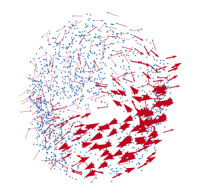
Refer to caption
(a)
Refer to caption
(b)
Refer to caption
(c)
Refer to caption
(d)
Refer to caption
(e)
Refer to caption
(f)
Refer to caption
(g)
Refer to caption
(h)
Refer to caption
(i)
Refer to caption
(j)
Refer to caption
(k)
Figure S5: The first 10 estimated vertex-wise eigenforms on the original dataset 𝐗𝐗{\mathbf{X}} by solving the linear system (S45). Figure LABEL:sub@fig:eth-hhd is the HHD on the first 10 eigenforms, showing that the first two eigenflows are harmonic; the third, fifth, eleventh, thirteenth, and the sixteenth eigenflows are gradient flow, while the rest are curl flows.

The ethanol and malondialdehyde (MDA) datasets [CTS+17] consist of molecular dynamics (MD) trajectories with different amounts of conformational degrees of freedom. A point in the dataset corresponds to a molecular configuration, which is recorded in the xyz format. More specifically, if the molecule has N𝑁N atoms, then a configuration can be specified by a N×3𝑁3N\times 3 matrix. To remove the translational and rotational symmetry in the original configuration space, we preprocess the data by considering two of the angles of every triplet of atoms in a molecule (under the observation that two angles are sufficient to determine a triangle up to a constant). The linear relation is removed by applying Principal component analysis (PCA) with the unexplained variance ratio less than 104superscript10410^{-4}. This generates the original data 𝐗𝐗{\mathbf{X}} with ambient dimension upper bounded by D2(N3)𝐷2binomial𝑁3D\leq 2\cdot\binom{N}{3}. In Figure S5, we estimate the first 10 eigenforms by solving the linear system (S45). The 0-th eigenform clearly represents the bigger loop parameterized by Hydroxyl rotor as shown in the inset scatter plot of Figure 2d. In Figure S5b, it is difficult to tell whether the first eigenflow corresponds to Methyl rotor or not. One can overcome this issue by mapping the first eigenform to the torsion space with prior knowledge as illustrated in Figure 2f. Harmonic flows often represent a global structure; by contrast, flows in Figure S5dS5f are more localized, implying that the eigenflows are not harmonic. The Helmholtz-Hodge decomposition of the eigenvectors of 1subscript1\mathbf{\mathcal{L}}_{1} in Figure S5c confirms this.

Figure S6 shows the scatter plot of the first three principal components of the MDA dataset. As clearly shown in the figures, it is difficult to make sense of the topological structure for the manifold of such dataset is a torus embedded in a 4 dimensional space. With the aid of the first two harmonic eigenforms, one can infer that the first loop travels in the direction of northwest to southeast, while the second loop goes diagonally from northeast to southwest. With proper prior knowledge, one can map the harmonic eigenforms to the torsion space to get a better visualization, as shown in Figure 2i.
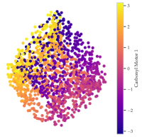
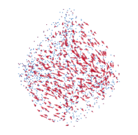
Refer to caption
(a)
Refer to caption
(b)
Refer to caption
(c)
Refer to caption
(d)
Figure S6: The harmonic eigenflows of the MDA dataset. LABEL:sub@fig:mda-eigenform-plots-tau-1 and LABEL:sub@fig:mda-eigenform-plots-tau-2 are the scatter plot of the first three PCs colored by the first and second Carbonyl rotors (purple and yellow in the inset of 2g, see also 2i). LABEL:sub@fig:mda-eigenform-plots-1 and LABEL:sub@fig:mda-eigenform-plots-2 represent the first two harmonic eigenforms estimated from the eigenvectors of 1ssuperscriptsubscript1𝑠\mathbf{\mathcal{L}}_{1}^{s}. The zeroth eigenform in LABEL:sub@fig:mda-eigenform-plots-1 parameterizes the first carbonyl rotor in LABEL:sub@fig:mda-eigenform-plots-tau-1, while the first eigenform in LABEL:sub@fig:mda-eigenform-plots-2 represents the second carbonyl rotor as in LABEL:sub@fig:mda-eigenform-plots-tau-2. See also Figure 2i for a better visualization.

J.3 Ocean drifter dataset

The ocean drifter data, also known as Global Lagrangian Drifter Data, were collected by NOAA’s Atlantic Oceanographic and Meteorological Laboratory. The dataset was used in [FP15] to analyze the Lagrangian coherent structures in the ocean current, showing that certain flow structures stay coherent over time. Each point in the dataset is a buoy at a certain time, with buoy ID, location (in latitude & longitude), date/time, velocity, and water temperature available to the practitioner. We extract the buoys that were in the North Pacific ocean dated between 2010 to 2019. The original sample size is around 333 million, we sampled 1,50015001,500 furthest buoy that meet the above criteria.

The velocity field in the original data depends a lot on the events in the shorter time scale, e.g., wind or faster changing ocean current. In comparison, ocean motions at longer time scale oftentimes are more interesting to the scientists. Therefore, we discard the short-term velocity field in the original data and calculate the the velocity field as follows. We first compute the finite difference of the current location and the next location of the same buoy. The velocity of the buoy at current point is obtained by dividing this quantity by the time difference. The 1-cochain can be constructed by linear approximate of integral as in (S41) after obtaining the velocity field of each point.

J.4 Single cell RNA velocity data

All of the RNA velocity data (Chromaffin, Mouse hippocampus, and human glutamatergic neuron cell differentiation dataset) as well as methods/codes to preprocess them can be found in [LMSZ+18]. The RNA velocity is a point-wise vector field in the ambient space predicting the future evolution of the cell. To generate the 1-cochain, we apply a linear interpolation as in (S41). The number of cells in the Chromaffin, mouse hippocampus, and human glutamatergic neuron cell differentiation datasets are n=384superscript𝑛384n^{\prime}=384, n=18,213superscript𝑛18213n^{\prime}=18,213, and n=1,720superscript𝑛1720n^{\prime}=1,720, respectively. PCA is applied on the RNA expression, resulting in the ambient dimensions of the aforementioned three datasets being D=5𝐷5D=5, 101010, and 222, respectively. We choose the furthest n=800𝑛800n=800 and n=600𝑛600n=600 cells for the mouse hippocampus and the human glutamatergic neuron data when building the simplicial complex. Since the sample size of the Chromaffin dataset is small, we used all the cells in our analysis.
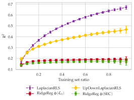
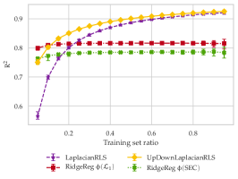
Refer to caption
(a)
Refer to caption
(b)
Refer to caption
(c)
Figure S7: SSL results of the velocity fields of mouse hippocampus cell differentiation dataset with different smoothing parameter k𝑘k.

In the RNA velocity framework, one can control how smooth the generated RNA velocity is by specifying the number of nearest neighbors k𝑘k. The larger this parameter is, the smoother the vector field will become. We show in Figure S7 that the proposed algorithm out-performed other algorithms for several choices of smoothness values. Note that in theory, the UpDownLaplacianRLS should be at least as good as LaplacianRLS algorithm, for the first one is the extension of the second method. However, since we only choose the hyperparameter when train ratio is 0.20.20.2, it is possible that the under-performance of UpDownLaplacian seen in Figure S7a is due to suboptimal choices of parameters.

Appendix K SSL experiments on the divergence free flows
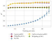
Refer to caption
(a)
Refer to caption
(b)
Refer to caption
(c)
Refer to caption
(d)
Refer to caption
(e)
Refer to caption
(f)
Refer to caption
(g)
Refer to caption
(h)
Refer to caption
(i)
Refer to caption
(j)
Refer to caption
(k)
Refer to caption
(l)
Figure S8: SSL results on various datasets with the 𝐁1subscript𝐁1{\mathbf{B}}_{1}-SSL proposed by [JSSB19]. Columns from left to right correspond to the results of 2D strip, ocean buoy, Chromaffin cell differentiation, and mouse hippocampus cell differentiation dataset. The top row shows the SSL results on the original velocity field with the result of 𝐁1subscript𝐁1{\mathbf{B}}_{1}-SSL (blue curve) added. The second row represents the curl component of the flows in Figure 3 using HHD. The third row are the SSL results of the data with the curl flow shown in the second row.

The 𝐁1subscript𝐁1{\mathbf{B}}_{1}-SSL algorithm proposed by [JSSB19] works on (approximately) divergence-free flow. However, the assumption is not always valid for the flows observed in the many real datasets are often times a mixture of gradient, curl, and harmonic flows. Applying the 𝐁1subscript𝐁1{\mathbf{B}}_{1}-SSL algorithm by [JSSB19] do not results in a good result, as shown in Figures S8aS8d. Note that these figures are identical to Figures 3e3h, but with the SSL results from [JSSB19] (blue curves) added. Except for the synthetic flow, the performances of 𝐁1subscript𝐁1{\mathbf{B}}_{1}-SSL are as bad as random guess.

To further evaluate 𝐁1subscript𝐁1{\mathbf{B}}_{1}-SSL of [JSSB19], in comparison with our 1subscript1\mathbf{\mathcal{L}}_{1} based SSL algorithms, we artificially create data that satisfies the 𝐁1subscript𝐁1{\mathbf{B}}_{1}-SSL assumptions. Namely, we extract the curl component from the computed 1-cochain using HHD. In mathematical terms, we first solve the following linear system to get the vector potential 𝐯^=argmin𝐯n2𝐁2𝐯ω2^𝐯subscriptargmin𝐯superscriptsubscript𝑛2subscriptnormsubscript𝐁2𝐯𝜔2\hat{{\mathbf{v}}}=\operatorname*{argmin}_{{\mathbf{v}}\in\mathbb{R}^{n_{2}}}\|{\mathbf{B}}_{2}{\mathbf{v}}-\mathbf{\omega}\|_{2}. The curl component is obtained by projecting 1-cochain ω𝜔\mathbf{\omega} onto the image of 𝐁2subscript𝐁2{\mathbf{B}}_{2}, i.e., ωcurl=𝐁2𝐯^subscript𝜔curlsubscript𝐁2^𝐯\mathbf{\omega}_{\mathrm{curl}}={\mathbf{B}}_{2}\hat{{\mathbf{v}}}. The estimated velocity field from the curl cochains for each datasets can be found in Figures S8eS8h. As shown in Figure S8iS8l, the proposed algorithms based on both the up and down Laplacian out-perform [JSSB19] for small train/test ratio. In fact, the performance of 𝐁1subscript𝐁1{\mathbf{B}}_{1}-SSL is always weak until the proportion of labeled examples exceeds about 0.70.70.7. For manifolds with simple structure, i.e., 2D plane and ocean dataset, [JSSB19] can achieve almost perfect predictions (R21superscript𝑅21R^{2}\approx 1) when train-test ratio 0.9absent0.9\geq 0.9. However, this is not the case for manifolds with complex structures, e.g., RNA velocity datasets.

Appendix L Choice of regularization parameter λ𝜆\lambda for estimating point-wise velocity field from 1-cochain—vector field from all experiments
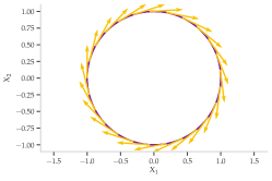
Refer to caption
(a)
Refer to caption
(b)
Refer to caption
(c)
Refer to caption
(d)
Refer to caption
(e)
Refer to caption
(f)
Refer to caption
(g)
Refer to caption
(h)
Refer to caption
(i)
Refer to caption
(j)
Refer to caption
(k)
Refer to caption
(l)
Refer to caption
(m)
Refer to caption
(n)
Refer to caption
(o)
Figure S9: Comparisons of the estimated velocity fields from 1-cochain for various datasets with different regularization coefficient λ𝜆\lambda’s. Columns from left to right are λ=0𝜆0\lambda=0, λρsubscriptsuperscript𝜆𝜌\lambda^{*}_{\rho}, and λMSEsubscriptsuperscript𝜆MSE\lambda^{*}_{\text{MSE}} (see more detail in Supplement I.2 and Figure S3). Rows from top to bottom correspond to the eigenflows of synthetic circle, eigenflows of synthetic torus, eigenflows of synthetic flat torus, eigenflows of ethanol in torsion space, and eigenflows of MDA in torsion space. The last two vector fields are mapped from original PCA space 𝐗𝐗{\mathbf{X}} to torsion space using (S47).
Refer to caption
(a)
Refer to caption
(b)
Refer to caption
(c)
Refer to caption
(d)
Refer to caption
(e)
Refer to caption
(f)
Refer to caption
(g)
Refer to caption
(h)
Refer to caption
(i)
Refer to caption
(j)
Refer to caption
(k)
Refer to caption
(l)
Figure S10: Comparisons of the estimated velocity fields from 1-cochain for various datasets with different regularization coefficient λ𝜆\lambda’s. Columns from left to right are λ=0𝜆0\lambda=0, λρsubscriptsuperscript𝜆𝜌\lambda^{*}_{\rho}, and λMSEsubscriptsuperscript𝜆MSE\lambda^{*}_{\text{MSE}} (see more detail in Supplement I.2 and Figure S3). Rows from top to bottom correspond to the smoothed velocity field of ocean buoy dataset, estimated velocity field from the inverse problem on ocean buoy data, estimated velocity field of the zero-padded cochain on the human glutamatergic neuron data, and the estimated velcoity from the inverse problem on human glutamatergic neuron dataset.