Internal Wasserstein Distance
for Adversarial Attack and Defense
Abstract
Deep neural networks (DNNs) are known to be vulnerable to adversarial attacks that would trigger misclassification of DNNs but may be imperceptible to human perception. Adversarial defense has been an important way to improve the robustness of DNNs. Existing attack methods often construct adversarial examples relying on some metrics like the distance to perturb samples. However, these metrics can be insufficient to conduct adversarial attacks due to their limited perturbations. In this paper, we propose a new internal Wasserstein distance (IWD) to capture the semantic similarity of two samples, and thus it helps to obtain larger perturbations than currently used metrics such as the distance. We then apply the internal Wasserstein distance to perform adversarial attack and defense. In particular, we develop a novel attack method relying on IWD to calculate the similarities between an image and its adversarial examples. In this way, we can generate diverse and semantically similar adversarial examples that are more difficult to defend by existing defense methods. Moreover, we devise a new defense method relying on IWD to learn robust models against unseen adversarial examples. We provide both thorough theoretical and empirical evidence to support our methods.
1 Introduction
Deep neural networks (DNNs) are vulnerable to adversarial examples [1, 2, 3, 4] mainly due to their overfitting nature [5]. Particularly, this issue becomes more severe if we have only limited training data for a specific task. In fact, the neural network tends to fit the training data well and may make an incorrect prediction for an example contaminated by only slight perturbations or transformations. Moreover, the security of deep learning systems is vulnerable to crafted adversarial examples, which may be imperceptible to the human perception but can lead the model to misclassify the output [6, 7]. In practice, adversarial examples can be generated by perturbing or transforming some image pixel values to ensure they maintain the semantic similarity with the original images. Such similarity is a perceptual metric that is often defined by a simple metric such as the distance [8]. However, this metric suffers from two limitations.
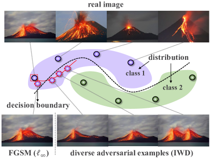
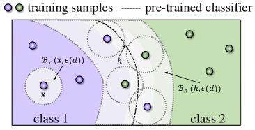
First, most attack methods [8, 9, 3] use the distance as a similarity metric to fool a classifier. However, the metric, despite its computational convenience, is ineffective to elaborate all possible adversarial perturbations (e.g., translation, dilation or deformation) due to its insufficient perturbations. Specifically, the attackers always use this metric to ensure that adversarial examples are bounded in a small norm box to keep the semantic consistency of adversarial examples and original ones, which limits the effectiveness of the adversarial perturbations. As shown in Figure 1, adversarial examples crafted with using FGSM [8] are often close to the original sample, which may result in an ineffective attack when the sample is distant from the decision boundary. Thus, it is difficult for each image to find an effective adversarial example that causes misclassification of the classifier. Therefore, how to measure the similarity of a sample and its adversarial example is very necessary and important.
Second, models trained merely on adversarial examples are vulnerable to the adversarial examples crafted on the manifold with generative models [10, 11]. One possible reason is that those attack methods, used for generating adversarial examples, understand an input image from a one-sided view in Euclidean space and thus may be insufficient to perturb samples on the manifold. In this sense, perturbing a sample on the manifold would be important to achieve a robust model. In this way, we would obtain more diverse and valuable adversarial examples for training. More importantly, diverse adversarial examples can help in covering the blind area of the data distribution to develop robust models [12, 13]. Unfortunately, how to generate diverse adversarial examples and build robust models with them is unknown.
In this paper, we investigate two key questions: 1) how to effectively attack a model on the manifold; and 2) how to build robust models relying on those attacks. Nevertheless, we find the commonly used distance is insufficient when conducting attack and defense to DNNs on the manifold. To address this, we propose an internal Wasserstein distance (IWD). Relying on IWD, we develop a new attack method (called IWDA) to perturb samples on the manifold. Correspondingly, we develop a defense method (called IWDD) to defend against unseen adversarial examples.
The contributions of this paper are summarized as follows:
-
•
We analyze the reasons why the distance is insufficient when doing attacks and defenses. We thus propose an internal Wasserstein distance (IWD) to exploit the internal distribution of data for both attack and defense tasks.
-
•
We propose a novel attack method to craft adversarial examples using the proposed IWD metric. Quantitative and qualitative experiments demonstrate the superiority of the proposed method.
-
•
We theoretically derive an upper bound for the attack classification error, and this motivates us to devise a new defense method relying on IWD, to improve the robustness of the classifier.
2 Related Work
2.1 Adversarial Attack
Attack with the perturbation. DNNs are vulnerable to adversarial examples with a perceptible perturbation [1]. Most existing methods [8, 12, 14, 15, 3] attempt to craft adversarial examples with the perturbation. However, these adversarial examples cannot result in a large perturbation that can guarantee successful attacks. Besides, the perturbation is not a good metric of image similarity [16].
Attack with the non- perturbation. To mitigate the limitations of the perturbations, several methods [16, 17, 15, 18, 19, 20] try to craft adversarial examples beyond the perturbations. To this end, [16] propose an ADef algorithm to craft adversarial examples by deforming images iteratively. In addition, [21] iteratively project adversarial examples onto the Wasserstein ball. To develop stronger and faster attacks, [20] apply projected gradient descent and Frank-Wolfe to craft adversarial examples. However, these adversarial examples may lack diversity. In this paper, we propose a novel metric, internal Wasserstein distance (IWD), to generate diverse adversarial examples.
2.2 Adversarial Defense
To address the vulnerability of DNNs, many defense methods [8, 22] have been proposed to defend against adversarial examples. For example, [9] present a projected gradient descent (PGD) training method to improve the resistance of the model to a wide range of attacks. Unfortunately, training with PGD is time-consuming and computationally intensive [23]. To address this, free-PGD [23] and fast-AT [24] speed up the training and improve the robustness of the model.
Recently, PGD adversarial training is a popular method to defend against adversarial examples. However, most studies [25, 26, 27, 28, 29, 13] posit that a robustness-accuracy trade-off may be inevitable in defense methods. For example, [30] theoretically analyze the trade-off between standard risk and adversarial risk and derive a Pareto-optimal trade-off over some specific classes of models in the infinite data with fixed features dimension. In addition, [31] introduce a Nuclear-Norm regularizer to enforce the function smoothing in the vicinity of data samples to achieve an efficient and effective adversarial training method. Moreover, [32] propose a hybrid Langevin Monte Carlo technique to improve the performance of adversarial training. However, these methods are limited in improving the robustness of a classifier due to the limitations of the distance. In this paper, we derive an upper bound to enhance the robustness relying on the IWD.
3 Notation and Motivations
Notation.
We use calligraphic letters (e.g., ) to denote spaces, and bold lower case letters (e.g., ) to denote vectors. Without loss of generality, we first consider a framework of binary classification, which can be well generalized to the multi-class classification. Let be the real data distribution, and be the training data, where denotes the data and denotes the label. Let be a classifier learned on and valued in . Let be the diameter of a set . Let be an indicator function, where if is true and otherwise. Let be a sufficiently small constant with respect to some metric , and be the -neighborhood set of . Similarly, let be the -neighborhood set of , as shown inFigure 2.
To develop our proposed method, we first provide the definition of the adversarial example as follows.
Definition 1.
(-adversarial example) Given a sample pair , the sample admits an -adversarial example if there exists a sample such that and .
To construct an adversarial example , most existing methods often use the distance as the metric . However, this metric is insufficient when conducting attack and defense.
Limitations of the distance for attack and defense. The distance may only ensure that the crafted adversarial examples are close to the original sample due to small perturbations (seeFigure 1). When performing the attack, if a sample is far away from the decision boundary, it is difficult to find an effective adversarial example that can fool the classifier. Thus, the distance is insufficient to conduct adversarial attacks when a good classifier can well describe the boundaries of different classes with a large margin.
For defense, most existing methods reinforce the training procedure by searching for adversarial examples relying on the distance. In this way, they try to learn a robust classifier to cover the blind area of the data distribution. However, they may fail to cover the whole data distribution due to the limited range of the perturbation, leading to inferior defense performance. To address these, we propose a new metric in this paper to exploit the internal distribution of data for both attack and defense.
3.1 Internal Wasserstein Distance
As aforementioned, the attack and defense methods relying on the distance are insufficient to perturb the samples. Recently, the Wasserstein distance [33] has been proposed to measure the differences between two given distributions and widely used in generated adversarial networks (GANs) [34].
Definition 2.
(1-Wasserstein distance [33]) Given two distributions and of and , respectively, the Wasserstein distance can be defined as:
| (1) |
Here, is a set of all joint distributions whose marginal distributions are and .
Here, we consider -Wasserstein distance following [34]. Concretely, the 1-Wasserstein distance has a well-defined dual formulation and can be developed in WGAN [34] using the Kantorovich-Rubinstein duality [33]. Note that while the Wasserstein distance has been widely used in GANs, it is non-trivial to apply it to conduct adversarial attack, since the Wasserstein distance between two samples in Eqn. (1) is difficult to be defined without defining their distributions. To this end, some methods [21, 20] model it as the moving pixel mass from one whole image to another with EMD distance, which, however, may fail to measure the similarity of images when the internal patch of the image transforms, e.g., swapping the internal patch.
To address this, we propose an internal Wasserstein distance (IWD) to measure the internal distribution distance between a sample and its adversarial sample . Specifically, let and be patches drawn from two samples and , respectively. We define the internal distributions of and as and , respectively, where is the Dirac distribution [35]. Here, we select patches from different scaled images. Specifically, for an image , let be the minimum height of the scaled image and be the minimum size of the patches. Given a scale set with a scale factor , we decompose each scaled image uniformly into patches, where is the sampling rate. Then, we define the IWD as follows.
Definition 3.
(Internal Wasserstein distance) Given internal distributions and of and , respectively, the internal Wasserstein distance can be defined as:
| (2) |
where is a set of all joint distributions whose marginal distributions are and .
Remark 1.
From the definition, IWD is different from the Wasserstein distance. Specifically, the Wasserstein distance in Eqn. (1) is not able to directly calculate the similarity between two samples and without defining their distributions. Although [21] and [20] consider this problem as the moving mass form to , this is not necessarily a good measure of image similarity: e.g., swapping the internal patches of causes their Wasserstein distance if , which will be zero in our IWD, i.e., .
Definition 3 indicates that IWD captures the semantic similarity of two samples with the help of defining distributions of patches in the image, which thus is able to perturb a sample on the manifold when performing attacks. The following theorem indicates that the IWD can lead to larger transformations than the pixel perturbation (e.g., the distance).
Theorem 1.
Let and denote the perturbation constants with the distance and IWD, respectivly. Then for any , there exists satisfies:
Theorem 1 shows that the diameter of the perturbation ball in terms of is larger than that in terms of . Thus, IWD would have a higher probability to find valid adversarial examples that fool the model than the distance. In the following, we apply IWD to perform attack and defense.
4 Adversarial Attack with IWD
In general, the adversarial attack aims to learn an adversarial attacker to confuse a classifier , where can be a random noise vector or other kinds of input. We consider untargeted attack and targeted attack, which can be formulated as the following optimization problems:
| (3) |
where , is the label of and is the label of the targeted attack, is some classification-calibrated loss [36].
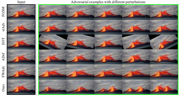
Relying on IWD, we are able to craft semantically similar but diverse adversarial examples. For example, the crafted adversarial examples of a volcano image (see Figure 1) contain one or more volcanoes with different sizes, shapes and locations. However, it is non-trivial to directly apply IWD to perform adversarial attack to obtain such adversarial examples, since the infimum in Eqn.(2) is highly intractable [34]. To conduct adversarial attack with IWD, we next introduce the objective function for attack.
4.1 Objective Function for Attack
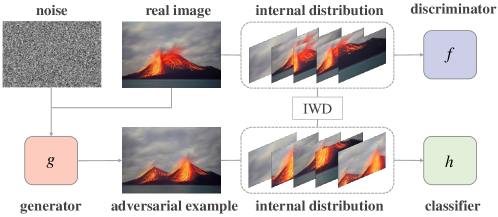
To generate -adversarial examples, we propose a new attack method relying on IWD, called IWDA. Figure 1 (a) illustrates the overall scheme of IWDA. Specifically, we optimize an adversarial attack loss to craft -adversarial examples. Meanwhile, we optimize a classification loss such that the classifier misclassifies the adversarial examples. Then, the total objective function can be written as follows:
| (4) |
where is a hyper-parameter. Next, we introduce the adversarial attack loss and classification loss.
Adversarial attack loss. In Figure 3, the generator aims to produce an adversarial example , and then the discriminator distinguishes the internal distributions of patches in the adversarial example and the original image . Relying on the internal Wasserstein distance, we propose to optimize the following adversarial loss:
| (5) |
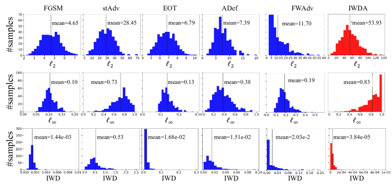
where and denote the internal distributions of patches in and , respectively. Here, is the Lipschitz constant of . In practice, we introduce a gradient penalty [37] to optimize Problem (5). Note that we do not necessarily constrain IWDA adversarial examples bounded in an IWD ball from original images. The IWD distance between adversarial examples and original ones decreases during the training. In Section 6.1, we measure the perturbation distance under the IWD metric. The last sub-figure of Figure 5 shows the distance between IWDA adversarial examples and the original counterparts is close to zero on average under the IWD metric.
Classification loss. The classification loss can be calculated by the distance between the prediction and the ground truth (untargeted attack), or the opposite of the distance between the prediction and the target class (targeted attack). Then, can be written as:
| (6) |
The detailed algorithm is shown in Algorithm 1.
In practice, we select different patches of images by training a pyramid GAN model with different scales progressively in a coarse-to-fine manner. For example, we first set a sliding window (e.g. kernel size = 3) and select patches of the current image , where = imageLength imageWidth / kernelSize2. In this sense, the number of patches in different scales is depended on the image size.
Differences with DeepEMD [38]. The idea of comparing patches of images using the Wasserstein distance can be also referred to other works, e.g., DeepEMD. Concretely, DeepEMD calculates the similarity between local features of two images for few-shot learning. In contrast, IWDA measures the Wasserstein distance of the distribution of patches in two images and aims to craft adversarial examples that can confuse the classifier.
5 Adversarial Defense with IWD
Relying on IWD, our proposed method (IWDA) is able to effectively attack the classifier by distribution perturbations on the manifold. Note that the attack and defense are coupled tasks. Essentially, with sufficient adversarial examples, we are able to learn a robust classifier. In this sense, we propose a new defense method with IWD, called IWDD.
Mathematically, the adversarial defense problem aims to learn a robust classifier to defend against the attacks from an adversarial generator to be learned. Following [9, 23], we can learn and simultaneously by solving the following minimax problem:
| (7) |
However, due to the limitations of the distance, the Solutions like (7) are limited in improving the robustness of a model. By contrast, IWD is able to obtain a large perturbation from Theorem 1. To achieve a robust model, we derive an upper bound to develop our IWDD relying on the IWD.
To begin with, we define the expected classification error as and let . Following [25], we define the attack classification error as below.
Definition 4.
(Attack classification error) Given a sample , if there exists an -adversarial example such that , the attack classification error of a classifier can be defined as:
Based on Definition 4, we derive the following upper bound to achieve the robustness of the model.
Theorem 2.
(Upper bound) Let be the -risk of and its optimum . There exists a concave function on such that and as , we have the following upper bound:
From Theorem 2, we minimize the upper bound such that can be small. In this way, the attack probability can be guaranteed to be sufficiently small. To this end, we propose a robust minimax objective function as follows:
| (8) |
where , and is a hyper-parameter in practice. In Problem (8), the first term aims to minimize the natural classification loss between the prediction and the ground-truth , while the second term encourages generating -adversarial examples. By optimizing Problem (8), the generated adversarial examples can be covered the data distribution to improve the robustness of the classifier.
Extension to multi-class problems. So far, we only focus on the binary classification problem. Actually, for multi-class problems, a surrogate loss is calibrated if minimizers of the surrogate risk are also minimizers of the 0-1 risk [39]. The multi-class calibrated loss also include the cross-entropy loss [25]. Therefore, we generalize Problem (8) to the multi-class classification problems as:
| (9) |
where is the cross-entropy loss. The detailed algorithm is shown in Algorithm 2.
Differences with TRADES [25]. The idea of extending the binary classification to the multi-class classification was also presented in TRADES. However, the perturbation ball they defined in Problem (9) is in the distance and thus they generate adversarial examples by the PGD attack [9]. On the contrary, our IWDD algorithm uses the IWD metric to stimulate diverse adversarial examples to cover the low-density regions of the data, which would lead to better defense performance.
| Model |
|
||||||
|---|---|---|---|---|---|---|---|
| FGSM | stAdv | EOT | ADef | FWAdv | IWDA | ||
| Inception-v3 | 69.78 | 99.45 | 99.73 | 100.00 | 98.34 | 100.00 | |
| Inception-v3 (free-PGD) | 15.51 | 69.31 | 88.12 | 97.36 | 76.24 | 100.00 | |
| Inception-v3 (fast-AT) | 19.17 | 73.31 | 88.72 | 97.74 | 84.21 | 99.34 | |
| ResNet-101 | 89.43 | 99.73 | 99.46 | 100.00 | 100.00 | 100.00 | |
| ResNet-101 (free-PGD) | 18.83 | 61.42 | 91.12 | 97.22 | 74.58 | 100.00 | |
| ResNet-101 (fast-AT) | 17.39 | 60.54 | 94.31 | 97.32 | 74.25 | 99.62 | |
| Inception-v3 (targeted) | 0.27 | 18.96 | 48.63 | 55.77 | - | 90.66 | |
| ResNet-101 (targeted) | 1.90 | 59.35 | 79.13 | 87.26 | - | 94.58 | |
| Model |
|
||||
|---|---|---|---|---|---|
| FGSM | ADef | FWAdv | IWDA | ||
| ResNet-101 (PGD) | 9.53 | 79.77 | 21.39 | 91.55 | |
| ResNet-101 (TRADES) | 7.95 | 75.43 | 26.57 | 92.69 | |
6 Experiments
Dataset. Following [16], We conduct experiments on ImageNet [40]. In addition, we choose 10 classes from ImageNet (called tiny ImageNet), e.g., barn, megalith, alp, cliff, coral reef, lakeside, seashore, valley, volcano, and coral fungus. The results on CIFAR-10 [41] are provided in Supplementary.
Implementation details. We implement our method based on PyTorch and use the architectures of the models following [42]. Specifically, we use two pre-trained classifiers (i.e., Inception-v3 [43] and ResNet-101 [44]) in the attack methods. During the training, we use an Adam optimizer to update the generator and the discriminator models with and and set the learning rate as 0.0005. For the defense, we use an SGD optimizer to train a new classifier with 200 epochs, a learning rate of , and a batch size of 128.
Baselines and evaluation metrics. We compare our attack method with non- and attacks. Specifically, the non- attacks include ADef [16], EOT [15], stAdv [19] and FWAdv [20], while the attack includes FGSM [8]. We use attack success rate (ASR) to measure the probability of successfully attacking the classifier. For defense, we use free-PGD [23], PGD [9], fast-AT [24], TRADES [25] and MART [29] as baselines. We calculate the classification accuracy on clean samples and adversarial examples.
6.1 Experiments on Adversarial Attack
We perform the adversarial attack on Inception-v3 and ResNet-101 models. We use free-PGD [23] and fast-AT [24] to train robust models on ImageNet, while PGD [9] and TRADES [25] on tiny ImageNet. Here, we use free-PGD and fast-AT instead of PGD [9] since PGD is inefficient when training on ImageNet [23]. Note that non- attack methods often lead to deformation, while attack methods move a few pixels in the image. Thus, it is hard to use the same distance metric to measure the similarity between samples when comparing different attack methods ( and non-). Following the settings in [45, 19], we maintain the visual similarity of samples when enforcing attacks.
| Model | Training method | Clean data | PGD-10 | FWAdv |
|---|---|---|---|---|
| Inception-v3 | natural | 83.00 | 0.00 | 0.00 |
| free-PGD | 62.80 | 28.40 | 54.60 | |
| PGD | 70.60 | 45.00 | 53.20 | |
| IWDD | 70.80 | 46.00 | 63.40 | |
| ResNet-101 | natural | 79.80 | 0.00 | 0.00 |
| free-PGD | 41.40 | 24.20 | 36.20 | |
| PGD | 69.20 | 44.00 | 54.40 | |
| fast-AT | 50.80 | 39.40 | 44.60 | |
| TRADES | 70.00 | 45.00 | 51.60 | |
| MART | 62.20 | 44.20 | 51.20 | |
| IWDD | 71.80 | 45.60 | 52.00 |
| 0.001 | 0.01 | 0.1 | 1 | |
| Attack success rate (%) | 92.41 | 94.31 | 100.00 | 100.00 |
| 0.001 | 0.01 | 0.1 | 1 | |
| Accuracy on clean data (%) | 70.20 | 70.00 | 71.00 | 71.40 |
| Accuracy on PGD-10 (%) | 44.60 | 45.20 | 46.00 | 40.00 |
Quantitative comparisons. In Table 1 and Table 2, IWDA achieves the highest ASR than other baselines. It suggests that IWDA is able to generate more effective adversarial examples with the IWD. In contrast, the perturbation based on the by FGSM is insufficient to confuse the classifier. Moreover, EOT, stAdv, ADef and FWAdv based on the non- apply pixel based transformations to improve ASR. However, when attacking a robust model like free-PGD and fast-AT, these methods are difficult to achieve high ASR results since their transformations (e.g., perturbation or distortion) fail to result in a large perturbation in Euclidean space. We provide more attack results in Supplementary.
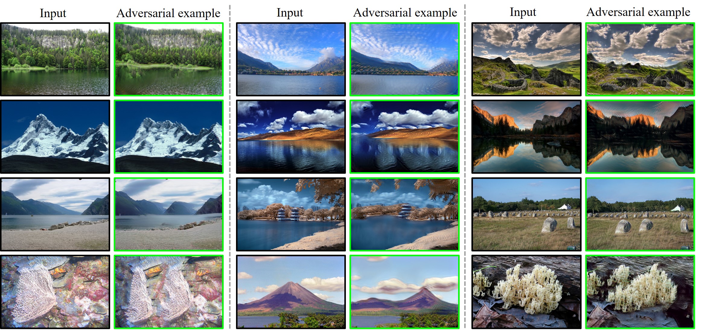
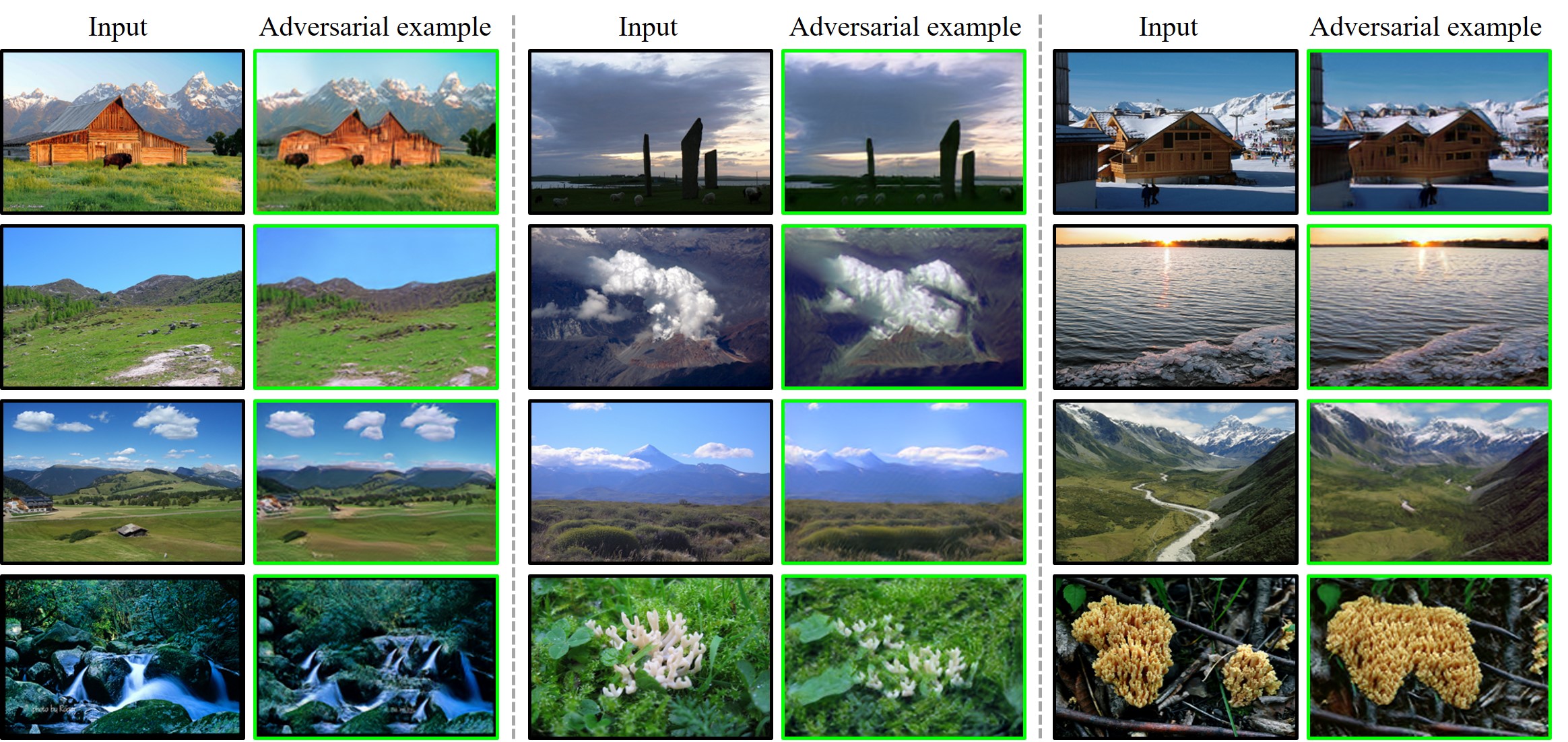
Qualitative comparisons. In Figure 4, our IWDA is able to generate diverse adversarial examples by exploiting the internal distribution of the image. These samples are far away from the input image in Euclidean space and hence cause a large perturbation. Moreover, they are realistic and semantically invariant for human understanding. In this sense, IWDA has good generalization to generate diverse adversarial examples and helps the classifier to understand a real-world image from different views. In contrast, the baselines lack diversity although using a large perturbation to the images. For example, FGSM often destroys the image resolution; EOT keeps the adversarial the same as the original image but changes different rotations; stAdv damages the smoothness of edges of objects; FWAdv reflects shapes and contours in original images but also disrupts the image resolution; ADef maintains the smoothness of the image but deforms the original image. Besides, we show the qualitative results of targeted attack in Supplementary.
Comparisons of perturbation. We further compare the perturbation distance of different methods. Under the untargeted attack setting, we use pre-trained ResNet-101 to generate adversarial examples on tiny ImageNet. Specifically, we measure three metrics (i.e., , and IWD) between a sample and its adversarial example. We count the number of perturbed samples over three metrics. In the first two lines of Figure 5, the adversarial examples using the IWDA achieve the highest mean over the and in Euclidean space compared to baseline methods, thus it has larger perturbations to attack the model. More importantly, in the last line, IWDA achieves the smallest IWD values, even close to zero, suggesting that IWDA is powerful in attacking while keeping the high visual similarity of samples.
6.2 Experiments on Adversarial Defense
We use Inception-v3 and ResNet-101 to demonstrate the robustness of IWDD. We train all defense methods on tiny ImageNet and use PGD-10 [9] and FWAdv [20] to attack the mdoels. We present the clean accuracy and the adversarial accuracy. In Table 3, IWDD achieves a superior or comparable robustness compared to defense baselines. Only against FWAdv on ResNet-101, PGD achieves better performance than IWDD. We believe this is an inherited trade-off between clean accuracy and adversarial accuracy [25]. Other defense baselines like TRADES and MART are limited to improving the generalization on both clean accuracy and adversarial accuracy. Moreover, we put more defense results under AutoAttack [46] in Supplementary.
6.3 Ablation Study
We further evaluate the influences of the hyper-parameters in Eqn. (4) and in Eqn. (9), respectively. By setting different values, we attack the pre-trained ResNet-101 for IWDA and train a robust ResNet-101 for IWDD. The results of attack success rate and validation accuracy are put in Table 4. Empirically, when setting and , IWDA and IWDD achieve superior performance on the trade-off between clean accuracy and robust accuracy.
7 Conclusion
In this paper, we have proposed an internal Wasserstein distance (IWD) to measure the similarity between two samples. Relying on IWD, we propose a novel attack method to generate diverse adversarial examples. Meanwhile, we derive an upper bound and propose a new defense method to improve the robustness of the classifier. Moreover, we analyze the generalization performance of our defense method and prove that robustness requires more diverse adversarial examples in the adversarial training. Extensive experiments on ImageNet confirm the effectiveness of our both attack and defense methods. Furthermore, we expect that a good distance metric will encourage a plethora of researchers to pursue similar tasks in the future.
Acknowledgments
This work was partially supported by Key-Area Research and Development Program of Guangdong Province (2018B010107001, 2019B010155002, 2019B010155001), National Natural Science Foundation of China (NSFC) 61836003 (key project), National Natural Science Foundation of China (NSFC) 62072190, 2017ZT07X183, Tencent AI Lab Rhino-Bird Focused Research Program (No.JR201902), Fundamental Research Funds for the Central Universities D2191240.
References
- [1] Christian Szegedy, Wojciech Zaremba, Ilya Sutskever, Joan Bruna, Dumitru Erhan, Ian Goodfellow, and Rob Fergus. Intriguing properties of neural networks. In International Conference on Learning Representations, 2014.
- [2] Ambar Pal and René Vidal. A game theoretic analysis of additive adversarial attacks and defenses. In Advances in Neural Information Processing Systems, 2020.
- [3] Francesco Croce and Matthias Hein. Mind the box: l1-apgd for sparse adversarial attacks on image classifiers. In International Conference on Machine Learning, 2021.
- [4] Maura Pintor, Fabio Roli, Wieland Brendel, and Battista Biggio. Fast minimum-norm adversarial attacks through adaptive norm constraints. In Advances in Neural Information Processing Systems, 2021.
- [5] Leslie Rice, Eric Wong, and J Zico Kolter. Overfitting in adversarially robust deep learning. arXiv preprint arXiv:2002.11569, 2020.
- [6] Nicolas Papernot, Patrick McDaniel, Ian Goodfellow, Somesh Jha, Z Berkay Celik, and Ananthram Swami. Practical black-box attacks against machine learning. In Proceedings of the 2017 ACM on Asia conference on computer and communications security, pages 506–519, 2017.
- [7] Mahmood Sharif, Sruti Bhagavatula, Lujo Bauer, and Michael K Reiter. Accessorize to a crime: Real and stealthy attacks on state-of-the-art face recognition. In Proceedings of the 2016 acm sigsac conference on computer and communications security, pages 1528–1540, 2016.
- [8] Ian J Goodfellow, Jonathon Shlens, and Christian Szegedy. Explaining and harnessing adversarial examples. In International Conference on Learning Representations, 2014.
- [9] Aleksander Madry, Aleksandar Makelov, Ludwig Schmidt, Dimitris Tsipras, and Adrian Vladu. Towards deep learning models resistant to adversarial attacks. In International Conference on Learning Representations, 2018.
- [10] Yang Song, Rui Shu, Nate Kushman, and Stefano Ermon. Constructing unrestricted adversarial examples with generative models. In Advances in Neural Information Processing Systems, 2018.
- [11] Omid Poursaeed, Tianxing Jiang, Harry Yang, Serge J. Belongie, and Ser-Nam Lim. Fine-grained synthesis of unrestricted adversarial examples. ArXiv, abs/1911.09058, 2019.
- [12] Francesco Croce and Matthias Hein. Reliable evaluation of adversarial robustness with an ensemble of diverse parameter-free attacks. In International Conference on Machine Learning, 2020.
- [13] Divyam Madaan, Jinwoo Shin, and Sung Ju Hwang. Learning to generate noise for multi-attack robustness. In International Conference on Machine Learning, 2021.
- [14] F. Croce and M. Hein. Minimally distorted adversarial examples with a fast adaptive boundary attack. In International Conference on Machine Learning, 2020.
- [15] Anish Athalye, Logan Engstrom, Andrew Ilyas, and Kevin Kwok. Synthesizing robust adversarial examples. In International Conference on Machine Learning, pages 284–293, 2018.
- [16] Rima Alaifari, Giovanni S. Alberti, and Tandri Gauksson. ADef: an iterative algorithm to construct adversarial deformations. In International Conference on Learning Representations, 2019.
- [17] Hsueh-Ti Derek Liu, Michael Tao, Chun-Liang Li, Derek Nowrouzezahrai, and Alec Jacobson. Beyond pixel norm-balls: Parametric adversaries using an analytically differentiable renderer. In International Conference on Learning Representations, 2019.
- [18] Zhengli Zhao, Dheeru Dua, and Sameer Singh. Generating natural adversarial examples. In International Conference on Learning Representations, 2018.
- [19] Chaowei Xiao, Jun-Yan Zhu, Bo Li, Warren He, Mingyan Liu, and Dawn Song. Spatially transformed adversarial examples. In International Conference on Learning Representations, 2018.
- [20] Kaiwen Wu, Allen Houze Wang, and Yaoliang Yu. Stronger and faster wasserstein adversarial attacks. In International Conference on Machine Learning, pages 10377–10387, 2020.
- [21] Eric Wong, Frank Schmidt, and Zico Kolter. Wasserstein adversarial examples via projected sinkhorn iterations. In International Conference on Machine Learning, pages 6808–6817. PMLR, 2019.
- [22] Harini Kannan, Alexey Kurakin, and Ian Goodfellow. Adversarial logit pairing. arXiv preprint arXiv:1803.06373, 2018.
- [23] Ali Shafahi, Mahyar Najibi, Amin Ghiasi, Zheng Xu, John Dickerson, Christoph Studer, Larry S Davis, Gavin Taylor, and Tom Goldstein. Adversarial training for free! In Advances in Neural Information Processing Systems, 2019.
- [24] Eric Wong, Leslie Rice, and J. Zico Kolter. Fast is better than free: Revisiting adversarial training. In International Conference on Learning Representations, 2020.
- [25] Hongyang Zhang, Yaodong Yu, Jiantao Jiao, Eric P Xing, Laurent El Ghaoui, and Michael I Jordan. Theoretically principled trade-off between robustness and accuracy. In International Conference on Machine Learning, 2019.
- [26] Aditi Raghunathan, Sang Michael Xie, Fanny Yang, John C. Duchi, and Percy Liang. Understanding and mitigating the tradeoff between robustness and accuracy. In International Conference on Machine Learning, 2020.
- [27] Yao-Yuan Yang, Cyrus Rashtchian, Hongyang Zhang, Ruslan Salakhutdinov, and Kamalika Chaudhuri. A Closer Look at Accuracy vs. Robustness. In Advances in Neural Information Processing Systems, 2020.
- [28] Jingfeng Zhang, Xilie Xu, Bo Han, Gang Niu, Lizhen Cui, Masashi Sugiyama, and Mohan Kankanhalli. Attacks which do not kill training make adversarial learning stronger. In International Conference on Machine Learning, 2020.
- [29] Yisen Wang, Difan Zou, Jinfeng Yi, James Bailey, Xingjun Ma, and Quanquan Gu. Improving adversarial robustness requires revisiting misclassified examples. In International Conference on Learning Representations, 2020.
- [30] Mohammad Mehrabi, Adel Javanmard, Ryan A. Rossi, Anup B. Rao, and Tung Mai. Fundamental tradeoffs in distributionally adversarial training. In International Conference on Machine Learning, 2021.
- [31] Gaurang Sriramanan, Sravanti Addepalli, Arya Baburaj, and R. Venkatesh Babu. Towards efficient and effective adversarial training. In Advances in Neural Information Processing Systems, 2021.
- [32] Alexander Robey, Luiz F. O. Chamon, George J. Pappas, Hamed Hassani, and Alejandro Ribeiro. Adversarial robustness with semi-infinite constrained learning. In Advances in Neural Information Processing Systems, 2021.
- [33] Cédric Villani. Optimal transport: old and new, volume 338. Springer Science & Business Media, 2008.
- [34] Martin Arjovsky, Soumith Chintala, and Léon Bottou. Wasserstein generative adversarial networks. In International Conference on Machine Learning, pages 214–223, 2017.
- [35] HW Alt. Lineare funktionalanalysis. eine anwendungsorientierte einführung.. aufl. Springer-Verlag, 10:978–3, 2006.
- [36] Peter L Bartlett, Michael I Jordan, and Jon D McAuliffe. Convexity, classification, and risk bounds. Journal of the American Statistical Association, 101(473):138–156, 2006.
- [37] Ishaan Gulrajani, Faruk Ahmed, Martin Arjovsky, Vincent Dumoulin, and Aaron C Courville. Improved training of wasserstein gans. In Advances in Neural Information Processing Systems, pages 5767–5777, 2017.
- [38] Chi Zhang, Yujun Cai, Guosheng Lin, and Chunhua Shen. Deepemd: Few-shot image classification with differentiable earth mover’s distance and structured classifiers. In IEEE/CVF Conference on Computer Vision and Pattern Recognition (CVPR), June 2020.
- [39] Bernardo Ávila Pires and Csaba Szepesvári. Multiclass classification calibration functions. arXiv preprint arXiv:1609.06385, 2016.
- [40] Olga Russakovsky, Jia Deng, Hao Su, Jonathan Krause, Sanjeev Satheesh, Sean Ma, Zhiheng Huang, Andrej Karpathy, Aditya Khosla, Michael Bernstein, Alexander C. Berg, and Li Fei-Fei. ImageNet Large Scale Visual Recognition Challenge. International Journal of Computer Vision, 115(3):211–252, 2015.
- [41] Alex Krizhevsky, Geoffrey Hinton, et al. Learning multiple layers of features from tiny images. 2009.
- [42] Tamar Rott Shaham, Tali Dekel, and Tomer Michaeli. Singan: Learning a generative model from a single natural image. In The IEEE International Conference on Computer Vision, 2019.
- [43] Christian Szegedy, Vincent Vanhoucke, Sergey Ioffe, Jon Shlens, and Zbigniew Wojna. Rethinking the inception architecture for computer vision. In The IEEE Conference on Computer Vision and Pattern Recognition, pages 2818–2826, 2016.
- [44] Kaiming He, Xiangyu Zhang, Shaoqing Ren, and Jian Sun. Deep residual learning for image recognition. In The IEEE Conference on Computer Vision and Pattern Recognition, 2016.
- [45] Logan Engstrom, Brandon Tran, Dimitris Tsipras, Ludwig Schmidt, and Aleksander Madry. Exploring the landscape of spatial robustness. In International Conference on Machine Learning, 2019.
- [46] Francesco Croce and Matthias Hein. Reliable evaluation of adversarial robustness with an ensemble of diverse parameter-free attacks. In ICML, 2020.
- [47] Wei Gao and Zhi-Hua Zhou. On the consistency of multi-label learning. In Proceedings of the annual conference on learning theory, pages 341–358, 2011.
- [48] Tong Zhang. Statistical analysis of some multi-category large margin classification methods. Journal of Machine Learning Research, 5:1225–1251, 2004.
- [49] Chaowei Xiao, Bo Li, Jun-Yan Zhu, Warren He, Mingyan Liu, and Dawn Song. Generating adversarial examples with adversarial networks. In Proceedings of the International Joint Conference on Artificial Intelligence, 2018.
| Supplementary Materials: Learning Defense Transformers for Counterattacking Adversarial Examples |
We organize our Supplementary as follows. In Section A, we prove the Theorem 1 that IWD can result a larger perturbation than the distance. In Section B, we prove the Theorem 2 about the upper bound. In Section C, we give the implementation details for both attack and defense methods. In Section D, we present more experimental results for our proposed methods.
A Proofs of Theorem 1
Proof.
Based on the definition of diameter of a set , i.e.,
we focus on the maximum distance of the set . For convenience of analysis, we use the distance to measure the similarity between any and in the set .
For any to attack methods, the diameter of the satisfies:
| (1) |
where are patches of and , is the dimension of the image . The last inequality follows a fact that the attack, i.e., can lead to the largest perturbation ball in (A) in the attacks. Therefore, we next only compare the attack and IWD attack.
Based on the definition of the internal Wasserstein distance,
where and are internal distributions of and , respectively.
Note that when the patch size of the is scaled down to one, for the case , we have
| (2) |
The result (2) implies attack can be considered as one of the specific cases of the IWD attack.
Next, we discuss the cases that the patch size is grater one. Note that the size of patch is smaller than the orginal image. We can reconstruct the patches of image to craft the adversarial example in the region of . Without loss of generality, we partition an image into two equal parts, i.e., , and assume that . Then, we suppose the adversarial example is disrupted the order of these two block, i.e., . Relying on the definition of the internal Wassersein distance, we have
However, the distance between and satisfies that
| (3) |
Combine formulas A and A to achieve
| (4) |
∎
B Proofs of Theorem 2
To develop our theoretical analysis, we first give the definition of classification boundary term and give the following lemma.
Lemma 1.
Let the classification boundary term be defined as and the expected classification error as . The robust classification error can be decomposed into
| (5) |
Proof.
When being far away from the classification boundary, if the sample is classified correctly (i.e., ), its perturbation is also correct (i.e., ). On the other hand, if the sample is misclassified (i.e., ), then its adversarial example is also misclassified (i.e., ), then . When within the classification boundary, the sample is classified correctly, while its perturbation is misclassified, then . Moreover, the difference between these two terms is . ∎
Based on the definition of classification boundary term, we derive the following lemma to develop Theorem 2.
Lemma 2.
Let be the -risk of a function and its optimum . There exists a concave function on such that and as , we have
| (6) |
Proof.
For the binary classification, the prediction is a vector function, and each element of is in . According to [47], the surrogate loss can be defined as
where is a convex function, is the number of labels, is the -th element of and is the -th element of . For example, the hinge loss , exponential loss , least squares loss and logistic regression loss . Based on Lemma 1, we have
The second line follows by Corollary 26 of [48], it guarantees there exists a concave function on such that and as and
∎
Theorem 2 (Upper bound) Let be the -risk of a function and its optimum . There exists a concave function on such that and as , we have
| (7) |
Proof.
Relying on the conditions of Theorem 2, we have the following upper bound,
where the first two lines follows by Theorem 2. The third line is based on the definition of and . The fourth line follows by a fact that contains more perturbed samples than .
The fifth line satisfies because and are valued in . The last two lines hold by the definition of the surrogate loss [47], i.e.,
This loss includes the hinge loss , exponential loss , least squares loss and logistic regression loss , etc. These losses have a property that
Therefore, we have
∎
C More Implementation Details
C.1 Details of Attack
In our implementation, We use a natural training method, a free-PGD and fast-AT training methods to train the classifiers (Inception-v3 and ResNet-101) on ImageNet. The test accuracies on tiny ImageNet are in Table A. In the following, we introduce the detailed settings for the attack.
Untargeted attack. we train the GAN model with different scaled images to generate adversarial examples. Specifically, we set the scale factor , the minimum height and the minimum size of the patches . For each scale, we train each GAN model 2000 times. To perform IWDA, we first use a set of noise vectors and an original image as inputs of the generator , and use the original image as the input of the discriminator . To achieve better performance, we use a PGD-10 adversarial example as the input of the discriminator. Then, we introduce a classifier at the last scale of updating the GAN model. Actually, we are able to attack the classifier at any scale.
In the optimization, we maximize the cross entropy loss with to generate adversarial examples. At each iteration, we update the generator and discriminator with a step of 3. We use an Adam optimizer to optimize the parameters of the GAN model. We decay the learning rate of optimizer with a milestones of 1600 and a gamma of 0.1 at each training process. Other experiments setup are the same as the untargeted attack.
| Classifier | Inception-v3 | Inception-v3 (free-PGD) | Inception-v3 (fast-AT) | ResNet-101 | ResNet-101 (free-PGD) | ResNet-101 (fast-AT) |
|---|---|---|---|---|---|---|
| Accuracy (%) | 72.80 | 60.60 | 59.80 | 73.80 | 64.80 | 53.20 |
Targeted attack. We further conduct targeted attack experiments with random target labels. In contrast to the untargeted attack setting, we perform the targeted attack at each scale. In the optimization, we minimize the cross entropy loss with . First, we train each GAN model with 2000 iterations. At each iteration, we update generators and discriminators with 3 steps. Then, we update the generators with the cross entropy loss only at the first step. We use the same optimizer settings as the untargeted attack.
Detailed settings for attack methods. We conduct experiments of adversarial attack with the following parameter settings. For FGSM [8], we let be the magnitude of the perturbation; for stAdv [19], we set ; for EOT [15], we set the rotation range at ; for ADef [16], we set , overshot and iterations ; for FWAdv [20], we use the PGD Dual Proj algorithm and set to obtain the worst attack.
C.2 Details of Defense
Training of the GAN model. For the proposed defense method, we use our attack method by updating the generators and discriminators to generate more realistic and diverse adversarial examples. However, the training cost is very expensive. To address this, we pre-train the GAN model to prepare more diverse adversarial examples for adversarial training. Meanwhile, we train a universal generator to generate adversarial examples for efficiency. Following the settings of [49], we pre-process the size of input images as 224 224. Then, we use an Adam optimizer to train the GAN models with 200 epochs, a learning rate of 0.001, and to optimize the parameters of GAN models. Moreover, we decay the learning rate of optimizer with per 50 epochs. We conduct this experiment on two NVIDIA Titan Xp GPUs.
Training of the classifier. We further conduct adversarial training experiments to train the classifiers (i.e., Inception-v3 and ResNet-101). First, we pre-process all input images as for Inception-v3 and for ResNet-101, respectively. Following [16], we perturb the input images of the generator using the PGD algorithm before each iteration of the training process. To optimize Loss (8), we set . Specifically, we train the classifier with 200 epochs. We use an SGD optimizer with a learning rate of 0.1, a momentum of 0.9 and a weight decay of 0.0005, and we decay the learning rate of optimizer with at epoch and epoch , respectively. We conduct this experiment on four NVIDIA Titan Xp GPUs.
Testing of the defense method. We finally test our robust model and other adversarial training models on both clean data and adversarial examples generated by PGD and FWAdv, as shown in Table 3. Following [9], we use the step size of and the clip epsilon of to generate the adversarial examples in PGD attack. For FWAdv attack, we use the PGD Dual Proj algorithm and set to obtain the adversarial examples following [20].
D More Experimental Results
D.1 More Quatitative Results of IWDA
Comparisons with attack methods on CIFAR-10. We also compare our IWDA with other attack methods under the untargeted attack on CIFAR-10 over ResNet18 and demonstrate the attack success rate (ASR) in Table B. IWDA achieves the higher ASR than other baseline methods, which is consistent with the results on ImageNet in Table 1.
| Model | FGSM | stAdv | EOT | ADef | FWAdv | IWDA |
|---|---|---|---|---|---|---|
| Resnet-18 | 54.18 | 95.83 | 85.13 | 99.16 | 97.33 | 99.89 |
| Resnet-18(PGD) | 37.89 | 41.53 | 54.38 | 97.44 | 38.19 | 98.42 |
Robustness of IWDD against IWDA. We use IWDA method to attack the IWDD model and provide the classification accuracy of the IWDD model. From Table C, the IWDD model achieves 5.40% and 6.00% classification accuracy for ResNet-101 and Inception-v3, respectively. We believe training a universal generator to craft adversarial examples for training in IWDD is efficient and effective to defend against attacks such as PGD and FWAdv in Table 3, while it is still difficult to defend against the adversarial examples crafted with IWDA. This phenomenon stems from the power of IWDA elaborately crafting adversarial examples to each sample with a tailored generative model. We postulate that the key to addressing this robustness is training a universal generator that is able to generate tailored adversarial examples for each sample with some conditional information, e.g., the label embedding. We hope that future research will investigate this robustness problem.
| Model | PGD-10 | IWDA | |
|---|---|---|---|
| ResNet-101 | PGD | 44.00 | 5.00 |
| IWDD | 45.60 | 5.40 | |
| Inception-v3 | PGD | 45.00 | 5.60 |
| IWDD | 46.00 | 6.00 | |
D.2 More Qualitative Results of IWDA
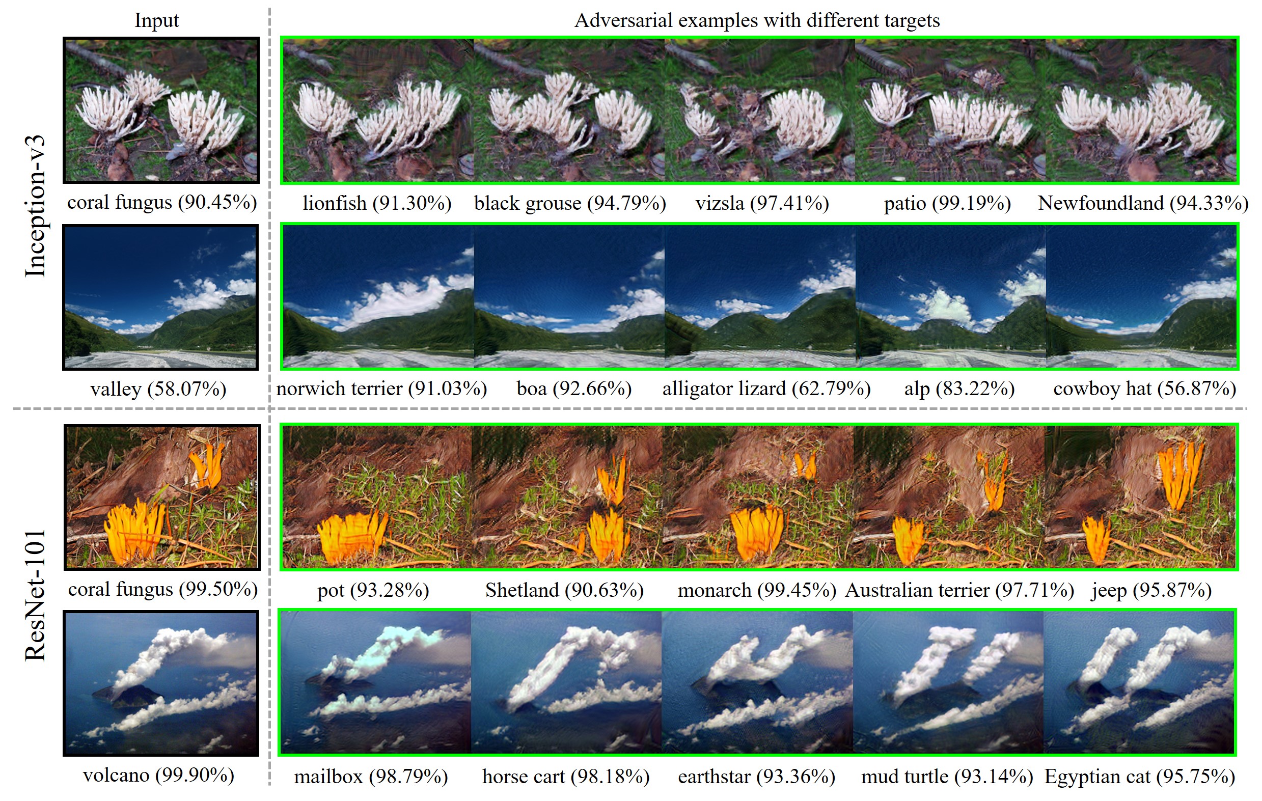
We perform our untargeted attack with the pre-trained Inception-v3 and ResNet-10 on ImageNet and present more qualitative results in Figure A and Figure B, respectively. Moreover, we perform the targeted attack in Fig C. These results suggest that our IWDA has good generalization performance to generate diverse and real adversarial examples and helps the classifier to understand a real-world image from different views.
D.3 More Quatitative Results of IWDD
To further evaluate the robustness of our IWDD, we compare with other baselines under AutoAttack [46]. In Table D, IWDD achieves superior or comparable robustness.
| Defense | Clean data | APGDCE | APGDT | FABT | Square | AA |
|---|---|---|---|---|---|---|
| PGD | 69.20 | 42.60 | 40.80 | 42.00 | 50.40 | 40.80 |
| TRADES | 70.00 | 44.00 | 41.60 | 45.00 | 47.60 | 41.60 |
| MART | 62.20 | 43.60 | 40.20 | 41.40 | 45.60 | 40.20 |
| IWDD | 71.80 | 44.40 | 43.40 | 44.60 | 50.40 | 43.20 |
