Understanding Invariance via Feedforward Inversion
of Discriminatively Trained Classifiers

Supplementary Material
Understanding Invariance via Feedforward Inversion
of Discriminatively Trained Classifiers

Abstract

A discriminatively trained neural net classifier can fit the training data perfectly if all information about its input other than class membership has been discarded prior to the output layer. Surprisingly, past research has discovered that some extraneous visual detail remains in the logit vector. This finding is based on inversion techniques that map deep embeddings back to images. We explore this phenomenon further using a novel synthesis of methods, yielding a feedforward inversion model that produces remarkably high fidelity reconstructions, qualitatively superior to those of past efforts. When applied to an adversarially robust classifier model, the reconstructions contain sufficient local detail and global structure that they might be confused with the original image in a quick glance, and the object category can clearly be gleaned from the reconstruction. Our approach is based on BigGAN (Brock, 2019), with conditioning on logits instead of one-hot class labels. We use our reconstruction model as a tool for exploring the nature of representations, including: the influence of model architecture and training objectives (specifically robust losses), the forms of invariance that networks achieve, representational differences between correctly and incorrectly classified images, and the effects of manipulating logits and images. We believe that our method can inspire future investigations into the nature of information flow in a neural net and can provide diagnostics for improving discriminative models. We provide pre-trained models and visualizations at https://sites.google.com/view/understanding-invariance/home.

1 Introduction

Discriminatively trained deep convolutional networks have been enormously successful at classifying natural images. During training, success is quantified by selecting the correct class label with maximum confidence. To the extent that training succeeds by this criterion, the output must be invariant to visual details of the class instance such as brightness changes, object pose, background configurations or small amounts of additive noise. Consequently, the net is encouraged to discard information about the image other than the class label. A dog is a dog whether the input image contains a closeup of a black puppy in a field or an elegant white poodle being walked on a city street.

The successive layers of a convolutional net detect increasingly abstract features with decreasing spatial specificity, from pixels to edges to regions to local object components—like eyes and legs—to objects—like dogs and cats (Zeiler and Fergus,, 2014). Is is commonly believed that this sequence of transformations filters out irrelevant visual detail in favor of information critical to discriminating among classes. This view is generally supported by methods that have been developed to invert internal representations and recover the visual information that is retained by the representation in a given layer (Mahendran and Vedaldi,, 2015; Dosovitskiy and Brox, 2016a, ; Dosovitskiy and Brox, 2016b, ; Zhang et al.,, 2016; Shocher et al.,, 2020). Inversion of layers close to the input yield accurate reconstructions, whereas inversion of deep layers typically results in a loss of visual detail and coherence. Attempts to determine what visual information remains in the class output distribution, as expressed by the logits that are passed into the final softmax layer, have not been particularly compelling. A notable attempt to invert the logits is the work of Dosovitskiy and Brox, 2016a , which recovered colors, textures and the coarse arrangement of image elements from the logits. However, the reconstructions appear distorted and unnatural, and in the eleven examples shown in Dosovitskiy and Brox, 2016a (, Figure 5), only about half of the object classes are identifiable to a human observer. One would not confuse the reconstructions with natural images. Although many visual details are present, the essence of the objects in the original image is often absent.

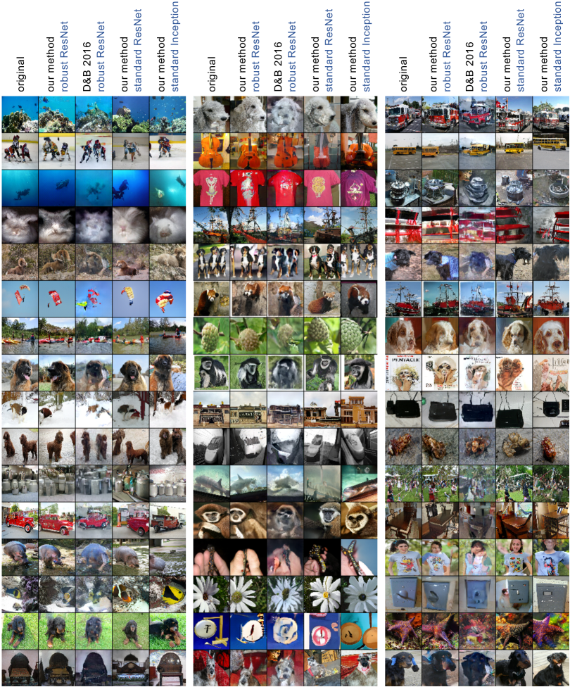
In this paper, we demonstrate that the logit vector of a discriminatively trained network contains surprisingly rich information about not only the visual details of a specific input image, but also the objects and their composition in a scene. With a method that leverages a combination of previously proposed techniques (Dosovitskiy and Brox, 2016a, ; Brock et al.,, 2018), we obtain remarkably high fidelity reconstructions of a source image from the logit vector of an ImageNet classifier. To give the reader a peek ahead, examine Figure 1 and compare the original image in column 1 of each set of five similar images to our reconstruction in column 2. We show that the failure of previous efforts was not due to the loss of instance-specific visual information in the logits, but due to the less powerful inversion machinery. Apart from offering high quality reconstructions, our approach is computationally efficient and flexible for studying the reconstructions under various manipulations on the logits. We therefore leverage our method to explore the properties of logit representations across architectures and optimization methodologies; we particularly focus on comparing the properties of robust logits, optimized with an adversarial training loop (Goodfellow et al.,, 2015), and standard logits, trained with a standard (non-robust) optimizer. Our contributions are as follows:

Figure 1: Original images and logit reconstructions. In each set of five images, the columns are: (1) the original image input to the classifiers, (2) reconstruction from our method using logits of a robust ResNet-152, (3) reconstruction from the method of Dosovitskiy and Brox, 2016a using logits of a robust ResNet-152, (4) reconstruction from our method using logits of a standard (non-robust) ResNet-152, and (5) reconstruction from our method using logits of a standard (non-robust) Inception-V3. The images are selected at random from the test set with the only constraint that all classifiers produced the correct response to the images. These images were not used for training either the classifier or the reconstruction method.

• We improve on existing feature inversion techniques by leveraging conditional projection discriminators and conditional batch-norm. Compared to prior work Dosovitskiy and Brox, 2016a ; Dosovitskiy and Brox, 2016b , this method generates higher qualitative reconstructions and is simpler to implement.

• We show that both classifier architecture and optimization procedure impact the information preserved in logits of a discriminatively trained model. In particular, robust classifiers show significantly better reconstructions, suggesting that robust logits encode more object- and shape-relevant detail than non-robust logits. Further, a ResNet architecture appears to preserve more geometric detail than an Inception architecture does.

• We leverage our inversion technique to explore logit reconstructions for: (1) correctly classified images (and transforms that yield the same response) (2) incorrectly classified images, (3) adversarially attacked images, (4) manipulations in logit space, including shifts, scales, perturbations, and interpolations, and (5) out-of-distribution data.

• Our experiments show that robust logits behave differently than non-robust logits. Most notably, our inversion model of robust logits, trained on ImageNet, can invert data from other datasets without retraining. This supports the view that adversarial training should be used in real-life scenarios when out of domain generalization is important.

2 Related research

Methods developed to invert representations in classification networks fall into two categories: optimization based and learning based. Optimization based methods perform gradient descent in the image space to determine images that yield internal representations similar to the representation being inverted, thus identifying an equivalence class of images insofar as the network is concerned. Back propagation through the classification network is used to compute gradients in input space. For example, Mahendran and Vedaldi, (2015) search over image space, $x\in\mathbb{R}^{H\times W\times C}$, to minimize a loss of the form:

$$\mathcal{L}(x,x_{0})=||\Phi(x)-\Phi(x_{0})||_{2}+\lambda\mathcal{R}(x),$$ (1)

where $x_{0}$ is the original image, $\Phi(x)$ is the deep feature representation of input $x$, $\mathcal{R}$ is a natural image prior, and $\lambda$ is a weighting coefficient. One drawback of this method is that the solution obtained strongly depends on the random initialization of the optimization procedure. With $\lambda=0$, the inverted representation does not resemble a natural image. Engstrom et al., (2019) argued that training a model for adversarial robustness (Madry et al.,, 2017) provides a useful prior to learn meaningful high-level visual representations. To make their argument, they reconstruct images from representation vectors from the penultimate layer of a robust model using the iterative method. They showed reconstructions for a few examples and found that the recovered image is less sensitive to the initial state of the gradient-based search, and that image-space gradients are perceptually meaningful.

Learning based methods use a separate training set of {logits, image pixels} pairs to learn a decoder network that maps a logit vector to an image (Dosovitskiy and Brox, 2016a, ; Dosovitskiy and Brox, 2016b, ; Nash et al.,, 2019; Rombach et al.,, 2020). After training, image reconstruction is obtained via feedforward computation without expensive iterative optimization. For example, Dosovitskiy and Brox, 2016b train a decoder network via a pixel reconstruction loss and an image prior. To improve the blurry reconstructions, Dosovitskiy and Brox, 2016a followed up with an approach most similar to ours, in which they add an adversarial loss to the reconstruction and perceptual losses, which substantially improves the reconstruction quality. We follow a similar approach, but make use of recent advances in generative modelling such as conditional projection discriminators and conditional batch normalization. These modification give higher quality results, and result in a model that is less sensitive to hyperparameter tuning.

3 Models

Figure 2: A pretrained and fixed-weight classifier provides logit vectors which are used by a conditional GAN (Mirza and Osindero,, 2014) to generate reconstructions. The discriminator is based on the projection discriminator of (Miyato and Koyama,, 2018), which is fooled when both the reconstructed image looks natural and is a match to the logit vector of the real image, $x$.

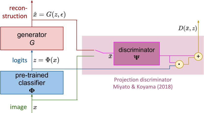
We adopt a learning based approach for reconstructing from the logits. Specifically, we train conditional GANs (Mirza and Osindero,, 2014) to synthesize images. Given an original image $x$ that is passed through a pre-trained classifier $\Phi$ to obtain an $n_{c}$-dimensional logit vector, $z=\Phi(x)$, our method focuses on obtaining a reconstruction of the input, $\hat{x}$, from a generative model $G$ that is conditioned on $z$: $\hat{x}=G(z,\epsilon)$, where $\epsilon\sim\mathcal{N}(0,1)$ is a 120-dimensional noise vector that is used to obtain diversity in the generator output.

We build on the work of Dosovitskiy and Brox, 2016a by using state-of-the-art classifiers and a powerful, elegant adversarial model. Specifically, we leverage batch-norm generator conditioning—first used for style transfer (Dumoulin et al.,, 2016; De Vries et al.,, 2017), and later used in GANs (Miyato and Koyama,, 2018; Brock et al.,, 2018); and projection discriminators—first introduced in Miyato and Koyama, (2018) and further popularized by BigGAN (Brock et al.,, 2018). Instead of conditioning the model components using a one-hot class representation, we condition on the target logit distribution, $\Phi(x_{0})$. Such feature-based conditioning of the discriminator is similar to Boundless (Teterwak et al.,, 2019), and the feature conditioning of the generator is similar to SPADE (Park et al.,, 2019), also known as GauGan.

The generator network is trained to synthesize images that can fool a discriminator network. The weights of both networks are optimized jointly. The discriminator, $D(\bar{x},z)$, takes either a real image, $\bar{x}\equiv x$, or its corresponding generated image, $\bar{x}\equiv\hat{x}$, along with the logit vector $z$ which is either produced by the classifier for the real image, or is used to synthesize the generated image. The discriminator outputs a scalar, a large positive value when $\bar{x}$ is real and a large negative value when $\bar{x}$ is synthetic.

The discriminator consists of two terms, one of which makes the judgment based on whether the image is naturalistic and the other based on whether the image would have produced the given logits. Inspired by the projection discriminator of Miyato and Koyama, (2018), we use

$$D(\bar{x},z)=\left(w_{1}+W_{2}z\right)^{\top}\Psi(\bar{x}),$$ (2)

where $\Psi(\cdot)$ is a deep net that maps to a $n_{d}$-dimensional feature vector; and $w_{1}\in\mathbb{R}^{n_{d}}$, $W_{2}\in\mathbb{R}^{n_{d}\times n_{c}}$. The $w_{1}$ term helps discriminate images based on whether they appear real or synthetic, and the $W_{2}$ term helps to discriminate images based on whether or not they are consistent with the logit vector $z$. The overall architecture is shown in Figure 2.

For an image $x$ and its corresponding logit vector $z=\Phi(x)$, we have adversarial losses for the discriminator $D$, and the generator $G$:

$$\mathcal{L}_{D} =\mathbb{E}_{x,\epsilon}\left[\max\left(-1,D\left(\bar{G}(z,\epsilon),z\right)\right)-\min\left(1,D(x,z)\right)\right],$$

$$\mathcal{L}_{G} =-\mathbb{E}_{x,\epsilon}\left[\bar{D}(G(z,\epsilon),z)\right],$$

with $z=\Phi(x)$, generator noise distribution $\epsilon\sim\mathcal{N}(0,1)$, and $\bar{G}$ and $\bar{D}$ denoting the parameter-frozen generator and discriminator, respectively.

The discriminator is optimized to distinguish real and synthetic images based both on the images themselves and the logit vector. As a result, the discriminator is driven to distill the classification network and then apply a form of adversarial perceptual loss (Johnson et al.,, 2016). The generator is optimized to fool the discriminator by synthesizing images that are naturalistic and consistent with the given logit vector. Consequently, the discriminator must implicitly learn the mapping performed by the classifier $\Phi(x)$.

Dosovitskiy and Brox, 2016a were able to approximately invert representations by using a loss with three terms—adversarial, perceptual, and pixel reconstruction—which requires hyperparameter tuning. The approach we present has the advantage of using a single loss term and thereby avoiding tuning of relative loss weights.

Most of the previous conditional GANs uses the one-hot class label vector for conditioning the generators (Brock et al.,, 2018). Our generator $G$ conditions on the logic vector $z$ instead. Following Brock et al., (2018), we do not treat the conditioning vector $z$ as a conventional input layer for $G$, but rather use $z$ to modulate the operation of each batch-norm layer for a given channel $k$ and a given layer $l$ in $G$ as follows:

$$y^{\prime}_{lk}=\frac{y_{lk}-\mathbb{E}[y_{lk}]}{\mathbb{S}[y_{lk}]}\gamma_{lk}(z)+\beta_{lk}(z)$$ (3)

where $y$ and $y^{\prime}$ are the layer input and output; $\gamma(.)$ and $\beta(.)$ are differentiable functions of $z$, which we implement as two-layer MLPs; and the expectation $\mathbb{E}$ and standard deviation $\mathbb{S}$ are computed over all units in channel $k$ over all inputs in the batch of examples being processed.

4 Methods

We explore three pretrained ImageNet models: ResNet-152-V2 (He et al.,, 2016), Robust ResNet-152-V2 (Qin et al.,, 2019), and Inception-V3 (Szegedy et al.,, 2016). The implementations we used are linked under the model names.

We train generators to produce $64\times 64$ images, and therefore use $64\times 64$ images for input. We modify the BigGAN implementation in the compare_gan code base to support our new conditioning, with the configuration as described in the Supplementary Materials. We train the generator on TPUv3 accelerators using the same ImageNet (Russakovsky et al.,, 2015) training set that the classifiers are trained on, and evaluate using the test set.

We also replicated the method of Dosovitskiy and Brox, 2016a , upgrading the AlexNet classifier they were inverting to a state-of-the-art model. We were able to retrain their method, using their official Caffe (Jia et al.,, 2014) implementation, to invert the logits from the robust ResNet-152.

5 Results

5.1 Comparing reconstruction methods

We begin by comparing reconstructions from our method with those from the method of Dosovitskiy and Brox, 2016a . These reconstructions are shown in columns 2 and 3 of the image sets in Figure 1, respectively, and can be compared to the original images in column 1. Both methods are trained using robust ResNet-152 logits. The images shown in the Figure were not used for training, either the classifier or the reconstruction method. Although both methods capture color and texture well, and both methods seem to generate sensible reconstructions in a quick glance for scenes that are basically textures—such as the underwater seascapes—the Dosovitskiy and Brox, 2016a method fails in recovering object shape, details, and the relationships among parts. For example, distinguishing one dog species from another is quite challenging, and the rabbit is a fuzzy blur.

5.2 Reconstruction from different classifiers

We now turn to exploring reconstructions using our method, trained for different classifiers. In particular we direct the reader to columns 2, 4, and 5 of each image set, which correspond to reconstructions using a robustly trained ResNet-152 (Qin et al.,, 2019), a standard ResNet-152 (He et al.,, 2016), and a standard Inception-V3 (Szegedy et al.,, 2016). Between columns 2 and 4 we can compare adversarial robust training to standard training with the same architecture, and between columns 4 and 5 we can compare different architectures under the same (standard) training procedure.

Before examining these detailed differences, we note that overall the reconstructions from all models capture significant detail about the visual appearance of the image, more than just its class label. In a quick glance, the reconstruction would convey very similar information as the original image. In general, color, texture details, and backgrounds are preserved. However, other information is not preserved, including: left-right (mirror) orientation, precise positions of the image elements, details of the background image context, and the exact number of instances of a class (e.g., the hockey players or the black, white, and brown dogs). The loss of left-right reflection and image-element positions may be due to the fact that these classifier models are trained with the corresponding data augmentations. From those reconstructions we conclude that the logit vector of a discriminatively trained classifier network indeed contains rich information about the input images that could be extracted to reconstruct the input with high fidelity in visual details.

Engstrom et al., (2019) showed that optimization-based feature inversion is significantly improved when using robustly trained classifier models. The reason could be either that the input-space gradients are more perceptually relevant, or that the robust features actually encode more information, or both. Being a learning-based method, our model is not dependent on the input-space gradients. As a result, when we invert robust logits, we can answer the question whether adversarial optimization encodes more instance level information than standard optimization. Examining Figure 1, the robust model reconstructions (column 2 of the image sets) match the original image (column 1) better than the corresponding non-robust model reconstructions (column 4), capturing both local and global detail of the images. For example, the fourth-from-bottom row of the middle collection of images shows a small animal on human skin more clearly; and the cello in the second row is more discernible in the robust model than in the non-robust model. Therefore our results are fully in agreement with prior work such as Engstrom et al., (2019) and Santurkar et al., (2019): robust models are indeed superior to non-robust models in terms of information captured in the logit layer.

Comparing the two non-robust models, ResNet-152 (column 4) and Inception V3 (column 5), the reconstructions from ResNet seem to be truer to the original image, but the reconstructions from Inception are often closer to photorealism. For example, in the middle collection of images, the red t-shirt is reconstructed as purple with a very different design. And in the first row, middle collection, the ResNet dog better matches the original than the Inception dog. The Inception images are more stereotypical. Interestingly, ResNet-152 achieve much better classification performance than Inception. It is a bit surprising that a model that better at classification actually retains richer information relevant to per-instance visual details in the logit vectors.

These findings are further supported by a small-scale human evaluation (4 subjects). Each subject was asked to perform three two-alternative forced choice tasks, each task with 64 images. In each task, the subjects compared pairs of reconstructed images to a ground truth image and were asked to indicate which of the reconstructions was closer to ground truth. As the results in Table 1 indicate: (1) reconstructions by our method is overwhelmingly preferred to that of Dosovitskiy and Brox, 2016a for the same architecture; (2) a robust ResNet is overwhelmingly preferred to a non-robust ResNet with the same loss; and (3) among non-robust networks, ResNet is slightly preferred over Inception.

For each of the four networks, we also computed the LPIPS metric (Zhang et al.,, 2018) over a set of images (Table 2). We see that the metric generally supports the preferences of Table 1 except for the comparison between our method and that of Dosovitskiy and Brox, 2016a , which slightly favors the latter. We believe the reason for this discrepancy is that Dosovitskiy and Brox, 2016a train by minimizing a perceptual loss very similar to that of LPIPS. This highlights the bigger challenge of creating metrics that are not also used as optimization criteria.

Our Robust ResNet vs. D&B Robust ResNet

Ours: 87.5%; D&B: 12.5%

Our Robust ResNet vs. Our Non-Robust ResNet

Robust: 76.5%; Non-robust: 23.5%

Our ResNet vs. Our Inception

ResNet: 52.7%; Inception: 47.3%

Table 1: Two-Alternative Forced Choice (4 subjects, 64 images): “Which reconstruction is closer to the ground truth?"

Robust Ours	0.3138
Robust D+B	0.3092
Non-robust resnet	0.3755
Inception-V3	0.3881

Table 2: LPIPS Between Input and Reconstruction (lower is better)

5.3 Visualizing Model Invariances

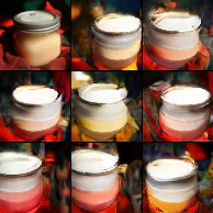
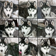
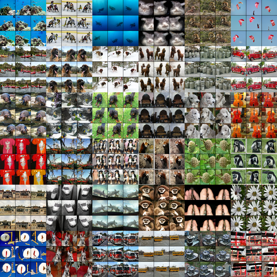
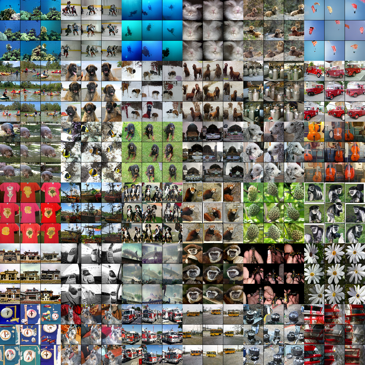
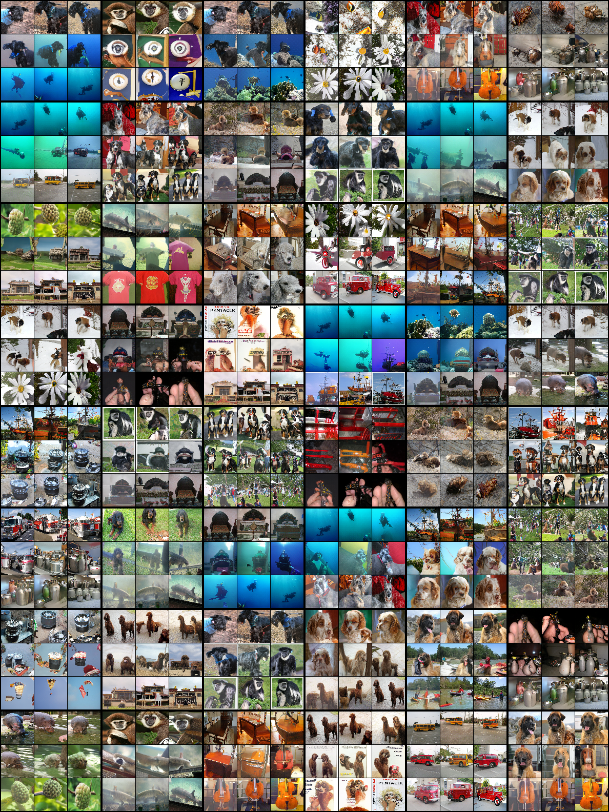
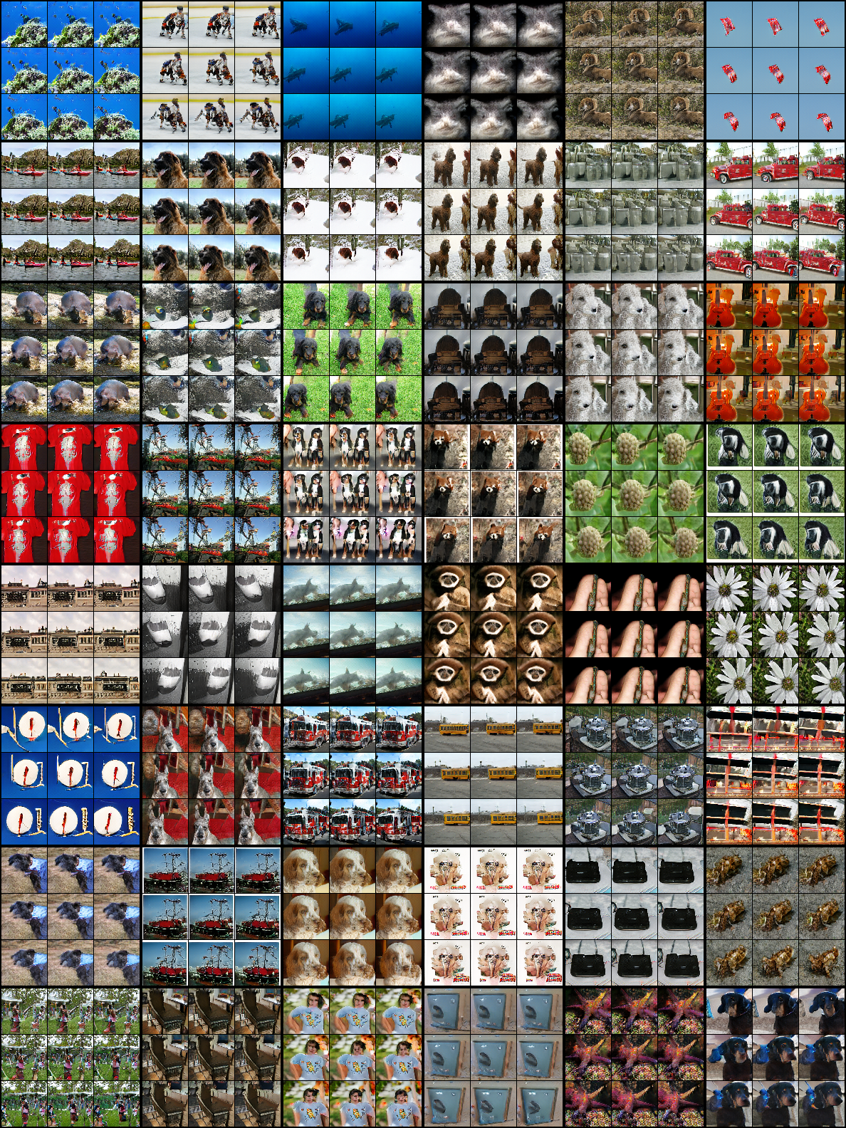
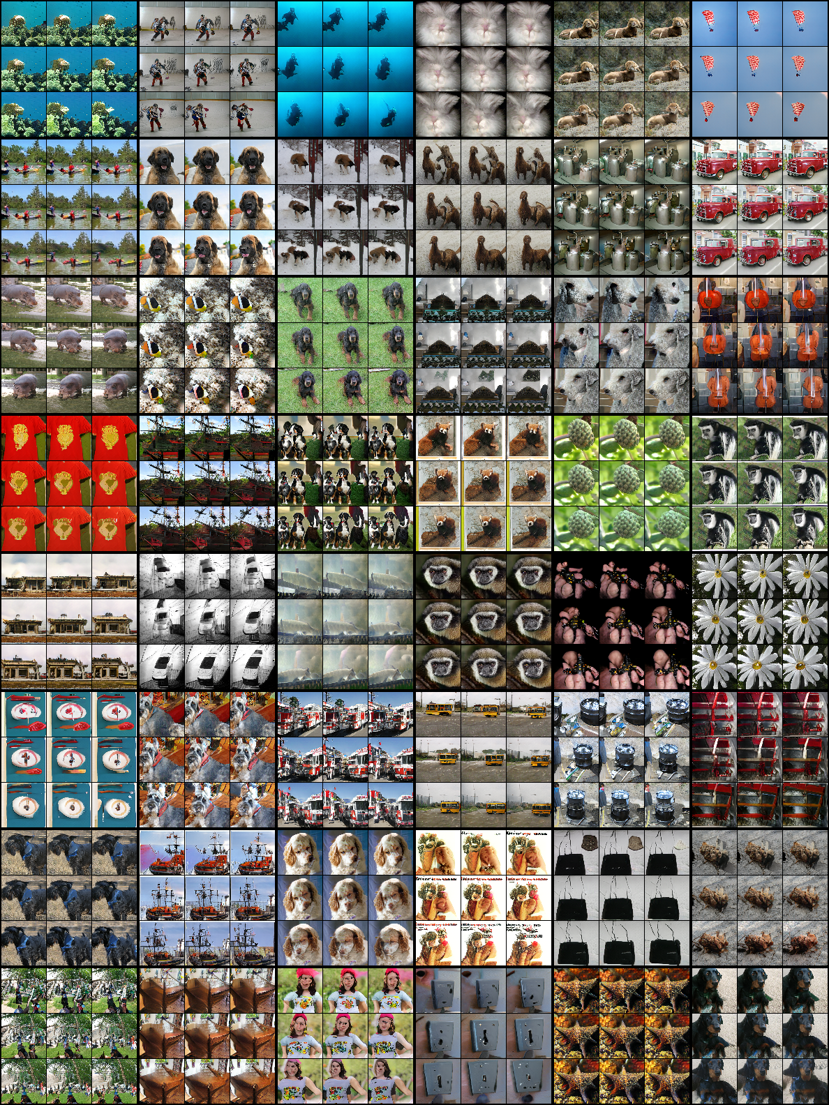
Next, we explore the effects of resampling generator noise. The generator takes as input a Gaussian noise vector, in addition to the logit vector from the pretrained classifier. The noise primarily captures non-semantic properties (Figure 3, 4), mostly small changes in shape, pose, size, and position. These properties reflect information that the classifier has discarded from the logit vector because the generative model considers all of them to be sensible reconstructions of the same logit vector. One particularly interesting invariance is left-right mirroring; our model frequently generates horizontal flips of an image, but not vertical flips. For example, the dog’s body is sometimes on the left and sometimes on the right of the face. We do note, however, that the noise resampling has a greater effect on the non-robust model than on the robust model. This is easily seen in Figure 5, where we linearly interpolate between two noise samples. The robust model is much more stable along the axis of interpolation. We provide many more examples in the Supplementary Materials.

Figure 3: Variation in reconstructions due to noise resampling for Robust ResNet-152. The upper-left tile is the input.

Figure 4: Variation in reconstructions due to noise resampling for non-robust ResNet-152. The upper-left tile is the input.

Figure 5: Noise interpolation for robust (left) and non-robust (right) ResNet-152. We linearly interpolate between random noise vectors. The top-left image corresponds to one noise sample, the lower-right corresponds to another, and all others are linear interpolates arranged left-to-right, top-to-bottom. We find that the reconstruction varies significantly less across noise inputs for the robust model.

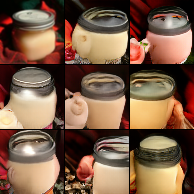
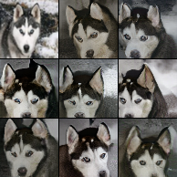
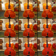
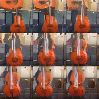
It is interesting to observe invariances being captured in the logits and the generator recovering them via resampled input noises. However, more subtle invariances may not be captured if the discriminator has not learned to look for certain forms of variation as a cue.

5.4 Reconstructing incorrectly classified images

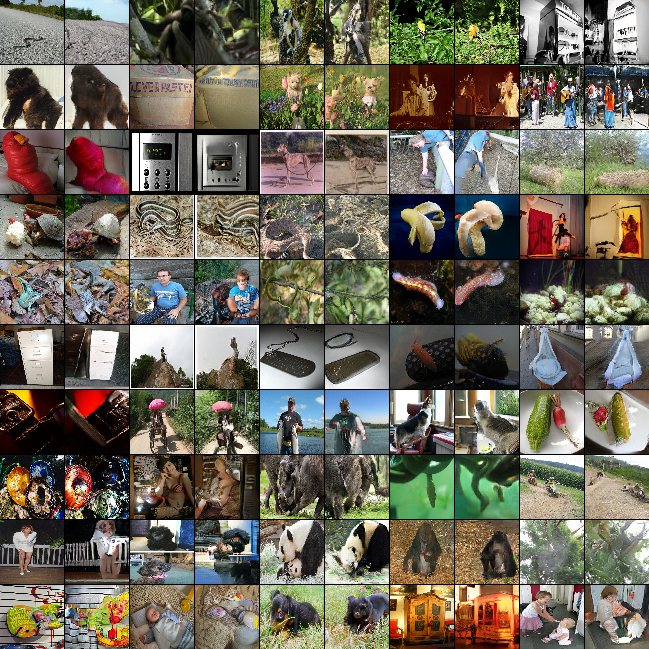
The samples we show in Figure 1 are of correctly classified images. Does the correctness of classification have a significant impact on the nature of reconstruction? If a sample is misclassified because the net ‘sees’ a sample as belonging to a different class, the reconstructions may reveal a categorical shift to the incorrect class. One might therefore expect reconstructions of correctly classified samples to be more veridical than those of incorrectly classified samples. Figure 6 shows that even incorrectly classified samples from the ImageNet test set are faithfully reconstructed. With this, we infer that incorrect classifications are due to the network drawing flawed decision boundaries rather than a semantically flawed embedding. We provide more samples for both the robust and non-robust models in the Supplementary Materials.

Figure 6: Reconstruction of incorrectly classified samples using robust ResNet-152. Surprisingly, even incorrectly classified samples are reconstructed faithfully.

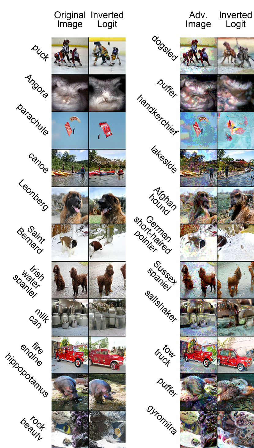
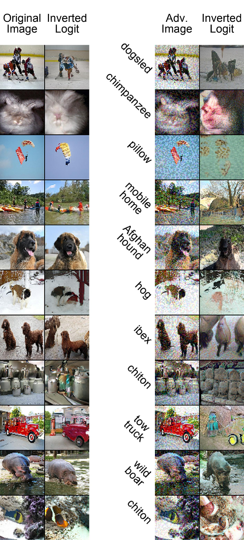
We turn now to another kind of incorrectly classified sample: adversarial examples (Goodfellow et al.,, 2015), small perturbed version of correctly classified images that result in incorrect classification. We use FGSM (Goodfellow et al.,, 2015) to generate adversarial examples, with attack strength $\epsilon=0.1$, meaning that no pixel deviates by more than $\epsilon$ from the source image. Figure 7 shows the original and adversarial images alongside their reconstructions for the robust (left two columnns) and non-robust (right two columns) ResNet models. The correct and incorrect labels are shown beside the images. We selected images for which successful attacks could be found for both robust and non-robust models. Unsurprisingly, the robust model is less sensitive to attacks. Whereas reconstructions of adversarial images in the robust model appear not to lose significant fidelity relative to reconstructions of the original images, the same is not entirely true for the non-robust model. Take the fire engine (3rd row from the bottom) as an example. The adversarial attack leads to a reconstruction in which the vehicle changes color and shape and no longer looks like a fire engine. For the robust model, the adversarial images seem to be reconstructed about as well as ordinary incorrectly classified images (Figure 6); in both cases, visual elements and shapes remain largely intact despite incorrect classification.

(a) Robust

(b) Non-robust

Figure 7: Reconstructions of adversarially attacked images using the FGSM method (Goodfellow et al.,, 2015). Each column of image pairs consists of the input and reconstructed image. The left two columns are from robust ResNet and the right two columns non-robust ResNet. Each pair of columns consists of the original and adversarial images and reconstructions. The true labels are on the very left, and the predicted labels after attack are also shown.

5.5 Logit manipulations

In this section, we explore how three manipulations of the logits affect reconstructions: logit shifting, in which a constant is added to each element of the logit vector; logit scaling, in which each element of the logit vector is multiplied by a constant; and logit perturbation in which i.i.d. Gaussian noises are added to each element of the logit vector. We hold the noise input of the generator constant when manipulating the logit for each sample.

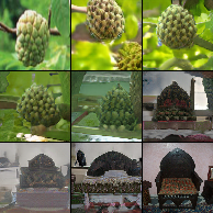
Figure 8a illustrates logit shifting. The five columns are reconstructions of an original image (left side of Figure) with each logit in the vector shifted by a constant. The upper and lower sets of images correspond to robust and standard (non-robust) ResNet-152 models. For robust ResNet-152, the constants for the five columns are $-0.30$, $-0.15$, $0.0$, $0.15$, and $0.30$; for standard ResNet-152, the constants are $-0.1$, $-0.05$, $0.0$, $0.05$, and $0.1$. For larger shifts, reconstructions from standard ResNet lose meaningful contents.

For the robust model, the manipulation primarily affects contrast and sharpness of the reconstructed image but also has subtle effects on shape. For example, in the hockey scene, the three players appear to morph into one with larger shifts. The effect is much less pronounced in the non-robust model, where there are some color changes with positive shifts and content suppression for large negative shifts.

Because a softmax classifier’s output is invariant to logit shifting (the shifts are normalized out), there is no training pressure for the classifier to show any systematic relationship between image features and logit shifts. It must thus be an inductive bias of the training procedure that image contrast and sharpness is reflected on offsets to the logits (Scott et al.,, 2021). We refer the reader to the Supplementary Materials for additional experimental support for the hypothesis suggested by the reconstructions. We show that directly manipulating brightness of an image results in shifted robust logits.

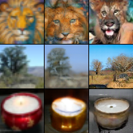
Figure 8b illustrates logit scaling. The five columns are reconstructions with each logit in the vector scaled by a constant, where the constants for the five columns are $10^{-0.3}$, $10^{-0.15}$, $10^{0}$, $10^{0.15}$, and $10^{0.3}$. Surprisingly, for the robust model this manipulation also affects reconstruction contrast and sharpness, almost exclusively. Scaling affects the output confidence distribution: the larger the scaling factor, the more binary model outputs become. Sensibly, the robust classifier has lower confidence for blurry low contrast images. The scaling manipulation appears to affect only contrast and sharpness. During training, the classifier loss is sensitive to changes in the logit scale. Consequently it’s somewhat surprising that scale encodes only contrast and sharpness, and content is well preserved across scale changes. The robust classifier appears to use the embedding direction to represent image content.

In the non-robust model, apart from the extreme ends of the scaling, there is no significant change in brightness. Furthermore, unlike in the robust model, there do seem to be slight changes in content. For example, the coral reef in the top row changes shape. Therefore, for non-robust classifiers, embedding direction and scale encode content.

Figure 8: Reconstructions formed by shifting, scaling, and perturbing logits. The upper set of images is from robust ResNet-152 logits; the lower set is from standard ResNet-152 logits.

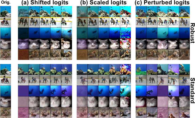
In Figure 8c, we show reconstructions in which the the logits are perturbed by i.i.d. Gaussian noise $\mathcal{N}(\mu=0,\sigma^{2}=0.55)$. For both robust and non-robust models, image content is affected by noise. For the robust model, the content is not so much affected that one could not group together the reconstructions from the same underlying logit vector. However, for the non-robust model the content changes are much larger; indicating that non-robust logits are much more tightly grouped in the output space. We verify this quantitatively by selecting 10 random classes and computing per-class means of validation sample logit vectors. We then measure $l_{2}$ distances between samples from each class to their class mean. For the non-robust model, the mean $l_{2}$ distance is $42.33$, compared to $43.78$ for the robust model, supporting the hypothesis that non-robust logits are grouped more tightly. We note that noise added to the logits has a different effect than providing noise sample $\epsilon$ to the generator. Additive logit noise changes content, whereas $\epsilon$ primarily affects pose and location.

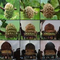
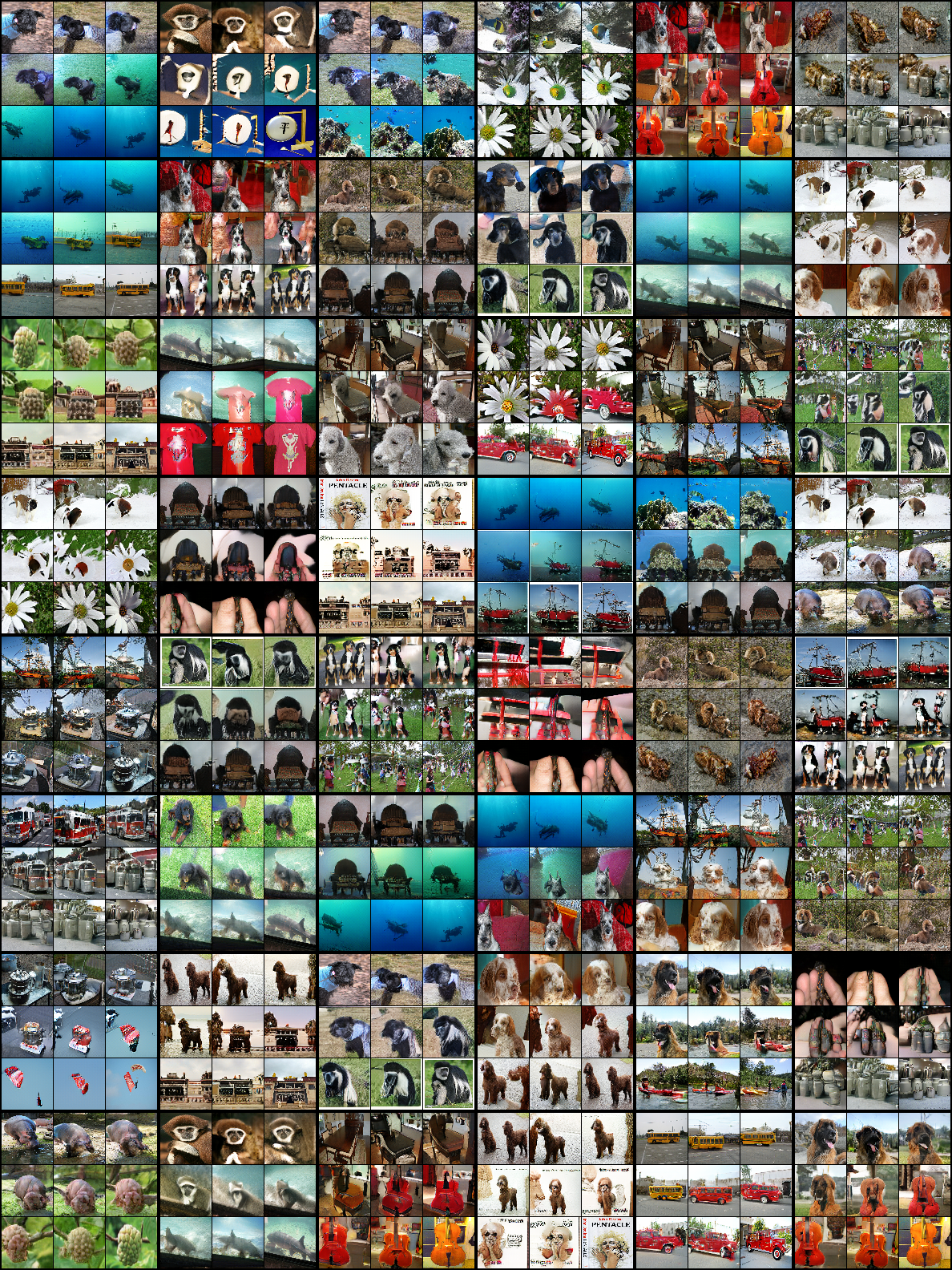
Given the similarity of reconstructions from nearby points in logit space, we also explored the effect of interpolating between the logit vectors of two distinct images. Figure 9 shows two sample reconstruction sequences, formed by linear interpolation between logit vectors, one from the robust model and one from the non-robust model. Although we observe a smooth semantic continuum in which natural looking images are obtained at each interpolation point for both, the robust model has a smoother sequence. We show many more examples in the supplementary materials. Other researchers studying image reconstruction from logits have also observed smooth interpolations (e.g., Dosovitskiy and Brox, 2016a, ), though we appear to be the first to show more organization in the space for robust models.

Figure 9: We compare non-robust logit interpolation (left) and robust logit interpolation (right). The upper left and lower right images in each block are from the ImageNet test set. The intermediate images are obtained by reconstructing interpolations between the logit vectors of these two images.

5.6 Reconstructing out-of-distribution data

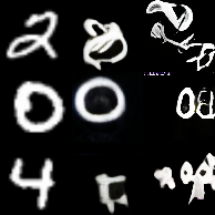
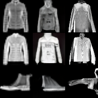
To further understand how classifiers behave on out-of-distribution (OOD) data, we reconstruct samples from non-Imagenet datasets using a model trained on ImageNet. Both the classifier used to construct the logits and the inversion model are trained on ImageNet. ImageNet pre-training for transfer learning is an extremely common and successful method, so it’s natural to ask what about the target dataset is embedded in the features. In Figure 10, we compare the robustly trained ResNet-152 with the standard one on CIFAR-100 (Krizhevsky,, 2009), MNIST (LeCun et al.,, 2010), and FashionMNIST (Xiao et al.,, 2017). It is notable that the robust model offers substantially better reconstructions than the non-robust model. This ability to encode OOD data strongly supports claims of Salman et al., (2020) that robust features are better for transfer learning.

Figure 10: Reconstruction of CIFAR-100, MNIST, and FashionMNIST images with a model trained on ImageNet. The left column is input, middle is Robust ResNet-152 reconstruction, right is standard ResNet-152 reconstruction.

6 Discussion

We summarize our results as follows.

• We obtain remarkably high fidelity reconstructions, which allow the object class to be determined as well as visual detail orthogonal to the class label. In contrast to current state-of-the-art reconstruction methods (Dosovitskiy and Brox, 2016a, ; Engstrom et al.,, 2019), our model preserves global coherence as well as local features.

• Subjectively, robust ResNet produces better reconstructions than non-robust ResNet, suggesting that the adversarial training procedure is effective in preserving features that human observers identify as salient in an image, even if non-class-related.

• Architecture matters. ResNet seems to better preserve visual information than Inception. It seems likely that the short circuit linear connections of ResNet allow low level information to be propagated forward.

• We do not see a qualitative difference in reconstruction fidelity for incorrectly classified images.

• For a robust ResNet-152, both logit shifts and rescaling have have a similar effect—they influence the contrast, sharpness, and brighness of reconstructions. The relationship for non-robust ResNet is similar but weaker.

• The correspondence between logit space and image space is smooth, such that small perturbations to the logits yield small perturbations to reconstructions, and interpolating between logits produces reasonable image interpolations. The interpolation produces a smoother sequence for the robust model.

• The robust ResNet-152 encodes OOD data such as CIFAR and MNIST much more faithfully than non-robust ResNet-152, giving a clue as to why robust models are better for transfer learning.

The degree to which the logit vector is invertible seems quite surprising. After all, perfectly discriminative networks should retain only class-relevant information and should be invariant to differences among instances of a class.

Future work should focus on how to leverage what we learn to design better systems. If robust classifiers result in more invertible features, is it also true that invertible features result in more robust classifiers? Can we use decoded interpolated logits as a form of semantic MixUp (Zhang et al.,, 2017)? Additionally, it would be interesting to inspect and analyze inversions from alternative architechtures such as Vision Transformers (Dosovitskiy et al.,, 2020) and MLP-Mixers (Tolstikhin et al.,, 2021).

We hope that these questions inspire further work which improves learning systems.

7 Acknowledgements

The authors thank Alexey Dosovitskiy for helpful feedback on an earlier draft of this manuscript. The authors also thank the Boston University IVC group for feedback prior to submission. Piotr Teterwak was partially supported by the DARPA XAI program.

8 Noise resampling

In Figures 11 and 12, we provide additional noise resampling results for both robust and non-robust models. For each block of 9 images, the upper left is the input to the classifier. The next 8 are the same logits with different noise vectors fed into the generator.

Figure 11: Additional noise resamplings for the robust ResNet-152 on randomly chosen images from the ImageNet validation set.

Figure 12: Additional noise resmaplings for the non-robust ResNet-152.

9 Interpolations between logits

In Figures 13 and 14 and we interpolate between two logits of two vectors linearly. We find robust models to give a smoother sequence.

Figure 13: Linear interpolations between two logit vectors for the robust ResNet-152. Upper-left and lower-right are ground truth images.

Figure 14: Linear interpolations between two logit vectors for the non-robust ResNet-152. Upper-left and lower-right are ground truth images.

10 Interpolations between noise vectors

In Figures 15 and 16 and we interpolate between two noise vectors linearly. We find that the robust model has a smaller semantic difference between the two endpoints.

Figure 15: Linear interpolations between two noise inputs for the robust ResNet-152

Figure 16: Linear interpolations between two noise inputs for the non-robust ResNet-152

11 Reconstructing Incorrectly Classified Images

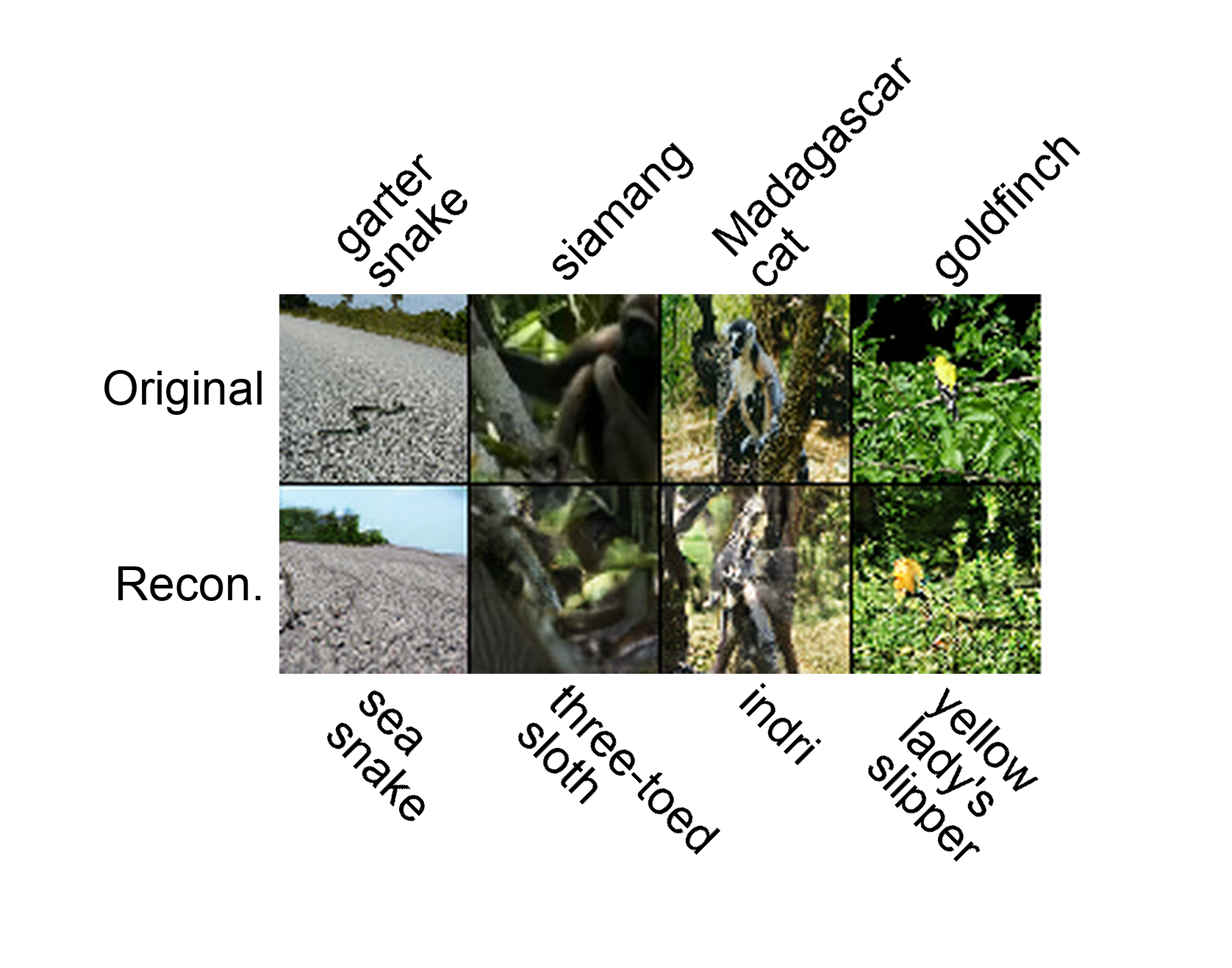
In figures 17 and 18 we show additional examples for incorrectly classified samples. We find that even for incorrectly classified samples, reconstructions are of high quality.

Figure 17: Reconstructions of incorrectly classified images from the robust ResNet-152.

Figure 18: Reconstructions of incorrectly classified images from the non-robust ResNet-152.

12 Iterative Stability

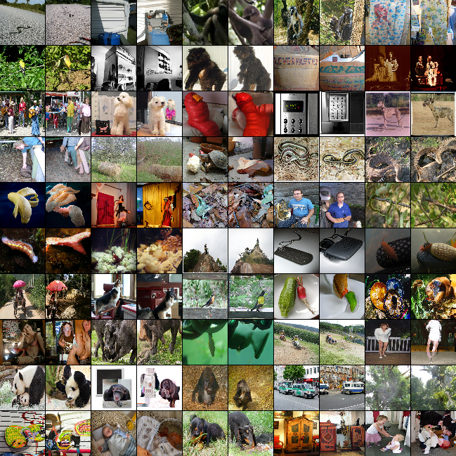
We explore iterative stability of the model; if we pass the reconstructed sample back through the classifier, how often does it predict the same class as the ground truth image? The results are much different for the robust and non-robust models. We take 500 samples from 50 classes of ImageNet for this experiment. For the robust model; if the ground truth sample was correctly classified, the reconstruction is classified identically as the ground truth 54% of the time. If the ground truth was incorrectly classified, the reconstruction is classified identically as the ground truth 35% of the time. There is a substantial difference between correctly classified samples, despite qualitative observations that reconstructions are similarly good for both. The results for the non-robust model are 49.3% and 29.9% respectively. The robust model is more stable, implying that the inversion model is better at preserving features used for classification with the robust model.

13 Analysis of scale and shift effects

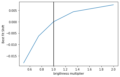
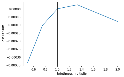
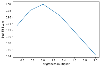
In the main paper, we show that manipulating logits before they are input to inversion model resulted in systematic changes; both scale and shift seemed to encode brightness for the robust ResNet-152 model, while it didn’t have as pronounced an effect on the non-robust model. Here, we show exactly this experimentally for shifts. We start with a batch of images, and then multiply its pixel values by a fixed value to adjust the brightness. Then for each brightness-adjusted image, we compute robust logits. We then find a best-fit shift to get back to the non-brightness adjsuted logits. In other words, we fit the shift parameter in the mode.: $logits_{original}=logits_{brightness-adjusted}+shift$. We do this independently for each image, and report the mean across brightness factors in Figure 19 We find that as the brightness increases , the best-shift does as well. This verifies the finding in the main paper. However, for the non-robust model, the expected shift peaks and then decreases, shown in 20.

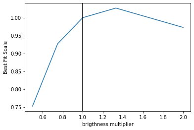
For scale, we perform a similar experiment, except we fit the scale in the model $logits_{original}=logits_{brightness-adjusted}*scale$. We find that the relationship for scale is weaker than for shift. However, locally around the identity transform, there is still a positive relationship between scale and brightness for the robust ResNet-152 (Figure 21); the best-fit scale peaks at a greater brightness than the identity transform. On the other hand, for the non-robust ResNet-152 (Figure 22), the identity transform represents the peak expected scale of 1.

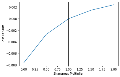
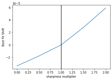
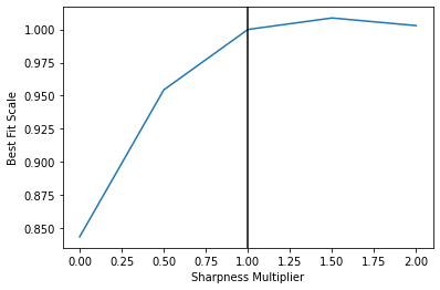
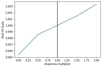
We repeat the experiment for image sharpness manipulations. Image sharpness of 0 means a smoothed image, while image sharpness of 2 means a sharpened image. We show results for the Robust ResNet-152 in Figures 23 and 25, and non-robust ResNet-152 in Figures 24 and 26.

We find that in both models, best-fit scale and shift positively correlate with sharpness. However, for the Robust model, the magnitudes of expected scales and shifts is much much larger.

Figure 19: Plotting best-fit shifts vs. brightness factor for Robust ResNet-152. As brightness increases, so does expected shift. Brightness factor of 1 corresponds to the identity function, so expected shift is 0, this is represented by the vertical line.

Figure 20: Plotting best-fit shifts vs. brightness factor, for non-robust ResNet-152. There is a much weaker relationship than for the robust ResNet-152 model. Brightness factor of 1 corresponds to the identity function, so expected shift is 0, this is represented by the vertical line.

Figure 21: Plotting best-fit scales vs. brightness factor, for robust ResNet-152. Brightness factor of 1 corresponds to the identity function, this is represented by the vertical line. Locally, around this line, there is a positive relationship between scale and brightness.

Figure 22: Plotting best-fit scales vs. brightness factor, for non-robust ResNet-152. Brightness factor of 1 corresponds to the identity function, this is represented by the vertical line.Locally, around this line, there is no positive relationship between scale and brightness.

Figure 23: Plotting best-fit shifts vs. sharpness factor, for Robust ResNet-152. Sharpness factor of 1 corresponds to the identity function, so expected shift is 0, this is represented by the vertical line.

Figure 24: Plotting best-fit shifts vs. sharpness factor, for non-robust ResNet-152. Sharpness factor of 1 corresponds to the identity function, so expected shift is 0, this is represented by the vertical line. There is a positive relationship.

Figure 25: Plotting best-fit scales vs. sharpness factor, for robust ResNet-152. Brightness factor of 1 corresponds to the identity function, this is represented by the vertical line. Although there is a positive relationship, the best fit shifts are much smaller magnitude.

Figure 26: Plotting best-fit scales vs. sharpness factor, for non-robust ResNet-152. Sharpness factor of 1 corresponds to the identity function, this is represented by the vertical line. There is a strong relationship. Again, although there is a positive relationship, the expected scales magnitudes are much smaller than for the robust model.

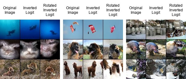
13.1 Effect of image-space rotations on reconstructions

In the main paper, we explored manipulations of the logits, i.e., the input to the decoder. With logit manipulations, we can infer what aspects of the image will cause the classifier to produce corresponding variation in the logits. In this section, we directly manipulate images, in order to determine whether the robust classifier preserves information about the manipulation and whether the decoder can recover the original image. The particular manipulation we study is rotation of the image by 90 degrees. Figure 27 shows an original image, the reconstruction of this image from the robust logits, and the reconstruction of this image rotated by 90 degrees. To make it easier to compare images, we counter-rotate the latter reconstruction so that it will be identical to the original image if it is reconstructed veridically. We observe some signal in the rotated reconstruction, but clearly there is degradation. For example, animals—which are nearly always upright in ImageNet—are horribly distorted. The classifier and/or decoder do not appear to generalize well outside of the data distribution they were trained on (i.e., upright data). Interestingly, textures are fairly well reconstructed, such as the background brush in the third row, left triplet, which makes sense given that textures tend not to have a reliable orientation in the natural world.

Figure 27: Reconstruction of rotations. We compare images encoded with Robust ResNet-152 (left column) to the their reconstructions (middle), and reconstructions of the same image rotated by 90 degrees (right). We counter-rotate the reconstruction for ease of comparison. The rotated samples reconstruct textures reasonably well but objects are horribly disfigured.

14 Training Details

14.1 Network Architectures

We use a BigGAN generator configured for 64x64 images. The layer configuration is listed below. Each residual block contains 3 conditional-batch norms and a single 2x upsampling operation, in addition to convolutions and non-linearities. We use hierarchical noise input, detailed in (Brock et al.,, 2018). For more details, please see (Brock et al.,, 2018) and the compare_gan codebase.

Layer	Out Resolution	Out Channels
Linear(noise)	4	1536
Residual Block Upsampling	8	1536
Residual Block Upsampling	16	768
Residual Block Upsampling	32	384
Residual Block Upsampling	64	192
Non-local block (self-attention)	64	192
BN, ReLU, and Conv	64	3
Tanh	64	3

Table 3: Generator architecture

Similarly, we use the BigGAN discriminator. There are 4 resblock with downsampling, and one without. The proection discriminator, described in the main paper, comes at the end. Again, for more details, please see (Brock et al.,, 2018) and the compare_gan codebase.

Layer	Out Resolution	Out Channels
ResBlock Down	32	192
Non-local block (self-attention)	32	192
ResBlock Down	16	384
ResBlock Down	8	768
ResBlock Down	4	1536
ResBlock	4	1536
ReLU, Global Sum pooling	1	1536
Conditional Projection	1	1

Table 4: Discriminator architecture

We train with the Adam optimizer with $\beta_{1}$ set to 0 and $\beta_{2}$ set to 0.999, and a learning rate of $0.0001$ for the generator and $0.0005$ for the discriminator. We take 2 discriminator steps for every generator step. We initialize weights orthognally, and use spectral norm in both the generator and discriminator. For more details, see below.

14.2 Training Configuration

Below, the exact configuration used for the inversion models in the paper. It can be used directly with the compare_gan code.

# Parameters for AdamOptimizer:
# ===============================================
AdamOptimizer.beta1 = 0.0
AdamOptimizer.beta2 = 0.999

# Parameters for D:
# ===============================================
D.spectral_norm = True

# Parameters for dataset:
# ===============================================
dataset.name = ’imagenet_64’

# Parameters for resnet_biggan.Discriminator:
# ===============================================
resnet_biggan.Discriminator.project_labels = True

# Parameters for eval_z:
# ===============================================
eval_z.distribution_fn = @tf.random.stateless_normal

# Parameters for G:
# ===============================================
G.batch_norm_fn = @conditional_batch_norm
G.spectral_norm = True

# Parameters for resnet_biggan.Generator:
# ===============================================
resnet_biggan.Generator.embed_labels = True
resnet_biggan.Generator.hierarchical_z = True

# Parameters for loss:
# ===============================================
loss.fn = @hinge

# Parameters for ModularGAN:
# ===============================================
ModularGAN.conditional = True
ModularGAN.d_inputs = [’label’]
ModularGAN.d_lr = 0.0005
ModularGAN.d_optimizer_fn = @tf.train.AdamOptimizer
ModularGAN.g_inputs = [’label’]
ModularGAN.g_lr = 0.0001
ModularGAN.g_optimizer_fn = @tf.train.AdamOptimizer
ModularGAN.g_use_ema = True

# Parameters for options:
# =================================================
options.architecture = ’resnet_biggan_arch’
options.batch_size = 2048
options.disc_iters = 2
options.gan_class = @ModularGAN
options.lamba = 1
options.training_steps = 250000
options.z_dim = 120

# Parameters for penalty:
# =================================================
penalty.fn = @no_penalty

# Parameters for run_config:
# =================================================
run_config.iterations_per_loop = 500
run_config.save_checkpoints_steps = 2500
run_config.tf_random_seed = 8

# Parameters for spectral_norm:
# =================================================
spectral_norm.singular_value = ’auto’

# Parameters for standardize_batch:
# =================================================
standardize_batch.decay = 0.9
standardize_batch.epsilon = 1e-05
standardize_batch.use_moving_averages = False

# Parameters for weights:
# =================================================
weights.initializer = ’orthogonal’

# Parameters for z:
# =================================================
z.distribution_fn = @tf.random.normal

References

- Brock et al., (2018) Brock, A., Donahue, J., and Simonyan, K. (2018). Large scale gan training for high fidelity natural image synthesis. In International Conference on Learning Representations.
- De Vries et al., (2017) De Vries, H., Strub, F., Mary, J., Larochelle, H., Pietquin, O., and Courville, A. C. (2017). Modulating early visual processing by language. In Advances in Neural Information Processing Systems, pages 6594–6604.
- Dosovitskiy et al., (2020) Dosovitskiy, A., Beyer, L., Kolesnikov, A., Weissenborn, D., Zhai, X., Unterthiner, T., Dehghani, M., Minderer, M., Heigold, G., Gelly, S., et al. (2020). An image is worth 16x16 words: Transformers for image recognition at scale. arXiv preprint arXiv:2010.11929.
- (4) Dosovitskiy, A. and Brox, T. (2016a). Generating images with perceptual similarity metrics based on deep networks. In Advances in neural information processing systems, pages 658–666.
- (5) Dosovitskiy, A. and Brox, T. (2016b). Inverting visual representations with convolutional networks. In Proceedings of the IEEE conference on computer vision and pattern recognition, pages 4829–4837.
- Dumoulin et al., (2016) Dumoulin, V., Shlens, J., and Kudlur, M. (2016). A learned representation for artistic style. arXiv preprint arXiv:1610.07629.
- Engstrom et al., (2019) Engstrom, L., Ilyas, A., Santurkar, S., Tsipras, D., Tran, B., and Madry, A. (2019). Learning perceptually-aligned representations via adversarial robustness. arXiv preprint arXiv:1906.00945.
- Goodfellow et al., (2015) Goodfellow, I. J., Shlens, J., and Szegedy, C. (2015). Explaining and harnessing adversarial examples. In ICLR.
- He et al., (2016) He, K., Zhang, X., Ren, S., and Sun, J. (2016). Deep residual learning for image recognition. In Proceedings of the IEEE conference on computer vision and pattern recognition, pages 770–778.
- Jia et al., (2014) Jia, Y., Shelhamer, E., Donahue, J., Karayev, S., Long, J., Girshick, R., Guadarrama, S., and Darrell, T. (2014). Caffe: Convolutional architecture for fast feature embedding. arXiv preprint arXiv:1408.5093.
- Johnson et al., (2016) Johnson, J., Alahi, A., and Fei-Fei, L. (2016). Perceptual losses for real-time style transfer and super-resolution. In European Conference on Computer Vision.
- Krizhevsky, (2009) Krizhevsky, A. (2009). Learning multiple layers of features from tiny images. Technical report.
- LeCun et al., (2010) LeCun, Y., Cortes, C., and Burges, C. (2010). Mnist handwritten digit database. ATT Labs [Online]. Available: http://yann.lecun.com/exdb/mnist, 2.
- Madry et al., (2017) Madry, A., Makelov, A., Schmidt, L., Tsipras, D., and Vladu, A. (2017). Towards deep learning models resistant to adversarial attacks. arXiv preprint arXiv:1706.06083.
- Mahendran and Vedaldi, (2015) Mahendran, A. and Vedaldi, A. (2015). Understanding deep image representations by inverting them. In Proceedings of the IEEE conference on computer vision and pattern recognition, pages 5188–5196.
- Mirza and Osindero, (2014) Mirza, M. and Osindero, S. (2014). Conditional generative adversarial nets. arXiv preprint arXiv:1411.1784 [cs.LG].
- Miyato and Koyama, (2018) Miyato, T. and Koyama, M. (2018). cGANs with projection discriminator. In International Conference on Learning Representations.
- Nash et al., (2019) Nash, C., Kushman, N., and Williams, C. K. (2019). Inverting supervised representations with autoregressive neural density models. In The 22nd International Conference on Artificial Intelligence and Statistics, pages 1620–1629. PMLR.
- Park et al., (2019) Park, T., Liu, M.-Y., Wang, T.-C., and Zhu, J.-Y. (2019). Semantic image synthesis with spatially-adaptive normalization. In Proceedings of the IEEE Conference on Computer Vision and Pattern Recognition.
- Qin et al., (2019) Qin, C., Martens, J., Gowal, S., Krishnan, D., Dvijotham, K., Fawzi, A., De, S., Stanforth, R., and Kohli, P. (2019). Adversarial robustness through local linearization. In Advances in Neural Information Processing Systems, pages 13824–13833.
- Rombach et al., (2020) Rombach, R., Esser, P., and Ommer, B. (2020). Making sense of cnns: Interpreting deep representations & their invariances with inns. arXiv preprint arXiv:2008.01777.
- Russakovsky et al., (2015) Russakovsky, O., Deng, J., Su, H., Krause, J., Satheesh, S., Ma, S., Huang, Z., Karpathy, A., Khosla, A., Bernstein, M., et al. (2015). Imagenet large scale visual recognition challenge. International journal of computer vision, 115(3):211–252.
- Salman et al., (2020) Salman, H., Ilyas, A., Engstrom, L., Kapoor, A., and Madry, A. (2020). Do adversarially robust imagenet models transfer better? arXiv preprint arXiv:2007.08489.
- Santurkar et al., (2019) Santurkar, S., Tsipras, D., Tran, B., Ilyas, A., Engstrom, L., and Madry, A. (2019). Image synthesis with a single (robust) classifier. arXiv preprint arXiv:1906.09453.
- Scott et al., (2021) Scott, T. R., Gallagher, A. C., and Mozer, M. C. (2021). von Mises-Fisher loss: An exploration of embedding geometries for supervised learning. arXiv preprint arXiv:2103.15718 [cs.LG].
- Shocher et al., (2020) Shocher, A., Gandelsman, Y., Mosseri, I., Yarom, M., Irani, M., Freeman, W. T., and Dekel, T. (2020). Semantic pyramid for image generation. In Proceedings of the IEEE/CVF Conference on Computer Vision and Pattern Recognition (CVPR).
- Szegedy et al., (2016) Szegedy, C., Vanhoucke, V., Ioffe, S., Shlens, J., and Wojna, Z. (2016). Rethinking the inception architecture for computer vision. In Proceedings of the IEEE conference on computer vision and pattern recognition, pages 2818–2826.
- Teterwak et al., (2019) Teterwak, P., Sarna, A., Krishnan, D., Maschinot, A., Belanger, D., Liu, C., and Freeman, W. T. (2019). Boundless: Generative adversarial networks for image extension. In The IEEE International Conference on Computer Vision (ICCV).
- Tolstikhin et al., (2021) Tolstikhin, I., Houlsby, N., Kolesnikov, A., Beyer, L., Zhai, X., Unterthiner, T., Yung, J., Keysers, D., Uszkoreit, J., Lucic, M., et al. (2021). Mlp-mixer: An all-mlp architecture for vision. arXiv preprint arXiv:2105.01601.
- Xiao et al., (2017) Xiao, H., Rasul, K., and Vollgraf, R. (2017). Fashion-mnist: a novel image dataset for benchmarking machine learning algorithms. CoRR, abs/1708.07747.
- Zeiler and Fergus, (2014) Zeiler, M. D. and Fergus, R. (2014). Visualizing and understanding convolutional networks. In European conference on computer vision, pages 818–833. Springer.
- Zhang et al., (2017) Zhang, H., Cisse, M., Dauphin, Y. N., and Lopez-Paz, D. (2017). mixup: Beyond empirical risk minimization. arXiv preprint arXiv:1710.09412.
- Zhang et al., (2018) Zhang, R., Isola, P., Efros, A. A., Shechtman, E., and Wang, O. (2018). The unreasonable effectiveness of deep features as a perceptual metric. In Proceedings of the IEEE conference on computer vision and pattern recognition, pages 586–595.
- Zhang et al., (2016) Zhang, Y., Lee, K., and Lee, H. (2016). Augmenting supervised neural networks with unsupervised objectives for large-scale image classification. In International conference on machine learning, pages 612–621.