Terrain prickliness: theoretical grounds
for high complexity viewsheds

Abstract

An important task in terrain analysis is computing viewsheds. A viewshed is the union of all the parts of the terrain that are visible from a given viewpoint or set of viewpoints. The complexity of a viewshed can vary significantly depending on the terrain topography and the viewpoint position. In this work we study a new topographic attribute, the prickliness, that measures the number of local maxima in a terrain from all possible angles of view. We show that the prickliness effectively captures the potential of 2.5D TIN terrains to have high complexity viewsheds. We present optimal (for 1.5D terrains) and near-optimal (for 2.5D terrains) algorithms to compute it for TIN terrains, and efficient approximate algorithms for raster DEMs. We validate the usefulness of the prickliness attribute with experiments in a large set of real terrains.

1 Introduction

Digital terrain models represent part of the earth’s surface, and are used to solve a variety of problems in geographic information science. An important task is viewshed analysis: determining which parts of a terrain are visible from certain terrain locations. Two points $p$ and $q$ on or above a terrain are mutually visible if the line of sight defined by line segment $\overline{pq}$ does not intersect the interior of the terrain. Given a viewpoint $p$, the viewshed of $p$ is the set of all terrain points that are visible from $p$. Similarly, the viewshed of a set of viewpoints $P$ is defined as the set of all terrain points that are visible from at least one viewpoint in $P$. Viewsheds are useful, for example, in evaluating the visual impact of potential constructions [4], analyzing the coverage of an area by fire watchtowers [15], or measuring the scenic beauty of a landscape [2, 25].

1.1 Discrete and continuous terrain representations

Two major terrain representations are prevalent in GIS. The simplest and most widespread is the raster, or digital elevation model (DEM), consisting of a rectangular grid where each cell stores an elevation. The main alternative is a vector representation, or triangulated irregular network (TIN), where a set of irregularly spaced elevation points are connected into a triangulation. A TIN can be viewed as a continuous $xy$-monotone polyhedral surface in $\mathbb{R}^{3}$. A viewshed in a DEM is the set of all raster cells that are visible from at least one viewpoint. In contrast, a viewshed in a TIN is the union of all parts of triangles that are visible from at least one viewpoint, so it can be seen as a set of polygons.

DEMs are simpler to analyze than TINs and facilitate most analysis tasks. The main advantage of TINs is that they require less storage space. Both models have been considered extensively in the literature for viewshed analysis, see Dean [5] for a complete comparison of both models in the context of forest viewshed. Some studies suggest that TINs can be superior to DEMs in viewshed computations [5], but experimental evidence is inconclusive [23]. This is in part due to the fact that the viewshed algorithms used in [23] do not compute the visible part of each triangle, but only attempt to determine whether each triangle is completely visible. This introduces an additional source of error and does not make use of all the information contained in the TIN.

Figure 1: Part of a TIN with a high-complexity viewshed. The viewpoint (not shown) is placed at the center of projection. The relevant triangles of the TIN are the ones shown, which define $n$ peaks and ridges. The viewshed in this case is formed by $\Theta(n^{2})$ visible regions.

1.2 Viewshed complexity

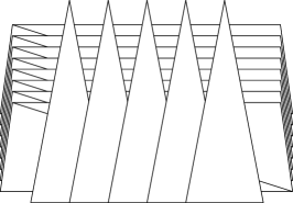
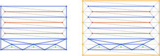
The algorithmic study of viewsheds focuses on two main aspects: the complexity of the viewsheds, and their efficient computation. In this work, we are interested in their complexity. We use the information-theoretic meaning of “complexity”: the complexity of an object is the number of bits needed to represent it in memory. Therefore, in the case of TINs, viewshed complexity is defined as the total number of vertices of the polygons that form the viewshed. In the case of DEMs, there are several ways to measure viewshed complexity. To facilitate comparison between TIN and DEM viewsheds, we convert the visible areas in the raster viewshed to polygons, and define the viewshed complexity as the total number of vertices in those polygons. A typical high-complexity viewshed construction for a TIN is shown schematically in Fig. 1, where one viewpoint would be placed at the center of projection, and both the number of vertical and horizontal triangles is $\Theta(n)$, for $n$ terrain vertices. The vertical peaks form a grid-like pattern with the horizontal triangles, leading to a viewshed with $\Theta(n^{2})$ visible triangle pieces.

While a viewshed can have high complexity, this is expected to be uncommon in real terrains [1]. There have been attempts to define theoretical conditions for a (TIN) terrain that guarantee, among others, that viewsheds cannot be that large. For instance, Moet et al. [22] showed that if terrain triangles satisfy certain “realistic” shape conditions, viewsheds have $O(n\sqrt{n})$ complexity. De Berg et al. [1] showed that similar conditions guarantee worst-case expected complexity of $\Theta(n)$ when the vertex heights are subject to uniform noise.

1.3 Viewsheds and peaks

The topography of the terrain has a strong influence on the potential complexity of the viewshed. To give an extreme example, in a totally concave terrain, the viewshed of any viewpoint will be the whole terrain, and has a trivial description. Intuitively, to obtain a high complexity viewshed as in Fig. 1, one needs a large number of obstacles obstructing the visibility from the viewpoint, which requires a somewhat rough topography.

In fact, it is well-established that viewsheds tend to be more complex in terrains that are more “rugged” [16]. This leads to the natural question of which terrain characteristics correlate with high complexity viewsheds. Several topographic attributes have been proposed to capture different aspects of the roughness of a terrain, such as the terrain ruggedness index [24], the terrain shape index [20], or the fractal dimension [18]. These attributes focus on aspects like the amount of elevation change between adjacent parts of a terrain, its overall shape, or the terrain complexity. However, none of them is specifically intended to capture the possibility to produce high complexity viewsheds, and there is no theoretical evidence for such a correlation. Moreover, these attributes are locally defined, and measure only attributes of the local neighborhood of one single point. While we can average these measures over the whole terrain, given the global nature of visibility, it is unclear a priori whether such measures are suitable for predicting viewshed complexity. We refer to Dong et al. [6] for a systematic classification of topographic attributes.

Figure 2: Left: a TIN (in $\mathbb{R}^{2}$) with three peaks and one viewpoint ($p$), with a viewshed composed of three parts (visible parts shown orange). Right: transformation of the terrain with no peaks (other than $p$) but the same viewshed complexity. Dotted segments show lines of sight from $p$.

One very simple and natural global measure of the ruggedness of a terrain that is relevant for viewshed complexity is to simply count the number of peaks (i.e., local maxima) in the terrain. It has been observed that areas with higher elevation difference, and hence, more peaks, cause irregularities in viewsheds [11, 15], and this idea aligns with our theoretical understanding: the quadratic example from Fig. 1 is designed by creating an artificial row of peaks, and placing a viewpoint behind them. However, while it seems reasonable to use the peak count as complexity measure, there is no theoretical correlation between the number of peaks and the viewshed complexity. This is easily seen by performing a simple trick: any terrain can be made arbitrarily flat by scaling it in the $z$-dimension by a very small factor, and then it can be rotated slightly. This results in a valid terrain without any peaks, but retains the same viewshed complexity. See Fig. 2 for an example in $\mathbb{R}^{2}$. In fact, viewshed complexity is invariant under affine transformations (i.e., scalings, rotations, and translations) of the terrain: the application of any affine combination to the terrain and the viewpoints results in a viewshed of the same complexity. Hence, any measure that has provable correlation with it must be affine-invariant as well. This is a common problem to establish theoretical guarantees on viewshed complexity, or to design features of “realistic” terrains in general [1, 22]. In fact, it is easy to see that none of the terrain attributes mentioned above is affine-invariant.

1.4 Prickliness

In this work we propose a new topographic attribute: the prickliness. The definition follows directly from the above observations: it counts the number of peaks in a terrain, but does so for every possible affine transformation of the terrain. We first present a definition for TINs, and then we explain how the definition carries over to DEMs.

Let $T$ be a triangulated surface that is $xy$-monotone. Let $A$ be an affine transformation, and let $A(T)$ be the terrain obtained after applying $A$ to $T$. We define $m(A(T))$ to be the number of internal and convex vertices of $T$ that are peaks in $A(T)$. Let ${\cal A}(T)$ be the set of all affine transformations of $T$. We define the prickliness of $T$, $\pi(T)$, to be the maximum number of local maxima over all transformations of $T$; that is, $\pi(T)=\max_{A\in{\cal A(T)}}m(A(T))$. We start by observing that, essentially, the prickliness considers all possible directions in which the number of peaks are counted. Let $\vec{v}$ be a vector in $\mathbb{R}^{3}$. Let $\pi_{\vec{v}}(T)$ be the number of internal and convex vertices of $T$ that are local maxima of $T$ in direction $\vec{v}$; that is, the number of internal and convex vertices of $T$ for which the local neighborhood does not extend further than that vertex in direction $\vec{v}$.

Observation 1.1

$\pi(T)=\max_{\vec{v}}\pi_{\vec{v}}(T)$.

Proof

Clearly, for every vector $\vec{v}$ there exists an affine transformation $A$ such that $m(A(T))=\pi_{\vec{v}}(T)$: take $A$ equal to the rotation that makes $\vec{v}$ vertical. We will show that also for every affine transformation $A$ there exists a vector $\vec{v}$ for which $m(A(T))=\pi_{\vec{v}}(T)$. In particular, this then implies that the maximum value of $m(A(T))$ over all $A$ is equal to the maximum value of $\pi_{\vec{v}}(T)$ over all $\vec{v}$.

Let $A$ be an affine transformation, and let $H$ be the horizontal plane $z=0$. Consider the transformed plane $H^{\prime}=A^{-1}(H)$. Then any vertex of $T$ which has the property that all neighbors are on the same side of $H^{\prime}$ in $T$, will be a local maximum or local minimum in $A(T)$. Now, choose for $\vec{v}$ the vector perpendicular to $H^{\prime}$ and pointing in the direction which will correspond to local maxima.

Figure 3: (left) A TIN $T$, with triangulation edges shown in black, and elevation indicated using colors. (right) A visualization of the prickliness of $T$ as a function of the angles $(\theta,\phi)$ that define each direction (circles indicate contour lines for $\theta$); color indicates prickliness. The maximum prickliness is $8$, attained at a direction of roughly $\theta=13^{\circ}$ and $\phi=60^{\circ}$ (north-east from the origin).

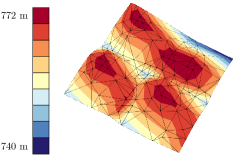
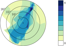
Using this observation, we reduce the space of all affine transformations to the 2-dimensional space of all directions in 3D. Since $T$ is a terrain, for any $\vec{v}$ with a negative $z$-coordinate we have $\pi_{\vec{v}}(T)=0$ by definition, thus the interesting directions reduce to the points on the (positive) unit half-sphere. This provides a natural way to visualize the prickliness of a terrain. Each direction can be expressed using two angles $\theta$ and $\phi$ (i.e., using spherical coordinates), where $\theta$ represents the polar angle and $\phi$ the azimuthal angle. Fig. 3 shows a small terrain and the resulting prickliness, showing a projection of the half-sphere, where each point represents a direction, and its color indicates its prickliness.

DEM terrains

We note that all previous notions easily translate to DEMs. The centers of the DEM cells can be seen as the vertices of the terrain, and every internal vertex of the terrain has eight neighbors given by the cell centers of the eight neighboring cells. Hence, in the definitions for DEMs, the notion of adjacent vertices for TINs is replaced by that of neighbors. A vertex is a local maximum for some affine transformation of the terrain if all of its neighbors have a lower or equal $z$-coordinate. This gives an equivalent definition of $\pi(T)$ when $T$ is a DEM.

In the case of DEMs, the definition of visibility between two points needs to be adapted in order to compute viewsheds. In our experimental work, we rely on the software routines provided by ArgGIS Pro, in particular on their Geodesic Viewshed package. In this package, the visibility between two points is decided as follows. The line of sight between the two points is projected onto the spheroid representing the earth surface, resulting in a ground path. The ground path is sampled with step points with consecutive distance proportional to the DEM cell-size. For each step point, it is checked if the terrain at that point obstructs the line of sight. The two points are considered visible if and only if no obstruction is found. For more details on this we refer to ArcGIS Pro documentation [8].

1.5D TIN terrains

The most widespread terrain model in the computational geometry literature is the TIN (also called polyhedral terrain). Visibility-related questions constitute an important family of problems concerning TIN terrains, but unfortunately some of these problems are quite difficult. For this reason, terrains have also been defined and studied in one dimension less. Standard TINs, as defined earlier in this paper, will be referred as 2.5D TIN terrains. If the dimension is reduced by one, we have 1.5D terrains, which can be seen as graphs of piece-wise linear univariate functions. The simpler structure of 1.5D terrains makes it an interesting intermediate step towards the full understanding of problems in 2.5D TIN terrains. For this reason 1.5D terrains, and in particular visibility problems on them, have been thoroughly studied during the last 15 years. In this work, first we study prickliness in 1.5D because it is conceptually easier, and then we investigate to what extent our results from the 1.5D case give insights into the 2.5D case. This is a common approach in the field.

More formally, a 1.5D TIN terrain is defined as an $x$-monotone polygonal line in $\mathbb{R}^{2}$. In this setting, a viewshed is composed of parts of terrain edges, and the viewshed of one viewpoint can have a complexity that is linear on the number of vertices of the terrain. Prickliness is defined as in the 2.5D case. Additionally, in this case it is also enough to consider all possible directions rather than all possible affine transformations (the proof of Observation 1.1 still applies unchanged). Notice that here directions are not vectors in $\mathbb{R}^{3}$ anymore, but vectors in $\mathbb{R}^{2}$.

1.5 Results and organization

The remainder of this paper is organized as follows.

We start with a theoretical block, composed of Sections 2-5. This block is only concerned with TIN terrains because this is the most interesting model from a theoretical point of view and the one for which viewshed complexity is better understood—recall that there is not a unique way to measure viewshed complexity for DEMs. We study two aspects of prickliness for TIN terrains, first in the easier case of $1.5$D terrains, and then for $2.5$D terrains. In Sections 2-3, we investigate the correlation between the prickliness of a terrain and the maximum complexity of the viewshed of a viewpoint. We show that the prickliness of a $1.5$D terrain and the viewshed complexity of a single viewpoint are not related: we give examples where one is constant and the other is linear. In contrast, unlike other measures of terrain ruggedness, there is a provable correlation between prickliness and viewshed complexity in $2.5$D. In Sections 4-5, we investigate the computational problem of calculating the prickliness of a terrain. We show that the prickliness of a 1.5D or 2.5D TIN terrain can be computed in polynomial time. The algorithm for the 1.5D case is optimal, while the one for the 2.5D case is near-optimal. We also provide an efficient approximate algorithm for 2.5D DEM terrains, which is used in our experiments.

In the second block of the paper, composed of Sections 6-9, we report on experiments that measure the values of distinct topographic attributes (including the prickliness) of real (2.5D) terrains, and analyze their possible correlation with viewshed complexity. From the experiments, we conclude that prickliness provides such a correlation in the case of TIN terrains, while the other measures perform more poorly. The situation for DEM terrains is less clear.

Code

Finally, we provide our code implementing two key algorithms for this work: an algorithm to calculate the prickliness of a TIN terrain (source code available from https://github.com/GTMeijer/Prickliness; archived at swh:1:dir:c360f8c5b838bfe88910d26aad151dee69f69364), and an algorithm to calculate the combined viewshed originating from a set of multiple viewpoints (source code available from https://github.com/GTMeijer/TIN_Viewsheds; archived at swh:1:dir:911b84528046c62ddd56c32905926748dd59791e).

Part I Theoretical results

2 Prickliness and viewshed complexity in 1.5D TIN terrains

The prickliness of a $1.5$D terrain and the viewshed complexity of a single viewpoint do not seem to be related. In order to show it, we need to introduce some notation.

For every internal and convex vertex $v$ in $T$, we are interested in the vectors $\vec{w}$ such that $v$ is a local maximum of $T$ in direction $\vec{w}$. Note that these feasible vectors $\vec{w}$ can be represented as unit vectors, and then the feasible set becomes a region of the unit circle $\mathbb{S}^{1}$, which we denote by $se(v)\subset\mathbb{S}^{1}$. To find $se(v)$, for each edge $e$ of $T$ incident to $v$ we consider the line $\ell$ through $v$ which is perpendicular to $e$. Then we take the half-plane bounded by $\ell$ and opposite to $e$, and we translate it so that its boundary contains the origin. Finally, we intersect this half-plane with $\mathbb{S}^{1}$, which yields a half-circle. We intersect the two half-circles associated to the two edges of $T$ incident to $v$, and obtain a sector of $\mathbb{S}^{1}$. For each direction $\vec{w}$ contained in the sector, the two corresponding edges do not extend further than $v$ in direction $\vec{w}$. Thus, $v$ is a local maxima in direction $\vec{w}$ and this sector indeed represents $se(v)$. See Fig. 4 for an example.

Figure 4: In shaded, $se(v)$ for the corresponding vertices.

Theorem 2.1

There exists a 1.5D terrain $T$ with $n$ vertices and constant prickliness, and a viewpoint on $T$ with viewshed complexity $\Theta(n)$.

Proof

The construction is illustrated in Fig. 5, left. From a point $p$, we shoot $n/2$ rays in the fourth quadrant of $p$ such that the angle between any pair of consecutive rays is $2/n$. On the $i$th ray, there are two consecutive vertices of the terrain, namely, $v_{i}$ and $w_{i}$. The vertices are placed so that $\angle w_{i-1}v_{i}w_{i}=180-3/n$.

Figure 5: Left: terrains with low prickliness can have high viewshed complexity. Right: a vase.

For every $i$, we have that $se(v_{i})$ has angle $3/n$, while $se(w_{i})$ is empty because $w_{i}$ is not convex. Since the angle between $w_{i-1}v_{i}$ and $w_{i}v_{i+1}$ is $2/n$ and the angle between $v_{i}w_{i}$ and $v_{i+1}w_{i+1}$ is also $2/n$, we have that $se(v_{i+1})$ can be obtained by rotating counterclockwise $se(v_{i})$ by an angle of $2/n$. Thus, $se(v_{i})\cap se(v_{i+1})$ has angle $1/n$, and $se(v_{i})\cap se(v_{i+j})$ is empty for $j\geq 2$. We conclude that the prickliness of the terrain is constant.

If a viewpoint is placed very near $p$ along the edge emanating to the right of $p$, then for every $i$ the section $v_{i}w_{i}v_{i+1}$ contains a non-visible portion followed by a visible one. Hence, the complexity of the viewshed of the viewpoint is $\Theta(n)$.

3 Prickliness and viewshed complexity in 2.5D TIN terrains

Surprisingly, and in contrast to Theorem 2.1, we will show in Theorem 3.1 that in 2.5D there is a provable relation between prickliness and viewshed complexity.

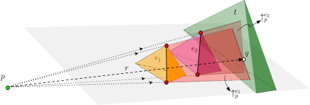
We recall some terminology introduced in [14]. Let $v$ be a vertex of $T$, and let $p$ be a viewpoint. We denote by $\uparrow_{p}^{v}$ the half-line with origin at $p$ in the direction of vector $\overrightarrow{pv}$. Now, let $e=uv$ be an edge of $T$. The vase of $p$ and $e$, denoted $\uparrow_{p}^{e}$, is the region bounded by $e$, $\uparrow_{p}^{u}$, and $\uparrow_{p}^{v}$ (see Fig. 5, right).

Vertices of the viewshed of $p$ can have three types [14]. A vertex of type 1 is a vertex of $T$, of which there are clearly only $n$. A vertex of type 2 is the intersection of an edge of $T$ and a vase. A vertex of type 3 is the intersection of a triangle of $T$ and two vases. With the following two lemmas we will be able to prove Theorem 3.1.

Lemma 1

There are at most $O(n\cdot\pi(T))$ vertices of type $2$.

Proof

Consider an edge $e$ of $T$ and let $H$ be the plane spanned by $e$ and $p$. Consider the viewshed of $p$ on $e$. Let $qr$ be a maximal invisible portion of $e$ surrounded by two visible ones. Since $q$ and $r$ are vertices of type 2, the open segments $pq$ and $pr$ pass through a point of $T$. On the other hand, for any point $x$ in the open segment $qr$, there exist points of $T$ above the segment $px$. This implies that there is a continuous portion of $T$ above $H$ such that the vertical projection onto $H$ of this portion lies on the triangle $pqr$. Such portion has a local maximum in the direction perpendicular to $H$ which is a convex and internal vertex of $T$. In consequence, each invisible portion of $e$ surrounded by two visible ones can be assigned to a distinct point of $T$ that is a local maximum in the direction perpendicular to $H$. Hence, in the viewshed of $p$, $e$ is partitioned into at most $2\pi(T)+3$ parts.

Figure 6: The situation in the proof of Lemma 2.

Lemma 2

There are at most $O(n\cdot\pi(T))$ vertices of type $3$.

Proof

Let $q$ be a vertex of type 3 in the viewshed of $p$. Point $q$ is the intersection between a triangle $t$ of $T$ and two vases, say, $\uparrow_{p}^{e_{1}}$ and $\uparrow_{p}^{e_{2}}$; see Fig. 6. Let $r$ be the ray with origin at $p$ and passing through $q$. Ray $r$ intersects edges $e_{1}$ and $e_{2}$. First, we suppose that $e_{1}$ and $e_{2}$ do not share any vertex and, without loss of generality, we assume that $r\cap e_{1}$ is closer to $p$ than $r\cap e_{2}$. Notice that $r\cap e_{2}$ is a vertex of type 2 because it is the intersection of $e_{2}$ and $\uparrow_{p}^{e_{1}}$, and $\uparrow_{p}^{e_{1}}$ partitions $e_{2}$ into a visible and an invisible portion. Thus, we charge $q$ to $r\cap e_{2}$. If another vertex of type 3 was charged to $r\cap e_{2}$, then such a vertex would also lie on $r$. However, no point on $r$ after $q$ is visible from $p$ because the visibility is blocked by $t$. Hence, no other vertex of type 3 is charged to $r\cap e_{2}$.

If $e_{1}$ and $e_{2}$ are both incident to a vertex $v$, since $t\,\cap\uparrow_{p}^{e_{1}}\cap\uparrow_{p}^{e_{2}}$ is a type 3 vertex, we have that $r$ passes through $v$. Therefore, $q$ is the first intersection point between $r$ (which can be seen as the ray with origin at $p$ and passing through $v$) and the interior of some triangle in $T$. Therefore, any vertex $v$ of $T$ creates at most a unique vertex of type 3 in this way.

Theorem 3.1

The complexity of a viewshed in a 2.5D terrain is $O(n\cdot\pi(T))$.

Next we describe a construction showing that the theorem is best possible.

Theorem 3.2

There exists a 2.5D terrain $T$ with $n$ vertices and prickliness $\pi(T)$, and a viewpoint on $T$ with viewshed complexity $\Theta(n\cdot\pi(T))$.

Proof

Consider the standard quadratic viewshed construction, composed of a set of front mountains and back triangles (Fig. 7 (left)). Notice that there can be at most $\pi(T)$ mountains “at the front”. We add a surrounding box around the construction, see Fig. 7 (right), such that each vertex of the back triangles is connected to at least one vertex on this box. We set the elevation of the box so that it is higher than all the vertices of the back triangles, but lower than those of the front mountains. In this way, no vertex of the back triangles will be a local maximum in any direction, and all local maxima will come from the front.

Figure 7: Schematic top-down view of the classic quadratic construction (left), and the same adapted to have small prickliness (right). The camera with quadratic behaviour is at $(0,-\infty)$ (see Fig. 1 for the resulting view). Blue vertices/edges are low, red are medium hight, and green are high. The right construction introduces a new height (yellow) between medium and high, and changes the triangulation slightly, to ensure that all convex vertices in the construction are green.

4 Prickliness computation in 1.5D TIN terrains

4.1 Algorithm

For every internal and convex vertex $v$ in $T$, we compute $se(v)$ in constant time using the characterization given in Section 2. The prickliness of $T$ is the maximum number of sectors of type $se(v)$ whose intersection is non-empty. We sort the bounding angles of the sectors in $O(n\log n)$ time, and obtain the maximum in a single pass. Thus, we obtain:

Theorem 4.1

The prickliness of a 1.5D terrain can be computed in $O(n\log n)$ time.

4.2 Lower bound

Now we show that $\Omega(n\log n)$ is also a lower bound for finding prickliness in a 1.5D terrain. The reduction is from the problem of checking distinctness of $n$ integer elements, which has an $\Omega(n\log n)$ lower bound in the bounded-degree algebraic decision tree model [17, 29].

Suppose we are given a set ${\cal S}=\{x_{1},x_{2},\ldots,x_{n}\}$ of $n$ integer elements, assumed without loss of generality to be positive. We multiply all elements of $\cal S$ by $180/(\max{\cal S}+1)$ and obtain a new set ${\cal S^{\prime}}=\{x^{\prime}_{1},x^{\prime}_{2},\ldots,x^{\prime}_{n}\}$ such that $0<x^{\prime}_{i}<180$, for each $x^{\prime}_{i}$. We construct a terrain $T$ that will be an instance of the prickliness problem. For each $x^{\prime}_{i}$, we create in $T$ a convex vertex $v_{i}$ such that $se(v_{i})=[x^{\prime}_{i}-\varepsilon,x^{\prime}_{i}+\varepsilon]$, where $\varepsilon=18/(\max{\cal S}+1)$, and such that its two neighbors are at distance $1$ from $v_{i}$. See Fig. 8 for an example. We denote the incident vertices to $v_{i}$ to its left and right by $w^{l}_{i}$ and $w^{r}_{i}$, respectively.

Figure 8: (a) Sectors associated to the element set $\{160,25\}$. (b) The corresponding convex vertices. (c) Construction of the terrain.

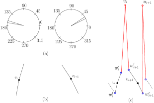
We arrange these convex vertices in the order of the elements in ${\cal S^{\prime}}$ from left to right, and we place all of them at the same height. Then we place a dummy vertex $u_{i}$ between every pair of consecutive vertices $v_{i}$ and $v_{i+1}$, and connect $u_{i}$ to $w^{r}_{i}$ and $w^{l}_{i+1}$; see Fig. 8c. The height of $u_{i}$ is chosen so that its two neighbors become concave vertices, and also so that $[\min{(\cal S^{\prime})}-\varepsilon,\max{(\cal S^{\prime})}+\varepsilon]\subseteq se(u_{i})$. This is possible because moving $u_{i}$ upwards increases its feasible region $se(u_{i})$, the limit being $[0,180]$. The following lemma allows us to prove Theorem 4.2 below.

Lemma 3

The prickliness of $T$ is $n$ if and only if all elements in ${\cal S}$ are distinct.

Proof

Every vertex of type $u_{i}$ satisfies that $[\min{(\cal S^{\prime})}-\varepsilon,\max{(\cal S^{\prime})}+\varepsilon]\subseteq se(u_{i})$. Thus the prickliness of $T$ is at least $n-1$. For every vertex of type $v_{i}$, $se(v_{i})$ has an angle of $2\varepsilon$. Finally, the vertices of type $w^{l}_{i}$ and $w^{r}_{i}$ are concave (or not internal, in the case of $w^{l}_{1}$ and $w^{r}_{n}$) so $se(w^{l}_{i})$ and $se(w^{r}_{i})$ are empty.

Consequently, the prickliness of $T$ is $n$ if and only the sectors of type $se(v_{i})$ are pairwise disjoint, which happens if and only if the elements in ${\cal S}$ are all distinct.

Theorem 4.2

The problem of computing the prickliness of a 1.5D terrain has an $\Omega(n\log n)$ lower bound in the bounded-degree algebraic decision tree model.

5 Prickliness computation in 2.5D terrains

In this section, we consider the problem of computing the prickliness of a 2.5D terrain. In Section 5.1, we present a simple quadratic-time algorithm for TIN terrains. In Section 5.2, we provide evidence that this is close to the best we can do. In Section 5.3, we discuss how to adapt the algorithm for DEM terrains; such an adaptation is needed to be able to run experiments for DEM terrains.

5.1 Algorithm

We propose an algorithm that extends the idea from Section 4.1 to 2.5D terrains as follows: For every convex terrain vertex $v$, we compute the region of the unit sphere $\mathbb{S}^{2}$ containing all vectors $\vec{w}$ such that $v$ is a local maximum of $T$ in direction $\vec{w}$. As we will see, such a region is a cone and we denote it by $co(v)$. Furthermore, we denote the portion of $co(v)$ on the surface of the sphere by $co_{\mathbb{S}^{2}}(v)$.

In order to compute $co(v)$, we consider all edges of $T$ incident to $v$. Let $e=vu$ be such an edge, and consider the plane orthogonal to $e$ through $v$. Let $H$ be the half-space which is bounded by this plane and does not contain $u$. We translate $H$ so that the plane bounding it contains the origin; let $H_{e}$ be the intersection of the obtained half-space with the unit sphere $\mathbb{S}^{2}$. The following property is satisfied: For any unit vector $\vec{w}$ in $H_{e}$, the edge $e$ does not extend further than $v$ in direction $\vec{w}$. We repeat this procedure for all edges incident to $v$, and consider the intersection $co(v)$ of all the obtained half-spheres $H_{e}$. For any unit vector $\vec{w}$ in $co(v)$, none of the edges incident to $v$ extends further than $v$ in direction $\vec{w}$. Since $v$ is convex, this implies that $v$ is a local maxima in direction $\vec{w}$.

Once we know all regions of type $co(v)$, computing the prickliness of $T$ reduces to finding a unit vector that lies in the maximum number of such regions. To simplify, rather than considering these cones on the sphere, we extend them until they intersect the boundary of a unit cube $\mathbb{Q}$ centered at the origin. The conic regions of type $co(v)$ intersect the faces of $\mathbb{Q}$ forming (overlapping) convex regions. Notice that the problem of finding a unit vector that lies in the maximum number of regions of type $co(v)$ on $\mathbb{S}$ is equivalent to the problem of finding a point on the surface of $\mathbb{Q}$ that lies in the maximum number of “extended" regions of type $co(v)$. The second problem can be solved by computing the maximum overlap of convex regions using a topological sweep [7], for each face of the cube.

Computing the intersection between the extended regions of type $co(v)$ (for all convex vertices $v$) and the boundary of $\mathbb{Q}$ takes $O(n\log n)$ time, and topological sweep to find the maximum overlap takes $O(n^{2})$ time. We obtain the following:

Theorem 5.1

The prickliness of a 2.5D terrain can be computed in $O(n^{2})$ time.

5.2 Lower bound

In this section we show that the problem of computing the prickliness of a 2.5D terrain is 3SUM-hard. This implies our result in Theorem 5.1 is likely to be close to optimal: The best-known algorithm for 3SUM runs in $O(n^{2}(\log\log n)^{O(1)}/(\log n)^{2})$ time, and it is believed there are no significantly faster solutions [3].

The reduction is from the following problem, which is known to be 3SUM-hard [12]: Given a square $Q$ and $m$ strips of infinite length, does there exist a point in $Q$ not covered by any of these $m$ strips?

Let us take an instance of the problem above. The complement of each strip is given by two half-planes. Let us consider the $2m$ half-planes obtained in this way, together with the square $Q$. Answering the above question is equivalent to answering whether there exists a point in $Q$ covered by $m$ of the half-planes.

For every half-plane, if it does not intersect $Q$, we discard it. Otherwise, we replace the half-plane by the smallest-area rectangle that contains the intersection of $Q$ with the half-plane; see Fig. 9. Then the problem becomes determining whether there exists a point in $Q$ covered by $m$ of these rectangles.

Figure 9: Instance of the problem of coverage with strips (left), and the equivalent problem of coverage with rectangles (right).

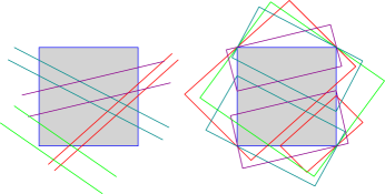
Let $\mathcal{A}$ be the arrangement containing $Q$ and the rectangles. By construction, we have:

Observation 5.2

Any point is covered by at most $m+1$ objects of $\mathcal{A}$. If a point is covered by $m+1$ objects of $\mathcal{A}$, it lies inside $Q$.

Next we consider the plane containing $\mathcal{A}$ as a horizontal plane in $\mathbb{R}^{3}$ such that $(0,0,2)$ lies on $Q$. For every object in $\mathcal{A}$, we connect all its vertices to $(0,0,0)$, which gives a cone, and we intersect this cone with the unit sphere centered at $(0,0,0)$. The intersection of the cone with the surface of the sphere is referred to as the “projection” of the original object in $\mathcal{A}$. We denote the projection of $Q$ by $\tilde{Q}$, and the projection of rectangle $R_{i}$ by $\tilde{R}_{i}$. With some abuse of notation, we still refer to the objects $\tilde{R}_{i}$ as “rectangles”. Let $\tilde{\mathcal{A}}$ be the arrangement containing the projection of the objects in $\mathcal{A}$. Observation 5.2 implies:

Observation 5.3

Any point is covered by at most $m+1$ objects of $\tilde{\mathcal{A}}$. If a point is covered by $m+1$ objects of $\tilde{\mathcal{A}}$, it lies inside $\tilde{Q}$.

We next construct a terrain $T$. The terrain contains red, green and blue vertices. We associate one red vertex to $\tilde{Q}$ and to each of the rectangles intersecting it. The red vertices are placed at height two, and the distance between any pair of them is at least three.

Each red vertex has four green vertices as neighbors, placed as follows. Let $\tilde{R}_{i}$ be one of the rectangles on the sphere (either $\tilde{Q}$ or one of the rectangles intersecting it), and let $v_{i}$ be the red vertex of $T$ associated to $\tilde{R}_{i}$. For each of the sides of $\tilde{R}_{i}$, consider the plane containing the side of $\tilde{R}_{i}$ and passing through the origin. Consider the half-space $H$ that is bounded by this plane and contains $\tilde{R}_{i}$. Take a normal vector $w$ of the plane that does not point towards $H$. Then place a green vertex $x$ of $T$ such that the vector $\vec{v_{i}x}$ is congruent to $w$ and has length one. By following this procedure for all sides of $\tilde{R}_{i}$, we obtain four green vertices of $T$ which are adjacent to $v_{i}$. We denote this set of vertices by $N(v_{i})$. There are no more vertices of $T$ adjacent to $v_{i}$.

Lemma 4

Vertex $v_{i}$ satisfies:

• It is a convex vertex of $T$.

• If we project $v_{i}$ and $N(v_{i})$ onto the $XY$-plane, then the convex hull of the projection of the vertices in $N(v_{i})$ contains the projection of $v_{i}$.

• $co_{\mathbb{S}^{2}}(v_{i})=\tilde{R}_{i}$.

Proof

The intersection of the four half-spaces associated to the four sides of $\tilde{R}_{i}$ forms a cone that can be described as the set of points $\bar{x}\in\mathbb{R}^{3}$ satisfying the equation $A\bar{x}\leq 0$, where $A$ is a $4\times 3$ matrix. It can also be described as $cone(W)$ –the conic hull of vectors in $W$–, where $W$ is the set of four vectors pointing from the origin to the four endpoints of $R_{i}$.

Let $\tilde{W}$ be the $4\times 3$ matrix where each row corresponds to the components of one of the vectors in $W$. Let $\tilde{A}$ be the set of four vectors corresponding to the four rows of $A$. By polar duality, the cones described by $\tilde{W}\bar{x}\leq 0$ and $cone(\tilde{A})$ are also the same.

Notice that the vectors of $\tilde{A}$ are the four vectors used to place the four neighbors of $v_{i}$ in $T$. Therefore, (b) is equivalent to the following: If we project the endpoints of the vectors of $\tilde{A}$ onto the $XY$-plane, then the convex hull of the projected points contains the origin. We will prove that $(0,0,-1)\in cone(\tilde{A})$, which implies this claim.

Since the four endpoints of $\tilde{R}_{i}$ have positive $z$-coordinate, $(0,0,-1)$ satisfies the equation $\tilde{W}\bar{x}\leq 0$. Since the cones $\tilde{W}\bar{x}\leq 0$ and $cone(\tilde{A})$ are the same, we obtain $(0,0,-1)\in cone(\tilde{A})$.

Regarding (a), let $\alpha\neq(0,0,0)$ be such that $A\alpha\leq 0$. Then $cone(\tilde{A})$ is contained in the half-space $\alpha^{T}x\leq 0$, which proves that $v_{i}$ is a convex vertex of $T$.

By construction of $N(v_{i})$ and the fact that $v_{i}$ is a convex vertex of $T$, (c) follows.

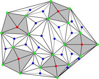
By Lemma 4b (and the facts that red vertices are at pairwise distance at least three and each red vertex has its green neighbors at distance one), the projection of the red and green vertices, and the edges among them, onto the $XY$-plane is a set of pairwise disjoint wheel graphs. Next, we triangulate this graph. Then, for every triangle defined by three green vertices, we place a blue vertex inside the triangle and we connect this vertex to the three vertices of the triangle (see Fig. 10). It only remains to specify the height of the blue vertices. Each blue vertex $u$ is placed at a height high enough so that: (i) the three neighboring green vertices become non-convex vertices of $T$, and (ii) $co_{\mathbb{S}^{2}}(u)$ contains $\tilde{Q}$. Regarding (ii), if $u$ is placed higher than all of its neighbors (which are all green, so they already have specified heights), then $co_{\mathbb{S}^{2}}(u)$ contains the north pole. By moving $u$ upwards, $co(u)$ becomes bigger and bigger, the limit being the upper hemisphere of $\mathbb{S}$. Therefore, from some height onwards $co_{\mathbb{S}^{2}}(u)$ contains $\tilde{Q}$. Let $\tilde{\mathcal{A}}^{+}$ be the arrangement $\tilde{\mathcal{A}}$ augmented with $co_{\mathbb{S}^{2}}(u)$ for all blue vertices $u$. Let the number of blue vertices be $k$. By Observation 5.3,

Figure 10: Projection of $T$ onto the $XY$-plane.

Observation 5.4

Any point is covered by at most $m+1+k$ objects of $\tilde{\mathcal{A}}^{+}$. If a point is covered by $m+1+k$ objects of $\tilde{\mathcal{A}}^{+}$, it lies inside $\tilde{Q}$.

Lemma 5

The prickliness of $T$ is $m+k+1$ if and only if there is a point in $Q$ covered by $m$ rectangles.

Proof

Suppose that the prickliness of $T$ is $m+k+1$. This means that, when we compute $co(v)$ for all vertices $v$ of $T$, a unit vector that is covered by the maximum number of such cones is covered by $m+k+1$ cones. If $v$ is a blue vertex, $co_{\mathbb{S}^{2}}(v)$ contains $\tilde{Q}$. If $v$ is a green vertex, $co(v)$ is empty because $v$ is a concave vertex of $T$. If $v$ is a red vertex, either $v$ is associated to $\tilde{Q}$ or $v=v_{i}$ for some $i$. By Lemma 4c, in the first case $co_{\mathbb{S}^{2}}(v)=\tilde{Q}$, while in the second case $co_{\mathbb{S}^{2}}(v)=\tilde{R_{i}}$. Therefore, the problem of computing the prickliness of $T$ is equivalent to the problem of finding a point in $\tilde{\mathcal{A}}^{+}$ covered by the maximum number of objects. By Observation 5.3, if the prickliness of $T$ is $m+k+1$, there is a point in $\tilde{Q}$ covered by $m+1+k$ objects of $\tilde{\mathcal{A}}^{+}$. This implies that there is a point in $Q$ covered by $m$ rectangles.

If there is a point in $Q$ covered by $m$ rectangles, there is a point in $\tilde{Q}$ covered by $m+1+k$ objects of $\tilde{\mathcal{A}}^{+}$. By Observation 5.3, there is no point in $\tilde{\mathcal{A}}^{+}$ covered by more than $m+1+k$ objects, so the prickliness of $T$ is $m+k+1$.

Thus we have the following:

Theorem 5.5

The problem of computing the prickliness of a 2.5D terrain is 3SUM-hard.

5.3 Algorithm for DEMs

The prickliness of a DEM terrain can be computed using the same algorithm as for TINs: Each cell center can be seen as a vertex $v$, and its neighbors are the cell centers of its eight neighboring cells. The edges connecting $v$ to its neighbors can then be used to compute $co(v)$ as in Section 5.1, and the rest of the algorithm follows. However, DEM terrains have significantly more vertices, and vertices have on average more neighbors; this causes a significant increase in computation time and, more importantly, in memory usage. For this reason, in our experiments, the prickliness values for the DEM terrains were approximated.

The approximated algorithm discretizes the set of vectors that are candidates to achieve prickliness as follows: For every interior cell $g$ of the terrain, we translate a horizontal grid $G$ of size $n$ by $n$ and cell size $s$ above the cell center $v$ of $g$ in a way that $v$ and the center of $G$ are vertically aligned and at distance one. Then the vectors considered as potential prickliness are those with origin at $v$ and endpoint at some cell center $c$ in $G$. For any such vector lying inside $co(v)$, the value of $c$ gets incremented by one. When all interior cells of the terrain have been processed, a cell center of $G$ with maximum value gives the approximated prickliness of the terrain. Cell size $s$ was set to $0.05$, based on the spread of the results on TIN terrains. This method should, in practice, produce a close approximation of prickliness.

This algorithm is the last contribution of the theoretical block of this paper. We next move to the experimental block.

Part II Experiments

6 Existing topographic attributes

Since one of the goals of our experiments is to verify our hypothesis that existing topographic attributes do not provide a good indicator of the viewshed complexity, in our experiments we consider the following topographic attributes (in addition to prickliness).

Terrain Ruggedness Index (TRI)

The Terrain Ruggedness Index measures the variability in the elevation of the terrain [24]. Riley et al. originally defined TRI specifically for DEM terrains as follows. Let $c$ be a cell of the terrain, and let $\mathcal{N}(c)$ denote the set of (at most) eight neighboring cells of $c$. The TRI of $c$ is then defined as

$$\mathit{pTRI}(c)=\sqrt{\frac{1}{\lvert\mathcal{N}(c)\rvert}\sum_{q\in\mathcal{N}(c)}\left(c_{z}-q_{z}\right)^{2}},$$

where $\lvert\mathcal{N}(c)\rvert$ denotes the cardinality of $\mathcal{N}(c)$. Hence, $\mathit{pTRI}(c)$ essentially measures the standard deviation of the difference in height between $c$ and the points in $\mathcal{N}(c)$. The Terrain Roughness Index $\mathit{TRI}(T)$ of $T$ is the average $\mathit{pTRI}(T,c)$ value over all cells $c$ in $T$.

For TINs, we have adapted the definition as follows: $\mathcal{N}(c)$ is defined as the set of vertices which are adjacent to a given vertex $c$ in $T$. The Terrain Roughness Index $\mathit{TRI}(T)$ is then obtained as the average $\mathit{pTRI}(T,c)$ value over all vertices $c$ of $T$.

Terrain Shape Index (TSI)

The Terrain Shape Index also measures the “shape” of the terrain [20]. Let $\mathcal{C}(c,r,T)$ denote the intersection of $T$ with a vertical cylinder of radius $r$ centered at $c$ (so after projecting all points to the plane, the points in $\mathcal{C}(c,r,T)$ lie on a circle of radius $r$ centered at $c$). For ease of computation, we discretize $\mathcal{C}(c,r,T)$: for DEMs we define $C(c,r,T)$ to be the grid cells intersected by $\mathcal{C}(c,r,T)$, and for TINs we define $C(c,r,T)$ as a set of 360 equally spaced points on $\mathcal{C}(c,r,T)$. The TSI of a point $c$ is then defined as

$$\mathit{pTSI}(c,r,T)=\frac{1}{r\lvert C(c,r,T)\rvert}\sum_{q\in C(c,r,T)}c_{z}-q_{z}\ ,$$

and essentially measures the average difference in height between “center” point $c$ and the points at (planar) distance $r$ to $c$, normalized by $r$. The Terrain Shape Index $\mathit{TSI}(T,r)$ of the entire terrain $T$ is the average $\mathit{pTSI}(c,r,T)$ over all cells (in case of a DEM) or vertices (in case of a TIN) of $T$. We choose $r=1000$m (which is roughly eight percent of the width of our terrains) in our experiments.

Fractal dimension (FD)

The (local) fractal dimension measures the roughness around a point $c$ on the terrain over various scales [18, 26]. We use the definition of Taud and Parrot [26] that uses a box-counting method, and is defined as follows. Let $w$ be the width of a cell in the DEM, and let $s\in\mathbb{N}$ be a size parameter. For $q\in 1..s/2$, consider subdividing the cube with side length $sw$ centered at $c$ into $(s/q)^{3}$ cubes of side length $qw$. Let $\mathcal{C}_{s}(c,q)$ denote the resulting set of cubes, and define $N_{s}(c,q,T)$ as the number of cubes from $\mathcal{C}_{s}(c,q)$ that contain a “unit” cube from $\mathcal{C}_{s}(c,1)$ lying fully below the terrain $T$. Let $\ell_{s}(c,T)$ be the linear function that best fits (i.e. minimizes the sum of squared errors) the set of points $\{(\ln(q),\ln(N_{s}(c,q,T)))\mid q\in 1..s/2\}$ resulting from those measurements. The fractal dimension $\mathit{pFD}_{s}(c,T)$ at $c$ is then defined as the inverse of the slope of $\ell_{s}(c,T)$. The fractal dimension $\mathit{FD}(T,s)$ of the DEM terrain itself is again the average over all DEM cells. Following Taud and Parrot we use $s=24$ in our experiments. For our TIN terrains, we keep $w$ the same as in their original DEM representations, and average over all vertices.

7 Experiments

In this section we present our experimental setup. Our goals are to

• verify our hypothesis that existing topographic attributes do not provide a good indicator of the viewshed complexity,

• evaluate whether prickliness does provide a good indicator of viewshed complexity in practice, and

• evaluate whether these results are consistent for DEMs and TINs.

Furthermore, since in many applications we care about the visibility of multiple viewpoints (e.g. placing guards or watchtowers), we also investigate these questions with respect to the complexity of the common viewshed of a set of viewpoints. In this setting a point is part of the (common) viewshed if and only if it can be seen by at least one viewpoint. Note that since Theorem 3.1 proves that the complexity of a viewshed is proportional to the prickliness, our second goal is mainly to evaluate the practicality of prickliness. That is, to establish if this relation is also observable in practice or that the hidden constants in the big-O notation are sufficiently large that the relation is visible only for very large terrains.

Next, we briefly describe our implementations of the topographic attributes. We then outline some basic information about the terrain data that we use as input, and we describe how we select the viewpoints for which we compute the viewsheds.

Implementations

We consider prickliness and the topographic attributes from Section 6. To compute the prickliness we implemented the algorithm from Theorem 5.1 in C++ using CGAL 5.0.2 [27] and its 2D arrangements [28] library. We also implemented the algorithms for TRI, TSI, and FD on TINs. These are mostly straightforward. To compute the viewsheds on TINs we implemented the hidden-surface elimination algorithm of [13] using CGAL. We remark that our implementation computes the exact TIN viewsheds, as opposed to previous studies that only considered fully visible triangles (e.g., [23]).

To compute the prickliness on DEMs we used the algorithm from Section 5.3. For TRI, TSI, and FD on DEMs we used the implementations available in ArcGIS Pro 2.5.1 [9]. To compute viewsheds on DEMs we used the builtin tool “Viewshed 2” in ArcGIS with a vertical offset of 1 meter, which produces a raster with boolean values that indicate if a cell is visible or not. To get a measure of complexity similar to that of the TINs we use the “Raster to Polygon” functionality of ArcGIS (with its default settings) to convert the set of True cells into a set of planar polygons (possibly with holes). We use the total number of vertices of these polygons as the complexity of the viewshed on a DEM.

Terrains

We considered a collection of 52 real-world terrains around the world. These terrains were handpicked in order to cover a large variety of landscapes, with varying ruggedness, including mountainous regions (Rocky mountains, Himalaya), flat areas (farmlands in the Netherlands), and rolling hills (Sahara), and different complexity. We obtained the terrains from the United States Geological Survey (USGS), and converted them through the Terrain world elevation layer [10] in ArcGIS [9]; all terrains use the WGS 1984 Web Mercator (auxiliary sphere) map projection. Each terrain is represented as a 10-meter resolution DEM of size 1400$\times$1200. According to past studies the chosen resolution of 10 meters provides the best compromise between high resolution and processing time of measurements [19, 30]. The complete list of terrains with their extents can be found in [21].

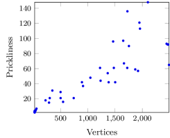
We generated a TIN terrain for each DEM using the “Raster to TIN” function in ArcGIS [9]. This function generates a Delaunay triangulation to avoid long, thin triangles as much as possible. With the $z$-tolerance setting, the triangulation complexity can be controlled by determining an allowed deviation from the DEM elevation values. We considered TIN terrains generated using a $z$-tolerance of 50 meters. This resulted in TINs where the number of vertices varied between 30 and 5808 (with an average of 1547 vertices). Their distribution can be seen in Fig. 12.

Viewpoints

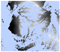
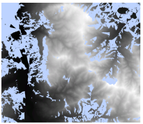
Kim et al. [16] found that placing the viewpoints at peaks typically produces viewsheds that cover hilltops, but not many valleys, whereas placing viewpoints in pits typically covers valleys but not hilltops. This leads us to consider three different strategies to pick the locations of the viewpoints: picking “high” points (to cover peaks), picking “low” points (to cover valleys), and picking viewpoints uniformly at random. To avoid clusters of high or low viewpoints we overlay an evenly spaced grid on the terrain, and pick one viewpoint from every grid cell (either the highest, lowest, or a random one). We pick these points based on the DEM representation of the terrains, and place the actual viewpoints one meter above the terrain to avoid degeneracies. We use the same locations in the TINs in order to compare the results between TINs and DEMs (we do recompute the $z$-coordinates of these points so that they remain 1m above the surface of the TIN). The resulting viewsheds follow the expected pattern; refer to Fig. 11. In our experiments, we consider both the complexity of a viewshed of a single viewpoint as well as the combined complexity of a viewshed of nine viewpoints (picked from a $3\times 3$ overlay grid). Results of Kammer et al. [15] suggest that for the size of terrains considered these viewpoints already cover a significant portion of the terrain, and hence picking even more viewpoints is not likely to be informative.

Figure 11: (left) A joint viewshed (blue) created from viewpoints placed on the highest points. (right) A joint viewshed (blue) created from viewpoints placed on the lowest points.

Analysis

For each topographic attribute we consider its value in relation to the complexity of the viewsheds. In addition, we test if there is a correlation between the viewshed complexity and the attribute in question. We compute their sample correlation coefficient (Pearson correlation coefficient) $R$ to measure their (linear) correlation. The resulting value is in the interval $[-1,1]$, where a value of $1$ implies that a linear increase in the attribute value corresponds to a linear increase in the viewshed complexity. A value of $-1$ would indicate that a linear increase in the attribute leads to a linear decrease in viewshed complexity, and values close to zero indicate that there is no linear correlation.

8 Results

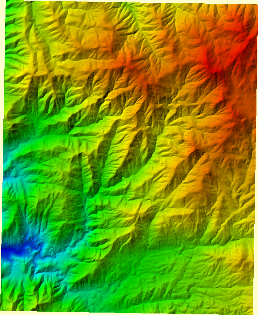
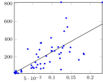
We start by investigating the prickliness values compared to the complexity of the terrains considered. These results are shown in Fig. 12. We can see that the prickliness is generally much smaller than the number of vertices in the (TIN representation of the) terrain. In Fig. 13 we also see the $\pi_{\vec{v}}$ values for orientation vectors near $(0,0,1)$ (recall that the maximum over all orientations defines the prickliness).

Figure 12: The prickliness values for the terrains we considered.

Figure 13: (left) A real-world terrain with $583$ vertices from the neighborhood of California Hot Springs whose prickliness is only $62$. (right) The value $\pi_{\vec{v}}$ for vectors near $(0,0,1)$.

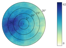
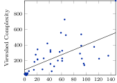
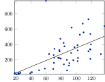
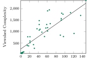
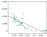
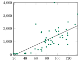
Next, we analyze the relation between topographic attributes and viewshed complexity. For each of the terrains we compute the viewshed of one or nine viewpoints, for three viewpoint placement strategies, and analyze the complexity of the viewshed as a function of the topographic attributes both for TINs and DEMs. Table 1 summarizes the correlation between the attributes and the viewshed complexity for each case.

	TIN						DEM
	highest		lowest		random		highest		lowest		random
	single	multi	single	multi	single	multi	single	multi	single	multi	single	multi
Prick	0.75	0.97	0.41	0.83	0.64	0.93	0.63	0.90	0.10	0.19	0.18	0.64
TRI	0.44	0.58	0.62	0.72	0.61	0.63	-0.52	-0.38	-0.27	-0.30	-0.34	-0.43
TSI	0.45	0.69	0.69	0.81	0.63	0.75	-0.53	-0.40	-0.24	-0.23	-0.32	-0.42
FD	-0.56	-0.73	-0.64	-0.78	-0.66	-0.76	0.11	-0.27	0.27	0.25	0.27	-0.01

Table 1: The correlation coefficients ($R$ values) between the attributes and viewshed complexity.

TIN results

In this case we distinguish between single and multiple viewpoints.

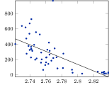
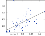
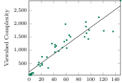
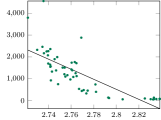
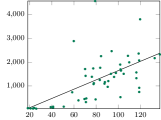
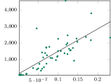
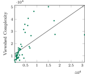
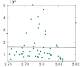
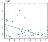
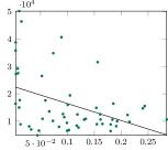
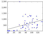
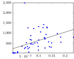
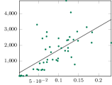
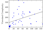
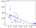
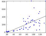
For single viewpoints, the first row in Fig. 14 shows the full results for a randomly placed viewpoint on the TIN. Somewhat surprisingly, we see that terrains with high fractal dimension have a low viewshed complexity. For the other measures, higher values tend to correspond to higher viewshed complexities. However, the scatter plots for TRI and TSI show a large variation. The scatter plots for the other placement strategies (highest and lowest) look somewhat similar (see Fig. 17 and 18 in Appendix 0.A), hence the strategy with which we select the viewpoints does not seem to have much influence in this case. None of the four attributes shows a strong correlation in this case (see also Table 1). Prickliness shows weak-medium correlation in three out of six cases, strong correlation for one case—viewpoints at highest points—and no correlation for two cases with viewpoints at lowest points. The other attributes show an even weaker correlation in general.

Prickliness	FD	TRI	TSI

Figure 14: The viewshed complexity on a TIN. First row: single random viewpoint. Second row: common viewshed of multiple (nine, selected from a $3\times 3$ overlay) random viewpoints.

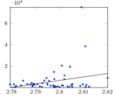
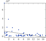
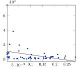
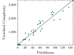
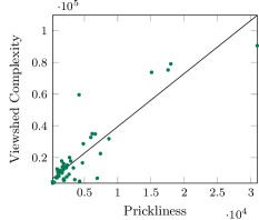
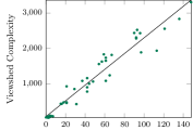
For multiple viewpoints, selected from a $3\times 3$ overlay grid (refer to Section 7), the results are presented in the second row of Fig. 14. Again, fractal dimension shows an inverse behavior. In contrast, the other three attributes show now a much clearer positive correlation with viewshed complexity. In this case the prickliness shows the strongest correlation in all but one case (that of viewpoints at lowest points). In particular when placing the viewpoints at highest points within the overlay grids the correlation is strong. See also Fig. 16 (left).

Prickliness	FD	TRI	TSI

Figure 15: The viewshed complexity on a DEM. First row: single random viewpoint. Second row: common viewshed of multiple (nine, selected from a $3\times 3$ overlay) random viewpoints.

TIN	DEM

Figure 16: The complexity of the common viewshed of nine viewpoints placed using the highest strategy on a TIN (left) or on a DEM (right).

DEM results

In this case, the results for placing a single viewpoint and placing the viewpoints in a $3\times 3$ grid appear somewhat similar. Since the results for the $3\times 3$ grid are more pronounced, we focus on those results.

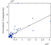
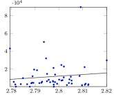
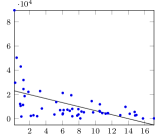
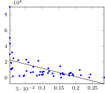
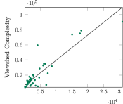
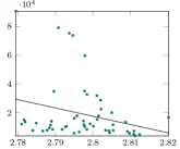
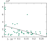
For viewpoints placed randomly, the first row of plots in Fig. 15 corresponds to the complexity of a single viewshed, whereas the second row corresponds to the complexity of the common viewshed of nine viewpoints selected from a $3\times 3$ overlay. The correlation values obtained in this setting are shown in the two rightmost columns of Table 1. In contrast to TINs, for DEMs all measures show no to weak correlation values, even though prickliness obtains the highest correlation coefficient in the case of multiple viewpoints (0.64).

For viewpoints placed at lowest points the correlation values are very low, both for single and multiple viewpoints (the scatter plots are shown in Fig. 20 in Appendix 0.A).

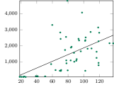
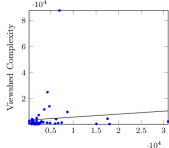
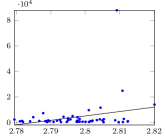
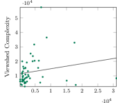
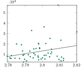
In the case of viewpoints placed at highest points, correlation results are still weak for all measures except for prickliness (see the scatter plots in Fig. 19 in Appendix 0.A). Here prickliness shows a moderate correlation for single viewpoints, but a very high correlation for multiple viewpoints (coefficient 0.90). However, the scatter plot (Fig. 16 right), where most of the plot points lie in a small region of the plot, suggests that this value may not be very meaningful.

Finally, it should also be noted that prickliness is not the only attribute that has very different behavior between TINs and DEMs; indeed, the other three attributes also show a very large variation between these two types of terrain models.

9 Discussion

The experimental results for TINs confirm our hypotheses. We can see a clear correlation between the viewshed complexity and the prickliness, especially when multiple viewpoints are placed on the highest points. In contrast, this is not evident for the other three topographic attributes considered. The terrain ruggedness index (TRI) and terrain shape index (TSI) show some very weak positive correlation, but not as strong as prickliness. This could be explained by the fact that TRI and TSI only consider a fixed neighborhood around each point, making them local measures unable to capture the whole viewshed complexity. Indeed, a small (local) obstruction can be enough to significantly alter the value for any of these attributes. The fractal dimension (FD) seems to be even worse at predicting viewshed complexity. Unlike TRI and TSI, this topographic attribute considers the variability within an area of the terrain as opposed to a fixed-radius neighborhood. Taking a closer look at the FD values for both terrain datasets shows a minimal variation, with most of them being close to 3.0, which, according to Taud et al. [26], indicates a nearly-constant terrain. These results seem to indicate that this measure fails to detect the variation in elevation levels with the chosen parameters.

The situation for DEM terrains is less clear. Only for viewsheds originating from the highest points we see a strong correlation between prickliness and viewshed complexity. When the viewpoints are placed at the lowest points of the DEM terrains, the correlation disappears. Since the prickliness measures the amount of peaks in the terrain in all possible (positive) directions, this means that when a viewpoint is placed at the highest elevation and the viewshed gets split up by the protrusions (which seem to be accurately tracked by prickliness), there is a strong correlation. However, when the viewpoints are placed at the lowest points, the viewsheds become severely limited by the topography of the terrain surrounding them. Even when placing multiple viewpoints, these viewsheds do not seem to encounter enough of the protrusions that are detected by the prickliness measure for viewpoints placed at high points.

One possible explanation for the difference between the results on the TIN and DEM terrains for prickliness could be attributed to the difference in resolution between the DEMs and TINs used. The DEMs used consisted of 1.68M cells of 10m size, while the TINs—generated with an error tolerance of 50m—had 1547 vertices on average. While it would have been interesting to use a higher resolution TIN, this was not possible due to the high memory usage of the prickliness algorithm. Another possible explanation for the mismatch between the results for TINs and DEMs may be on the actual definition of prickliness, which is more natural for TINs than for DEMs. Indeed, it can be seen in the results that the prickliness values for DEMs are much higher than for TINs, which could indicate that the definition is too sensitive to small terrain irregularities.

10 Conclusion

We established that prickliness is a reasonable measure of potentially high viewshed complexity, at least for TINs, confirming our theoretical results. Moreover, prickliness shows a much clearer correlation with viewshed complexity than the three other terrain attributes considered.

One aspect worth further investigation is its correlation for DEMs, which seems to be much weaker. One explanation for this might be that the definition of prickliness is more natural for TINs than for DEMs, but there are several other possible explanations, and it would be interesting future work to delve further into this phenomenon. Having established that prickliness can be a useful terrain attribute, it remains to improve its computation time, so it can be applied to larger terrains in practice.

Finally, during our work we noticed that several of the terrain attributes are defined locally, and are parameterized by some neighborhood size. Following previous work, we aggregated these local measures into a global measure by averaging the measurements. It may be worthwhile to investigate different aggregation methods as well. This also leads to a more general open question on how to “best” transform a local terrain measurement into a global one.

Acknowledgments

The authors would like to thank Jeff Phillips for a stimulating discussion that, years later, led to the notion of prickliness. They would also like to thank Ramesh K. Jallu for his work on previous versions of this paper, and Hans Raj Tiwary for key observations in Sections 5.1 and 5.2.

A.A. and M.S. were supported by the Czech Science Foundation, grant number GJ19-06792Y. M.L. was partially supported by the Netherlands Organization for Scientific Research (NWO) under project no. 614.001.504. R.S. was supported by project PID2019-104129GB-I00/ MCIN/ AEI/ 10.13039/501100011033. This project has received funding from the European Union’s Horizon 2020 research and innovation programme under the Marie Skłodowska-Curie grant agreement No 734922. The work was (partially) done while A.A. and M.S. were affiliated with Institute of Computer Science of the Czech Academy of Sciences, with institutional support RVO:67985807.

Appendix 0.A Additional plots

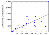
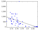
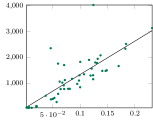
In this section, we provide the scatter plots for the placement strategies of choosing “high” points and for choosing “low” points. Plots for TINs are displayed in Fig. 17 and 18, while plots for DEMs are shown in Fig. 19 and 20.

Prickliness	FD	TRI	TSI

Figure 17: The viewshed complexity on a TIN. First row: single highest viewpoint. Second row: common viewshed of multiple (nine, selected from a $3\times 3$ overlay) highest viewpoints.

Prickliness	FD	TRI	TSI

Figure 18: The viewshed complexity on a TIN. First row: single lowest viewpoint. Second row: common viewshed of multiple (nine, selected from a $3\times 3$ overlay) lowest viewpoints.

Prickliness	FD	TRI	TSI

Figure 19: The viewshed complexity on a DEM. First row: single highest viewpoint. Second row: common viewshed of multiple (nine, selected from a $3\times 3$ overlay) highest viewpoints.

Prickliness	FD	TRI	TSI

Figure 20: The viewshed complexity on a DEM. First row: single lowest viewpoint. Second row: common viewshed of multiple (nine, selected from a $3\times 3$ overlay) lowest viewpoints.

References

- [1] de Berg, M., Haverkort, H.J., Tsirogiannis, C.P.: Visibility maps of realistic terrains have linear smoothed complexity. J. Comput. Geom. 1(1), 57–71 (2010)
- [2] Chamberlain, B.C., Meitner, M.J.: A route-based visibility analysis for landscape management. Landscape and Urban Planning 111, 13–24 (2013)
- [3] Chan, T.M.: More logarithmic-factor speedups for 3SUM, (median, +)-convolution, and some geometric 3SUM-hard problems. ACM Trans. Algorithms 16(1), 7:1–7:23 (2020)
- [4] Danese, M., Nolè, G., Murgante, B.: Identifying viewshed: New approaches to visual impact assessment. In: Geocomputation, Sustainability and Environmental Planning, pp. 73–89. Springer, Berlin, Heidelberg (2011)
- [5] Dean, D.J.: Improving the accuracy of forest viewsheds using triangulated networks and the visual permeability method. Canadian Journal of Forest Research 27(7), 969–977 (1997)
- [6] Dong, Y., Tang, G., Zhang, T.: a Systematic Classification Research of Topographic Descriptive Attribute in Digital Terrain Analysis. The International Archives of the Photogrammetry, Remote Sensing and Spatial Information Sciences 37 B2, 357–362 (2008)
- [7] Edelsbrunner, H., Guibas, L.J.: Topologically sweeping an arrangement. Journal of Computer and System Sciences 38(1), 165–194 (1989)
- [8] Environmental Systems Research Institute (ESRI): How Geodesic Viewshed works. https://pro.arcgis.com/en/pro-app/latest/tool-reference/3d-analyst/how-viewshed-2-works.htm, accessed: 2022-10-17
- [9] Environmental Systems Research Institute (ESRI): Arcgis pro (2.5.1) (05 2020)
- [10] Environmental Systems Research Institute (ESRI): Terrain, scale: 10m (02 2020)
- [11] Franklin, W.R., Vogt, C.: Multiple observer siting on terrain with intervisibility or lo-res data. In: XXth Congress, International Society for Photogrammetry and Remote Sensing. pp. 12–23 (2004)
- [12] Gajentaan, A., Overmars, M.H.: On a class of O() problems in computational geometry. Comput. Geom. 5(3), 165–185 (1995)
- [13] Goodrich, M.T.: A polygonal approach to hidden-line and hidden-surface elimination. CVGIP: Graphical Models and Image Processing 54(1), 1–12 (jan 1992)
- [14] Hurtado, F., Löffler, M., Matos, I., Sacristán, V., Saumell, M., Silveira, R.I., Staals, F.: Terrain visibility with multiple viewpoints. International Journal of Computational Geometry & Applications 24(04), 275–306 (2014)
- [15] Kammer, F., Löffler, M., Mutser, P., Staals, F.: Practical approaches to partially guarding a polyhedral terrain. In: Proc. 8th International Conference on Geographic Information Science. pp. 318–332. LNCS 8728 (2014)
- [16] Kim, Y.H., Rana, S., Wise, S.: Exploring multiple viewshed analysis using terrain features and optimisation techniques. Computers & Geosciences 30(9), 1019–1032 (2004)
- [17] Lubiw, A., Rácz, A.: A lower bound for the integer element distinctness problem. Inf. Comput. 94(1), 83–92 (1991)
- [18] Mandelbrot, B.B.: The fractal geometry of nature. W.H. Freeman, New York (1982)
- [19] Maynard, J.J., Johnson, M.G.: Scale-dependency of LiDAR derived terrain attributes in quantitative soil-landscape modeling: Effects of grid resolution vs. neighborhood extent. Geoderma 230-231, 29–40 (2014)
- [20] McNab, W.H.: Terrain shape index: Quantifying effect of minor landforms on tree height. Forest Science 35, 91–104 (1989)
- [21] Meijer, G.: Realistic terrain features and the complexity of joint viewsheds. Master’s thesis, Utrecht University (2020)
- [22] Moet, E., van Kreveld, M., van der Stappen, A.F.: On realistic terrains. Computational Geometry 41(1), 48–67 (2008)
- [23] Riggs, P.D., Dean, D.J.: An investigation into the causes of errors and inconsistencies in predicted viewsheds. Transactions in GIS 11(2), 175–196 (2007)
- [24] Riley, S.J., DeGloria, S.D., Elliot, R.: A terrain ruggedness index that quantifies topographic heterogeneity. Journal of Science 5, 23–27 (1999)
- [25] Schirpke, U., Tasser, E., Tappeiner, U.: Predicting scenic beauty of mountain regions. Landscape Urban Plan. 111, 1–12 (2013)
- [26] Taud, H., Parrot, J.F.: Measurement of DEM roughness using the local fractal dimension. Géomorphologie : relief, processus, environnement 11(4), 327–338 (2005)
- [27] The CGAL Project: CGAL User and Reference Manual. CGAL Editorial Board, , 5.0.2 edn. (2020)
- [28] Wein, R., Berberich, E., Fogel, E., Halperin, D., Hemmer, M., Salzman, O., Zukerman, B.: 2d arrangements. In: CGAL User and Reference Manual. CGAL Editorial Board, , 5.0.2 edn. (2020)
- [29] Yao, A.C.: Lower bounds for algebraic computation trees with integer inputs. SIAM J. Comput. 20(4), 655–668 (1991)
- [30] Zhang, W., Montgomery, D.R.: Digital elevation model grid size, landscape representation, and hydrologic simulations. Water Resources Research 30(4), 1019–1028 (1994)