Real-Time Surface Fitting to RGBD Sensor Data

Abstract

This article describes novel approaches to quickly estimate planar surfaces from RGBD sensor data. The approach manipulates the standard algebraic fitting equations into a form that allows many of the needed regression variables to be computed directly from the camera calibration information. As such, much of the computational burden required by a standard algebraic surface fit can be pre-computed. This provides a significant time and resource savings, especially when many surface fits are being performed which is often the case when RGBD point-cloud data is being analyzed for normal estimation, curvature estimation, polygonization or 3D segmentation applications. Using an integral image implementation, the proposed approaches show a significant increase in performance compared to the standard algebraic fitting approaches.

Real-time perception of scene geometry is an important problem to the machine vision and robotics community. Solutions to this problem play a crucial role in software systems that seek to endow machines with a structural understanding of their environment. Applications of these algorithms include scene navigation, interaction, and comprehension.

Recently developed RGBD sensors have become popular for measuring both scene appearance and geometry. These sensors provide high resolution visual data in a low cost (~$200USD) and compact package. RGBD sensors combine a traditional color camera (RGB) with an infrared depth sensor (D), and merge this data to produce HD color+range images at real-time frame rates (~30 fps). Unlike traditional 2D cameras, RGBD sensors provide depth measurements that directly impart a sense of scene geometry, without the use of techniques such as stereoscopic reconstruction. These sensors have seen increased use as research tools for many computer vision related problems [1].

The volume of data produced by such sensors is quite large. As such, real-time systems must carefully consider the computational cost of algorithms that process this data. This is particularly important for time sensitive tasks such as visual odometry-based navigation, which relies on incoming sensor data to navigate geometrically complex scenes.

For those RGBD algorithms that analyze the depth image, it is common to extract geometric surfaces, e.g., planes and quadric surfaces, from the sensed depth images. Fit surfaces often provide important clues for both odometry, e.g., how the robot has moved, and for navigation, i.e., identifying navigable regions of the scene. This article focuses on planar surface fitting to point cloud data, a common task for geometric scene analysis and segmentation algorithms such as surface normal and curvature estimation, polygonization, and 3D segmentation [2].

This work describes a computationally efficient method for fitting planar surfaces to RGBD data, suitable for real-time operation. This formulation improves upon existing approaches by separating the traditional least squares fitting problem into components including the intrinsic camera parameters- which can be precomputed, and quantities related to the disparity of the incoming depth data. When implemented using integral images, this approach results in increased performance when compared to the traditional formulation of these plane fitting methods.

I Prior Work & Background Information

It is necessary to discuss several results from prior work to provide context for the contribution of this article and to lay preliminary groundwork for the technical approach of the proposed algorithm. This section includes a discussion of how $(X,Y,Z)$ point clouds are computed from RGBD sensor data, the nature of RGBD sensor data noise, and a discussion of leading approaches for 3D planar surface estimation from point cloud data.

I-A Point Cloud Reconstruction

Measured 3D $(X,Y,Z)$ positions of sensed surfaces can be directly computed from the intrinsic RGBD camera parameters and the measured depth image values. The $Z$ coordinate is directly taken as the depth value and the $(X,Y)$ coordinates are computed using the pinhole camera model. In a typical pinhole camera model, 3D $(X,Y,Z)$ points are projected to $(x,y)$ image locations, e.g., for the image columns the $x$ image coordinate is $x=f_{x}\frac{X}{Z}+c_{x}-\delta_{x}$. However, for a depth image, this equation is re-organized to “back-project” the depth into the 3D scene and recover the 3D $(X,Y)$ coordinates as shown by equation (1)

$$\begin{array}[]{ccc}X&=&(x+\delta_{x}-c_{x})Z/f_{x}\\ Y&=&(y+\delta_{y}-c_{y})Z/f_{y}\\ Z&=&Z\end{array}$$ (1)

where $Z$ denotes the sensed depth at image position $(x,y)$, $(f_{x},f_{y})$ denotes the camera focal length (in pixels), $(c_{x},c_{x})$ denotes the pixel coordinate of the image center, i.e., the principal point, and $(\delta_{x},\delta_{y})$ denote adjustments of the projected pixel coordinate to correct for camera lens distortion.

I-B Measurement Noise

Studies of accuracy for the Microsoft Kinect sensor show that a Gaussian noise model provides a good fit to observed measurement errors on planar targets where the distribution parameters are mean $0$ and standard deviation $\sigma_{Z}=\frac{m}{2f_{x}b}Z^{2}$ for depth measurements where $\frac{m}{f_{x}b}=-2.85e^{-3}$ is the linearized slope for the normalized disparity empirically found in [3]. Since 3D the coordinates for $(X,Y)$ are a function of both the pixel location and the depth, their distributions are also known as shown below:

$$\begin{array}[]{ccc}\sigma_{X}&=&\frac{x-c_{x}+\delta_{x}}{f_{x}}\sigma_{Z}=\frac{x-c_{x}+\delta_{x}}{f_{x}}(1.425e^{-3})Z^{2}\\ \sigma_{Y}&=&\frac{y-c_{y}+\delta_{y}}{f_{y}}\sigma_{Z}=\frac{y-c_{y}+\delta_{y}}{f_{y}}(1.425e^{-3})Z^{2}\\ \sigma_{Z}&=&\frac{m}{f_{x}b}Z^{2}\sigma_{d^{\prime}}=(1.425e^{-3})Z^{2}\end{array}$$ (2)

These equations indicate that 3D coordinate measurement uncertainty increases as a quadratic function of the depth for all three coordinate values. However, the quadratic coefficient for the $(X,Y)$ coordinate standard deviation is at most half that in the depth direction, i.e., $(\sigma_{X},\sigma_{Y})\approx 0.5\sigma_{Z}$ at the image periphery where $\frac{x-c_{x}}{f}\approx 0.5$, and this value is significantly smaller for pixels close to the optical axis.

I-C Implicit Plane Fitting to Point Cloud Data

This section discussed the typical approach for 3D plane fitting which estimated the plane when expressed as an implicit polynomial. We refer to this approach as the implicit fitting method which seeks to minimize the square of the perpendicular distance between $N$ measured $(X,Y,Z)$ data points and the estimated planar model, i.e.,

$$\epsilon(a,b,c,d)=\min_{a,b,c,d}\sum_{i=1}^{N}\left\|aX_{i}+bY_{i}+cZ_{i}+d\right\|^{2}$$ (3)

We re-write this objective function as a quadratic matrix-vector product by defining the vector $\mathbf{{\alpha}}=[\begin{array}[]{cccc}a&b&c&d\end{array}]^{t}$ as the vector of planar coefficients and the matrix $\mathbf{{M}}$ as the matrix of planar monomials formed from the measured $(X,Y,Z)$ surface data having $i^{th}$ row $\mathbf{{M}}_{i}=[\begin{array}[]{cccc}X_{i}&Y_{i}&Z_{i}&1\end{array}]$. Using this notation, the optimization function becomes:

$$\epsilon(\mathbf{{\alpha}})=\min_{\mathbf{\alpha}}\mathbf{{\alpha}}^{t}\mathbf{M}^{t}\mathbf{M}\mathbf{{\alpha}}$$

Solving for the unknown plane equation coefficients requires a constraint on the coefficient vector: $\left\|\mathbf{{\alpha}}\right\|^{2}=\mathbf{{\alpha}}^{t}\mathbf{{\alpha}}=1$ to avoid the trivial solution $\mathbf{{\alpha}}=\mathbf{{0}}$. Equation (4) incorporates this constraint as a Lagrange multiplier.

$$\epsilon(\mathbf{{\alpha}})=\min_{\mathbf{\alpha}}\left(\mathbf{{\alpha}}^{t}\mathbf{M}^{t}\mathbf{M}\mathbf{{\alpha}}-\lambda\left(\mathbf{{\alpha}}^{t}\mathbf{I}\mathbf{{\alpha}}-1\right)\right)$$ (4)

Taking the derivative of the error function then provides

$$\frac{d\epsilon(\mathbf{{\alpha}})}{d\mathbf{{\alpha}}}=\min_{\mathbf{\alpha}}\left(\left(\mathbf{M}^{t}\mathbf{M}-\lambda\mathbf{I}\right)\mathbf{{\alpha}}\right)$$ (5)

Then from [4, 5, 6] the minimizer is known to be $\mathbf{\widehat{{\alpha}}}$, the eigenvector associated with the smallest eigenvalue of the matrix $\mathbf{M}^{t}\mathbf{M}$ (also known as the scatter matrix). In general, $\mathbf{M}^{t}\mathbf{M}$ is a symmetric matrix and, for the monomials $\mathbf{{M}}_{i}=[\begin{array}[]{cccc}X_{i}&Y_{i}&Z_{i}&1\end{array}]$, the elements of this matrix are

$$\mathbf{M}^{t}\mathbf{M}=\sum_{i=1}^{N}\left[\begin{array}[]{cccc}X_{i}^{2}&X_{i}Y_{i}&X_{i}Z_{i}&X_{i}\\ X_{i}Y_{i}&Y_{i}^{2}&Y_{i}Z_{i}&Y_{i}\\ X_{i}Z_{i}&Y_{i}Z_{i}&Z_{i}^{2}&Z_{i}\\ X_{i}&Y_{i}&Z_{i}&1\end{array}\right]$$ (6)

Fitting implicit planar surfaces to point cloud data has become the de-facto standard for point cloud processing algorithms and is now part of many standard point cloud and image processing libraries, e.g., OpenCV and PCL (Point Cloud Library) [7, 8]. It’s popularity is due to it’s relatively low computational cost and the fact that it is Euclidean invariant.

I-D Explicit Plane Fitting to Point Cloud Data

The explicit formulation seeks to minimize the square of the distance between the measured data points and the estimated planar model with respect to the plane at $Z=0$ or the $XY-$plane as shown by the objective function (7).

$$\epsilon(a,b,c)=\min_{a,b,c}\sum_{i=1}^{N}\left(aX_{i}+bY_{i}+c-Z_{i}\right)^{2}$$ (7)

Note that, in contrast to equation (3), this planar model has explicit form $f(X,Y)=Z$. Minimization of this error seeks to estimate the Z-offset, $c$, and slope of the plane with respect to the $x$-axis, $a$, and $y$-axis, $b$.

To optimize this function, we re-write the objective function as a quadratic matrix-vector product by defining the vector $\mathbf{{\alpha}}=[\begin{array}[]{ccc}a&b&c\end{array}]^{t}$ as the vector of planar coefficients, the vector $\mathbf{b}=[\begin{array}[]{cccc}Z_{0}&Z_{1}&\ldots&Z_{N}]^{t}\end{array}$ which denotes the target depth values and the matrix $\mathbf{{M}}$ as the matrix of planar monomials formed from the 3D $(X,Y,Z)$ surface data having $i^{th}$ row $\mathbf{{M}}_{i}=[\begin{array}[]{ccc}X_{i}&Y_{i}&1\end{array}]$. Using this notation, the optimization function becomes:

$$\epsilon(\mathbf{{\alpha}})=\min_{\mathbf{\alpha}}\left(\mathbf{{\alpha}}^{t}\mathbf{M}^{t}\mathbf{M}\mathbf{{\alpha}}-2\mathbf{{\alpha}}^{t}\mathbf{M}^{t}\mathbf{b}+\mathbf{b}^{t}\mathbf{b}\right)$$

Taking the derivative of the error function and setting it to zero provides:

$$\frac{d\epsilon(\mathbf{{\alpha}})}{d\mathbf{{\alpha}}}=\mathbf{M}^{t}\mathbf{M}\mathbf{{\alpha}}-\mathbf{M}^{t}\mathbf{b}=0$$ (8)

A solution to this system of equations is obtained via $\mathbf{\widehat{{\alpha}}}=\left(\mathbf{M}^{t}\mathbf{M}\right)^{-1}\mathbf{M}^{t}\mathbf{b}$. Again, $\mathbf{M}^{t}\mathbf{M}$ is a symmetric matrix and, for the monomials $\mathbf{{M}}_{i}=[\begin{array}[]{ccc}X_{i}&Y_{i}&1\end{array}]$, the elements of the matrix-vector product are

$$\mathbf{M}^{t}\mathbf{M}=\sum_{i=1}^{N}\left[\begin{array}[]{ccc}X_{i}^{2}&X_{i}Y_{i}&X_{i}\\ X_{i}Y_{i}&Y_{i}^{2}&Y_{i}\\ X_{i}&Y_{i}&1\end{array}\right],\mathbf{M}^{t}\mathbf{b}=\sum_{i=1}^{N}Z_{i}\left[\begin{array}[]{c}X_{i}\\ Y_{i}\\ 1\end{array}\right]$$ (9)

Researchers have found that explicit fitting methods perform similarly to implicit methods when measurements of the surface are normally distributed. However, there is bias associated with the explicit fitting objective function. Specifically, errors for explicit fits are are measured along the $Z$ axis. This has the effect that, in contrast to the implicit fitting approach, the estimated coefficients are not Euclidean invariant. For this reason explicit fitting methods are less popular for point cloud data.

II Methodology

Our new approach for 3D plane fitting suggests a rearrangement of the standard plane fitting error functions for RGBD sensor data. While standard planar representations adopt an implicit or explicit form of equation $aX+bY+cZ+d=0,$ our approach substitutes the RGBD 3D reconstruction equations of § 1 for the variables $X$ and $Y$ and then simplifies the equation to forms that require less computational cost to solve.

We start by investigating the RGBD reconstruction equations and grouping the parameters into two sets: (1) the RGBD camera calibration parameters $\left\{f_{x},f_{y},c_{x}c_{y},\delta_{x},\delta_{y}\right\}$ and (2) the depth measurement $Z$. Fig. 1 shows the geometry of the RGBD depth measurement using these parameters. Here, we show the angle, $\theta_{x}$, that denotes the angle between the optical axis and line passing through the RGBD image pixel $(x,y)$ when viewed from the top-down. A similar angle, $\theta_{y}$, is obtained using the same geometric setup from a side-view. Hence, we make the substitutions shown in (1) for the terms of the reconstruction equations resulting in the new reconstruction equations (11):

$$\begin{array}[]{ccc}\tan\theta_{x}&=&(x+\delta_{x}-c_{x})/f_{x}\\ \tan\theta_{y}&=&(y+\delta_{y}-c_{y})/f_{y}\\ Z&=&Z\end{array}$$ (10)

$$\begin{array}[]{ccc}X&=&Z\tan\theta_{x}\\ Y&=&Z\tan\theta_{y}\\ Z&=&Z\end{array}$$ (11)

Figure 1: Note the relationship formed by the tangent of the angle $\theta$_x. A similar relationship exists in the y direction.

Back-substitution into the plane equation gives $aZ\tan\theta_{x}+bZ\tan\theta_{y}+cZ+d=0$. We now multiply this equation by $1/Z$ to arrive at the equation (12):

$$a\tan\theta_{x}+b\tan\theta_{y}+c+\frac{d}{Z}=0$$ (12)

This re-arrangement of terms is the key to the contributions proposed in this article. The benefits of this rearrangement are as follows:

• Coefficients $a,b,c$ are functions of only the RGBD camera calibration parameters which determine, for each RGBD image pixel, the values of $\tan\theta_{x}$ and $\tan\theta_{y}$.

• Coefficient $d$ is only a linear function of the measured depth (inverse depth).

• Objective functions defined using equation (12) separate uncertainty in camera calibration parameters (coefficients $a,b,c$) from uncertainty in the measured data $d$.

In contrast to prior work [9, 10] which adopts the planar parameterization of equation (13),

$$\frac{af\beta}{d}\frac{X}{Z}+\frac{bf\beta}{d}\frac{Y}{Z}+\frac{cf\beta}{d}=\frac{f\beta}{Z}$$ (13)

where $\beta$ is the horizontal baseline parameter, and $f$ is the (common) focal length, our parameterization isolates measured depth data from the RGBD camera calibration parameters. This provides computational benefits heretofore not discussed in published work.

II-A Implicit Plane Fitting to RGBD Range Data

For implicit plane fitting using the re-organized equation (12), the new monomial vector becomes $\mathbf{{M}}_{i}=[\begin{array}[]{cccc}\tan\theta_{x_{i}}&\tan\theta_{y_{i}}&1&\frac{1}{Z_{i}}\end{array}]$ and the scatter matrix has elements:

$$\mathbf{M}^{t}\mathbf{M}=\sum_{i=1}^{N}\left[\begin{array}[]{cccc}\tan\theta_{x_{i}}{}^{2}\\ \tan\theta_{x_{i}}\tan\theta_{y_{i}}&\tan\theta_{y_{i}}^{2}\\ \tan\theta_{x_{i}}&\tan\theta_{y_{i}}&1\\ \frac{\tan\theta_{x_{i}}}{Z_{i}}&\frac{\tan\theta_{y_{i}}}{Z_{i}}&\frac{1}{Z_{i}}&\frac{1}{Z_{i}^{2}}\end{array}\right]$$ (14)

where the symmetric elements of the upper-triangular matrix have been omitted to preserve space. It is important to note that only 4 elements of this matrix, $[\begin{array}[]{cccc}\frac{\tan\theta_{x_{i}}}{Z_{i}}&\frac{\tan\theta_{y_{i}}}{Z_{i}}&\frac{1}{Z_{i}}&\frac{1}{Z_{i}^{2}}\end{array}]$, depend on the measured depth data and, as such, this matrix requires less (~50% less) operations to compute. The key contribution of this article is to make the observation that the upper left 3x3 matrix of $\mathbf{M}^{t}\mathbf{M}$ does not depend upon the measured sensor data! As such, once the calibration parameters of the camera are known, i.e., $(f_{x},f_{y})$, $(c_{x},c_{x})$, $(\delta_{x},\delta_{y})$, determine all of the elements of $\mathbf{M}^{t}\mathbf{M}$ and may be pre-computed before any data is measured with the exception of the 4 elements in the bottom row.

II-B Explicit Plane Fitting to RGBD Range Data

For explicit plane fitting using the re-organized equation (12), the revised error function is shown below:

$$\epsilon(a,b,c,d)=\min_{a,b,c}\sum_{i=1}^{N}\left(a\tan\theta_{x_{i}}+b\tan\theta_{y_{i}}+c-\frac{1}{Z_{1}}\right)^{2}$$ (15)

Let $\mathbf{{\alpha}}=[\begin{array}[]{ccc}a&b&c\end{array}]^{t}$ denote the vector of explicit plane coefficients, $\mathbf{b}=1/[\begin{array}[]{cccc}Z_{0}&Z_{1}&\ldots&Z_{N}]^{t}\end{array}$ denote the target depth values and $\mathbf{{M}}$ denote the matrix of planar monomials formed from the 3D $(X,Y,Z)$ surface data having $i^{th}$ row $\mathbf{{M}}_{i}=[\begin{array}[]{ccc}\tan\theta_{x_{i}}&\tan\theta_{y_{i}}&1\end{array}]$.

Then equation (16) shows the scatter matrix, $\mathbf{M}^{t}\mathbf{M}$, needed to estimated the explicit plane coefficients where the symmetric elements of the upper-triangular matrix have been omitted to preserve space.

$$\mathbf{M}^{t}\mathbf{M}=\sum_{i=1}^{N}\left[\begin{array}[]{ccc}\tan\theta_{x_{i}}{}^{2}\\ \tan\theta_{x_{i}}\tan\theta_{y_{i}}&\tan\theta_{y_{i}}^{2}\\ \tan\theta_{x_{i}}&\tan\theta_{y_{i}}&1\end{array}\right]$$ (16)

It is important to note that none of the elements of the scatter matrix depend on the measured depth data and, as such, this matrix requires a constant number of operations to compute for each measured image, i.e., it can be pre-computed given the RGBD camera parameters. Hence, explicit plane fitting in the RGBD range space requires only computation of the vector $\mathbf{b}=1/[\begin{array}[]{cccc}Z_{0}&Z_{1}&\ldots&Z_{N}]\end{array}$ for each range image and the best-fit plane is given by a single matrix multiply: $\mathbf{\widehat{{\alpha}}}=\left(\mathbf{M}^{t}\mathbf{M}\right)^{-1}\mathbf{M}^{t}\mathbf{b}$. Where the value of $\mathbf{M}^{t}\mathbf{b}$ is given below:

$$\mathbf{M}^{t}\mathbf{b}=\sum_{i=1}^{N}\frac{1}{Z_{i}}\left[\begin{array}[]{c}\tan\theta_{x_{i}}\\ \tan\theta_{y_{i}}\\ 1\end{array}\right]$$

II-C Computational Savings via Integral Images

Integral images, first introduced in [11] and popularized in the vision community by the work [12], computes the cumulative distribution of values within an image. This technique is often applied for the purpose of efficiently computing sums over arbitrary rectangular regions of an image. This is often the case for normal estimation in range images. Here, integral images are computed for the $(X,Y,Z)$ values or perhaps for all values of the scatter matrix of equation (6). Computation of an integral image for a scalar value, e.g., intensity, requires 4 operations per pixel, i.e., for an image of $N$ pixels it has computational cost of $t=4N$ operations. More generally, computation of an integral image for an arbitrary function of the image pixel data $f(I(x,y))$ having computational cost $C$ has computational cost to $t=N(C+4)$.

II-D Implicit Fitting Computational Cost Analysis

Assuming that the images $(\tan\theta_{x}(x,y),\tan\theta_{y}(x,y))$ are pre-computed, the function $f()$ needed to compute $X$ and $Y$ coordinates requires one operation (a single multiplication) for each pixel, i.e., $C=1$ for these matrix elements. Likewise computation of $(X^{2},Y^{2},Z^{2},XY,XZ,YZ)$ from the $X$ and $Y$ coordinates requires an additional operation (again, multiplication), i.e., $C=1$ for these matrix elements. Since the depth is directly measured, computation of the depth integral image has no additional computational cost. Hence, computation of the integral images for the 9 unique elements of the scatter matrix of equation (6) requires $t_{std.}=8N(1+4)+4N=44N$ operations. Note that every element (except the constant) in this matrix is a function of the measured depth image data $Z$.

In contrast, the scatter matrix of equation (14) contains only 4 elements that depend on the depth data: $(\frac{\tan\theta_{x_{i}}}{Z_{i}},\frac{\tan\theta_{y_{i}}}{Z_{i}},\frac{1}{Z_{i}},\frac{1}{Z_{i}^{2}})$. As before, the function $f()$ needed to compute each term requires a single operation. Hence, integral images for all elements of the scatter matrix of equation (14) requires $t_{new}=4N(1+4)=20N$ operations to compute where we do not include the cost of computing the constant integral images for the 5 elements of the matrix that do not depend on measured depth data (a cost of $t=20N$).

Hence, analysis indicates that the computational cost of an integral-image based solution for the approach prescribed by equation (6) requires more than twice as many operations ($\frac{t_{std.}}{t_{new}}=2.2$) than the approach prescribed by equation (14).

Given that RGBD image data is captured at a resolution of $N=640\times 480\approx 307k$ and framerate of $30$ images/second these computational savings may significantly affect the runtime of real-time image processing algorithms for this class of image sensors.

In a naive implementation using a square window containing $M$ pixels, each element of the scatter matrix requires ${\cal O}(M^{2})$ operations and the cost of computing these elements for an entire image of pixel data is ${\cal O}(NM^{2})$. In this case, the computational costs are $t_{std.}=8NM^{2}$ and $t_{new}=4NM^{2}$ (or a ratio $\frac{t_{std.}}{t_{new}}=2$) to implement equations (6) and (14) respectively.

II-E Explicit Fitting Computational Cost Analysis

Following the previous analysis and assuming an integral image implementation, the complexity of explicit fitting via equation (9) is $t_{std}=7N(4+1)+4N=39N$ and that of explicit fitting as in equation (16) is $t_{new}=15N$. This suggests even larger computational savings than those found for implicit fitting, e.g., ($\frac{t_{std.}}{t_{new}}=2.6$), which may prove extremely beneficial for RGBD depth image processing, e.g., real-time surface analysis algorithms.

Note that the computational complexity discussions for both implicit and explicit planar fits do not include the computational cost of computing eigenvectors or the matrix inverse respectively. In both cases the complexity of this operation is ${\cal O}(D^{3})$ where $D=3$ and this cost is not considered as it is common to all discussed methods.

III Results

A series of timing experiments were performed using MATLAB on a 2.7 GHz i7-2620M processor to evaluate the runtime of the proposed fitting methods when compared to standard approaches. First, a 640x480 depth senor was modeled in terms of the parameters $(f_{x},f_{y})$, $(c_{x},c_{x})$, and $(\delta_{x},\delta_{y})$. A series of 3D rays was formed emanating from the center of each pixel through the focal point of the virtual camera. The intersection of these rays and an arbitrary 3D plane was computed and the resulting sample points perturbed with Gaussian noise in the direction of the measurement. Values for $\tan\theta_{x}(x,y)$ and $\tan\theta_{y}(x,y)$ were also computed during this process. These generated sample points and values for $\tan\theta_{x}(x,y)$, $\tan\theta_{y}(x,y)$ were then used in the following experiments.

III-A Integral Image Implementation

Often, multiple planes are fit to subsets of a single frame of depth image data. It can be advantageous then, to employ integral images to more efficiently compute sums over arbitrary rectangular image regions as described in § II-C. Using this integral image implementation, fitting in RGBD range space is superior to the standard approach in terms of runtime.

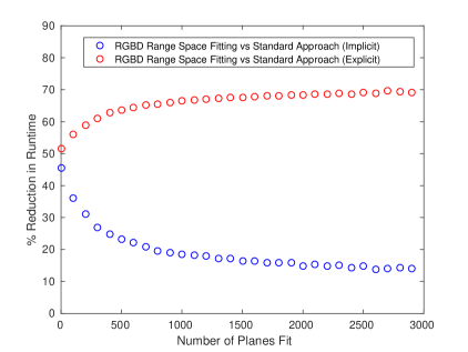
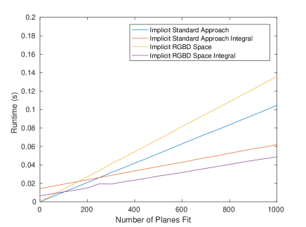
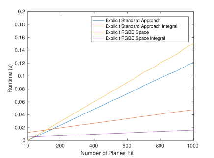
Fitting in RGBD range space has an advantage using this implementation due to the fact that integral images involving $\tan\theta_{x}(x,y)$ and $\tan\theta_{y}(x,y)$ can be pre-computed and do not change for a given sequence of range images. Therefore, fewer integral images need to be computed on a per image basis when compared to the standard approach using a similar integral image implementation. Fig. 3 compares the integral image implementations of both implicit and explicit RGBD range space fitting methods to their standard counterparts. For all integral methods, the time taken to compute the required integral images and fit a varying number of planes was compared. In the implicit case, integral image computation time was reduced by 45% and individual plane fitting time was reduced by ~15% compared to the standard approach. Using explicit fitting, integral image computation time was reduced by 52% and individual plane fitting time was reduced by ~70%. The reduction in integral image computation time is consistent with the analysis in § II-D and § II-E.

Figure 2: Runtime comparison of implicit and explicit fitting approaches using the integral image implementation. This data includes time taken to compute these integral images and perform a single plane fit with a varying number of points. Note that the time taken to perform these operations is constant despite the increasing number of points used in each fit.

Figure 3: Comparison of integral image RGBD range space plane fitting approaches vs integral image standard approaches for a single frame of depth image data. Computation of the integral images used in each method is included, with RGBD range space fitting approaches taking half as much time as time to compute the required integral images as their standard counterparts.

Figure 4: Depth image planar segmentation of a room corner featuring a blackboard and window. Depth image (left), color mapped depth image (middle), and segmented image (right). The algorithm successfully fit 268 planes on the 512x424 image. Tiles with successful plane fits are shaded and outlined in green. Tiles with too many invalid points or high fit error are outlined in red and blue respectively.

When performing implicit plane fitting in RGBD range space, precomputed values are used to fill the scatter matrix of equation (14) directly, leaving only the 4 elements that depend on $\frac{1}{Z}$ to be computed for each image. In contrast, the standard plane fitting approach requires computation of all elements of the scatter matrix from equation (6).

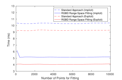
A similar implementation can be used for explicit plane fitting methods. When fitting in RGBD range space, there is a distinct advantage in terms of computation as the matrix elements of equation (16) do not depend on the measured depth data. This matrix depends only on the camera’s intrinsic parameters, and can be pre-computed. As shown in Fig. 2 and 3, these computational savings result in a 70% speedup in fitting planes for each measured image.

III-B Naive or “Standard” Implementation

The naive implicit fitting implementation computes the scatter matrix elements of equations (6) and (14) through the multiplication $\mathbf{M}^{t}\mathbf{M}$. When constructing each monomial vector $\mathbf{{M}}$, the standard approach requires two multiplication operations to obtain the X and Y values of the 3D points, while fitting in RGBD range space requires a single division to obtain the values $\frac{1}{Z}$. Fit times for both methods as a function of the number of points used is shown in Fig. 5. Results show that implicit fitting in RGBD range space is slower by ~15% compared to the standard approach when using this naive implementation. This unexpected time difference is attributed to the significant difference in computational cost between a multiply operation (~1-3 clock cycles on contemporary CPUs) and the divide operation (~10-20 clock cycles). The large discrepancy in the cost of the division dominates and the savings afforded by having half as many operations as discussed in §II-D and §II-E is superseded by this additional cost. Direct fitting using the disparity images which is directly proportional to inverse depth, $\frac{1}{Z}$, is very likely to alleviate these costs but investigation of these benefits is beyond the scope of this article.

Figure 5: Runtime comparison of implicit and explicit fitting approaches using the naive implementation (without integral image computation). For plane fits involving less than 10,000 points, explicit RGBD range space fitting is ~10% slower and implicit RGBD range space fitting is ~15% slower than the corresponding standard approaches.

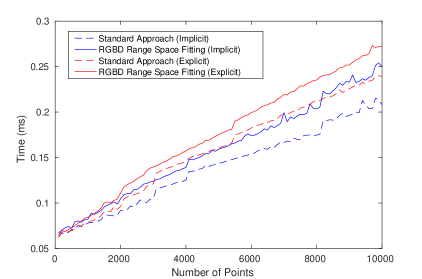
Similarly, the naive implementation of the explicit fitting approaches described in § I-D compute the matrices of equations (9) and (16) through the multiplication $\mathbf{M}^{t}\mathbf{M}$. Using the standard explicit fitting approach, the X and Y values of the 3D points must be computed to construct the monomial vector. Explicit fitting in RGBD range space requires no additional computation to construct the monomial vector, as values for $\tan\theta_{x}(x,y)$ and $\tan\theta_{y}(x,y)$ can be pre-computed. However, the vector $\mathbf{b}=1/[\begin{array}[]{cccc}Z_{0}&Z_{1}&\ldots&Z_{N}]\end{array}$ in this case, so values for $\frac{1}{Z}$ must be computed. We observed explicit fitting in RGBD range space to be ~10% slower than the standard explicit approach using this naive implementation.

III-C Integral Image vs. Standard Implementation Analysis

All implicit and explicit plane fitting methods were compared by examining runtime vs number of planes fit for a single depth image. Each plane was fit repeatedly to a 50x50 pixel subset of the overall image totaling 2500 points. For approaches involving integral images, computation of integral images was included in the overall runtime.

As shown in Fig. 6 in both the implicit and explicit cases, fitting in RGBD range space using an integral image implementation is faster than all other methods. Fitting 200 planes, implicit integral image RGBD space fitting takes 37% less time than the standard integral image approach and 28% less time than naive standard fitting. Explicit integral image RGBD range space fitting takes 62% less time than the standard explicit integral image approach and 50% less time than even implicit integral image RGBD space fitting.

Planar Segmentation Application

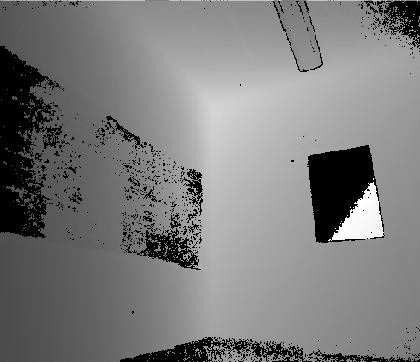
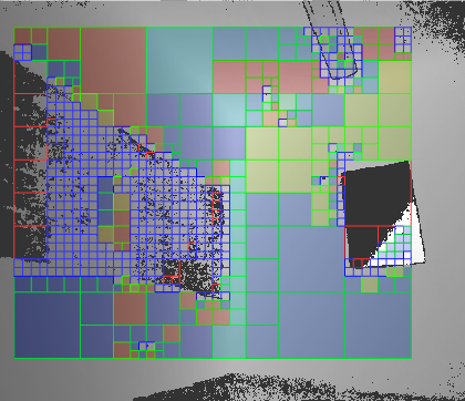
The integral image implementations of all plane fitting methods were compared by their application in a planar segmentation algorithm. The algorithm takes in a depth image and divides into an equally sized square grid. For each grid element, a plane is fit using each type of integral image plane fitting approach- integral image implementations of the standard and RGBD space fitting methods.

(a)

(b)

Figure 6: (a,b) compare performance of implicit (a) and explicit (b) plane fitting methods for a single depth image. As the number of planes fit per image grows larger, the integral image implementation of RGBD range space fitting quickly surpasses all other plane fitting methods in terms of speed.

If the error in the fit is above a threshold value, the grid element is subdivided into 4 equally smaller elements, each with half the width and height of the parent. This subdivision and plane fitting process is then repeated for these child grid elements, up to a maximum number of subdivisions. K-means clustering was then applied to planar coefficients to classify and label similar planes. This process results in the planar segmentation of the depth image as shown in Fig. 4.

For this algorithm, time spent plane fitting and computing integral images for 30 frames of depth image data was recorded. As previous analysis indicated, the integral image implementation of implicit RGBD range space fitting demonstrated significant time savings compared to its standard counterpart, taking 22% less time. In the explicit case, integral image RGBD range space fitting produced a 32% reduction in runtime compared to standard integral image fitting. Between the two fitting formulations, the explicit RGBD range space fitting approach was the fastest, taking 66% less time than implicit RGBD range space fitting. Extrapolation of these results indicate that over a five minute quadcopter flight the proposed algorithm would save over 30 seconds of processing time which may then be used for other on-board computational tasks.

IV Conclusion

The problem of real time surface fitting has shown itself to be an important challenge in the area of computer vision. In this work, we have introduced computationally efficient methods for least squares 3D plane fitting, which outperform the standard approaches when implemented using integral images. These methods improve upon existing approaches by separating the traditional fitting problem into components including the intrinsic camera parameters, which can be considered constant, and quantities related to the disparity of the incoming depth data.

This article proposed a reformulation of standard 3D plane fitting which, when coupled with integral imaging techniques, significantly reduces the computational cost associated with plane fitting to 3D point cloud data. We have also demonstrated the practical advantages in employing such methods in terms of a planar segmentation algorithm, which showed a substantial reduction in runtime consistent with other experimental results. We feel these results show promise for application of the proposed surface fitting methods in real time RGBD vision systems.

Future work may investigate a surface fitting approach dealing with the disparity data directly. After all, the quantity $\frac{1}{Z}$ is directly proportional to the sensed disparity. If depth information is not explicitly required, additional computational savings can be realized by working directly from measured disparities which may also eliminate the cost of depth computation which typically is performed by the sensor driver. It is also likely that surfaces of higher order can be estimated using a similar surface fitting formulation as proposed in this work, although it remains to be seen if such approaches would provide increased performance.

References

- [1] J. Han, L. Shao, D. Xu, and J. Shotton, “Enhanced computer vision with microsoft kinect sensor: A review,” IEEE Transactions on Cybernetics, vol. 43, pp. 1318–1334, Oct 2013.
- [2] D. Holz, S. Holzer, R. B. Rusu, and S. Behnke, “Real-time plane segmentation using rgb-d cameras,” in In Proc. of the 15th RoboCup Int. Symp, 2011.
- [3] K. Khoshelham and S. O. Elberink, “Accuracy and resolution of kinect depth data for indoor mapping applications,” Sensors, vol. 12, no. 2, p. 1437, 2012.
- [4] A. Fitzgibbon, M. Pilu, and R. B. Fisher, “Direct least square fitting of ellipses,” IEEE Trans. Pattern Anal. Mach. Intell., vol. 21, pp. 476–480, May 1999.
- [5] G. Taubin, “Estimation of planar curves, surfaces and nonplanar space curves defined by implicit equations, with applications to edge and range image segmentation,” IEEE Transactions on Pattern Analysis and Machine Intelligence, vol. 13, no. 11, pp. 1115–1138, 1991.
- [6] E. Trucco and A. Verri, Introductory Techniques for 3-D Computer Vision. Upper Saddle River, NJ, USA: Prentice Hall PTR, 1998.
- [7] Itseez, “Open source computer vision library.” https://github.com/itseez/opencv, 2015.
- [8] R. B. Rusu and S. Cousins, “3D is here: Point Cloud Library (PCL),” in IEEE International Conference on Robotics and Automation (ICRA), (Shanghai, China), May 9-13 2011.
- [9] C. Erdogan, M. Paluri, and F. Dellaert, “Planar segmentation of rgbd images using fast linear fitting and markov chain monte carlo,” in 2012 Ninth Conference on Computer and Robot Vision, pp. 32–39, May 2012.
- [10] T. J. J. Tang, W. L. D. Lui, and W. H. Li, “A lightweight approach to 6-dof plane-based egomotion estimation using inverse depth,” in Australasian Conference on Robotics and Automation, 2011.
- [11] J. P. Lewis, “Fast template matching,” in Vision interface, vol. 95, pp. 15–19, 1995.
- [12] P. Viola and M. Jones, “Rapid object detection using a boosted cascade of simple features,” in Proceedings of the 2001 IEEE Computer Society Conference on Computer Vision and Pattern Recognition. CVPR 2001, vol. 1, pp. I–511–I–518 vol.1, 2001.