A bridge between invariant dynamical structures and uncertainty quantification
Abstract
We develop a new quantifier for forward time uncertainty for trajectories that are solutions of models generated from data sets. Our uncertainty quantifier is defined on the phase space in which the trajectories evolve and we show that it has a rich structure that is directly related to phase space structures from dynamical systems theory, such as hyperbolic trajectories and their stable and unstable manifolds. We apply our approach to an ocean data set, as well as standard benchmark models from deterministic dynamical systems theory. A significant application of our results, is that they allow a quantitative comparison of the transport performance described from different ocean data sets. This is particularly interesting nowadays when a wide variety of sources are available, since our methodology provides avenues for assessing the effective use of these data sets in a variety of situations.
1 Introduction
Uncertainty Quantification (UQ) searches for a quantitative characterization of uncertainties in computational models of real-world applications. Uncertainties associated to these models have been studied for many years. Depending on the context they can arise as a result of noisy or incomplete data, errors introduced by numerical models, or by the lack of complete understanding of the governing physical processes.
In geophysical contexts, uncertainty is a topic of much interest because it is inherent to the equations describing the motion of fluids such as the ocean or the atmosphere. The motivation of this paper is trying to acquire a deeper understanding of uncertainty quantification, that allows a better characterization of its presence in ocean models. Large amount of oceanic data are becoming now available. For instance, the Copernicus Marine Environment Monitoring Service (CMEMS) provides regular and systematic information about the physical state and dynamics of the ocean for the global ocean and the European regional seas. The data cover the current and future state of variables and the provision of retrospective data records (re-analysis). Other oceanic services include ocean currents supplied by altimeter satellites, like AVISO; the HYbrid Coordinate Ocean Model (HYCOM), a consortium, which is a multi-institutional effort sponsored by the National Ocean Partnership Program (NOPP), as part of the U. S. Global Ocean Data Assimilation Experiment (GODAE), to develop and evaluate a data-assimilative hybrid coordinate ocean models, etc.
Ocean models are built on partial differential equations, which are only an approximation of reality. Indeed, typically ocean models approach ocean motion by the Reynolds-averaged Navier-Stokes equations using the hydrostatic and Boussinesq assumptions. In this context inaccurate or inadequate models lead to structural uncertainty. Even if these equations were perfectly accurate models, they contain parameters, such as viscosity or diffusivity, which are not known precisely and cause parameter uncertainty. Boundary conditions on input variables, lead to parametric variability. For instance input variables such as velocities, experience at the surface atmospheric winds, which impose forcings on the velocities, and these atmospheric forcings are not precisely known. Eventually these models are not solved exactly, but numerically through discretization methods and numerical approximations, which are subjected to numerical errors, and causes algorithmic uncertainty. For all these reasons, the predicted ocean currents are also uncertain. Uncertainties in the solutions, system outputs, due to the uncertainties in the system inputs is referred to as forward uncertainty quantification [1].
In this work, we are interested in evaluating the reliability of the outputs, ocean currents, regarding the transport they produce. This is a perspective slightly different to the classical one now described, in which ocean models adequacy is judged just against the velocity fields. Transport in the ocean surface is produced by fluids parcels that follow trajectories that evolve according to the dynamical system:
| (1) |
where the position is described in longitude () and latitude () coordinates, that is, , and represents the velocity field, which has two components determined by the zonal () and meridional () velocities. In longitude/latitude coordinates, the dynamical system in Eq.(1) can be rewritten as:
| (2) |
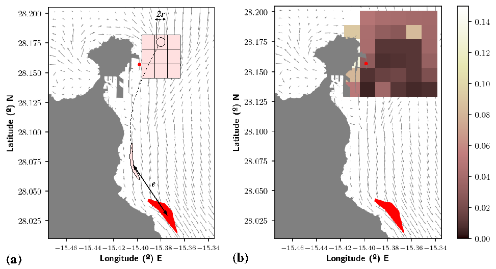
where is the Earth’s radius. The system (1), which is a general expression encompassing the specific problem dealt with in (2), is a nonlinear non-autonomous dynamical system in 2D. Uncertainties in the velocities , or more generally in the vector field, produce uncertainties in the solutions . In general, as illustrated in figure 1, the exact model connecting two successive observations is not known. Only the initial observation, , and the final state, , are measurable. They are presented in red color in the figure. The evolution of initial conditions, , in a neighbourhood close to the initial observation, , towards a final state, , predicted by a model is expressed in the pink color in the same figure. The uncertainty of the model in representing the observations can be expressed in a number of ways. It may be defined by an absolute error , which measures distance, in a certain metrics, between the final observation , which is considered a target and the computed prediction . This work proposes measures for this error and links the proposed uncertainty quantifier with dynamical objects present in the model (1). This is done without making any mathematical assumption about the observations.

This paper is structured as follows. In section 2, we will discuss and develop an approach to uncertainty quantification recently taken for an ocean study case in [2]. We will show evidence of connections between the introduced definitions and the dynamical objects of system (1). In section 3, we will provide formal results to show how, for specific simple examples of the system (1), the definition of uncertainty quantification given in section 2, is able to highlight these dynamical objects. These results support one of the main findings of this article which is that stable invariant manifolds of hyperbolic trajectories provide a structure to forward uncertainty quantification. We will see in detail what is meant by this statement. Section 4 presents a discussion with further examples that illustrate the findings of this work and links uncertainty quantification to Lagrangian Descriptors and other Lagrangian indicators found in the literature. Finally, in section 5, we will provide the conclusions.
2 Transport uncertainty quantification in ocean models
In this section, we propose uncertainty quantification metrics. We work in the context of transport in ocean models, starting the discussion from the results presented in [2], which considers the performance of very high resolution tools for the monitoring and assessment of environmental hazards in coastal areas. In particular, this work, following the scheme presented in figure 1, quantifies uncertainties of several high resolution hydrodynamic models in the area of Gran Canaria, by measuring an error between the observations and predictions for the evolution of a diesel fuel spill event, well documented by port authorities and tracked with very high resolution remote sensing products. The pollution event was produced after the collision of the passenger ferry ‘Volcán de Tamasite’ with the Nelson Mandela dike in La Luz Port on April 2017. After the crash, supply pipes along the dike were broken and diesel fuel poured into the sea. SAR Sentinel 1 images were available in the area approximately one day and a half after the accident from which it was possible to identify the spill. For that period ocean currents in the area were available from two sources. One was the Copernicus Marine Service model for the Iberian-Biscay-Irish region (CMEMS IBI-PHY, IBI hereafter) and other was a very high resolution model of Puerto de la Luz setup by Puertos del Estado currently implemented and running operationally in different Spanish Port Authorities within the SAMOA port forecast system [3]. In [2], for each model, uncertainties are quantified by measuring an error with respect to a target, a ‘ground truth’, which should be recovered by the model. In particular, following the scheme proposed in figure 1, figure 2 illustrates how the uncertainty quantifier metrics is proposed. The ferry impact point, the Nelson Mandela dike, which is marked with the red dot, represents an initial observation. The currents represented in the background are the ones obtained from the model set by Puertos del Estado at day . The elongated red blob represents the spill as identified from satellite images one day and a half after the accident. This is the target observation, the ‘ground truth’. In panel (a) a set of initial conditions, , are selected in the neighbourhood of the initial observation and marked in a rectangular pink domain. This domain is divided into sub-domains and in each one a small circular blob with radius , is evolved in a time interval from the initial time . This is represented just for one of the sub-domains. The blob distorts while it approaches the target observed spill. A way to measure the ‘proximity’ between the blob and the target spill at the final time, , is to compute the distance between the centroid of the evolved blob, (), and that of the observed spill, (). Mathematically this can be expressed as:
| (3) |
Here, denotes the modulus of the vector. The position of the centroid of the evolved spill, , depends on time t, while the centroid of the ground value slick does not, because it is an observation at a final time, . The centroid of a finite set of points is defined as:
| (4) |
where are the (lon, lat) coordinates that define the contour of the slick in an equirectangular projection. The solid black line in panel (a) is the distance between centroids of the modelled and observed blobs. This is the value taken by Eq. (3). The procedure is repeated for additional circles centered in different positions of the sub-domains or cells, in the neighbourhood of the accident place. The evolution of each of these circular blobs is different due to the chaotic nature of transport in this setting. Panel (b) in figure 2 provides a visualization on how this calculation changes in each sub-domain. This panel represents a colormap which is placed in the port neighbourhood, at the same position than the pink domain in panel (a). It considers a mesh-grid, and the colorcode within each cell represents the value of Eq. (3) obtained for blobs with initial positions in the center of each cell and initial radius of . We observe a nonuniform distribution.
a)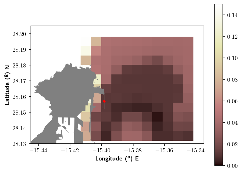 b)
b)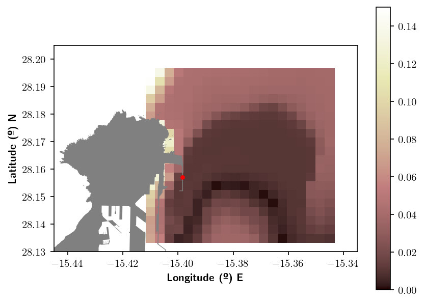
a)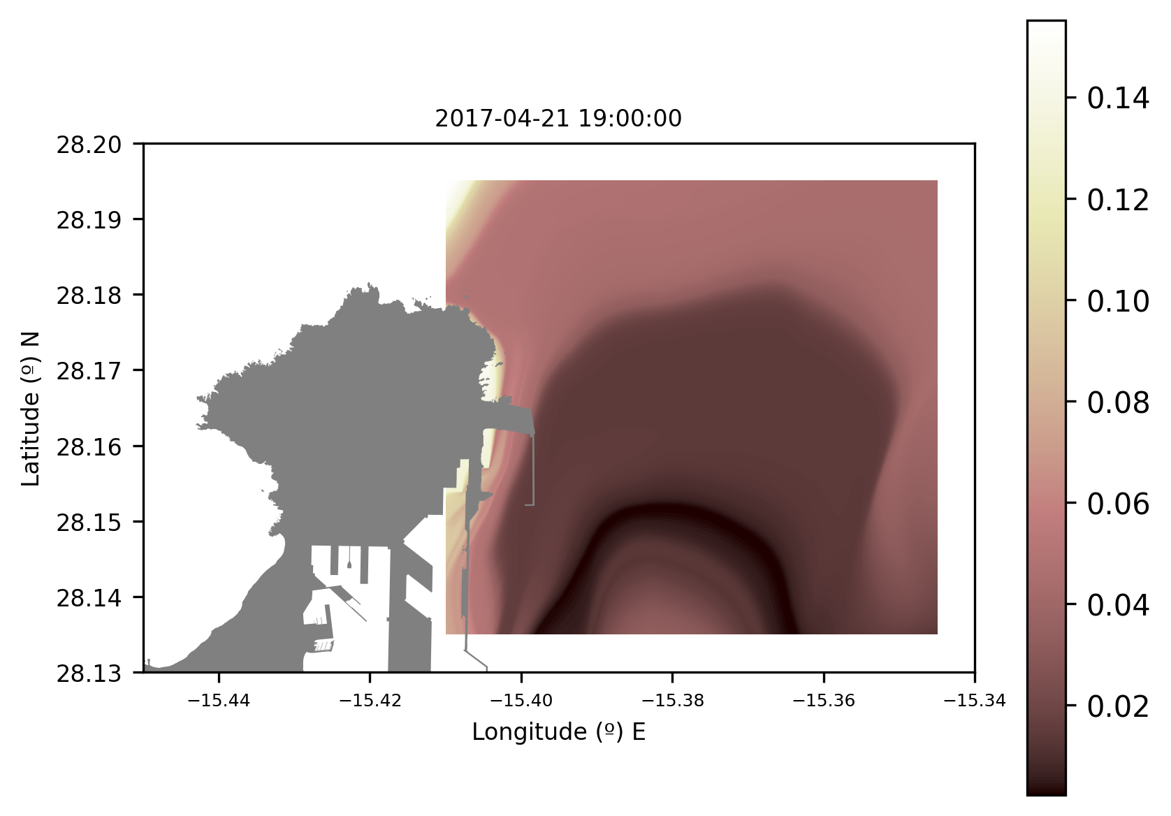
b)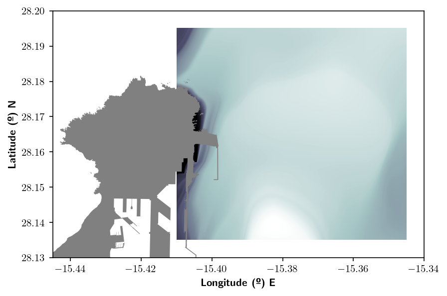 c)
c)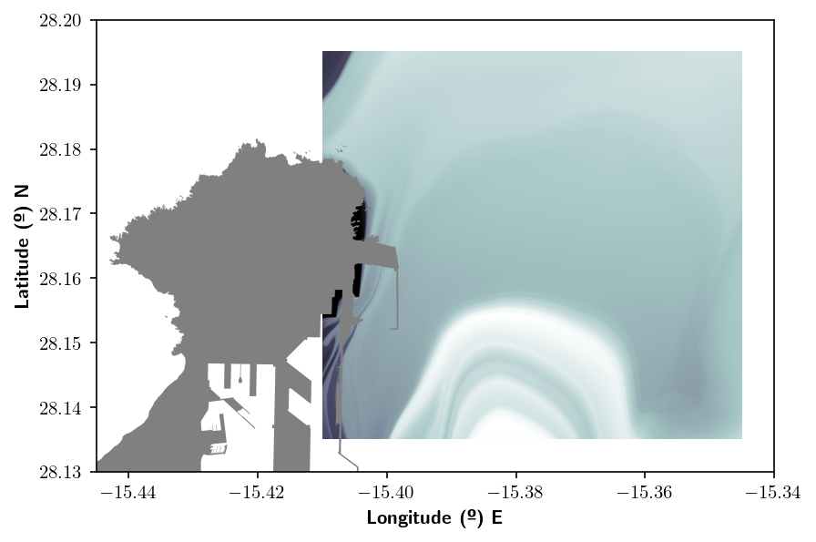
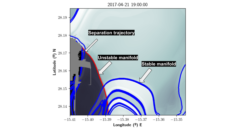
Figure 3 expands results of Figure 2b) by increasing the number of cells in the neighborhood domain and decreasing the radius of each initial blob. In particular, Figure 3 a) considers a mesh and initial blobs with radius . Figure 3 b) increases the number of cells to a mesh-grid and decreases the radius of initial blobs to . Figure 3b) makes visible an underlying structure which is directly related to the invariant dynamical structures, as we will shown later. In the limit , expression (3) is rewritten as:
| (5) |
where is a trajectory of a fluid parcel, a solution to the system (1), with initial position at each cell in the grid. Figure 4a) illustrates the results of this calculation in a very fine grid.
One of the goals of this paper is to establish connections between the uncertainty quantifier (5) and invariant dynamical objects that control transport in vector fields. These are geometrical objects that organize particle trajectories schematically into regions corresponding to qualitatively distinct dynamical behaviors. In the context of fluid dynamics these objects are referred to as Lagrangian Coherent Structures (LCS). An essential ingredient of the LCS are hyperbolic trajectories characterized by high contraction and expansion rates. Directions of contraction and expansion define, respectively, stable and unstable directions, which are, respectively, related to the stable and unstable manifolds. In the context of the ocean model and the event described above, Garcia-Sánchez et al. have shown in [2] that there exists a hyperbolic trajectory located on the coastline very close to the accident point, in a detachment configuration, which is related to the phenomena of flow separation. Under this configuration, the stable manifold of the hyperbolic trajectory is aligned with the coast, and the unstable manifold is transversal to it. Figure 5 illustrates, respectively, in blue and red the stable and unstable manifolds of the separation trajectory for this particular case that we studied. Any blob placed in the neighbourhood of the separation trajectory, eventually evolves to become aligned with the unstable manifold, which is an attracting material curve. The configuration of the unstable manifold in Figure 5, is consistent with the observed spill marked in red in Figure 2. Indeed, the observed spill has evolved to be completely aligned with the unstable manifold. The invariant dynamical structures displayed in Figure 5 have been obtained by means of the Lagrangian Descriptor [4, 5, 6], which measures arc-length of trajectories:
| (6) |
In [7], for some generalizations of the expression (6), is proved that stable and unstable manifolds are aligned with singular features of this function. The forward integration highlights the stable manifold, while the backwards integration highlights the unstable manifold. In this work the notion of singular feature is related to an undefined directional derivative in a direction transverse to the manifold curve. In Figure 5, red and blue features are placed on the singular features of .
The metric given in (5) posses similarities with the forward definition of the function :
| (7) |
The analogy between structures obtained from expressions (5) and (7), is confirmed from figure 4. Panel a) displays expression (5) results, while panels b) and c) display Eq. (7) results for and 2 days respectively. Figure 4 highlights singularities both for the forward uncertainty quantifier and for the forward function. From this figure is clear that Uncertainties displayed in panel a) reach minimum values along the stable manifold. Indeed, the stable manifold is an optimal pathway towards the unstable manifold, which in turn is an attracting material curves towards which all fluid parcels evolve. In this case, as the observed evolution of the spill is aligned with the unstable manifold, it is expected that minimum values of the uncertainty quantifier correspond to the stable manifold. On the other hand indicators of structural uncertainty that show inadequacy of the model, would correspond to situations in which these minimum values are not reached along the stable manifolds. This would have been the case if, for instance, the observed spill would have been found far from the unstable manifold.
3 Formal results
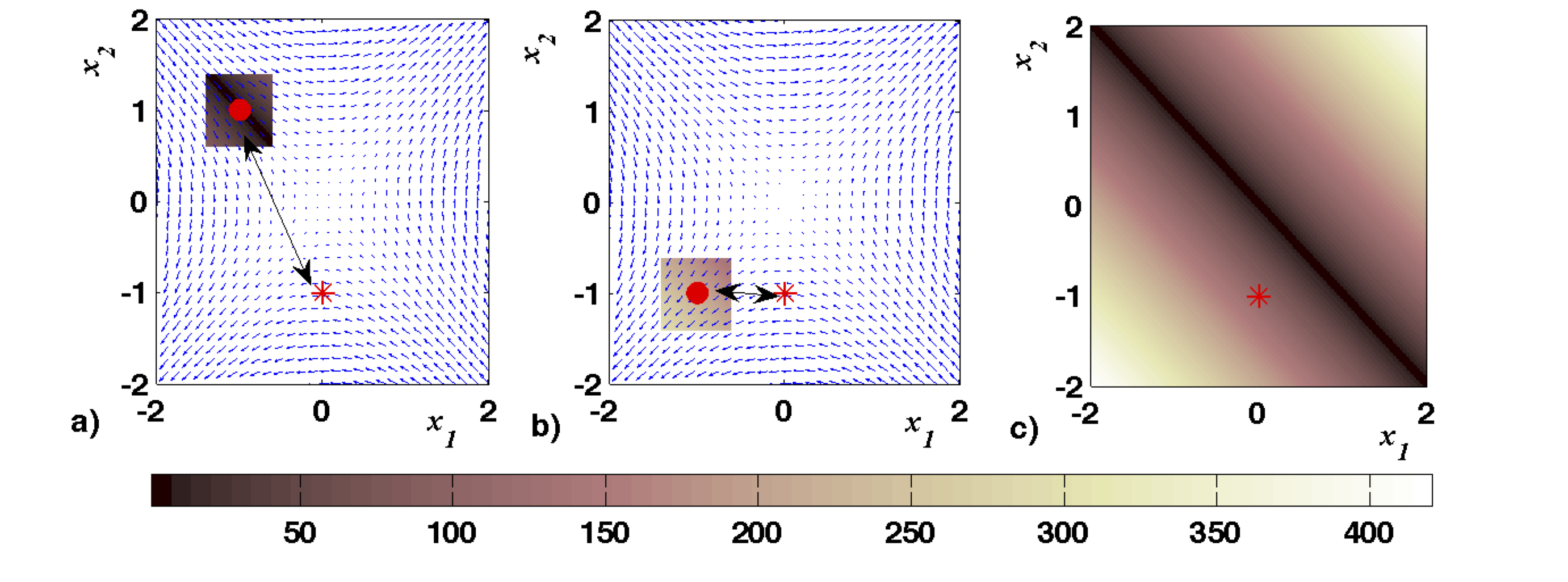
This section is focused on illustrating the analogies found in figure 4 between the pattern in panel a), which is related to uncertainty quantification, and those in panels b) and c), which are related to stable invariant manifolds. For the event described in the previous section computations in panel a) are performed with the measure proposed in Eq. (5) to quantify uncertainty in a neighbourhood of the accident location. When the calculation is performed on a very fine grid it is found that the uncertainty has a structure that is related to that of invariant stable manifolds. In order to find answers to the question of why there are singular structures obtained from the expression (5) that are aligned with invariant stable manifolds of hyperbolic trajectories, we need to assume an explicit expression for the vector field in Equation (1). Indeed in the example discussed in the previous section, velocities are given as data-sets and this makes difficult to proceed with exact calculations. In this way, in this section we perform an analysis in simplified planar vector fields with exact explicit expressions. Figure 6 displays such example. In panel a) an initial observation at time is marked with a red circle. At a later time, , this observation is at the target position marked with a red asterisk. We model this evolution with the vector field at the background, which is represented at time . In order to quantify the uncertainty in the neighbourhood of the initial observation, we display the evaluation of around it. The colorbar placed at the bottom of the figure, measures the uncertainty in the domain units. This colorbar indicates that uncertainties in this neighbourhood are low. At least lower than those displayed for the experiment in panel b). In this case the initial observation is at a different position, although the target is kept at the same position than in a). In this case uncertainties are larger, indicating that the vector field in the background is not a good model to express the transition between these two observations. Finally panel c) displays evaluated in the whole domain. This expresses the uncertainty associated to the planar flow, assuming that observations start in different points of the representation domain and that they evolve towards the assumed observed target position at the red asterisk. The panel confirms that model has a better performance for those initial observations placed at the diagonal. Results presented next in this section are displayed following this type of representation.
Our analysis in this section follows the spirit of the work by [6, 7, 8, 9]. We assume the definition of singular features given there, by considering that these are features of on which the transversal derivative is not defined. We will prove, for simple selected examples, that stable manifolds are aligned with those singular features of .
Finally, before beginning our discussion the definition (5) is generalized as follows:
| (8) |
Here, is the initial condition of the trajectory . In the particular case described in the previous section , which corresponds to the ocean surface, and . The coordinates of the target are An alternative for this expression that we will use is the following:
| (9) |
3.1 The autonomous saddle point
The first example that we analyze is the vector field that corresponds to the Hamiltonian linear saddle case for which , satisfying and the equations of motions are:
| (10) |
where . For any initial observation , we consider the unique solution of this system passing through the condition , which is:
| (11) |
For this example, the origin is a hyperbolic fixed point with stable and unstable manifolds:
| (12) |
| (13) |
For simplicity we assume, without loss of generality, that (this is possible for autonomous systems). We consider the target in the position and apply (11) to (9) to obtain:
Regrouping terms, we get
| (14) |
In this expression, , which always satisfies . We explore separately the first and second terms. For the factor there exists a such that if , then and . This is always the case for and is a plausible assumption for , if . We recall that and that therefore such exists if . In this case positiveness is guaranteed for sufficiently large , i.e, a Taylor series around , attained if and , is performed for the binomial:
Therefore,
We recall that and . This yields,
We analyse next the second term in Eq.(14). The sign of depends crucially on the sign of given that for the term can be as small as we like. Let us consider such that if and , then . The following is valid for above this lower value:
Therefore, when , and ,
| (15) |
Now, we consider and satisfying . Therefore:
Therefore, when , and ,
| (16) |
Finally, we conclude that
| (17) |
Therefore, since
Thus, we can approximate as
| (18) |
where the dominant term is . Hence, to leading order, the stable manifold at is aligned with a singular feature of for ‘sufficiently large’ . This statement however must be considered in the sense that expression expresses a good approximation for as far as , and that for any is valid for a sufficient large satisfying, .
We have shown that Eq. (9) is able to highlight the stable manifolds for the autonomous saddle point. Next, we analyse what happens when we consider Eq.(8), and in which cases it provides information about the stable manifold of the autonomous saddle point. When we apply (11) to (8), it yields
We remark that our following calculations will be restricted to and integer. Rewriting the expression for
| (19) |
Recalling that , and that for sufficiently small , i.e. sufficiently large , and the case and , a Taylor series around , for integer number, for the second factor:
| (20) |
Alternatively, considering the case and , a Taylor series around for the second factor is as follows:
| (21) |
Therefore in general:
| (22) |
We notice that since , the terms have positive exponents and if in principle are much smaller than the first term and therefore:
| (23) |
Hence, the stable manifold at is aligned with a singular feature of this approximation to for ‘sufficiently large’ . This statement though, must be considered with care, because in Eq. (22) the terms in are multiplied by which has a negative exponent, and therefore have a singularity at . For this reason neglecting these terms versus the first one if we are very close to would require checking that the products, such as, are really small. This implies that Eq. (23) is correctly approximating for as far as we are sufficiently away from 0 in , i.e. . In practice this condition is satisfied for any grid used in later figures that exclude . Also we can state that for sufficiently large , is very close in almost all the domain to the function given in Eq. (23), which possess a ”singular feature” aligned with the stable manifold. Fig.7 a) and b), illustrates how the stable manifold is aligned with singular features of the Lagrangian uncertainty quantifier defined either by Eq.(8) or (9).
a)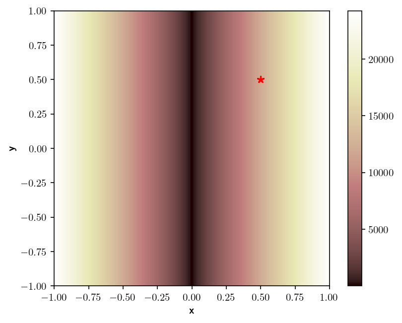 b)
b)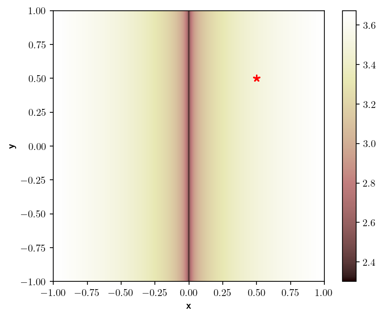
3.2 The autonomous rotated saddle point
This second case that we explore is the vector field of the rotated linear saddle for which the equations of motion are:
| (24) |
The general solution to this system is:
| (25) |
where and depend on the initial conditions and as follows:
Here, corresponds to the stable manifold of the hyperbolic fixed point placed at the origin and corresponds to its unstable manifold.
For any initial observation and final target observation , we introduce the solution (25) into Eq.(9) obtaining:
| (26) |
We expand next the first term in Eq.(26). In particular, we consider the case in which for which it is always possible to find a in which :
Here we have used . The Taylor expansion of the binomial when , i.e., when , is
Therefore,
Since , for when . Hence,
By removing the change of variable, we obtain
| (27) |
We consider now the case that implies for some sufficiently large . The Taylor series is the same, except for a minus sign. It yields,
| (28) |
Finally,
| (29) |
We analyse next the second term in Eq.(26). As before, we start considering the case and . After making the change of variable we obtain:
Since , for when . Hence,
By removing the change of variable, we obtain:
| (30) |
We compute the same term but in the case . The Taylor series is the same, except for a minus sign. It yields,
| (31) |
Finally,
| (32) |
Thus,
| (33) |
The stable manifold at is aligned with a singular feature also at .
As for Eq.(8) considering , and leads:
| (34) | |||||
As before the leading term in leads to:
| (35) |
and similar considerations apply in neglected terms to the ones made for Eq. (22), but now regarding to singularities at . Fig.8 a) and b), illustrate how the stable manifold is aligned with singular features of the Lagrangian uncertainty quantifier defined either by Eq.(8) or (9).
a)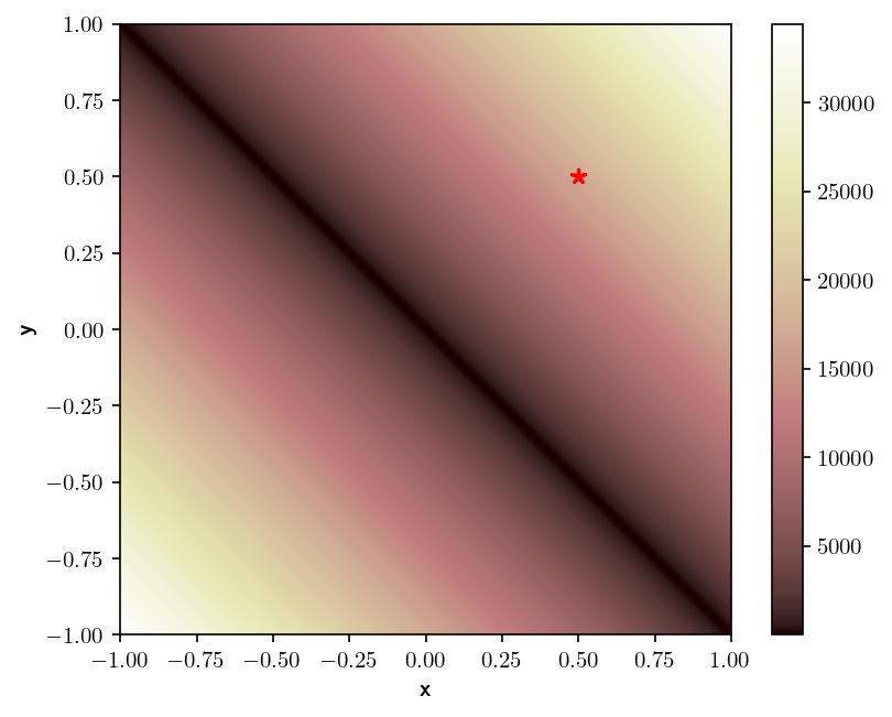 b)
b)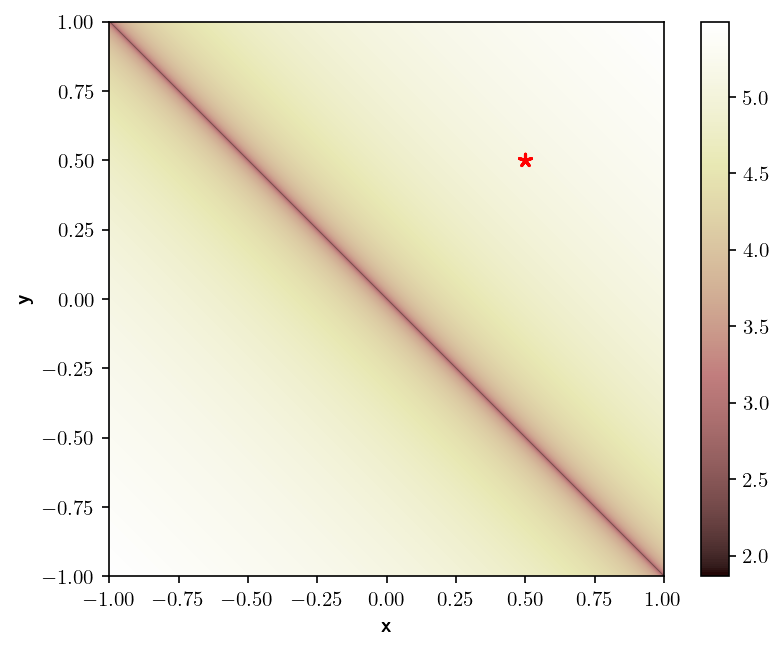
3.3 Discrete maps
These findings in the previous two subsections can be easily extended to discrete time dynamical systems, which are also useful in applications. Discrete time dynamical systems are defined as maps.
The autonomous saddle point
Consider the following linear, area-preserving autonomous map:
| (36) |
For an initial condition , the unique solution of this system is:
| (37) |
As for the continuous time case, the origin is a hyperbolic fixed point with stable and unstable manifolds:
| (38) |
| (39) |
We apply (37) to (9) to obtain:
| (40) |
Regrouping terms, we get
| (41) |
Considering that the transformation can be directly applied to all the calculations performed in the continuous time case, we recover from Eq.(14):
| (42) |
When , the dominant term is . Hence, the stable manifold at is aligned with singular features of for ‘sufficiently large’ iteration .
The same is applicable to (8). It yields,
| (43) |
We note that the stable manifold at is aligned with singular features of for a ‘sufficiently large’ iteration . The same issues as before regarding singularities on the manifold position apply.
Fig.9 a) and b), illustrate how the stable manifold is aligned with singular features of the Lagrangian uncertainty quantifier defined either by Eq.(8) or (9).
a)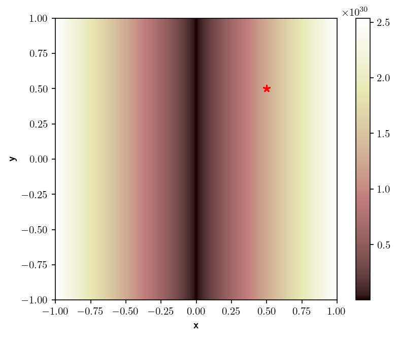 b)
b)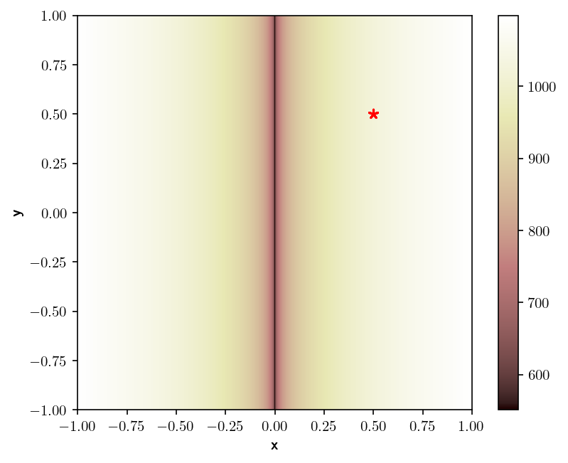
The autonomous rotated saddle point
We consider the following discrete dynamical system:
| (44) |
It is easy to see that the stable and the unstable manifolds are given by the vectors and respectively. The solution of this system yields to,
| (45) |
where
Again considering the transformation and the use of previous results for the continuous time case, we recover from Eq.(33):
Therefore, the dominant term is
Since , there is a singular feature at , i.e., in the subspace generated by . Hence, the stable manifold is aligned with a singular feature of .
The same is applicable to (8). It yields,
Hence, the stable manifold is aligned with a singular feature of . Fig.10 a) and b), illustrates how the stable manifold is aligned with singular features of the Lagrangian uncertainty quantifier defined either by Eq.(8) or (9).
a)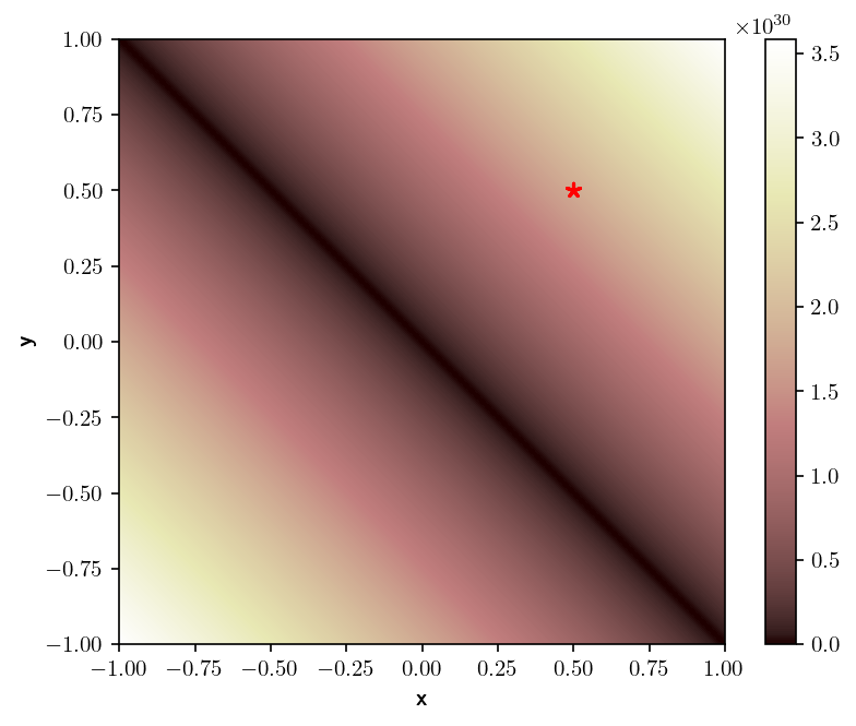 b)
b)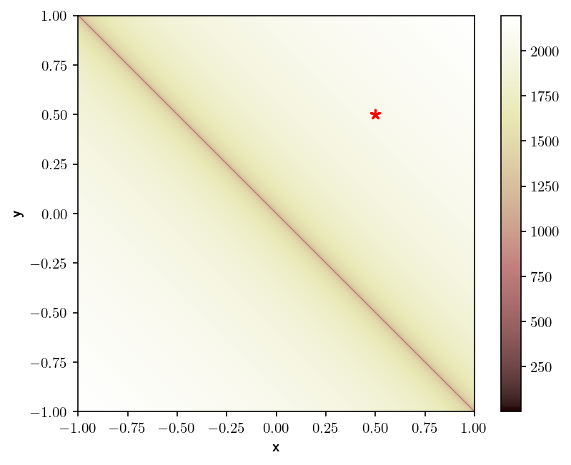
4 The Duffing equation
Results in the previous sections are generalized to the autonomous nonlinear case by means of the Moser’s theorem [10]. This theorem applies to analytic two-dimensional symplectic maps having a hyperbolic fixed point or, similarly, to two-dimensional time-periodic Hamiltonian vector fields having a hyperbolic periodic orbit (which can be reduced to the former case considering a Poincaré map). The case of a Hamiltonian nonlinear autonomous system is a one-parameter family of symplectic maps, and therefore Moser’s theorem applies. Following proofs sketched by [8, 7] results may be extended to the case of non-autonomous nonlinear dynamical systems by utilizing results like the Hartman–Groman theorem.
This section discusses further results on the Lagrangian Uncertainty Quantifier by considering the evaluation of (8) over a vector field obtained from the nonlinear periodically forced Duffing equation:
| (46) |
Prior to discuss outputs of (8) into Eq. (46), we discuss the structure of invariant manifolds of hyperbolic trajectories in Eq. (46) for the case and the persistence versus this time dependent perturbation of tori present in the unforced version of Eq. (46), i. e, . In the perturbed case, the hyperbolic fixed point placed at the origin, becomes a hyperbolic periodic trajectory [4], and their stable and unstable manifold can be highlighted by the Equation 6 appeared in Section 2 [6]. Additionally, as discussed in [7] a scale factor applied to (6) converts the expression to an average, which in compact Hamiltonian systems like (46) converges for and when this convergence is observed, level curves correspond to invariant structures of the dynamical system. Convergence of means are computationally verifiable on tori, however on hyperbolic sets as discussed in [9], rounding computational errors practically prevent convergence.
a) 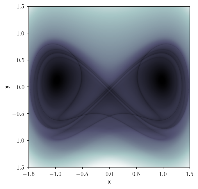 b)
b)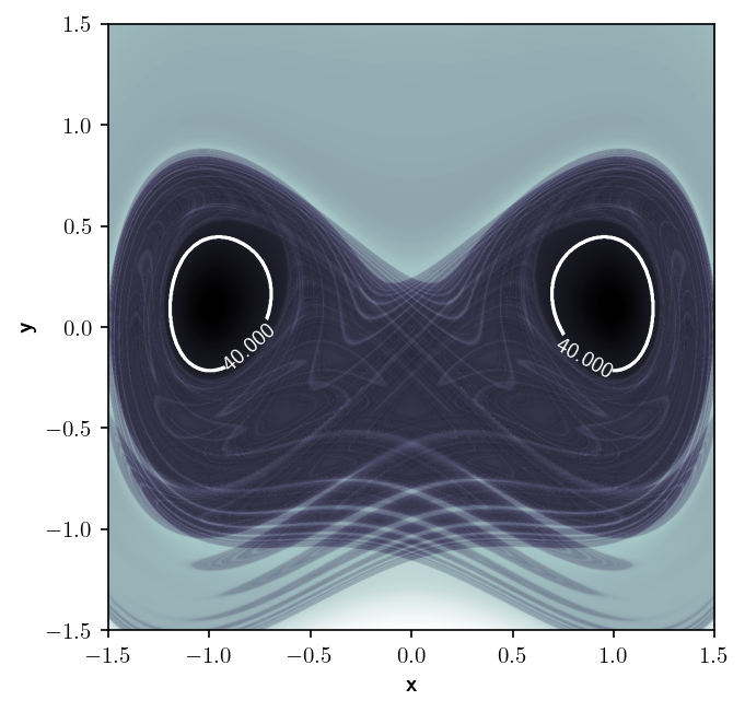
Figure 11 illustrates these points. Panel a) shows invariant manifolds related to the hyperbolic trajectory that are obtained from (6) for . These structures become much more rich for larger as panel b) confirms. In this panel since the average of has converged in the smooth region, level curves in the area highlight tori. The outputs of Figure 11a) may be split into two figures, by separating the backwards and forwards integration of Eq. (6), which displays, respectively, the unstable and stable manifolds. These outputs are depicted, respectively, in Figure 12a) and b).
a) 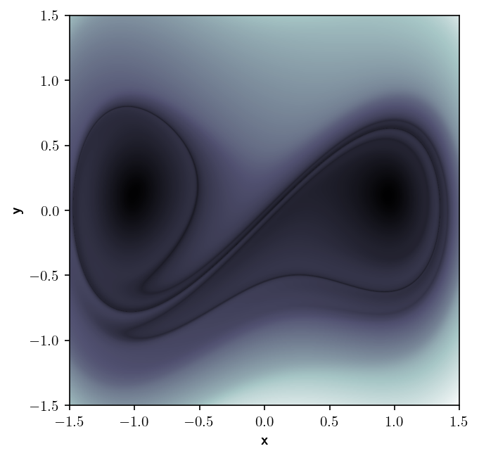 b)
b)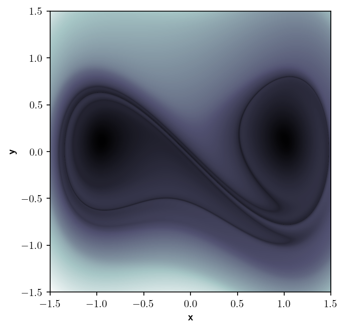
Figure 13 shows the evaluation of as in Eq.(8) with for , and different targets. In panel a) the chosen target is . This target is within the chaotic region displayed in Fig. 11b), close to the unstable manifold of the Duffing equation. It is observed that minimum values are reached on the stable manifold and that the structure of is correlated to it. This setting is similar to what was observed for the ocean case described in Section 2, in which the observed oil evolution is aligned with the unstable manifold and minimum values of are found on the stable manifold that are optimal pathways towards the unstable manifolds. In panel b) we show the results for the target which is within the right tori like structure highlighted in Fig. 11b). Accordingly, uncertainty values are very low for initial observations in the corresponding tori region, but very high for the tori like region at the left side. Indeed initial observations in this region will never go near a final observation in the right tori like structure, and therefore this model is structurally uncertain for those observations, i.e. the model is inadequate to represent those. Panel c) shows the computation of the uncertainty for a target outside the geometry of the unstable invariant manifold displayed in Fig. 12a). It is remarkable the persistence in all these examples of an structure on the uncertainty field with singular features linked to the stable manifold independently of the target value .
a)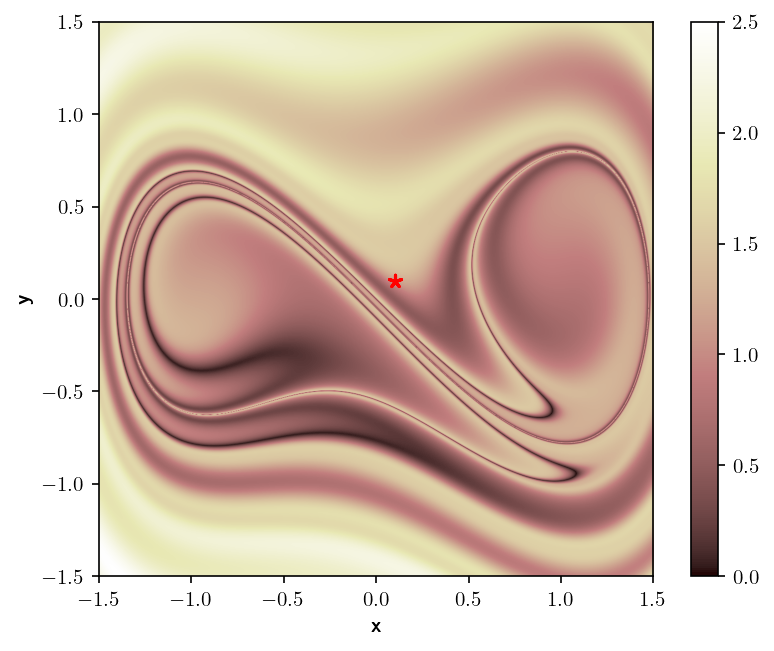 b)
b) 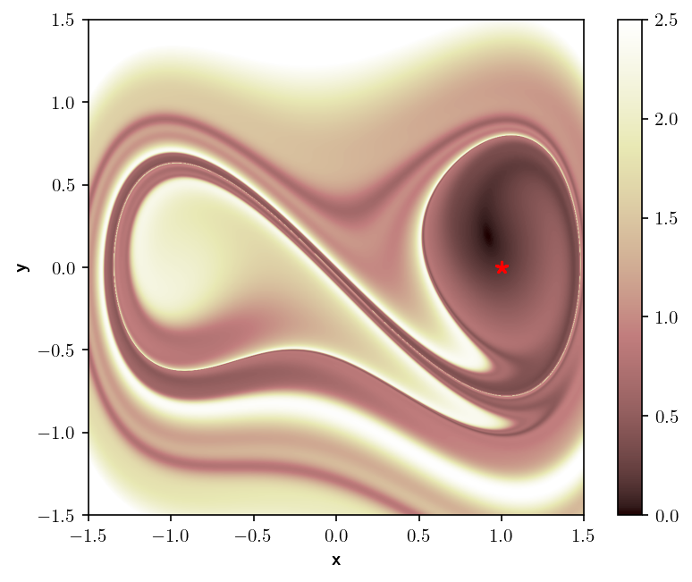 c)
c)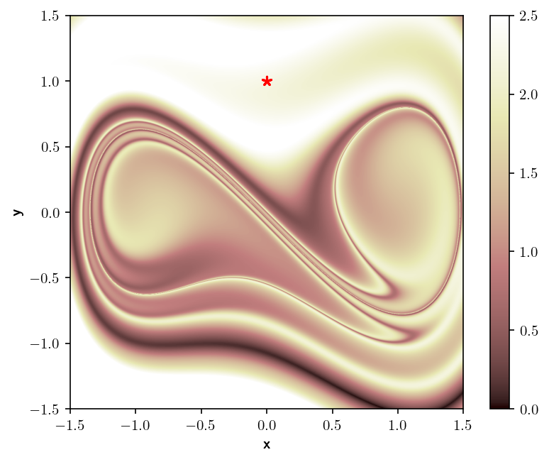
a) 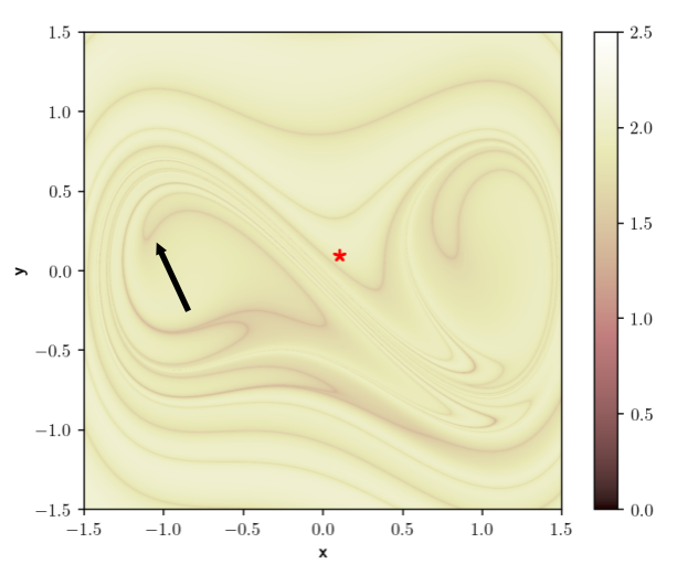 b)
b)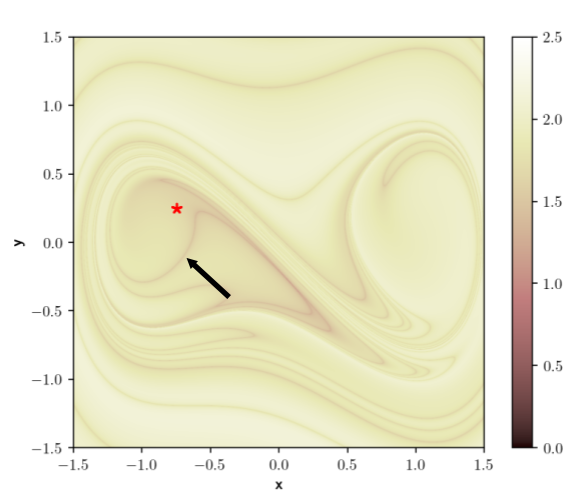 c)
c)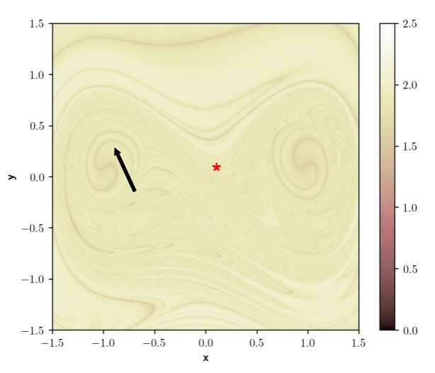
Figure 14 shows the evaluation of Eq.(9) with , and different targets or integration periods. Panels a) and b) have the same integration periods, but different targets. In them the black arrow points out different spurious features that seem singular but do not correspond to any invariant manifold. Figure 14 c) shows the same than panel a) for an integration period of 50. The black arrow marks a region, which from the analysis of Fig. 11, is known to be covered by tori, while the structure attained from Eq.(9) does not highlight this. Indeed, the ergodic partition theory discussed in [11, 12] and implemented in [7] for Lagrangian Descriptors such as that in Eq. (6), shows that this ability to highlight tori, requires averaging along trajectories, while expressions Eq. (8) or (9) are not averages, and therefore do not qualify for the application of ergodic principles. These expressions are not suitable for identifying this kind of invariant objects.
5 Discussion
There is much interest in uncertainty quantification involving trajectories in ocean data sets. Recent efforts in this direction are [13, 14, 15, 16]. Vieira et al. [16] have developed a clustering method to partition the space of trajectory data sets into distinct flow regions. This method contains free parameters and they use uncertainty quantification to assess the parameter dependence on the partitions they obtain. The work [15] discusses approaches for uncertainty quantification from a geometrical perspective, and uncertainty quantifiers based on distances are proposed, but no connections are proposed with invariant dynamical structures. Similarly in [14] uncertainty quantifiers based on a descriptive statistics of distances between modelled trajectories and observations are used, but no relations are presented between these and the invariant dynamical structures. Results appeared in [17] also discuss along these lines, but in the context of general models, not related to ocean data. In this work authors have established links between uncertainty quantification and invariant manifolds under explicit mathematical assumptions for the ”true” model. The results in our work do not require such assumptions.
Equations similar to (8) or (9) have been used in the literature to highlight Lagrangian structures in oceanic flows. For instance [18, 19] have done so. Prants in [18] proposed to use the arc-length to study the displacement of particles in the coasts of Japan.
| (47) |
Here, represents the relative displacement of a particle from its initial position to certain final one . This expression is the analogue to Eq.(8) with and target adjusted to each initial condition. However, in this work no connections are established between Eq. (47) and uncertainty quantification.
6 Conclusions
This article explores the implications of a definition for Uncertainty Quantification recently proposed in oceanic contexts [2]. It is found that for this definition, which is associated to forward Uncertainty Quantification, stable invariant manifolds of hyperbolic trajectories of the underlying flow, provide a structure for it. That is, we found that the proposed Uncertainty Quantifier is a function that contains a very rich structure, which is related to these well known structures from dynamical systems theory. For selected examples this statement has been proven. Also examples are discussed in which singular structures of the Uncertainty Quantifier highlight spurious structures, not aligned with invariant features of the dynamical system. Other invariant structures like tori, are not recovered by the Uncertainty Quantifier. Also, connections between UQ and invariant dynamical structures have been used to provide a framework for discussion on structural uncertainty, which is related to inadequate models. This vision enriches traditional descriptions of UQ on which structure is discussed just in terms of means and/or statistical moments of distributions.
The findings described in this article are particularly interesting because they have important environmental applications. Nowadays, multiple ocean data sources are available and in this context our results allow a quantitative comparison of the transport properties associated to them. In this way, discriminating the level of performance of different data sources will help to gain precision in the description of dispersion of contaminants, determination of waste and plastic sources, etc.
Acknowledgements
GGS and AMM acknowledge support from IMPRESSIVE, a project funded by the European Union’s Horizon 2020 research and innovation programme under grant agreement No 821922. SW acknowledges the support of ONR Grant No. N00014-01-1-0769.
References
- [1] T. J. Sullivan, Introduction to Uncertainty Quantification. Springer, 2015.
- [2] G. García-Sánchez, A. M. Mancho, A. G. Ramos, J. Coca, B. Pérez-Gómez, E. Álvarez-Fanjul, M. G. Sotillo, M. García-León, V. J. García-Garrido, and S. Wiggins, “Very high resolution tools for the monitoring and assessment of environmental hazards in coastal areas,” Frontiers in Marine Science, vol. 7, no. 605804, 2021.
- [3] M. G. Sotillo, P. Cerralbo, P. Lorente, M. Grifoll, M. Espino, A. Sanchez-Arcilla, and E. Álvarez-Fanjul, “Coastal ocean forecasting in Spanish ports: the SAMOA operational service,” Journal of Operational Oceanography, vol. 13, no. 1, pp. 37–54, 2020.
- [4] J. A. J. Madrid and A. M. Mancho, “Distinguished trajectories in time dependent vector fields,” Chaos, vol. 19, p. 013111, 2009.
- [5] C. Mendoza and A. M. Mancho, “The hidden geometry of ocean flows,” Phys. Rev. Lett., vol. 105, no. 3, p. 038501, 2010.
- [6] A. M. Mancho, S. Wiggins, J. Curbelo, and C. Mendoza, “Lagrangian descriptors: A method for revealing phase space structures of general time dependent dynamical systems,” Communications in Nonlinear Science and Numerical Simulations, vol. 18, no. 12, pp. 3530–3557, 2013.
- [7] C. Lopesino, F. Balibrea-Iniesta, V. J. García-Garrido, S. Wiggins, and A. M. Mancho, “A theoretical framework for lagrangian descriptors,” International Journal of Bifurcation and Chaos, vol. 27, no. 01, p. 1730001, 2017.
- [8] C. Lopesino, F. Balibrea, S. Wiggins, and A. M. Mancho, “Lagrangian descriptors for two dimensional, area preserving, autonomous and nonautonomous maps,” Communications in Nonlinear Science and Numerical Simulation, vol. 27, no. 1-3, pp. 40–51, 2015.
- [9] V. J. García-Garrido, F. Balibrea-Iniesta, S. Wiggins, A. M. Mancho, and C. Lopesino, “Detection of phase space structures of the cat map with lagrangian descriptors,” Regular and Chaotic Dynamics, vol. 23, no. 6, pp. 751–766, 2018.
- [10] J. Moser, “The analytic invariants of an area-preserving mapping near a hyperbolic fixed point,” Comm. Pure App. Math., vol. 9, pp. 673–692, 1956.
- [11] I. Mezic and S. Wiggins, “A method for visualization of invariant sets of dynamical systems based on the ergodic partition,” Chaos, vol. 9, pp. 213–218, 1999.
- [12] Y. Susuki and I. Mezic, “Ergodic partition of phase space in continuous dynamical systems,” Joint 48th IEEE Conf. Decision and Control and 28th Chinese Control Conf., pp. 7497–7502, 204.
- [13] A. D. Kirwan Jr., M. Toner, and L. Kantha, “Predictability, uncertainty, and hyperbolicity in the ocean,” International Journal of Engineering Science, vol. 41, p. 249, 2003.
- [14] S. H. Huntley, B. L. Lipphardt Jr., and A. D. Kirwan Jr., “Lagrangian predictability assessed in the east china sea,” Ocean Modelling, vol. 36, p. 163, 2011.
- [15] D. Feng, P. Passalacqua, and B. R. Hodges, “Innovative approaches for geometric uncertainty quantification in an operational oil spill modeling system,” Journal of Marine Science and Engineering, vol. 7, no. 8, p. 259, 2019.
- [16] G. S. Vieira, I. I. Rypina, and M. R. Allshouse, “Uncertainty quantification of trajectory clustering applied to ocean ensemble forecasts,” Fluids, vol. 5, no. 4, p. 184, 2020.
- [17] B. Kaszás and G. Haller, “Universal upper estimate for prediction errors under moderate model uncertainty,” Chaos, vol. 30, p. 113144, 2020.
- [18] S. Prants, M. Y. Uleysky, and M. Budyansky, “Numerical simulation of propagation of radioactive pollution in the ocean from the fukushima dai-ichi nuclear power plant,” in Doklady Earth Sciences, vol. 439, p. 1179, Springer, 2011.
- [19] S. Prants, M. Budyansky, and M. Y. Uleysky, “Lagrangian study of surface transport in the kuroshio extension area based on simulation of propagation of fukushima-derived radionuclides,” Nonlinear Processes in Geophysics, vol. 21, no. 1, pp. 279–289, 2014.