Automatic Borescope Damage Assessments for Gas Turbine Blades via Deep Learning

Abstract

To maximise fuel economy, bladed components in aero-engines operate close to material limits. The severe operating environment leads to in-service damage on compressor and turbine blades, having a profound and immediate impact on the performance of the engine. Current methods of blade visual inspection are mainly based on borescope imaging. During these inspections, the sentencing of components under inspection requires significant manual effort, with a lack of systematic approaches to avoid human biases. To perform fast and accurate sentencing, we propose an automatic workflow based on deep learning for detecting damage present on rotor blades using borescope videos. Building upon state-of-the-art methods from computer vision, we show that damage statistics can be presented for each blade in a blade row separately, and demonstrate the workflow on two borescope videos.

1 Introduction

Jet engines on aircraft are operated close to material limits to maximise fuel economy. Components of the engine are frequently placed in adverse conditions with strong and fluctuating stresses. Such stresses are exerted by the highly pressurised gases flowing through the engine, irregular impacts from foreign object debris (FOD), and high temperatures at locations such as the output of the combustor. These conditions can cause defects that lead to structural damage of the blades. Due to the adverse operating conditions, even small defects can have a snowball effect and cause catastrophic failure rapidly. In particular, small nicks and bends can upset the balance of rotors, leading to forced vibrations and flutter of blades, drastically reducing the high cycle fatigue life of the entire blade row. In addition, blade surfaces can suffer from corrosion damage. In the case of turbine blades, combustion products contain elements such as sulphur, lead and vanadium which damage the nickel-based alloy that makes up the blade under oxidising conditions; for compressor blades, salt from sea air can form deposits on blades as water evaporates within the compressor, weakening the steel blades via erosion—an effect commonly known as compressor fouling. Works such as [4] and [21] offer detailed qualitative reviews of the effects of commonly found in-service deteriorations in gas turbines.

Owing to the regular occurrence of blade damage, routine inspection of engine components is a crucial part of maintaining adequate performance standards to ensure the airworthiness of an engine. Currently, such inspections are mainly carried out visually via the identification of defects on the components. Borescope imaging is a popular technique that allows an inspector to probe the interior of an engine; the borescope’s flexible tube is designed to fit into engine access ports, permitting the inspection to be carried out with minimal disassembly. For example, special access plugs or the hole of a removed igniter can be used to access the hot section of a turbine [8]. The video feed captured by borescopes is analysed in real time by inspectors to identify potential anomalies. Once a severe flaw is identified, the engine is sent to a maintenance, repair and overhaul (MRO) facility where further inspection is performed by disassembly of the engine. This amounts to an expensive procedure that represents a considerable fraction of the engine list price [2]. For example, Boeing reports that the cost of repairing damage caused by FOD can exceed $1 million for a single overhaul operation per engine, exceeding 20% of the engine’s list price. Therefore, the sentencing of an engine must be performed prudently but quickly to minimise downtime.

The process of engine inspection involves a significant investment of manual effort. Inspectors are required to undergo rigorous and costly training. New and inexperienced inspectors may lack the knowledge and skills to reliably identify and flag problematic engine parts [7]. Human factors present a significant challenge to the maintenance process; the decision of whether an identified defect is deemed deleterious enough to warrant repair operations—or is acceptable and simply carried forward to the next inspection—relies on manual measurements of the location and size of the defect. These measurements are compared against tolerance limits based on previous case studies delineated in relevant engine manuals [28]. Tolerance guidelines differ across various components and the type of damage inflicted on the blade—a nick and a score of the same dimension on the same blade can have different impacts on the functionality of the engine, depending on component loads. Various studies have been conducted on quantifying the impact of damaged blades on component [29, 11] and overall engine performance [13, 1], but have restricted their analyses to specific types of defects, with varying methods of measuring output performance leading to different conclusions. To complicate matters, in [2] the authors find that the classification of defects on gas turbine blades presented from various sources is inconsistent and sometimes incomplete, leading to variability in practices among different parties even within a single organisation.

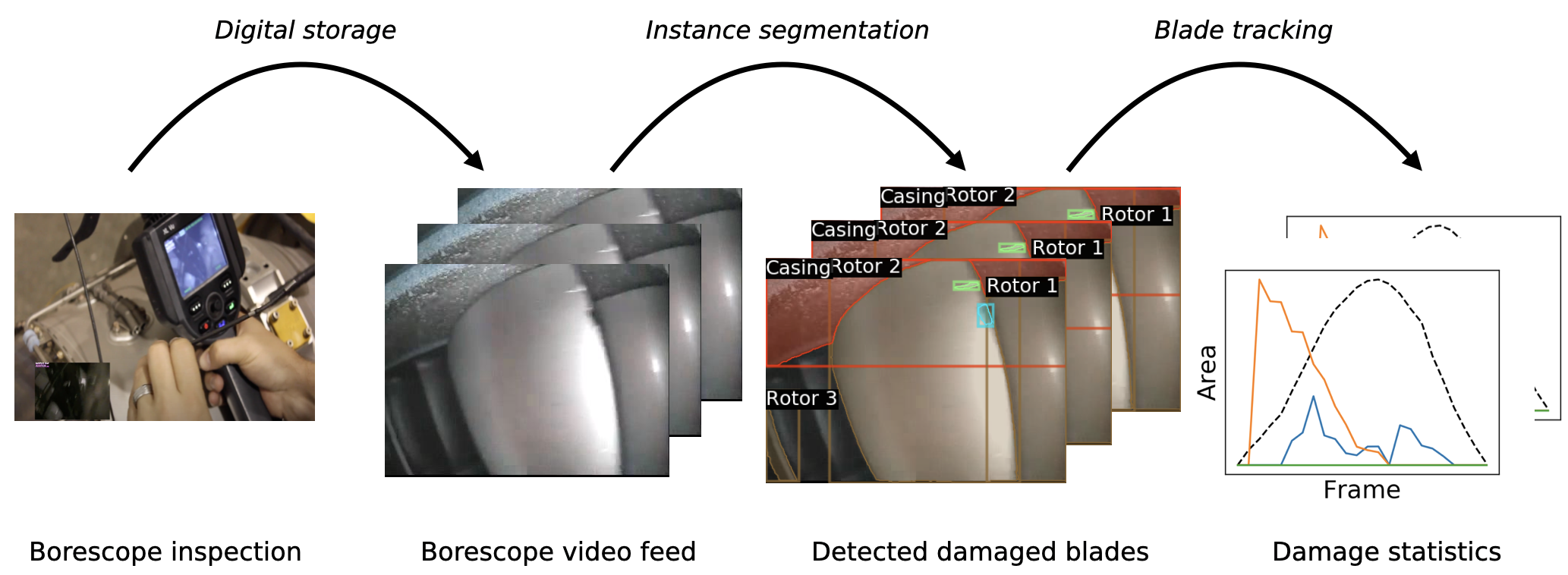
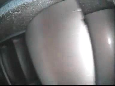
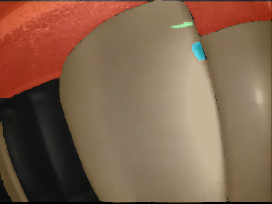
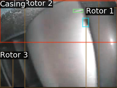
The aim of the work presented in this paper is to develop an automatic workflow for assessing damage on bladed gas turbine components via analysis of video feeds collected from borescope inspections (see Figure 1). The advantages of an automatic framework include the removal of human biases, a faster decision process, possible gains in accuracy, and—in the face of uncertainty—the ability to quantify this uncertainty via confidence scores. In this workflow, video feeds collected from borescope inspections are stored and input to a bespoke neural network. The structure of the component in the video is deduced via an instance segmentation framework based on deep learning. In instance segmentation, each object within a video frame is detected, classified and localised with a bounding box surrounding the object. Within this bounding box, the object is identified by a mask that highlights relevant pixels. Figure 2 illustrates the differences between three common image segmentation tasks in computer vision, namely semantic segmentation (where each pixel is classified), object detection (where bounding boxes are deduced for each object and classified) and instance segmentation. In literature, neural networks have been deployed to perform semantic segmentation on images collected from borescopes to detect the presence of cracks [27] and spallation [3] on turbine blades. Our work extends and differs from these papers in two main aspects: we aim to (i) classify multiple types of damage, and (ii) deduce the structure of the scene in the borescope video feed by separately identifying multiple blades—noting that, in semantic segmentation, no distinction is made between different instances of the same type of objects. Thus, semantically segmented images are unable to tell us which blade a detected damage region belongs to. By using an instance segmentation framework instead, it is possible to design a procedure to track rotor blades across a sequence of frames as the row is rotated in the captured video during a borescope inspection process. As a result, damage statistics can be extracted for individual blades as they pass through the view of the borescope.

Figure 1: Overview of automatic borescope damage assessment workflow. The borescope inspection image on the left is from https://youtu.be/gChfhRZ\_pN0.

(a) Original image

(b) Semantic segmentation

(c) Object detection

(d) Instance segmentation

Figure 2: Illustrating different segmentation tasks in computer vision. In the segmentation results, red denotes casing, brown denotes rotor, green denotes surface damage and blue denotes material separation.

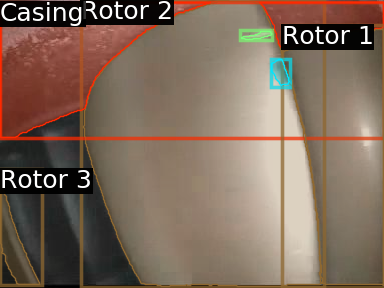
The rest of this paper is structured as follows. In Section 2, we provide an overview of the computational methods used in this work, including a review of methods for instance segmentation and a modular description of the neural network used in our study. In addition, we propose approaches to track detected rotor blades across a sequence of frames, enabling us to create summary statistics of the types and extent of damage found on individual blades. In Section 3, results obtained from the workflow on two example borescope videos are discussed with details of the methods used to assess segmentation quality.

2 Methodology

2.1 Instance segmentation with Mask Region-based Convolutional Neural Networks

Instance segmentation is an active area of research within the computer vision community. Nearly all approaches within this area are based on convolutional neural networks (CNNs) [16, 15]. These networks are attractive because of their ability to extract features of an image at various scales with translational invariance. Their architecture greatly reduces the number of parameters compared to a fully connected feedforward neural network, enabling greater efficiency in training. Thus, they form the basis of approaches to tackle tasks such as semantic segmentation [20] and object detection [10, 9, 26, 25]. Likewise, they are crucial components in state-of-the-art approaches in instance segmentation, including Mask Region-based Convolutional Neural Networks (Mask R-CNN) [12], DeepMask [24] and Fully Convolutional Instance Segmentation [17].

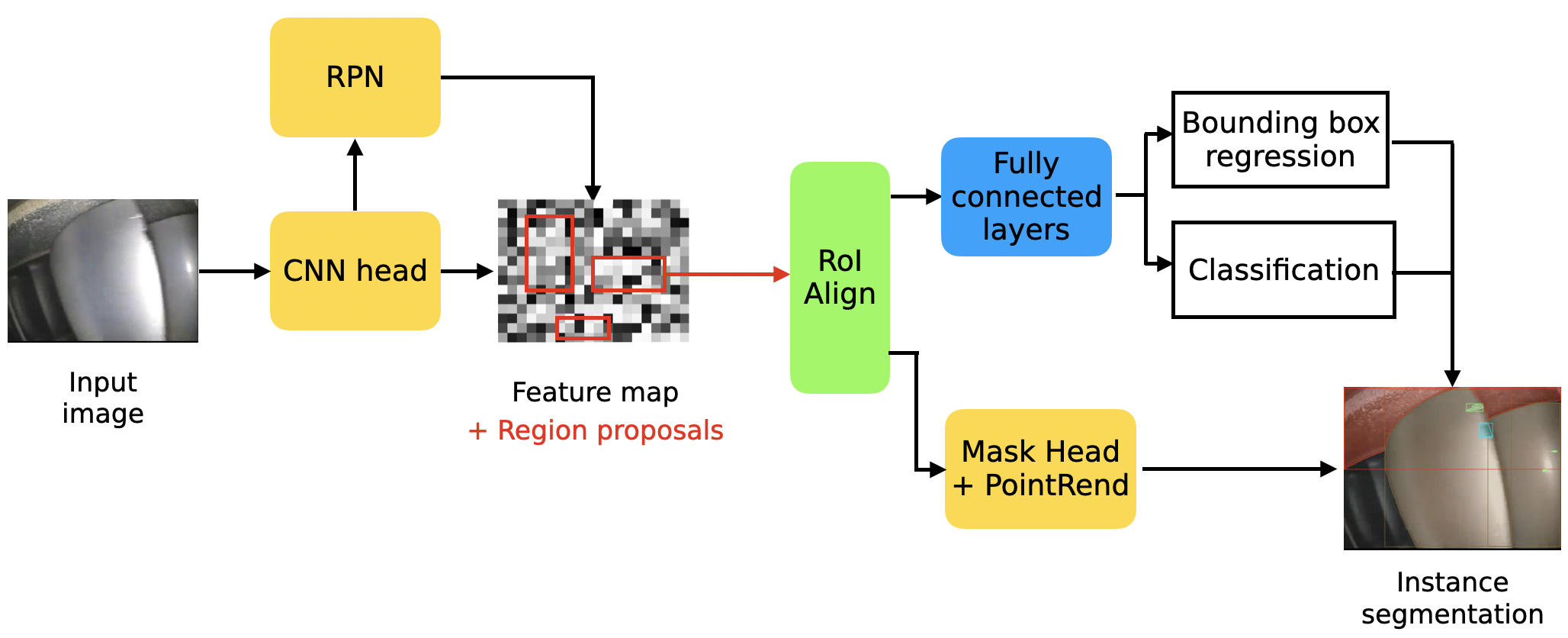
In this paper, instance segmentation on contiguous frames of borescope videos is performed by adapting the Mask R-CNN. In the following, we briefly describe the structure of this network, referring readers to the original paper [12] for further details. The first stage of the Mask R-CNN consists of a CNN head (consisting of convolutional and pooling layers) producing a feature map. This is followed by a Region Proposal Network (RPN), which is another set of convolutional layers that outputs a class prediction and bounding box coordinates for a number of anchors centered at each pixel of the feature map. Each anchor is a rectangular box of a certain aspect ratio and scale. The RPN produces a number of region proposals from anchors at different sizes, and assigns them scores indicating the confidence that an object is contained within the proposal bounding boxes. Each proposal, along with the features within the region, is properly aligned into a standard size with a method called RoI Align. Then, it is fed into a network with fully connected layers. This network outputs bounding boxes with refined coordinates that should tightly wrap around objects of interest, along with a classification of the object inside into prescribed classes. Simultaneously, the mask head takes in the region proposals and performs semantic segmentation in each region. The architecture of the entire network is shown in Figure 3 with a simplified representation.

Figure 3: Simplified schematic of the Mask R-CNN.

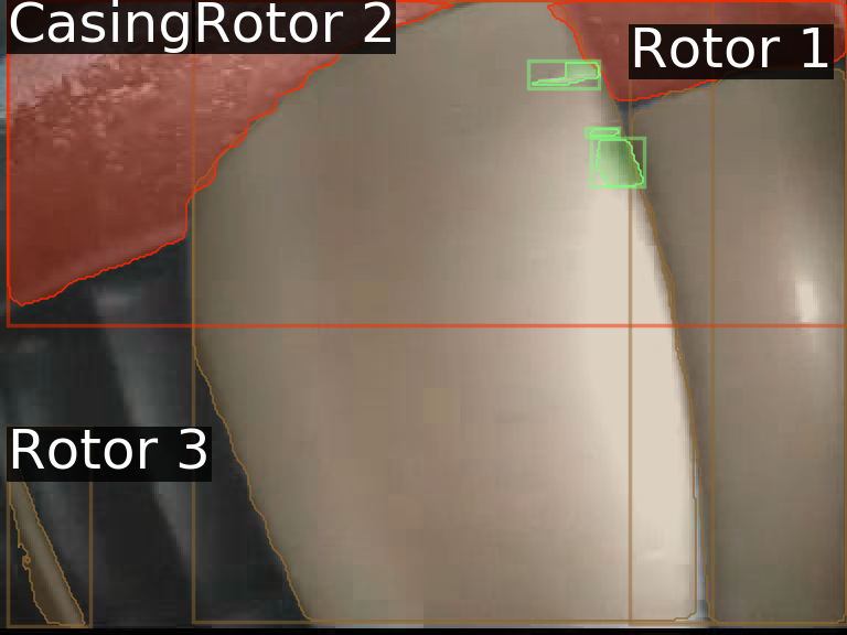
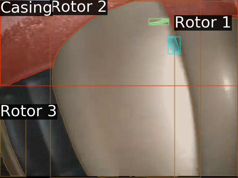
In this project, we find that, on its own, the mask head is unable to produce high quality predictions. As this network is required to operate on region proposals that can differ greatly in scale and aspect ratio within the same image, a network that can effectively segment small objects is unable to produce clean outputs for larger objects, creating undesirable artefacts such as those shown in Figure 4(a). Therefore, we incorporate the PointRend module [14] on top of Mask R-CNN to improve the segmentation accuracy of the mask head. This module performs point-based segmentation on adaptively re-sampled points on the feature map via an iterative subdivision algorithm. Having more points near the boundary of the object allows finer details of the shape to be captured, thus avoiding the aliasing phenomenon that produces the aforementioned artefacts. As seen in Figure 4(b), the artefacts are largely removed with the addition of PointRend.

(a) Without PointRend

(b) With PointRend

Figure 4: Instance segmentation result from Mask R-CNN (a) without and (b) with PointRend. Note the wavy boundary artefacts around the blades and casing in (a).

In this work, we adopt the open source software package Detectron2 [32], which provides a framework for defining, implementing, training and testing various neural network architectures for computer vision. It is based on the Python deep learning library PyTorch [23], and offers various implementations of Mask R-CNN as well as the PointRend mask head. In this work, the ResNet50-FPN architecture [18] is used for the backbone (the part of the network used for feature extraction over the entire image).

2.2 Blade tracking and calculation of damage statistics

The Mask R-CNN framework can be deployed to identify and segment objects in individual images. This enables the automatic detection of the presence of different blades in separate frames of the borescope video feed. However, in a contiguous sequence of frames, the same individual blade may be featured in different perspectives, at different positions within the frames. Depending on lighting conditions and the perspective of the borescope camera, various instances of damage may appear in some frames and disappear in others. To provide a holistic assessment of the condition of a certain blade, it is necessary to track blades across the frames they appear in. Since this information is not available from the Mask R-CNN, we design an algorithm to find correlations within a sequence of frames and identify identical blades across adjacent frames.

In Section 2.2, the procedure used to assign unique ID values to blades appearing in a sequence of frames in a video feed is described. Several assumptions are made with this algorithm, which explain the motivation behind its design. First, owing to the contiguous nature of blades moving across frames, we assume that blades do not move significantly across adjacent frames. That is, the displacement of a blade from the previous frame is below a certain threshold. In other words, we assume a high frame rate relative to the rotation speed of the blades. This motivates the approach to match the blade in the current frame to the nearest blade in the previous frame in terms of the Euclidean distance between the centres of the respective bounding boxes. For each blade in the current frame, this distance is calculated with all blades in the previous frame. If the minimum distance is below a certain user-set threshold (depending on the video), the blades can be matched and the ID copied onto the current blade. If the minimum distance is larger than the threshold, it is understood that this blade is not seen in the previous frame. Hence, a new ID is set for this blade. In the implementation, we look back to a short sequence of frames (of user-set length $L$) to protect against missing detections in certain frames. Moreover, blade detections with area smaller than a certain user-set threshold are also discarded. In frames with small projected blade areas, it is unlikely that marks of damage on the blade will be clearly visible. We note that the assumption of continuity is broken when the video contains a discontinuity, or the camera is moved too quickly. In practice, some pre-processing is necessary to prevent these possibilities, e.g. by breaking up discontinuous video segments.

Input : Instance segmentation results for each frame, distance, area and detection confidence thresholds, length of lookback $L$.

Output : Blade IDs for each blade in each frame.

1

2for each frame do

3      Mark all blades with projected area larger than area threshold and confidence score above confidence threshold as valid.

4      if first frame in the video then

5           Assign new IDs for each valid blade.

6           Continue

7          

8           end if

9          

10          for $k=1,...,L$ do

11                for each valid unmatched blade in current frame do

12                     for each valid blade $k$ frames ago do

13                          Calculate the distance between the current blade and previous blade by Euclidean distance between centres of respective bounding boxes.

14                         

15                          end for

16                         Identify blade with minimum distance.

17                          if minimum distance is smaller than distance threshold then

18                               Set ID of current blade as the ID of the previous blade.

19                              

20                               end if

21                              

22                               end for

23                              

24                               end for

25                              

26                              for each unmatched blade in current frame do

27                                    if left-leaving blades is not empty and current blade’s bounding box is on the left side of frame then

28                                         Assign ID as the last left-leaving blade.

29                                        

30                                         else if right-leaving blades is not empty and current blade’s bounding box is on the right side of frame then

31                                              Assign ID as the last right-leaving blade.

32                                             

33                                              else

34                                                   Assign new ID to blade.

35                                                   end if

36                                                  

37                                                   end for

38                                                  

39                                                   end for

40                                                  if blade from previous frame is not found in current frame then

41                                                        if center of bounding box is on the left side of frame then

42                                                             Append blade ID to left-leaving blades.

43                                                            

44                                                             else

45                                                                  Append blade ID to right-leaving blades.

46                                                                 

47                                                                  end if

48                                                                 

49                                                                  end if

Algorithm 1 Tracking blades in a video feed.

Second, we assume that the blades travel (approximately) horizontally, going from left to right or vice-versa. It is possible for the row to travel back and forth, so an unmatched blade may be a blade that has already been seen earlier in the video. To tackle this, lists of blades that have left the view on either side of the travel path are kept, and appropriately assigned to unmatched blades depending on their direction of entry. Clearly, this can be extended to the case of, e.g., vertically travelling blades, but when the borescope is non-stationary during inspection, a more sophisticated method is required.

With a system to track blades across the video, we can collate statistics about the damage on blades as seen from the various frames, identifying which blade the detected damage pixel patches in each frame belongs to. As mentioned earlier, certain marks of damage are more visible in some frames—showing a blade from certain perspectives—than others. Thus, instead of focusing on a single view, damage statistics across the whole trajectory of the blade should be recorded. In Section 3, damage is recorded for each blade as a fraction of the projected area of the blade visible in that frame. We note that this is not a unique method of quantifying and assessing damage; factors other than the area/size of the damage—such as the location of the damage—can be taken into account.

3 Results

In this section, the workflow described in this paper is demonstrated on borescope images of a high pressure compressor (HPC) collected from two videos available from YouTube (See Figure 5 and Table 1 for example images from and details of both videos.) First, further details on the implementation and deployment of the workflow are provided. Second, performance metrics for the instance segmentation are provided with discussion. Third, we describe a post-processing step to improve detection accuracy. Finally, examples of assessing damage on specific rotor blades are shown including a video visualisation.

(a) Example frame from video 1.

(b) Example frame from video 2.

Figure 5: Example images from both videos used in this work.

Table 1: Details of each borescope video used in this work.

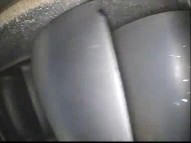
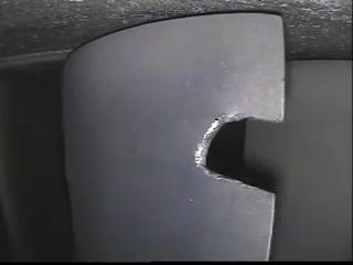
	Video 1	Video 2
Engine	Rolls-Royce RB211-535
Component	HPC fourth stage	HPC second stage
Frames per second	25	25
Number of blades visible	97 (entire row)	38

3.1 Gathering of training and testing data

Out of the 4881 video frames contained in both videos combined, 104 images are provided with manual labels via the open source Computer Vision Annotation Tool (CVAT) software. Labels are provided in the form of polygons that approximate the outline of an object (see Figure 6), and are associated with five possible classes, namely Casing, Compressor-rotor, Surface-damage, Material-separation and Material-deformation. In this dataset, Surface-damage mainly refers to scratches, but can also refer to compressor fouling, turbine sulfidation etc. Material-separation includes nicks, tears and cracks; and Material-deformation commonly refers to bends. With reference to [2], these categories are devised to broadly separate forms of damage of different nature (hence different potential impact on performance), while keeping the number of classes small.

Figure 6: Example of labelled image from CVAT.

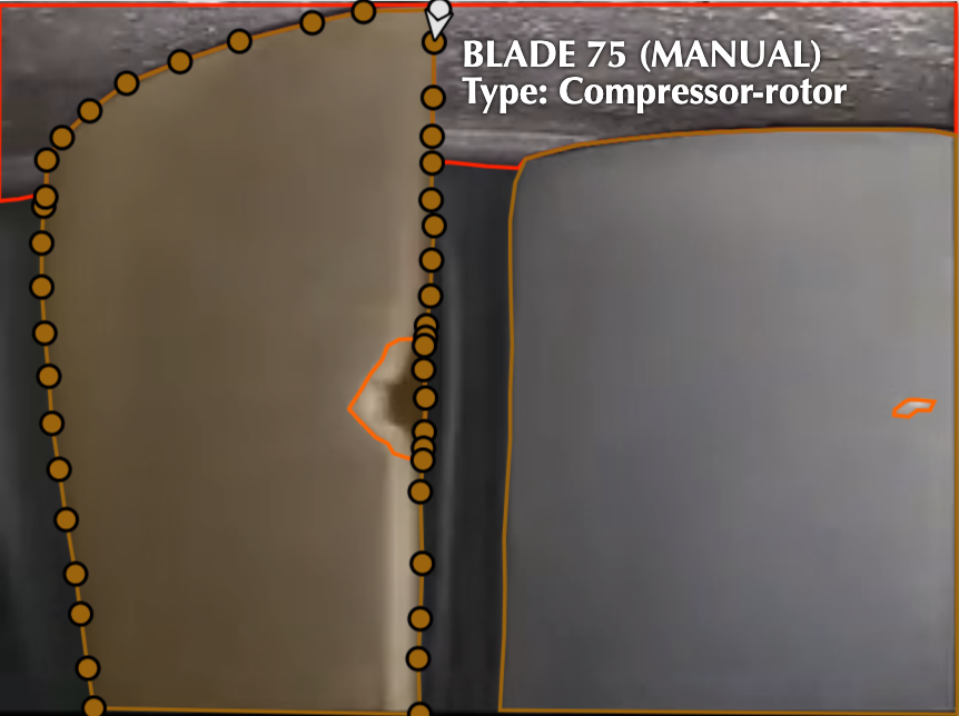
It is important to note the introduction of possible human biases in this process. First, labels may not completely tightly wrap around the object of interest. Due to the limited resolution of video frames and the presence of imaging artefacts, this is difficult to avoid, especially when concerned with small damage marks. Second, material separation and deformation damage cause the blade shape to warp. Where they occur, we interpret the blade shape as that corresponding to the original undamaged geometry. Thus, labelling blades with these types of damage involves interpolation/extrapolation of certain points, which can suffer from minor variations. Despite the above, we argue that overall, the automatic framework should mitigate the impact of possible biases compared to a fully manual procedure. For example, the system can highlight damage that may be missed in manual inspections.

3.2 Training of the neural network

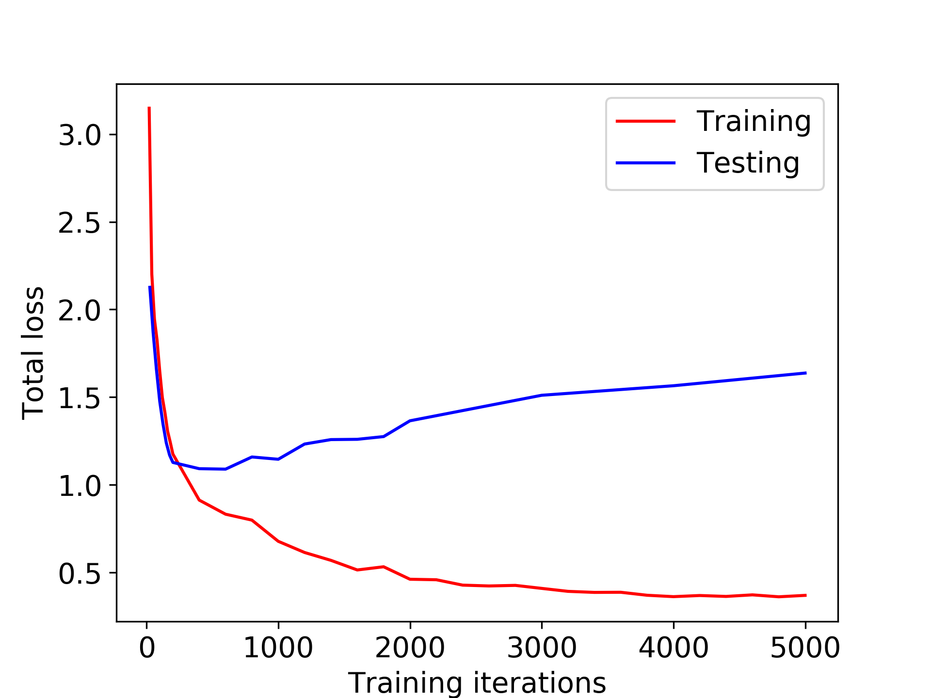
From the 104 labelled images, 89 images are used for training, and 15 for testing. Network weights are initialised from the pre-trained model for the COCO dataset [19] . The network is trained with a learning rate of 0.02, a weight decay parameter of 0.0001 and momentum of 0.9 using stochastic gradient descent (SGD). The mini-batch size is 16, distributed across 4 GPUs. The network is trained for 2000 iterations (see the next subsection for discussion of this choice). Most of the network configurations follow the defaults set in [32] according to [12] and [14], except for the anchor sizes. Due to the lower resolution of our images ($384\times 288$), and the presence of small surface damage marks, the proposal anchor sizes for the RPN are set as 16, 32, 64, 128 and 256, smaller than the default.

The multi-task loss function of the Mask R-CNN is composed of five terms,

$$L_{tot}=L_{rpn,cls}+L_{rpn,reg}+L_{cls}+L_{reg}+L_{mask}.$$ (1)

The first two terms refer to losses of the region proposals generated by the RPN. The first term $L_{rpn,cls}$ is a binary cross entropy loss over whether a region proposal contains or does not contain an object. The term $L_{rpn,reg}$ penalises discrepancies of the bounding box with ground truth bounding boxes automatically generated from the polygon labels, and is only calculated for positive region proposals, i.e. those with sufficient overlap with a ground truth box. The latter three terms refer to the mask head. The term $L_{cls}$ is a multinomial cross entropy loss, now penalising wrong classifications of the object within a bounding box. $L_{reg}$ works similarly to $L_{rpn,reg}$ but for final output bounding boxes instead of region proposals. Finally, $L_{mask}$ is the semantic segmentation loss within each positive bounding box.

We note that the number of training iterations and number of training images is small compared with common benchmark datasets for instance segmentation (e.g. COCO [19], Cityscapes [5]). However, it is shown in the following that this nevertheless results in satisfactory quality in the predictions. This is mainly because of the similarity of the frames in a single video feed. In practice, if the scope of the workflow were to be increased by sourcing training data from borescope inspections of more distinct components, the size of the training set and duration of training would need to be increased appropriately.

3.3 Results on testing data

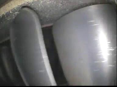
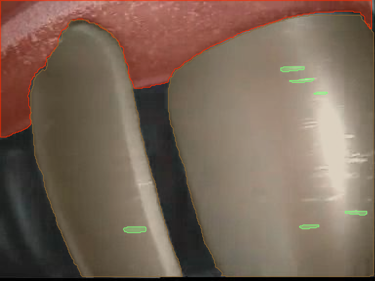
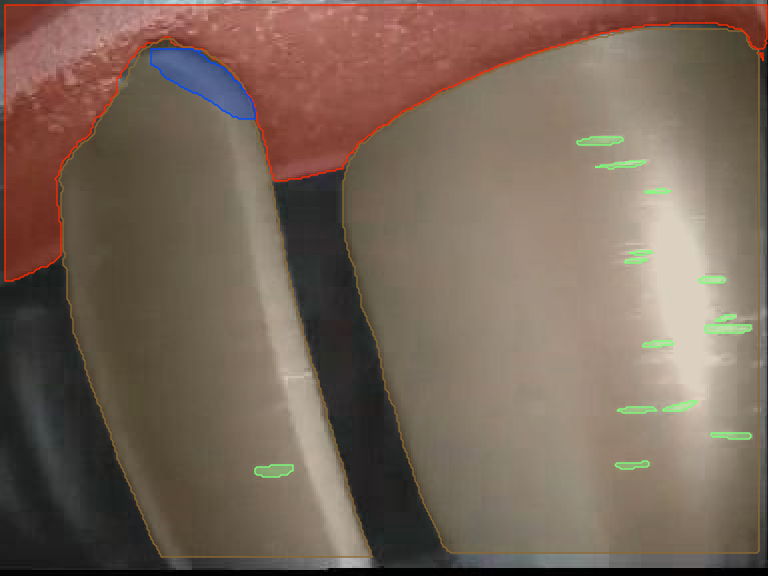
In Figure 7(a), the total loss (1) is plotted against the number of training iterations. Although the loss on the training data continues decreasing as the number of iterations increase, the loss on the testing data increases after about 200 iterations. This suggests that the model is overfitting past 200 iterations. However, it is observed that detection quality is improved when comparing the network at a later stage to that at an earlier stage of training, even on unseen testing images. For example, Figure 8 shows a testing image and the corresponding network predictions after 500 and 2000 training iterations respectively. This figure shows that the network after 500 iterations tends to skip the identification of certain damage marks—e.g. some surface damage on rotor 46 and the tip bend near the leading edge of rotor 47. Therefore, the testing loss is not an adequate metric for judging the quality of the network in this case. A possible cause of this is that the loss does not penalise missing detections severely enough—e.g. the mask segmentation loss $L_{mask}$ is only defined on valid region proposals.

Thus, we propose to evaluate the network using two different metrics. They are based on comparing predicted masks with masks from the ground truth (manually labelled images) using the intersection over union (IoU) metric. For two masks $A$ and $B$, their IoU is

$$IoU=\frac{\text{Area}(A\cap B)}{\text{Area}(A\cup B)},$$ (2)

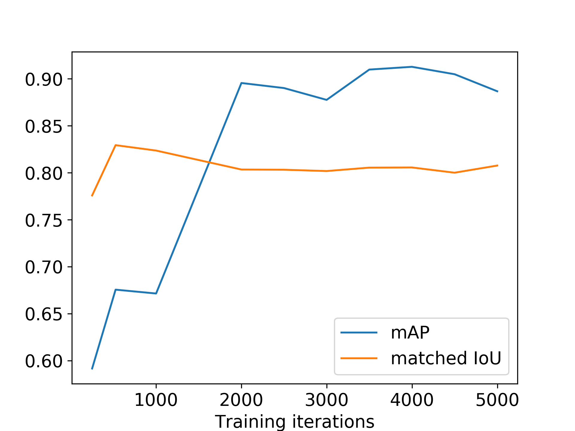
which is a measure of how much overlap the masks have. The mean average precision (mAP) is a common metric used in computer vision literature to evaluate instance segmentation networks. It is evaluated using the steps detailed in Section 3.3 (also see [22]) at a certain IoU threshold that we set at 0.5. This is also known as AP₅₀ in literature [12]. It is a measure of the proportion of masks that correctly predict objects in the ground truth of an image, in terms of both the class and a minimum IoU. In addition to this metric, we devise a similar metric—the matched IoU— that measures the average IoU of True mask predictions with their assigned ground truth masks obtained from Section 3.3 for each class. This is subsequently averaged across all classes. This metric measures the quality of matched masks in addition to their well-matching with ground truth masks, since the calculation of areas is a crucial part of our results. In Figure 7(b), we have plotted these two metrics averaged across the images in the testing data, evaluated for the network trained at different numbers of training iterations. From this figure, it is clear that the network performs better from 2000 iterations onwards. While the matched IoU stays relatively constant, the number of missing detections is drastically reduced as we train the network, raising the mAP score.

(a)

(b)

Figure 7: (a) Training and testing losses, and (b) mean average precision (mAP) and mean matched IoU on testing data with respect to training iterations.

Input : Masks and associated class predictions and ground truth, IoU threshold value between 0 and 1.

Output : mAP value.

1 for each class do

2      List all predicted masks of a certain class, ordered in descending order of prediction confidence.

3      for each predicted mask in descending confidence do

4           if no unassigned ground truth mask of the same class exists then

5                Mark this prediction as False.

6               

7                end if

8               Find the unassigned ground truth mask of the same class that has the highest IoU with the prediction.

9                if this IoU $>$ IoU threshold then

10                     Mark this prediction as True.

11                     Mark this ground truth mask as assigned.

12                    

13                     end if

14                    else

15                          Mark this prediction as False.

16                         

17                          end if

18                         

19                          end for

20                         Set $FN=$ number of unassigned ground truth masks.

21                         

22                         for each predicted mask in descending confidence do

23                               Calculate $\tilde{P}=$ the number of True predictions so far divided by the number of predictions so far.

24                               Calculate $R=$ the number of True predictions so far divided by (the total number of True predictions + $FN$).

25                              

26                               end for

27                              Associate each $\tilde{P}$ with the corresponding $R$ to form $\tilde{P}(R)$, the precision-recall curve.

28                               Calculate $P(R)=\text{max}_{R^{\prime}\geq R}\tilde{P}(R^{\prime})$, the interpolated precision-recall curve.

29                               Calculate $AP=\int_{0}^{1}P(R)dR$.

30                               end for

Calculate $mAP=$ the mean of $AP$ across all classes.

Algorithm 2 Calculating mAP for an image.

(a) Original image

(b) Segmentation after 500 iterations

(c) Segmentation after 2000 iterations

Figure 8: Segmentation results for a frame showing rotors 46 and 47 after 500 and 2000 training iterations. Note that this frame is not in the training data.

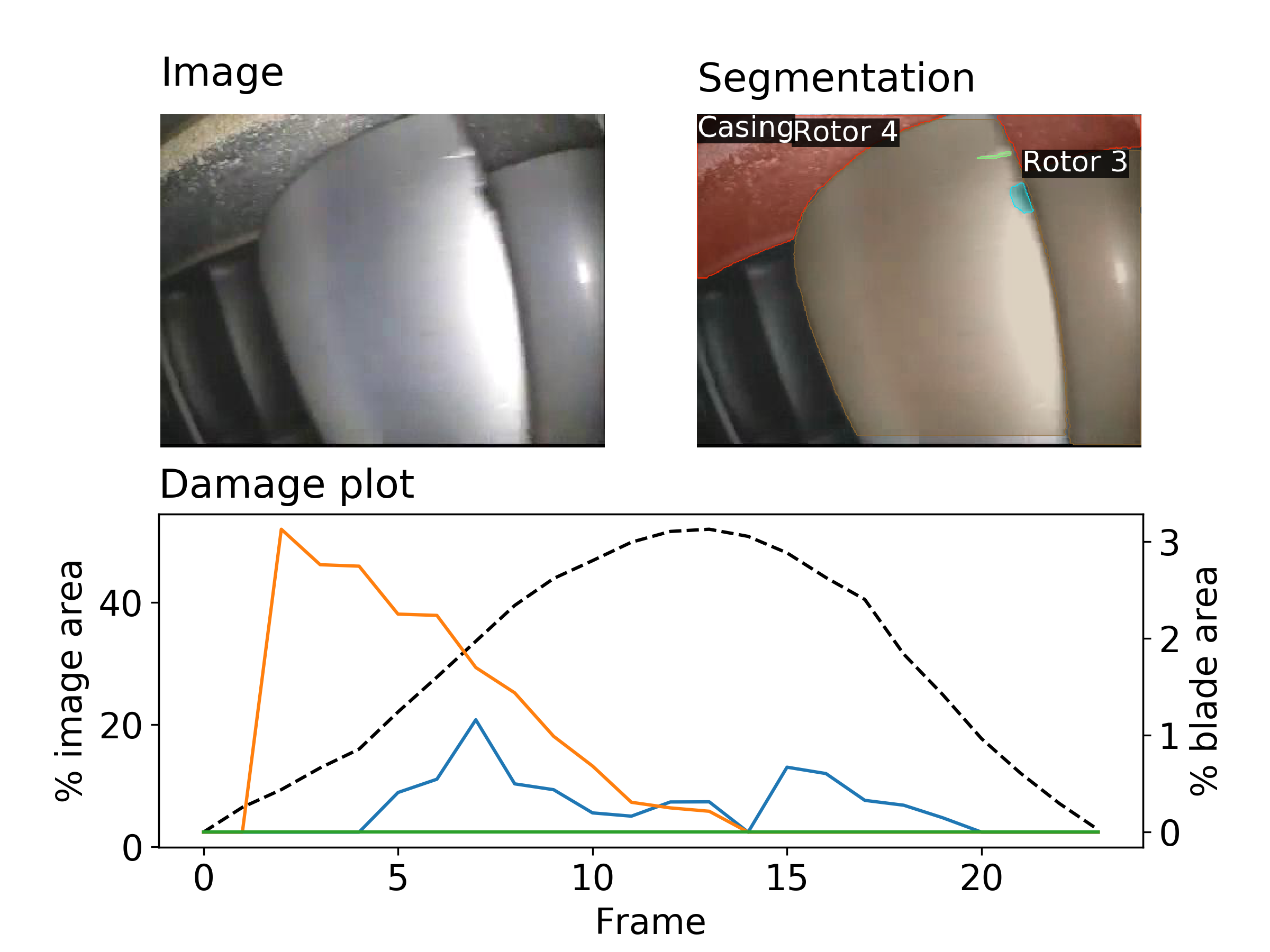
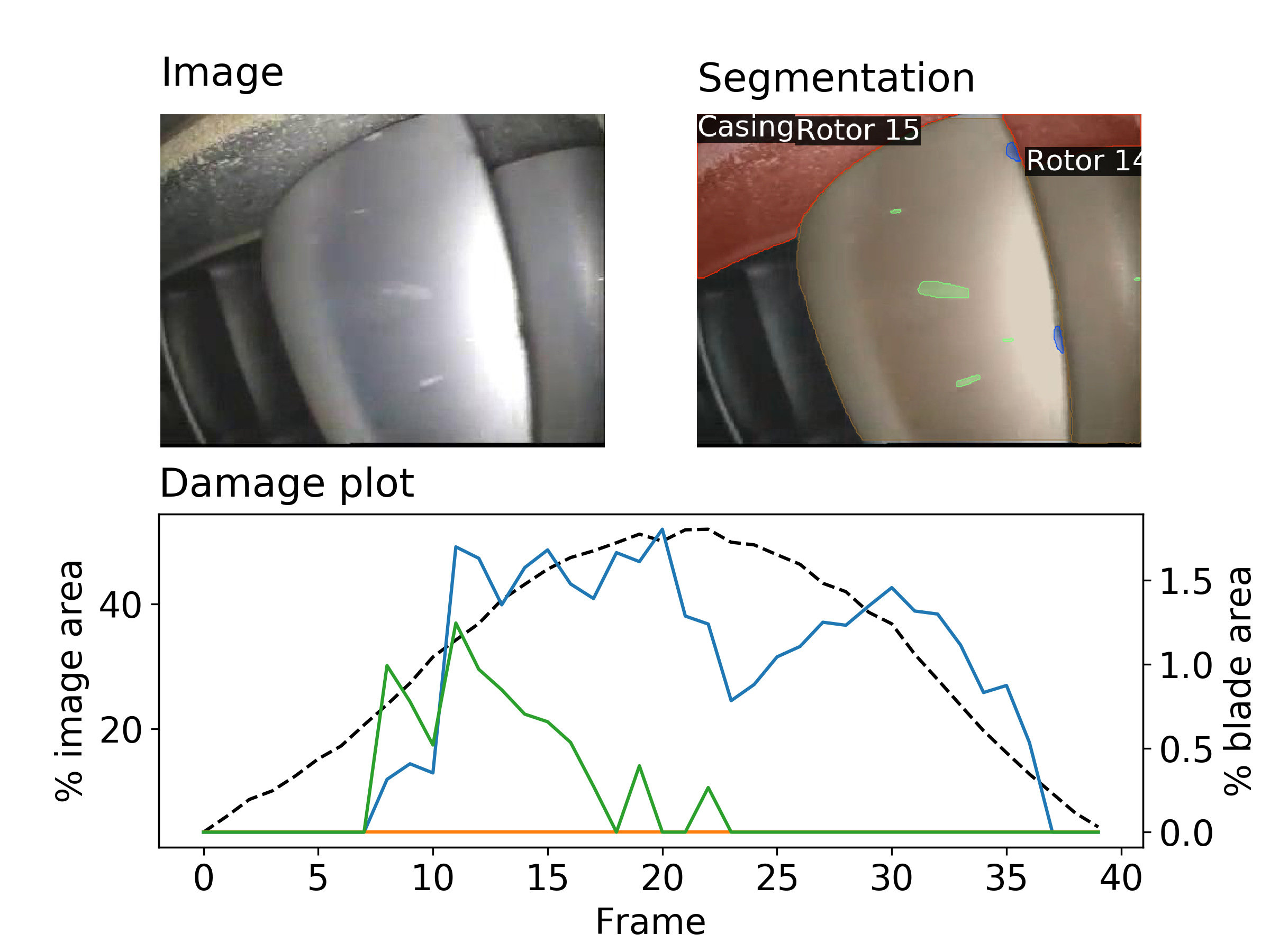
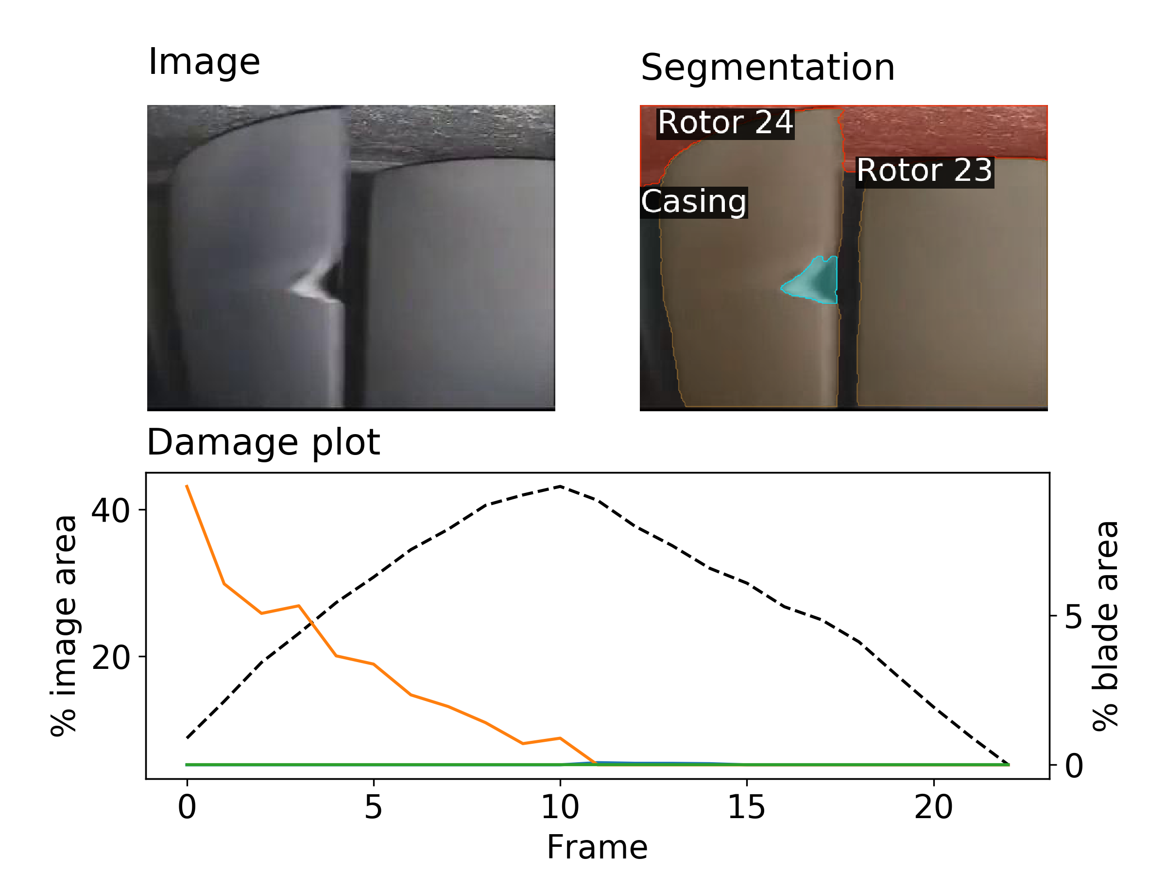
Having obtained the segmentation of each frame in the video, Section 2.2 is applied to correlate the masks across adjacent frames and assign unique IDs to each rotor found within the video sequence. Then, the projected areas of the rotors shown in the images, along with the associated area of damage present on the blades, are calculated by counting the pixels in their masks. For each rotor, it is possible to plot a time series graph, showing the amount of damage present on each blade relative to the blade projected area as the blade emerges into and then leaves the camera view. In Figures 9, 10 and 11, we show three example time series plots of the detected damage on rotors. In all three plots, the black dashed line shows the detected rotor area as a fraction of image area, and the coloured solid lines show different types of damage as a fraction of blade area; the blue line shows surface damage, the orange line material separation and green line material deformation. As the rotors travel across the camera view, the extent of detected damage varies. Therefore, a thorough assessment of rotor damage should take into account the full time series.

Figure 9: Example image, corresponding segmentation result and damage time series plot for Rotor 4, video 1.

Figure 10: Example image, corresponding segmentation result and damage time series plot for Rotor 15, video 1.

Figure 11: Example image, corresponding segmentation result and damage time series plot for Rotor 24, video 2.

3.4 Post-processing to identify surface damage

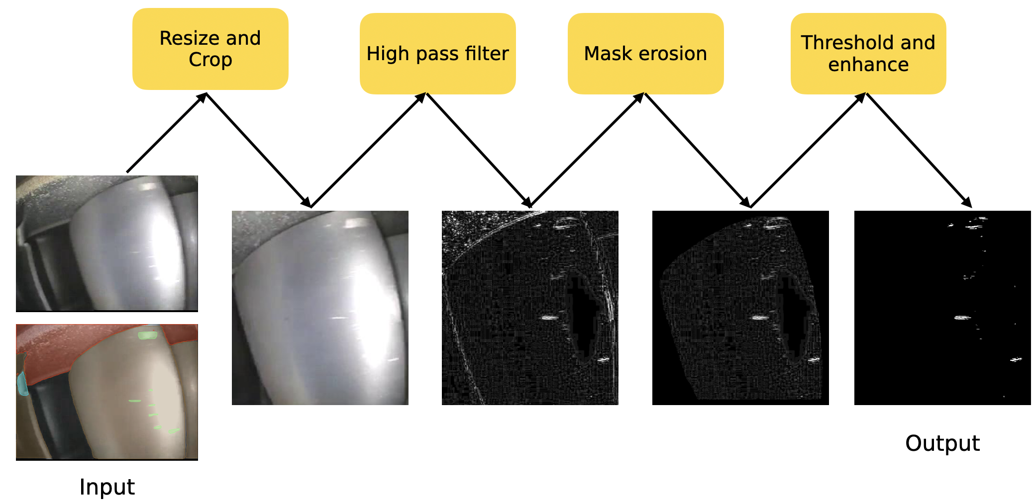
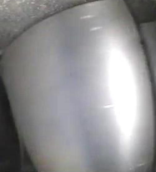
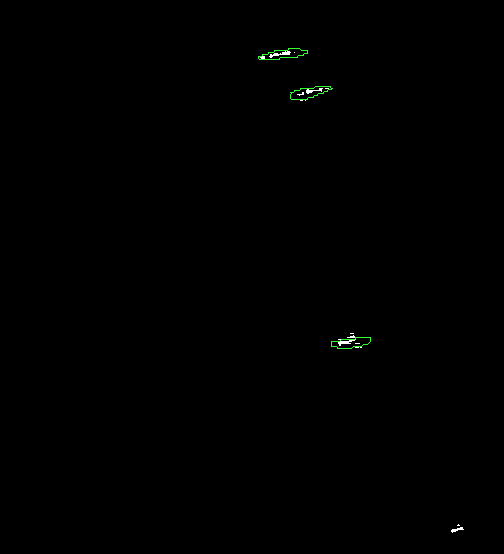
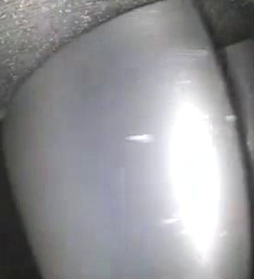
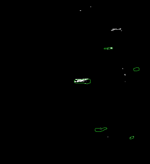
At each frame, the Mask R-CNN needs to detect and mask objects at a wide range of scales. In particular, while larger objects with clear outlines such as blades are more easily detected, smaller patches indicating surface damage on blades are more challenging. In addition, small scratches are difficult to identify through manual inspection of borescope images, which affects the labelling process that generates the training data. Therefore, surface scratches may be missed by the network occasionally. To address this, we suggest the addition of a post-processing step to check the network predictions against filtered images highlighting small scale features. An illustration of this workflow is shown in Figure 13, and consists of the following steps:

1. Resize and crop to isolate an individual blade from a frame, using network predictions to find the bounding box of the blade.

2. Apply a high-pass filter to the image within the box. Let $\mathbf{I}$ be the $H\times W$ matrix of grayscale pixel brightness intensities, where $H$ and $W$ are the height and width of the bounding box respectively. The output $\mathbf{I}_{h}$ is given by

   $$\mathbf{I}_{h}=[\mathbf{I}-\mathbf{I}*\mathbf{G}_{\sigma}]_{+},$$ (3)

   where $\mathbf{G}_{\sigma}$ is the isotropic Gaussian smoothing kernel with standard deviation $\sigma$ [6, Ch. 9.12.6], $*$ is the (discrete) convolution operator and $[\cdot]_{+}$ sets all negative elements of the argument to zero.

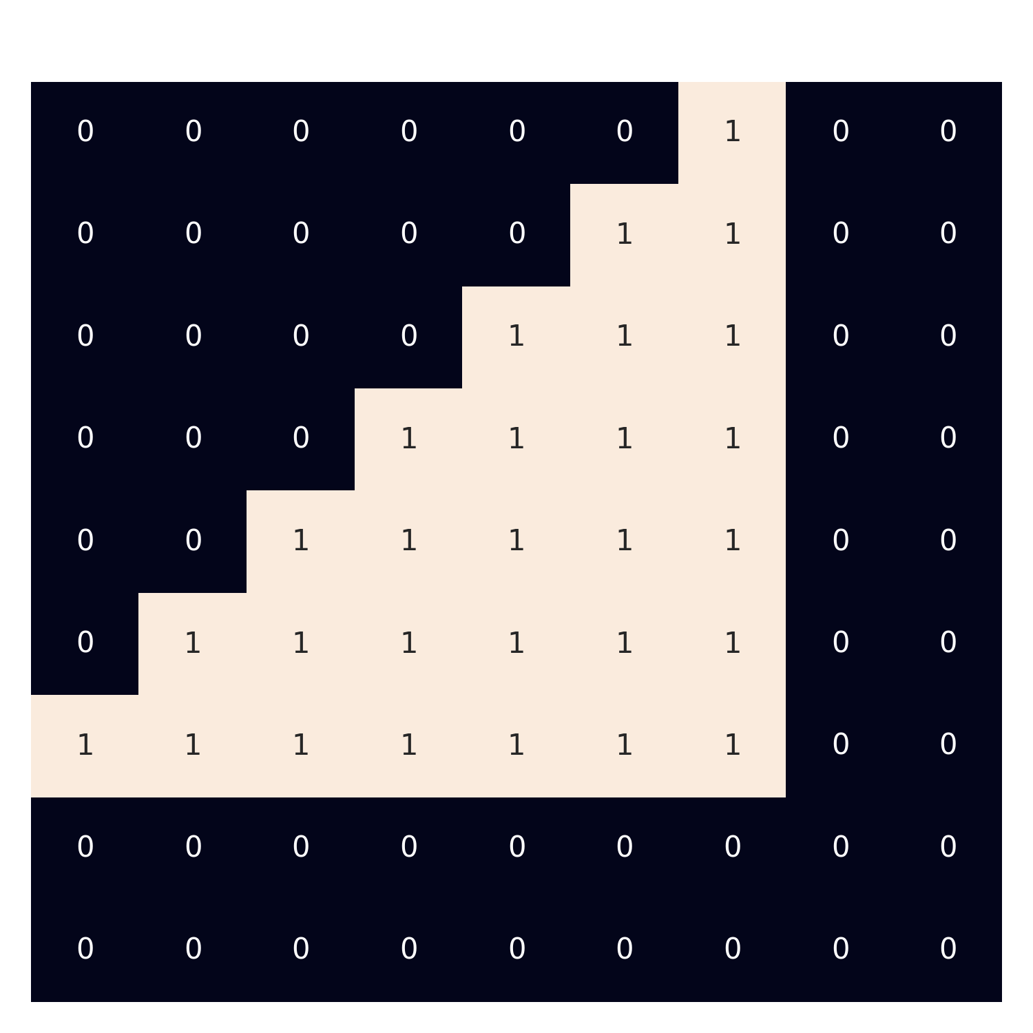
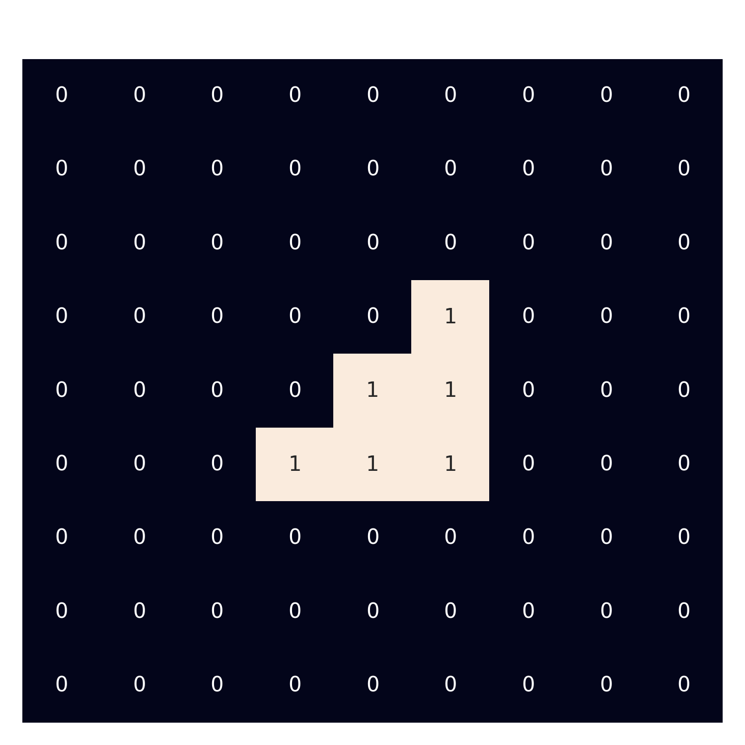
3. Mask erosion: We apply a mask to the output of the high-pass filter which sets the elements outside of the mask to zero. The mask used is a morphologically eroded version of the blade mask generated by Mask R-CNN within the bounding box. That is, the expanse of the mask is shrunk at the boundary in the normal direction (see Figure 12). This operation removes the highlight at the blade edges which is picked up by the high-pass filter.

4. Finally, we apply a threshold and enhance operation to remove pixels with low intensities, and enhance the contrast of the final output.

Using the steps above, small features and discontinuities over the blade are demarcated.

(a) Before erosion

(b) After erosion

Figure 12: Demonstrating the morphological erosion operator on an example binary array.

Figure 13: Example procedure to generate filtered images that highlight small features on blades leveraging network predictions. Note that enhancing is applied for the final three images for exposition purposes.

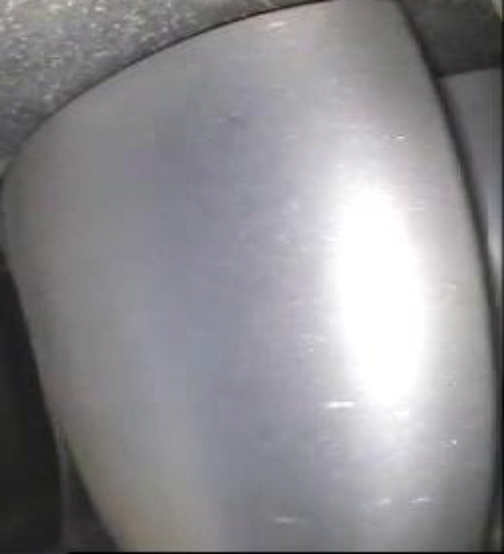
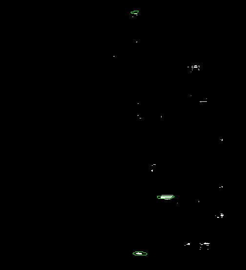
In Figure 14, these steps are demonstrated on three distinct blades in frames with maximum projected area. It can be seen that the network does not identify all surface scratches, which may even be difficult to identify manually. The high-pass filtering procedure removes the glare of the blade’s reflection and shows the presence of small irregularities on the blade surface. It should be noted that this procedure has certain limitations—such as the susceptibility to noise artefacts, the necessity to manually tune the size of the filters, and the inability to distinguish between different types of damage.

Figure 14: Original images (top) and post-processed images (bottom) showing three different blades with surface damage. White pixels indicate the intensity post-filtering, and green contours denote masks from Mask R-CNN.

3.5 Analysis of damage around blade row

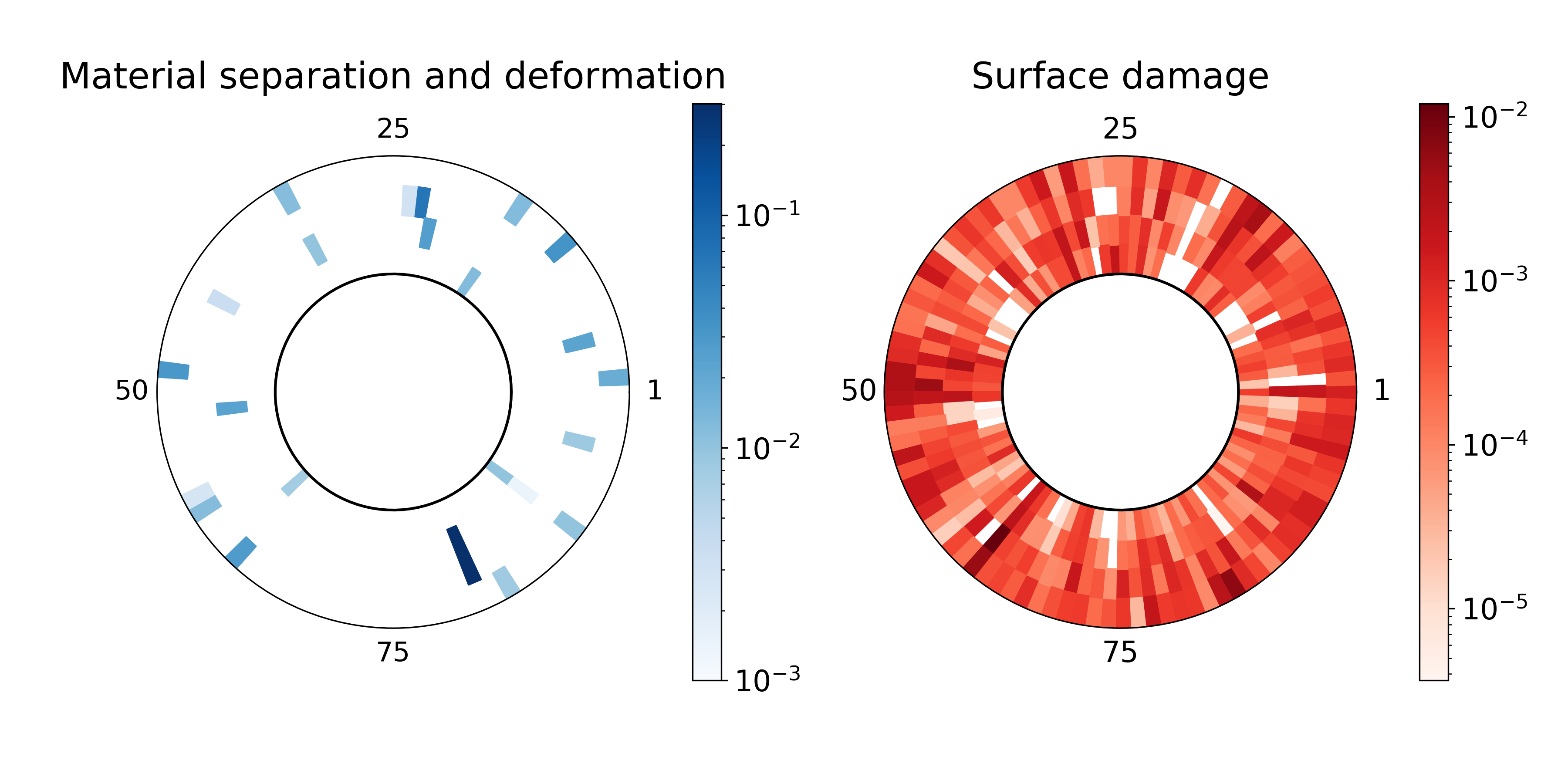
In the following, we detail the damage found around the rotor row in video 1, where the full blade row is shown. In Figure 15, the damage extent on each blade around the rotor disk is summarised and illustrated. For material separation and deformation damage, the extent is calculated from its area in the frame in which it has the maximum projected area; for surface damage, the extent is considered by averaging across all frames, since surface damage is usually made up of a number of small scratches, with only a subset of all surface damage patches on a certain blade visible in a particular frame. In both plots, the amounts of damage are plotted separately for four spanwise regions as a fraction of the entire projected rotor area. These plots reveal important insights about the detected damage. For example, rotor imbalances can be detected when severe separation damage is present in one localised region around the row.

We summarise the output of the entire workflow with an animation accessible at https://youtu.be/nUU-1mpvIpM. In this video, network prediction labels are visualised along with damage summary plots and a hypothetical performance impact value $\Delta f$, which is a function of the damage types and extent found on each rotor. Provided with hardware enabling fast predictions from the network, this workflow can be deployed in real time during borescope inspections for quick engine sentencing.

Figure 15: Plot of types of damage around a blade row. In both plots, color denotes the extent of damage as a fraction of rotor area, split across four spanwise regions. Spanwise position of the damage is shown with the radial coordinate, and the azimuthal coordinate denotes the rotor number.

4 Conclusions and future work

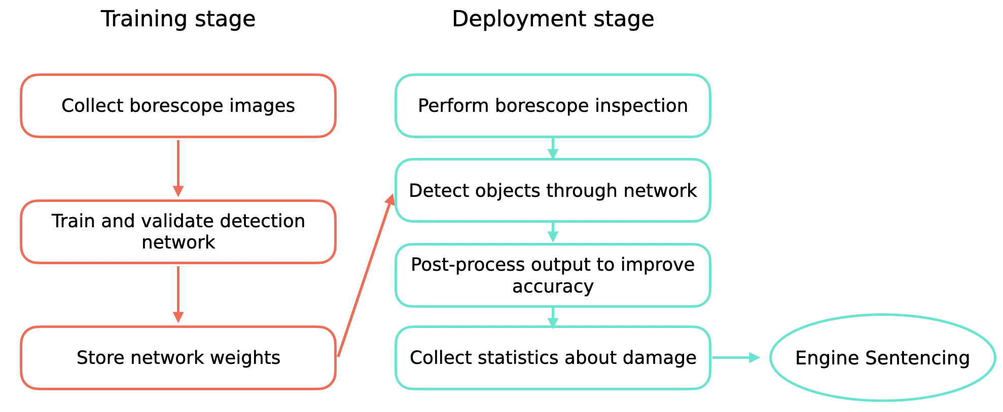
Using methods from computer vision, we show that it is possible to detect damage present on blades via videos collected from borescope inspections. Coupled with algorithms for blade tracking, this enables an automatic workflow that collects statistics about the types and extent of damage found on rotor blades. To summarise, the steps for training and deploying the automatic borescope inspection framework in practice are outlined in Figure 16.

Figure 16: Summary of the training and deployment of the automatic borescope inspection framework.

To take this work further, we need to convert the collected damage statistics over several frames to a full assessment of the damaged geometry of a blade. This involves the mapping of detected damage in 2D to a 3D model of a blade in CAD representation. The 3D blade models serve as digital twins that are amenable to aerodynamic analysis to assess the implications of the damage. For example, in [30, 31], the authors propose a method to measure a metric distance of a geometry from a collection of blades that are known to adhere to performance and safety standards—called a blade envelope. Integrating the present framework with the workflow in [30, 31], we envision that our system can serve as a component in a real-time assessment and recommendation system to aid inspectors in engine sentencing and engineers in designing robust bladed components.

References

- [1] Rafael R. Adamczuk and Joerg R. Seume. Early Assessment of Defects and Damage in Jet Engines. Procedia CIRP, 11:328–333, January 2013.
- [2] Jonas Aust and Dirk Pons. Taxonomy of Gas Turbine Blade Defects. Aerospace, 6(5):58, May 2019.
- [3] Xiao Bian, Ser Nam Lim, and Ning Zhou. Multiscale fully convolutional network with application to industrial inspection. In 2016 IEEE Winter Conference on Applications of Computer Vision (WACV), pages 1–8, Lake Placid, NY, USA, March 2016. IEEE.
- [4] Tim J Carter. Common failures in gas turbine blades. Engineering Failure Analysis, 12(2):237–247, April 2005.
- [5] Marius Cordts, Mohamed Omran, Sebastian Ramos, Timo Rehfeld, Markus Enzweiler, Rodrigo Benenson, Uwe Franke, Stefan Roth, and Bernt Schiele. The Cityscapes Dataset for Semantic Urban Scene Understanding. In 2016 IEEE Conference on Computer Vision and Pattern Recognition (CVPR), pages 3213–3223, Las Vegas, NV, USA, June 2016. IEEE.
- [6] Arcangelo Distante and Cosimo Distante. Image Enhancement Techniques. In Arcangelo Distante and Cosimo Distante, editors, Handbook of Image Processing and Computer Vision: Volume 1: From Energy to Image, pages 387–484. Springer International Publishing, Cham, 2020.
- [7] Colin G Drury and Jean Watson. Human Factors Good Practices In Borescope Inspection. Technical report, Federal Aviation Administration, May 2001.
- [8] Federal Aviation Administration. Aviation Maintenance Technician Handbook - General (FAA Handbooks). Aviation Supplies and Academics, Inc., March 2013.
- [9] Ross Girshick. Fast R-CNN. In Proceedings of the 2015 IEEE International Conference on Computer Vision (ICCV), ICCV ’15, pages 1440–1448, USA, December 2015. IEEE Computer Society.
- [10] Ross Girshick, Jeff Donahue, Trevor Darrell, and Jitendra Malik. Rich Feature Hierarchies for Accurate Object Detection and Semantic Segmentation. In 2014 IEEE Conference on Computer Vision and Pattern Recognition, pages 580–587, Columbus, OH, USA, June 2014. IEEE.
- [11] Benjamin Hanschke, Thomas Klauke, and Arnold Kühhorn. The Effect of Foreign Object Damage on Compressor Blade High Cycle Fatigue Strength, volume Volume 7A: Structures and Dynamics of Turbo Expo: Power for Land, Sea, and Air. 2017. _eprint: https://asmedigitalcollection.asme.org/GT/proceedings-pdf/GT2017/50923/V07AT31A005/2434362/v07at31a005-gt2017-63599.pdf.
- [12] K. He, G. Gkioxari, P. Dollár, and R. Girshick. Mask R-CNN. In 2017 IEEE International Conference on Computer Vision (ICCV), pages 2980–2988, October 2017. ISSN: 2380-7504.
- [13] Nqobile Khani, Clara Segovia, Rukshan Navaratne, Vishal Sethi, Riti Singh, and Pericles Pilidis. Towards Development of a Diagnostic and Prognostic Tool for Civil Aero-Engine Component Degradation. In GTINDIA2012, pages 803–814, ASME 2012 Gas Turbine India Conference, December 2012.
- [14] Alexander Kirillov, Yuxin Wu, Kaiming He, and Ross Girshick. PointRend: Image Segmentation As Rendering. In 2020 IEEE/CVF Conference on Computer Vision and Pattern Recognition (CVPR), pages 9796–9805, Seattle, WA, USA, June 2020. IEEE.
- [15] Alex Krizhevsky, Ilya Sutskever, and Geoffrey E. Hinton. ImageNet Classification with Deep Convolutional Neural Networks. Advances in Neural Information Processing Systems, 25:1097–1105, 2012.
- [16] Y. Lecun, L. Bottou, Y. Bengio, and P. Haffner. Gradient-based learning applied to document recognition. Proceedings of the IEEE, 86(11):2278–2324, November 1998.
- [17] Y. Li, H. Qi, J. Dai, X. Ji, and Y. Wei. Fully Convolutional Instance-Aware Semantic Segmentation. In 2017 IEEE Conference on Computer Vision and Pattern Recognition (CVPR), pages 4438–4446, July 2017. ISSN: 1063-6919.
- [18] Tsung-Yi Lin, Piotr Dollar, Ross Girshick, Kaiming He, Bharath Hariharan, and Serge Belongie. Feature Pyramid Networks for Object Detection. In 2017 IEEE Conference on Computer Vision and Pattern Recognition (CVPR), pages 936–944, Honolulu, HI, July 2017. IEEE.
- [19] Tsung-Yi Lin, Michael Maire, Serge Belongie, James Hays, Pietro Perona, Deva Ramanan, Piotr Dollár, and C. Lawrence Zitnick. Microsoft COCO: Common Objects in Context. In David Fleet, Tomas Pajdla, Bernt Schiele, and Tinne Tuytelaars, editors, Computer Vision – ECCV 2014, Lecture Notes in Computer Science, pages 740–755, Cham, 2014. Springer International Publishing.
- [20] J. Long, E. Shelhamer, and T. Darrell. Fully convolutional networks for semantic segmentation. In 2015 IEEE Conference on Computer Vision and Pattern Recognition (CVPR), pages 3431–3440, June 2015. ISSN: 1063-6919.
- [21] Cyrus B. Meher-Homji and George Gabriles. Gas Turbine Blade Failures - Causes, Avoidance, And Troubleshooting. Technical report, Texas A&M University. Turbomachinery Laboratories, 1998.
- [22] R. Padilla, S. L. Netto, and E. A. B. da Silva. A Survey on Performance Metrics for Object-Detection Algorithms. In 2020 International Conference on Systems, Signals and Image Processing (IWSSIP), pages 237–242, July 2020. ISSN: 2157-8702.
- [23] Adam Paszke, Sam Gross, Francisco Massa, Adam Lerer, James Bradbury, Gregory Chanan, Trevor Killeen, Zeming Lin, Natalia Gimelshein, Luca Antiga, Alban Desmaison, Andreas Kopf, Edward Yang, Zachary DeVito, Martin Raison, Alykhan Tejani, Sasank Chilamkurthy, Benoit Steiner, Lu Fang, Junjie Bai, and Soumith Chintala. PyTorch: An Imperative Style, High-Performance Deep Learning Library. In H. Wallach, H. Larochelle, A. Beygelzimer, F. d\textquotesingle Alché-Buc, E. Fox, and R. Garnett, editors, Advances in Neural Information Processing Systems 32, pages 8024–8035. Curran Associates, Inc., 2019.
- [24] Pedro O. Pinheiro, Ronan Collobert, and Piotr Dollár. Learning to segment object candidates. In Proceedings of the 28th International Conference on Neural Information Processing Systems - Volume 2, NIPS’15, pages 1990–1998, Montreal, Canada, December 2015. MIT Press.
- [25] J. Redmon, S. Divvala, R. Girshick, and A. Farhadi. You Only Look Once: Unified, Real-Time Object Detection. In 2016 IEEE Conference on Computer Vision and Pattern Recognition (CVPR), pages 779–788, June 2016. ISSN: 1063-6919.
- [26] Shaoqing Ren, Kaiming He, Ross Girshick, and Jian Sun. Faster R-CNN: Towards Real-Time Object Detection with Region Proposal Networks. IEEE Transactions on Pattern Analysis and Machine Intelligence, 39(6):1137–1149, June 2017.
- [27] Zejiang Shen, Xili Wan, Feng Ye, Xinjie Guan, and Shuwen Liu. Deep Learning based Framework for Automatic Damage Detection in Aircraft Engine Borescope Inspection. In 2019 International Conference on Computing, Networking and Communications (ICNC), pages 1005–1010, Honolulu, HI, USA, February 2019. IEEE.
- [28] Joseph Tanner and Mark Bailey. Method and system for automated repair design of damaged blades of a compressor or turbine. U.S. Patent US20050033555A1, February 2005.
- [29] J. V. Taylor, B. Conduit, A. Dickens, C. Hall, M. Hillel, and R. J. Miller. Predicting the Operability of Damaged Compressors Using Machine Learning. Journal of Turbomachinery, 142(051010), April 2020.
- [30] Chun Yui Wong, Pranay Seshadri, Ashley Scillitoe, Andrew B. Duncan, and Geoffrey Parks. Blade Envelopes Part I: Concept and Methodology. arXiv:2011.11636 [cs, stat], January 2021. arXiv: 2011.11636.
- [31] Chun Yui Wong, Pranay Seshadri, Ashley Scillitoe, Bryn Noel Ubald, Andrew B. Duncan, and Geoffrey Parks. Blade Envelopes Part II: Multiple Objectives and Inverse Design. arXiv:2012.15579 [cs], December 2020. arXiv: 2012.15579.
- [32] Yuxin Wu, Alexander Kirillov, Francisco Massa, Wan-Yen Lo, and Ross Girshick. Detectron2. 2019.