PIntMF: Penalized Integrative Matrix Factorization method for Multi-omics data

Abstract

It is more and more common to explore the genome at diverse levels and not only at a single omic level. Through integrative statistical methods, omics data have the power to reveal new biological processes, potential biomarkers, and subgroups of a cohort. The matrix factorization (MF) is a unsupervised statistical method that allows giving a clustering of individuals, but also revealing relevant omic variables from the various blocks. Here, we present PIntMF (Penalized Integrative Matrix Factorization), a model of MF with sparsity, positivity and equality constraints.To induce sparsity in the model, we use a classical Lasso penalization on variable and individual matrices. For the matrix of samples, sparsity helps for the clustering, and normalization (matching an equality constraint) of inferred coefficients is added for a better interpretation. Besides, we add an automatic tuning of the sparsity parameters using the famous glmnet package. We also proposed three criteria to help the user to choose the number of latent variables. PIntMF was compared to other state-of-the-art integrative methods including feature selection techniques in both synthetic and real data. PIntMF succeeds in finding relevant clusters as well as variables in two types of simulated data (correlated and uncorrelated). Then, PIntMF was applied to two real datasets (Diet and cancer), and it reveals interpretable clusters linked to available clinical data. Our method outperforms the existing ones on two criteria (clustering and variable selection). We show that PIntMF is an easy, fast, and powerful tool to extract patterns and cluster samples from multi-omics data.

1 Introduction

The improvement of high-throughput biological technologies enables the production of various omics data such as genomic, transcriptomic, epigenomic, proteomic, and metabolomic data (Ritchie et al., 2015; Yugi et al., 2016). The generation of these data allows investigating biological processes in cancer or complex diseases. For example, The Cancer Genome Atlas (TCGA (Network et al., 2012)) has already produced numerous omics data for a set of 32 cancer types (Vasaikar et al., 2017). Recently, other multi-omics studies on complex diseases and single-cell data are also emergent (Rowlands et al., 2014; Bock et al., 2016; Yang, 2020).

However, integrating omics data addresses several statistical challenges, such as dealing with a large number of variables, few samples, and data heterogeneity (Bersanelli et al., 2016). Indeed, the statistical distributions of omics data are very heterogeneous. For instance, mutations can be modeled by a binary distribution, while RNAseq data can be modeled by a Negative Binomial distribution and metabolomic data by a Gaussian distribution. Besides, the omic block sizes could vary from one hundred to one billion variables. Furthermore, collecting several omics for a single sample could be difficult due to the cost and access to the biological material.

To identify potential biomarkers and new classifications in complex diseases, since the last decade, unsupervised integrative methods have been developed to analyze the multi-omics datasets (Tini et al., 2017; Huang et al., 2017; Chauvel et al., 2019; Pierre-Jean et al., 2019; Cantini et al., 2020). Blocks of omics data can be seen as matrices, and relevant information can be extracted using dimension reduction methods, particularly, matrix factorization (MF) methods (Sastry et al., 2020) and canonical correlation analysis (CCA) (Tenenhaus and Tenenhaus, 2011).

CCA methods are used to integrate multi-omics data and aim to maximize the correlation between omics under constraints (Tenenhaus and Tenenhaus, 2011; Tenenhaus et al., 2014; Rodosthenous et al., 2020).

Then, MF techniques infer two matrices when applied to a single omic data: the first one describes the structure between variables (e.g., genes, probes, regions) and the second one describes the structure between samples.

One famous MF method is the Non-Negative Matrix Factorization (NMF, (Lee and Seung, 1999)). This method implements non-negativity constraints on the two inferred matrices. NMF provides a way to explain the structure of data by providing variable profiles (dictionary for each dimension). Besides, NMF enables a classification of the samples thanks to the second matrix. The NMF is a commonly applied method used for a single omic block to identify disease subtypes in gene expression data (Burstein et al., 2015) or recently, in DNA methylation data (Reilly et al., 2019).

More recently, extensions of MF have been developed to perform integrative analysis (Mo et al., 2013; Chalise et al., 2014; Chen and Zhang, 2018). MF extensions need to infer more than two matrices: one matrix for each omic block is computed and one matrix for samples.

Matrix Factorization showed that it is a powerful technique to integrate heterogeneous data (Chauvel et al., 2019; Pierre-Jean et al., 2019; Cantini et al., 2020). In our article, we propose a Penalized Integrative Matrix Factorization method called PIntMF, to discover new patterns and a new classification of a cohort. First, to add sparsity on the first inferred matrix (corresponding to the variable blocks), we used a common regularization technique: the Least Absolute Shrinkage and Selection Operator (LASSO (Tibshirani, 1996)). Then, sparsity, non-negativity and equality constraints are added to the second matrix (corresponding to the samples) to help for the interpretability of the clustering.

Besides, we propose criteria to choose the number of latent variables and to properly initialize the algorithm.

The performance of this new unsupervised model was evaluated on both simulated and real data. We applied PIntMF on a simulated framework introduced by our group in (Pierre-Jean et al., 2019) but also on a simulated framework from (Chung and Kang, 2019). We compared our method to several existing unsupervised methods that perform both variable selection and clustering: intNMF (Chalise and Fridley, 2017), SGCCA (Tenenhaus et al., 2014), MoCluster (Meng et al., 2015), CIMLR (Ramazzotti et al., 2018), and iClusterPlus (Mo and Shen, 2018). Then, we applied the model on a murine liver dataset (Williams et al., 2016) and glioblastoma cancer data from TCGA already used in (Shen et al., 2012).

2 Method

2.1 Model description

In the following, $\mathbf{A}$ denotes a matrix, $\mathbf{a}$ a vector and $a$ a scalar. We consider $K$ matrices $\mathbf{X}_{1},\dots\mathbf{X}_{K}$ as the input of each method. Each matrix $\mathbf{X}_{k}$ is of size $n\times J_{k}$ ($n$ is the number of samples and $J_{k}$ the number of variables for the block $k$. In this article, we propose a model based on the matrix factorization method i.e.:

$$\mathbf{X}^{k}\approx\mathbf{W}\mathbf{H}^{k}$$ (1)

where $\mathbf{W}$ denotes a common basis matrix and $\mathbf{H}^{k}$ a specific coefficient matrix associated with the block $k$. $\mathbf{W}$ is of size $n\times P$ and $\mathbf{H}^{k}$ is of size $P\times J_{k}$. Therefore, the variable $P$ is the number of latent variables in the model.

To ensure identifiability and improve interpretation of the model, non-negativity and sparsity constraints are imposed on $\mathbf{W}$ (as in intNMF model described in (Chalise and Fridley, 2017)). $\mathbf{W}$ will be used to cluster samples simultaneously across the $K$ omics blocks. On $\mathbf{H}^{k}$, a sparsity constraint is imposed to perform variable selection simultaneously to the clustering of samples. The model 1 can be extended to the following optimization problem:

$$\min_{\mathbf{W},\mathbf{H}_{1},\dots,\mathbf{H}^{k}}\sum_{k=1}^{K}\|\mathbf{X}^{k}-\mathbf{W}\mathbf{H}^{k}\|^{2}_{F}+\lambda_{k}\|\mathbf{H}^{k}\|_{1}+$$ (2)

$$\sum_{i=1}^{n}\mu_{i}\|\mathbf{w}_{i\bullet}\|_{1}$$

$$\quad\text{s.t.}\quad\mathbf{W}\geq 0$$

where $\|\mathbf{H}^{k}\|_{1}=\sum_{p=1}^{P}\sum_{j=1}^{J_{k}}|h^{k}_{pj}|$.

2.2 Solving equation

The optimization problem 2 is not convex on $\mathbf{W},\mathbf{H}_{1},\dots,\mathbf{H}^{k}$, but is convex separately on each matrix. Consequently, it can be solved alternatively on $\mathbf{W},\mathbf{H}_{1},\dots,\mathbf{H}^{k}$ until convergence.

2.2.1 Solve on $\mathbf{W}$

In this step, $\mathbf{H}^{k}$ is fixed and the problem 3 is solved on $\mathbf{W}$.

$$\min_{\mathbf{W}}\sum_{k=1}^{K}\|\mathbf{X}^{k}-\mathbf{W}\mathbf{H}^{k}\|^{2}_{F}+\sum_{i=1}^{n}\mu_{i}\|\mathbf{w}_{i\bullet}\|_{1}\quad\text{st.}\quad\mathbf{W}\geq 0$$ (3)

All individuals are independent for the weights $\mathbf{W}$ when $\mathbf{H}^{k}$ are fixed. The problem for an individual $i$ can be written as follows:

$$\min_{\mathbf{w}_{i\bullet}}\sum_{k=1}^{K}\|\mathbf{x}_{i\bullet}^{k}-\mathbf{w}_{i\bullet}\mathbf{H}^{k}\|^{2}+\mu_{i}\|\mathbf{w}_{i\bullet}\|_{1}\quad\text{st.}\quad\mathbf{w}_{i\bullet}\geq 0$$ (4)

Equation 4 is equivalent to

$$\min_{\mathbf{w}_{i\bullet}}\sum_{k=1}^{K}\sum_{j=1}^{J_{k}}(x_{ij}^{k}-\mathbf{w}_{i\bullet}\mathbf{h}_{\bullet j}^{k})^{2}+\mu_{i}\|\mathbf{w}_{i\bullet}\|_{1}\quad\text{st.}\quad\mathbf{w}_{i\bullet}\geq 0$$ (5)

The optimization problem described by 5 is a classical lasso problem with a positivity constraint. It can be easily and fastly solved by glmnet R package (Jerome et al., 2010).

2.2.2 Solve on $\mathbf{H}^{k}$

When $\mathbf{W}$ is fixed, each $\mathbf{H}^{k}$ can be solved independently. In this section, to be more readable, the index $k$ is removed from the equations.

$$\min_{\mathbf{H}}Q(\mathbf{H})=\min_{\mathbf{H}}\|\mathbf{X}-\mathbf{W}\mathbf{H}\|^{2}_{F}+\lambda\sum_{p=1}^{P}\sum_{j=1}^{J}|h_{pj}|$$ (6)

$\begin{array}[]{rl}Q(\mathbf{H})=&\operatorname{Trace}\left\{(\mathbf{X}-\mathbf{W}\mathbf{H})(\mathbf{X}-\mathbf{W}\mathbf{H})^{T}\right\}+\\ \vspace{0.5cm}\hfil&\lambda\sum_{p=1}^{P}\sum_{j=1}^{J}|h_{pj}|\\ =&vec(\mathbf{X}-\mathbf{W}\mathbf{H})^{T}vec(\mathbf{X}-\mathbf{W}\mathbf{H})+\\ &\lambda\sum_{p=1}^{P}\sum_{j=1}^{J}|h_{pj}|\end{array}$

We denote $\mathbf{h}=vec(\mathbf{H})=\left(\begin{array}[]{c}\mathbf{H}_{11}\\ \vdots\\ \mathbf{H}_{P1}\\ \vdots\\ \mathbf{H}_{1J}\\ \vdots\\ \mathbf{H}_{PJ}\\ \end{array}\right)$ and $\mathbf{x}=vec(\mathbf{X})=\left(\begin{array}[]{c}\mathbf{X}_{11}\\ \vdots\\ \mathbf{X}_{n1}\\ \vdots\\ \mathbf{X}_{1J}\\ \vdots\\ \mathbf{X}_{nJ}\\ \end{array}\right)$.

$\begin{array}[]{rl}Q(\mathbf{H})=&(\mathbf{x}-vec(\mathbf{W}\mathbf{H}))^{T}(\mathbf{x}-vec(\mathbf{W}\mathbf{H}))+\lambda\|\mathbf{h}\|_{1}\\ =&(\mathbf{x}-(\mathbb{I}_{J}\otimes\mathbf{W})vec(\mathbf{H}))^{T}(\mathbf{x}-(\mathbb{I}_{J}\otimes\mathbf{W})vec(\mathbf{H}))\\ &+\lambda\|\mathbf{h}\|_{1}\\ =&(\mathbf{x}-\tilde{\mathbf{W}}\mathbf{h})^{T}(\mathbf{x}-\tilde{\mathbf{W}}\mathbf{h})+\lambda\|\mathbf{h}\|_{1}\end{array}$

where $\mathbb{I}_{J}$ is the identity matrix of size $J$ and $\tilde{\mathbf{W}}=\mathbb{I}_{J}\otimes\mathbf{W}$

We can reformulate the problem as follows:

$$\begin{array}[]{rl}Q(\mathbf{H})=&\|\mathbf{x}-\tilde{\mathbf{W}}\mathbf{h}\|^{2}+\lambda\|\mathbf{h}\|_{1}\end{array}$$

$\lambda$ will be optimized for each block $k=1,\dots,K$.

As for $\mathbf{W}$, we used the glmnet package to solve this problem.

2.2.3 Normalization

We would like to consider $\mathbf{W}$ as a weight matrix. To avoid problems of convergence or non-identifiability, the normalization by the sum of weights for each row of $\mathbf{W}$ is added after computing the matrix, i.e. each row is divided by its sum after each step:

$$\mathbf{w}_{i\bullet}=\frac{\mathbf{w}_{i\bullet}}{\sum_{p=1}^{P}\mathbf{w}_{ip}}$$ (7)

2.3 Stopping criteria

The stopping criterion of the model is determined by the convergence of the matrix $\mathbf{W}$. The stability of the similarity of matrix $\mathbf{W}$ between two iterations means that the model has converged therefore we stop the algorithm. The similarity between $\mathbf{W}^{t-1}$ and $\mathbf{W}^{t}$ is measured with the ARI. The users have also the possibility to define a maximum number of iterations to limit the time of the algorithm.

2.4 Automatic tuning of sparsity parameters

For each block $\mathbf{X}^{k}$, we need to calibrate the sparsity parameter $\lambda_{k}$ and $\mu_{i}$. The main advantage of glmnet package is the speed (see Supplementary Materials Fig. S9). Besides, glmnet implements a cross validation technique to choose the best $\lambda$ or $\mu$. PIntMF takes advantage of glmnet to calibrate the penalty on each block. Therefore the only parameter that the user needs to tune is the number of latent variables $P$.

2.5 Clustering

In this article, all clusterings are obtained by applying a hierarchical clustering with the ward distance (Ward Jr, 1963) on matrix $\mathbf{W}$. For the optimal number of clusters, $P$ is chosen.

2.6 Criteria to choose the best model

In this section, we present three different criteria to choose the appropriate number of latent variables ($P$).

2.6.1 Mean square error

The number of latent variables can be optimized by looking at the curve of the Mean Square Error (MSE). In this context, the mean square error (MSE) for each dataset $k$ is defined by:

$$MSE^{k}_{P}=\frac{\|\mathbf{X}^{k}-\mathbf{W}\mathbf{H}^{k}\|^{2}_{F}}{n\times J_{k}}$$ (8)

Then, the total MSE is then defined by averaging the different $MSE^{k}_{P}$:

$$MSE_{P}=\sum_{k}MSE^{k}_{P}/K$$ (9)

2.6.2 Percentage of variation explained (PVE)

To measure the performance of the method, we computed the Percentage of Variation Explained (Nowak et al., 2011) defined by the following formula:

$$PVE(\mathbf{W},\mathbf{H}^{k})=1-\frac{\|\mathbf{X}^{k}-\mathbf{W}\mathbf{H}^{k}\|^{2}_{F}}{\|\mathbf{X}^{k}-\bar{\mathbf{X}}^{k}\mathbf{1}_{Jk}\|^{2}_{F}}$$ (10)

where $\bar{\mathbf{X}}^{k}$ is a vector containing the average profile of each individual:

$\bar{\mathbf{X}}^{k}_{i}=\frac{\sum_{j}x_{ij}}{J_{k}}$, and $\mathbf{1}_{Jk}=(1,\dots,1)$ is a row-vector of size $J_{k}$.

Then, we computed the global PVE as the mean of the PVE on the $K$ blocks i.e.:

$$PVE=\frac{1}{K}\sum_{k=1}^{K}PVE(\mathbf{W},\mathbf{H}^{k})$$ (11)

2.6.3 Cophenetic distance

We were inspired by (Gaujoux and Seoighe, 2010) for the last criterion.

We want to assess if the distances in the tree (after hierarchical clustering on $\mathbf{W}$) reflect the original distances accurately.

One way is to compute the correlation between the cophenetic distances and the original distance data generated by the dist() function on $\mathbf{W}$ (Sokal and Rohlf, 1962). The clustering is valid, if the correlation between the two quantities is high. Note that we use the cophenetic function defined by (Sneath et al., 1973).

The cophenetic correlation usually decreases with the increase of $P$ values. Brunet et al. (2004) suggested choosing the smallest value of $P$ for which this coefficient starts decreasing.

3 Performance criteria

Two criteria are used to assess the performance of our method and to compare it with others.

3.1 Adjusted Rand Index (ARI)

On a simulated dataset and on well known real datasets, it is possible to compute the similarity between the true and the inferred classifications. We use the Adjusted Rand Index as a criterion to evaluate the performance of our method. The Adjusted Rand Index (Rand, 1971) is equal to one when the two classifications that are compared are totally similar and zero or even negative if the classifications are completely different.

3.2 Area under the ROC curve (AUROC)

On a simulated dataset, the variables that drive the subgroups are known, and it is easy to compute false-positive and true-positive rates. First, variables are ordered by their standard deviation (from the highest to the lowest) computed on the $\mathbf{H}$ matrix to highlight the largest differences between the $P$ components and therefore the most contributory to the clusters. To summarize the information of these two quantities, we compute the area under the TPR-FPR curve (AUROC). An AUROC equal to one means that the method selects the variables with no error. An AUROC under 0.50 means that false-positive variables are selected before the true positive ones.

4 Results

4.1 Optimization of the algorithm

4.1.1 Initialization

Often in NMF algorithms (Lee and Seung, 1999), the matrices are initialized by non-negative random values. We assess four kinds of initialization for PIntMF (hierarchical clustering, random, Similarity Network Fusion and Singular Values Decomposition).

The best initialization is based on the SNF algorithm (Wang et al., 2014) (Fig. S1). This initialization has the advantage to take into account simultaneously the $K$ blocks of the analysis.

Therefore, for all the following analyses, SNF initialization was used.

4.1.2 Computing optimization of $\mathbf{H}$

Several algorithms to solve the Lasso problem on $\mathbf{H}^{k}$ were tested. glmnet is the fastest package among them (Supplementary materials Fig. S9).

4.2 Performance on simulated datasets

We assess the performance of PIntMF in two simulated frameworks described below.

4.2.1 Simulations on independent datasets (non-correlated blocks)

The performance of PIntMF to cluster samples and to select relevant variables was evaluated on simulated data described in (Pierre-Jean et al., 2019). The framework of these simulations is composed of three blocks with three different types of distribution (Binary, Beta-like, and Gaussian) to simulate the heterogeneity of the integrative omics data studies. Indeed, a binary distribution could match a mutation (equal to 1 if the gene is mutated and 0 otherwise); a Beta-like distribution could match DNA methylation data, and a Gaussian distribution could match gene expression values.

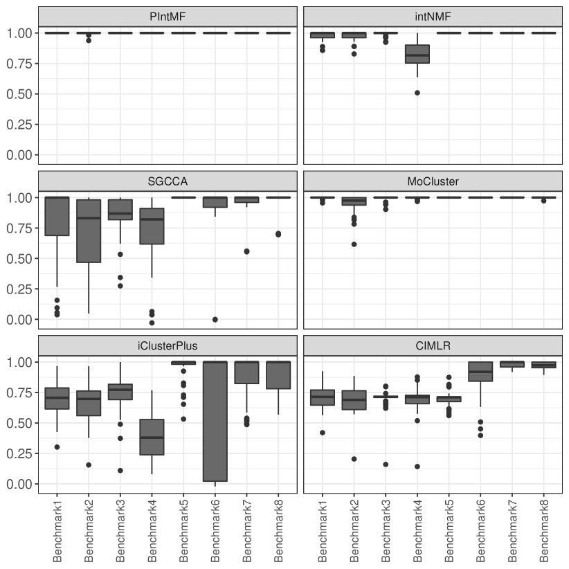
Four unbalanced groups (composed of 25, 20, 5, and 10 individuals) have been simulated (Benchmarks 1 to 5). Datasets with 2, 3, and 4 balanced groups have also been simulated (Benchmarks 6 to 8). Each benchmark is simulated 50 times.

PIntMF was compared to several integrative unsupervised methods (Pierre-Jean et al., 2019) that perform both clustering and variable selection namely: intNMF (Chalise et al., 2014), SGCCA (Tenenhaus et al., 2014), MoCluster (Meng et al., 2015), iClusterPlus (Mo et al., 2013), and CIMLR (Ramazzotti et al., 2018).

Clustering performance was evaluated using the Adjusted Rand Index on simulated data (see section 3.1).

On the eight simulated benchmarks with various levels of signal to noise ratio, PIntMF and MoCluster outperform the other methods with an ARI equal to 1 in most cases (Fig. 1).

Figure 1: Adjusted Rand Index of PIntMF, intNMF, SGCCA, MoCluster, iClusterPlus, and CIMLR methods on simulated datasets. B1 :Referrence, B2: More Gaussian noise, B3: More Gaussian noise and more Binary noise, B4: More Beta noise and more Binary noise, B5: More Relevant variables, B6: 2 balanced groups, B7: 3 balanced groups, B8: 4 balanced groups

The performance of variable selection is assessed using the area under ROC curves (AUROC) after computing False Positive Rates (FPR) and True Positive Rates (TPR) (see section 3.2). The computation of the AUROC shows that PIntMF performs as well as MoCluster on the three types of data (Table S1 in Supplementary Materials). Indeed, PIntMF reaches either the first or the second-best AUROC for these simulations. Besides, the lowest AUROC is equal to 0.88 which means that the method is both sensitive and specific.

4.2.2 Simulation based on real data (correlated blocks)

We evaluate the performance of PIntMF on a simulated framework based on cancer real data and developed by (Chung and Kang, 2019). Indeed, the previous framework does not simulate any correlation between omics blocks.

OmicsSIMLA is a simulation tool for generating multi-omics data with disease status. This tool simulates CpGs with methylation proportions, RNA-seq read counts and normalized protein expression levels. Here, we simulated 50 datasets containing 50 cases (i.e., short-term survival) and 50 controls (i.e. long-term survival), and three omics blocks (RNAseq, DNA methylation, and proteins). We try to recover the two groups but also the different features that drive overall survival by using DNA methylation, expression, and protein data. For two of the three blocks (expression and DNA methylation), the variables differentially expressed or methylated between the two groups are known.

The simulated data are described in Supplementary Materials (Section 5).

In these simulations, we also compare the performance of PIntMF to other methods in terms of clustering and variable selection. First, CIMLR does not give any results on these simulations (the algorithm does not converge). For all the other methods, the ARI is equal to 1 (maximum value) for all 50 datasets.

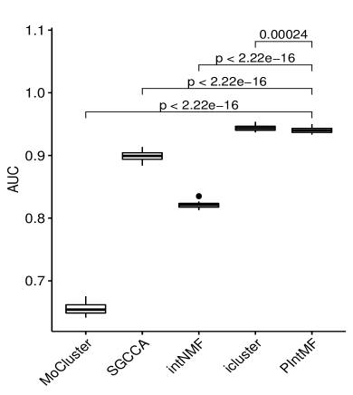
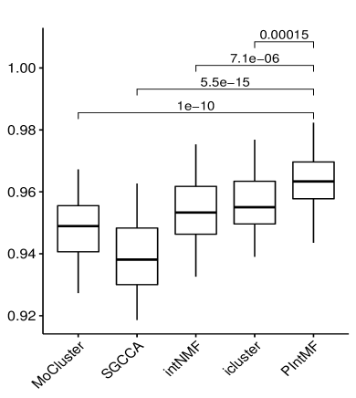
Then, we compare the variable selection performance of PIntMF, intNMF, iClusterPlus, MoCluster, and SGCCA by computing the AUROC on expression and DNA methylation blocks only (the protein block does not contain any variable simulated with differential abundance, more details are given in Supplementary Materials section 5).

DNA Methylation dataset: PintMF and iclusterPlus outperform the others with similar performances but the AUROC of iclusterPlus is significantly higher. Then, the AUROC of PintMF is significantly higher than for MoCluster, SGCCA and intNMF (Fig. 2).

Expression dataset: PIntMF is the best method with an AUROC significantly higher than the others. However, all methods achieve an AUROC higher than 0.92. (Fig. 2)

On these simulations, PIntMF gives similar results to iClusterPlus, but with automatic tuning of parameters. Besides, the algorithm of PIntMF is faster than iClusterPlus.

(a) Methylation

(b) Expression

Figure 2: AUROC of PIntMF, MoCluster, SGCCA, iClusterPlus and intNMF for OmicsSIMLA simulations on (a) DNA methylation and (b) Gene expression blocks

4.2.3 Stability selection

Jackknife was performed to evaluate the stability of variable selection. To perform this technique, we run the model PIntMF on the data without one sample at each step. Therefore, we obtain $n$ datasets containing $n-1$ individuals on which we apply the method.

The stability of the selected variables for Binary, Gaussian, methylation and expression datasets seems to be strong (Fig. S10 in Supplementary Materials). For proteins and for beta-like data, the bootstrap reveals that some selected variables are not stable. The Jackknife method could be used to remove false-positives variables.

4.2.4 Summary

To summarize this simulation part (see Table 1), our method PIntMF provides satisfying clustering and variable selection both on correlated blocks (Simulation Framework 2) and on non-correlated blocks (Simulation Framework 1). PIntMF is the only method that performs well on all simulated settings.

We conclude on these two frameworks of simulated data that PIntMF is a fast and flexible tool.

	Clustering	Variable selection	Automatic Tunning	Parameters left to tune
iClusterPlus	+	++	-	¿2
intNMF	+++	-	+++	1
SGCCA	++	++	-	¿5
MoCluster	+++	+++	+	¿2
CIMLR	+	++	+++	1
PIntMF	+++	+++	+++	1

Table 1: Summary of the performance of the PIntMF compared to other methods

4.3 Applications

In this section, we assess the performance of the PIntMF method on real data by considering two applications. The first one is a dataset from murine liver (Williams et al., 2016) under two different diets already used in two previous comparison articles (Pierre-Jean et al., 2019; Tini et al., 2017), and the objective is to recover the diets of the mice (fat diet or chow diet). The second one is a glioblastoma dataset from TCGA used in (Shen et al., 2012) and the goal is to find the tumor subtypes.

4.3.1 PIntMF highlights variables linked to phenotypes of samples

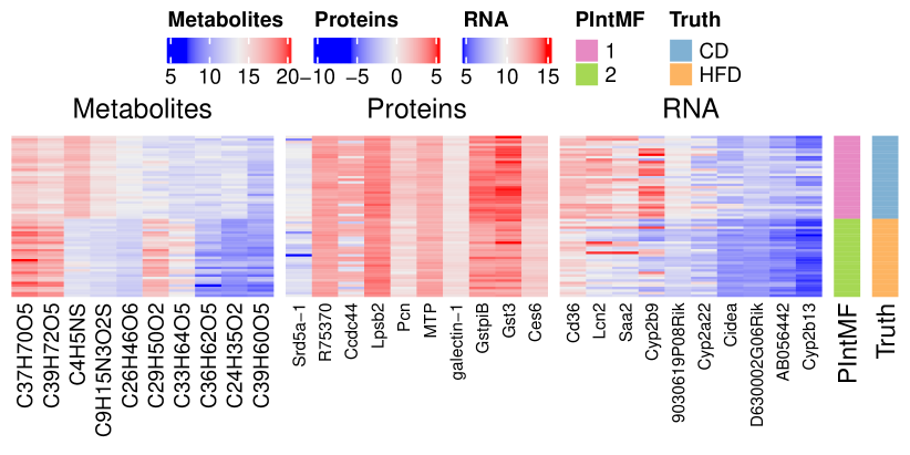
We analyzed the BXD cohort (composed of 64 samples) (Williams et al., 2016); the mice were shared into two different environmental conditions of diet: chow diet (CD) (6% kcal of fat) or high-fat diet (HFD) (60% kcal of fat). Measurements have been made in the livers of the entire population at the transcriptome, the proteome, and the metabolome levels.

Therefore, we applied PIntMF to this dataset as well as intNMF, MoCluster, SGCCA, iClusterPlus, and CIMLR (Supplementary Materials Table S2).

PIntMF produces a perfect classification of the individuals for this real dataset .

For this dataset, all criteria for the model selection were computed (Supplementary Material Fig. S6), and 2 groups were selected for further analysis.

PIntMF highlights interesting variables that seem to have different abundance between the two groups CD and HFD (Fig. 3): VITAMIN E (C${}_{2}9$H${}_{5}0$0₂), Cholesteryl (C${}_{3}6$H${}_{6}2$O₅), Mustard Oil (C₄H₅NS). Saa2 gene that codes for a protein involved in the HDL complex seems to be deferentially expressed between the two groups. Then, the Cidea gene that is involved in the metabolism of lipids and lipoproteins has a slightly different level of expression between the two groups. Finally, Cyp2b9 oxidies steroids, fatty acids, and xenobiotics are less expressed in the high-fat diet group. To conclude, PIntMF succeeds well to recover classification and relevant markers in all datasets.

Figure 3: BXD cohort results: Top 10 selected variables with PIntMF of each dataset (Metabolites, Proteins and RNA), the clustering given by PIntMF and the true clustering are on the right.

4.3.2 PIntMF reveals a new classification of non annotated samples on TCGA dataset.

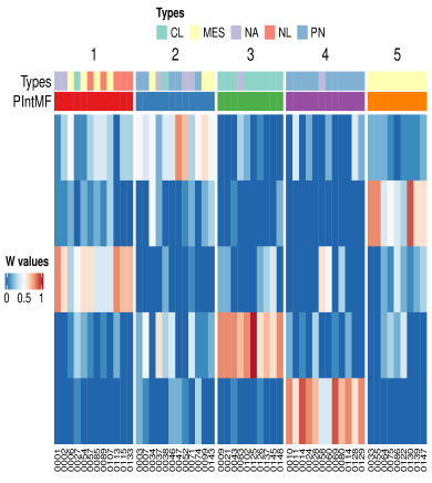
Secondly, we analyze a subset of the glioblastoma dataset from the cancer genome atlas (TCGA): the Glioblastoma study (2009) used in (Shen et al., 2012). The dataset contains three matrices: copy number variation (1599 regions), DNA methylation (1515 CpG), and mRNA expression (1740 genes) in 55 samples. GBM samples were classified into four subtypes (Classical: CL, Mesenchymal: MES, Neural: NL, and Proneural: PN). Besides, there are samples with no subtype (NA). Using the PIntMF method, we highlight samples with no classification close to labeled samples. Looking at the three criteria, the best number of latent variables seems to be 5 (Supplementary Materials Fig. S7). For example, the green cluster from PIntMF matches a part of the CL subtype, and one sample labeled as NA is in this green cluster. Then, the purple cluster from PIntMF matches the PN subtype, and one sample labeled as NA can be classified with the PN subtype (Figure 4a). Clusters 1 (red) and 2 (blue) are more heterogenous. However, the red one is composed of NL and NA labeled samples. The blue one is close to samples labeled as PN.

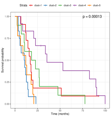
We performed a survival analysis to identify a relation between groups found by PIntMF and the survival rate (Figure 4b). The survival test gives a significant p-value at 5% (p-value =0.00013 with log-rank test). The prognosis for the purple (4) group is better than those of the red and green (1 and 3) groups and even better than the orange and blue (2 and 5) groups. Note that the PN subtype is split into two groups (purple and blue) that have two very different survival curves.

The previous study (Shen et al., 2012) performed with iCluster method (Shen et al., 2009) identified 3 subgroups with a less significant p-value (0.01) than PIntMF for the survival differences between subgroups. Their Cluster 1 matches the PN group, Cluster 2 matches the CL group, and Cluster 3 is mostly composed of the MES subtype. Authors do not give any information about the samples with no subtypes.

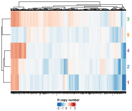
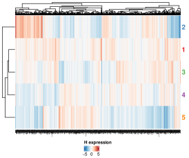
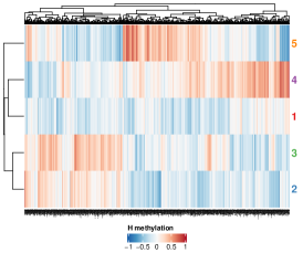
$\mathbf{H}$ matrices exhibit various types of genomic profiles according to the clusters (Figure 4). For instance, the orange cluster (5) shows few alterations at the copy number variation level (Fig. 4c) but a particular profile for DNA methylation and gene expression data (Fig. 4e). The blue cluster (2) has a distinct pattern of expression (Fig. 4d).

(a) Heatmap plot of $\mathbf{W}$: Homogeneity between subtypes and subgroups identified by PIntMF

(b) Kaplan-Meier plot: The subgroups identified by PIntMF show survival differences

(c) Copy number variation

(d) Gene Expression

(e) DNA Methylation

Figure 4: (a) Heatmap of $\mathbf{W}$. The clustering of PIntMF was compared to glioblastoma subtypes. (b) Survival curves with p-value of log-rank test. (c, d, e) $\mathbf{H}$ matrix for the three considered omics blocs on glioblastoma dataset

5 Discussion

We presented a new model to discover new subgroups of a cohort and potential new markers from several types of omic data. PIntMF is a matrix factorization model with positivity and sparsity constraints (Lasso) on inferred matrices. The method and all scripts of this article are available in an R package named PIntMF.

The main advantage of this method is the automatic tuning of the lasso penalties for both variable and sample matrices. To optimize the algorithm at the computational time level (Supplementary Materials Fig.S9), we tried several algorithms to infer matrices $\mathbf{H}^{k}$. glmnet is very fast compared to the others (ncvreg, quadrupen, and biglasso), therefore it was retained for all analysis. We also optimized the initialization of the algorithm that is obtained by using the SNF algorithm (Wang et al., 2014). This initialization provides, at the end of the algorithm, the best clustering and the best percentage of explained variation (Fig. S1). Besides, this initialization is performed at the integrative level rather than separately on each block of data.

PIntMF tunes automatically the penalties on matrices $\mathbf{H}^{k}$ and $\mathbf{W}$, without any intervention of the user, and we noticed that all the matrices are quite sparse on real datasets (Figure 4). The user needs to choose only one parameter that is the number of latent variables. The last parameter can be chosen by looking at the MSE, cophenetic coefficient, and the PVE (Supplementary Materials Fig. S2 to S6). All these criteria are implemented in the R package. For non-correlated data simulations, only the cophenetic coefficient and the PVE allow choosing properly the correct number of latent variables.

It is still difficult to evaluate the performance of an integrative method on simulations (Cantini et al., 2020). The relationships between blocks of omics are complex, often not well-known, and the modeling of these links is not easy. To our knowledge, there does not exist any reference dataset to assess performances. Therefore, we evaluated the algorithm on two different simulation frameworks (completely simulated and based on real-data) and two real datasets. Besides, we compared it with several other state-of-the-art integrative methods. We demonstrated, on the first simulated dataset (non-correlated blocks), that PIntMF outperforms the other methods on both clustering and variable selection. Indeed, on simulated data, the clustering from PIntMF makes few errors of classification. We also highlighted that PIntMF is more robust to heterogeneous data compared to the others: the method performs as well on gaussian distributions as on binary or beta distributions for the variable selection. On another simulated framework based on real data (correlated blocks), we observed good performances at clustering (perfect classification) and variable selection levels (AUROC upper than 90%). With applications on two real datasets (BXD and TCGA data section 4.3), we demonstrated that the method could deal with real datasets. Besides, the application on the two real datasets shows that we found original subgroups but also interesting variables linked to the clinical phenotypes (diet and overall survival).

A weakness of the model is that the convergence of the algorithm to an optimal solution is not mathematically justified. Besides, a significance test for the variable selection is not given due to the use of the LASSO regression (Jain and Xu, 2021). Jackknife could provide an idea of the confidence in the selected variables (Supplementary Materials Fig. S10). However, this type of approach is very time-consuming when datasets are large.

Another improvement of the method could be dealing with missing values. Missing values could be inside a block for a few variables. These missing values could be imputed by the average of other correlated variables or by the values of the nearest neighbor or more complex methods as proposed by (Voillet et al., 2016; González et al., 2009; Husson and Josse, 2013). Commonly, a whole block can also be missing for an individual. In this case, the matrix $\mathbf{W}$ could be computed only on the present blocks for this individual. Thanks to the $\mathbf{W}$ matrix, we could deduce a new profile for this patient from the $\mathbf{H}^{k}$ matrix inferred with the other individuals.

We could also extend PIntMF by including prior information such as the genome structure. For instance, we could force the algorithm to select the same genes in the DNA methylation block and the expression block. A group Lasso penalty (Simon et al., 2013) could be added to the proposed model to include such a prior.

To conclude, PIntMF is an easy and flexible method to integrate omics data. It exhibits good performance in terms of classification or variable selection in both cases (correlated blocks or non-correlated blocks). Among all tested methods, it is the one that works in most situations. PIntMF is fast and automatically tunes the penalty for each block to select an appropriate number of variables (sparse matrices). Besides, it provides a sparse matrix $\mathbf{W}$ to perform more easily the clustering of samples. We also provide three criteria namely MSE, PVE, and cophenetic coefficient to choose the best number of latent variables.

The integration of several types of omics with our method could help in discovering potential markers even with a small number of patients. Finally, it could also help to classify patients with unknown phenotypes.

6 Software

An R package named PIntMF can be used to reproduce all simulations and figures and is available online at ??.

References

- Bersanelli et al. (2016) Bersanelli, M., Mosca, E., Remondini, D., Giampieri, E., Sala, C., Castellani, G., and Milanesi, L. (2016). Methods for the integration of multi-omics data: mathematical aspects. BMC bioinformatics, 17(Suppl 2), 15.
- Bock et al. (2016) Bock, C., Farlik, M., and Sheffield, N. C. (2016). Multi-omics of single cells: strategies and applications. Trends in biotechnology, 34(8), 605–608.
- Brunet et al. (2004) Brunet, J.-P., Tamayo, P., Golub, T. R., and Mesirov, J. P. (2004). Metagenes and molecular pattern discovery using matrix factorization. Proceedings of the national academy of sciences, 101(12), 4164–4169.
- Burstein et al. (2015) Burstein, M. D., Tsimelzon, A., Poage, G. M., Covington, K. R., Contreras, A., Fuqua, S. A., Savage, M. I., Osborne, C. K., Hilsenbeck, S. G., Chang, J. C., et al. (2015). Comprehensive genomic analysis identifies novel subtypes and targets of triple-negative breast cancer. Clinical Cancer Research, 21(7), 1688–1698.
- Cantini et al. (2020) Cantini, L., Zakeri, P., Hernandez, C., Naldi, A., Thieffry, D., Remy, E., and Baudot, A. (2020). Benchmarking joint multi-omics dimensionality reduction approaches for cancer study. Nature Communications.
- Chalise and Fridley (2017) Chalise, P. and Fridley, B. L. (2017). Integrative clustering of multi-level omic data based on non-negative matrix factorization algorithm. PloS one, 12(5), e0176278.
- Chalise et al. (2014) Chalise, P., Koestler, D. C., Bimali, M., Yu, Q., and Fridley, B. L. (2014). Integrative clustering methods for high-dimensional molecular data. Translational cancer research, 3(3), 202.
- Chauvel et al. (2019) Chauvel, C., Novoloaca, A., Veyre, P., Reynier, F., and Becker, J. (2019). Evaluation of integrative clustering methods for the analysis of multi-omics data. Briefings in Bioinformatics.
- Chen and Zhang (2018) Chen, J. and Zhang, S. (2018). Discovery of two-level modular organization from matched genomic data via joint matrix tri-factorization. Nucleic acids research, 46(12), 5967–5976.
- Chung and Kang (2019) Chung, R.-H. and Kang, C.-Y. (2019). A multi-omics data simulator for complex disease studies and its application to evaluate multi-omics data analysis methods for disease classification. GigaScience, 8(5), giz045.
- Gaujoux and Seoighe (2010) Gaujoux, R. and Seoighe, C. (2010). A flexible r package for nonnegative matrix factorization. BMC bioinformatics, 11(1), 367.
- González et al. (2009) González, I., Déjean, S., Martin, P. G., Gonçalves, O., Besse, P., and Baccini, A. (2009). Highlighting relationships between heterogeneous biological data through graphical displays based on regularized canonical correlation analysis. Journal of Biological Systems, 17(02), 173–199.
- Huang et al. (2017) Huang, S., Chaudhary, K., and Garmire, L. X. (2017). More is better: recent progress in multi-omics data integration methods. Frontiers in genetics, 8, 84.
- Husson and Josse (2013) Husson, F. and Josse, J. (2013). Handling missing values in multiple factor analysis. Food quality and preference, 30(2), 77–85.
- Jain and Xu (2021) Jain, R. and Xu, W. (2021). Hdsi: High dimensional selection with interactions algorithm on feature selection and testing. PLOS ONE, 16(2), 1–17.
- Jerome et al. (2010) Jerome, F., Trevor, H., and Robert, T. (2010). Regularization paths for generalized linear models via coordinate descent. Journal of Statistical Software, 33(1), 1–22.
- Lee and Seung (1999) Lee, D. D. and Seung, H. S. (1999). Learning the parts of objects by non-negative matrix factorization. Nature, 401(6755), 788.
- Meng et al. (2015) Meng, C., Helm, D., Frejno, M., and Kuster, B. (2015). mocluster: Identifying joint patterns across multiple omics data sets. Journal of proteome research, 15(3), 755–765.
- Mo and Shen (2018) Mo, Q. and Shen, R. (2018). iClusterPlus: Integrative clustering of multi-type genomic data. R package version 1.18.0.
- Mo et al. (2013) Mo, Q., Wang, S., Seshan, V. E., Olshen, A. B., Schultz, N., Sander, C., Powers, R. S., Ladanyi, M., and Shen, R. (2013). Pattern discovery and cancer gene identification in integrated cancer genomic data. Proceedings of the National Academy of Sciences, 110(11), 4245–4250.
- Network et al. (2012) Network, C. G. A. et al. (2012). Comprehensive molecular portraits of human breast tumours. Nature, 490(7418), 61.
- Nowak et al. (2011) Nowak, G., Hastie, T., Pollack, J. R., and Tibshirani, R. (2011). A fused lasso latent feature model for analyzing multi-sample acgh data. Biostatistics, 12(4), 776–791.
- Pierre-Jean et al. (2019) Pierre-Jean, M., Deleuze, J.-F., Le Floch, E., and Mauger, F. (2019). Clustering and variable selection evaluation of 13 unsupervised methods for multi-omics data integration. Briefings in bioinformatics.
- Ramazzotti et al. (2018) Ramazzotti, D., Lal, A., Wang, B., Batzoglou, S., and Sidow, A. (2018). Multi-omic tumor data reveal diversity of molecular mechanisms that correlate with survival. Nature communications, 9(1), 4453.
- Rand (1971) Rand, W. M. (1971). Objective criteria for the evaluation of clustering methods. Journal of the American Statistical association, 66(336), 846–850.
- Reilly et al. (2019) Reilly, B., Tanaka, T. N., Diep, D., Yeerna, H., Tamayo, P., Zhang, K., and Bejar, R. (2019). Dna methylation identifies genetically and prognostically distinct subtypes of myelodysplastic syndromes. Blood advances, 3(19), 2845–2858.
- Ritchie et al. (2015) Ritchie, M. D., Holzinger, E. R., Li, R., Pendergrass, S. A., and Kim, D. (2015). Methods of integrating data to uncover genotype–phenotype interactions. Nature Reviews Genetics, 16(2), 85.
- Rodosthenous et al. (2020) Rodosthenous, T., Shahrezaei, V., and Evangelou, M. (2020). Integrating multi-omics data through sparse canonical correlation analysis for the prediction of complex traits: A comparison study. Bioinformatics.
- Rowlands et al. (2014) Rowlands, D. S., Page, R. A., Sukala, W. R., Giri, M., Ghimbovschi, S. D., Hayat, I., Cheema, B. S., Lys, I., Leikis, M., Sheard, P. W., et al. (2014). Multi-omic integrated networks connect DNA methylation and miRNA with skeletal muscle plasticity to chronic exercise in type 2 diabetic obesity. Physiological genomics, 46(20), 747–765.
- Sastry et al. (2020) Sastry, A. V., Hu, A., Heckmann, D., Poudel, S., Kavvas, E., and Palsson, B. O. (2020). Matrix factorization recovers consistent regulatory signals from disparate datasets. BioRxiv.
- Shen et al. (2009) Shen, R., Olshen, A. B., and Ladanyi, M. (2009). Integrative clustering of multiple genomic data types using a joint latent variable model with application to breast and lung cancer subtype analysis. Bioinformatics, 25(22), 2906–2912.
- Shen et al. (2012) Shen, R., Mo, Q., Schultz, N., Seshan, V. E., Olshen, A. B., Huse, J., Ladanyi, M., and Sander, C. (2012). Integrative subtype discovery in glioblastoma using icluster. PloS one, 7(4), e35236.
- Simon et al. (2013) Simon, N., Friedman, J., Hastie, T., and Tibshirani, R. (2013). A sparse-group lasso. Journal of computational and graphical statistics, 22(2), 231–245.
- Sneath et al. (1973) Sneath, P. H., Sokal, R. R., et al. (1973). Numerical taxonomy. The principles and practice of numerical classification.
- Sokal and Rohlf (1962) Sokal, R. R. and Rohlf, F. J. (1962). The comparison of dendrograms by objective methods. Taxon, pages 33–40.
- Tenenhaus and Tenenhaus (2011) Tenenhaus, A. and Tenenhaus, M. (2011). Regularized generalized canonical correlation analysis. Psychometrika, 76(2), 257–284.
- Tenenhaus et al. (2014) Tenenhaus, A., Philippe, C., Guillemot, V., Le Cao, K.-A., Grill, J., and Frouin, V. (2014). Variable selection for generalized canonical correlation analysis. Biostatistics, 15(3), 569–583.
- Tibshirani (1996) Tibshirani, R. (1996). Regression shrinkage and selection via the lasso. Journal of the Royal Statistical Society. Series B (Methodological), pages 267–288.
- Tini et al. (2017) Tini, G., Marchetti, L., Priami, C., and Scott-Boyer, M.-P. (2017). Multi-omics integration - a comparison of unsupervised clustering methodologies. Briefings in bioinformatics.
- Vasaikar et al. (2017) Vasaikar, S. V., Straub, P., Wang, J., and Zhang, B. (2017). Linkedomics: analyzing multi-omics data within and across 32 cancer types. Nucleic acids research, 46(D1), D956–D963.
- Voillet et al. (2016) Voillet, V., Besse, P., Liaubet, L., San Cristobal, M., and González, I. (2016). Handling missing rows in multi-omics data integration: multiple imputation in multiple factor analysis framework. BMC bioinformatics, 17(1), 1–16.
- Wang et al. (2014) Wang, B., Mezlini, A. M., Demir, F., Fiume, M., Tu, Z., Brudno, M., Haibe-Kains, B., and Goldenberg, A. (2014). Similarity network fusion for aggregating data types on a genomic scale. Nature methods, 11(3), 333.
- Ward Jr (1963) Ward Jr, J. H. (1963). Hierarchical grouping to optimize an objective function. Journal of the American statistical association, 58(301), 236–244.
- Williams et al. (2016) Williams, E. G., Wu, Y., Jha, P., Dubuis, S., Blattmann, P., Argmann, C. A., Houten, S. M., Amariuta, T., Wolski, W., Zamboni, N., et al. (2016). Systems proteomics of liver mitochondria function. Science, 352(6291), aad0189.
- Yang (2020) Yang, X. (2020). Multitissue multiomics systems biology to dissect complex diseases. Trends in Molecular Medicine.
- Yugi et al. (2016) Yugi, K., Kubota, H., Hatano, A., and Kuroda, S. (2016). Trans-omics: how to reconstruct biochemical networks across multiple omic layers. Trends in biotechnology, 34(4), 276–290.