Optimising the mitigation of epidemic spreading through targeted adoption of contact tracing apps

Abstract

The ongoing COVID-19 pandemic is the first epidemic in human history in which digital contact-tracing has been deployed at a global scale. Tracking and quarantining all the contacts of individuals who test positive to a virus can help slowing-down an epidemic, but the impact of contact-tracing is severely limited by the generally low adoption of contact-tracing apps in the population. We derive here an analytical expression for the effectiveness of contact-tracing app installation strategies in a SIR model on a given contact graph. We propose a decentralised heuristic to improve the effectiveness of contact tracing under fixed adoption rates, which targets a set of individuals to install contact-tracing apps, and can be easily implemented. Simulations on a large number of real-world contact networks confirm that this heuristic represents a feasible alternative to the current state of the art.

Since the first human infection towards the end of 2019, the spread of the SARS-COV-2 virus has caused an unprecedented shock around the world, with serious repercussions in all aspects of our social and economic activities mckibbin2020economic ; mckibbin2020global ; holman2020unfolding , and a number of casualties that has already passed the two millions figure and is unfortunately due to rise further in the near future mega2020covid . The initial efforts to curb the spread of the disease focused on non-pharmaceutical interventions including travel bans, lockdowns, and curfewsPerra2021 . These measures are able to drastically reduce the opportunities of contacts between infected and susceptible people and thus the spread of a virus balcan2009 ; riley2007 ; ferguson2005 ; colizza2007 ; PastorSatorras2015 , but also have non-negligible effects on the economy and social life flaxman2020estimating ; cowling2020impact ; peak2017comparing . After the first wave of infections in February-May 2020 and thanks to a better understanding of the specific transmission dynamics of SARS-COV-2 arenas2020 ; chang2020mobility ; di2020impact ; wiersinga2020pathophysiology ; haug2020 ; aguilar2020impact , many countries have implemented some sort of “test-trace-treat” system based on digital contact tracing rodriguez2021population ; bradshaw2021bidirectional . Some of these systems consist on deploying contact tracing (CT) apps on mobile phones which allow to identify and isolate individuals who have been in contact with infected ones, thus disrupting secondary infections paths as early as possible. With contact tracing in place, many countries have been able to partially re-open several sectors of their economy and to diminish the damage of prolonged disruptions aleta2020 ; panovska2020determining ; cohen2020countries ; abueg2020modeling ; jiang2020survey ; kerr2020controlling ; kucharski2020effectiveness ; smith2020adherence

An effective digital contact tracing strategy should aim at maximising the probability of detecting contacts between infected and susceptible individuals, and it would completely eradicate contagion in the ideal case where CT apps are installed by the totality of a population eames2003contact ; klinkenberg2006effectiveness ; kretzschmar2020impact ; ferretti2020quantifying ; keeling2020efficacy ; park2020contact ; barrat2020CT ; gardenes2020spreadingCT ; kryven2020CT ; bianconi2020messageapps . However, throughout the SARS-COV-2 pandemic the percentage of the population with CT apps installed has remained quite low, between 5% and 20% in most countries StatistaCTPerc , resulting in a dramatically decreased efficiency of contact-tracing.

Here we focus on the problem of determining the set of nodes which should install CT apps in order to optimise the effect of contact tracing, i.e., to maximally slow-down spreading and reduce the incidence of a disease, under the assumption that the rate of CT app adoption is fixed. We provide an analytic derivation to quantify the decrease of the basic reproduction number caused by a generic CT installation strategy, and we show that uniform random installation – which is the strategy implicitly adopted by governments when people are simply asked to install a CT app – has the worst performance of all. We find that relatively simple targeting strategies based on the structure of the contact network are significantly more efficient in reducing the number of secondary infections at low adoption rates, in both synthetic and real-world systems.

Figure 1: Effect of contact-tracing apps on secondary infections on a contact network. Contact tracing apps can only detect potential contagious contacts if both the infected and the susceptible individual have a CT app installed. In this case, A can in principle infect any of his direct neighbours, including B who has a CT app installed as well, and the CT app cannot do anything to avoid this. However, if the CT system detects a contact between A and B and then A tests positive, then B can be contacted and put into quarantine, thus disrupting all the potential infection paths to the direct contacts of B (solid green lines). If C has a contact with A, instead, C has no way of knowing whether the contact resulted in an infection or not, he will not be notified when A tests positive, and he will not go into quarantine. In this case, all the neighbours of C are at risk of catching the disease (solid red lines). Similarly, the fact that B has a CT app installed cannot safeguard her from being infected by D (who does not have a CT app installed) and passing the infection to her neighbours while she has no symptoms.

Results

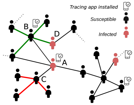
In Fig. 1 we report a sketch of a fictious contact network, where some individuals are infected (pink), some other are susceptible (black), and some have a CT app installed (indicated by the mobile icon). A perfect lockdown would remove almost all the links in that graph (with the only exception of those among people belonging to the same household), so that infected individuals will eventually be unable to find any susceptible person to pass the disease on. When only contact tracing is in place, instead, some infections are still unavoidable, either due to a limited app adoption rate or to a delay in the notification of test results and in isolation of subjects exposed to infected ones. As made evident by Fig. 1, maximising the impact of contact tracing corresponds to maximising the probability that the potential transmission of the disease between two individuals is detected, since only contacts among people with CT apps installed can be detected and traced back. This intuitively corresponds to maximising the number of edges among the individuals with CT app installed, i.e., the density of the subgraph induced by the nodes with CT apps, under the constraint that only a fraction $r$ of the population will have the CT app installed.

Figure 2: Effect of different CT strategies on the induced subgraph as a function of app adoption rate $r$. (a) The ratio ${R^{\prime}_{0}}/{R_{0}}$ as a function of the CT adoption rate $r$ for the Random (RND), degree-based (DEG), distributed targeting (DTI), and Simulated Annealing (SA) strategies, calculated using Eq. (1). (b) Average degree of $G^{\prime}$ as a function of the adoption rate $r$ for each of the strategies. The theoretical predictions for the RND and DEG strategies (solid lines) were obtained using Eq. (7) and Eq. (17), respectively. (c) Second moment of the degree distribution of $G^{\prime}$ as a function of the adoption rate $r$ for each of the strategies. The plots correspond to an ensemble of configuration model graphs with degree distribution $P(k)\sim k^{-3}$ and $N=10^{4}$ nodes. Results averaged over 100 realisations.

Reduction of $R_{0}$ in a SIR+CT dynamics. We consider here a SIR+CT model, which is a classical Susceptible-Infected-Recovered (SIR) model on a static contact graph PastorSatorras2015 , with the addition of ideal contact tracing. This means that any susceptible node with installed CT app is quarantined (recovered) as soon as one of their contacts with CT app installed gets infected. The parameters of the model are the probability $\beta$ that an infected individual passes the disease to each of its susceptible neighbours, and the probability $\mu$ that an infected individual is removed (due to either recovery or death). We call the contact graph $G(V,E)$, with $N=|V|$ nodes and $K=|E|$ edges, and we denote by $G^{\prime}(V^{\prime},E^{\prime})$ the subgraph of $G$ induced by CT app installations, i.e., such that $V^{\prime}$ is the set of nodes in $G$ with CT apps and $E^{\prime}$ is the set of edges among nodes in $V^{\prime}$. We quantify the effect of the installation of CT apps in a certain subset $V^{\prime}$ of nodes by computing the reduction of the basic reproduction number $R_{0}$, that is the expected number of secondary infections caused by a single contagion event. Let us assume that the generic node $\ell$ is infected and has passed the disease to its neighbour $i$. The expected number $R_{i}$ of secondary infections caused by $i$ while it remains infected depends on whether $i$ is in $V^{\prime}$, and on how many of its $k_{i}$ neighbours are in $V^{\prime}$ as well. In particular, if $i\notin V^{\prime}$, $R_{i}=\frac{\beta}{\mu}(k_{i}-1)$ as in the classical SIR (we have to remove $\ell$ from the count, hence the $k_{i}-1$) PastorSatorras2015 . If $i\in V^{\prime}$, instead, there are two possible cases: a) if $\ell\notin V^{\prime}$, the contact between $\ell$ and $i$ remains undetected, and $i$ can potentially infect $R_{i}=\frac{\beta}{\mu}(k_{i}-1)$ more nodes, as in the classical SIR. b) If instead $\ell\in V^{\prime}$ as well, then the contact with $i$ gets detected by the CT system and $i$ goes into self-isolation immediately, thus avoiding any secondary infection. If we denote by $k^{\prime}_{i}$ the degree of node $i$ in $G^{\prime}$, the expected number of infections potentially caused by the infection of $i$ is equal to

$$R_{i}=\frac{\beta}{\mu}(k_{i}-1)\frac{k_{i}-k_{i}^{\prime}}{k_{i}}$$

and the average number of secondary infections potentially caused by each node infected by $\ell$ is given by:

$$R_{\ell}=\frac{\beta}{\mu}\frac{1}{k_{\ell}}\sum_{i}a_{\ell i}(k_{i}-1)\frac{k_{i}-k_{i}^{\prime}}{k_{i}}$$

where $a_{\ell i}$ are the entries of the adjacency matrix of the contact graph $G$. By averaging $R_{\ell}$ over all the nodes of $G$ we obtain the value of the basic reproduction number in presence of contact tracing (see Methods for details):

$$\begin{array}[]{rl}R^{\prime}_{0}&=R_{0}-\frac{1}{N}\frac{\beta}{\mu}\sum_{\ell}\frac{1}{k_{\ell}}\sum_{i}a_{\ell i}\frac{k^{\prime}_{i}}{k_{i}}(k_{i}-1)\end{array}$$ (1)

where $R_{0}$ is the basic reproduction number of the classical SIR dynamics on $G$ PastorSatorras2015 . As made clear by Eq. (1), we can minimise the value of $R_{0}^{\prime}$ by using a generic optimisation algorithm to compute:

$$\max_{G^{\prime}}\quad\mathcal{F}(G^{\prime})=\sum_{\ell}\frac{1}{k_{\ell}}\sum_{i}a_{\ell i}\frac{k^{\prime}_{i}}{k_{i}}(k_{i}-1)$$ (2)

over the ensemble of possible choices of $G^{\prime}$. Notice that if the entire population installs CT apps (i.e., if $k^{\prime}_{i}=k_{i}\>\forall i\in V$) we trivially get $R^{\prime}_{0}=0$ (see Methods and Supplementary Note 1 for details).

CT targeting strategies. If we assume that we can install the contact tracing app only to a fraction $r\in[0,1]$ of “willing” individuals, Eq. (2) states that a good CT installation strategy should include in $G^{\prime}$ nodes having a high degree in $G$ (so that the ratio $\frac{(k_{i}-1)}{k_{i}}$ is as large as possible), and, at the same time, a high number of connections to other nodes in $G^{\prime}$ (i.e., so that $k^{\prime}_{i}$ is as large as possible). The most basic strategy to select a fraction $r$ of the $N$ individuals to install CT apps consists in asking the population to install a CT app in their mobile phones, under the assumption that each individual will comply with probability equal to $r$, irrespective of any of their specific social or behavioural characteristics. In this case, the total number of installations will be distributed according to a Binomial, with mean equal to $rN$. In the following, we call this strategy “uniform random installation” (RND).

A second strategy consists in explicitly targeting all the potential super-spreaders gomez2020mapping ; miller2020transmission . In practice, we ask the $rN$ individuals with the largest number of contacts (links) in $G$ to install the app, assuming that they will all comply with probability $1$. This strategy is indeed utopistic since it requires full knowledge of the contact network and full compliance by the selected nodes. In the following, we call this strategy “degree-based installation” (DEG).

Here we propose and study a constructive strategy to maximise Eq. (2) that does not require detailed global information on $G$, and is thus amenable to a distributed implementation. We start from a CT set that contains only the node with the largest degree in $G$. Then, at each subsequent step $t$ we add to the CT set one of the neighbours $i$ of any of the nodes in $V^{\prime}$, with probability proportional to the total number of neighbours of that node that are already in $V^{\prime}$ (see Methods for details). This creates a “social pressure” on individuals with no CT app installed which is proportional to the number of their contacts already in $V^{\prime}$. We call this strategy “distributed targeting installation” (DTI).

Figure 3: Impact of CT strategy and adoption rate on the epidemic peak of SIR+CT in real-world networks. The evolution of the disease in a SIR+CT model (here for $\beta=0.1$, $\mu=0.05$) depends heavily on the adoption rate $r$ and on the strategy used to select which individuals will have a CT app installed. We show here the results on two real-world social networks, namely, the high-resolution face-to-face contact data respectively recorded in a high school (a-d) and a workplace (e-h). We have applied a threshold to both contact networks: keeping only contacts larger than 240 seconds for the High School and 10% of the links with the largest weight for the Workplace (See Methods for details). At adoption rates $r\gtrsim 0.4$, the RND strategy (a, e) displays a higher percentage of infected compared to DTI (b, f), DEG (c, g) and SA (d, h). These differences are likely linked to the structure of the subgraph induced by each CT strategy. Typical examples of those graphs for each strategy and $r=0.3$ are shown in the insets, where the size of each node is proportional to its degree and nodes with CT app installed are indicated in blue.

In Fig. 2(a) we plot the ratio $\frac{R^{\prime}_{0}}{R_{0}}$ as a function of the CT adoption rate $r$ for the RND, DEG, and DTI strategies, on an ensemble of configuration model graphs with power-law degree distributions. As a reference, we also report the results obtained by optimising Eq. (2) by means of Simulated Annealing (SA). It is worth noting that RND is the worst-performing strategy overall, characterised by a much slower decrease of $R^{\prime}_{0}$ with $r$. Conversely, degree-based installation is close to the theoretical limit established by SA, and produces a noticeable decrease of $R_{0}$ already for quite small values of $r$. Remarkably, the performance of DTI is quite close to that of DEG, although DTI is not using any global information about the structure of $G$. In Fig. 2(b-c) we show how the first and second moment of the degree distribution $\widetilde{P}(k^{\prime})$ of the subgraph $G^{\prime}$ vary with $r$ for each of the four strategies. More details on the derivation of the full degree distribution of $G^{\prime}$ in RND and DEG are reported in Methods, while Supplementary Fig. 1 shows the perfect agreement between the empirical and analytical degree distributions for these two strategies.

It is worth noting that under the DEG strategy $\langle k^{\prime}\rangle$ increases very sharply with $r$ and is already quite similar to the value of $\langle k\rangle$ in $G$ for very small values of $r$. On the other hand, in RND $\langle k^{\prime}\rangle$ increases only linearly with $r$ (see Methods for details), while the performance of DTI is in between those two. However, these plots make it clear that the sheer density of $G^{\prime}$ is not the only important ingredient for CT app installation. Indeed, SA can attain consistently lower values of $\frac{R^{\prime}_{0}}{R_{0}}$ than DEG, although the values of $\langle k^{\prime}\rangle$ produced by SA are almost identical to that provided by DEG (see Fig. 2b).

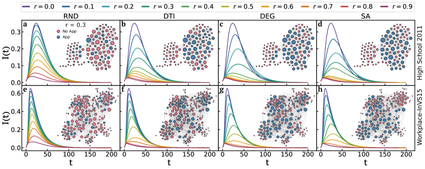
SIR+CT in real-world graphs. In Fig. 3 we show the ratio of infected nodes $I(t)$ for the four strategies with different values of $r$ on two real-world contact networks, respectively the network of friendship in a high school (top panels) and at a workplace (bottom panels)Sociopatterns . In the inset of each panel we report a typical composition of $V^{\prime}$ for each strategy. It is evident that, even at low adoption rates, the DEG and DTI strategy can heavily mitigate the incidence of the disease better than RND. This is most probably because DEG and DTI are targeting different sets of nodes than RND, and in general end up selecting nodes with high degree which result in a higher edge density in $G^{\prime}$.

Figure 4: Comparison of epidemic indicators under different CT strategies. Relative decrease with respect to random installations of the total number of recovered $\Delta R^{s}_{\infty}$, height of the infection peak $\Delta I^{s}(t_{\rm peak})$ and position of the peak $\Delta t^{s}_{\rm peak}$ (see Eq. (3)) for DTI, DEG, and SA targeted installation, in the same contact networks shown in Fig. 3. The inset of each panel reports the plot of the raw variable, respectively $R_{\infty}$ (panel a and d), $I(t_{\rm peak})$ (panel b and e) and $t_{\rm peak}$ (panel c and f).

The dynamics of SIR+CT in the two systems exhibits some noticeable qualitative differences when distinct strategies are adopted, with respect to the height of the infection peak (the maximum incidence of the disease), the actual position of the peak (the time at which it occurs), and the overall duration of the epidemic. Interestingly, the position of the peak shifts to the right (delays) at small values of $r$ for the DEG, DTI and SA strategies. Conversely, the peak starts to recede (it is anticipated) with respect to the baseline when $r$ becomes larger than a certain threshold, which depends on the particular structure of the contact network. While low values of $r$ lead to a delay in the dynamics – the peak shifts to the right – large enough values of $r$ effectively break the network into a number of disconnected components, resulting in a considerable disruption of the spreading – shift to the left.

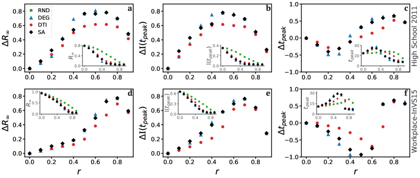
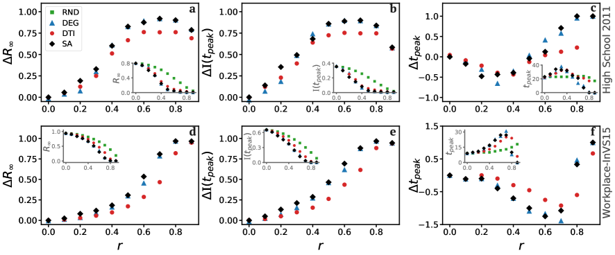
To better understand these qualitative differences, we look at three key properties of the epidemic curve, namely the total number of individuals recovered $R_{\infty}$, the maximum number of individuals infected across the duration of the epidemic $I(t_{\rm peak})$ and the time to reach the infection peak $t_{\rm peak}$. In particular, we compute the relative performance of each strategy $s$ (being it either DEG, DTI, and SA) with respect to RND using the quantities:

$$\begin{array}[]{rl}\Delta R^{s}_{\infty}&=1-\frac{R^{s}_{\infty}}{R^{\rm RND}_{\infty}}\\ \Delta I^{s}(t_{\rm peak})&=1-\frac{I^{s}_{t_{\rm peak}}}{I^{\rm RND}(t_{\rm peak)}}\\ \Delta t^{s}_{\rm peak}&=1-\frac{t^{s}_{\rm peak}}{t^{\rm RND}_{\rm peak}}\end{array}$$ (3)

The results are shown in Fig. 4. We found that in the high school network an adoption rate of $r=0.2$ can decrease the number of infected individuals at the peak by as much as 40% (Fig. 4b) for all the three strategies. At the same adoption rate, the total number of infected individuals decreases by 20% (Fig. 4a) and the peak is delayed by approximately 40% (Fig. 4c). For $r=0.5$ we witness a substantially stronger mitigation, where the peak is reduced by up to 70% and the total number of infected is reduced by up to 80%. The effectiveness of targeting strategies is somehow less pronounced in the workplace graph at similar adoption rates (bottom panels). Interestingly, in both networks the DTI strategy performs similarly to DEG and SA, as can be observed in the insets in Fig. 4, which show the raw values of $R_{\infty}$, $I(t_{\rm peak})$ and $t_{\rm peak}$.

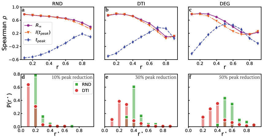
We simulated SIR+CT in 84 unique real-world contact network data sets, filtered by applying two different thresholds, for a total of 168 undirected graphs Starnini2013 ; vanhems2013 ; Barrat2014 ; Sociopatterns ; Genois2015 ; Genois2018 ; gadar2020multilayer ; sapiezynski2019interaction (See Methods for details). In Fig. 5(a-c), we report for the RND, DEG and DTI strategies, and several adoption rates $r$, the spearman correlation between the analytical $R^{\prime}_{0}$ and the epidemiological indicators $R_{\infty}$, $I(t_{\rm peak})$ and $t_{\rm peak}$. The correlation with both $R_{\infty}$ and $I(t_{\rm peak})$ is high for the three strategies confirming the analytical predictions of Eq. (1) despite the small size of the graphs and the presence of degree-degree correlations. Still, as $r$ increases we observe a decrease in the correlations, likely due to finite size effects. The correlation between $R^{\prime}_{0}$ and $t_{\rm peak}$ displays a much richer behaviour: we start with a significant but negative correlation for small $r$, which changes sign until it reaches a maximum. We conjecture that the change of sign is related to the movement of the peak: while in the small-$r$ regime lower values of $R^{\prime}_{0}$ contribute to a delay of the peak, for larger values of $r$ we observe a stronger anticipation of the peak. The value $r_{\rm peak}$ at which the correlation peaks depends on the strategy in use, the more efficient it is, the lower is the value of $r_{\rm peak}$. The concrete value of $r_{\rm peak}$ seems thus related to a certain structural cutoff of the graphs.

In a realistic scenario, in which the adoption rate is not fixed but needs to be promoted, we might be more interested in the minimum adoption rate $r^{*}$ needed on each network to obtain a given reduction of the infection peak with respect to the absence of contact tracing. In Fig. 5(d-f) we report the histograms of the value of $r^{*}$ in DTI and RND across the 168 networks when we set a reduction in the peak $I(t_{\rm peak})$ of 10%, 30% and 50%, respectively. We found that DTI can achieve a reduction of 30% of the peak in 85% of the networks with an adoption rate smaller than $0.3$ (panel e), while the RND strategy would need an adoption rate of $0.5$ to achieve an equivalent reduction.

Figure 5: Correlations with network structural measures and performance of CT strategies to mitigate an epidemic. For the 168 real-world contact networks analysed, panels (a-c) report as a function of $r$ the Spearman rank correlation between the analytical value of $R^{\prime}_{0}$ (Eq. (1)) and the epidemiological indicators $R^{s}_{\infty}$ (purple), $I^{s}(t_{\rm peak})$ (orange) and $t^{s}_{\rm peak}$ (blue) for the RND (a), DEG (b) and DTI (c) strategies. Panels (d-f) show the distribution of minimum adoption ratios $r^{*}$ needed to produce a $10\%$ (d), $30\%$ (e) and $50\%$ (f) for the DTI (red) and RND (green) strategies. Overall, DTI largely outperforms RND, which is the strategy currently adopted by many governments.

While the strategies analysed here require some level of global information and full compliance by individuals to install the app, we have obtained qualitatively similar results with other decentralised strategies based on local information, and with a tunable level of compliance (see Supplementary Note 2 and Supplementary Figs. 2-7 for details). Moreover, qualitatively similar results are also obtained when considering a SIR+CT with maximum delay, i.e., where an individual with the CT app installed goes into quarantine only when it becomes infected (see Supplementary Note 3 and Supplementary Figs. 7-9).

Conclusion. We have shown here that the random CT app installation – considered in recent studies on the topic barrat2020CT ; gardenes2020spreadingCT ; kryven2020CT and adopted by many governments – is the less effective strategy to mitigate the effects of a pandemic through contact tracing. The theoretical argument presented here, which links the reduction of $R_{0}$ to the structure of the subgraph $G^{\prime}$ induced by CT, holds for any graph under any CT strategy. In particular, Eq. 1 provides a concrete recipe to maximise the effectiveness of a CT app deployment as we have shown in real-world systems.

The reduction of a disease incidence attainable by the DTI strategy is comparable with degree-based targeting, which performs similarly to the optimal targeting obtained through simulated annealing. A notable advantage of using DTI over DEG is that it does not require any global information about the graph $G$ and it can be implemented on a distributed manner. For instance, one could ask every new individual who installs the CT app to broadcast a message to all his contacts, asking them to install it as well. By doing so, each contact with no app installed will be subject to a level of “social pressure” linearly proportional to the number of contacts who already have the CT app installed (in agreement with the heuristic algorithm of which DTI is based), consequently increasing the likelihood that he will also install it.

Although several effective vaccines have been made available recently jeyanathan2020immunological , mass vaccination campaigns are at their initial stage in many countries and might last for several months before a sufficient percentage of the population is vaccinated. Moreover, SARS-COV-2 variants may develop vaccine resistance and prolong the duration of the epidemic, creating an unsustainable loop of vaccine updates and vaccination campaigns. Hence, reducing the spreading of the virus by detecting potential infected individuals and limiting their contacts – through digital contact tracing – is still essential Gozzi2021importance . The results shown here suggest that governments could significantly improve the effectiveness of contact tracing programs by implementing targeting CT app installations, not only for the ongoing COVID-19 but any major epidemic event in the future.

Methods

Distributed Targeting Installation strategy

The proposed heuristic constructive algorithm to optimise Eq. (1), denominated DTI, starts with a set $V^{\prime}(t=0)$ containing the node of largest degree in $G$. At each step $t$, we consider the set $S(t)$ of nodes which have at least one neighbour in $V^{\prime}(t)$, then, a node $i$ is selected at $t+1$ from $S(t)$ and added to $V^{\prime}(t)$ with probability:

$$P(i;t)=\frac{\sum{j\in V^{\prime}(t)}a_{ij}}{\sum_{i\in S(t)}\sum_{j\in V^{\prime}(t)}a_{ij}}$$ (4)

i.e., node $i$ is selected linearly proportional to the number of neighbours it has in $V^{\prime}(t)$.

Properties of the subgraph induced by app installation

We provide here a sketch of the derivation of the first two moments of the degree distribution of the subgraph $G^{\prime}$ obtained from a graph $G$ by considering only the nodes which have the contact-tracing app installed and the edges among them. The full derivations are provided in Supplementary Note 1. In the case of random installation strategy, the probability that a node installs the contact tracing app is uniform across all nodes. As a consequence, the probability that a node with degree $k$ in $G$ has degree $k^{\prime}$ in $G^{\prime}$ is given by the Binomial distribution:

$$Prob(k^{\prime}_{i}=k^{\prime}|k_{i}=k)=\binom{k}{k^{\prime}}r^{k^{\prime}}(1-r)^{k-k^{\prime}}.$$ (5)

This means that the expected degree in $G^{\prime}$ of a node that has degree $k$ in $G$ is just:

$$E\left[k_{i}^{\prime}\right]=rk_{i}$$ (6)

The degree distribution of the subgraph $G^{\prime}$ can be obtained by summing the probability in Eq. (5) over all possible values of $k$, from which we obtain:

$$\widetilde{P}_{\rm RND}(k^{\prime})=\sum_{k=0}^{N-1}\binom{k}{k^{\prime}}r^{k^{\prime}}(1-r)^{k-k^{\prime}}$$

Finally, for the first two moments of $\widetilde{P}_{\rm RND}(k^{\prime})$ we get:

$$\langle k\rangle_{\rm RND}=\sum_{j=0}^{N-1}j\widetilde{P}_{\rm RND}(j)=r\langle k\rangle_{G}$$ (7)

and:

$$\langle k^{2}\rangle_{\rm RND}=\sum_{j=0}^{N-1}j^{2}\widetilde{P}_{\rm RND}(j)=r^{2}\langle k^{2}\rangle_{G}+r(1-r)\langle k\rangle_{G}.$$ (8)

To compute the degree distribution of $G^{\prime}$ for degree-based installations, we start from the observation that a node is in $G^{\prime}$ only if its degree is $k_{i}\geq\widetilde{k}$, where $\widetilde{k}$ is obtained by solving the inequality:

$$\sum_{\widetilde{k}}^{N}P(k)\geq r$$ (9)

where $P(k)$ is the degree distribution of $G$. Now, the probability that one of the $k_{i}$ neighbours of $i$ is in $G^{\prime}$ is equal to:

$$Q_{\widetilde{k}}(i)=\sum_{k=\widetilde{k}}^{N-1}P(k|k_{i})$$ (10)

where $P(k|k_{i})$ is the conditional probability of finding in $G$ a node with degree $k$ by following one of the edges of a node with degree $k_{i}$, chosen uniformly at random. In the special case of graphs with no degree-degree correlations, $P(k|k^{\prime})=\frac{kP(k)}{\langle k\rangle}=q_{k}$, so we have:

$$Q_{\widetilde{k}}(i)=\sum_{k=\widetilde{k}}^{N-1}q_{k}=\widetilde{r}\quad\forall i$$ (11)

In the absence of degree-degree correlations, the probability of any two nodes to be connected does not depend on their degree, by definition. Hence, the probability that a node of $G^{\prime}$ has a degree equal to $k^{\prime}$ is given again by the Binomial distribution:

$$Prob(k^{\prime}_{i}=k^{\prime}|k_{i}=k)=\binom{k}{k^{\prime}}\widetilde{r}^{k^{\prime}}(1-\widetilde{r})^{k-k^{\prime}},\quad k\geq\widetilde{k}$$ (12)

while $Prob(k^{\prime}_{i}=k^{\prime}|k_{i}=k)=0$ if $k<\widetilde{k}$. In particular, this means that the expected value $E\left[k_{i}^{\prime}\right]$ is equal to:

$$E\left[k_{i}^{\prime}\right]=\widetilde{r}k_{i}$$ (13)

Notice that $\widetilde{r}$ has the same role that $r$ has in the equations for uniform random installation. With an argument in all similar to that used for random installation, we obtain:

$$\widetilde{P}(k^{\prime})=\sum_{k=\widetilde{k}}^{N-1}P(k)\binom{k}{k^{\prime}}\widetilde{r}^{k^{\prime}}(1-\widetilde{r})^{k-k^{\prime}}$$ (14)

Here $\widetilde{P}(k^{\prime})$ represents the probability to find a node of $G$ which has degree $k^{\prime}$ in the subgraph induced by app installations. To obtain the actual degree distribution in the induced subgraph, i.e., the probability that one of the nodes of $G^{\prime}$ has degree $k^{\prime}$, we must rescale $\widetilde{P}(k^{\prime})$ to the nodes in $G^{\prime}$, i.e., we consider the probability distribution:

$$\widetilde{P}_{\rm DEG}(k^{\prime})=\frac{1}{r}\widetilde{P}(k^{\prime})$$ (15)

It is easy to show that $\widetilde{P}_{\rm DEG}(k^{\prime})$ is correctly normalised:

$$\begin{array}[]{rl}\displaystyle{\sum_{k^{\prime}=0}^{rN-1}\widetilde{P}_{\rm DEG}(k^{\prime})}&=\displaystyle{\frac{1}{r}\sum_{k^{\prime}=0}^{rN-1}\sum_{k=\widetilde{k}}^{N-1}P(k)\binom{k}{k^{\prime}}\widetilde{r}^{k^{\prime}}(1-\widetilde{r})^{k-k^{\prime}}}\\ &=\displaystyle{\frac{1}{r}\sum_{k=\widetilde{k}}^{N-1}P(k)\sum_{k^{\prime}=0}^{rN-1}\binom{k}{k^{\prime}}\widetilde{r}^{k^{\prime}}(1-\widetilde{r})^{k-k^{\prime}}}\\ &=\displaystyle{\frac{1}{r}\sum_{k=\widetilde{k}}^{N-1}P(k)=1}\end{array}$$ (16)

The average degree in the induced graph is obtained as follows:

$$\begin{array}[]{rl}\langle k\rangle_{\rm DEG}&=\displaystyle{\sum_{k^{\prime}=0}^{rN-1}k^{\prime}\widetilde{P}_{\rm DEG}(k^{\prime})}\\ &=\displaystyle{\frac{1}{r}\sum_{k=\widetilde{k}}^{N-1}P(k)\sum_{k^{\prime}=0}^{rN-1}k^{\prime}\binom{k}{k^{\prime}}\widetilde{r}^{k^{\prime}}(1-\widetilde{r})^{k-k^{\prime}}}\\ &=\displaystyle{\frac{1}{r}\sum_{k=\widetilde{k}}^{N-1}P(k)k\widetilde{r}=\frac{\widetilde{r}}{r}\sum_{k=\widetilde{k}}^{N-1}kP(k)=\frac{\widetilde{r}^{2}}{r}\langle k\rangle}\end{array}$$ (17)

where we have used the fact that $\sum_{k=\widetilde{k}}^{N-1}kP(k)=\widetilde{r}\langle k\rangle$ as per the definition of $\widetilde{r}$ in Eq. (11). Similarly, for the second moment we obtain:

$$\begin{array}[]{rl}\langle k^{2}\rangle_{\rm DEG}&=\displaystyle{\sum_{k^{\prime}=0}^{N-1}{k^{\prime}}^{2}\widetilde{P}_{\rm DEG}(k^{\prime})}\\ &=\displaystyle{\frac{1}{r}\sum_{k=\widetilde{k}}^{N-1}P(k)\sum_{k^{\prime}=0}^{rN-1}{k^{\prime}}^{2}\binom{k}{k^{\prime}}\widetilde{r}^{k^{\prime}}(1-\widetilde{r})^{k-k^{\prime}}}\\ &=\displaystyle{\frac{1}{r}\sum_{k=\widetilde{k}}^{N-1}P(k)\left[k\widetilde{r}+k(k-1)\widetilde{r}^{2}\right]}\\ &=\displaystyle{\frac{\widetilde{r}^{2}}{r}\left[(1-\widetilde{r})\langle k\rangle+\sum_{k=\widetilde{k}}^{N-1}k^{2}P(k)\right]}\end{array}$$ (18)

Reduction of $R_{0}$ under ideal CT.

We derive here a general expression for the effective value of the expected number of secondary infections caused by a single infection in a graph with perfect contact tracing, under the assumption that a fraction $r$ of the nodes has installed a CT app. Assuming that a generic node $\ell$ is infected, we want to estimate what is the number of secondary infections caused by a node $i$ infected by $\ell$. The number of neighbours $R_{i}$ that can be infected by $i$ depends on whether $i$ has the CT app installed, and on how many of its neighbours have their app installed. In particular, if $i$ does not have the app, $R_{i}=\frac{\beta}{\mu}(k_{i}-1)$, since we have to remove the neighbour from which $i$ got the disease. If $i$ has a CT app installed, instead, there are two possible cases:

1. If the node $\ell$ who infected $i$ has the CT app, then the infection has been “detected” by the app and $i$ goes into self-isolation immediately. If this happens, $i$ will not produce any secondary infection in the graph

2. If $i$ got infected by a neighbour without CT app, then the infection remains undetected, and $i$ can potentially infect $R_{i}=\frac{\beta}{\mu}(k_{i}-1)$ more nodes.

So in the end, the expected number of infections potentially caused by the infection of $i$ is:

$$R_{i}=\frac{\beta}{\mu}(k_{i}-1)\frac{k_{i}-k_{i}^{\prime}}{k_{i}}$$ (19)

where the term $\frac{k_{i}-k_{i}^{\prime}}{k_{i}}$ is the probability that the infection of node $i$ does not get detected by the CT system. Hence, the expected number of secondary infections potentially caused by $\ell$ is given by:

$$R_{\ell}=\frac{\beta}{\mu}\frac{1}{k_{\ell}}\sum_{i}a_{\ell i}(k_{i}-1)\frac{k_{i}-k_{i}^{\prime}}{k_{i}}$$ (20)

where $a_{\ell i}$ are the entries of the adjacency matrix of $G$. By averaging $R_{\ell}$ over all the nodes of the graph we get the value of the basic reproduction number with contact tracing:

$$\begin{array}[]{rl}R^{\prime}_{0}&=\displaystyle{\frac{\beta}{\mu N}\sum_{\ell}\frac{1}{k_{\ell}}\sum_{i}a_{\ell,i}R_{i}}\\ &=\displaystyle{\frac{\beta}{\mu N}\sum_{\ell}\frac{1}{k_{\ell}}\sum_{i}a_{\ell i}(k_{i}-1)\frac{k_{i}-k_{i}^{\prime}}{k_{i}}}\\ &=\displaystyle{\frac{\beta}{\mu N}\left[\sum_{\ell}\frac{1}{k_{\ell}}\sum_{i}a_{\ell i}(k_{i}-1)-\right.}\\ &\displaystyle{\left.\sum_{\ell}\frac{1}{k_{\ell}}\sum_{i}a_{\ell i}\frac{k^{\prime}_{i}}{k_{i}}(k_{i}-1)\right]}\end{array}$$ (21)

This equation holds in general for any graph with any CT strategy. Notice that the quantity:

$$\frac{1}{N}\sum_{\ell}\frac{1}{k_{\ell}}\sum_{i}a_{\ell i}(k_{i}-1)$$ (22)

is the expected excess degree of the neighbours of a randomly sampled node of $G$. In other words, it is equal to $\langle k_{nn}(i)\rangle-1$, where $k_{nn}(i)$ is the average degree of the neighbours of node $i$. The basic reproduction number of the original graph $G$ is equal to

$$R_{0}=\frac{\beta}{\mu}\frac{1}{N}\sum_{\ell}\frac{1}{k_{\ell}}\sum_{i}a_{\ell i}(k_{i}-1)$$ (23)

that is, the average degree of the neighbours of a randomly selected nodes of $G$, multiplied by $\frac{\beta}{\mu}$. Hence we can conveniently rewrite Eq. (21) as:

$$R^{\prime}_{0}=R_{0}-\frac{1}{N}\frac{\beta}{\mu}\sum_{\ell}\frac{1}{k_{\ell}}\sum_{i}a_{\ell i}\frac{k^{\prime}_{i}}{k_{i}}(k_{i}-1)$$ (24)

In the special case when $G$ has no degree-degree correlations, we have:

$$\langle k_{nn}(i)\rangle=\frac{\langle k^{2}\rangle}{\langle k\rangle}\quad\quad\forall i$$ (25)

hence we can write:

$$R_{0}\stackrel{{\scriptstyle\rm nc}}{{=}}\frac{\beta}{\mu}\left[\frac{\langle k^{2}\rangle}{\langle k\rangle}-1\right]$$ (26)

and we can rewrite Eq. (21) as:

$$R^{\prime}_{0}\stackrel{{\scriptstyle\rm nc}}{{=}}\frac{\beta}{\mu}\left[\frac{\langle k^{2}\rangle}{\langle k\rangle}-1-\frac{1}{N}\sum_{\ell}\frac{1}{k_{\ell}}\sum_{i}a_{\ell i}\frac{k^{\prime}_{i}}{k_{i}}(k_{i}-1)\right]$$ (27)

As expected, the effect of contact tracing is to reduce the basic reproduction number of the original graph. In general, Eq. (24) (or Eq. (27) in uncorrelated graphs) provides a recipe to maximise the impact of CT app installation. Indeed, given a certain adoption rate $r$, we can use any optimisation algorithm to maximise the fitness function

$$\max_{G^{\prime}}\quad\mathcal{F}(G^{\prime})=\sum_{\ell}\frac{1}{k_{\ell}}\sum_{i}a_{\ell i}\frac{k^{\prime}_{i}}{k_{i}}(k_{i}-1)$$ (28)

over the ensemble of of the possible choices of $G^{\prime}$. Notice that $\mathcal{F}(G^{\prime})$ can be decomposed in two terms. The first one is

$$\sum_{\ell}\frac{1}{k_{\ell}}\sum_{i}a_{\ell i}k^{\prime}_{i}$$ (29)

that is, the sum of the expected degrees in the induced subgraph $G^{\prime}$ of the neighbours of nodes in $G$, while the second one is:

$$\sum_{\ell}\frac{1}{k_{\ell}}\sum_{i}a_{\ell i}\frac{k^{\prime}_{i}}{k_{i}}$$ (30)

i.e., the sum of the average fraction of degree in $G^{\prime}$ and degree in $G$ of all the neighbours of nodes in $G$. In the following we denote the fraction of degree in $G^{\prime}$ and degree in $G$ for node $i$ by $c_{i}=\frac{k^{\prime}_{i}}{k_{i}}$

Data description and set of networks studied

In this work we considered 84 unique contact network data sets constructed from two different types of data: (i) temporal network data, which provide information regarding the different contacts between individuals and the duration of each interaction; (ii) static network data, where the contacts have been already aggregated for the whole duration and a corresponding weight is associated to each link. We reconstructed each network considering two distinct filtering thresholds by either time – in seconds for type (i) – or by fraction of links retained – weight values for type (ii) –, resulting in 168 unique graphs.

For the networks of type (i), we considered a hospital vanhems2013 and a high school salathe2010high temporal data sets, from which we filtered the contacts by applying thresholds of 240 and 360 seconds, i.e., each temporal snapshots resulted in a distinct network. For an art gallery isella2011s we used the thresholds of 0 and 20 seconds. Notice that we selected these threshold values since they provide the largest connected component for each network. The type (ii) networks obtained from the “Sociopatterns” project include the contacts between individuals with a weight that corresponds to either the number of contacts or their duration Sociopatterns ; Genois2015 ; Genois2018 . Given that most type (ii) networks are densely connected and a significant proportion of the weights have small values, we filter the networks by keeping the top $25\%$ and $10\%$ links with the largest weights. A list of all networks considered here is reported in Supplementary Material Table 1.

Author contributions

All the authors conceived the study. A.B. and A.S. performed the numerical simulations, analysed the results, and prepared the figures. S.S. and S.R. contributed to the methods for the analysis of the results and prepared the figures. V.N. provided methods for the analysis of the results and performed the analytical derivations. All the authors wrote the manuscript and approved it in its final form.

Competing interests

The authors declare no competing interests.

Supplementary Information for
“Optimising the mitigation of epidemic spreading through targeted adoption of contact tracing apps”

Supplementary Note 1 Properties of the subgraphs induced by app installation.

We provide here the full derivation of the degree distribution of the subgraph $G^{\prime}$ induced by a specific set of app installations, i.e., the subgraph of $G$ obtained by considering only the nodes which have installed the app and the edges among them. We consider both the case of uniform random and degree-based installation.

Uniform random installation

We start by considering the case of uniform random installation on a graph $G$ with assigned degree distribution $P(k)$, i.e., when a fraction $r$ of the $N$ nodes, chosen uniformly at random, installs the app. The probability that a given node $i$ that has installed the app has degree $k^{\prime}$ in $G^{\prime}$ given the fact that it has degree $k$ in the original graph $G$ can be expressed as:

$$P(k^{\prime}_{i}=k^{\prime}|k_{i}=k)=\binom{k}{k^{\prime}}r^{k^{\prime}}(1-r)^{k-k^{\prime}}.$$ (1)

Indeed, since app installation is performed uniformly at random with probability $r$, the probability that a specific neighbour $j$ of a node $i$ has installed the app is just $r$, and does not depend on whether $i$ has installed the app or not. Consequently, the probability that exactly $k^{\prime}$ of the neighbours of $i$ have installed the app is given by a Binomal distribution with success probability $r$. This also implies that the expected degree of node $i$ in $G^{\prime}$ across the ensemble of realisations of random installation is:

$$E[k^{\prime}_{i}]=rk_{i}$$ (2)

By using Eq. (1), we can express the probability distribution $\widetilde{P}_{\rm RND}(k^{\prime})$ that a generic node with app installed has $k^{\prime}$ neighbours which have installed the app as:

$$\widetilde{P}_{\rm RND}(k^{\prime})=\sum_{k=0}^{N-1}P(k)\binom{k}{k^{\prime}}r^{k^{\prime}}(1-r)^{k-k^{\prime}}$$ (3)

Notice that this equation holds independently of the specific degree distribution of $G$ and of other local properties of the graph, such as the presence of degree-degree correlations or clustering. We can derive the value of $\langle k\rangle_{\rm RND}$ by using the definition:

$$\begin{array}[]{rl}\langle k\rangle_{\rm RND}&=\displaystyle{\sum_{k=0}^{N-1}k\widetilde{P}_{\rm RND}(k)=\sum_{k=0}^{N-1}k\sum_{j=k}^{N-1}P(j)\binom{j}{k}r^{k}(1-r)^{j-k}}=\displaystyle{\sum_{j=0}^{N-1}P(j)\sum_{k=0}^{N-1}k\binom{j}{k}r^{k}(1-r)^{j-k}}\\ &=\displaystyle{\sum_{j=0}^{N-1}P(j)\sum_{k=0}^{j}k\binom{j}{k}r^{k}(1-r)^{j-k}}=\displaystyle{\sum_{j=0}^{N-1}P(j)rj}\\ &\\ &=r\langle k\rangle_{G}\end{array}$$ (4)

Similarly, for $\langle k^{2}\rangle_{\rm RND}$ we obtain:

$$\begin{array}[]{rl}\langle k^{2}\rangle_{\rm RND}&=\displaystyle{\sum_{k=0}^{N-1}k^{2}\widetilde{P}_{\rm RND}(k)=\sum_{k=0}^{N-1}k^{2}\sum_{j=k}^{N-1}P(j)\binom{j}{k}r^{k}(1-r)^{j-k}}=\displaystyle{\sum_{j=0}^{N-1}P(j)\sum_{k=0}^{N-1}k^{2}\binom{j}{k}r^{k}(1-r)^{j-k}}\\ &=\displaystyle{\sum_{j=0}^{N-1}P(j)\sum_{k=0}^{j}k^{2}\binom{j}{k}r^{k}(1-r)^{j-k}}=\displaystyle{\sum_{j=0}^{N-1}P(j)\left[j(j-1)r^{2}+rj\right]}\\ &\\ &=r^{2}\langle k^{2}\rangle_{G}+r(1-r)\langle k\rangle_{G}\end{array}$$ (5)

Degree-based strategy and rich-club coefficient

For degree-targeted app installations, i.e., when the top $rN$ nodes in the ranking by degree have their app installed, Eq. (1) does not hold, since the probability of a node being in $G^{\prime}$ is not uniform and depends instead on its degree in $G$. If we call $\widetilde{k}$ the smallest of the degrees of the nodes in $G^{\prime}$, the subgraph induced by app installation corresponds to the subgraph among nodes whose degree is $\geq\widetilde{k}$. The fraction of existing edges among nodes with degree $\geq\widetilde{k}$ is, by definition, the (unnormalised) rich-club coefficient colizza2006richclub_SI of $G$:

$$\phi(k)=\frac{2e_{\geq k,\geq k}}{N_{\geq k}(N_{\geq k}-1)}$$ (6)

computed for $k=\widetilde{k}$. Here we denote by $N_{\geq k}$ the number of nodes whose degree is larger than or equal to $k$, and by $e_{\geq k,\geq k}$ the number of edges among those nodes. Consequently, the average degree of $G^{\prime}$ can be written as:

$$\langle k\rangle_{\rm DEG}=(N_{\geq\widetilde{k}}-1)\phi(\widetilde{k})$$ (7)

The general expression for the rich club in networks depends only on the joint degree-degree distribution $P(k_{1},k_{2})$, i.e., the probability of finding an edge between two nodes having degree $k_{1}$ and $k_{2}$, and reads latora2017_SI ; newman2018_SI :

$$\phi(k)=\frac{N\langle k\rangle\sum_{k_{1},k_{2}=k}^{N-1}P(k_{1},k_{2})}{\left[N\sum_{k_{1}=k}^{N-1}P(k_{1})\right]\left[\left(N\sum_{k_{1}=k}^{N-1}P(k_{1})\right)-1\right]}$$ (8)

So in the case of degree-based targeting, even the first moment of the degree distribution of $G^{\prime}$ depends heavily on the presence of degree-degree correlation in $G$, at stark difference with the case of uniformly random installation seen above.

In the special case of uncorrelated random graphs, such as in the configuration model ensemble, the joint degree-degree distribution factorises as:

$$P(k_{1},k_{2})\stackrel{{\scriptstyle{\rm nc}}}{{=}}q_{k_{1}}q_{k_{2}}=\frac{k_{1}k_{2}P(k_{1})P(k_{2})}{\langle k\rangle^{2}}$$ (9)

and it is easy to show that the rich club coefficient can be written as:

$$\phi^{\rm nc}(k)=\frac{\sum_{k_{1}=k}^{N-1}k_{1}P(k_{1})\sum_{k_{2}=k}^{N-1}k_{2}P(k_{2})}{\langle k\rangle\left[\sum_{k_{1}=k}^{N-1}P(k_{1})\right]\left[N\sum_{k_{2}=k}^{N-1}P(k_{2})-1\right]}$$ (10)

By using Eq. (7) we obtain:

$$\langle k\rangle^{\rm nc}_{\rm DEG}=\left[N\sum_{k_{1}=\widetilde{k}}^{N-1}P(k_{1})-1\right]\phi^{\rm nc}(\widetilde{k})=\frac{\left[\sum_{k_{1}=\widetilde{k}}^{N-1}k_{1}P(k_{1})\right]^{2}}{\langle k\rangle\left[\sum_{k_{1}=\widetilde{k}}^{N-1}P(k_{1})\right]}$$ (11)

It is quite interesting to find that the first moment of the degree distribution of $G^{\prime}$ is indeed connected with the rich-club coefficient of the graph at the critical degree.

It is actually possible to compute the full degree distribution of $G^{\prime}$ in the case of degree-based installation. If a node $i$ is in $G^{\prime}$, then we have $k_{i}\geq\widetilde{k}$. Now, the probability that one of the $k_{i}$ neighbours of $i$ is in $G^{\prime}$ is equal to:

$$Q_{\widetilde{k}}(i)=\sum_{k=\widetilde{k}}^{N-1}P(k|k_{i})$$ (12)

where $P(k|k_{i})$ is the conditional probability of finding a node of degree $k$ by following one of the edges of a node of degree $k_{i}$. In the special case of graphs with no degree-degree correlations, $P(k|k_{i})$ does not depend on $k_{i}$, and factorises as:

$$P(k|k_{i})\stackrel{{\scriptstyle\rm nc}}{{=}}\frac{kP(k)}{\langle k\rangle}=q_{k}$$ (13)

so we have:

$$Q_{\widetilde{k}}(i)\stackrel{{\scriptstyle\rm nc}}{{=}}\sum_{k=\widetilde{k}}^{N-1}q_{k}=\widetilde{r}\quad\forall i$$ (14)

In the absence of degree-degree correlations, the probability of any two specific nodes to be connected does not depend on their degree, by definition. Hence, the probability that a node of $G^{\prime}$ has a degree equal to $k^{\prime}$ is given again by the Binomial distribution:

$$\widetilde{P}(k^{\prime}_{i}=k^{\prime}|k_{i}=k)=\binom{k}{k^{\prime}}\widetilde{r}^{k^{\prime}}(1-\widetilde{r})^{k-k^{\prime}},\quad k\geq\widetilde{k}$$ (15)

while $\widetilde{P}(k^{\prime}_{i}=k^{\prime}|k_{i}=k)=0$ if $k<\widetilde{k}$. Notice that $\widetilde{r}$ has the same role that $r$ has in the equations for random assignment. In particular, this means that the expected value $E\left[k_{i}^{\prime}\right]$ across all the configuration model graphs with a pre-assigned degree sequence is equal to:

$$E\left[k_{i}^{\prime}\right]=\widetilde{r}k_{i}$$ (16)

With an argument in all similar to that used for random installation, we obtain:

$$\widetilde{P}(k^{\prime})=\sum_{k=\widetilde{k}}^{N-1}P(k)\binom{k}{k^{\prime}}\widetilde{r}^{k^{\prime}}(1-\widetilde{r})^{k-k^{\prime}}$$ (17)

Notice that $\widetilde{P}(k^{\prime})$ represents the probability to find a node of $G$ which has degree $k^{\prime}$ in the subgraph induced by app installations. To obtain the actual degree distribution in the induced subgraph, i.e., the probability that one of the nodes of $G^{\prime}$ has degree $k^{\prime}$, we must rescale $\widetilde{P}(k^{\prime})$ to the nodes in $G^{\prime}$, i.e., we consider the probability distribution:

$$\widetilde{P}_{\rm DEG}(k^{\prime})=\frac{1}{r}\widetilde{P}(k^{\prime})=\frac{1}{r}\sum_{k=\widetilde{k}}^{N-1}P(k)\binom{k}{k^{\prime}}\widetilde{r}^{k^{\prime}}(1-\widetilde{r})^{k-k^{\prime}}$$ (18)

It is important to stress here that the expression for $\widetilde{P}_{\rm DEG}(k^{\prime})$ provided above is valid only in uncorrelated graphs, due to the assumption we made in Eq. (13) and Eq. (14).

Supplementary Figure 1: Empirical and theoretical degree distributions of the induced subgraph for different values of adoption rate r. We report the comparison between the empirical degree distributions of the induced subgraph $G^{\prime}$ for the random (RND) and degree-based (DEG) strategies when considering three different adoption rates $r$. Solid lines represent the theoretical predictions for the RND and DEG strategies calculated using Eq. (3) and Eq. (18), respectively. The plots correspond to an ensemble of configuration model graphs with degree distribution $P(k)\sim k^{-3}$ and $N=10^{4}$ nodes. Results averaged over $10^{4}$ realisations.

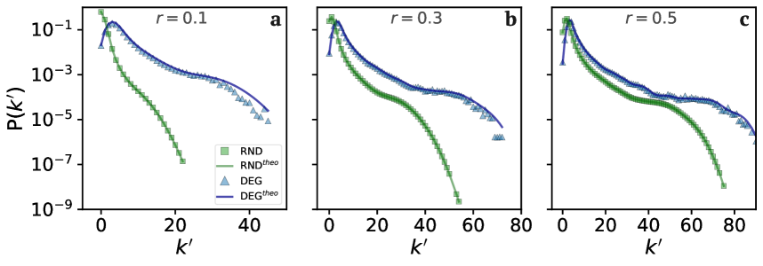
In Supplementary Fig. 1 we report the the empirical degree distributions of the subgraph $G^{\prime}$ induced by the random (RND) and degree-based (DEG) CT strategies when considering three different adoption rates $r=0.1,0.3,0.5$, respectively. We considered here an ensemble of configuration model graphs with degree distribution $P(k)\sim k^{-3}$ and $N=10^{4}$ nodes. Notice that the numerical simulations are in perfect agreement with the analytical predictions in Eq. (3) and Eq. (18)

Simulated annealing

The simulated annealing (SA) procedure is commonly used to find the global optimum of a certain cost/energy function. In a SA algorithm, an energy function usually attributes certain values to each configuration of the system. The best configuration, which is the one that optimises the energy function, is usually identified by searching the phase space of the system considering Markov Chain Monte Carlo moves that allow to switch from one configuration to another. In our context, we are interested on finding the maximum of the following cost function:

$$\mathcal{F}(G^{\prime})=\sum_{\ell}\frac{1}{k_{\ell}}\sum_{i}a_{\ell i}\frac{k^{\prime}_{i}}{k_{i}}(k_{i}-1)$$ (19)

Hence, for a given app adoption rate $r$, the SA algorithm tries to find the nodes which provide the maximum value of $\mathcal{F}$ in order to reduce the expected number of secondary infections caused by a single contagion in presence of contact tracing. Each configuration is represented by the couple $\{A,f\}$, where $A$ is set of nodes ID which adopts the CT app in the network, while $f$ is the energy associated with the configuration, i.e., the value computed using Eq. 19.

For a given app adoption rate $r$, we start at time $t=0$ from a random configuration $A_{0}$ and evaluate the corresponding energy $f_{0}$. Then, at each step $t$ of the algorithm, we randomly replace a node $i$ of the set $A_{t-1}$ with a randomly selected node $j$ that does not belong to the same set, i.e. $A_{t}=(A_{t-1}\cup\{j\})\setminus\{i\}$. After calculating the energy $f_{t}$ of the new configuration, we accept it with probability:

$$p=\begin{cases}1&\text{ if }f_{t}>f\\ {\rm e}^{-\frac{f-f_{t}}{T}}&\text{otherwise}\end{cases}$$

where $T$ has the role of temperature in the simulated annealing procedure. In particular, the initial temperature for the simulations was set to $T_{max}=1$ and in every step it was reduced by $\delta T$ until $T_{min}=0.01$ was reached. A step of $\delta T=10^{-7}$ was used for all our numerical simulations.

Supplementary Note 2 Contact tracing strategies based on local information

We report in Supplementary Table 1 the real-world networks analysed in the main manuscript along with the thresholds values used for filtering nodes or edges in the networks and basic statistics (resulting number of nodes and edges). For each of the $84$ unique graphs analysed, we report the thresholds used and the resulting number of links with larger weights.

Network	Thres.	Nodes	Edges	Network	Thres.	Nodes	Edges	Network	Thres.	Nodes	Edges
contacts-Hospital	240 sec.	67	291	contacts-Hospital	360 sec.	63	228	highschool-2011	240 sec.	117	332
highschool-2011	360 sec.	111	252	highschool-2012	240 sec.	171	496	highschool-2012	360 sec.	158	372
gall-2009-04-28	0 sec.	190	703	gall-2009-04-28	20 sec.	61	127	gall-2009-04-29	0 sec.	198	736
gall-2009-04-29	20 sec.	112	231	gall-2009-04-30	0 sec.	144	486	gall-2009-04-30	20 sec.	59	132
gall-2009-05-01	0 sec.	201	558	gall-2009-05-01	20 sec.	37	60	gall-2009-05-02	0 sec.	213	966
gall-2009-05-02	20 sec.	89	163	gall-2009-05-03	0 sec.	305	1847	gall-2009-05-03	20 sec.	211	513
gall-2009-05-05	0 sec.	78	147	gall-2009-05-05	20 sec.	18	26	gall-2009-05-06	0 sec.	176	745
gall-2009-05-06	20 sec.	37	65	gall-2009-05-07	0 sec.	194	801	gall-2009-05-07	20 sec.	72	204
gall-2009-05-09	0 sec.	216	993	gall-2009-05-09	20 sec.	156	312	gall-2009-05-10	0 sec.	168	625
gall-2009-05-10	20 sec.	138	242	gall-2009-05-12	0 sec.	56	114	gall-2009-05-12	20 sec.	11	15
gall-2009-05-13	0 sec.	166	590	gall-2009-05-13	20 sec.	58	82	gall-2009-05-14	0 sec.	132	620
gall-2009-05-14	20 sec.	54	134	gall-2009-05-15	0 sec.	241	1301	gall-2009-05-15	20 sec.	127	334
gall-2009-05-16	0 sec.	241	1504	gall-2009-05-16	20 sec.	216	577	gall-2009-05-17	0 sec.	187	1347
gall-2009-05-17	20 sec.	172	470	gall-2009-05-19	0 sec.	49	112	gall-2009-05-19	20 sec.	13	23
gall-2009-05-20	0 sec.	89	507	gall-2009-05-20	20 sec.	75	276	gall-2009-05-21	0 sec.	43	193
gall-2009-05-21	20 sec.	38	107	gall-2009-05-22	0 sec.	131	864	gall-2009-05-22	20 sec.	65	183
gall-2009-05-23	0 sec.	238	1075	gall-2009-05-23	20 sec.	208	396	gall-2009-05-24	0 sec.	31	68
gall-2009-05-24	20 sec.	10	13	gall-2009-05-26	0 sec.	131	513	gall-2009-05-26	20 sec.	57	183
gall-2009-05-27	0 sec.	116	395	gall-2009-05-27	20 sec.	45	118	gall-2009-05-28	0 sec.	141	1054
gall-2009-05-28	20 sec.	100	495	gall-2009-05-29	0 sec.	93	272	gall-2009-05-29	20 sec.	65	132
gall-2009-05-30	0 sec.	127	397	gall-2009-05-30	20 sec.	70	121	gall-2009-05-31	0 sec.	89	267
gall-2009-05-31	20 sec.	22	56	gall-2009-06-02	0 sec.	16	61	gall-2009-06-02	20 sec.	11	41
gall-2009-06-03	0 sec.	62	174	gall-2009-06-03	20 sec.	16	46	gall-2009-06-04	0 sec.	53	382
gall-2009-06-04	20 sec.	37	137	gall-2009-06-05	0 sec.	88	267	gall-2009-06-05	20 sec.	32	56
gall-2009-06-06	0 sec.	142	696	gall-2009-06-06	20 sec.	127	324	gall-2009-06-07	0 sec.	155	563
gall-2009-06-07	20 sec.	113	203	gall-2009-06-09	0 sec.	74	238	gall-2009-06-09	20 sec.	21	70
gall-2009-06-10	0 sec.	35	74	gall-2009-06-10	20 sec.	18	49	gall-2009-06-11	0 sec.	77	161
gall-2009-06-11	20 sec.	13	44	gall-2009-06-12	0 sec.	58	158	gall-2009-06-12	20 sec.	25	101
gall-2009-06-13	0 sec.	102	264	gall-2009-06-13	20 sec.	21	40	gall-2009-06-14	0 sec.	138	433
gall-2009-06-14	20 sec.	105	181	gall-2009-06-16	0 sec.	67	391	gall-2009-06-16	20 sec.	48	198
gall-2009-06-17	0 sec.	72	212	gall-2009-06-17	20 sec.	48	81	gall-2009-06-18	0 sec.	74	275
gall-2009-06-18	20 sec.	23	66	gall-2009-06-19	0 sec.	125	412	gall-2009-06-19	20 sec.	64	112
gall-2009-06-20	0 sec.	149	495	gall-2009-06-20	20 sec.	109	203	gall-2009-06-21	0 sec.	166	676
gall-2009-06-21	20 sec.	123	244	gall-2009-06-23	0 sec.	57	128	gall-2009-06-23	20 sec.	19	31
gall-2009-06-24	0 sec.	79	369	gall-2009-06-24	20 sec.	22	40	gall-2009-06-25	0 sec.	79	321
gall-2009-06-25	20 sec.	31	152	gall-2009-06-26	0 sec.	78	152	gall-2009-06-26	20 sec.	9	13
gall-2009-06-27	0 sec.	35	99	gall-2009-06-27	20 sec.	10	17	gall-2009-06-28	0 sec.	107	397
gall-2009-06-28	20 sec.	35	71	gall-2009-06-30	0 sec.	128	435	gall-2009-06-30	20 sec.	34	55
gall-2009-07-01	0 sec.	167	814	gall-2009-07-01	20 sec.	127	336	gall-2009-07-02	0 sec.	60	180
gall-2009-07-02	20 sec.	21	39	gall-2009-07-03	0 sec.	121	321	gall-2009-07-03	20 sec.	32	60
gall-2009-07-04	0 sec.	127	526	gall-2009-07-04	20 sec.	103	214	gall-2009-07-05	0 sec.	95	314
gall-2009-07-05	20 sec.	30	40	gall-2009-07-07	0 sec.	220	1187	gall-2009-07-07	20 sec.	166	477
gall-2009-07-08	0 sec.	186	820	gall-2009-07-08	20 sec.	159	356	gall-2009-07-09	0 sec.	114	373
gall-2009-07-09	20 sec.	61	121	gall-2009-07-10	0 sec.	157	776	gall-2009-07-10	20 sec.	103	359
gall-2009-07-11	0 sec.	161	673	gall-2009-07-11	20 sec.	102	188	gall-2009-07-12	0 sec.	148	580
gall-2009-07-12	20 sec.	114	215	gall-2009-07-14	0 sec.	275	1633	gall-2009-07-14	20 sec.	195	566
gall-2009-07-15	0 sec.	410	2765	gall-2009-07-15	20 sec.	351	1205	gall-2009-07-16	0 sec.	318	1441
gall-2009-07-16	20 sec.	250	567	gall-2009-07-17	0 sec.	221	1073	gall-2009-07-17	20 sec.	180	405
InVS13	$25\%$	93	967	InVS13	$10\%$	87	391	InVS15	$25\%$	217	4150
InVS15	$10\%$	208	1656	LH10	$25\%$	62	339	LH10	$10\%$	42	116
LyonSchool	$25\%$	240	6637	LyonSchool	$10\%$	225	2654	SFHH	$25\%$	392	17709
SFHH	$10\%$	384	7048	Thiers13	$25\%$	326	10873	Thiers13	$10\%$	69	1223
bt	$25\%$	634	18727	bt	$10\%$	617	7449	call	$25\%$	12	11
call	$10\%$	5	5	enterprise	$25\%$	84	183	enterprise	$10\%$	50	66
Hospital	$25\%$	67	284	Hospital	$10\%$	44	110	sms	$25\%$	19	18
sms	$10\%$	6	5	student	$25\%$	1452	17134	student	$10\%$	956	6670

Supplementary Table 1: Networks analysed and main statistics.

Some of the strategies studied in the main manuscript, such as degree-based targeting, require global and accurate information about the contact network. Unfortunately, this requirement can represent a major challenge in a realistic scenario, as one normally has access only to partial or local information about a node and/or about its immediate neighbours. To mitigate this problem, we explored two decentralised strategies inspired by the friendship paradox in social networks feld1991your_SI ; eom2014generalized_SI and previously considered for efficient vaccination cohen2003efficient_SI ; lelarge2009efficient_SI ; christakis2010social_SI . The paradox is that, on average, in any graph each individual is more likely to have fewer friends than its own friends do, which corresponds to the saying that “your friends are more social than you are”. We leverage this concept to construct node rankings based on a simple “voting” system. In particular, we assume that each node $i$ in the network has the possibility to indicate one of its neighbours as a candidate for app installation. Then, we rank each node $i$ according to the total number of votes $v_{i}$ it received.

Although the voting system requires each node to have access to just local information, it is easy to show that if the graph has no degree-degree correlations, then the number of votes received by a node $i$ is actually proportional to its degree $k_{i}$. In particular if the probability that a node $j$ casts a vote to a neighbour $i$ is $1/k_{j}$, the number of votes received by a node $i$ is given by:

$$v_{i}=k_{i}\sum_{j}A_{ji}\frac{1}{k_{j}},$$ (20)

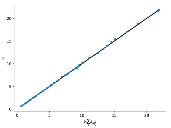
where $a_{ji}$ are the entried of the adjacency matrix of the graph. Despite the number of votes received is proportional to the degree of a node, the inflow also plays a very significant role – similarly to what happens in PageRank – which can lead to some nodes with higher degree actually receiving a smaller number of votes than nodes with a lower degree. In Supplementary Fig. 2 we compare the average number of votes received by each of the nodes in an ensemble of configuration model graphs with degree distribution $P(k)\sim k^{-3}$ and $N=10^{4}$ nodes and the theoretical prediction provide by Eq. (20). The agreement between the simulations and the prediction is perfect, and confirms that indeed the number of votes received by a node is somehow proportional to its degree.

Supplementary Figure 2: Comparison between the votes received by a node and the theoretical prediction when each node casts a single vote. We considered an ensemble of configuration model graphs with degree distribution $P(k)\sim k^{-3}$ and $N=10^{4}$ nodes. The votes received, and the theoretical prediction, have been averaged over all the nodes with the same degree and the black line indicates a perfect match between both.

The assumption that individuals will install the CT app if they are directly targeted, and with probability equal to 1, is rather simplistic and difficult to achieve in real-world systems. Thus, we also explored how effective the mitigation of an epidemic would be when instead of following a strict adoption based on rankings, a node $i$ has a certain probability $\sigma_{i}$ to adopt the app, which depends on the number of votes it has received. One of the simplest approaches to model the adoption of technologies is based on the usage of sigmoid adoption functions stoneman1981intra_SI ; button1993modelling_SI ; tsur1990dynamic_SI in the form:

$$\sigma_{i}(v_{i},a)=\frac{1}{1+\exp(-a(v_{i}-\langle v\rangle))}$$ (21)

where $\langle v\rangle$ is the average number of votes received by nodes in a given realisation, $v_{i}$ is the number of votes received by node $i$, and $a$ tunes the intensity of the sigmoid. In our simulations we considered either $a=1$ or $a=5$.

It is important to note that the function $\sigma_{i}(v,a)$ needs to be properly normalised by $\sum_{i}\sigma_{i}(v_{i},a)$ to obtain a probability function. In Supplementary Fig. 3(a-c) and (d-f), we report the temporal evolution of the number of infected individuals $I(t)$ for the recommendation-based strategy, respectively for the high school and the workplace network analysed in the main manuscript.

Supplementary Figure 3: Impact of CT strategy and adoption rate on the epidemic trajectory in real-world networks. The evolution of the disease in a SIR model with contact tracing depends heavily on the adoption rate and on the strategy considered to select the nodes with CT apps. Here, we show the results on two real-world systems, namely, the high-resolution face-to-face contact data recorded for a high school (a-c) and a workplace network (d-f). The strategies analysed are the recommendation-based (a,d), the sigmoids $\sigma_{i}(v_{i},a=1)$ (b,e), and $\sigma_{i}(v_{i},a=5)$ (c,f). For these simulations we set $\beta=0.1$ and $\mu=0.05$.

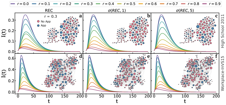
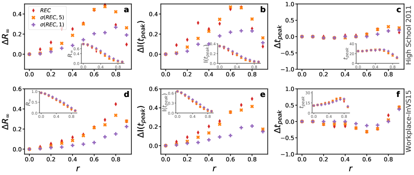
In the high school network we observe a more drastic reduction of cases and larger difference between the strategies as the level of app adoption increases. Furthermore, even though the mitigation effect with the sigmoids is less pronounced than the best case scenarios relying on global information, we still observe a drastic reduction when compared to the random case. In particular, to obtain a strong decrease in the total number of infected individuals we need to consider an adoption rate $r$ above $0.5$. To complement the previous results, Fig. 4 displays the relative improvement over RND for the recommendation-based strategy and the two sigmoids as a function of $r$ for the same two networks. In particular, we focus on the total number $R_{\infty}$ of people who got the disease, the maximum number $I(t_{\rm peak})$ of infected across the duration of the epidemic, and the time $t_{\rm peak}$ at which that number is achieved. Remarkably, for the high school network there are no strong differences in performance between $\sigma_{i}(v_{i},a=5)$ and an assignment based on the ranking of votes received. Finally, the position of the peak does not seem heavily affected by the sigmoid strategies, so that there is still a visible shift of the epidemic peak towards the left for high values of $r$ in the high school network.

Supplementary Figure 4: Comparison of epidemic indicators under different CT strategies. Relative decrease with respect to random installations of the total number of recovered $R_{\infty}$, height of the infection peak $I(t_{\rm peak})$ and position of the peak $t_{\rm peak}$ for the recommendation-based, the sigmoids $\sigma_{i}(v_{i},a=1)$, and $\sigma_{i}(v_{i},a=5)$ installation strategies in the high school (a-c) and workplace networks (d-f). The inset of each panel reports the plot of the raw variable, respectively $R_{\infty}$ (panel a and d), $I(t_{\rm peak})$ (panel b and e) and $t_{\rm peak}$ (panel c and f).

Supplementary Figure 5: Correlations with network structural measures and performance of CT strategies to mitigate an epidemic. For the 168 real-world contact networks analysed, panels (a-c) report the correlation ($R^{2}$) between the epidemiological indicators $\Delta R^{REC}_{\infty}$ (a), $\Delta I^{REC}(t_{\rm peak})$ (b) and $\Delta t^{REC}_{\rm peak}$ (c) and the network density (red), the global efficiency (blue), the rich club coefficient (purple) and the number of maximal cliques (orange) for different values of $r$. All measures were computed considering the full graphs. In panels (d-f), we report the distribution of minimum adoption ratios $r^{*}$ needed to produce a $10\%$ (d), $30\%$ (e) and $50\%$ (f) for the REC (red) and RND (green) strategies. Overall, the REC strategy performs better than RND and requires lower adoption ratios to produce an equivalent reduction of the peak.

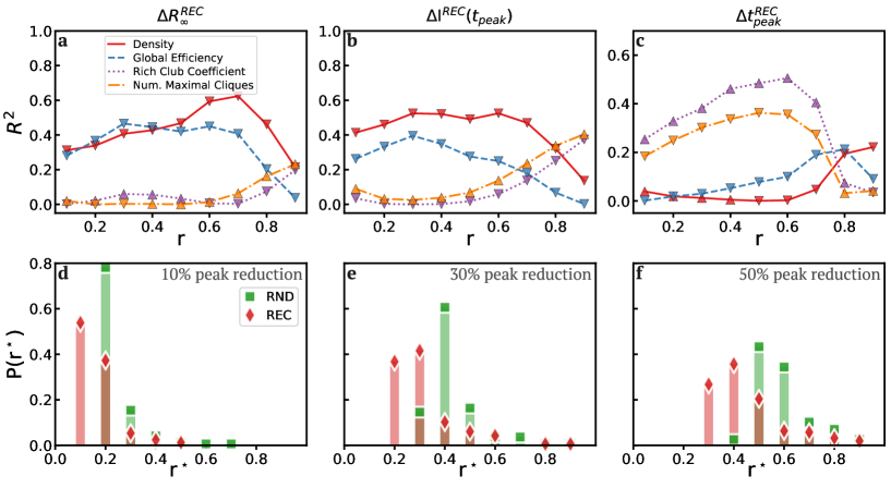
In the following, we refer to the local strategy based on the number of votes $v$ received by a node at the recommendation-based strategy (REC). Considering the 168 networks, Supplementary Fig. 5(a-c) reports the results with the correlations between the epidemiological indicators $\Delta R^{REC}_{\infty}$, $\Delta I^{REC}(t_{\rm peak})$ and $\Delta t^{REC}_{\rm peak}$ and structural measures as a function of the adoption rate $r$. Overall, for low/moderate values of $r$, the performance of the REC strategy – measured by $\Delta R^{REC}_{\infty}$ and $\Delta I^{REC}(t_{\rm peak})$ – displays a moderate correlation only with the density and global efficiency of the contact networks. Conversely, the rich club coefficient and number of maximal cliques show a higher correlation only when considering $\Delta t^{REC}_{\rm peak}$. As done for the DTI, we have also compared how the REC strategy is able to mitigate $I(t_{\rm peak})$ when compared to RND, as can be seen in Supplementary Fig. 5(d-f) where we report the distribution of $r^{*}$ needed for a reduction of of 10%, 30% and 50%, respectively.

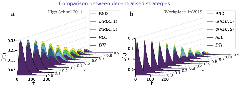
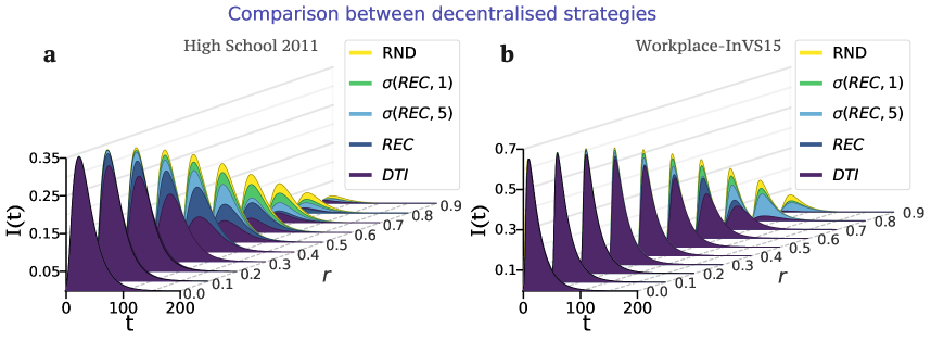
Finally, to compare all the different decentralised CT strategies presented in this work, we report in Supplementary Fig. 6 the epidemic trajectory for the two real-world systems analysed in the main manuscript when considering different CT adoption rates $r$. Overall, $DTI$ is the best performing decentralised strategy, which provides a significant reduction with respect to the random case both in terms of the evolution of the epidemic spreading and for the height of the peak even for low values of installation rate $r$. Such effect is notably visible in the high school network.

Supplementary Figure 6: Mitigation of the epidemic trajectories using decentralised CT strategies. We report the epidemic trajectory when considering different decentralised CT strategies and levels of app adoption $r$ for the two real-world systems considered in the main text. Overall, the CT decentralised strategies consistently lead to a significant reduction of the epidemic trajectory with respect to the random case even for small values installation rate $r$, with $DTI$ being the best-performing strategy.

Supplementary Note 3 SIR model with maximum delay

The SIR model with the ideal contact tracing presented in the main manuscript is based on the assumption that any susceptible node with CT app installed is immediately quarantined (recovered) as soon as one of their contacts with CT app installed gets infected. However, such assumption seems too simplistic when applied to real-world systems. Indeed, people may receive the app notification after several hours/days from an infectious contact, or worse, they may ignore the app notification and continue to have contacts with their acquaintances until they develop symptoms.

As a result, in this section we report the results obtained when considering a different variant of the SIR model $-SIR_{d}-$ which accounts for the maximum delay in self-isolation, so that the neighbours of an infected node only get recovered if an infection event takes place. In other words, if a node $i$ and its neighbour $j$ have both the contact tracing app installed, $j$ will only become recovered if $i$ succeeds into infecting $j$. This mimics the fact that people are in general unwilling to move into self-isolation if they have no symptoms, and represents the maximum possible delay between a positive test and self-isolation of it contacts.

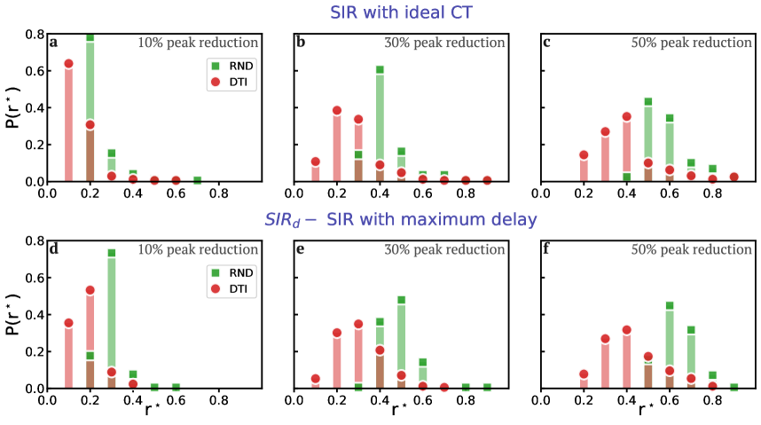
To compare the two SIR variants across the 168 real-world networks analysed in the main manuscript, we report in Supplementary Fig. 7 the RND and DTI distributions of app installation rates $r^{*}$ required to respectively observe a 10, 30, 50% peak reduction with respect to having no contact tracing in place. Interestingly, also when considering the $SIR_{d}$ model, the DTI strategy consistently performs better than the RND. However, all things being equal, on average we need slightly higher CT adoption rates $r$ to achieve similar performances in the peak reduction when considering the $SIR_{d}$ model.

Supplementary Figure 7: Performance of CT strategies in mitigating the epidemics for the two variants of the SIR model. For the 168 real-world networks analysed, we report the distribution of app installation ratios $r^{\star}$ required to observe a $10$, $30$, and $50\%$ peak reduction with respect to no contact tracing for the DTI (red) and RND (green) strategies in the SIR model with ideal contact tracing (a-c) and in the SIR model with delay (d-f). Overall, the DTI strategy performs far better than the RND as it requires lower values of $r$ to induce a similar reduction of the peak in both SIR model variants. However, panels (d-f) clearly show that we need slightly higher CT adoption rates $r$ to achieve similar performances in the peak reduction with the $SIR_{d}$ model.

Furthermore, to easily investigate the impact of the contact tracing strategies when considering the $SIR_{d}$ model, we ran our simulations on the same two real-world systems considered in the main manuscript, the high school and workplace networks. In particular, in Supplementary Fig. 8 we report the comparison of three different epidemic indicators for the $SIR_{d}$ model. Overall, the results are in agreement with the one presented in the main manuscript, so that we observe a great improvement of the targeted CT strategies with respect to the random case in all the three epidemic indicators even for low values of adoption rate $r$. However, we need higher adoption rates to reach levels of reduction of total number of infected and infected in the peak similar to the results presented in the main manuscript, at least 10% difference of installation rate respectively.

Supplementary Figure 8: Comparison of epidemic indicators under different CT strategies for the SIR model with delay. Relative decrease with respect to random installations of the total number of recovered $R_{\infty}$, height of the infection peak $I(t_{\rm peak})$ and position of the peak $t_{\rm peak}$ for DTI, DEG, and SA targeted installation when considering the SIR model with delay. For all the three synthetic indicators, the targeted strategies provide a level of reduction similar to the one presented in the main paper, yet achieved with a slightly higher values of adoption rate $r$ (10% increase). The inset of each panel reports the plot of the raw variable, respectively $R_{\infty}$ (panel a and d), $I(t_{\rm peak})$ (panel b and e) and $t_{\rm peak}$ (panel c and f).

Finally, we show that, even in the $SIR_{d}$ model, the decentralised strategies presented in the main paper (DTI) and in the previous sections (REC and variants) allow to obtain a substantial reduction of the epidemic trajectory with respect to the random case. We report in Supplementary Fig. 9 the comparison between the decentralised strategies when considering the $SIR_{d}$ model for the two real-world systems considered in the main manuscript. Remarkably, even for low values of adoption rate $r$ and also when considering the maximum delay model $SIR_{d}$, the decentralised CT strategies provide a consistent reduction in the epidemic trajectory in respect to the random case.

Supplementary Figure 9: Mitigation of the epidemic using decentralised strategies in the SIR model with delay. We report the epidemic trajectory when considering different CT decentralised strategies and levels of adoption rate $r$ for the two real-world systems considered in the main manuscript using the $SIR_{d}$ model. Interestingly, the CT decentralised strategies consistently lead to a significant reduction of the epidemic trajectory with respect to the RND, with $DTI$ being the best-performing strategy.

References

- (1) McKibbin, W. & Fernando, R. The economic impact of covid-19. Economics in the Time of COVID-19 45 (2020).
- (2) McKibbin, W. J. & Fernando, R. The global macroeconomic impacts of covid-19: Seven scenarios (2020).
- (3) Holman, E. A., Thompson, R. R., Garfin, D. R. & Silver, R. C. The unfolding covid-19 pandemic: A probability-based, nationally representative study of mental health in the united states. Science advances 6, eabd5390 (2020).
- (4) Mega, E. R. Covid has killed more than one million people. how many more will die? Nature (2020).
- (5) Perra, N. Non-pharmaceutical interventions during the covid-19 pandemic: A review. Physics Reports (2021). URL https://www.sciencedirect.com/science/article/pii/S0370157321000624.
- (6) Balcan, D. et al. Multiscale mobility networks and the spatial spreading of infectious diseases. Procs. Natl. Acad. Sci. U.S.A. 106, 21484–21489 (2009).
- (7) Riley, S. Large-scale spatial-transmission models of infectious disease. Science 316, 1298–1301 (2007).
- (8) Ferguson, N. M. et al. Strategies for containing an emerging influenza pandemic in southeast asia. Nature 437, 209–214 (2005).
- (9) Colizza, V., Barrat, A., Barthelemy, M., Valleron, A.-J. & Vespignani, A. Modeling the worldwide spread of pandemic influenza: baseline case and containment interventions. PLoS Medicine 4 (2007).
- (10) Pastor-Satorras, R., Castellano, C., Van Mieghem, P. & Vespignani, A. Epidemic processes in complex networks. Rev. Mod. Phys. 87, 925–979 (2015). URL https://link.aps.org/doi/10.1103/RevModPhys.87.925.
- (11) Flaxman, S. et al. Estimating the effects of non-pharmaceutical interventions on covid-19 in europe. Nature 584, 257–261 (2020).
- (12) Cowling, B. J. et al. Impact assessment of non-pharmaceutical interventions against coronavirus disease 2019 and influenza in hong kong: an observational study. The Lancet Public Health (2020).
- (13) Peak, C. M., Childs, L. M., Grad, Y. H. & Buckee, C. O. Comparing nonpharmaceutical interventions for containing emerging epidemics. Proceedings of the National Academy of Sciences 114, 4023–4028 (2017).
- (14) Arenas, A. et al. Modeling the spatiotemporal epidemic spreading of covid-19 and the impact of mobility and social distancing interventions. Physical Review X 10, 041055 (2020).
- (15) Chang, S. et al. Mobility network models of covid-19 explain inequities and inform reopening. Nature 1–8 (2020).
- (16) Di Domenico, L., Pullano, G., Sabbatini, C. E., Boëlle, P.-Y. & Colizza, V. Impact of lockdown on covid-19 epidemic in île-de-france and possible exit strategies. BMC medicine 18, 1–13 (2020).
- (17) Wiersinga, W. J., Rhodes, A., Cheng, A. C., Peacock, S. J. & Prescott, H. C. Pathophysiology, transmission, diagnosis, and treatment of coronavirus disease 2019 (covid-19): a review. Jama 324, 782–793 (2020).
- (18) Haug, N. et al. Ranking the effectiveness of worldwide covid-19 government interventions. Nature human behaviour 4, 1303–1312 (2020).
- (19) Aguilar, J. et al. Impact of urban structure on covid-19 spread. arXiv preprint arXiv:2007.15367 (2020).
- (20) Rodríguez, P. et al. A population-based controlled experiment assessing the epidemiological impact of digital contact tracing. Nature Communications 12, 1–6 (2021).
- (21) Bradshaw, W. J., Alley, E. C., Huggins, J. H., Lloyd, A. L. & Esvelt, K. M. Bidirectional contact tracing could dramatically improve covid-19 control. Nature communications 12, 1–9 (2021).
- (22) Aleta, A. et al. Modelling the impact of testing, contact tracing and household quarantine on second waves of covid-19. Nature Human Behaviour 4, 964–971 (2020).
- (23) Panovska-Griffiths, J. et al. Determining the optimal strategy for reopening schools, the impact of test and trace interventions, and the risk of occurrence of a second covid-19 epidemic wave in the uk: a modelling study. The Lancet Child & Adolescent Health 4, 817–827 (2020).
- (24) Cohen, J. & Kupferschmidt, K. Countries test tactics in ‘war’against covid-19 (2020).
- (25) Abueg, M. et al. Modeling the combined effect of digital exposure notification and non-pharmaceutical interventions on the covid-19 epidemic in washington state. medRxiv (2020).
- (26) Jiang, T. et al. A survey on contact tracing: the latest advancements and challenges. arXiv preprint arXiv:2011.02094 (2020).
- (27) Kerr, C. C. et al. Controlling covid-19 via test-trace-quarantine. medRxiv (2020).
- (28) Kucharski, A. J. et al. Effectiveness of isolation, testing, contact tracing, and physical distancing on reducing transmission of sars-cov-2 in different settings: a mathematical modelling study. The Lancet Infectious Diseases 20, 1151–1160 (2020).
- (29) Smith, L. E. et al. Adherence to the test, trace and isolate system: results from a time series of 21 nationally representative surveys in the uk (the covid-19 rapid survey of adherence to interventions and responses [corsair] study). medRxiv (2020).
- (30) Eames, K. T. & Keeling, M. J. Contact tracing and disease control. Proceedings of the Royal Society of London. Series B: Biological Sciences 270, 2565–2571 (2003).
- (31) Klinkenberg, D., Fraser, C. & Heesterbeek, H. The effectiveness of contact tracing in emerging epidemics. PloS one 1, e12 (2006).
- (32) Kretzschmar, M. E. et al. Impact of delays on effectiveness of contact tracing strategies for covid-19: a modelling study. The Lancet Public Health 5, e452–e459 (2020).
- (33) Ferretti, L. et al. Quantifying sars-cov-2 transmission suggests epidemic control with digital contact tracing. Science 368 (2020).
- (34) Keeling, M. J., Hollingsworth, T. D. & Read, J. M. Efficacy of contact tracing for the containment of the 2019 novel coronavirus (covid-19). J Epidemiol Community Health 74, 861–866 (2020).
- (35) Park, Y. J. et al. Contact tracing during coronavirus disease outbreak, south korea, 2020. Emerging infectious diseases 26, 2465–2468 (2020).
- (36) Barrat, A., Cattuto, C., Kivelä, M., Lehmann, S. & Saramäki, J. Effect of manual and digital contact tracing on covid-19 outbreaks: a study on empirical contact data. MedRxiv (2020).
- (37) Reyna-Lara, A. et al. Virus spread versus contact tracing: two competing contagion processes. arXiv preprint arXiv:2010.01867 (2020).
- (38) Kryven, I. & Stegehuis, C. Contact tracing in configuration models. Journal of Physics: Complexity (2020).
- (39) Bianconi, G., Sun, H., Rapisardi, G. & Arenas, A. A message-passing approach to epidemic tracing and mitigation with apps. arXiv preprint arXiv:2007.05277 (2020).
- (40) Statista.com statistics on Contact-tracing app adoption rates, as of July 2020. https://www.statista.com/statistics/1134669/share-populations-adopted-covid-contact-tracing-apps-countries/ (2020). [Online; accessed 2021-01-27].
- (41) Gómez-Carballa, A., Bello, X., Pardo-Seco, J., Martinón-Torres, F. & Salas, A. Mapping genome variation of sars-cov-2 worldwide highlights the impact of covid-19 super-spreaders. Genome Research 30, 1434–1448 (2020).
- (42) Miller, S. L. et al. Transmission of sars-cov-2 by inhalation of respiratory aerosol in the skagit valley chorale superspreading event. Indoor air (2020).
- (43) DATASETS SocioPatterns.org. http://www.sociopatterns.org/datasets/ (2016). [Online; accessed 2020-09-30].
- (44) Starnini, M., Machens, A., Cattuto, C., Barrat, A. & Pastor-Satorras, R. Immunization strategies for epidemic processes in time-varying contact networks. Journal of theoretical biology 337, 89–100 (2013).
- (45) Vanhems, P. et al. Estimating potential infection transmission routes in hospital wards using wearable proximity sensors. PloS one 8, e73970 (2013).
- (46) Barrat, A., Cattuto, C., Tozzi, A. E., Vanhems, P. & Voirin, N. Measuring contact patterns with wearable sensors: methods, data characteristics and applications to data-driven simulations of infectious diseases. Clinical Microbiology and Infection 20, 10–16 (2014).
- (47) Génois, M. et al. Data on face-to-face contacts in an office building suggest a low-cost vaccination strategy based on community linkers. Network Science 3, 326–347 (2015). URL http://journals.cambridge.org/article_S2050124215000107.
- (48) Génois, M. & Barrat, A. Can co-location be used as a proxy for face-to-face contacts? EPJ Data Science 7, 11 (2018). URL https://doi.org/10.1140/epjds/s13688-018-0140-1.
- (49) Gadár, L., Kosztyán, Z. T., Telcs, A. & Abonyi, J. A multilayer and spatial description of the erasmus mobility network. Scientific Data 7, 1–11 (2020).
- (50) Sapiezynski, P., Stopczynski, A., Lassen, D. D. & Lehmann, S. Interaction data from the copenhagen networks study. Scientific Data 6, 1–10 (2019).
- (51) Jeyanathan, M. et al. Immunological considerations for covid-19 vaccine strategies. Nature Reviews Immunology 1–18 (2020).
- (52) Gozzi, N., Bajardi, P. & Perra, N. The importance of non-pharmaceutical interventions during the covid-19 vaccine rollout. medRxiv (2021).
- (53) Salathé, M. et al. A high-resolution human contact network for infectious disease transmission. Proceedings of the National Academy of Sciences 107, 22020–22025 (2010).
- (54) Isella, L. et al. What’s in a crowd? analysis of face-to-face behavioral networks. Journal of theoretical biology 271, 166–180 (2011).
- (1) Colizza, V., Flammini, A., Serrano, M. A. & Vespignani, A. Detecting rich-club ordering in complex networks. Nature physics 2, 110–115 (2006).
- (2) Latora, V., Nicosia, V. & Russo, G. Complex networks: principles, methods and applications (Cambridge University Press, 2017).
- (3) Newman, M. Networks (Oxford university press, 2018).
- (4) Feld, S. L. Why your friends have more friends than you do. American Journal of Sociology 96, 1464–1477 (1991).
- (5) Eom, Y.-H. & Jo, H.-H. Generalized friendship paradox in complex networks: The case of scientific collaboration. Scientific reports 4, 1–6 (2014).
- (6) Cohen, R., Havlin, S. & Ben-Avraham, D. Efficient immunization strategies for computer networks and populations. Physical review letters 91, 247901 (2003).
- (7) Lelarge, M. Efficient control of epidemics over random networks. ACM SIGMETRICS Performance Evaluation Review 37, 1–12 (2009).
- (8) Christakis, N. A. & Fowler, J. H. Social network sensors for early detection of contagious outbreaks. PloS one 5, e12948 (2010).
- (9) Stoneman, P. Intra-firm diffusion, bayesian learning and profitability. The Economic Journal 91, 375–388 (1981).
- (10) Button, K., Ngoe, N. & Hine, J. Modelling vehicle ownership and use in low income countries. Journal of Transport Economics and Policy 51–67 (1993).
- (11) Tsur, Y., Sternberg, M. & Hochman, E. Dynamic modelling of innovation process adoption with risk aversion and learning. Oxford Economic Papers 42, 336–355 (1990).