Graph Laplacian for image deblurring

Abstract.

Image deblurring is relevant in many fields of science and engineering. To solve this problem, many different approaches have been proposed and among the various methods, variational ones are extremely popular. These approaches are characterized by substituting the original problem with a minimization one where the functional is composed of two terms, a data fidelity term and a regularization term. In this paper we propose, in the classical $\ell^{2}-\ell^{1}$ minimization with the non-negativity constraint of the solution, the use of the graph Laplacian as regularization operator. Firstly, we describe how to construct the graph Laplacian from the observed noisy and blurred image. Once the graph Laplacian has been built, we solve efficiently the proposed minimization problem splitting the convolution operator and the graph Laplacian by the alternating direction method of multipliers (ADMM). Some selected numerical examples show the good performances of the proposed algorithm.

1. Introduction

We are concerned with the solution of the image deblurring problem; see, e.g., [31] for more details on image deblurring. We will assume that the blurring is space-invariant obtaining a linear system of equations

$$A\mathbf{x}=\mathbf{b},$$

where $\mathbf{x}\in{\mathbb{R}}^{N}$ and $\mathbf{b}\in{\mathbb{R}}^{M}$ are samplings of the unknown image to recover and the blurred image, respectively, while $A\in{\mathbb{R}}^{M\times N}$ is a structured matrix (see below) whose singular values decay rapidly and with no significant gap. The discretization process, along with measurement errors, introduces some perturbations in the data, namely $\boldsymbol{\eta}\in{\mathbb{R}}^{M}$ such that $\|\mathbf{b}-\boldsymbol{\eta}\|=\delta$ in the Euclidean norm, leading to the system

$$A\mathbf{x}=\mathbf{b}+\boldsymbol{\eta}=\mathbf{b}^{\delta}.$$

The perturbations $\boldsymbol{\eta}$ are often referred to as noise. Since, in general, $\boldsymbol{\eta}\notin\mathcal{R}(A)$, we would like to solve the least-square problem

(1.1) $$\arg\min_{\mathbf{x}}\left\|A\mathbf{x}-\mathbf{b}^{\delta}\right\|,$$

where $\left\|\cdot\right\|$ is the Euclidean norm. Let $A^{\dagger}$ denote the Moore-Penrose pseudo-inverse of $A$. The naive solution of (1.1), $A^{\dagger}\mathbf{b}^{\delta}$, is usually a poor approximation of the desired solution $\mathbf{x}^{\dagger}=A^{\dagger}\mathbf{b}$; see, e.g., [24, 30] for more details. This is due to the fact that $A$ is severely ill-conditioned and the solution of (1.1) is extremely sensitive to the presence of the noise in the data. To compute an approximation of $\mathbf{x}^{\dagger}$ we need to use regularization methods. These methods aim at reducing the sensitivity mentioned before. One of the most popular regularization method is Tikhonov regularization where the original minimization problem is substituted by another one of the form

(1.2) $$\arg\min_{\mathbf{x}}\left\|A\mathbf{x}-\mathbf{b}^{\delta}\right\|^{2}+\mu\left\|L\mathbf{x}\right\|^{2},$$

where $L\in{\mathbb{R}}^{p\times n}$ is an operator such that $\mathcal{N}(A)\cap\mathcal{N}(L)=\{\mathbf{0}\}$. The matrix $L$ is the so-called regularization operator and its role is to enforce some a-priori knowledge on the reconstruction. If $A$ is the discretization of an integral operator, then usually $L$ is chosen to be a discretization of either the first or the second derivative; see, e.g., [23]. The formulation (1.2) can be extended for a general $\ell_{p}$-norm

(1.3) $$\arg\min_{\mathbf{x}}\left\|A\mathbf{x}-\mathbf{b}^{\delta}\right\|^{2}+\mu\left\|L\mathbf{x}\right\|^{p}_{p},$$

where $\left\|\mathbf{x}\right\|_{p}^{p}=\sum_{i=1}^{n}|x_{i}|^{p}$ for $p>0$. Note that, for $p<1$ the function $\mathbf{x}\mapsto\left\|\mathbf{x}\right\|_{p}$ is not a norm; see, e.g., [32, 36, 14, 16, 12, 25, 21]. In this paper, we consider le graph Laplacian for $L$ in (1.3) with $p=1$. Therefore, our minimization problem is of the form

(1.4) $$\arg\min_{\mathbf{x}\geq 0}\left\|A\mathbf{x}-\mathbf{b}^{\delta}\right\|^{2}+\mu\left\|L\mathbf{x}\right\|_{1},$$

where we have introduced the non-negativity constraint since images cannot attain negative values.

Recently, the graph Laplacian of a network, built from the image itself, has been proposed as regularization operator mainly for image denoising; see. e.g., [39, 34, 40, 35, 37, 44, 42]. In this paper, we build such an operator and use it in (1.4) to reconstruct blurred images. We propose an automated procedure for the construction of an appropriate graph Laplacian and show its performances in some selected numerical examples. We compare the graph Laplacian with the standard Total Variation (TV) operator (see [41]) and show that our proposal can lead to substantial improvements in the quality of the reconstructed images.

This paper is structured as follows: in Section 2 we recall the definition of the Laplacian of a given graph and we construct the one that we use in the following. Section 3 presents our algorithmic proposal for the solution of (1.4) and Section 4 contains some selected numerical experiments. Finally, we draw some conclusions in Section 5.

1.1. Notation

Discretized images are made by union of several pixels in the plane, and therefore are well represented by nonnegative two-dimensional discrete functions $\mathbf{x}:{\mathbb{R}}^{n_{1}\times n_{2}}\to[0,+\infty)$, $\mathbf{x}(i_{1},i_{2})=x_{i_{1},i_{2}}\in{\mathbb{R}}_{+}$ for $i_{1}=1,\ldots,n_{1},\,i_{2}=1,\ldots,n_{2}$. Clearly, this choice is not unique. Since all the operations and analysis we will produce are invariant with respect to the ordering, for the sake of notational simplicity, we fix $n_{1}=n_{2}=n=\sqrt{N}$ and consider the lexicographic one-dimensional ordering, that is, $(i_{1},i_{2})=:i<j:=(j_{1},j_{2})$ if $i_{1}<j_{1}$ or $i_{1}=j_{1}$ and $i_{2}<j_{2}$. With this choice, an image reads as $\mathbf{x}:{\mathbb{R}}^{N}\to[0,+\infty)$, $\mathbf{x}(i)=x_{i}\in{\mathbb{R}}_{+}$ for $i=1,\ldots,n$, and it is said that $\mathbf{x}$ is the vectorization of a square image.

2. Construction of the graph Laplacian

In this section, we first describe how to construct the Laplacian of a given weighted graph. Then we show how to build an appropriate graph, i.e., a graph whose Laplacian is a “good” regularization operator, given a good approximation of the exact image $\mathbf{x}^{\dagger}$. Finally, we provide an algorithm to construct our $L$ given the problem (1.1).

Given a countable measure space $\left(\mathcal{V},\nu\right)$, where $\nu$ is a positive measure, a symmetric non-negative function $\omega:\mathcal{V}\times\mathcal{V}\to[0,+\infty)$ with zero diagonal is called undirected graph on $\mathcal{V}$. The elements $i,j$ of the set $\mathcal{V}$ are called vertices, and two vertices are connected if $\omega(i,j)>0$. The positive value $w(i,j)$ is called weight associated to the edge $\{i,j\}$; for a modern analytic introduction to graph theory we refer to [33]. If $\mathcal{V}$ is a finite set of $n$ elements, then the graph $\omega$ can be uniquely represented, unless permutations, by the adjacency matrix $\Omega\in{\mathbb{R}}^{N\times N}$

$$\left(\Omega\right)_{i,j}:=\omega(i,j).$$

The linear operator $L_{\omega}:C(\mathcal{V})\to C(\mathcal{V})$, acting on the space $C(\mathcal{V}):=\left\{\mathbf{x}:\mathcal{V}\to{\mathbb{R}}\right\}\simeq{\mathbb{R}}^{N}$ via

$$L_{\omega}\mathbf{x}(i):=\frac{1}{\nu(i)}\sum_{j}\omega(i,j)\left(\mathbf{x}(i)-\mathbf{x}(j)\right)$$

is the graph Laplacian on $C(\mathcal{V})$ associated to the graph $\omega$. It is a symmetric operator with respect to the inner product

$$\langle\mathbf{x},\mathbf{y}\rangle:=\sum_{i}\mathbf{x}(i)\mathbf{y}(i)\nu(i).$$

In many applications, a quite standard choice for the measure $\nu$ is the degree function $\nu=\deg$, defined by

$$\deg(i):=\sum_{j}\omega(i,j).$$

It measures the whole intensity of the weights associated to the vertex $i$. Clearly, this choice makes $L_{\omega}$ not symmetric with respect to the standard Euclidean inner product. A good compromise is to choose the homogeneous measure associated to the Frobenius norm of $\Omega$, i.e., $\nu(i)\equiv\|\Omega\|_{F}$. Let us observe that, writing $D$ as the diagonal matrix such that $(D)_{i,i}=\deg(i)$, then it is easy to check that

$$\|D\|_{1}\leq\|\Omega\|_{F}\leq\|D\|_{2}.$$

Henceforth, we will assume $\nu=\|\Omega\|_{F}$. In matrix form, then the graph Laplacian reads

$$L_{\omega}=\frac{D-\Omega}{\|\Omega\|_{F}}.$$

We wish to construct a graph $\omega$ so that $L_{\omega}$ can be used in (1.4). In principle we would like to construct $\omega$ such that

$$\left\|L_{\omega}\mathbf{x}^{\dagger}\right\|\approx 0.$$

To this aim let $\mathbf{x}^{*}$ be a good approximation of $\mathbf{x}^{\dagger}$. Define $\omega$ as the weighted and undirected graph on $\mathcal{V}$, whose nodes are the pixels of $\mathbf{x}^{\dagger}$ and the weights are defined by

$$\omega(i,j)=\left\{\begin{array}[]{ll}{\rm e}^{-(x^{*}(i)-x^{*}(j))^{2}/\sigma}&\mbox{if }i\neq j\mbox{ and }\left\|i-j\right\|_{\infty}\leq R,\\ 0&\mbox{otherwise,}\end{array}\right.$$

where $\sigma>0$ and $R\in{\mathbb{N}}$ are user-defined parameters. Let us recall that we are using the one-dimensional lexicographic ordering, but the nodes of $\mathcal{V}$ represent points in ${\mathbb{R}}^{2}$. Therefore, $i=(i_{1},i_{2}),j=(j_{1},j_{2})$ and $\|i-j\|_{\infty}=\max\left\{|i_{1}-j_{1}|;|i_{2}-j_{2}|\right\}$. Intuitively, the graph is constructed as follows: we connect two pixels if they are close enough and we weight their connection depending on how similar their values are. In particular, we give a strong connection to pixels that have similar values. The parameter $R$ determines how large is the neighborhood we consider for each pixel and $\sigma$ determines how strong the connection between two close pixels should be.

The construction of this graph, and consequently of the graph Laplacian, in turn depends on the construction of an appropriate approximation $\mathbf{x}^{*}$. As we show in Section 4, if we could choose $\mathbf{x}^{*}=\mathbf{x}^{\dagger}$ we would obtain an almost optimal result. However, this is not possible in realistic scenarios. Therefore, we wish to provide a practical way to determine a good enough $\mathbf{x}^{*}$ in a totally automatic way. To compute $\mathbf{x}^{*}$ we propose to solve (1.2) with a regularization operator defined as follows. Let $L_{1}\in{\mathbb{R}}^{n\times n}$ be

$$L_{1}=\begin{bmatrix}-1&1\\ &-1&1\\ &&\ddots&\ddots\\ &&&-1&1\\ 1&&&&-1\end{bmatrix},$$

i.e., $L_{1}$ is a discretization of the first derivative with periodic boundary conditions (BCs). Let $I_{n}$ be the identity matrix of order $n$, we define $L_{\rm TV}$ by

(2.1) $$L_{\rm TV}=\begin{bmatrix}L_{1}\otimes I_{n}\\ I_{n}\otimes L_{1}\end{bmatrix}\in{\mathbb{R}}^{2N\times N}.$$

Note that $L_{\rm TV}$ is an extremely sparse matrix formed by two Block Circulant with Circulant Blocks (BCCB) matrices stacked one over the other. Therefore, matrix-vector products involving $L_{\rm TV}$ can be performed extremely cheaply (in particular, the flop count is $O(N)$) and $L^{T}_{\rm TV}L_{\rm TV}$ is a BCCB matrix. We exploit the latter property below.

To simplify the computations we impose periodic BCs to the matrix $A$. Thanks to this choice, $A$ is a BCCB matrix; see [31] for more details. We recall that BCCB matrices are diagonalized by the two-dimensional Fourier matrix. Let $F_{1}\in{\mathbb{R}}^{n\times n}$ be the Fourier matrix, i.e., $(F_{1})_{j,k}={\rm e}^{2\pi\iota(j-1)(k-1)/n}$ with $\iota^{2}=-1$, then the two-dimensional Fourier matrix is defined by $F=F_{1}\otimes F_{1}$. Note that matrix-vector products with $F$ and its inverse $F^{*}$ can be performed in $O(N\log N)$ flops with the aid of the fft and ifft algorithms.

As discussed above we wish to solve (1.2) with $L$ described above to determine $L_{\omega}$, i.e., we wish to solve a problem of the form

(2.2) $$\mathbf{x}_{\mu}=\arg\min_{\mathbf{x}}\left\|A\mathbf{x}-\mathbf{b}^{\delta}\right\|^{2}+\mu\left\|L_{\rm TV}\mathbf{x}\right\|^{2},$$

for a certain $\mu>0$. Thanks to the structure of $A$ and $L_{\rm TV}$ this can be solved cheaply for any $\mu$. We can write

(2.3) $$A=F^{*}\Sigma F\quad\mbox{and}\quad L_{\rm TV}=\begin{bmatrix}F^{*}\Lambda_{x}F\\ F^{*}\Lambda_{y}F\end{bmatrix},$$

where $\Sigma$, $\Lambda_{x}$, and $\Lambda_{y}$ are diagonal matrices whose diagonal entries are the eigenvalues of $A$, $L_{1}\otimes I_{n}$, and $I\otimes L_{1}$, respectively. We recall that the eigenvalue of a BCCB matrix $C$ can be computed by $F\mathbf{c}_{1}$, where $\mathbf{c}_{1}$ is the first column of $C$. Assuming that $\mathcal{N}(A)\cap\mathcal{N}(L_{\rm TV})=\{\mathbf{0}\}$ we have that

$$\mathbf{x}_{\mu} =(A^{T}A+\mu L^{T}_{\rm TV}L_{\rm TV})^{-1}A^{T}\mathbf{b}^{\delta}$$

$$=\left(F^{*}\Sigma^{*}FF^{*}\Sigma F+\mu\begin{bmatrix}F^{*}\Lambda_{x}^{*}F&F^{*}\Lambda_{y}^{*}F\end{bmatrix}\begin{bmatrix}F^{*}\Lambda_{x}F\\ F^{*}\Lambda_{y}F\end{bmatrix}\right)^{-1}F^{*}\Sigma^{*}F\mathbf{b}^{\delta}$$

$$=\left(F^{*}\Sigma^{*}\Sigma F+\mu F^{*}(\Lambda_{x}^{*}\Lambda_{x}+\Lambda_{y}^{*}\Lambda_{y})F\right)^{-1}F^{*}\Sigma^{*}F\mathbf{b}^{\delta}$$

$$=F^{*}\left(\Sigma^{*}\Sigma+\mu(\Lambda_{x}^{*}\Lambda_{x}+\Lambda_{y}^{*}\Lambda_{y})\right)^{-1}\Sigma^{*}F\mathbf{b}^{\delta},$$

where the matrix to be inverted is a diagonal matrix. Therefore, $\mathbf{x}_{\mu}$ can be computed for any $\mu$ cheaply.

We now wish to determine in an automatic way the parameter $\mu$. We employ the Generalized Cross Validation (GCV).

Denote by $G(\mu)$ the following function

$$G(\mu)=\frac{\left\|A\mathbf{x}_{\mu}-\mathbf{b}^{\delta}\right\|^{2}}{\mbox{{trace}}(I-A(A^{T}A+\mu L^{T}_{\rm TV}L_{\rm TV})^{-1}A^{T})^{2}}.$$

The GCV parameter is the minimizer of $G(\mu)$, i.e., $\mu_{\rm GCV}=\arg\min_{\mu}G(\mu)$. Given the decomposition (2.3) the value of $G(\mu)$ can be computed in a straightforward way. Introduce the following notation

$$r_{\mu}=\left\|A\mathbf{x}_{\mu}-\mathbf{b}^{\delta}\right\|\quad\mbox{and}\quad t_{\mu}=\mbox{{trace}}(I-A(A^{T}A+\mu L^{T}_{\rm TV}L_{\rm TV})^{-1}A^{T}),$$

therefore, $G(\mu)=r_{\mu}^{2}/t_{\mu}^{2}$. Using the spectral decomposition of $A$ we have

$$r_{\mu} =\left\|A\mathbf{x}_{\mu}-\mathbf{b}^{\delta}\right\|=\left\|F^{*}\Sigma FF^{*}\left(\Sigma^{*}\Sigma+\mu(\Lambda_{x}^{*}\Lambda_{x}+\Lambda_{y}^{*}\Lambda_{y})\right)^{-1}\Sigma^{*}F\mathbf{b}^{\delta}-\mathbf{b}^{\delta}\right\|$$

$$=\left\|\Sigma\left(\Sigma^{*}\Sigma+\mu(\Lambda_{x}^{*}\Lambda_{x}+\Lambda_{y}^{*}\Lambda_{y})\right)^{-1}\Sigma^{*}F\mathbf{b}^{\delta}-F\mathbf{b}^{\delta}\right\|$$

$$=\left\|(\Sigma\Sigma^{*}\left(\Sigma^{*}\Sigma+\mu(\Lambda_{x}^{*}\Lambda_{x}+\Lambda_{y}^{*}\Lambda_{y})\right)^{-1}-I)\widehat{\mathbf{b}^{\delta}}\right\|,$$

where $\widehat{\mathbf{b}^{\delta}}=F\mathbf{b}^{\delta}$. We now move to the computation of $t_{\mu}$

$$t_{\mu} =\mbox{{trace}}(I-A(A^{T}A+\mu L^{T}_{\rm TV}L_{\rm TV})^{-1}A^{T})$$

$$=\mbox{{trace}}(I-F^{*}\Sigma(\Sigma^{*}\Sigma+\mu\left(\Lambda_{x}^{*}\Lambda_{x}+\Lambda_{y}^{*}\Lambda_{y})\right)^{-1}\Sigma^{*}F)$$

$$=\mbox{{trace}}(I-\Sigma\Sigma^{*}(\Sigma^{*}\Sigma+\mu\left(\Lambda_{x}^{*}\Lambda_{x}+\Lambda_{y}^{*}\Lambda_{y})\right)^{-1}).$$

We can observe that, once the decompositions (2.3) and $\widehat{\mathbf{b}^{\delta}}$ have been computed, the evaluation of $G(\mu)$ can be done in $O(N)$ flops. This allows for an extremely fast determination of $\mu_{\rm GCV}$. Finally, we select as $\mathbf{x}^{*}$ the solution of the minimization problem

(2.4) $$\mathbf{x}^{*}=\arg\min_{\mathbf{x}}\left\|A\mathbf{x}-\mathbf{b}^{\delta}\right\|^{2}+\mu_{\rm GCV}\left\|L_{\rm TV}\mathbf{x}\right\|^{2}.$$

Remark 2.1.

If $A$ is constructed with BCs different from the periodic ones it is still possible to compute a fairly accurate approximation of $G(\mu)$ using Krylov subspace methods; see [26, 27, 17, 8].

We summarize the procedure to construct $L_{\omega}$ in Algorithm 1.

Algorithm 1 Construction of $L_{\omega}$ for image deblurring

• Input: $A\in{\mathbb{R}}^{N\times N}$, $\mathbf{b}^{\delta}\in{\mathbb{R}}^{N}$, $R>0$, $\sigma>0$

• Output: $L_{\omega}\in{\mathbb{R}}^{n\times n}$

• Construct $L_{\rm TV}$ as defined in (2.1)

• $\Sigma=\mbox{{diag}}\left(F(A_{(:,1)})\right)$

• $\Lambda_{x}=\mbox{{ diag}}\left(F((L_{\rm TV})_{(:,1:N)})\right)$

• $\Lambda_{y}=\mbox{{ diag}}\left(F((L_{\rm TV})_{(:,N+1:2N)})\right)$

• $\widehat{\mathbf{b}^{\delta}}=F\mathbf{b}^{\delta}$

• $\mu_{\rm GCV}=\arg\min_{\mu}\frac{r_{\mu}^{2}}{t_{\mu}^{2}}$, where

  $$\left\{\begin{array}[]{l}r_{\mu}=\left\|(\Sigma\Sigma^{*}\left(\Sigma^{*}\Sigma+\mu(\Lambda_{x}^{*}\Lambda_{x}+\Lambda_{y}^{*}\Lambda_{y})\right)^{-1}-I)\widehat{\mathbf{b}^{\delta}}\right\|\\ t_{\mu}=\mbox{{trace}}(I-\Sigma\Sigma^{*}(\Sigma^{*}\Sigma+\mu\left(\Lambda_{x}^{*}\Lambda_{x}+\Lambda_{y}^{*}\Lambda_{y})\right)^{-1})\end{array}\right.$$

• $\mathbf{x}^{*}=F^{*}\left(\Sigma^{*}\Sigma+\mu(\Lambda_{x}^{*}\Lambda_{x}+\Lambda_{y}^{*}\Lambda_{y})\right)^{-1}\Sigma^{*}\widehat{\mathbf{b}^{\delta}}$

• Construct $\Omega\in{\mathbb{R}}^{n\times n}$ as

  $$\omega(i,j)=\left\{\begin{array}[]{ll}{\rm e}^{-(x^{*}(i)-x^{*}(j))^{2}/\sigma}&\mbox{if }i\neq j\mbox{ and }\left\|i-j\right\|_{\infty}\leq R,\\ 0&\mbox{else,}\end{array}\right.$$

  with $i$ and $j$ representing two-dimensional indexes, sorted in lexicographic order

• $D=\mbox{{diag}}\{\sum_{j=1}^{n}(\Omega)_{(i,j)}\}$

• $L_{\omega}=\frac{D-\Omega}{\left\|\Omega\right\|_{F}}$

3. Graph Laplacian deblurring

We now describe the non-linear model we employ to compute an approximate solution of (1.1). We consider the graph Laplacian $L_{\omega}$ constructed by Algorithm 1 and we use it in (1.4). Therefore, we wish to solve the following

(3.1) $$\arg\min_{\mathbf{x}\geq 0}\frac{1}{2}\left\|A\mathbf{x}-\mathbf{b}^{\delta}\right\|^{2}+\mu\left\|L_{\omega}\mathbf{x}\right\|_{1}.$$

To solve this problem we use the Alternating Direction Multiplier Method (ADMM); see, e.g., [6] for a recent review. We use ADMM since it allows us to decouple the $\ell^{2}$ and $\ell^{1}$ norms as well as the matrices $A$ and $L_{\omega}$. The latter point is extremely relevant since, as we discuss below, both matrices have exploitable structures, however, they are difficult to exploit together.

We first reformulate (3.1) in an equivalent form

$$\arg\min_{\mathbf{x},\mathbf{y},\mathbf{w},\mathbf{z}}\left\{\frac{1}{2}\left\|A\mathbf{x}-\mathbf{b}^{\delta}\right\|^{2}+\mu\left\|\mathbf{z}\right\|_{1}+\iota_{0}(\mathbf{w}),\mbox{ s.t. }\mathbf{x}=\mathbf{y},\mathbf{x}=\mathbf{w},\mathbf{z}=L_{\omega}\mathbf{y},\right\}$$

or equivalently

(3.2) $$\begin{split}\arg\min_{\mathbf{x},\mathbf{y},\mathbf{w},\mathbf{z}}&\frac{1}{2}\left\|A\mathbf{x}-\mathbf{b}^{\delta}\right\|^{2}+\mu\left\|\mathbf{z}\right\|_{1}+\iota_{0}(\mathbf{w})\\ \mbox{ s.t. }&\begin{bmatrix}I&O\\ O&I\\ I&O\end{bmatrix}\begin{bmatrix}\mathbf{x}\\ \mathbf{z}\end{bmatrix}-\begin{bmatrix}I&O\\ L_{\omega}&O\\ O&I\end{bmatrix}\begin{bmatrix}\mathbf{y}\\ \mathbf{w}\end{bmatrix}=\mathbf{0},\end{split}$$

where $O$ and $\mathbf{0}$ denote the zero matrix and the zero vector, respectively, and $\iota_{0}$ is the indicator function of the nonnegative cone, i.e.,

$$\iota_{0}(\mathbf{x})=\left\{\begin{array}[]{ll}0&\mbox{if }\mathbf{x}\geq 0,\\ +\infty&\mbox{otherwise.}\end{array}\right.$$

We can construct the augmented Lagrangian of (3.2)

$$\mathcal{L}_{\rho}(\mathbf{x},\mathbf{y},\mathbf{w},\mathbf{z};\boldsymbol{\lambda})= \frac{1}{2}\left\|A\mathbf{x}-\mathbf{b}^{\delta}\right\|^{2}+\mu\left\|\mathbf{z}\right\|_{1}+\iota_{0}(\mathbf{w})$$

$$-\left\langle\boldsymbol{\lambda},\begin{bmatrix}I&O\\ O&I\\ I&O\end{bmatrix}\begin{bmatrix}\mathbf{x}\\ \mathbf{z}\end{bmatrix}-\begin{bmatrix}I&O\\ L_{\omega}&O\\ O&I\end{bmatrix}\begin{bmatrix}\mathbf{y}\\ \mathbf{w}\end{bmatrix}\right\rangle$$

$$+\frac{\rho}{2}\left\|\begin{bmatrix}I&O\\ O&I\\ I&O\end{bmatrix}\begin{bmatrix}\mathbf{x}\\ \mathbf{z}\end{bmatrix}-\begin{bmatrix}I&O\\ L_{\omega}&O\\ O&I\end{bmatrix}\begin{bmatrix}\mathbf{y}\\ \mathbf{w}\end{bmatrix}\right\|^{2},$$

where $\rho>0$ is a fixed parameter and $\boldsymbol{\lambda}\in{\mathbb{R}}^{3N}$ is the Lagrangian multiplier. Applying ADMM we get the iterations

$$\left\{\begin{array}[]{l}\vspace*{2mm}\begin{bmatrix}\mathbf{x}^{(k+1)}\\ \mathbf{z}^{(k+1)}\end{bmatrix}=\arg\min_{\mathbf{x},\mathbf{z}}\mathcal{L}_{\rho}(\mathbf{x},\mathbf{y}^{(k)},\mathbf{w}^{(k)},\mathbf{z};\boldsymbol{\lambda}^{(k)}),\\ \begin{bmatrix}\mathbf{y}^{(k+1)}\\ \mathbf{w}^{(k+1)}\end{bmatrix}=\arg\min_{\mathbf{y},\mathbf{w}}\mathcal{L}_{\rho}(\mathbf{x}^{(k+1)},\mathbf{y},\mathbf{w},\mathbf{z}^{(k+1)};\boldsymbol{\lambda}^{(k)}),\\ \boldsymbol{\lambda}^{(k+1)}=\boldsymbol{\lambda}^{(k)}+\rho\left(\begin{bmatrix}I&O\\ O&I\\ I&O\end{bmatrix}\begin{bmatrix}\mathbf{x}^{(k+1)}\\ \mathbf{z}^{(k+1)}\end{bmatrix}-\begin{bmatrix}I&O\\ L_{\omega}&O\\ O&I\end{bmatrix}\begin{bmatrix}\mathbf{y}^{(k+1)}\\ \mathbf{w}^{(k+1)}\end{bmatrix}\right).\end{array}\right.$$

We can write $\boldsymbol{\lambda}=\begin{bmatrix}\boldsymbol{\lambda}_{1}\\ \boldsymbol{\lambda}_{2}\\ \boldsymbol{\lambda}_{3}\end{bmatrix}$ with $\boldsymbol{\lambda}_{j}\in{\mathbb{R}}^{N}$ for $j=1,2,3$. Therefore the minimization problems above decouples and we obtain

All of these minimization problems have a closed form for their solution, namely

$$\left\{\begin{array}[]{l}\mathbf{x}^{(k+1)}=(A^{T}A+2\rho I)^{-1}(A^{T}\mathbf{b}^{\delta}+\rho\mathbf{y}^{(k)}-\boldsymbol{\lambda}^{(k)}_{1}+\rho\mathbf{w}^{(k)}-\boldsymbol{\lambda}^{(k)}_{3}),\\ \mathbf{z}^{(k+1)}=S_{\mu/\rho}\left(L_{\omega}\mathbf{y}^{(k)}-\boldsymbol{\lambda}^{(k)}_{2}/\rho\right),\\ \mathbf{y}^{(k+1)}=(L_{\omega}^{T}L_{\omega}+I)^{-1}(L_{\omega}^{T}(\mathbf{z}^{(k+1)}+\boldsymbol{\lambda}^{(k)}_{2}/\rho)+\mathbf{x}^{(k+1)}+\boldsymbol{\lambda}^{(k)}_{1}/\rho),\\ \mathbf{w}^{(k+1)}=\left(\mathbf{x}^{(k+1)}+\boldsymbol{\lambda}_{3}/\rho\right)_{+},\\ \boldsymbol{\lambda}_{1}^{(k+1)}=\boldsymbol{\lambda}_{1}^{(k)}+\rho(\mathbf{x}^{(k+1)}-\mathbf{y}^{(k+1)}),\\ \boldsymbol{\lambda}_{2}^{(k+1)}=\boldsymbol{\lambda}_{2}^{(k)}+\rho(\mathbf{z}^{(k+1)}-L_{\omega}\mathbf{y}^{(k+1)}),\\ \boldsymbol{\lambda}_{3}^{(k+1)}=\boldsymbol{\lambda}_{3}^{(k)}+\rho(\mathbf{x}^{(k+1)}-\mathbf{w}^{(k+1)}),\end{array}\right.$$

where $S_{\mu}$ denotes the soft-thresholding operator with parameter $\mu$, i.e., $S_{\mu}(\mathbf{x})=\mbox{{sign}}(\mathbf{x})(|\mathbf{x}|-\mu)_{+}$, where the operations are meant element-wise and $(x)_{+}=\max\{x,0\}$ is the metric projection into the nonnegative cone. Note that each iteration requires the solution of two linear systems. The linear system involving $A$ can be easily solved using the fft algorithm if periodic BCs are employed; see above. If other BCs are employed, the structure of the matrix, in general, does not allow to use fast transform for the solution of the system. Nevertheless, this system can be solved by an iterative method using a circulant preconditioner. On the other hand, the solution of linear system with the $L_{\omega}$ matrix can be easily computed using the lsqr algorithm applied to the equivalent least-square problem since the matrix $L_{\omega}$ is extremely sparse.

We would like to briefly discuss the use of the lsqr method for the solution of the system

(3.3) $$(L_{\omega}^{T}L_{\omega}+I)\mathbf{y}^{(k+1)}=(L_{\omega}^{T}(\mathbf{z}^{(k+1)}+\boldsymbol{\lambda}^{(k)}_{2}/\rho)+\mathbf{x}^{(k+1)}+\boldsymbol{\lambda}^{(k)}_{1}/\rho.$$

The linear system of equations (3.3) is equivalent to the least squares problem

(3.4) $$\begin{split}\mathbf{y}^{(k+1)}&=\arg\min_{\mathbf{y}}\left\|\begin{bmatrix}L_{\omega}\\ I\end{bmatrix}\mathbf{y}-\begin{bmatrix}\mathbf{z}^{(k+1)}+\boldsymbol{\lambda}^{(k)}_{2}/\rho\\ \mathbf{x}^{(k+1)}+\boldsymbol{\lambda}^{(k)}_{1}/\rho\end{bmatrix}\right\|^{2}\\ &=\arg\min_{\mathbf{y}}\left\|\widehat{L}\mathbf{y}-\widehat{\mathbf{v}}^{(k)}\right\|^{2}.\end{split}$$

The lsqr algorithm is an iterative method that determines an approximate solution of (3.4) into a Krylov subspace. In particular, at its $j-$th iteration the lsqr algorithm determines a solution of (3.4) in the Krylov subspace $\mathcal{K}_{j}(\widehat{L}^{T}\widehat{L},\widehat{L}^{T}\widehat{\mathbf{v}}^{(k)})$, where

$$\mathcal{K}_{j}(\widehat{L}^{T}\widehat{L},\widehat{L}^{T}\widehat{\mathbf{v}}^{(k)})=\mbox{{span}}\left\{\widehat{L}^{T}\widehat{\mathbf{v}}^{(k)},(\widehat{L}^{T}\widehat{L})\widehat{L}^{T}\widehat{\mathbf{v}}^{(k)},\ldots,(\widehat{L}^{T}\widehat{L})^{j-1}\widehat{L}^{T}\widehat{\mathbf{v}}^{(k)}\right\}.$$

The lsqr method requires one matrix-vector product with $\widehat{L}$ and one with $\widehat{L}^{T}$ at each iteration. Therefore, since $\widehat{L}$ is extremely sparse the flop count per iteration is $O(N)$. Moreover lsqr is mathematically equivalent to the cg method applied to (3.3). However, its implementation is more stable. Nevertheless, the number of iteration required to converge is proportional to $\kappa(\widehat{L})$ which is extremely small; see, e.g., [5] for a discussion on lsqr and cg.

We summarize our approach in Algorithm 2.

Algorithm 2 Graph Laplacian image deblurring

• Input: $A\in{\mathbb{R}}^{N\times N}$, $\mathbf{b}^{\delta}\in{\mathbb{R}}^{N}$, $R>0$, $\sigma>0$, $\rho>0$, $\tau>0$, $K>0$, $\mu>0$

• Output: $\mathbf{x}\in{\mathbb{R}}^{n\times n}$

• Run Algorithm 1 to compute $L_{\omega}$

• $\mathbf{y}^{(0)}=\mathbf{w}^{(0)}=\boldsymbol{\lambda}_{1}^{(0)}=\boldsymbol{\lambda}_{2}^{(0)}=\boldsymbol{\lambda}_{3}^{(0)}=\mathbf{0}$

• for $k=0,\ldots,K$

• $\mathbf{x}^{(k+1)}=(A^{T}A+2\rho I)^{-1}(A^{T}\mathbf{b}^{\delta}+\rho\mathbf{y}^{(k)}-\boldsymbol{\lambda}^{(k)}_{1}+\rho\mathbf{w}^{(k)}-\boldsymbol{\lambda}^{(k)}_{3})$

• $\mathbf{z}^{(k+1)}=S_{\mu/\rho}\left(L_{\omega}\mathbf{y}^{(k)}-\boldsymbol{\lambda}^{(k)}_{2}/\rho\right)$

• $\mathbf{y}^{(k+1)}=(L_{\omega}^{T}L_{\omega}+I)^{-1}(L_{\omega}^{T}(\mathbf{z}^{(k+1)}+\boldsymbol{\lambda}^{(k)}_{2}/\rho)+\mathbf{x}^{(k+1)}+\boldsymbol{\lambda}^{(k)}_{1}/\rho)$

• $\mathbf{w}^{(k+1)}=P_{0}\left(\mathbf{x}^{(k+1)}+\boldsymbol{\lambda}_{3}/\rho\right)$

• $\boldsymbol{\lambda}_{1}^{(k+1)}=\boldsymbol{\lambda}_{1}^{(k)}+\rho(\mathbf{x}^{(k+1)}-\mathbf{y}^{(k+1)})$

• $\boldsymbol{\lambda}_{2}^{(k+1)}=\boldsymbol{\lambda}_{2}^{(k)}+\rho(\mathbf{z}^{(k+1)}-L_{\omega}\mathbf{y}^{(k+1)})$

• $\boldsymbol{\lambda}_{3}^{(k+1)}=\boldsymbol{\lambda}_{3}^{(k)}+\rho(\mathbf{x}^{(k+1)}-\mathbf{w}^{(k+1)})$

• if $k>1\;\&\;\left\|\mathbf{x}^{k+1}-\mathbf{x}^{k}\right\|\leq\tau\left\|\mathbf{x}^{k}\right\|$

• Exit

• end if

• end for

• $\mathbf{x}=\mathbf{x}^{(k+1)}$

Note that since the functional (1.4) is convex we can apply the following classical result on ADMM

Theorem 3.1 (see, e.g., Section 3.2 of Boyd et al. [6]).

With the notation of Algorithm 2 it holds that

1. $\lim_{k\rightarrow\infty}\left\|\begin{bmatrix}I&O\\ O&I\\ I&O\end{bmatrix}\begin{bmatrix}\mathbf{x}^{(k)}\\ \mathbf{z}^{(k)}\end{bmatrix}-\begin{bmatrix}I&O\\ L_{\omega}&O\\ O&I\end{bmatrix}\begin{bmatrix}\mathbf{y}^{(k)}\\ \mathbf{w}^{(k)}\end{bmatrix}\right\|=0$, i.e., the iterates approach feasibility as $k\rightarrow\infty$;

2. $\lim_{k\rightarrow\infty}\frac{1}{2}\left\|A\mathbf{x}^{(k)}-\mathbf{b}^{\delta}\right\|^{2}+\mu\left\|\mathbf{z}^{(k)}\right\|_{1}+\iota_{0}(\mathbf{w}^{(k)})=p^{*}$, where $p^{*}$ is the minimum of (3.1);

3. $\lim_{k\rightarrow\infty}\boldsymbol{\lambda}_{k}=\boldsymbol{\lambda}^{*}$, where $\boldsymbol{\lambda}^{*}$ is a dual optimal point, i.e., a saddle point of $L_{0}$.

Remark 3.2.

ADMM can be slow to converge in certain scenarios. It is not in the scope of this paper to propose a fast algorithm for the solution of (3.1). Rather we wish to show the potentiality of $L_{\omega}$ as a regularization operator. Nevertheless, it is possible to accelerate the convergence of ADMM by extrapolation methods to improve the convergence rate of ADMM; see, e.g., [9, 29].

4. Numerical Examples

We now report some selected numerical examples to show the performances of the proposed method. We are particularly interested in showing that the graph Laplacian constructed in Algorithm 2 provides better reconstructions than the classical TV approach.

We compare the results obtained using $L=L_{\rm TV}$ and $L=L_{\omega}$ in (1.4) with the solution $\mathbf{x}^{*}$ computed in line $9$ of Algorithm 2. To compute the solution of (1.4) with $L=L_{\rm TV}$ we use the algorithm described in [22]. Moreover, we want to show the fill potentiality of the proposed approach. To this aim we construct the operator $L_{\omega}$ using the exact image $\mathbf{x}_{\rm true}$ and we denote it by $\widetilde{L}_{\omega}$. Obviously this approach is not feasible in realistic scenarios, nevertheless it allows us to show the full potentiality of the proposed method.

In all our experiments we set the parameters as specified in Table 1. We compare the considered method in terms of accuracy using the Relative Restoration Error (RRE) computed as

$${\rm RRE}(\mathbf{x})=\frac{\left\|\mathbf{x}-\mathbf{x}_{\rm true}\right\|_{2}}{\left\|\mathbf{x}_{\rm true}\right\|_{2}},$$

the Pick Signal to Noise Ration (PSNR), defined by

$${\rm PSNR}(\mathbf{x})=20\log_{10}\left(\frac{Nm}{\left\|\mathbf{x}_{\rm true}\right\|_{2}}\right),$$

where $m$ denotes the maximum value achievable by $\mathbf{x}_{\rm true}$. Moreover, we consider the Structure SIMilarity index (SSIM), constructed in [43]. The definition of the SSIM is extremely involved, here we simply recall that this statistical index measures how structurally similar two images are, in particular, the higher the SSIM the more similar the images are, and its highest achievable value is $1$.

Table 1. Setting of the parameters in Algorithm 2.

Paramter	Value	Description
$R$	$10$	Support of the weight function in the Graph
$\sigma$	$10^{-2}$	Variance of the weight function in the Graph
$\rho$	$10^{-1}$	Augmentation parameter in ADMM
$\tau$	$10^{-4}$	Stopping criterion for ADMM
$K$	$3000$	Maximum number of iterations
$\mu$	Hand-tuned	Regularization parameter in (1.4)

Example 1.

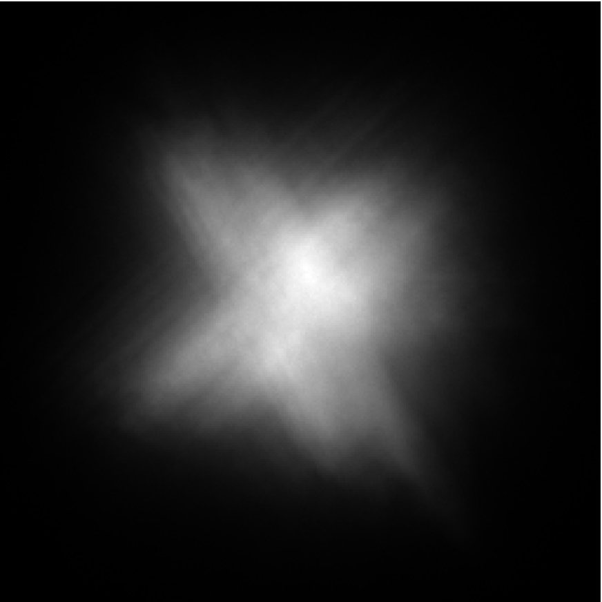
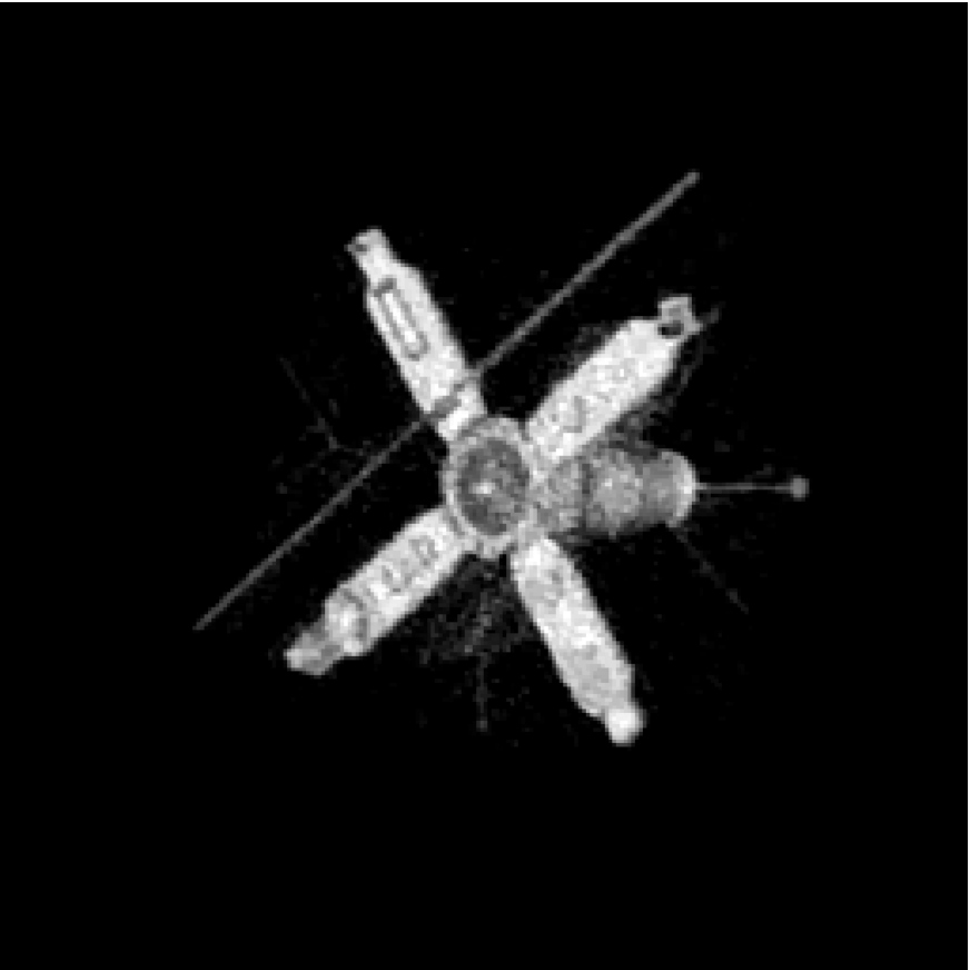
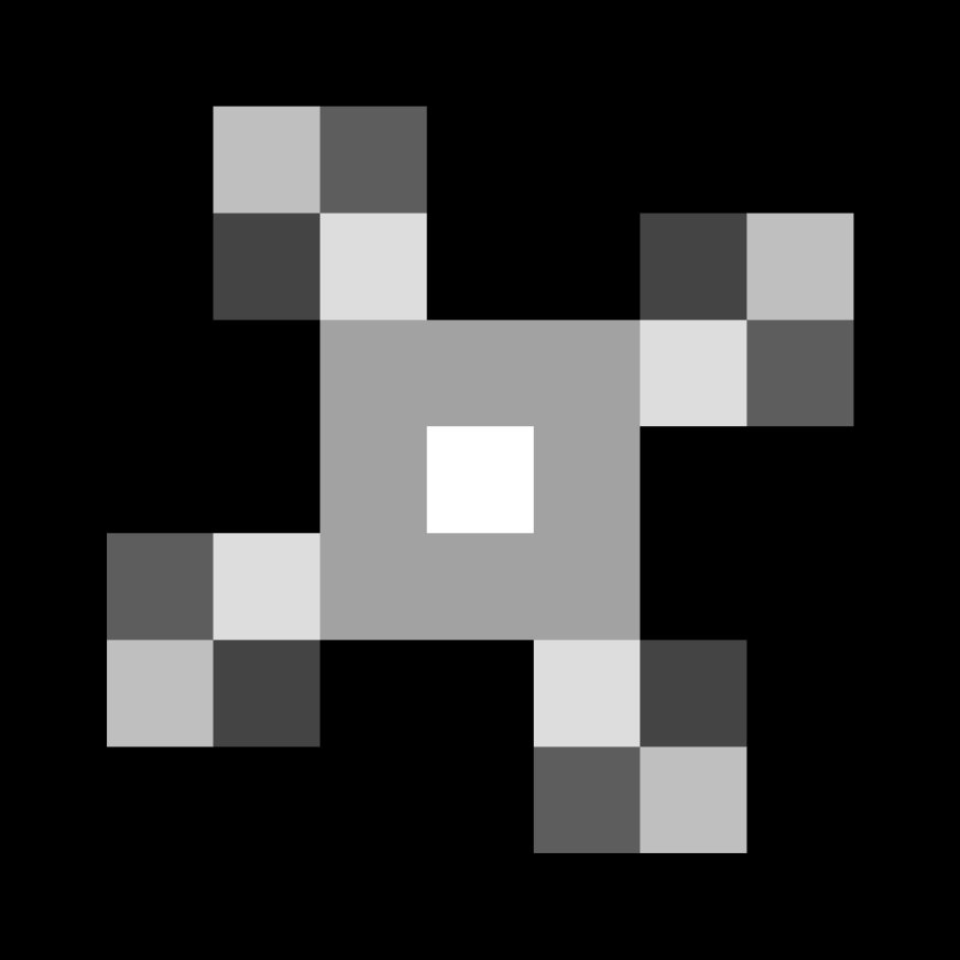
Our first example is the atmosphericBlur50 test case of the RestoreTools toolbox [2]. We report the exact image, the PSF, and the blurred an noisy image in Fig. 2. The norm of the noise, denoted by $\delta$, that corrupts the data is approximately $1\%$ of the norm of the exact right-hand side $\mathbf{b}^{\delta}$.

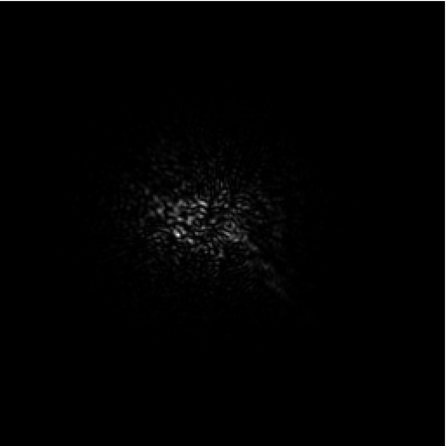
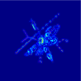
We report the obtained results with the considered methods in Table 2. We can observe that $\ell^{2}-\ell^{1}$ methods provide much more accurate results than the classical Tikhonov method, especially in terms of SSIM. The reconstruction obtained with $L=\widetilde{L}_{\omega}$, i.e., using the graph related to the exact image, is extremely accurate. To validate our model we show in Fig. 1 a visualization of $\left|\widetilde{L}_{\omega}\mathbf{x}^{\dagger}\right|$. We can observe that it is extremely sparse. Therefore, we expect our model to provide accurate reconstructions. However, this approach is not feasible in real scenarios. Nevertheless, we can also observe that using $L=L_{\omega}$ improves the quality of the restoration with respect to the classic TV. This is confirmed by the visual inspection of the reconstructions in Fig. 3. Comparing the reconstructions obtained by the $\ell^{2}-\ell^{1}$ methods we can observe that the choice $L=L_{\rm TV}$ leads to more noisy reconstructions than the ones obtained with the graph Laplacian.

Figure 1. Example 1: Visualization of $\left|\widetilde{L}_{\omega}\mathbf{x}^{\dagger}\right|$ in the jet colormap. The color blue represents the $0$s in the image.

(a)

(b)

(c)

Figure 2. Example 1: (a) True image ($256\times 256$ pixels), (b) PSF ($256\times 256$ pixels), (c) Blurred and noisy image ($256\times 256$ pixels with $\delta\approx 0.01\left\|\mathbf{b}\right\|_{2}$).

(a)

(b)

(c)

Figure 3. Example 1 reconstructions: (a) $\ell^{2}-\ell^{1}$ with $L=L_{\rm TV}$, (b) $\ell^{2}-\ell^{1}$ with $L=L_{\omega}$, (c) $\ell^{2}-\ell^{1}$ with $L=\widetilde{L}_{\omega}$.

Example 2.

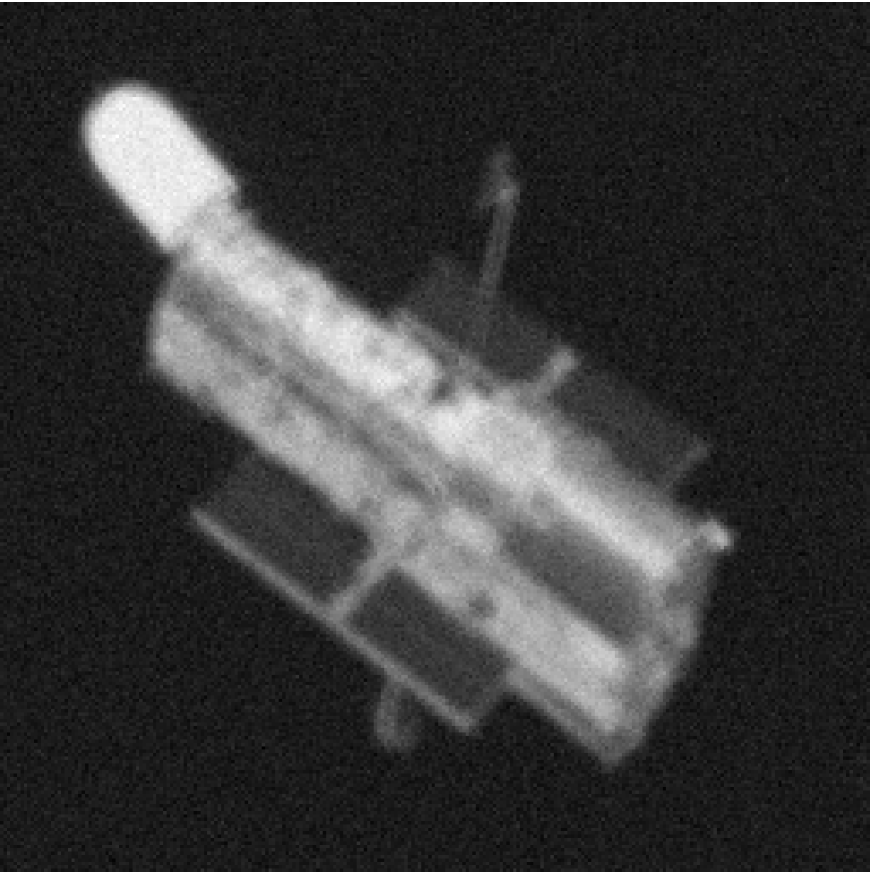
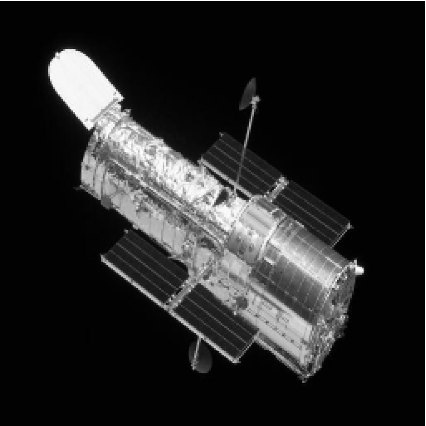
For our second example we consider the Hubble image in Fig. 4(a) and we blur it with the PSF in Fig. 4(b). We then add white Gaussian noise such that $\delta=0.1\left\|\mathbf{b}\right\|_{2}$ obtaining the blurred and noisy image in Fig. 4(c).

We compute approximate solutions with the considered algorithms and report the obtained RRE, PSNR, and SSIM in Table 2. We can observe that our proposal provides the best reconstruction both in terms of RRE (and, therefore of PSNR) and SSIM. This is confirmed by the visual inspection of the reconstructions in Fig. 5. We would like to stress that, similarly as the previous example, the unconstrained Tikhonov method computes extremely noisy reconstructions.

(a)

(b)

(c)

Figure 4. Example 2: (a) True image ($256\times 256$ pixels), (b) PSF ($9\times 9$ pixels), (c) Blurred and noisy image ($256\times 256$ pixels with $\delta=0.1\left\|\mathbf{b}\right\|_{2}$).

(a)

(b)

(c)

Figure 5. Example 2 reconstructions: (a) $\ell^{2}-\ell^{1}$ with $L=L_{\rm TV}$, (b) $\ell^{2}-\ell^{1}$ with $L=L_{\omega}$, (c) $\ell^{2}-\ell^{1}$ with $L=\widetilde{L}_{\omega}$.

Example 3.

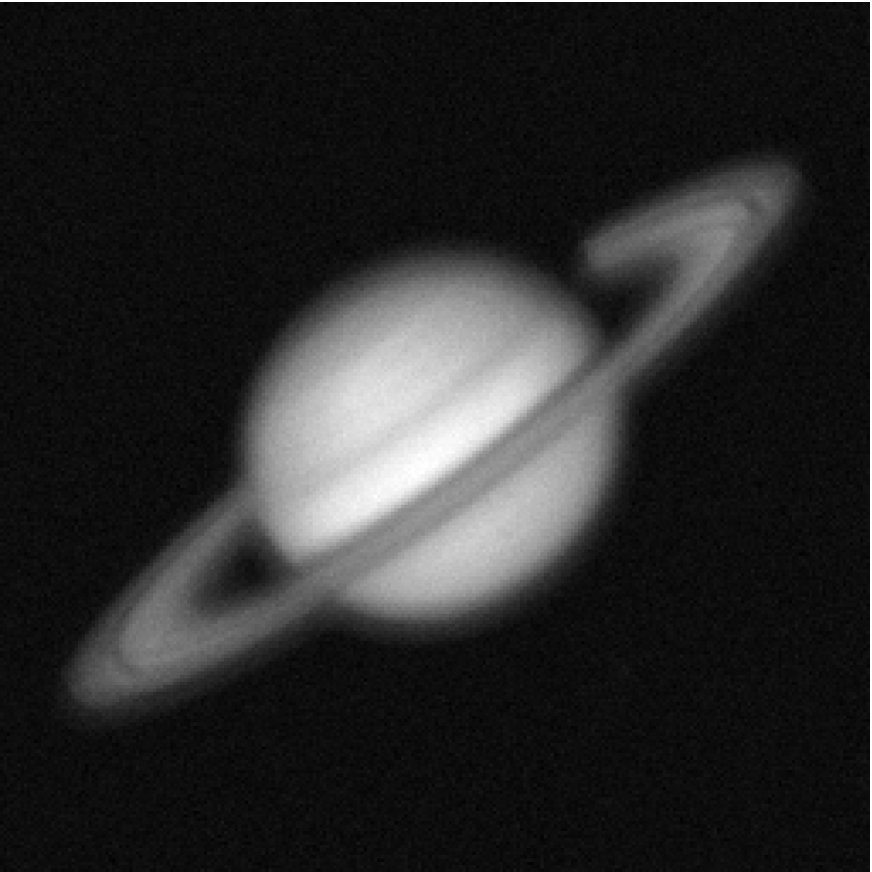
For our third example we consider the Saturn image in Fig. 6(a). We blur it with a non-symmetric PSF (see Fig. 6(b)) and add $5\%$ of white Gaussian noise, i.e., $\delta=0.05\left\|\mathbf{b}\right\|_{2}$ obtaining the image in Fig. 6(c).

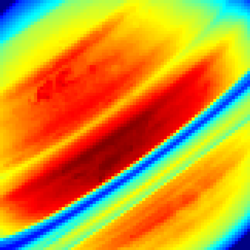
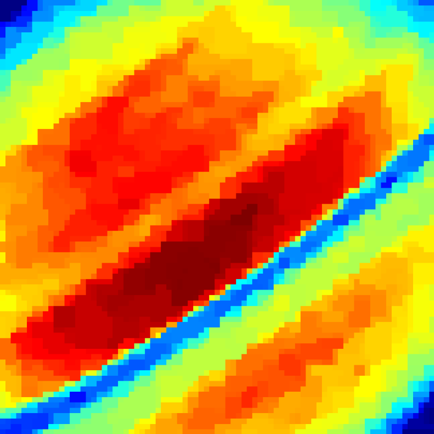
We report in Table 2 the obtained results with the considered algorithms. We can observe that our proposal provides a very accurate reconstruction in terms of RRE and PSNR. However, the SSIM of the computed solution is slightly lower than the one obtained with the standard TV regularization. In Fig. 7 we report all the computed solution. We would like to observe that the reconstruction obtained with the classical TV regularization presents a very heavy stair-case effect while the approximate solution obtained with our proposal avoids this issue. To show this we propose in Fig. 8 blow-ups of the central part of the image of the exact solution and of the reconstructions obtained by TV regularization and our approach. We can observe that the TV reconstruction presents a very heavy stair-case effect that is avoided by our proposal. The solution computed by our method manages to remain extremely sharp, while avoiding any stair-casing.

(a)

(b)

(c)

Figure 6. Example 3: (a) True image ($256\times 256$ pixels), (b) PSF ($17\times 17$ pixels), (c) Blurred and noisy image ($256\times 256$ pixels with $\delta=0.05\left\|\mathbf{b}\right\|_{2}$).

(a)

(b)

(c)

Figure 7. Example 3 reconstructions: (a) $\ell^{2}-\ell^{1}$ with $L=L_{\rm TV}$, (b) $\ell^{2}-\ell^{1}$ with $L=L_{\omega}$, (c) $\ell^{2}-\ell^{1}$ with $L=\widetilde{L}_{\omega}$.

(a)

(b)

(c)

Figure 8. Example 3 blow ups of the exact solution and of two reconstructions in the jet colormap: (a) True solution, (b) $\ell^{2}-\ell^{1}$ with $L=L_{\rm TV}$, (c) $\ell^{2}-\ell^{1}$ with $L=L_{\omega}$.

Example 4.

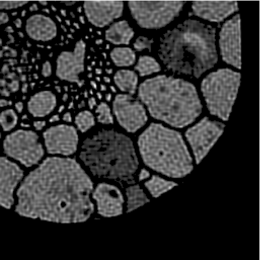
We consider the exact image in Fig. 9(a) and we blur it with an average PSF (see Fig. 9(b)), we add white Gaussian noise so that $\left\|\mathbf{b}-\mathbf{b}^{\delta}\right\|=0.03\left\|\mathbf{b}\right\|$ obtaining Fig. 9(c). We construct the graph Laplacian related to the exact solution $\widetilde{L}_{\omega}$ and deblur the blurred and noisy image with Tikhonov (with $\mu=\mu_{\rm GCV}$) and by minimizing (1.4) with both $L=L_{\rm TV}$ and $L=\widetilde{L}_{\omega}$. We report the results obtained in Table 2. We can observe that the proposed algorithm with the perfect choice of $\widetilde{L}_{\omega}$ largely outperforms the other approaches furnishing a very accurate reconstruction of the proposed image. Moreover, the choice of $L=L_{\omega}$, which we recall that it does not require any a priori information on the exact solution, is still more accurate than the classical TV. This is confirmed by the visual inspection of the reconstructions in Fig. 10.

(a)

(b)

(c)

Figure 9. Example 4: (a) True image ($256\times 256$ pixels), (b) PSF ($12\times 12$ pixels), (c) Blurred and noisy image ($256\times 256$ pixels with $\delta=0.03\left\|\mathbf{b}\right\|_{2}$).

(a)

(b)

(c)

Figure 10. Example 4 reconstructions: (a) $\ell^{2}-\ell^{1}$ with $L=L_{\rm TV}$, (b) $\ell^{2}-\ell^{1}$ with $L=L_{\omega}$, (c) $\ell^{2}-\ell^{1}$ with $L=\widetilde{L}_{\omega}$.

Table 2. Comparison of the RRE, PSNR, and SSIM.

Example	Method	RRE	PSNR	SSIM
Example 1	Tikhonov	$0.22299$	$26.663$	$0.55512$
	$\ell^{2}-\ell^{1}$ with $L=L_{\rm TV}$	$0.19152$	$27.984$	$0.92623$
	$\ell^{2}-\ell^{1}$ with $L=L_{\omega}$	${0.17763}$	${28.638}$	${0.93971}$
	$\ell^{2}-\ell^{1}$ with $L=\widetilde{L}_{\omega}$	$0.083333$	$35.212$	$0.98129$
Example 2	Tikhonov	$0.17352$	$25.735$	$0.55241$
	$\ell^{2}-\ell^{1}$ with $L=L_{\rm TV}$	$0.15492$	$26.720$	$0.80458$
	$\ell^{2}-\ell^{1}$ with $L=L_{\omega}$	$0.14968$	$27.019$	$0.81256$
	$\ell^{2}-\ell^{1}$ with $L=\widetilde{L}_{\omega}$	$0.10096$	$30.439$	$0.89943$
Example 3	Tikhonov	$0.080283$	$33.715$	$0.72254$
	$\ell^{2}-\ell^{1}$ with $L=L_{\rm TV}$	$0.068917$	$35.041$	$0.94873$
	$\ell^{2}-\ell^{1}$ with $L=L_{\omega}$	$0.060094$	$36.231$	$0.94809$
	$\ell^{2}-\ell^{1}$ with $L=\widetilde{L}_{\omega}$	$0.040382$	$39.684$	$0.96489$
Example 4	Tikhonov	$0.16236$	$27.160$	$0.73224$
	$\ell^{2}-\ell^{1}$ with $L=L_{\rm TV}$	$0.15299$	$27.686$	$0.86899$
	$\ell^{2}-\ell^{1}$ with $L=L_{\omega}$	$0.14716$	$28.024$	$0.85765$
	$\ell^{2}-\ell^{1}$ with $L=\widetilde{L}_{\omega}$	$0.085936$	$32.695$	$0.93887$

5. Conclusions

In this paper we have proposed a new regularization operator for $\ell^{2}-\ell^{1}$ minimization. The construction of this operator is automatic and extremely cheap to perform. We have shown that the proposed method outperforms the classical TV approach. Matter of future research include the application of the proposed method to more general inverse problems as well as the integration of the considered method with the $\ell^{p}-\ell^{q}$ minimization proposed in [32, 36, 14, 15, 16, 12] or with iterative regularization methods like, e.g., Linearized Bregman splitting [18, 19, 11, 20, 13] and Iterated Tikhonov with general penalty terms [3, 10, 7, 4]. Another line of future research is the construction of more sophisticated graphs $\omega$ which can better exploit the structure of the given image itself. Such constructions may stem from a PDEs approach; see, e.g., [28, 38, 1].

References

• [1] Adriani, A., Bianchi, D., Serra-Capizzano, S.: Asymptotic Spectra of Large (Grid) Graphs with a Uniform Local Structure (Part I): Theory. Milan J. Math. 87(2), 169–199 (2020)
• [2] Berisha, S., Nagy, J.G.: Iterative methods for image restoration. Tech. rep., Department of Mahtematics and Computer Science, Emory University (2012). http://www.mathcs.emory.edu/~nagy/RestoreTools/IR.pdf
• [3] Bianchi, D., Buccini, A., Donatelli, M., Serra-Capizzano, S.: Iterated fractional Tikhonov regularization. Inverse Problems 31(5), 055005 (2015)
• [4] Bianchi, D., Donatelli, M.: On generalized iterated Tikhonov regularization with operator-dependent seminorms. Electron. Trans. Numer. Anal. 47, 73–99 (2017)
• [5] Björck, Å.: Numerical methods for least squares problems. SIAM (1996)
• [6] Boyd, S., Parikh, N., Chu, E.: Distributed optimization and statistical learning via the alternating direction method of multipliers. Now Publishers Inc (2011)
• [7] Buccini, A.: Regularizing preconditioners by non-stationary iterated tikhonov with general penalty term. Applied Numerical Mathematics 116, 64–81 (2017)
• [8] Buccini, A.: Generalized Cross Validation stopping rule for Iterated Tikhonov regularization. In preparation (2021)
• [9] Buccini, A., Dell’Acqua, P., Donatelli, M.: A general framework for admm acceleration. Numerical Algorithms 85, 829–848 (2020)
• [10] Buccini, A., Donatelli, M., Reichel, L.: Iterated Tikhonov with general penalty term. Accepted on: Numerical Linear Algebra and Applications (2016)
• [11] Buccini, A., Park, Y., Reichel, L.: Numerical aspects of the nonstationary modified linearized Bregman algorithm. Applied Mathematics and Computation 337, 386–398 (2018)
• [12] Buccini, A., Pasha, M., Reichel, L.: Modulus-based iterative methods for constrained pqsuperscript𝑝superscript𝑞\ell^{p}-\ell^{q} minimization. Inverse Problems 36(8), 084001 (2020)
• [13] Buccini, A., Pasha, M., Reichel, L.: Linearized Krylov subspace Bregman iteration with nonnegativity constraint. Numerical Algorithms (In press)
• [14] Buccini, A., Reichel, L.: An 2qsuperscript2superscript𝑞\ell^{2}-\ell^{q} regularization method for large discrete ill-posed problems. Journal of Scientific Computing 78(3), 1526–1549 (2019)
• [15] Buccini, A., Reichel, L.: An 2superscript2\ell^{2}-qsuperscript𝑞\ell^{q} regularization method for large discrete ill-posed problems. Journal of Scientific Computing 78(3), 1526–1549 (2019)
• [16] Buccini, A., Reichel, L.: An psuperscript𝑝\ell^{p}-qsuperscript𝑞\ell^{q} minimization method with cross-validation for the restoration of impulse noise contaminated images. Journal of Computational and Applied Mathematics 375, 112824 (2020)
• [17] Buccini, A., Reichel, L.: Generalized cross validation for psuperscript𝑝\ell^{p}-qsuperscript𝑞\ell^{q} minimization. Under Review (2021)
• [18] Cai, J.F., Osher, S., Shen, Z.: Linearized Bregman iterations for frame-based image deblurring. SIAM Journal on Imaging Sciences 2(1), 226–252 (2009)
• [19] Cai, J.F., Osher, S., Shen, Z.: Split Bregman methods and frame based image restoration. Multiscale Modeling & Simulation 8(2), 337–369 (2009)
• [20] Cai, Y., Donatelli, M., Bianchi, D., Huang, T.Z.: Regularization preconditioners for frame-based image deblurring with reduced boundary artifacts. SIAM Journal on Scientific Computing 38(1), B164–B189 (2016)
• [21] Chan, R.H., Liang, H.X.: Half-quadratic algorithm for psubscript𝑝\ell_{p}-qsubscript𝑞\ell_{q} problems with applications to TV-1subscript1\ell_{1} image restoration and compressive sensing. In: Efficient Algorithms for Global Optimization Methods in Computer Vision, pp. 78–103. Springer (2014)
• [22] Chan, R.H., Tao, M., Yuan, X.: Constrained total variation deblurring models and fast algorithms based on alternating direction method of multipliers. SIAM Journal on imaging Sciences 6(1), 680–697 (2013)
• [23] Donatelli, M., Reichel, L.: Square smoothing regularization matrices with accurate boundary conditions. Journal of Computational and Applied Mathematics 272, 334–349 (2014)
• [24] Engl, H.W., Hanke, M., Neubauer, A.: Regularization of Inverse Problems. Kluwer, Doordrecht (1996)
• [25] Estatico, C., Gratton, S., Lenti, F., Titley-Peloquin, D.: A conjugate gradient like method for p-norm minimization in functional spaces. Numerische Mathematik 137(4), 895–922 (2017)
• [26] Fenu, C., Reichel, L., Rodriguez, G.: GCV for Tikhonov regularization via global Golub-Kahan decomposition. Numerical Linear Algebra with Applications 23(3), 467–484 (2016)
• [27] Fenu, C., Reichel, L., Rodriguez, G., Sadok, H.: GCV for Tikhonov regularization by partial SVD. BIT Numerical Mathematics 57, 1019–1039 (2017)
• [28] Gilboa, G., Osher, S.: On generalized iterated Tikhonov regularization with operator-dependent seminorms. SIAM Multiscale Model. Simul. 7(3), 1005–1028 (2009)
• [29] Goldstein, T., O’Donoghue, B., Setzer, S., Baraniuk, R.: Fast alternating direction optimization methods. SIAM Journal on Imaging Sciences 7(3), 1588–1623 (2014)
• [30] Hansen, P.C.: Rank-deficient and discrete ill-posed problems: numerical aspects of linear inversion. SIAM (1998)
• [31] Hansen, P.C., Nagy, J.G., O’Leary, D.P.: Deblurring Images: Matrices, Spectra, and Filtering. SIAM, Philadelphia (2006)
• [32] Huang, G., Lanza, A., Morigi, S., Reichel, L., Sgallari, F.: Majorization-minimization generalized Krylov subspace methods for psubscript𝑝\ell_{p}-qsubscript𝑞\ell_{q} optimization applied to image restoration. BIT Numerical Mathematics pp. 1–28 (2017)
• [33] Keller, M., Lenz, D., Wojciechowski, R.K.: Graphs and discrete Dirichlet spaces. Grundlehren der mathematischen Wissenschaften: Springer, forthcoming. (2021)
• [34] Kheradmand, A., Milanfar, P.: Motion deblurring with graph laplacian regularization. In: Digital Photography XI, vol. 9404, p. 94040C. International Society for Optics and Photonics (2015)
• [35] Krishnan, D., Fergus, R.: Fast image deconvolution using hyper-laplacian priors. In: Advances in neural information processing systems, pp. 1033–1041 (2009)
• [36] Lanza, A., Morigi, S., Reichel, L., Sgallari, F.: A generalized Krylov subspace method for psubscript𝑝\ell_{p}-qsubscript𝑞\ell_{q} minimization. SIAM Journal on Scientific Computing 37(5), S30–S50 (2015)
• [37] Li, F., Ng, M.K.: Image colorization by using graph bi-laplacian. Advances in Computational Mathematics 45(3), 1521–1549 (2019)
• [38] Lou, Y., Zhang, X., Osher, S., Bertozzi, A.: Image recovery via nonlocal operators. J. Sci. Comput. 42, 185–197 (2010)
• [39] Meyer, F.G., Shen, X.: Perturbation of the eigenvectors of the graph laplacian: Application to image denoising. Applied and Computational Harmonic Analysis 36(2), 326–334 (2014)
• [40] Pang, J., Cheung, G.: Graph laplacian regularization for image denoising: Analysis in the continuous domain. IEEE Transactions on Image Processing 26(4), 1770–1785 (2017)
• [41] Rudin, L.I., Osher, S., Fatemi, E.: Nonlinear total variation based noise removal algorithms. Physica D: nonlinear phenomena 60(1-4), 259–268 (1992)
• [42] Susnjara, A., Perraudin, N., Kressner, D., Vandergheynst, P.: Accelerated filtering on graphs using lanczos method. arXiv preprint arXiv:1509.04537 (2015)
• [43] Wang, Z., Bovik, A.C., Sheikh, H.R., Simoncelli, E.P.: Image quality assessment: from error visibility to structural similarity. IEEE Transactions on Image Processing 13(4), 600–612 (2004)
• [44] Yağan, A.C., Özgen, M.T.: A spectral graph wiener filter in graph fourier domain for improved image denoising. In: 2016 IEEE Global Conference on Signal and Information Processing (GlobalSIP), pp. 450–454. IEEE (2016)