State Entropy Maximization with Random Encoders
for Efficient Exploration

Abstract

Recent exploration methods have proven to be a recipe for improving sample-efficiency in deep reinforcement learning (RL). However, efficient exploration in high-dimensional observation spaces still remains a challenge. This paper presents Random Encoders for Efficient Exploration (RE3), an exploration method that utilizes state entropy as an intrinsic reward. In order to estimate state entropy in environments with high-dimensional observations, we utilize a $k$-nearest neighbor entropy estimator in the low-dimensional representation space of a convolutional encoder. In particular, we find that the state entropy can be estimated in a stable and compute-efficient manner by utilizing a randomly initialized encoder, which is fixed throughout training. Our experiments show that RE3 significantly improves the sample-efficiency of both model-free and model-based RL methods on locomotion and navigation tasks from DeepMind Control Suite and MiniGrid benchmarks. We also show that RE3 allows learning diverse behaviors without extrinsic rewards, effectively improving sample-efficiency in downstream tasks. Source code and videos are available at https://sites.google.com/view/re3-rl.

1 Introduction

Exploration remains one of the main challenges of deep reinforcement learning (RL) in complex environments with high-dimensional observations. Many prior approaches to incentivizing exploration introduce intrinsic rewards based on a measure of state novelty. These include count-based visitation bonuses (Bellemare et al., 2016; Tang et al., 2017; Ostrovski et al., 2017) and prediction errors (Stadie et al., 2015; Houthooft et al., 2016; Pathak et al., 2017; Burda et al., 2019; Pathak et al., 2019; Sekar et al., 2020). By introducing such novelty-based intrinsic rewards, these approaches encourage agents to visit diverse states, but leave unanswered the fundamental question of how to quantify effective exploration in a principled way.

To address this limitation, Lee et al. (2019) and Hazan et al. (2019) proposed that exploration methods should encourage uniform (i.e., maximum entropy) coverage of the state space. For practical state entropy estimation without learning density models, Mutti et al. (2021) estimate state entropy by measuring distances between states and their $k$-nearest neighbors. To extend this approach to high-dimensional environments, recent works (Tao et al., 2020; Badia et al., 2020; Liu & Abbeel, 2021) have proposed to utilize the $k$-nearest neighbor state entropy estimator in a low-dimensional latent representation space. The latent representations are learned by auxiliary tasks such as dynamics learning (Tao et al., 2020), inverse dynamics prediction (Badia et al., 2020), and contrastive learning (Liu & Abbeel, 2021). However, these methods still involve optimizing multiple objectives throughout RL training. Given the added complexity (e.g., hyperparameter tuning), instability, and computational overhead of optimizing auxiliary losses, it is important to ask whether effective state entropy estimation is possible without introducing additional learning procedures.

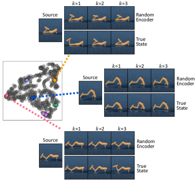
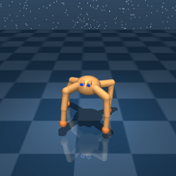
In this paper, we present RE3: Random Encoders for Efficient Exploration, a simple, compute-efficient method for exploration without introducing additional models or representation learning. The key idea of RE3 is to utilize a $k$-nearest neighbor state entropy estimator in the representation space of a randomly initialized encoder, which is fixed throughout training. Our main hypothesis is that a randomly initialized encoder can provide a meaningful representation space for state entropy estimation by exploiting the strong prior of convolutional architectures. Ulyanov et al. (2018) and Caron et al. (2018) found that the structure alone of deep convolutional networks is a powerful inductive bias that allows relevant features to be extracted for tasks such as image generation and classification. In our case, we find that the representation space of a randomly initialized encoder effectively captures information about similarity between states, as shown in Figure 1. Based upon this observation, we propose to maximize a state entropy estimate in the fixed representation space of a randomly initialized encoder.

We highlight the main contributions of this paper below:

• RE3 significantly improves the sample-efficiency of both model-free and model-based RL methods on widely used DeepMind Control Suite (Tassa et al., 2020), MiniGrid (Chevalier-Boisvert et al., 2018), and Atari (Bellemare et al., 2013) benchmarks.

• RE3 encourages exploration without introducing representation learning or additional models, outperforming state entropy maximization schemes that involve representation learning and exploration methods that introduce additional models for exploration (Pathak et al., 2017; Burda et al., 2019).

• RE3 is compute-efficient because it does not require gradient computations and updates for additional representation learning, making it a scalable and practical approach to exploration.

• RE3 allows learning diverse behaviors in environments without extrinsic rewards; we further improve sample-efficiency in downstream tasks by fine-tuning a policy pre-trained with the RE3 objective.

2 Related Work

Exploration in reinforcement learning. Exploration algorithms encourage the RL agent to visit a wide range of states by injecting noise to the action space (Lillicrap et al., 2016) or parameter space (Fortunato et al., 2018; Plappert et al., 2018), maximizing the entropy of the action space (Ziebart, 2010; Haarnoja et al., 2018), and setting diverse goals that guide exploration (Florensa et al., 2018; Nair et al., 2018; Pong et al., 2020; Colas et al., 2019). Another line of exploration algorithms introduce intrinsic rewards proportional to prediction errors (Houthooft et al., 2016; Pathak et al., 2017; Burda et al., 2019; Sekar et al., 2020), and count-based state novelty (Bellemare et al., 2016; Tang et al., 2017; Ostrovski et al., 2017). Our approach differs in that we explicitly encourage the agent to uniformly visit all states by maximizing the entropy of the state distribution, instead of depending on metrics from additional models.

State entropy maximization. Most closely related to our work are methods that maximize the entropy of state distributions. Hazan et al. (2019); Lee et al. (2019) proposed to maximize state entropy estimated by approximating the state density distribution. Instead of approximating complex distributions, Mutti et al. (2021) proposed to maximize a $k$-nearest neighbor state entropy estimate from on-policy transitions. Recent works extend this method to environments with high-dimensional observations. Tao et al. (2020) employ model-based RL techniques to build a representation space for the state entropy estimate that measures similarity in dynamics, and Badia et al. (2020) proposed to measure similarity in the representation space learned by inverse dynamics prediction. The work closest to ours is Liu & Abbeel (2021), which uses off-policy RL algorithms to maximize the $k$-nearest neighbor state entropy estimate in contrastive representation space (Srinivas et al., 2020) for unsupervised pre-training. We instead explore the idea of utilizing a fixed random encoder to obtain a stable entropy estimate without any representation learning.

Figure 1: Visualization of $k$-nearest neighbors of states found by measuring distances in the representation space of a randomly initialized encoder (Random Encoder) and ground-truth state space (True State) on the Hopper environment from DeepMind Control Suite (Tassa et al., 2020). We observe that the representation space of a random encoder effectively captures information about the similarity between states without any representation learning.

Random encoders. Random weights have been utilized in neural networks since their beginnings, most notably in a randomly initialized first layer (Gamba et al., 1961) termed the Gamba perceptron by Minsky & Papert (1969). Moreover, nice properties of random projections are commonly exploited for low-rank approximation (Vempala, 2005; Rahimi & Recht, 2007). These ideas have since been extended to deep convolutional networks, where random weights are surprisingly effective at image generation and restoration (Ulyanov et al., 2018), image classification and detection (Caron et al., 2018), and fast architecture search (Saxe et al., 2011). In natural language processing, Wieting & Kiela (2019) demonstrated that learned sentence embeddings show marginal performance gain over random embeddings. In the context of RL, Gaier & Ha (2019) showed that competitive performance can be achieved by architecture search over random weights without updating weights, and Lee et al. (2020) utilized randomized convolutional neural networks to improve the generalization of deep RL agents. Building on these works, we show that random encoders can also be useful for efficient exploration in environments with high-dimensional observations.

Figure 2: Illustration of our approach. The intrinsic reward for each observation is computed as the distance to its $k$-nearest neighbor, measured between low-dimensional representations obtained from the fixed random encoder. The intrinsic reward is then combined with extrinsic reward from the environment, if present. A separate RL encoder is introduced for a policy that maximizes expected reward.

3 Method

3.1 Preliminaries

We formulate a control task with high-dimensional observations as a partially observable Markov decision process (POMDP; Sutton & Barto 2018; Kaelbling et al. 1998), which is defined as a tuple $\left(\mathcal{O},\mathcal{A},p,r^{\tt{e}},\gamma\right)$. Here, $\mathcal{O}$ is the high-dimensional observation space, $\mathcal{A}$ is the action space, $p\left(o^{\prime}|o_{\leq t},a_{t}\right)$ is the transition dynamics, $r^{\tt{e}}:\mathcal{O}\times\mathcal{A}\rightarrow\mathbb{R}$ is the reward function that maps the current observation and action to a reward $r^{\tt{e}}_{t}=r^{\tt{e}}\left(o_{\leq t},a_{t}\right)$, and $\gamma\in[0,1)$ is the discount factor. By following common practice (Mnih et al., 2015), we reformulate the POMDP as an MDP (Sutton & Barto, 2018) by stacking consecutive observations into a state $s_{t}=\{o_{t},o_{t-1},o_{t-2},...\}$. For simplicity of notation, we redefine the reward function as $r^{\tt{e}}_{t}=r^{\tt{e}}\left(s_{t},a_{t}\right)$. The goal of RL is to learn a policy $\pi(a_{t}|s_{t})$ that maximizes the expected return defined as the total accumulated reward.

$\bm{k}$-nearest neighbor entropy estimator. Let $X$ be a random variable with a probability density function $p$ whose support is a set $\mathcal{X}\subset\mathbb{R}^{q}$. Then its differential entropy is given as $\mathcal{H}(X)=-\mathbb{E}_{x\sim p(x)}[\log p(x)]$. When the distribution $p$ is not available, this quantity can be estimated given $N$ i.i.d realizations of $\{x_{i}\}^{N}_{i=1}$ (Beirlant et al., 1997). However, since it is difficult to estimate $p$ with high-dimensional data, particle-based $k$-nearest neighbors ($k$-NN) entropy estimator (Singh et al., 2003) can be employed:

$$\widehat{\mathcal{H}}^{k}_{N}(X) =\frac{1}{N}\sum^{N}_{i=1}\log\frac{N\cdot||x_{i}-x_{i}^{\text{$k$-NN}}||_{2}^{q}\cdot\widehat{\pi}^{\frac{q}{2}}}{k\cdot\Gamma(\frac{q}{2}+1)}+C_{k}$$ (1)

$$\propto\frac{1}{N}\sum^{N}_{i=1}\log||x_{i}-x_{i}^{\text{$k$-NN}}||_{2},$$ (2)

where $x_{i}^{\text{$k$-NN}}$ is the $k$-NN of $x_{i}$ within a set $\{x_{i}\}_{i=1}^{N}$, $C_{k}=\log k-\Psi(k)$ a bias correction term, $\Psi$ the digamma function, $\Gamma$ the gamma function, $q$ the dimension of $x$, $\widehat{\pi}\approx 3.14159$, and the transition from (1) to (2) always holds for $q>0$.

3.2 Random Encoders for Efficient Exploration

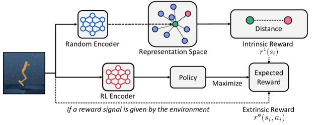
We present Random Encoders for Efficient Exploration (RE3), which encourages exploration in high-dimensional observation spaces by maximizing state entropy. The key idea of RE3 is $k$-nearest neighbor entropy estimation in the low-dimensional representation space of a randomly initialized encoder. To this end, we propose to compute the distance between states in the representation space of a random encoder $f_{\theta}$ whose parameters $\theta$ are randomly initialized and fixed throughout training. The main motivation arises from our observation that distances in the representation space of $f_{\theta}$ are already useful for finding similar states without any representation learning (see Figure 1).

State entropy estimate as intrinsic reward. To define the intrinsic reward proportional to state entropy estimate by utilizing (2), we follow the idea of Liu & Abbeel (2021) that treats each transition as a particle, hence our intrinsic reward is given as follows:

$$r^{\tt{i}}(s_{i}):=\log(||y_{i}-y^{\text{$k$-NN}}_{i}||_{2}+1),$$ (3)

where $y_{i}=f_{\theta}(s_{i})$ is a fixed representation from a random encoder and $y_{i}^{\text{$k$-NN}}$ is the $k$-nearest neighbor of $y_{i}$ within a set of $N$ representations $\{y_{1},y_{2},...,y_{N}\}$. Here, our intuition is that measuring the distance between states in the fixed representation space produces a more stable intrinsic reward as the distance between a given pair of states does not change during training. To compute distances in latent space in a compute-efficient manner, we propose to additionally store low-dimensional representations $y$ in the replay buffer $\mathcal{B}$ during environment interactions. Therefore, we avoid processing high-dimensional states through an encoder for obtaining representations at every RL update. Moreover, we can feasibly compute the distance of $y_{i}$ to all entries $y\in\mathcal{B}$, in contrast to existing approaches that utilize on-policy samples (Mutti et al., 2021), or samples from a minibatch (Liu & Abbeel, 2021). Our scheme enables stable, precise entropy estimation in a compute-efficient manner.

(a) Walker

(b) Hopper

(c) Quadruped

(d) Cheetah

(e) Cartpole

(f) Pendulum

Figure 3: Image observations for visual control tasks from DeepMind Control Suite (Tassa et al., 2020) used in our experiments. The high-dimensionality of these observations necessitates an efficient method for state entropy estimation.

The RE3 objective. We propose to utilize the intrinsic reward $r^{\tt{i}}$ for (a) online RL, where the agent solves target tasks guided by extrinsic reward $r^{\tt{e}}$ from environments, and (b) unsupervised pre-training, where the agent learns to explore the high-dimensional observation space in the absence of extrinsic rewards, i.e., $r^{\tt{e}}=0$. This exploratory policy from pre-training, in turn, can be used to improve the sample-efficiency in downstream tasks by fine-tuning. Formally, we introduce a policy $\pi_{\phi}$, parameterized by $\phi$, that maximizes the expected return $\mathbb{E}_{\pi_{\phi}}\left[\sum^{\infty}_{j=0}\gamma^{j}r^{\tt{total}}_{j}\right]$, where the total reward $r^{\tt{total}}_{j}$ is defined as:

$$r^{\tt{total}}_{j}:=r^{\tt{e}}(s_{j},a_{j})+\beta_{t}\cdot r^{\tt{i}}(s_{j}),$$ (4)

where $\beta_{t}\geq 0$ is a hyperparameter that determines the tradeoff between exploration and exploitation at training timestep $t$. We use the exponential decay schedule for $\beta_{t}$ throughout training to encourage the agent to further focus on extrinsic reward from environments as training proceeds, i.e., $\beta_{t}=\beta_{0}(1-\rho)^{t}$, where $\rho$ is a decay rate. While the proposed intrinsic reward would converge to 0 as more similar states are collected during training, we discover that decaying $\beta_{t}$ empirically stabilizes the performance. We provide the full procedure for RE3 with off-policy RL in Algorithm 1 and on-policy RL in Algorithm 2.

Figure 4: Performance on locomotion tasks from DeepMind Control Suite. RE3 consistently improves the sample-efficiency of RAD and Dreamer. The solid line and shaded regions represent the mean and standard deviation, respectively, across five runs.

Figure 5: We compare state entropy (SE) maximization with RE3 to state entropy maximization schemes that involve representation learning. The solid line and shaded regions represent the mean and standard deviation, respectively, across five runs.

4 Experiments

We designed experiments to answer the following questions:

• Can RE3 improve the sample-efficiency of both model-free and model-based RL algorithms (see Figure 4)?

• How does RE3 compare to state entropy maximization schemes that involve representation learning (see Figure 5) and other exploration schemes that introduce additional models for exploration (see Figure 6)?

• How compute-efficient is RE3 (see Figure 7)?

• Can RE3 further improve the sample-efficiency of off-policy RL algorithms by unsupervised pre-training (see Figure 8 and Figure 9)?

• Can RE3 also improve the sample-efficiency of on-policy RL and off-policy RL in discrete control tasks (see Figure 11 and Figure 13)?

4.1 DeepMind Control Suite Experiments

Setup. To evaluate the sample-efficiency of our method, we compare to Dreamer (Hafner et al., 2020), a state-of-the-art model-based RL method for visual control; and two state-of-the-art model-free RL methods, RAD (Laskin et al., 2020) and DrQ (Kostrikov et al., 2021). For comparison with other exploration methods, we consider RND (Burda et al., 2019) and ICM (Pathak et al., 2017) that introduce additional models for exploration. For RE3 and baseline exploration methods, we use RAD as the underlying model-free RL algorithm. To further demonstrate the applicability of RE3 to model-based RL algorithms, we also consider a combination of Dreamer and RE3. For random encoders, we use convolutional neural networks with the same architecture as underlying RL algorithms, but with randomly initialized parameters fixed during the training. As for the newly introduced hyperparameters, we use $k=3$, $\beta_{0}\in\{0.05,0.25\}$, and $\rho\in\{0.0,0.00001,0.000025\}$. We provide more details in Appendix A. Source code is available at https://sites.google.com/view/re3-rl.

Algorithm 1 RE3: Off-policy RL version

1:  Initialize parameters of random encoder $\theta$, policy $\phi$

2:  Initialize replay buffer $\mathcal{B}\leftarrow\emptyset$

3:  for each timestep $t$ do

4:     // Collect transitions

5:     Collect a transition $\tau_{t}=(s_{t},a_{t},s_{t+1},r^{\tt{e}}_{t})$ from the interaction with the environment using policy $\pi_{\phi}$

6:     Get a fixed representation $y_{t}=f_{\theta}(s_{t})$

7:     $\mathcal{B}\leftarrow\mathcal{B}\cup\{(\tau_{t},y_{t})\}$

8:     // Compute intrinsic reward

9:     Sample random minibatch $\{(\tau_{j},y_{j})\}^{B}_{j=1}\sim\mathcal{B}$

10:     for $j=1$ to $B$ do

11:        Compute the distance $||y_{j}-y||_{2}$ for all representations $y\in\mathcal{B}$ and find the $k$-nearest neighbor $y_{j}^{\text{$k$-NN}}$

12:        Compute $r_{j}^{\tt{i}}\leftarrow\log(||y_{j}-y_{j}^{\text{$k$-NN}}||_{2}+1)$

13:        Update $\beta_{t}\leftarrow\beta_{0}(1-\rho)^{t}$

14:        Let $r^{\tt{total}}_{j}\leftarrow r_{j}^{\tt{e}}+\beta_{t}\cdot r_{j}^{\tt{i}}$

15:     end for

16:     // Update policy

17:     Update $\phi$ with transitions $\{(s_{j},a_{j},s_{j+1},r_{j}^{\tt{total}})\}_{j=1}^{B}$

18:  end for

Figure 6: Performance on locomotion tasks from DeepMind Control Suite. RAD + RE3 outperforms other exploration methods in terms of sample-efficiency. The solid line and shaded regions represent the mean and standard deviation, respectively, across five runs.

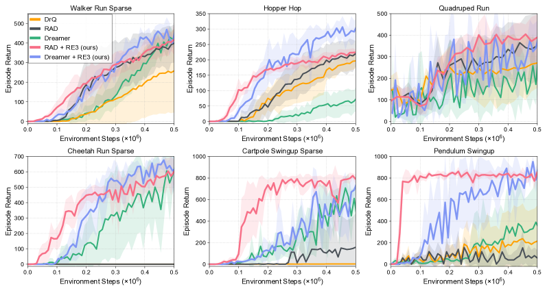
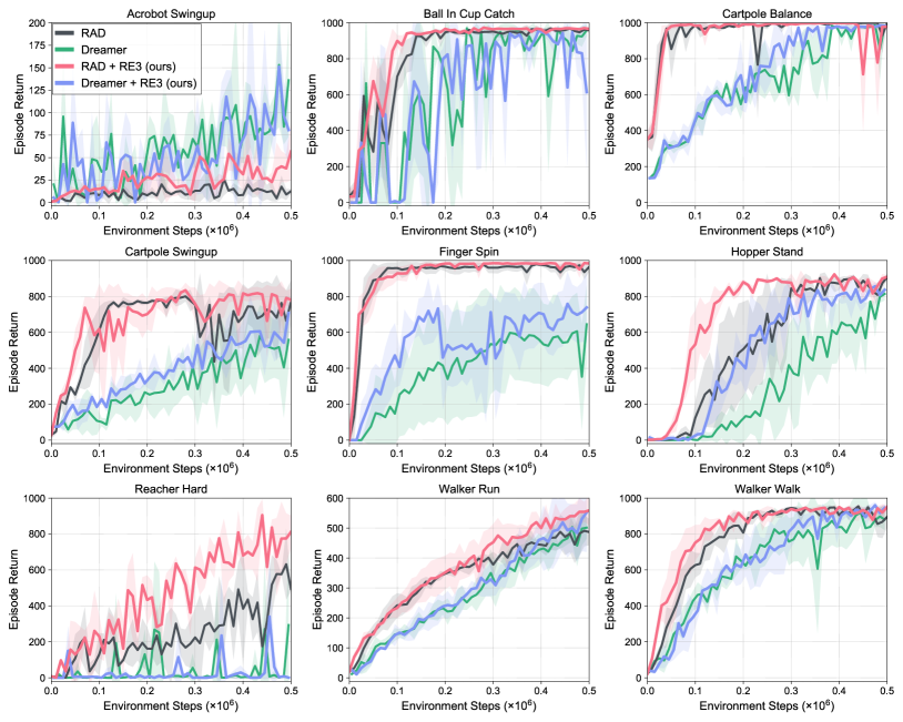
Comparative evaluation. Figure 4 shows that RE3 consistently improves the sample-efficiency of RAD on various tasks. In particular, RAD + RE3 achieves average episode return of 601.6 on Cheetah Run Sparse, where both model-free RL methods RAD and DrQ fail to solve the task. We emphasize that state entropy maximization with RE3 achieves such sample-efficiency with minimal cost due to its simplicity and compute-efficiency. We also observe that Dreamer + RE3 improves the sample-efficiency of Dreamer on most tasks, which demonstrates the applicability of RE3 to both model-free and model-based RL algorithms.

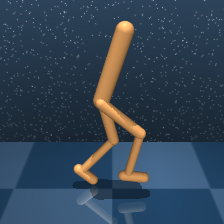
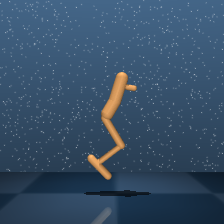
Effects of representation learning. To better grasp how RE3 improves sample-efficiency, we compare to state entropy maximization schemes that involve representation learning in Figure 5. Specifically, we consider a convolutional encoder trained by contrastive learning (RAD + SE w/ Contrastive), inverse dynamics prediction (RAD + SE w/ Inverse dynamics), and a ResNet-50 (He et al., 2016) encoder pre-trained on ImageNet dataset (RAD + SE w/ ImageNet). We found that our method (RAD + SE w/ Random) exhibits better sample-efficiency than approaches that continually update representations throughout training (RAD + SE w/ Contrastive, RAD + SE w/ Inverse dynamics). This demonstrates that utilizing fixed representations helps improve sample-efficiency by enabling stable state entropy estimation throughout training. We also observe that our approach outperforms RAD + SE w/ ImageNet, implying that it is not necessarily beneficial to employ a pre-trained encoder, and fixed random encoders can be effective for state entropy estimation without having been trained on any data. We remark that representations from the pre-trained ImageNet encoder could not be useful for our setup, due to the different visual characteristics of natural images in the ImageNet dataset and image observations in our experiments (see Figure 3 for examples of image observations).

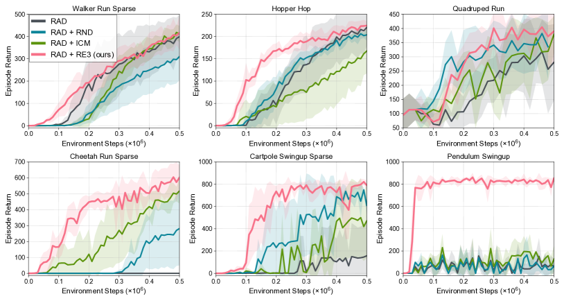
Comparison with other exploration methods. We also compare our state entropy maximization scheme to other exploration methods combined with RAD, i.e., RAD + RND and RAD + ICM, that learn additional models to obtain intrinsic rewards proportional to prediction errors. As shown in Figure 6, RAD + RE3 consistently exhibits superior sample efficiency in most tasks. While RND similarly employs a fixed random network for the intrinsic reward, it also introduces an additional network which requires training and therefore suffers from instability. This result demonstrates that RE3 can improve sample-efficiency without introducing additional models for exploration, by utilizing fixed representations from a random encoder for stable state entropy estimation.

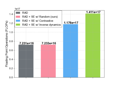
Compute-efficiency. We show that RE3 is a practical and scalable approach for exploration in RL due to its compute-efficiency. In particular, RE3 is compute-efficient in that (a) there are no gradient updates through the random encoder, and (b) there are no unnecessary forward passes for obtaining representations at every update step since we store low-dimensional latent representations in the replay buffer. To evaluate compute-efficiency, we show the floating point operations (FLOPs) consumed by RAD, RAD + SE w/ Random (ours), RAD + SE w/ Contrastive, and RAD + SE w/ Inverse dynamics. We account only for forward and backward passes through neural network layers. We explain our full procedure for counting FLOPs in Appendix F. Figure 7 shows the FLOPS used by each agent to achieve its final performance in Hopper Hop. One can see that estimating state entropy with a random encoder is significantly more compute-efficient than with a encoder learned by contrastive learning and inverse dynamics prediction. In particular, RAD + SE w/ Random requires 7.233e+16 FLOPs to achieve its performance at 500K steps, while RAD + SE w/ Inverse dynamics requires roughly twice as many. One important detail here is that RAD + SE w/ Random has comparable compute-efficiency to RAD. Therefore, we improve the sample-efficiency of RAD without sacrificing compute-efficiency.

Figure 7: Number of FLOPs used by each agent to achieve its performance at 500K environment steps in Hopper Hop (see Figure 5 for corresponding learning curves).

Figure 8: Observations from evenly-spaced intervals for one episode of executing policy actions. As a baseline, we show random exploration, i.e. sampling from the action space uniformly at random. We compare the diversity of visited states resulting from pre-training for 500K steps with APT (Liu & Abbeel, 2021) and RE3 (ours). We provide corresponding videos in our website.

(a) Ground-truth state entropy estimate

(b) Hopper Hop

(c) Hopper Stand

Figure 9: (a) We observe that pre-training Hopper agent with RE3 results in a higher state entropy estimate in the ground-truth state space, i.e., proprioceptive state space, compared to other state entropy maximization schemes that involve representation learning. This shows that maximizing state entropy in the fixed representation space of a randomly initialized encoder effectively encourages the agent to visit a wide range of states. We show that this leads to better sample-efficiency when fine-tuning pre-trained policies on (b) Hopper Hop and (c) Hopper Stand. The solid (or dotted) line and shaded regions represent the mean and standard deviation, respectively, across three runs.

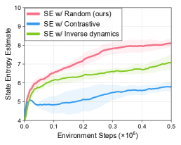
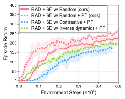
Evaluation of unsupervised pre-training. To evaluate the effectiveness of RE3 for learning diverse behaviors in the pre-training phase without extrinsic rewards, we visualize the behaviors of policies pre-trained for 500K environment steps in Figure 8. One can see that the pre-trained policy using RE3 exhibits more diverse behaviors compared to random exploration or APT (Liu & Abbeel, 2021), where a policy is pre-trained to maximize state entropy estimate in contrastive representation space. To further evaluate the diversity of behaviors quantitatively, we show the state entropy estimate in the ground-truth state space of Hopper environment in Figure 9(a), which is computed using distances between all proprioceptive states in the current minibatch. We observe that RE3 exhibits a higher ground-truth state entropy estimate than state entropy maximization schemes that use contrastive learning and inverse dynamics prediction during pre-training. This implies that RE3 can effectively maximize the ground-truth state entropy without being able to directly observe underlying ground-truth states.

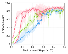
Fine-tuning in downstream tasks. We also remark that the diversity of behaviors leads to superior sample-efficiency when fine-tuning a pre-trained policy in downstream tasks, as shown in Figure 9(b) and 9(c). Specifically, we fine-tune a pre-trained policy in downstream tasks where extrinsic rewards are available, by initializing the parameters of policies with parameters of pre-trained policies (see Appendix A for more details). We found that fine-tuning a policy pre-trained with RE3 (RAD + SE w/ Random + PT) further improves the sample-efficiency of RAD + SE w/ Random, and also outperforms other pre-training schemes. We emphasize that RE3 allows learning such diverse behaviors by pre-training a policy only for 500K environment steps, while previous work (Liu & Abbeel, 2021) reported results by training for 5M environment steps.

(a) Robustness to noise by ensemble (b) Robustness to color changes by ensemble (c) Effects of 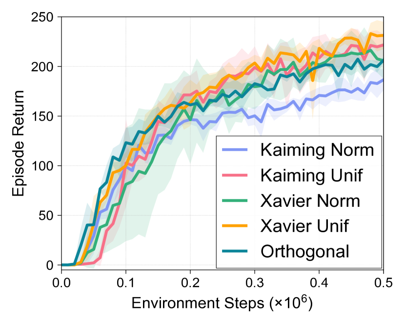$k$ (d) Effects of Initialization

Figure 10: We observe that introducing an ensemble of random encoders can improve robustness to (a) simple Gaussian noise and (b) color changes. Performance of RAD + RE3 with varying (c) $k$ and (d) the initialization of a random encoder on Hopper Hop environment.

Figure 11: Performance on navigation tasks from MiniGrid. A2C + RE3 outperforms other exploration methods in terms of sample-efficiency, and A2C + RE3 + PT further improves sample-efficiency. The solid (or dotted) line and shaded regions represent the mean and standard deviation, respectively, across five runs.

Robustness to noise and perturbations via ensembles. We consider a simple extension of our approach by introducing an ensemble of random encoders and found that this improves robustness to simple Gaussian noise see Figure 10(a). We also remark that random encoders can be useful not only for compute-efficiency, but also for $k$-NN selection in more diverse scenarios. For example, when the background color changes randomly, one might want to ignore the background color and select $k$-NNs with similar joint positions. In Figure 10(b), we demonstrate that $k$-NN in raw pixel space only finds observations with similar background colors, while the ensemble of random encoders can find observations with similar joint positions but different colors, as averaging features of convolutional encoders with different initializations could improve robustness to low-level features like colors and textures (Lee et al., 2020).

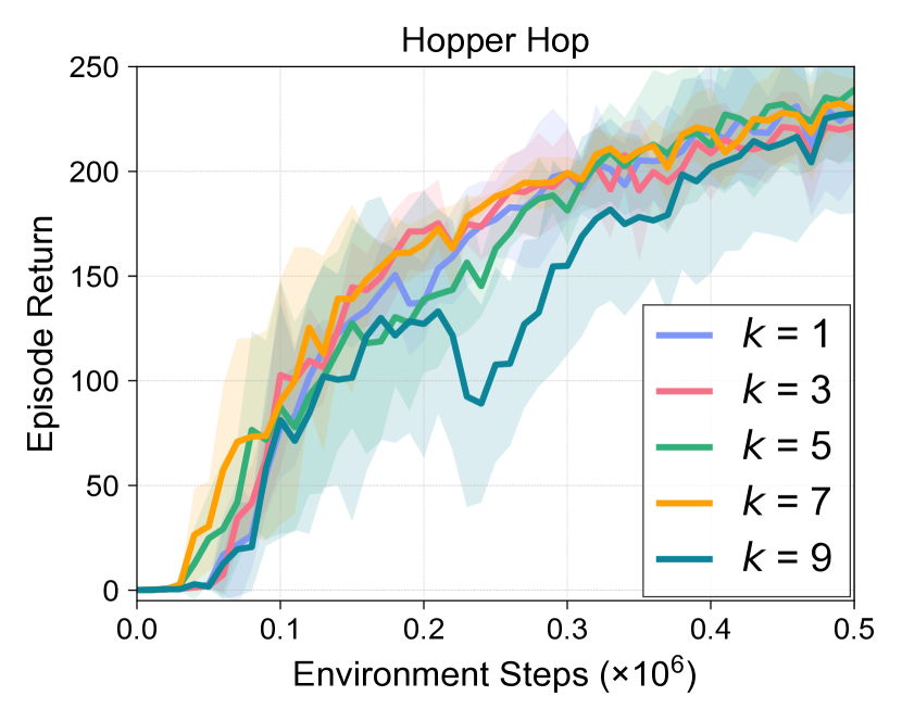
Sensitivity analysis to hyperparameters. We investigate how hyperparameters affect the performance of RE3. Specifically, we consider $k\in\{1,3,5,7,9\}$ for $k$-NN in (2), and various initialization schemes for a random encoder, i.e., the Xavier initialization (also called the Glorot initialization; Glorot & Bengio 2010), the He initialization (He et al., 2015), and the Orthogonal initialization (Saxe et al., 2014). Figure 10(c) and Figure 10(d) show that RE3 is robust to such considered hyperparameters.

4.2 MiniGrid Experiments

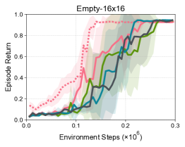
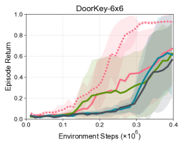
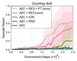
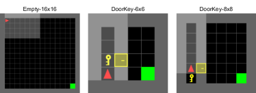
Setup. We evaluate our method on MiniGrid (Chevalier-Boisvert et al., 2018), a gridworld environment with a selection of sparse reward tasks. We consider the following setups where the agent obtains a reward only by reaching the green goal square: Empty, a large room with the goal in the furthest corner; DoorKey, where the agent must collect a key and unlock a door before entering the room containing the goal. The tasks are shown in Figure 12. For evaluation, we consider two exploration methods, RND and ICM. For our method and other exploration methods, we use Advantage Actor-Critic (A2C; Mnih et al. (2016)) as the underlying RL algorithm. In all tasks, the agent has access to a compact $7\times 7\times 3$ embedding of the $7\times 7$ grid directly in front of it, making the environment partially-observable. To combine RE3 with A2C, an on-policy RL method, we maintain a replay buffer of 10K samples solely for computing the RE3 intrinsic reward, and compute $k$-NN distances between the on-policy batch and the entire replay buffer. For RND and ICM, the intrinsic reward is computed using the on-policy batch. For RE3, ICM, and RND, we perform hyperparameter search over the intrinsic reward weight and report the best result (see the Appendix C for more details).

Figure 12: Navigation tasks from MiniGrid (Chevalier-Boisvert et al., 2018) used in our experiments. The agent is represented as a red arrow and the light gray region shows the $7\times 7$ (or smaller, if obstructed by walls) grid which the agent observes. The agent receives a positive reward only for reaching the green square.

(a) Montezuma’s Revenge

(b) Beam Rider

(c) Human Normalized Score

Figure 13: Performance on (a) Montezuma’s Revenge and (b) Beam Rider games. (c) Human normalized score averaged over six Atari games. The solid line and shaded regions represent the mean and standard deviation, respectively, across three runs.

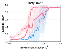
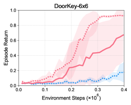
Comparison with other exploration methods. Figure 11 shows that RE3 is more effective for improving the sample-efficiency of A2C in most tasks, compared to other exploration methods, RND and ICM, that learn additional models. In particular, A2C + RE3 achieves average episode return of 0.49 at 2.4M environment steps in DoorKey-8x8; in comparison, A2C + ICM achieves a return of 0.20 and A2C + RND and A2C both fail to achieve non-trivial returns. These results demonstrate that state entropy maximization with RE3 can also improve the sample-efficiency of on-policy RL algorithms by introducing only a small-size replay buffer.

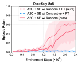
Fine-tuning in downstream tasks. To evaluate the effectiveness of RE3 for unsupervised pre-training in MiniGrid tasks, we first pre-train a policy in a large vacant room (Empty-16$\times$16) to maximize RE3 intrinsic rewards for 100K environment steps. Then, we fine-tune the pre-trained policy in downstream tasks by initializing a policy with pre-trained parameters and subsequently training with A2C + RE3. Figure 11 shows that A2C + RE3 + PT significantly improves the sample-efficiency of A2C, which demonstrates that the ability to explore novel states in a large empty room helps improve sample-efficiency in DoorKey tasks, which involve the added complexity of additional components, e.g., walls, doors, and locks. We show a comparison to state entropy maximization with contrastive learning in Figure 16 and observe that it does not work well, as contrastive learning depends on data augmentation specific to images (e.g., random shift and color jitter), which are not compatible with the compact embeddings used as inputs for MiniGrid. RE3 effectively eliminates the need for carefully chosen data augmentations by employing a random encoder.

4.3 Atari Experiments

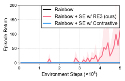
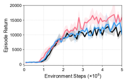
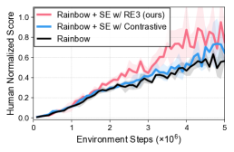
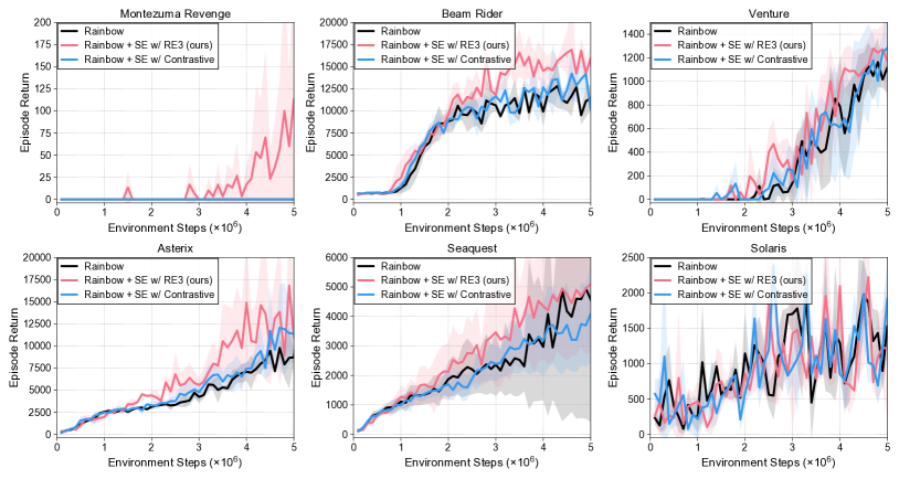
We also evaluate RE3 on Atari games from Arcade Learning Environment (Bellemare et al., 2013). We use Rainbow (Hessel et al., 2018) as the underlying RL algorithm, and use convolutional neural networks with the same architecture as in Rainbow for random encoders. For evaluation, we perform hyperparameter search over the intrinsic reward weight for each environment, and report the human normalized score (Mnih et al., 2015) over six Atari games (see Appendix D for more details). Figure 13 shows that RE3 exhibits superior sample-efficiency compared to Rainbow and Rainbow + SE w/ Contrastive on various Atari games, including hard exploration games like Montezuma’s revenge (see Figure 15 for additional experimental results). These results demonstrate that random encoders can also be useful in more visually complex environments.

5 Discussion

In this paper, we present RE3, a simple exploration method compatible with both model-free and model-based RL algorithms. RE3 maximizes a $k$-nearest neighbor state entropy estimate in the fixed representation space of a randomly initialized encoder, which effectively captures information about similarity between states without any training. Our experimental results demonstrate that RE3 can encourage exploration in widely-used benchmarks, as it enables stable and compute-efficient state entropy estimation. Here, we emphasize that our goal is not to claim that representation learning or additional models are not required for exploration, but to show that fixed random encoders can be useful for efficient exploration. For more visually complex domains, utilizing pre-trained fixed representations for stable state entropy estimation could be more useful, but we leave it to future work to explore this direction further because this would require having access to environments and a wide distribution of states for pre-training, which is itself a non-trivial problem. Another interesting direction would be to investigate the effect of network architectures for state entropy estimation, or to utilize state entropy for explicitly guiding the action of a policy to visit diverse states. We believe RE3 would facilitate future research by providing a simple-to-implement, stable, and compute-efficient module that can be easily combined with other techniques.

Appendix

Appendix A Details on DeepMind Control Suite Experiments

A.1 Environments

We evaluate the performance of RE3 on various tasks from DeepMind Control Suite (Tassa et al., 2020). For Hopper Hop, Quadruped Run, Cartpole Swingup Sparse, Pendulum Swingup, we use the publicly available environments without any modification. For environments which are not from the publicly available released implementation repository (https://github.com/deepmind/dm_control), we designed the tasks following Seyde et al. (2021) as below:

• Walker/Cheetah Run Sparse: The goal of Walker/Cheetah Run Sparse task is same as in Walker/Cheetah Run, moving forward as fast as possible, but reward is given sparsely until it reaches a certain threshold: $r=r_{\tt{original}}\cdot\mathds{1}_{r_{\tt{original}}>0.25}$, where $r_{\tt{original}}$ is the reward in Walker/Cheetah Run from DeepMind Control Suite.

A.2 Implementation Details for Model-free RL

For all experimental results in this work, we report the results obtained by running experiments using the publicly available released implementations from the authors, i.e., RAD (https://github.com/MishaLaskin/rad) and DrQ (https://github.com/denisyarats/drq). We use random crop augmentation for RAD and random shift augmentation for DrQ. We provide a full list of hyperparameters in Table 1.

Implementation details for RE3. We highlight key implementation details for RE3:

• Intrinsic reward. We use $r^{\tt{i}}(s_{i}):=||y_{i}-y^{\text{$k$-NN}}_{i}||_{2}$ for the intrinsic reward. We got rid of $\log$ from intrinsic reward in (3) for simplicity in DeepMind Control Suite experiments, but results using $\log$ are also similar. To make the scale of intrinsic reward $r^{\tt{i}}$ consistent across tasks, following Liu & Abbeel (2021), we normalize the intrinsic reward by dividing it by a running estimate of the standard deviation. As for newly introduced hyperparameters, we use $k=3$, and perform hyperparameter search over $\beta_{0}\in\{0.05,0.25\}$ and $\rho\in\{0.00001,0.000025\}$.

• Architecture. For all model-free RL methods, we use the same encoder architecture as in Yarats et al. (2021). Specifically, this encoder consists of 4 convolutional layers followed by ReLU activations. We employ kernels of size 3 $\times$ 3 with 32 channels for all layers, and 1 stride except of the first layer which has stride 2. The output of convolutional layers is fed into a single fully-connected layer normalized by LayerNorm (Ba et al., 2016). Finally, tanh nonlinearity is added to the 50-dimensional output of the fully-connected layer.

• Unsupervised pre-training. For unsupervised pre-training, we first train a policy to maximize intrinsic rewards in (3) without extrinsic rewards for 500K environment steps. For fine-tuning a policy in downstream tasks, we initialize the parameters using the pre-trained parameters and then learn a policy to maximize RE3 objective in (4) for 500K environment steps. To stabilize the initial fine-tuning phase by making the scale of intrinsic reward consistent across pre-training and fine-tuning, we load the running estimate of the standard deviation from pre-training phase.

Implementation details for representation learning baselines . We highlight key implementation details for state entropy maximization schemes that involve representation learning, i.e., contrastive learning and inverse dynamics prediction, and that employs a pre-trained ImageNet Encoder:

• Contrastive learning. For state entropy maximization with contrastive learning, we introduce a separate convolutional encoder with randomly initialized parameters learned to minimize contrastive loss (Srinivas et al., 2020). Note that we use the separate encoder to investigate the independent effect of representation learning. Then we compute intrinsic reward $r^{\tt{i}}$ using representations obtained by processing observations through this separate encoder.

• Inverse dynamics prediction. For state entropy maximization with inverse dynamics prediction, we introduce a separate convolutional encoder with randomly initialized parameters learned to predict actions from two consecutive observations. Specifically, we introduce 2 fully-connected layers with ReLU activations to predict actions on top of encoder representations. We remark that this separate encoder is separate from RL. Then we compute intrinsic reward $r^{\tt{i}}$ using representations obtained by processing observations through this separate encoder.

• Pre-trained ImageNet encoder. For state entropy maximization with pre-trained ImageNet encoder, we utilize a ResNet-50 (He et al., 2016) encoder from publicly available torchvision models (https://pytorch.org/vision/0.8/models.html). To compute intrinsic reward $r^{\tt{i}}$, we utilize representations obtained by processing observations through this pre-trained encoder.

• Pre-trained ATC encoder. For state entropy maximization with pre-trained ATC (Stooke et al., 2021) encoder, we utilize pre-trained encoders from the authors. Specifically, these encoders are pre-trained by contrastive learning on pre-training datasets that contain samples encountered while training a RAD agent on DeepMind Control Suite environments (see Stooke et al. (2021) for more details). We use pre-trained parameters from Walker Run, Hopper Stand, and Cheetah Run for RAD + SE w/ ATC on Walker Run Sparse, Hopper Hop, and Cheetah Run Sparse, respectively. To compute intrinsic reward $r^{\tt{i}}$, we utilize representations obtained by processing observations through this pre-trained encoder.

Implementation details for exploration baselines. We highlight key implementation details for exploration baselines, i.e., RND (Burda et al., 2019) and ICM (Pathak et al., 2017):

• RND. For RND, we introduce a random encoder $f_{\theta}$ whose architecture is same as in Yarats et al. (2021), and introduce a predictor network $g_{\phi}$ consisting of a convolutional encoder with the same architecture and 2-layer fully connected network with 1024 units each. Then, parameters $\phi$ of the predictor network are trained to predict representations from a random encoder given the same observations, i.e., minimize $\epsilon=||f_{\theta}(s_{i})-g_{\phi}(s_{i})||_{2}$. We use prediction error $\epsilon$ as an intrinsic reward and learn a policy that maximizes $r^{\tt{total}}=r^{\tt{e}}+\beta\cdot r^{\tt{i}}$. We perform hyperparameter search over the weight $\beta\in\{0.05,0.1,1.0,10.0\}$ and report the best result on each environment.

• ICM. For ICM, we introduce a convolutional encoder $g_{\phi}$ whose architecture is same as in Yarats et al. (2021), and introduce a inverse dynamics predictor $h_{\psi}$ with 2 fully-connected layers with 1024 units. These networks are learned to predict actions between two consecutive observations, i.e., minimize $\mathcal{L}_{\tt{inv}}=||a_{t}-h_{\psi}(g_{\phi}(s_{t}),g_{\phi}(s_{t+1}))||_{2}$. We also introduce a forward dynamics predictor $f_{\Psi}$ that is learned to predict the representation of next time step, i.e., minimize $\mathcal{L}_{\tt{forward}}=\frac{1}{2}||g_{\phi}(s_{t+1})-f_{\Psi}(g_{\phi}(s_{t}),a_{t})||^{2}_{2}$. Then, we use prediction error as an intrinsic reward and learn a policy that maximizes $r^{\tt{total}}=r^{\tt{e}}+\beta\cdot r^{\tt{i}}$. For joint training of the forward and inverse dynamics, following Pathak et al. (2017), we minimize $0.2\cdot\mathcal{L}_{\tt{forward}}+0.8\cdot\mathcal{L}_{\tt{inv}}$. We perform hyperparameter search over the weight $\beta\in\{0.05,0.1,1.0\}$ and report the best result on each environment.

A.3 Implementation Details for Model-based RL.

For Dreamer, we use the publicly available released implementation repository (https://github.com/danijar/dreamer) from the authors. We highlight key implementation details for the combination of Dreamer with RE3:

• Intrinsic reward. We use $r^{\tt{i}}(s_{i}):=||y_{i}-y^{\text{$k$-NN}}_{i}||_{2}$ for the intrinsic reward. We got rid of $\log$ from intrinsic reward in (3) for simplicity in DeepMind Control Suite experiments, but results using $\log$ are also similar. To make the scale of intrinsic reward $r^{\tt{i}}$ consistent across tasks, following Liu & Abbeel (2021), we normalize the intrinsic reward by dividing it by a running estimate of the standard deviation. Since Dreamer utilizes trajectory segments for training batch, we use large value of $k=50$ to avoid find $k$-NN only within a trajectory segment. We also use $\beta_{0}=0.1$, and $\rho=0.0$, i.e., no decay schedule. We also remark that we find $k$-NN only within a minibatch instead of the entire buffer as in model-free RL, since the large batch size of Dreamer is enough for stable entropy estimation.

• Architecture. We use the same convolutional architecture as in Dreamer. Specifically, this encoder consists of 4 convolutional layers followed by ReLU activations. We employ kernels of size 4 $\times$ 4 with $\{32,64,128,256\}$ channels, and 2 stride for all layers. To obtain low-dimensional representations, we additionally introduce a fully-connected layer normalized by LayerNorm (Ba et al., 2016). Finally, tanh nonlinearity is added to the 50-dimensional output of the fully-connected layer.

Table 1: Hyperparameters of RAD + RE3 used for DeepMind Control Suite experiments.

Hyperparameter	Value
Augmentation	Crop
Observation rendering	$(100,100)$
Observation downsampling	$(84,84)$
Replay buffer size	$100000$
Initial steps	$10000$ quadruped, run; $1000$ otherwise
Stacked frames	$3$
Action repeat	$4$ quadruped, run; $2$ otherwise
Learning rate (actor, critic)	$0.0002$
Learning rate ($\alpha$)	$0.001$
Batch size	$512$
$Q$ function EMA $\tau$	$0.01$
Encoder EMA $\tau$	$0.05$
Critic target update freq	$2$
Convolutional layers	$4$
Number of filters	$32$
Latent dimension	$50$
Initial temperature	$0.1$ RAD + RE3; $0.01$ RAD + RE3 + PT
$k$	3
Initial intrinsic reward scale $\beta_{0}$	$0.25$ pendulum, swingup; $0.05$ otherwise
Intrinsic reward decay $\rho$	$0.000025$ walker, run sparse; $0.00001$ otherwise
Intrinsic reward scale (RND)	$10.0$ cartpole, swingup sparse
	$0.1$ pendulum, swingup; cheetah, run sparse
	$0.05$ otherwise
Intrinsic reward scale (ICM)	$1.0$ cheetah, run sparse
	$0.1$ otherwise

Table 2: Hyperparameters of Dreamer + RE3 used for DeepMind Control Suite experiments. We only specify hyperparameters different from original paper of Hafner et al. (2020).

Hyperparameter	Value
Initial episodes	$5$
Precision	$32$
Latent dimension of a random encoder	50
$k$	53
Initial reward scale $\beta_{0}$	0.1
Intrinsic reward decay $\rho$	$0.0$

Appendix B Additional Experimental Results on DeepMind Control Suite

We provide additional experimental results on various tasks from DeepMind Control Suite (Tassa et al., 2020). We observe that RE3 improves sample-efficiency in several tasks, e.g., Reacher Hard and Hopper Stand, while not degrading the performance in dense-reward tasks like Cartpole Balance. This demonstrates the simple and wide applicability of RE3 to various tasks.

Figure 14: Performance on locomotion tasks from DeepMind Control Suite. The solid line and shaded regions represent the mean and standard deviation, respectively, across five runs.

Appendix C Details on MiniGrid Experiments

For our A2C implementation in MiniGrid, we use the publicly available released implementation repository (https://github.com/lcswillems/rl-starter-files) and use their default hyperparameters. We provide a full list of hyperparameters that are introduced by our method or emphasized for clarity in Table 3.

We highlight some key implementation details:

• We use $r^{\tt{i}}(s_{i}):=\log(||y_{i}-y^{\text{$k$-NN}}_{i}||_{2}+1)$ for the intrinsic reward. The additional $1$ is for numerical stability.

• We use the average distance between $y_{i}$ and its $k$ nearest neighbors (i.e., $y^{\text{$2$-NN}}_{i},\cdots,y^{\text{$k$-NN}}_{i}$) for the intrinsic reward, instead of the single $k$ nearest neighbor. This provides a less noisy state entropy estimate and empirically improves performance in MiniGrid environments.

• We perform hyperparameter search over $\beta\in\{0.00001,0.00005,0.0001,0.0005,0.001,0.005,\\ 0.01,0.05,0.1\}$ for RE3, ICM, and RND and report the best result.

• We do not change the network architecture from the above publicly available implementation. We use the same encoder architecture as the RL encoder for state entropy maximization. This encoder architecture consists of 3 convolutional layers with kernel 2, stride 1, and padding 0, each followed by a ReLU layer. The convolutional layers have 16, 32, and 64 filters respectively. The first ReLU is followed by a two-dimensional max pooling layer with kernel 2. The actor and critic MLPs both contain two fully-connected layers with hidden dimension 64, with a tanh operation in between.

Table 3: Hyperparameters used for MiniGrid experiments. Most hyperparameter values are unchanged across environments with the exception of evaluation frequency and intrinsic reward weight $\beta$.

Hyperparameter	Value
Input Size	$(7,7,3)$
Replay buffer size (for RE3 intrinsic reward)	10000
Stacked frames	$1$
Action repeat	$1$
Evaluation episodes	$100$
Optimizer	RMSprop
$k$	3
Evaluation frequency	$6400$ Empty-16x16; $12800$ DoorKey-6x6
	$64000$ DoorKey-8x8
Intrinsic reward weight $\beta$ in Empty-16x16 experiments	$0.1$ A2C + RE3 + PT
	$0.1$ A2C + RE3
	$0.00001$ A2C + ICM
	$0.00005$ A2C + RND
Intrinsic reward weight $\beta$ in DoorKey-6x6 experiments	$0.05$ A2C + RE3 + PT
	$0.005$ A2C + RE3
	$0.0001$ A2C + ICM
	$0.0001$ A2C + RND
Intrinsic reward weight $\beta$ in DoorKey-8x8 experiments	$0.05$ A2C + RE3 + PT
	$0.01$ A2C + RE3
	$0.001$ A2C + ICM
	$0.00005$ A2C + RND
Intrinsic reward decay $\rho$	$0$
Number of processes	$16$
Frames per process	$5$
Discount $\gamma$	0.99
GAE $\lambda$	0.95
Entropy coefficient	$0.01$
Value loss term coefficient	$0.5$
Maximum norm of gradient	$0.5$
RMSprop $\epsilon$	$0.01$
Clipping $\epsilon$	$0.2$
Recurrence	None

Appendix D Details on Atari Experiments

For our Rainbow implementation in Atari games, we use the publicly available implementation repository (https://github.com/Kaixhin/Rainbow) and use their default hyperparameters.

We highlight some key implementation details:

• We use $r^{\tt{i}}(s_{i}):=\log(||y_{i}-y^{\text{$k$-NN}}_{i}||_{2}+1)$ for the intrinsic reward. The additional $1$ is for numerical stability.

• We perform hyperparameter search over $\beta\in\{0.0001,0.001,0.01\}$ for Rainbow + SE w/ RE3 and report the best result for each environment. We used $0.01$ for Asterix and BeamRider, $0.001$ for Seaquest, and $0.0001$ for other games.

• We perform hyperparameter search over $\beta\in\{0.0001,0.001\}$ for Rainbow + SE w/ Contrastive and report the best result for each environment. Specifically, we used $0.001$ for Seaquest, $0.0001$ for other games.

• We do not change the network architecture from the above publicly available implementation. We use the same encoder architecture as the RL encoder for state entropy maximization, with additional linear layer to reduce the dimension of latent representations. This encoder consists of 3 convolutional layers with kernels $\{8,4,3\}$, strides $\{4,4,3\}$, and padding 0, each followed by a ReLU layer. The convolutional layers have 32, 32, 64 filters, respectively. Then the outputs from a convolutional encoder is flattened and followed by a linear layer of size $\{50,150\}$. We find that large dimension of 150 is effective for Montezuma’s Revenge, but 50 is enough for all other environments.

Appendix E Additional Experimental Results on Atari Games

Figure 15: Performance on Atari games from Arcade Learning Environment. The solid line and shaded regions represent the mean and standard deviation, respectively, across three runs.

Appendix F Calculation of Floating Point Operations

We explain our FLOP counting procedure for comparing the compute-efficiency of RAD, RAD + SE w/ Random (ours), RAD + SE w/ Contrastive, and RAD + SE w/ Inverse dynamics in Figure 7. We consider each backward pass to require twice as many FLOPs as a forward pass, as done in https://openai.com/blog/ai-and-compute/. Each weight requires one multiply-add operation in the forward pass. In the backward pass, it requires two multiply-add operations: at layer $i$, the gradient of the loss with respect to the weight at layer $i$ and with respect to the output of layer ($i-1$) need to be computed. The latter computation is necessary for subsequent gradient calculations for weights at layer ($i-1$).

We use functions from Huang et al. (2018) and Jeong & Shin (2019) to obtain the number of operations per forward pass for all layers in the encoder (denoted $E$) and number of operations per forward pass for all MLP layers (denoted $M$).

We assume that (1) the number of updates per iteration is 1, (2) the architecture of the encoder used for state entropy estimation is the same as the RL encoder used in RAD, and (3) the FLOPs required for computations (e.g., finding the $k$-NNs in representation space) that are not forward and backward passes through neural network layers is negligible.

We denote the number of forward passes per training update $F$, the number of backward passes per training update $B$, and the batch size $b$ (in our experiments $b=512$). Then, the number of FLOPs per iteration of RAD is:

$bF(E+M)+2bB(E+M)+(E+M),$

where the last term is for the single forward pass required to compute the policy action.

Specifically, RAD + SE w/ Random only requires $E$ extra FLOPs per iteration to store the fixed representation from the random encoder in the replay buffer for future $k$-NN calculations. In comparison, RAD + SE w/ Contrastive requires $4bE$ extra FLOPs per iteration, and RAD + SE w/ Inverse dynamics requires more than $6bE$ extra FLOPs.

Appendix G Comparison to State Entropy Maximization with Contrastive Encoder for MiniGrid Pre-training

We show a comparison to state entropy maximization with contrastive learning (i.e., A2C + SE w/ Contrastive + PT) in Figure 16. In the results shown, we do not use state entropy intrinsic reward during the fine-tuning phase for A2C + SE w/ Contrastive + PT, following the setup of Liu & Abbeel (2021), but found that using intrinsic reward during fine-tuning results in very similar performance. As discussed in Section 4.2, we observe that the contrastive encoder does not work well for state entropy estimation, as contrastive learning depends on data augmentation specific to images (e.g., random shift, random crop, and color jitter), which are not compatible with the compact embeddings used as inputs for MiniGrid. We re-mark that RE3 eliminates the need for carefully chosen data augmentations by employing a random encoder.

Figure 16: Performance on navigation tasks from MiniGrid. We find that pre-training using state entropy (SE) with a random encoder (ours) outperforms pre-training using state entropy with a contrastive encoder (Liu & Abbeel, 2021), using random shift as the data augmentation. The solid (or dotted) line and shaded regions represent the mean and standard deviation, respectively, across five runs.

Appendix H RE3 with On-policy Reinforcement Learning

We provide the full procedure for RE3 with on-policy RL in Algorithm 2.

Algorithm 2 RE3: On-policy RL version

1:  Initialize parameters of random encoder $\theta$, policy $\phi$

2:  Initialize replay buffer $\mathcal{B}\leftarrow\emptyset$, step counter $t\leftarrow 0$

3:  repeat

4:     // Collect transitions

5:     $t_{\tt{start}}\leftarrow t$

6:     repeat

7:        Collect a transition $\tau_{t}=(s_{t},a_{t},s_{t+1},r^{\tt{e}}_{t})$ from the interaction with the environment using policy $\pi_{\phi}$

8:        Get a fixed representation $y_{t}=f_{\theta}(s_{t})$

9:        $\mathcal{B}\leftarrow\mathcal{B}\cup\{(\tau_{t},y_{t})\}$

10:        $t\leftarrow t+1$

11:     until terminal $s_{t}$ or $t-t_{\tt{start}}=t_{\tt{max}}$

12:     // Compute intrinsic reward

13:     for $j=t-1$ to $t_{\tt{start}}$ do

14:        Compute the distance $||y_{j}-y||_{2}$ for all representations $y\in\mathcal{B}$ and find the $k$-nearest neighbor $y_{j}^{\text{$k$-NN}}$

15:        Compute $r_{j}^{\tt{i}}\leftarrow\log(||y_{j}-y_{j}^{\text{$k$-NN}}||_{2}+1)$

16:        Let $r^{\tt{total}}_{j}\leftarrow r_{j}^{\tt{e}}+\beta\cdot r_{j}^{\tt{i}}$

17:     end for

18:     // Update policy

19:     Update $\phi$ with transitions $\{(s_{j},a_{j},s_{j+1},r_{j}^{\tt{total}})\}_{j=t_{\tt{start}}}^{t-1}$

20:  until $t>t_{\tt{max}}$

References

- Ba et al. (2016) Ba, J. L., Kiros, J. R., and Hinton, G. E. Layer normalization. arXiv preprint arXiv:1607.06450, 2016.
- Badia et al. (2020) Badia, A. P., Sprechmann, P., Vitvitskyi, A., Guo, D., Piot, B., Kapturowski, S., Tieleman, O., Arjovsky, M., Pritzel, A., Bolt, A., et al. Never give up: Learning directed exploration strategies. In International Conference on Learning Representations, 2020.
- Beirlant et al. (1997) Beirlant, J., Dudewicz, E. J., Györfi, L., and Van der Meulen, E. C. Nonparametric entropy estimation: An overview. International Journal of Mathematical and Statistical Sciences, 6(1):17–39, 1997.
- Bellemare et al. (2016) Bellemare, M., Srinivasan, S., Ostrovski, G., Schaul, T., Saxton, D., and Munos, R. Unifying count-based exploration and intrinsic motivation. In Advances in Neural Information Processing Systems, 2016.
- Bellemare et al. (2013) Bellemare, M. G., Naddaf, Y., Veness, J., and Bowling, M. The arcade learning environment: An evaluation platform for general agents. Journal of Artificial Intelligence Research, 47:253–279, 2013.
- Burda et al. (2019) Burda, Y., Edwards, H., Storkey, A., and Klimov, O. Exploration by random network distillation. In International Conference on Learning Representations, 2019.
- Caron et al. (2018) Caron, M., Bojanowski, P., Joulin, A., and Douze, M. Deep clustering for unsupervised learning of visual features. In Proceedings of the European Conference on Computer Vision, 2018.
- Chevalier-Boisvert et al. (2018) Chevalier-Boisvert, M., Willems, L., and Pal, S. Minimalistic gridworld environment for openai gym. https://github.com/maximecb/gym-minigrid, 2018.
- Colas et al. (2019) Colas, C., Fournier, P., Chetouani, M., Sigaud, O., and Oudeyer, P.-Y. Curious: intrinsically motivated modular multi-goal reinforcement learning. In International Conference on Machine Learning, 2019.
- Florensa et al. (2018) Florensa, C., Held, D., Geng, X., and Abbeel, P. Automatic goal generation for reinforcement learning agents. In International Conference on Machine Learning, 2018.
- Fortunato et al. (2018) Fortunato, M., Azar, M. G., Piot, B., Menick, J., Osband, I., Graves, A., Mnih, V., Munos, R., Hassabis, D., Pietquin, O., et al. Noisy networks for exploration. In International Conference on Learning Representations, 2018.
- Gaier & Ha (2019) Gaier, A. and Ha, D. Weight agnostic neural networks. In Advances in Neural Information Processing Systems, 2019.
- Gamba et al. (1961) Gamba, A., Gamberini, L., Palmieri, G., and Sanna, R. Further experiments with papa. Il Nuovo Cimento (1955-1965), 20(2):112–115, 1961.
- Glorot & Bengio (2010) Glorot, X. and Bengio, Y. Understanding the difficulty of training deep feedforward neural networks. In International Conference on Artificial Intelligence and Statistics, 2010.
- Haarnoja et al. (2018) Haarnoja, T., Zhou, A., Abbeel, P., and Levine, S. Soft actor-critic: Off-policy maximum entropy deep reinforcement learning with a stochastic actor. In International Conference on Machine Learning, 2018.
- Hafner et al. (2020) Hafner, D., Lillicrap, T., Ba, J., and Norouzi, M. Dream to control: Learning behaviors by latent imagination. In International Conference on Learning Representations, 2020.
- Hazan et al. (2019) Hazan, E., Kakade, S., Singh, K., and Van Soest, A. Provably efficient maximum entropy exploration. In International Conference on Machine Learning, 2019.
- He et al. (2015) He, K., Zhang, X., Ren, S., and Sun, J. Delving deep into rectifiers: Surpassing human-level performance on imagenet classification. In Proceedings of the IEEE international conference on computer vision, 2015.
- He et al. (2016) He, K., Zhang, X., Ren, S., and Sun, J. Deep residual learning for image recognition. In Proceedings of the IEEE conference on computer vision and pattern recognition, 2016.
- Hessel et al. (2018) Hessel, M., Modayil, J., Van Hasselt, H., Schaul, T., Ostrovski, G., Dabney, W., Horgan, D., Piot, B., Azar, M., and Silver, D. Rainbow: Combining improvements in deep reinforcement learning. In Proceedings of the AAAI Conference on Artificial Intelligence, 2018.
- Houthooft et al. (2016) Houthooft, R., Chen, X., Duan, Y., Schulman, J., De Turck, F., and Abbeel, P. Vime: Variational information maximizing exploration. In Advances in Neural Information Processing Systems, 2016.
- Huang et al. (2018) Huang, G., Liu, S., Van der Maaten, L., and Weinberger, K. Q. Condensenet: An efficient densenet using learned group convolutions. In IEEE conference on computer vision and pattern recognition, 2018.
- Jeong & Shin (2019) Jeong, J. and Shin, J. Training cnns with selective allocation of channels. In International Conference on Machine Learning, 2019.
- Kaelbling et al. (1998) Kaelbling, L. P., Littman, M. L., and Cassandra, A. R. Planning and acting in partially observable stochastic domains. Artificial intelligence, 101(1-2):99–134, 1998.
- Kostrikov et al. (2021) Kostrikov, I., Yarats, D., and Fergus, R. Image augmentation is all you need: Regularizing deep reinforcement learning from pixels. In International Conference on Learning Representations, 2021.
- Laskin et al. (2020) Laskin, M., Lee, K., Stooke, A., Pinto, L., Abbeel, P., and Srinivas, A. Reinforcement learning with augmented data. In Advances in Neural Information Processing Systems, 2020.
- Lee et al. (2020) Lee, K., Lee, K., Shin, J., and Lee, H. Network randomization: A simple technique for generalization in deep reinforcement learning. In International Conference on Learning Representations, 2020.
- Lee et al. (2019) Lee, L., Eysenbach, B., Parisotto, E., Xing, E., Levine, S., and Salakhutdinov, R. Efficient exploration via state marginal matching. arXiv preprint arXiv:1906.05274, 2019.
- Lillicrap et al. (2016) Lillicrap, T. P., Hunt, J. J., Pritzel, A., Heess, N., Erez, T., Tassa, Y., Silver, D., and Wierstra, D. Continuous control with deep reinforcement learning. In International Conference on Learning Representations, 2016.
- Liu & Abbeel (2021) Liu, H. and Abbeel, P. Behavior from the void: Unsupervised active pre-training. In International Conference on Machine Learning, 2021.
- Minsky & Papert (1969) Minsky, M. and Papert, S. A. Perceptrons: An introduction to computational geometry. MIT press, 1969.
- Mnih et al. (2015) Mnih, V., Kavukcuoglu, K., Silver, D., Rusu, A. A., Veness, J., Bellemare, M. G., Graves, A., Riedmiller, M., Fidjeland, A. K., Ostrovski, G., et al. Human-level control through deep reinforcement learning. nature, 518(7540):529–533, 2015.
- Mnih et al. (2016) Mnih, V., Badia, A. P., Mirza, M., Graves, A., Lillicrap, T., Harley, T., Silver, D., and Kavukcuoglu, K. Asynchronous methods for deep reinforcement learning. In International Conference on Machine Learning, 2016.
- Mutti et al. (2021) Mutti, M., Pratissoli, L., and Restelli, M. A policy gradient method for task-agnostic exploration. In Proceedings of the AAAI Conference on Artificial Intelligence, 2021.
- Nair et al. (2018) Nair, A., Pong, V., Dalal, M., Bahl, S., Lin, S., and Levine, S. Visual reinforcement learning with imagined goals. In Advances in Neural Information Processing Systems, 2018.
- Ostrovski et al. (2017) Ostrovski, G., Bellemare, M. G., Oord, A. v. d., and Munos, R. Count-based exploration with neural density models. In International Conference on Machine Learning, 2017.
- Pathak et al. (2017) Pathak, D., Agrawal, P., Efros, A. A., and Darrell, T. Curiosity-driven exploration by self-supervised prediction. In International Conference on Machine Learning, 2017.
- Pathak et al. (2019) Pathak, D., Gandhi, D., and Gupta, A. Self-supervised exploration via disagreement. In International Conference on Machine Learning, 2019.
- Plappert et al. (2018) Plappert, M., Houthooft, R., Dhariwal, P., Sidor, S., Chen, R. Y., Chen, X., Asfour, T., Abbeel, P., and Andrychowicz, M. Parameter space noise for exploration. In International Conference on Learning Representations, 2018.
- Pong et al. (2020) Pong, V. H., Dalal, M., Lin, S., Nair, A., Bahl, S., and Levine, S. Skew-fit: State-covering self-supervised reinforcement learning. In International Conference on Machine Learning, 2020.
- Rahimi & Recht (2007) Rahimi, A. and Recht, B. Random features for large-scale kernel machines. In Advances in Neural Information Processing Systems, 2007.
- Saxe et al. (2011) Saxe, A. M., Koh, P. W., Chen, Z., Bhand, M., Suresh, B., and Ng, A. Y. On random weights and unsupervised feature learning. In International Conference on Machine Learning, 2011.
- Saxe et al. (2014) Saxe, A. M., McClelland, J. L., and Ganguli, S. Exact solutions to the nonlinear dynamics of learning in deep linear neural networks. In International Conference on Learning Representations, 2014.
- Sekar et al. (2020) Sekar, R., Rybkin, O., Daniilidis, K., Abbeel, P., Hafner, D., and Pathak, D. Planning to explore via self-supervised world models. In International Conference on Machine Learning, 2020.
- Seyde et al. (2021) Seyde, T., Schwarting, W., Karaman, S., and Rus, D. Learning to plan optimistically: Uncertainty-guided deep exploration via latent model ensembles, 2021. URL https://openreview.net/forum?id=vT0NSQlTA.
- Singh et al. (2003) Singh, H., Misra, N., Hnizdo, V., Fedorowicz, A., and Demchuk, E. Nearest neighbor estimates of entropy. American journal of mathematical and management sciences, 23(3-4):301–321, 2003.
- Srinivas et al. (2020) Srinivas, A., Laskin, M., and Abbeel, P. Curl: Contrastive unsupervised representations for reinforcement learning. In Internatial Conference on Machine Learning, 2020.
- Stadie et al. (2015) Stadie, B. C., Levine, S., and Abbeel, P. Incentivizing exploration in reinforcement learning with deep predictive models. arXiv preprint arXiv:1507.00814, 2015.
- Stooke et al. (2021) Stooke, A., Lee, K., Abbeel, P., and Laskin, M. Decoupling representation learning from reinforcement learning. In International Conference on Machine Learning, 2021.
- Sutton & Barto (2018) Sutton, R. S. and Barto, A. G. Reinforcement learning: An introduction. MIT Press, 2018.
- Taïga et al. (2020) Taïga, A. A., Fedus, W., Machado, M. C., Courville, A., and Bellemare, M. G. Benchmarking bonus-based exploration methods on the arcade learning environment. In International Conference on Learning Representations, 2020.
- Tang et al. (2017) Tang, H., Houthooft, R., Foote, D., Stooke, A., Chen, O. X., Duan, Y., Schulman, J., DeTurck, F., and Abbeel, P. # exploration: A study of count-based exploration for deep reinforcement learning. In Advances in Neural Information Processing Systems, 2017.
- Tao et al. (2020) Tao, R. Y., François-Lavet, V., and Pineau, J. Novelty search in representational space for sample efficient exploration. In Advances in Neural Information Processing Systems, 2020.
- Tassa et al. (2020) Tassa, Y., Tunyasuvunakool, S., Muldal, A., Doron, Y., Liu, S., Bohez, S., Merel, J., Erez, T., Lillicrap, T., and Heess, N. dm_control: Software and tasks for continuous control. arXiv preprint arXiv:2006.12983, 2020.
- Ulyanov et al. (2018) Ulyanov, D., Vedaldi, A., and Lempitsky, V. Deep image prior. In Proceedings of the IEEE Conference on Computer Vision and Pattern Recognition, 2018.
- Vempala (2005) Vempala, S. S. The random projection method, volume 65. American Mathematical Soc., 2005.
- Wieting & Kiela (2019) Wieting, J. and Kiela, D. No training required: Exploring random encoders for sentence classification. In International Conference on Learning Representations, 2019.
- Yarats et al. (2021) Yarats, D., Zhang, A., Kostrikov, I., Amos, B., Pineau, J., and Fergus, R. Improving sample efficiency in model-free reinforcement learning from images. In Proceedings of the AAAI Conference on Artificial Intelligence, 2021.
- Ziebart (2010) Ziebart, B. D. Modeling purposeful adaptive behavior with the principle of maximum causal entropy, 2010.