Signal Propagation in a
Gradient-Based and Evolutionary Learning System

Abstract.

Generative adversarial networks (GANs) exhibit training pathologies that can lead to convergence-related degenerative behaviors, whereas spatially-distributed, coevolutionary algorithms (CEAs) for GAN training, e.g. Lipizzaner, are empirically robust to them. The robustness arises from diversity that occurs by training populations of generators and discriminators in each cell of a toroidal grid. Communication, where signals in the form of parameters of the best GAN in a cell propagate in four directions: North, South, West and East, also plays a role, by communicating adaptations that are both new and fit. We propose Lipi-Ring, a distributed CEA like Lipizzaner, except that it uses a different spatial topology, i.e. a ring. Our central question is whether the different directionality of signal propagation (effectively migration to one or more neighbors on each side of a cell) meets or exceeds the performance quality and training efficiency of Lipizzaner Experimental analysis on different datasets (i.e, MNIST, CelebA, and COVID-19 chest X-ray images) shows that there are no significant differences between the performances of the trained generative models by both methods. However, Lipi-Ring significantly reduces the computational time (14.2%$\dots$41.2%). Thus, Lipi-Ring offers an alternative to Lipizzaner when the computational cost of training matters.

1. Introduction

Generative modeling aims to learn a function that describes a latent distribution of a dataset. In a popular paradigm, a generative adversarial network (GAN) combines two deep neural networks (DNN), a generator and a discriminator, that engage in adversarial learning to optimize their weights (Goodfellow et al., 2014). The generator is trained to produce fake samples (given an input from a random space) to fool the discriminator. The discriminator learns to discern the real samples from the ones produced by the generator. This training is formulated as a minmax optimization problem through the definitions of discriminator and generator loss, which converges when an optimal generator approximates the true distribution so well that the discriminator only provides a random label for any sample.

Early GAN training methods led to vanishing gradients (Arjovsky and Bottou, 2017) and mode collapse (Arora et al., 2018) among other pathologies. They arose from the inherent adversarial setup of the paradigm. Several methods have been proposed to improve GAN models and have produced strong results (Jolicoeur-Martineau, 2018; Mao et al., 2017; Zhao et al., 2016; Arjovsky et al., 2017). However, GANs remain notoriously hard to train (Salimans et al., 2016; Gulrajani et al., 2017).

Using forms of evolutionary computation (EC) for GAN training has led to promising approaches. Evolutionary (EAs) and coevolutionary algorithms (CEAs) for weight training or spatial systems (Schmiedlechner et al., 2018; Costa et al., 2019; Al-Dujaili et al., 2018; Toutouh et al., 2019; Wang et al., 2019; Toutouh et al., 2020c). Deep neuroevolution offers concurrent architecture and weight search (Costa et al., 2019). Pareto approximations also have been proposed to define multi-objective GAN training (Garciarena et al., 2018). This variety of approaches use different ways to guide populations of networks towards convergence, while maintaining diversity and discarding problematic (weak) individuals. They have been empirically demonstrated to be comparable and better than baseline GAN training methods.

In this work, we focus on spatially-distributed, competitive CEAs (Comp-CEAs), such as Lipizzaner (Schmiedlechner et al., 2018). In these methods, the members of two populations (generators and discriminators) are placed in the cells of a toroidal geometric space (i.e., each cell contains a generator-discriminator pair). Each cell has neighbors from which it copies their pairs of generator and discriminator. This creates sub-populations of GANs in each cell. Gradient-based training is done pairwise between the best pairing within a sub-population. Each training iteration (epoch), selection, mutation, and replacement are applied and then, the best generator-discriminator pair is updated and the remainder of the sub-populations re-copied from the neighborhood. This update and refresh effectively propagate signals along the paths of neighbors that run across . Thus, the neighborhood defines the directionality, space of signal propagation a.k.a. migration (Al-Dujaili et al., 2018). Communicating adaptations that are both new and fit promotes diversity during this training process. This diversity has been shown to disrupt premature convergence in the form of an oscillation or moving the search away from an undesired equilibria, improving the robustness to the main GAN pathologies (Schmiedlechner et al., 2018; Toutouh et al., 2020a).

In this work, we want to evaluate the impact of the spatial topology used by this kind of method, changing the two-dimensional toroidal grid used by Lipizzaner into a ring topology. Thus, we propose Lipi-Ring. Lipi-Ring raises central questions about the impact of the new directionality of the signal propagation given a ring. How are performance quality, population diversity, and computational cost impacted?

Thus, in this paper, we pose the following research questions: RQ1: What is the effect on the generative model trained when changing the directionality of the signal propagation from four directions to two? RQ2: When the signal is propagated to only two directions, what is the impact of performing migration in one or more neighbors? In terms of population diversity, RQ3: How does diversity change over time in a ring topology? How does diversity compare with a ring topology with different neighborhood radius? How does diversity compare between ring topology and 2D grid methods, where both methods have the same sub-population size and neighborhood, but different signal directionality?

The main contributions of this paper are: i) Lipi-Ring, a new distributed Comp-CEA GAN training method based on ring topology that demonstrates markedly decreased computational cost over a 2D topology, without negatively impacting training accuracy. ii) an open source software implementation of Lipi-Ring , and iii) evaluating different variations of Lipi-Ring, comparing them to Lipizzaner, in a set of benchmarks based on MNIST, CelebA, and COVID-19 X-Ray chest images datasets.

The rest of the paper is organized as follows. Section 2 presents related work. Section 3 describes the Lipi-Ring method. The experimental setup and the results are in sections 4 and 5. Finally, conclusions are drawn and future work is outlined in Section 6.

2. Background

This section introduces the main concepts in GANs training and summarizes relevant studies related to this research.

2.1. General GAN training

GANs train two DNN, a generator ($G_{g}$) and a discriminator ($D_{d}$), in an adversarial setup. Here, $G_{g}$ and $D_{d}$ are functions parametrized by $g$ and $d$, where $g\in\mathbb{G}$ and $d\in\mathbb{D}$ with $\mathbb{G},\mathbb{D}\subseteq\operatorname{\mathbb{R}}^{p}$ represent the respective parameters space of both functions.

Let $G_{*}$ be the target unknown distribution to which we would like to fit our generative model (Arora et al., 2017). The generator $G_{g}$ receives a variable from a latent space $z\sim P_{z}(z)$ and creates a sample from data space $x=G_{g}(z)$. The discriminator $D_{d}$ assigns a probability $p=D_{d}(x)\in[0,1]$ that represents the likelihood that the $x$ belongs to the real training dataset, i.e., $G_{*}$ by applying a measuring function $\phi:[0,1]\to\mathbb{R}$. The $P_{z}(z)$ is a prior on $z$ (a uniform $[-1,1]$ distribution is typically chosen). The goal of GAN training is to find $d$ and $g$ parameters to optimize the objective function $\mathcal{L}(g,d)$.

(1) $$\vspace{-0.3cm}\min_{g\in\mathbb{G}}\max_{d\in\mathbb{D}}\mathcal{L}(g,d),\ \text{where}$$

$$\mathcal{L}(g,d)=\mathbb{E}_{x\sim P_{data}(x)}[\phi(D_{d}(x))]+\mathbb{E}_{x\sim G_{g}(z)}[\phi(1-D_{d}(x))]$$

This is accomplished via a gradient-based learning process whereupon $D_{d}$ learns a binary classifier that is the best possible discriminator between real and fake data. Simultaneously, it encourages $G_{g}$ to approximate the latent data distribution. In general, both networks are trained by applying back-propagation.

2.2. Related work

Mode collapse and vanishing gradients are the most frequent GAN training pathologies (Arjovsky and Bottou, 2017; Arora et al., 2018), leading to inconsistent results. Prior studies tried to mitigate degenerate GAN dynamics with new generator or discriminator objectives (loss functions) (Arjovsky et al., 2017; Mao et al., 2017; Nguyen et al., 2017; Zhao et al., 2016) and applying heuristics (Radford et al., 2015; Karras et al., 2017).

Others have integrated EC into GAN training. Evolutionary GAN (E-GAN) evolves a population of generators (Wang et al., 2019). The mutation selects among three optimization objectives (loss functions) to update the weights of the generators, which are adversarially trained against a single discriminator. Multi-objective E-GAN (MO-EGAN) has been defined by reformulating E-GAN training as a multi-objective optimization problem by using Pareto dominance to select the best solutions in terms of diversity and quality (Baioletti et al., 2020). Two genetic algorithms (GAs) have been applied to learn mixtures of heterogeneous pre-trained generators to specifically deal with mode collapse (Toutouh et al., 2020c). Finally, in (Garciarena et al., 2018), a GA evolves a population of GANs (represented by the architectures of the generator and the discriminator and the training hyperparameters). The variation operators exchange the networks between the individuals and evolves the architectures and the hyperparameters. The fitness is computed after training the GAN encoded by the genotype.

Another line of research uses CEAs to train a population of generators against a population of discriminators. Coevolutionary GAN (COEGAN) combines neuroevolution with CEAs (Costa et al., 2019). Neuroevolution is used to evolve the main networks’ parameters. COEGAN applies an all-vs-best Comp-CEA (with k-best individuals) for the competitions to mitigate the computational cost of all-vs-all.

CEAs showed similar pathologies as the ones reported in GAN training, such as focusing, and lost of gradient, which have been attributed to a lack of diversity (Popovici et al., 2012). Thus, spatially distributed populations have been demonstrated to be particularly effective at maintaining diversity, while reducing the computational cost from quadratic to linear form (Williams and Mitchell, 2005). Lipizzaner locates the individuals of a population of GANs (pairs of generators and discriminators) in a 2D toroidal grid. A neighborhood is defined by the cell itself and its adjacent cells according to Von Neumann neighborhood. Coevolution proceeds at each cell with sub-populations drawn from the neighborhood. Gradient-based learning is used to update the weights of the networks while evolutionary selection and variation are used for hyperparameter learning (Al-Dujaili et al., 2018; Schmiedlechner et al., 2018). After each training iteration, the (weights of the) best generator and discriminator are kept while the other sub-population members are refreshed by new copies from the neighborhood. A cell’s update of its GAN is effectively propagated to the adjacent cells in four directions (i.e., North, South, East, and West) once the neighbors of the cell refresh their sub-populations from neighborhood copies. Thus, each cell’s sub-populations are updated with new fit individuals, moving them closer towards convergence, while fostering diversity. Another approach, Mustangs, combines Lipizzaner and E-GAN (Toutouh et al., 2019). Thus, the mutation operator randomly selects among a set of loss functions instead of applying always the same one in order to increase variability. Finally, taking advantage of the spatial grid of Lipizzaner, a data dieting approach has been proposed (Toutouh et al., 2020b). The main idea is to train each cell with different subsets of data to foster diversity among the cells and to reduce the training resource requirements.

In this study, we propose Lipi-Ring, spatial distributed GAN training that uses a ring topology instead of a 2D grid. We contrast Lipi-Ring to Lipizzaner in the next section.

3. Ring-Distributed GAN Training

This section describes the Lipi-Ring CEA GAN training, which applies the same principles (definitions and methods) as Lipizzaner (Schmiedlechner et al., 2018). We introduce both 2D grid and ring topologies applied by Lipizzaner and Lipi-Ring, respectively. We summarize the spatially distributed GAN training method. We present the main distinctive features between Lipizzaner and Lipi-Ring.

3.1. Spatially Structured Populations

Lipi-Ring and Lipizzaner use a population of generators $\mathbf{g}=\{g_{1},\dots,g_{Z}\}$ and a population of discriminators $\mathbf{d}=\{d_{1},\dots,d_{Z}\}$, which are trained against each other (where $Z$ is the size of the population). A generator-discriminator pair named center is placed in each cell, which belongs to a ring in the case of Lipi-Ring or to a 2D toroidal grid in the case of Lipizzaner. According to the topology’s neighborhood, sub-populations of networks, generators and discriminators, of size $s$ are formed.

For the $k$-th neighborhood, we refer the center generator by $\mathbf{g}^{k,1}\subset\mathbf{g}$, the set of generators in the neighborhood by $\mathbf{g}^{k,2},\ldots,\mathbf{g}^{k,s}$, and the generators in this $k$-th sub-population by $\mathbf{g}^{k}=\cup^{s}_{i=1}\mathbf{g}^{k,i}\subseteq\mathbf{g}$. The same is stated for discriminators $\mathbf{d}$.

Lipizzaner uses Von Neumann neighborhoods with radius 1, which includes the cell itself and the ones in the adjacent cells to the North, South, East, and West (Schmiedlechner et al., 2018), i.e. $s$=5 (see Figure 1.a). This defines the migration policy (i.e., the directionality of signal propagation) through the cells in four directions.

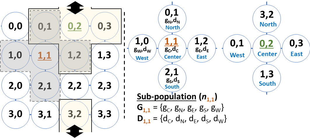
a) Toroidal grid (neighborhood radius: 1) used by Lipizzaner.

b) Ring topology (neighborhood radius: 1).

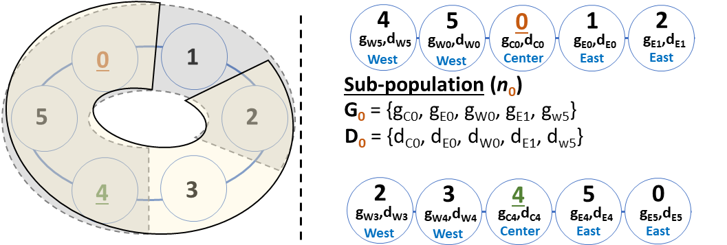
c) Ring topology (neighborhood radius: 2).

Figure 1. Overlapping neighborhoods and sub-population definitions according topologies and neighborhood radius.

Figure 1.a shows an example of a 2D toroidal grid with $Z$=16 (4$\times$4 grid). The shaded areas illustrate the overlapping neighborhoods of the (1,1) and (0,2) cells, with dotted and solid outlines, respectively. The updates in the center of (1,1) will be propagated to the (0,1), (2,1), (1,0), and (1,2) cells.

In Lipi-Ring, the cells are distributed in a one-dimensional grid of size $1\times Z$ and neighbors are sideways, e.g. left and/or right, i.e. an index position or more away. The best GAN (center) after an evolutionary epoch at a cell is updated. Neighborhood cells retrieve this update when they refresh their sub-population membership at the end of their training epochs, effectively forming two non-ending pathways, around the ring, carrying signals in two directions. Figures 1.b and 1.c show populations of six individuals ($Z$=6) organized in a ring topology with neighborhood radius one ($r$=1) and two ($r$=2), respectively. The shaded areas illustrate the overlapping neighborhoods of the cells (0) and (4), with dotted and solid outlines, respectively. The updates in the center of (0) will be propagated to the (5) and (1) for $r$=1 (Figure 1.b) and to the (4), (5), (1), and (2) for $r$=2 (Figure 1.c).

Thus the topologies of Lipizzaner and Lipi-Ring influence communication (of the parameters of the best cell each epoch) and this, in turn, affects how the populations converge.

3.2. Spatially Distributed GAN Training

Algorithm 1 illustrates the main steps of the applied training algorithm. First, it starts the parallel execution of the training on each cell by initializing their own learning hyperparameters (Line 2). Then, the training process consists of a loop with two main phases: first, migration, in which the cells gather the GANs (neighbors) to build the sub-population ($n$), and second, train and evolve when each cell updates the center by applying the coevolutionary GANs training, (see Algorithm 2). These steps are repeated $T$ (generations or training epochs) times. After that, each cell learns an ensemble of generators by using an Evolutionary Strategy, ES-(1+1) (Loshchilov, 2013, Algorithm 2.1), to compute the mixture weights $\omega$ to optimize the accuracy of the generative model returned $(n,\omega)^{*}$ (Schmiedlechner et al., 2018).

For each training generation, the cells apply the CEA in Algorithm 2 in parallel. The CEA starts by selecting best pair generator and discriminator (called $g_{b}$ and $d_{b}$) according to a tournament selection of size $\tau$. It applies an all-vs-all strategy to evaluate all the GAN pairs in the sub-population according to a randomly chosen batch of data $Br$ (Lines 1 to 4). Then, for each batch of data in the training dataset (Lines 5 to 10), the learning rate $n_{\delta}$ is updated applying Gaussian Mutation (Schmiedlechner et al., 2018) and the offspring is created by training $g_{b}$ and $d_{b}$ against a randomly chosen discriminator and generator from the sub-population (i.e., applying gradient-based mutations). Thus, the sub-populations are updated with the new individuals. Finally, a replacement procedure is applied to remove from the sub-populations the weakest individuals and the center is updated with the individuals with the best fitness (Lines 11 to 15). The fitness $\mathcal{L}_{g,d}$ of a given generator (discriminator) is evaluated according to the binary-cross-entropy loss, where the model’s objective is to minimize the Jensen-Shannon divergence between the real and fake data (Goodfellow et al., 2014).

Algorithm 1 Lipizzaner main steps.
Input: T: Total generations, $E$: Grid cells, $s$: Neighborhood size, $\theta_{D}$: Training dataset, $\theta_{COEV}$: Parameters for CoevGANsTraining, $\theta_{EA}$: Parameters for MixtureEA
Return:  $n$: neighborhood,  $\omega$: mixture weights

1:parfor $c\in E$ do $\triangleright$ Asynchronous parallel execution of all cells in grid

2:    $n,\omega\leftarrow$ initializeCells($c,k,\theta_{D}$) $\triangleright$ Initialization of cells

3:    for generation do $\in[0,\dots,\text{T}]$ $\triangleright$ Iterate over generations

4:         $n\leftarrow$ copyNeighbours($c,k$) $\triangleright$ Collect neighbor cells

5:         $n\leftarrow$ CoevGANsTraining ($n,\theta_{D},\theta_{COEV}$) $\triangleright$ Coevolve GANs     

6:    $\omega\leftarrow$ MixtureEA($\omega,n,\theta_{EA}$)$\triangleright$ Build optimal ensemble

7:end parfor

8:return $(n,\omega)^{*}$ $\triangleright$ Cell with best generator mixture

Algorithm 2 CoevGANsTraining
Input: $n$: Cell neighborhood subpopulation, $\theta_{D}$ : Training dataset,  $\tau$ : Tournament size,  $\beta$ : Mutation probability
Return:  $n$ : Cell neighborhood subpopulation trained

1:$Br\leftarrow$ getRandomBatch($\theta_{D}$) $\triangleright$ Random batch to evaluate GAN pairs

2:for $g,d\in\mathbf{g}\times\mathbf{d}$ do $\triangleright$ Evaluate all GAN pairs

3:    $\mathcal{L}_{g,d}\leftarrow$ evaluate($g,d,Br$) $\triangleright$ Evaluate GAN

4:$g_{b},d_{b}\leftarrow$ select($n,\tau$) $\triangleright$ Tournament selection

5:for $B\in\theta_{D}$ do $\triangleright$ Loop over the batches in $\theta_{D}$

6:    $n_{\delta}\leftarrow$ mutateLearningRate($n_{\delta},\beta$) $\triangleright$ Update own $n_{\delta}$

7:    $d\leftarrow$ getRandomOpponent($\mathbf{d}$) $\triangleright$ Get random discriminator

8:    $g_{b}\leftarrow$ updateNN($g_{b},d,B$) $\triangleright$ Update $g_{b}$ with gradient

9:    $g\leftarrow$ getRandomOpponent($\mathbf{g}$) $\triangleright$ Get uniform random generator

10:    $d_{b}\leftarrow$ updateNN($d_{b},g,B$) $\triangleright$ Update $d_{b}$ with gradient

11:$\mathbf{g},\mathbf{d}\leftarrow$ updatePopulations($\mathbf{g}$, $\mathbf{d}$, $g_{b}$, $d_{b}$) $\triangleright$ Add $g_{b}$ and $d_{b}$

12:for $g,d\in\mathbf{g}\times\mathbf{d}$ do $\triangleright$ Evaluate all updated GAN pairs

13:    $\mathcal{L}_{g,d}\leftarrow$ evaluate($g,d,Br$) $\triangleright$ Evaluate GAN

14:$n\leftarrow$ replace($n,\mathbf{g},\mathbf{d}$) $\triangleright$ Replace the networks with worst loss

15:$n\leftarrow$ setCenter($n$) $\triangleright$ Best gen. and disc. are placed in the center

16:return $n$

Here, we have summarized the spatially distributed method applied. More detailed definitions of this spatially distributed GAN training method can be found in (Al-Dujaili et al., 2018; Schmiedlechner et al., 2018).

3.3. Lipi-Ring vs. Lipizzaner

The population structured in a ring with $r$=2 provides a signal propagation similar to the Lipizzaner toroidal grid because both topologies and migration models allow the center individual to reach four cells (two located in the West and two in the East in the case of this ring), see figures 1.a and  1.b. Thus, they provide the same propagation speed and, as their sub-populations are of size $s$=5, the same selection pressure. The signal propagation of the ring with $r$=1 is slower because, after a given training step, the center only reaches two cells (the one in the West and the one in the East), see Figure 1.b. In this case, the sub-populations have three individuals, which reduces the diversity in the sub-population and accelerates convergence (it has 40% fewer individuals than Lipizzaner sub-populations). Thus, Lipi-Ring with $r$=1 reduces the propagation speed, while accelerating the population’s convergence.

Lipi-Ring with $r$=1 has two main advantages over Lipizzaner: a) it mitigates the overhead due to the communication is carried out only with two cells (instead of four) and the sub-populations are smaller, which reduces the number of operations for fitness evaluation and selection/replacement; and b) like all Lipi-Ring with any radius, it does not require to have a rectangular grid of cells, but $Z$ may be any natural number.

Given the infeasibility of analyzing the change in selection and other algorithm elements, we proceed empirically.

4. Experimental setup

We evaluate different distributed CEA GAN training on image data sets: the well known, MNIST (Deng, 2012) and CelebA (Liu et al., 2015); and a dataset of chest X-ray images of patients with COVID-19 (Cohen et al., 2020).

In our experiments, we evaluate the following algorithms: Lipizzaner; two variations of Lipi-Ring both with $r$=1, Ring(1) that performs the same training epochs than Lipizzaner and Ring^t(1) that runs for the same computational cost (wall clock time) than Lipizzaner; and Ring(2) which is the Lipi-Ring with $r$=2 performing the same number of iterations than Lipizzaner. These represent a variety of topologies and migration models. Ring^t(1) is analyzed to make a proper comparison between Ring(1) ($r$=1) and Lipizzaner taking into account the computational cost (time). Table 1 summarizes the main characteristics of the Lipi-Ring variations studied.

The parameters are set according to the authors of Lipizzaner (Schmiedlechner et al., 2018; Toutouh et al., 2019). Thus, all these CEAs apply a tournament selection of size two. The main settings used for the experiments are summarized in Table 2.

Table 1. Lipi-Ring variations analyzed.

Method	$r$	$s$	Variation
Ring(1)	1	3	Same number of iterations as 2D Lipizzaner
Ringt(1)	1	3	Same computational time as 2D Lipizzaner
Ring(2)	2	5	Same number of iterations as 2D Lipizzaner

Table 2. Main GAN training parameters.

Parameter	MNIST	CelebA	COVID-19
Network topology
Network type	MLP	DCGAN	DCGAN
Input neurons	64	100	100
Number of hidden layers	2	4	4
Neurons per hidden layer	256	16,384 - 131,072	32,768 - 524,288
Output neurons	784	64$\times$64$\times$64	128$\times$128
Activation function	$tanh$	$tanh$	$tanh$
Training settings
Batch size	100	128	69
Skip N disc. steps	1	-	-
Learning rate mutation
Optimizer	Adam	Adam	Adam
Initial learning rate	0.0002	0.00005	0.0002
Mutation rate	0.0001	0.0001	0.0001
Mutation probability	0.5	0.5	0.5

For MNIST experiments, the generators and the discriminators are multilayer perceptrons (MLP). The stop condition of each method is defined as follows: a) Ring(1), Ring(2), and Lipizzaner perform 200 training epochs to evaluate the impact of the topology on the performance and computational time required; and b) Ring^t(1) stops after running for the same time than Lipizzaner to compare the methods taking into account the same computational cost (time). The population sizes are 9, 16, and 25, which means Lipizzaner uses grid of sizes 3$\times$3, 4$\times$4, and 5$\times$5. Besides, we study the impact of the size of the populations on Ring(1) by training rings of size between 2 and 9.

For CelebA and COVID-19 experiments, deep convolutional GANs (DCGAN) are trained. DCGANs have much more parameters than MLP (see Table 2). Here, we compare Ring(1) and Lipizzaner. They stop after performing 20 training epochs for CelebA and 1,000 for COVID-19 (because COVID-19 training dataset has much fewer samples). This will discern the differences in terms of performance and computational cost with more complex networks. In these cases, the population size is 9.

The experimental analysis is performed on a cloud computation platform that provides 16 Intel Xeon cores 2.8GHz with 64 GB RAM and an NVIDIA Tesla P100 GPU with 16 GB RAM. We run multiple independent runs for each method.

We have implemented all variations of the Lipi-Ring by extending Lipizzaner framework (Schmiedlechner et al., 2018) using Python and Pytorch (Paszke et al., 2019).

5. Results and discussion

This section presents the results and the analyses of the presented GAN training methods. The first subsections evaluate them with the MNIST dataset. They are measured in terms of: the FID score, the diversity of the generated samples by evaluating the total variation distance (TVD) (Li et al., 2017), and the diversity in the genome space (network parameters). Then, we analyze the CelebA and COVID-19 results with measurements of Inception Score (IS) and computational time. The next subsection presents the results incrementally increasing the ring size of Ring(1). Finally, we compare the computational times needed by Ring(1) and Lipizzaner.

5.1. Quality of the MNIST Generated Data

Table 3 shows the best FID value from each of the 30 independent runs performed for each method. All the evaluated methods improve their performance when increasing the population size, while maintaining the same budget. This could be explained by diversity increasing during the training, as the populations get bigger.

Ring^t(1) has the lowest (best) median and mean FID results. In turn, it returned the generative model that provided the best quality samples (minimum FID score) for all the evaluated population sizes. The second best results are provided by Ring(1). This indicates that the methods with smaller sub-populations converge faster, even though the ring migration model ($r$=1) slows down the propagation of the best individuals.

Table 3. FID MNIST results in terms of best mean, standard deviation, median, interquartile range (Iqr), minimum, and maximum. Best values in bold. (Low FID indicates better samples)

Method	Mean$\pm$Std	Median	Iqr	Min	Max
Population size: 9
Ring(1)	35.45$\pm$6.74	35.02	7.66	22.16	51.09
Ringt(1)	33.42$\pm$5.94	32.83	6.59	22.01	50.56
Ring(2)	42.61$\pm$6.74	42.67	8.70	33.44	58.90
Lipizzaner	40.43$\pm$6.41	40.33	10.37	30.00	52.04
Population size: 16
Ring(1)	29.33$\pm$4.56	28.70	5.93	22.66	40.12
Ringt(1)	27.66$\pm$4.31	27.30	2.23	17.38	39.03
Ring(2)	32.02$\pm$5.86	31.63	9.63	20.52	43.76
Lipizzaner	31.84$\pm$7.26	30.80	6.77	19.15	52.51
Population size: 25
Ring(1)	26.47$\pm$3.88	26.19	5.94	18.41	34.55
Ringt(1)	25.12$\pm$4.65	24.54	5.84	16.65	39.89
Ring(2)	28.01$\pm$4.04	28.84	2.90	19.77	34.92
Lipizzaner	28.81$\pm$4.86	28.14	7.32	22.56	40.57

Comparing Ring(2) and Lipizzaner, they provide close results. Though they use different topologies, their signal propagation and selection operate equally.

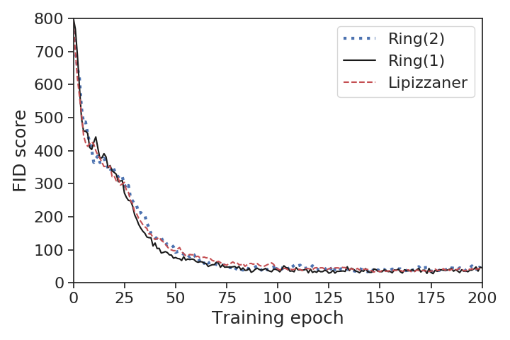
a) Population size: 9

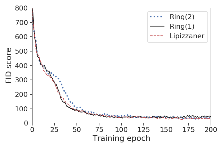
b) Population size: 16

c) Population size: 25

Figure 2. Median FID evolution.

As the results do not follow a normal distribution, we rank the studied methods using the Friedman rank statistical test and we apply Holm correction post-hoc analysis to asses the statistical significance. For all the population sizes, the Friedman ranks Ring^t(1), Lipi-Ring, Lipizzaner, and Ring(2) as the firsts, second, third, and fourth, respectively. However, the significance (p-value) varies from p-value=5.67$\times$10^-6 for population size 9 to p-value=1.13$\times$10^-2 (i.e., p-value$\geq$0.01) for population sizes 16 and 25. According to the Holm post-hoc analysis, Ring(1) and Ring^t(1) are statistically better than Ring(2) and Lipizzaner (which have no statistical differences between each other) for population size 9. For the other population sizes, Ring^t(1) provides statistically better results than Ring(2) and Lipizzaner and there is no significant difference among Ring(1), Ring(2), and Lipizzaner.

Table 3 shows Ring^t(1) is better than Ring(2) and Lipizzaner (lower FID is better). However, the difference between their FIDs decreases when population size increases. This indicates that migration modes that allow faster propagation take better advantage of bigger populations.

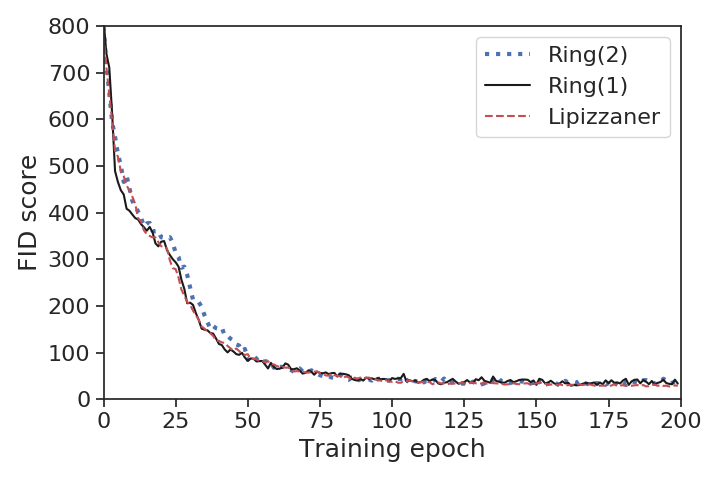
Next, we evaluate the FID score throughout the GAN training process. Figure 2 illustrates the changes of the median FID during the training process. Ring^t(1) is not included because it operates the same as Ring(1).

According to Figure 2, none of the evolutionary GAN training methods seem to have converged. Explaining this will be left to future work. The FID score almost behaves like a monotonically decreasing function with oscillations. The methods with larger sub-populations, i.e., Ring(2) and Lipizzaner, show smaller oscillations which implies more robustness (less variance).

Focusing on the methods with a ring topology, we clearly see the faster convergence when $r$=1. Ring(1) most of the time provides smaller FID values than Ring(2). The reduced sub-population ($s$=3) favors the best individual from the sub-population to be selected during the tournament (it increases the selection pressure).

Figure 2 shows Ring(1), Ring(2), and Lipizzaner converge to similar values. This is in accordance with the results in Table 3 that indicate these three methods provide comparable FID scores.

Finally, Figure 3 illustrates some samples synthesized by generators trained using populations of size 16. As it can be seen, the four sets of samples show comparable quality.

a) Ring(1) MNIST samples

b) Ring^t(1) MNIST samples

c) Ring(2) MNIST samples

d) Lipizzaner MNIST samples

Figure 3. MNIST samples synthesized by generators trained using population size 16.

5.2. Diversity of the Generated MNIST Outputs

This section evaluates the diversity of the samples generated by the best generative models obtained each run. Table 4 reports the TVD for each method and population size. Recall we prefer low TVDs (high diversity) to show the quality of the generative model.

Table 4. TVD MNIST results in terms of best mean, standard deviation, Iqr, minimum, and maximum. Best values in bold. (Low TVD indicates more diverse samples).

Method	Mean$\pm$Std	Median	Iqr	Min	Max
Population size: 9
Ring(1)	0.11$\pm$0.02	0.11	0.03	0.07	0.16
Ringt(1)	0.11$\pm$0.02	0.11	0.03	0.07	0.14
Ring(2)	0.12$\pm$0.02	0.12	0.02	0.09	0.19
Lipizzaner	0.12$\pm$0.02	0.12	0.03	0.08	0.18
Population size: 16
Ring(1)	0.09$\pm$0.02	0.09	0.02	0.07	0.13
Ringt(1)	0.10$\pm$0.01	0.09	0.03	0.07	0.12
Ring(2)	0.10$\pm$0.01	0.10	0.02	0.06	0.13
Lipizzaner	0.10$\pm$0.02	0.10	0.02	0.05	0.16
Population size: 25
Ring(1)	0.09$\pm$0.02	0.09	0.02	0.05	0.12
Ringt(1)	0.09$\pm$0.02	0.09	0.02	0.05	0.11
Ring(2)	0.09$\pm$0.02	0.09	0.01	0.06	0.12
Lipizzaner	0.09$\pm$0.02	0.10	0.02	0.06	0.16

The results in Table 4 demonstrate that, as the population size increases, the resulting trained generative models are able to provide more diverse samples, that is, they have better coverage of the latent distribution. Thus, again, all the methods take advantage bigger populations.

For population size 9, the mean and median TVD of Ring(1) and Ring^t(1) are the lowest. According to Friedman ranking Ring^t(1), Ring(1), Lipizzaner, and Ring(2) are first, second, third, and fourth, respectively (p-value=0.0004). The Holm post-hoc correction confirms that there are no significant differences between Ring(1) and Ring^t(1) and they are statistically more competitive than Ring(2) and Lipizzaner (p-values$<$0.01).

For bigger populations, the statistical analyses report that there are no significant differences between the Ring(1), Ring(2), and Lipizzaner, and Ring^t(1) is statistically better than Ring(2) and Lipizzaner (p-values$<$0.01).

With the support of the FID and TVD results, we can answer RQ1: What is the effect on the generative model trained when changing the directionality of the signal propagation from four directions to two? Answer: The impact on the results of performing migration to one or more neighbors is higher than the directionality itself. If we isolate the directionality, i.e., Lipi-Ring vs. Lipizzaner, the main differences are revealed when $r$=1. Thus, Ring^t(1) generators creates statistically better samples (FID and TVD results) than Lipizzaner. However, when $r$=2, there is no significant difference between Ring(2) and Lipizzaner for all the evaluated population sizes. So, we observe that directionality is irrelevant.

We can also answer RQ2: When the signal is propagated to only two directions, what is the impact of performing migration in one or more neighbors? Answer: When comparing between Lipi-Ring with $r$=1 and with $r$=2 using the same number of training epochs (i.e., Ring(1) and Ring(2)), they perform the same although Ring(1) converges faster. The smallest sub-population of Ring(1) likely increases the selection pressure and the convergence speed of the sub-populations, despite slower signal propagation.

a) Ring(1) (9)

b) Ring^t(1) (9)

c) Ring(2) (9)

c) Lipizzaner (9)

a) Ring(1) (16)

b) Ring^t(1) (16)

c) Ring(2) (16)

c) Lipizzaner (16)

Figure 4. Diversity in genome space. Heatmap of $L_{2}$ distance between the generators for the population size 9 and 16 on MNIST at the end. X and Y axis show cell id. Dark indicates high distance.

5.3. Genome Diversity of MNIST

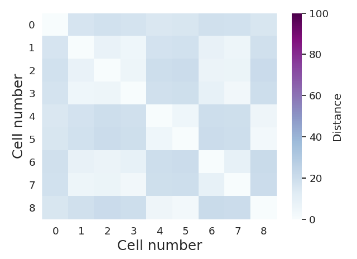
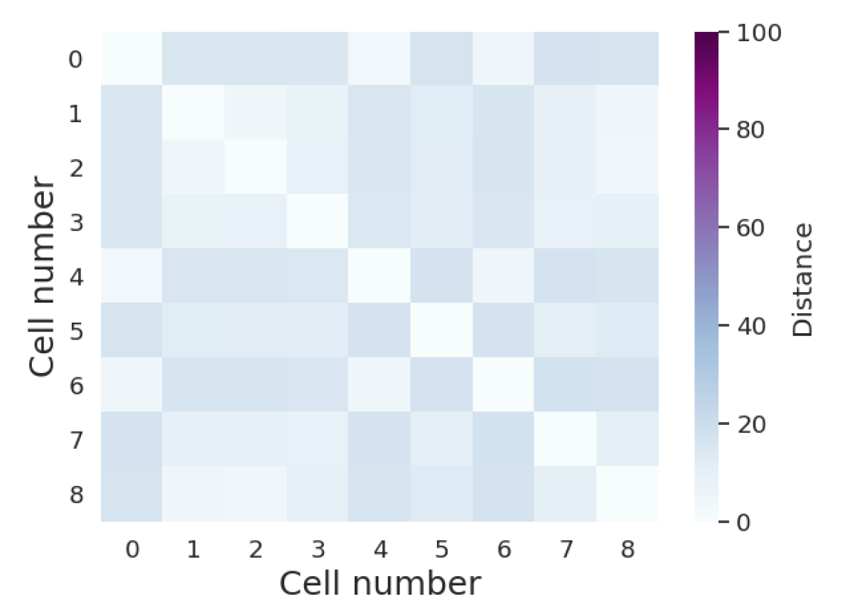
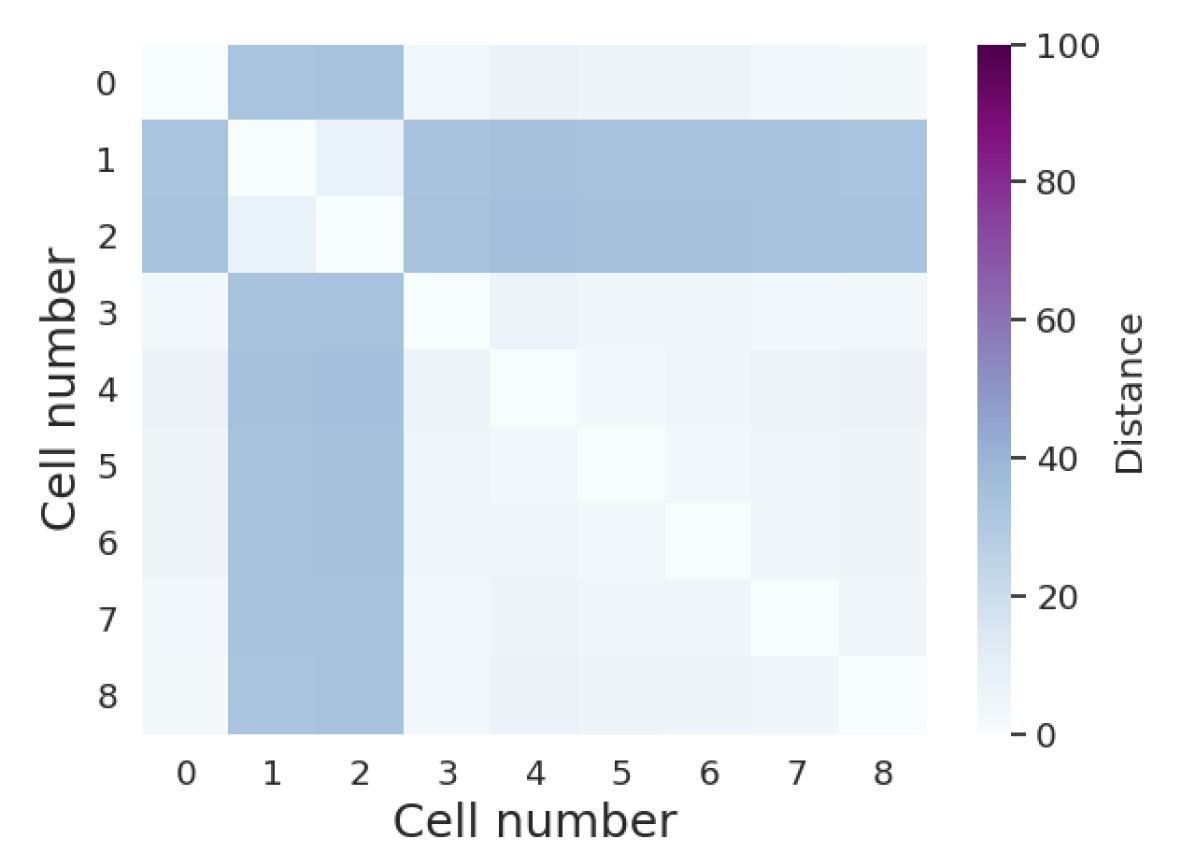
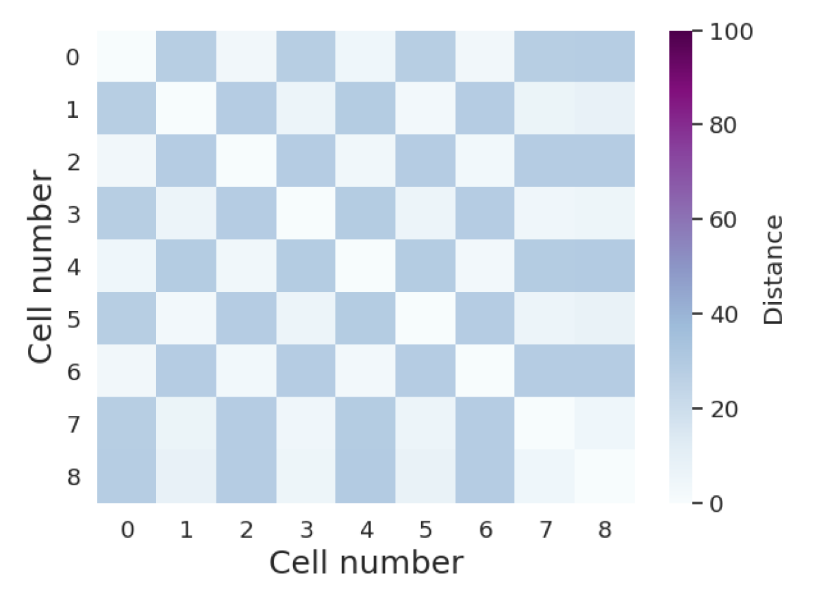
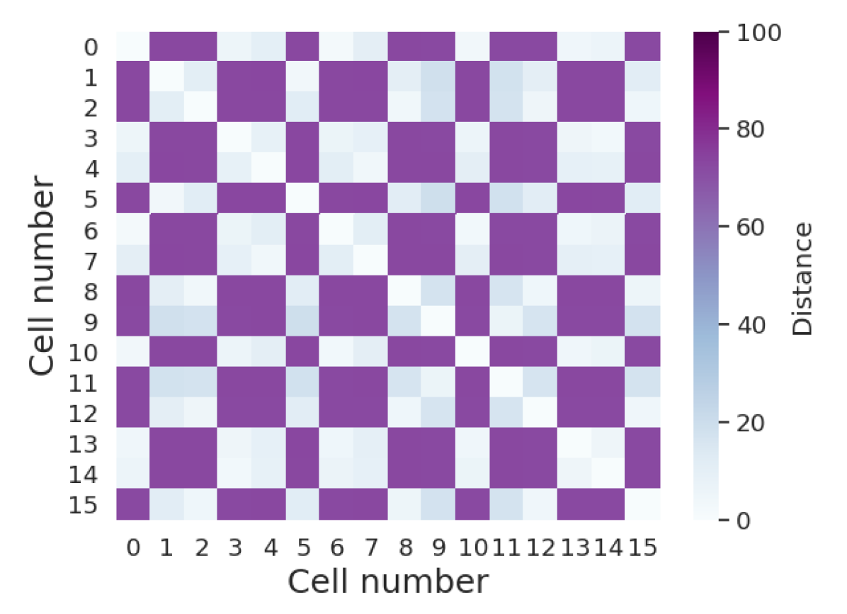
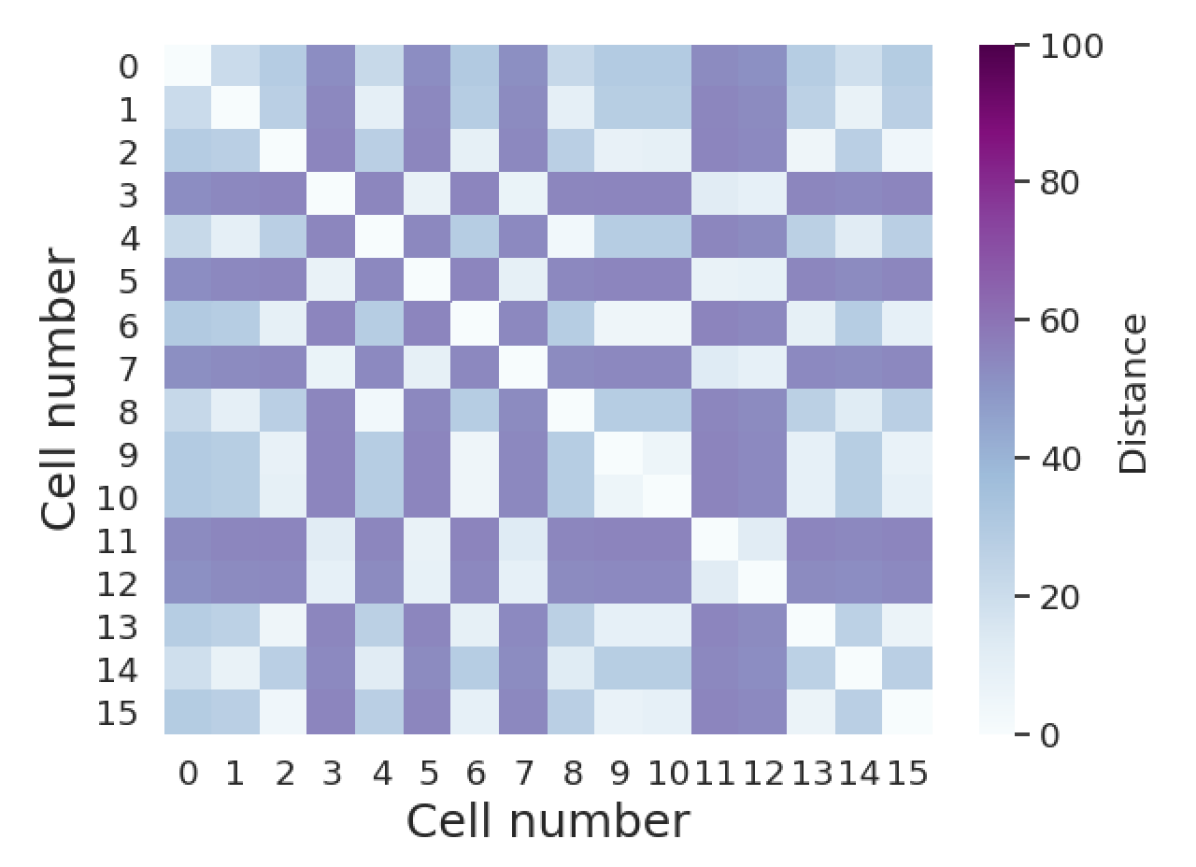
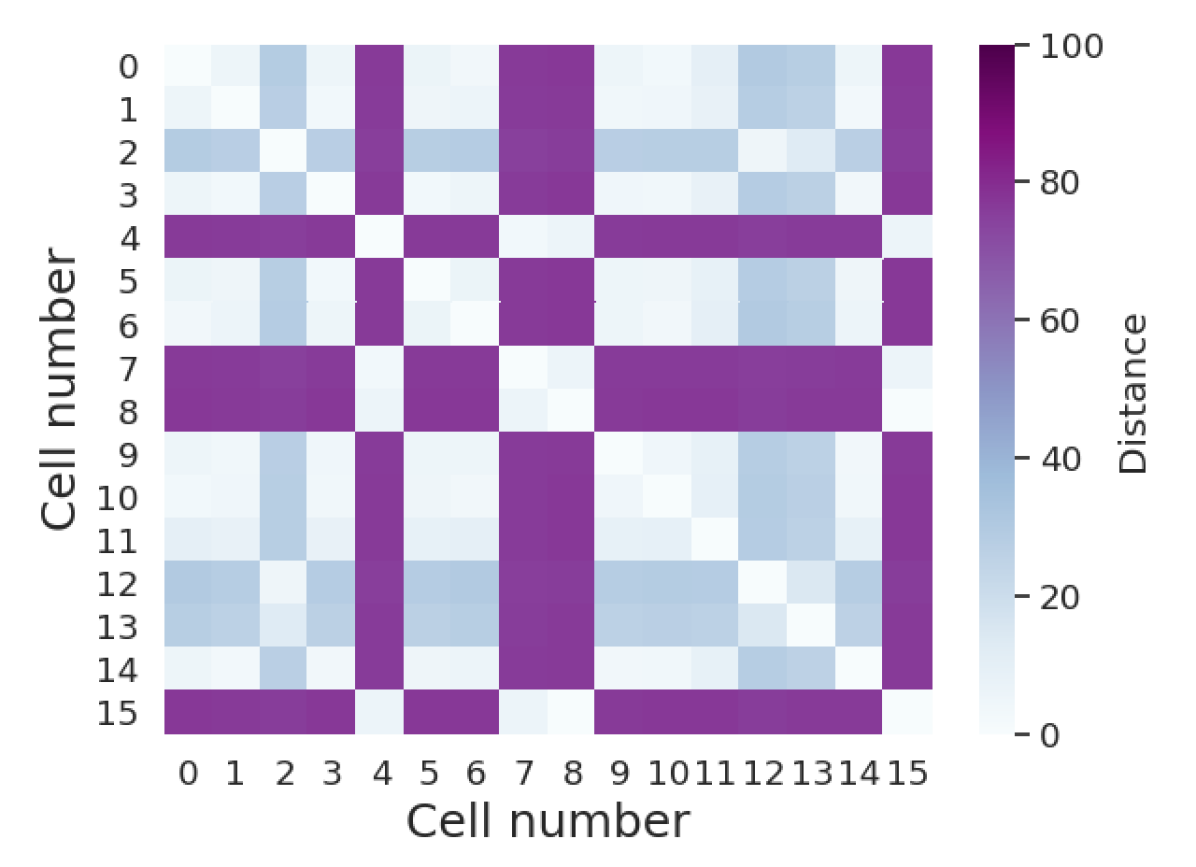
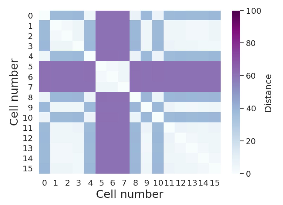
This section analyzes the diversity in the genome space (i.e., the distance between the weights of the evolved networks). We evaluate the populations of size 9 and 16 to see how the migration model and sub-population size affect their diversity. $L_{2}$ distance between neural network parameters in a given population is used to measure diversity and Table 5 summarizes the results. Figure 4 presents the $L_{2}$ distances for the populations that represent the median $L_{2}$.

Table 5. $L_{2}$ distance values between the weights of the networks in different cells on MNIST dataset. High values indicates more networks diversity. Highest value is in bold.

Method	Mean$\pm$Std	Median	Iqr	Min	Max
Population size: 9
Ring(1)	16.92$\pm$7.14	15.53	9.60	6.79	40.19
Ringt(1)	13.38$\pm$4.97	12.07	6.49	6.67	22.56
Ring(2)	12.69$\pm$5.89	13.98	10.85	4.10	23.33
Lipizzaner	13.85$\pm$8.29	18.06	15.32	4.09	23.46
Population size: 16
Ring(1)	36.12$\pm$18.72	34.21	30.32	13.44	70.28
Ringt(1)	34.88$\pm$13.33	32.62	10.30	17.75	66.18
Ring(2)	32.44$\pm$21.10	21.97	25.90	11.31	86.03
Lipizzaner	30.99$\pm$24.28	28.09	55.82	2.72	61.34

Focusing on the Lipi-Ring methods with $r$=1, the population diversity diminishes with more training, i.e., $L_{2}$ distances between the networks in Ring(1) are higher than in Ring^t(1) for both population sizes, see Table 5 and Figure 4. This shows that as the ring runs longer the genotypes are starting to converge.

Taking into account the Lipi-Ring methods with $r$=1 and $r$=2 that performed the same number of training epochs, i.e., Ring(1) and Ring(2), the first one shows higher $L_{2}$ distances (darker colors in Figure 4). This confirms that the populations are more diverse when signal propagation is slower.

Comparing Ring(2) and Lipizzaner, that have the same sub-population size and migration to four neighbors, there is not a clear trend because Lipizzaner generated more diverse populations for population size 9 and Ring(2) for population size 16. Therefore, we have not found a clear effect of changing the migration from four to two directions.

According to these results, we can answer the questions formulated in RQ3. How does diversity change over time in a ring topology? When Ring(1) performs more training the diversity decreases. How does diversity compare with a ring topology with different neighborhood radius? As the radius increases, the diversity is lower because the propagation of the best individuals is faster. How does diversity compare between ring topology and 2D grid, where both methods have the same sub-population size and neighborhood, but different signal directionality? We have not proven any clear impact on the diversity when changing the directionality for the methods that have the same sub-population size and neighborhood.

5.4. CelebA and COVID-19

According to the empirical results, in general, Ring(1) and Lipizzaner compute generative models with comparable quality for MNIST (training MLP networks). Here, we study both methods training generative models for generating synthesized samples of CelebA and COVID-19 datasets using convolutional DNN, which are bigger networks (having more parameters). Table 6 shows the best IS value from each of the 10 independent runs for each method with population size 9.

In this case, it is more clear that both methods demonstrated the same performance. Focusing on CelebA dataset, Ring(1) computes higher (better) mean, minimum, and maximum IS, but Lipizzaner shows higher median. For the COVID-19 dataset, Lipizzaner shows better mean, median, and maximum IS values. The statistical analysis (ANOVA test) corroborates that there is not significant differences between both methods for both datasets (i.e., CelebA p-value=3.049 and COVID-19 p-value=0.731).

Table 6. IS results in terms of best mean, standard deviation, median, Iqr, minimum, and maximum for CelebA and COVID-19 experiments. Best values in bold. (High IS indicates better samples)

Method	Mean$\pm$Std	Median	Iqr	Min	Max
Dataset: CelebA
Ring(1)	36.61$\pm$1.95	35.94	2.31	34.40	40.40
Lipizzaner	36.30$\pm$1.77	36.34	2.86	32.95	39.02
Dataset: COVID-19
Ring(1)	1.79$\pm$0.12	1.79	0.20	1.63	2.00
Lipizzaner	1.86$\pm$0.19	1.84	0.16	1.61	2.24

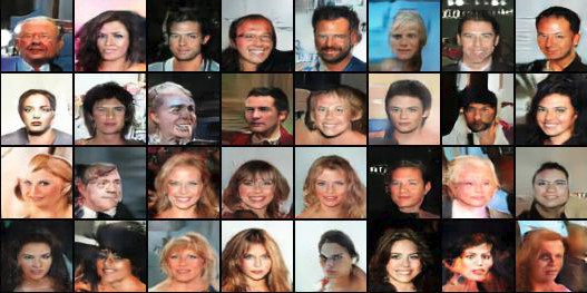
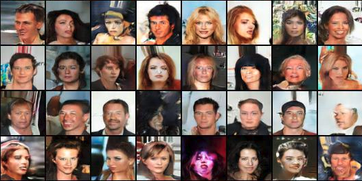
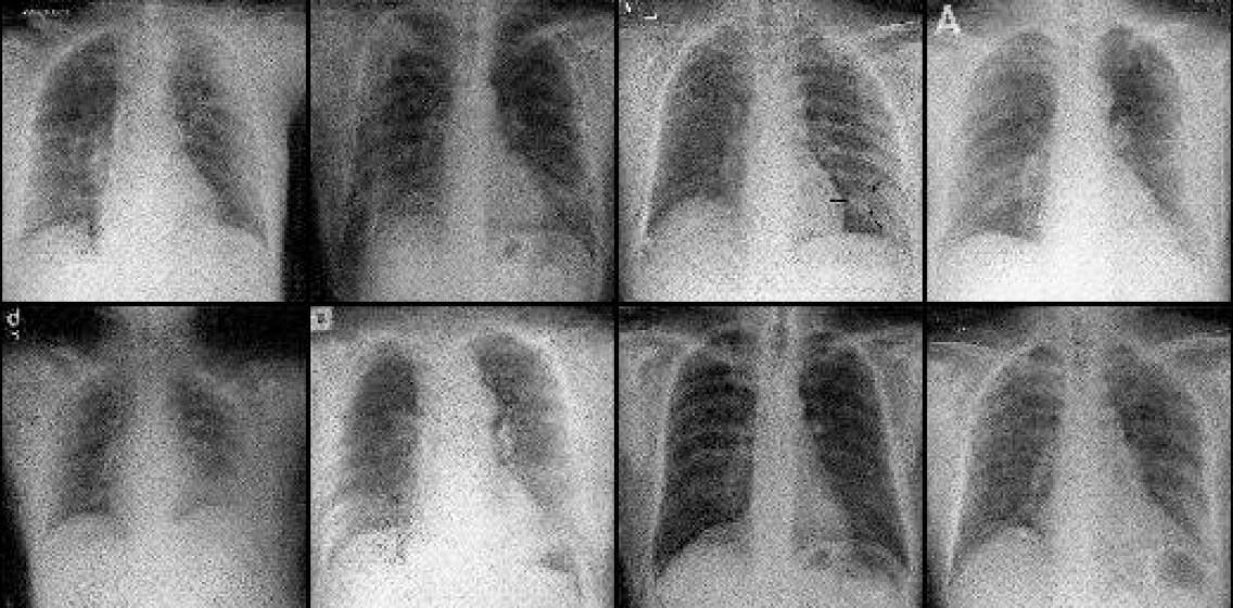
Finally, Figure 5 illustrates some samples of CelebA and COVID-19 synthesized by the generators trained using Ring(1) and Lipizzaner. As it can be seen, the samples show similar quality.

a) Ring(1)- CelebA

b) Lipizzaner- CelebA

c) Ring(1)- COVID-19

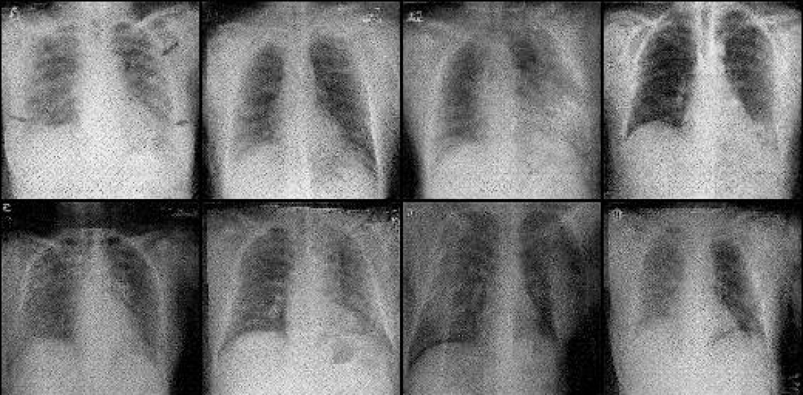
d) Lipizzaner- COVID-19

Figure 5. Samples of CelebA and COVID-19 synthesized by generators trained using Ring(1) and Lipizzaner.

Note that these results are in the line of the answers given to RQ1 and RQ2. The change of directionality of the signal propagation and of the migration model allows the method to achieve the same results as Lipizzaner.

5.5. Lipi-Ring Scalability Analysis

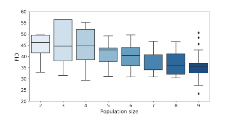
Here, we evaluate the results incrementally increasing the ring size of Ring(1) from 2 to 9 using MNIST dataset. Figure 6 illustrates how increasing the population size of Ring(1) by only one individual improves the result (reduces the FID). However, Lipizzaner using, an a$\times$b 2D-grid would require adding (at least) $a$ or $b$ individuals.

Figure 6. FID MNIST results according to the population size.

5.6. Computational Time Comparisons

We know that training with smaller sub-populations sizes takes shorter times because it performs fewer operations. As the reader may be curious about the time savings of using Ring(1) instead of Lipizzaner, we compare their computational times for the experiments performed. Notice that they perform the same number of training epochs (see Section 4) and provide comparable quality results. Table 7 summarizes the computational cost in wall clock time for all the methods, population sizes, and datasets. All the analyzed methods have been executed on a cloud architecture, which could generate some discrepancies.

Table 7. Computational time cost in terms of mean and standard deviation (minutes).

MNIST
Population size	9	16	25
Ring(1)	65.83$\pm$1.02	72.95$\pm$0.22	92.42$\pm$1.82
Lipizzaner	87.86$\pm$1.28	91.19$\pm$1.80	105.54$\pm$1.98
CelebA		COVID-19
Population size	9	Population size	9
Ring(1)	224.37$\pm$2.36	Ring(1)	118.87$\pm$0.95
Lipizzaner	276.47$\pm$26.36	Lipizzaner	168.57$\pm$0.32

As expected, Ring(1) requires shorter times. Comparing both methods on MNIST, Lipizzaner needed 33.46%, 25.01%, and 14.20% longer times than Ring(1) for population sizes 9, 16, and 25, respectively. This indicates that the computation effort of using 40% bigger sub-populations (5 instead of 3 individuals) affects less the running times as the population size increases.

For CelebA and COVID-19 experiments, Ring(1) reduces the mean computational time by 23.22% in CelebA experiments and by 41.18% in COVID-19. The time saving is higher for COVID-19 mainly because the training methods performed more epochs (1,000) for this dataset than for CelebA (20 epochs). The sub-population size principally affects the required effort to perform the evaluation of the whole sub-population and the selection/replacement operation which are carried out for each training iteration. This explains why the time saving are higher for COVID-19 experiments.

6. Conclusions and future work

The empirical analysis of different spatially distributed CEA GAN training methods shows that the use of a ring topology instead of a 2D grid does not lead to a loss of quality in the computed generative models, but it may improve them (it depends on the setup).

Ring^t(1), which uses a ring topology with neighborhood radius $r$=1 and run for the same time than Lipizzaner, produced the best generative models. Ring(1), Ring(2), and Lipizzaner, which were trained for the same training epochs, trained comparable generative models on the MNIST, CelebA, and COVID-19 datasets (similar FID and TVD for MNIST and IS for CelebA and COVID-19).

In terms of diversity, Ring(1) shows the most diverse populations which diminishes with more training. Focusing on ring topology, when the migration radius increases, i.e., Ring(1) ($r$=1) vs. Ring(2) ($r$=2), the diversity decreases. Finally, we have not found a marked difference on the diversity of the populations when changing the migration directionality , i.e., comparing between Ring(2) and Lipizzaner.

Ring(1), changing the signal propagation from four to two directions and using a migration of radius one, reduced the computational time cost of Lipizzaner by between 14.2% and 41.2%, while keeping comparable quality results.

Future work will include the evaluation of Ring(1) on more datasets, bigger populations, and for longer training epochs. We will apply specific strategies to deal with small sub-populations (3 individuals per cell) to analyze the effect of reducing the high selection pressure. We will perform a convergence analysis to provide appropriate Lipizzaner and Ring(1) setups to address MNIST. Finally, we are exploring new techniques to evolve the network architectures during the CEA training.

References

- (1)
- Al-Dujaili et al. (2018) Abdullah Al-Dujaili, Tom Schmiedlechner, Erik Hemberg, and Una-May O’Reilly. 2018. Towards distributed coevolutionary GANs. In AAAI 2018 Fall Symposium.
- Arjovsky and Bottou (2017) Martin Arjovsky and Léon Bottou. 2017. Towards Principled Methods for Training Generative Adversarial Networks. arXiv e-prints, art. arXiv preprint arXiv:1701.04862 (2017).
- Arjovsky et al. (2017) Martin Arjovsky, Soumith Chintala, and Léon Bottou. 2017. Wasserstein GAN. arXiv preprint arXiv:1701.07875 (2017).
- Arora et al. (2017) Sanjeev Arora, Rong Ge, Yingyu Liang, Tengyu Ma, and Yi Zhang. 2017. Generalization and Equilibrium in Generative Adversarial Nets (GANs). arXiv preprint arXiv:1703.00573 (2017).
- Arora et al. (2018) Sanjeev Arora, Andrej Risteski, and Yi Zhang. 2018. Do GANs learn the distribution? Some Theory and Empirics. In International Conference on Learning Representations. https://openreview.net/forum?id=BJehNfW0-
- Baioletti et al. (2020) Marco Baioletti, Carlos Artemio Coello Coello, Gabriele Di Bari, and Valentina Poggioni. 2020. Multi-objective evolutionary GAN. In Proceedings of the 2020 Genetic and Evolutionary Computation Conference Companion. 1824–1831.
- Cohen et al. (2020) Joseph Paul Cohen, Paul Morrison, and Lan Dao. 2020. COVID-19 image data collection. arXiv 2003.11597 (2020). https://github.com/ieee8023/covid-chestxray-dataset
- Costa et al. (2019) Victor Costa, Nuno Lourenço, and Penousal Machado. 2019. Coevolution of generative adversarial networks. In International Conference on the Applications of Evolutionary Computation (Part of EvoStar). Springer, 473–487.
- Deng (2012) L. Deng. 2012. The MNIST Database of Handwritten Digit Images for Machine Learning Research [Best of the Web]. IEEE Signal Processing Magazine 29, 6 (2012), 141–142. https://doi.org/10.1109/MSP.2012.2211477
- Garciarena et al. (2018) Unai Garciarena, Roberto Santana, and Alexander Mendiburu. 2018. Evolved GANs for generating Pareto set approximations. In Proceedings of the Genetic and Evolutionary Computation Conference. 434–441.
- Goodfellow et al. (2014) Ian Goodfellow, Jean Pouget-Abadie, Mehdi Mirza, Bing Xu, David Warde-Farley, Sherjil Ozair, Aaron Courville, and Yoshua Bengio. 2014. Generative adversarial nets. In Advances in neural information processing systems. 2672–2680.
- Gulrajani et al. (2017) Ishaan Gulrajani, Faruk Ahmed, Martin Arjovsky, Vincent Dumoulin, and Aaron C Courville. 2017. Improved training of Wasserstein GANs. In Advances in neural information processing systems. 5767–5777.
- Jolicoeur-Martineau (2018) Alexia Jolicoeur-Martineau. 2018. The relativistic discriminator: a key element missing from standard GAN. arXiv preprint arXiv:1807.00734 (2018).
- Karras et al. (2017) Tero Karras, Timo Aila, Samuli Laine, and Jaakko Lehtinen. 2017. Progressive growing of GANs for improved quality, stability, and variation. arXiv preprint arXiv:1710.10196 (2017).
- Li et al. (2017) Chengtao Li, David Alvarez-Melis, Keyulu Xu, Stefanie Jegelka, and Suvrit Sra. 2017. Distributional Adversarial Networks. arXiv preprint arXiv:1706.09549 (2017).
- Liu et al. (2015) Ziwei Liu, Ping Luo, Xiaogang Wang, and Xiaoou Tang. 2015. Deep Learning Face Attributes in the Wild. In Proceedings of International Conference on Computer Vision (ICCV).
- Loshchilov (2013) Ilya Loshchilov. 2013. Surrogate-assisted evolutionary algorithms. Ph.D. Dissertation. University Paris South Paris XI; National Institute for Research in Computer Science and Automatic-INRIA.
- Mao et al. (2017) Xudong Mao, Qing Li, Haoran Xie, Raymond YK Lau, Zhen Wang, and Stephen Paul Smolley. 2017. Least squares generative adversarial networks. In Proceedings of the IEEE International Conference on Computer Vision. 2794–2802.
- Nguyen et al. (2017) Tu Nguyen, Trung Le, Hung Vu, and Dinh Phung. 2017. Dual discriminator generative adversarial nets. In Advances in Neural Information Processing Systems. 2670–2680.
- Paszke et al. (2019) Adam Paszke, Sam Gross, Francisco Massa, Adam Lerer, James Bradbury, Gregory Chanan, Trevor Killeen, Zeming Lin, Natalia Gimelshein, Luca Antiga, Alban Desmaison, Andreas Kopf, Edward Yang, Zachary DeVito, Martin Raison, Alykhan Tejani, Sasank Chilamkurthy, Benoit Steiner, Lu Fang, Junjie Bai, and Soumith Chintala. 2019. PyTorch: An Imperative Style, High-Performance Deep Learning Library. In Advances in Neural Information Processing Systems 32, H. Wallach, H. Larochelle, A. Beygelzimer, F. d'Alché-Buc, E. Fox, and R. Garnett (Eds.). Curran Associates, Inc., 8024–8035. http://papers.neurips.cc/paper/9015-pytorch-an-imperative-style-high-performance-deep-learning-library.pdf
- Popovici et al. (2012) Elena Popovici, Anthony Bucci, R Paul Wiegand, and Edwin D De Jong. 2012. Coevolutionary principles. In Handbook of natural computing. Springer, 987–1033.
- Radford et al. (2015) Alec Radford, Luke Metz, and Soumith Chintala. 2015. Unsupervised Representation Learning with Deep Convolutional Generative Adversarial Networks. arXiv preprint arXiv:1511.06434 (2015).
- Salimans et al. (2016) Tim Salimans, Ian Goodfellow, Wojciech Zaremba, Vicki Cheung, Alec Radford, and Xi Chen. 2016. Improved techniques for training GANs. In Advances in neural information processing systems. 2234–2242.
- Schmiedlechner et al. (2018) Tom Schmiedlechner, Ignavier Ng Zhi Yong, Abdullah Al-Dujaili, Erik Hemberg, and Una-May O’Reilly. 2018. Lipizzaner: A System That Scales Robust Generative Adversarial Network Training. In the 32nd Conference on Neural Information Processing Systems (NeurIPS 2018) Workshop on Systems for ML and Open Source Software.
- Toutouh et al. (2019) Jamal Toutouh, Erik Hemberg, and Una-May O’Reilly. 2019. Spatial Evolutionary Generative Adversarial Networks. In Proceedings of the Genetic and Evolutionary Computation Conference (GECCO ’19). ACM, New York, NY, USA, 472–480. https://doi.org/10.1145/3321707.3321860
- Toutouh et al. (2020a) Jamal Toutouh, Erik Hemberg, and Una-May O’Reilly. 2020a. Analyzing the Components of Distributed Coevolutionary GAN Training. In Parallel Problem Solving from Nature – PPSN XVI, Thomas Bäck, Mike Preuss, André Deutz, Hao Wang, Carola Doerr, Michael Emmerich, and Heike Trautmann (Eds.). Springer International Publishing, Cham, 552–566.
- Toutouh et al. (2020b) Jamal Toutouh, Erik Hemberg, and Una-May O’Reilly. 2020b. Data Dieting in GAN Training. Springer Singapore, Singapore, 379–400.
- Toutouh et al. (2020c) Jamal Toutouh, Erik Hemberg, and Una-May O’Reily. 2020c. Re-Purposing Heterogeneous Generative Ensembles with Evolutionary Computation. In Proceedings of the 2020 Genetic and Evolutionary Computation Conference (GECCO ’20). Association for Computing Machinery, New York, NY, USA, 425–434.
- Wang et al. (2019) Chaoyue Wang, Chang Xu, Xin Yao, and Dacheng Tao. 2019. Evolutionary generative adversarial networks. IEEE Transactions on Evolutionary Computation 23, 6 (2019), 921–934.
- Williams and Mitchell (2005) Nathan Williams and Melanie Mitchell. 2005. Investigating the Success of Spatial Coevolution. In Proceedings of the 7th Annual Conference on Genetic and Evolutionary Computation (GECCO ’05). Association for Computing Machinery, New York, NY, USA, 523–530.
- Zhao et al. (2016) Junbo Zhao, Michael Mathieu, and Yann LeCun. 2016. Energy-based generative adversarial network. arXiv preprint arXiv:1609.03126 (2016).