∎
Quantifying the effects of environment and population diversity in multi-agent reinforcement learning
Abstract
Generalization is a major challenge for multi-agent reinforcement learning. How well does an agent perform when placed in novel environments and in interactions with new co-players? In this paper, we investigate and quantify the relationship between generalization and diversity in the multi-agent domain. Across the range of multi-agent environments considered here, procedurally generating training levels significantly improves agent performance on held-out levels. However, agent performance on the specific levels used in training sometimes declines as a result. To better understand the effects of co-player variation, our experiments introduce a new environment-agnostic measure of behavioral diversity. Results demonstrate that population size and intrinsic motivation are both effective methods of generating greater population diversity. In turn, training with a diverse set of co-players strengthens agent performance in some (but not all) cases.
Keywords:
Machine learning Deep reinforcement learning Multi-agent Diversity1 Introduction
An emerging theme in single-agent reinforcement learning research is the effect of environment diversity on learning and generalization juliani2019obstacle ; justesen2018illuminating ; wang2019paired . Reinforcement learning agents are typically trained and tested on a single level, which produces high performance and brittle generalization. Such overfitting stems from agents’ capacity to memorize a mapping from environmental states observed in training to specific actions zhang2018study . Single-agent research has counteracted and alleviated overfitting by incorporating environment diversity into training. For example, procedural generation can be used to produce larger sets of training levels and thereby encourage policy generality cobbe2019leveraging ; cobbe2019quantifying .
In multi-agent settings, the tendency of agents to overfit to their co-players is another large challenge to generalization lanctot2017unified . Generalization performance tends to be more robust when agents train with a heterogeneous set of co-players. Prior studies have induced policy generality through population-based training carroll2019utility ; jaderberg2019human , policy ensembles lowe2017multi , the application of diverse leagues of game opponents vinyals2019grandmaster , and the diversification of architectures or hyperparameters for the agents within the population hu2020other ; mckee2020social .
Of course, the environment is still a major component of multi-agent reinforcement learning. In multi-agent games, an agent’s learning is shaped by both the other co-players and the environment littman1994markov . Despite this structure, only a handful of studies have explicitly assessed the effects of environmental variation on multi-agent learning. Jaderberg et al. jaderberg2019human developed agents for Capture the Flag that were capable of responding to a variety of opponents and match conditions. They argued that this generalizability was produced in part by the use of procedurally generated levels during training. Other multi-agent experiments using procedurally generated levels (e.g., everett2019optimising ; leibo2019malthusian ) stop short of rigorously measuring generalization. It thus remains an open question whether procedural generation of training levels benefits generalization in multi-agent learning.
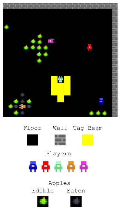
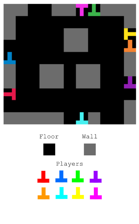
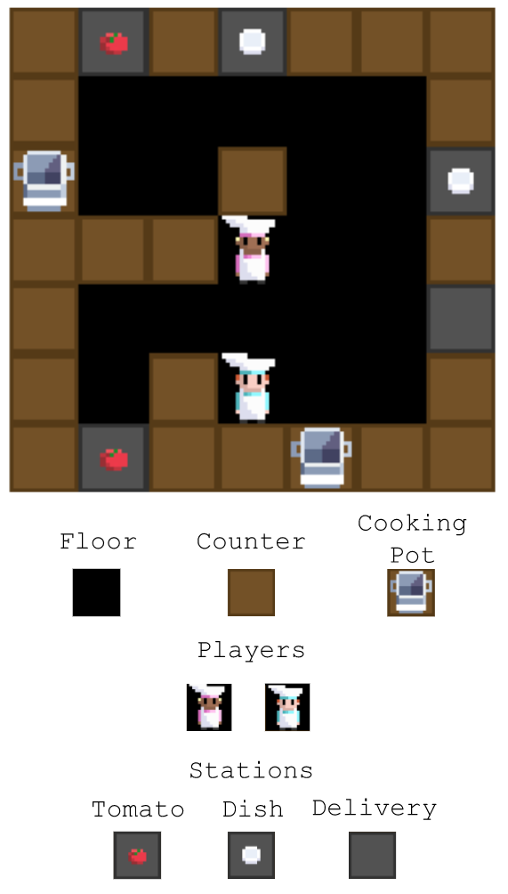
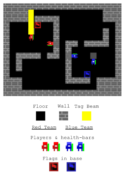
Here we build from prior research and rigorously characterize the effects of environment and population diversity on multi-agent reinforcement learning. Specifically, we use procedural generation and population play to investigate performance and generalization in four distinct multi-agent environments drawn from prior studies: HarvestPatch, Traffic Navigation, Overcooked, and Capture the Flag. These experiments make three contributions to multi-agent reinforcement learning research:
-
1.
Agents trained with greater environment diversity exhibit stronger generalization to new levels. However, in some environments and with certain co-players, these improvements come at the expense of performance on an agent’s training set.
-
2.
Expected action variation—a new, domain-agnostic metric introduced here—can be used to assess behavioral diversity in a population.
-
3.
Behavioral diversity tends to increase with population size, and in some (but not all) environments is associated with increases in performance and generalization.
2 Environments
2.1 Markov games and multi-agent reinforcement learning
This paper aims to explore the influence of diversity on agent behavior and generalization in -player Markov games littman1994markov . A partially observable Markov game is played by players within a finite set of states . The game is parameterized by an observation function , sets of available actions for each player , and a stochastic transition function , mapping from joint actions at each state to the set of discrete probability distributions over states.
Each player independently experiences the game and receives its own observation . The observations of the players in the game can be represented jointly as . Following this notation, we can also refer to the vector of player actions for convenience. Each agent independently learns a behavior policy based on its observation and its extrinsic reward . Agent learns a policy which maximizes a long-term -discounted payoff defined as:
| (1) |
where is the utility function for agent . In the absence of reward sharing ibrahim2020reward or instrinsic motivation hughes2018inequity ; singh2005intrinsically , the utility function maps directly to the extrinsic reward provided by the environment.
A key source of diversity in Markov games is the environment itself. To this end, we train agents on distributions of environment levels produced by procedural generators. Our investigation explores four distinct environments drawn from prior studies: HarvestPatch (a mixed-motive game), Traffic Navigation (a coordination game), Overcooked (a common-payoff game), and Capture the Flag (a competitive game). The following subsections provide an overview of the game rules for each of these games. All environments were implemented with the open-source engine DeepMind Lab2D beattie2020deepmind . Full details on the environments and the procedural generation methods are available in the Appendix A.
2.2 HarvestPatch
HarvestPatch mckee2020social (Figure 1(a)) is a mixed-motive game, played by players in the experiments here (see also hughes2018inequity ; jaques2019intrinsic ; kramar2020should ; perolat2017multi ).
Players inhabit a gridworld environment containing harvestable apples. Players can harvest apples by moving over them, receiving a small reward for each apple collected ( reward). Apples regrow after being harvested at a rate determined by the number of unharvested apples within the regrowth radius . An apple cannot regrow if there are no apples within its radius. This property induces a social dilemma for the players. The group as a whole will perform better if its members are abstentious in their apple consumption, but in the short term individuals can always do better by harvesting greedily.
Levels are arranged with patches of apples scattered throughout the environment in varying densities. Every step, players can either stand still, move around the level, or fire a short tag-out beam. If another player is hit by the beam, they are removed from play for a number of steps. They also observe a partial egocentric window of the environment.
2.3 Traffic Navigation
Traffic Navigation lerer2019learning (Figure 1(b)) is a coordination game, played by players.
Players are placed at the edges of a gridworld environment and tasked with reaching specific goal locations within the environment. When a player reaches their goal, they receive a reward and a new goal location. If they collide with another player, they receive a negative reward. Consequently, each player’s objective is to reach their goal locations as fast as possible while avoiding collisions with other players.
To make coordinated navigation more challenging, blocking walls are scattered throughout the environment, creating narrow paths which limit the number of players that can pass at a time. On each step of the game, players can either stand still or move around the level. Players observe both a small egocentric window of the environment and their relative offset to their current goal location.
2.4 Overcooked
Overcooked carroll2019utility (Figure 1(c)) is a common-payoff game, played in the experiments here by players (see also charakorn2020investigating ; knott2021evaluating ; wang2020too ).
Players are placed in a kitchen-inspired gridworld environment and tasked with cooking as many dishes of tomato soup as possible. Cooking a dish is a sequential task: players must deposit three tomatoes into a cooking pot, let the tomatoes cook, remove the cooked soup with a dish, and then deliver the dish. Both players receive a reward upon the delivery of a plated dish.
Environment levels contain multiple cooking pots and stations. Players can coordinate their actions to maximize their shared reward. On each step, players can stand still, move around the level, or interact with the entity the object are facing (e.g., pick up tomato, place tomato onto counter, or deliver soup). Players observe a partial egocentric window of the level.
2.5 Capture the Flag
Capture the Flag (Figure 1(d)) is a competitive game. Jaderberg et al. jaderberg2019human studied Capture the Flag using the Quake engine. Here, we implement a gridworld version of Capture the Flag played by players.
Players are split into red and blue teams and compete to capture the opposing team’s flag by strategically navigating, evading, and tagging members of the opposing team. The team that captures the greater number of flags by the end of the episode wins.
Walls partition environment levels into rooms and corridors, generating strategic spaces for players to navigate and exploit to gain an advantage over the other team. On each step, players can stand still, move around the level, or fire a tag-out beam. If another player is hit by the tag-out beam three times, they are removed from play for a set number of steps. Each player observes a partial egocentric window oriented in the direction they are facing, as well as whether each of the two flags is held by its opposing team.
3 Agents
We use a distributed, asynchronous framework for training, deploying a set of “arenas” to train each population of reinforcement learning agents. Arenas run in parallel; each arena instantiates a copy of the environment, running one episode at a time. To begin an episode, an arena selects a population of size with an associated set of training levels. The arena samples one level from the population’s training set and agents from the population (with replacement). The episode lasts steps, with the resulting trajectories used by the sampled agents to update their weights. Agents are trained until episodic rewards converge. After training ends, we run various evaluation experiments with agents sampled after the convergence point.
For the learning algorithm of our agents, we use V-MPO song2019v , an on-policy variant of Maximum a Posteriori Policy Optimization (MPO). In later experiments, we additionally endow these agents with the Social Value Orientation (SVO) component, encoding an intrinsic motivation to maintain certain group distributions of reward mckee2020social . These augmented agents act as a baseline for our behavioral diversity analysis, following suggestions from prior research that imposing variation in important hyperparameters can lead to greater population diversity. More details on the algorithm (including hyperparameters) are available in Appendix B.
4 Methods
4.1 Investigating Environment Diversity
To assess how environment diversity (i.e., the number of unique levels encountered during training) affects an agent’s ability to generalize, we follow single-agent work on quantifying agent generalization in procedurally generated environments cobbe2019leveraging ; cobbe2019quantifying ; zhang2018study .
Specifically, we train multiple populations of agents with different sets of training levels. We procedurally generate training levels in sets of size , where each training set is a subset of any larger sets. We also procedurally generate a separate test set containing 100 held-out levels. These held-out levels are not played by agents during training. For each training set of size , we launch ten independent training runs and train each population until their rewards converge.
Generalization Gap
Following prior work, we compare the performance of populations on the levels from their training set with their performance on the 100 held-out test levels. We focus on the size of the generalization gap, defined as the absolute difference between the population’s performance on the test-set levels and training-set levels.
Cross-Play Evaluation
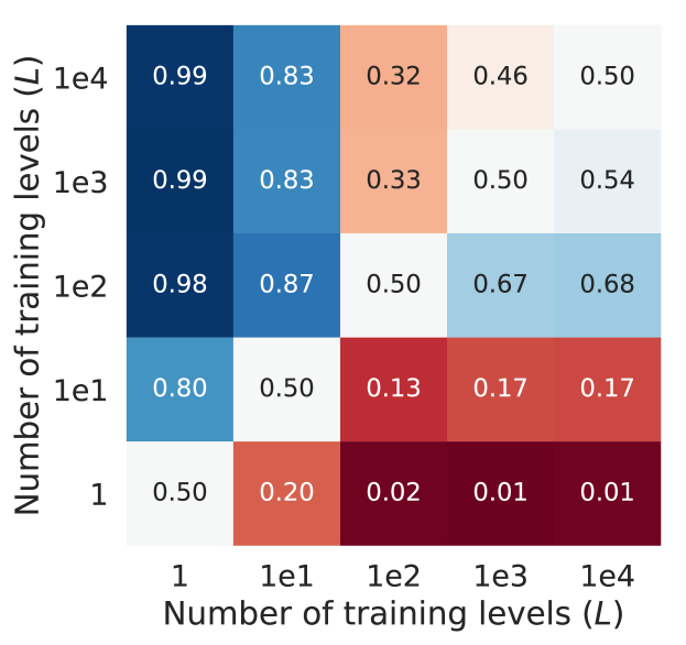
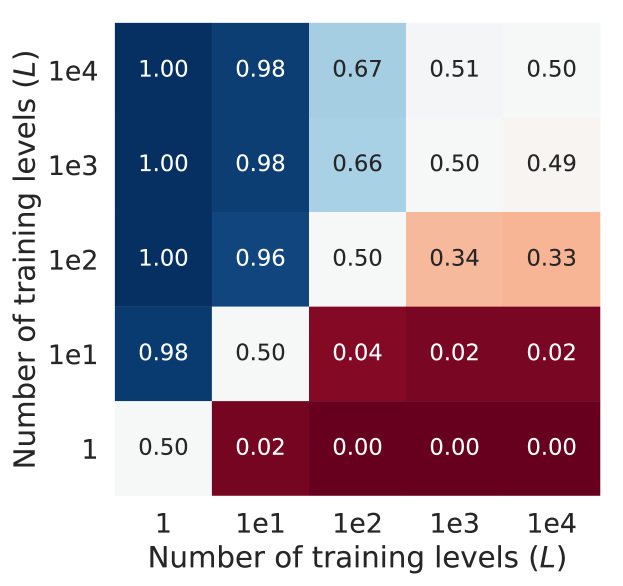
We also assess population performance through cross-play evaluation—that is, by evaluating agents in groups formed from two different training populations. We evaluate populations in cross-play both on the level(s) in their training set and on the held-out test levels. Specifically, for every pair of populations A and B, the training-level evaluation places agents sampled from population A (e.g., trained on level) with agents sampled from population B (e.g., trained on levels) in a level from the intersection of the populations’ training sets. The held-out evaluation similarly samples agents from populations A and B, but uses a level not found in either of the populations’ training sets.
As each environment requires a different number of players, we group agents from populations A and B as shown in Table 1. For HarvestPatch, Traffic Navigation, and Overcooked, we report the individual rewards achieved by the agents sampled from population A. For Capture the Flag, we analogously report the win rate for the agents from population A.
| Population: | ||
|---|---|---|
| Environment | A | B |
| HarvestPatch | 1 | 5 |
| Traffic Navigation | 1 | 7 |
| Overcooked | 1 | 1 |
| Capture the Flag | 2 | 2 |
4.2 Investigating Population Diversity
We run a second set of experiments to investigate how population diversity affects generalization. Measuring and optimizing for agent diversity are established challenges in reinforcement learning research. In single-agent domains, diversity is often estimated over behavioral trajectories or state-action distributions dai2022diversity ; haarnoja2017reinforcement . Prior multi-agent projects have largely focused on two-player zero-sum games balduzzi2019open ; nieves2021modelling . In these environments, the diversity of a set of agent strategies can be directly estimated from the empirical payoff matrix, rather than behavioral trajectories.
Given the varied environments used in our experiments (and particularly the cooperative and competitive natures of their payoff structures), we draw inspiration from the former approach, focusing on heterogeneity in agent behavior. This paper uses the term “population diversity” to refer to variation in the set of potential co-player policies that a new individual joining a population might face mckee2020social . High policy diversity maximizes coverage over the set of all possible behaviors in an environment (including potentially suboptimal or useless behaviors) eysenbach2018diversity , while low policy diversity consistently maps a given state to the same behavior, regardless of the agents involved.
In multi-agent research, the increasing prevalence of population play and population-based training make population size a commonly tuned feature of experimental design. Prior studies suggest that larger population sizes can increase policy diversity czarnecki2020real ; sanjaya2021measuring . We directly examine how varying population size affects diversity by training agents in populations of size for each environment. For Capture the Flag experiments, we additionally train populations with .
Expected Action Variation
Researchers should ideally be able to estimate population diversity in a task-agnostic manner, but in practice diversity is often evaluated using specific knowledge about the environment (e.g., unit composition in StarCraft II vinyals2019grandmaster ).
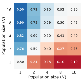
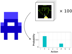
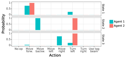
To address this challenge, we introduce a new method of measuring behavioral diversity in a population that we call expected action variation (EAV; Algorithm 1 in Appendix C.1). Intuitively, this metric captures the probability that two agents sampled at random from the population will select different actions when provided the same state (Figure 2). At a high level, we compute expected action variation by simulating a number of rollouts for each policy in the population and calculating the total variational distance between the resulting action distributions. One of the key advantages of this metric is that it can be naïvely applied to a set of stochastic policies generated in any environment.
Expected action variation ranges in value from to : a value of indicates that the population is behaviorally homogeneous (all agents select the same action for any given agent state), whereas a value of indicates that the population is maximally behaviorally diverse (all agents select different actions for any given agent state). An expected action variation of indicates that if two agents are sampled at random from the population and provided a representative state, they are just as likely to select the same action as they are to select different actions.
This procedure is designed to help compare diversity across populations and to reason about the way a focal agent’s experience of the game might change as a function of which co-players are encountered. Expected action variation is affected by stochasticity in policies, since such stochasticity can affect the state transitions that a focal agent experiences. Expected action variation is not intended to test whether the behavioral diversity of a population is significantly different from zero (or from ), since such a difference could emerge for trivial reasons.
We leverage expected action variation to assess the effect of population size on behavioral diversity. We also include additional baselines to help explore the dynamics of co-player diversity. Specifically, we train several populations parameterized with an intrinsic motivation module singh2005intrinsically on levels. In particular, we use the SVO component to motivate agents in these populations to maintain target distributions of reward mckee2020social . Each population is parameterized with either a homogeneous or heterogeneous distribution of SVO targets (see Appendix B.2.3).
Cross-Play Evaluation
We employ a cross-play evaluation procedure to measure the performance resulting from varying population sizes, following Section 4.1. Specifically, we group agents sampled from populations A and B and then evaluate group performance on a level from the intersection of the populations’ training sets. We use the same grouping and reporting procedure as before.
4.3 Quantifying Performance
For the majority of our environments, we quantify and analyze the individual rewards earned by the agents. In Capture the Flag, we evaluate agents in team competition. Consequently, we record the result of each match from which we calculate win rates and skill ratings. To estimate each population’s skill, we use the Elo rating system elo1978rating , an evaluation metric commonly used in games such as chess (see Appendix C.2 for details).
4.4 Statistical Analysis
In our experiments, we launch multiple independent training runs for each value of and each value of being investigated. Critically, we match the training sets of these independent runs across values of and . For example, the first run of the HarvestPatch experiment trains on the exact same training set as the first runs of the experiments. Similarly, the second runs for each of the to experiments use the same training set, and so on. This allows us to avoid confounding the effects of with those of and vice versa.
For our statistical analyses, we primarily leverage the Analysis of Variance (ANOVA) method fisher1928statistical . The ANOVA allows us to test whether changing the value of an independent variable (e.g., environment diversity) significantly affects the value of a specified dependent variable (e.g., individual reward). Each ANOVA is summarized with an -statistic and a -value. In cases where we repeat ANOVAs for each environment, we apply a Holm–Bonferroni correction to control the probability of false positives holm1979simple .
5 Results
5.1 Environment Diversity
To begin, we assess how environment diversity (i.e., the number of unique levels used for training) affects generalization. Agents are trained on levels in populations of size .
5.1.1 Generalization Gap Analysis
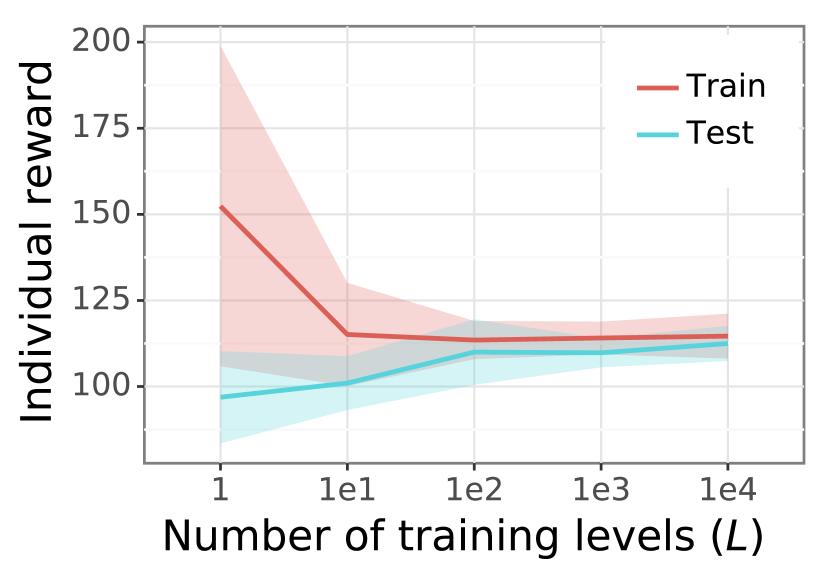
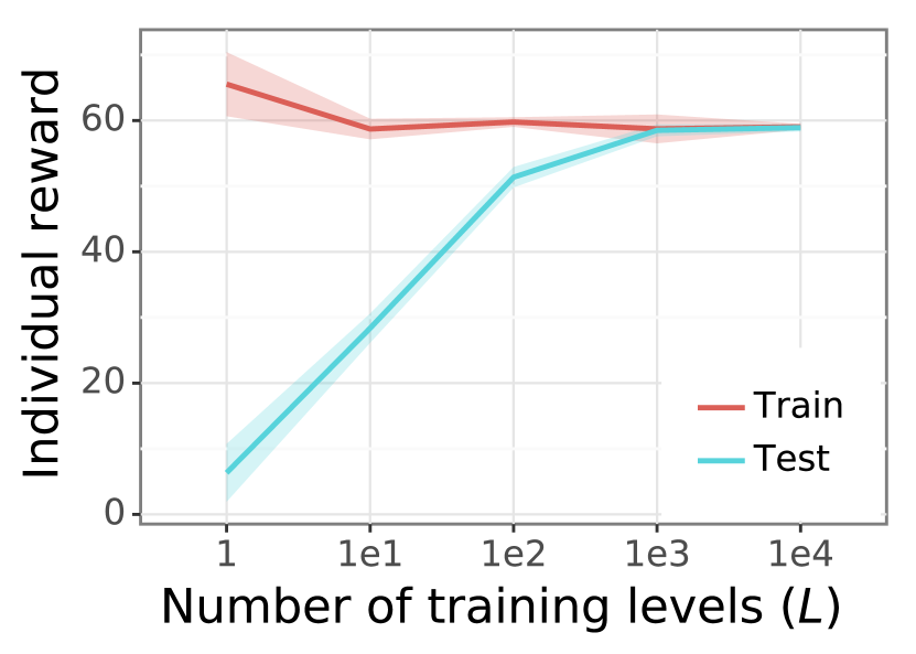
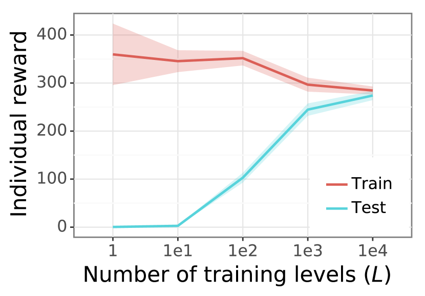
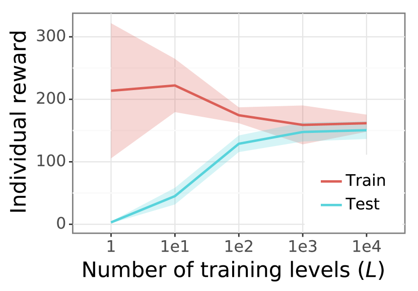
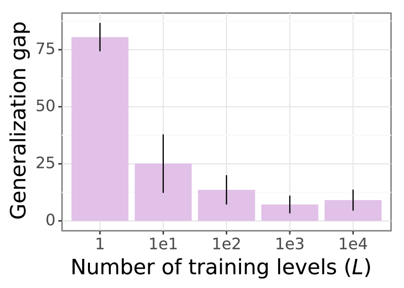
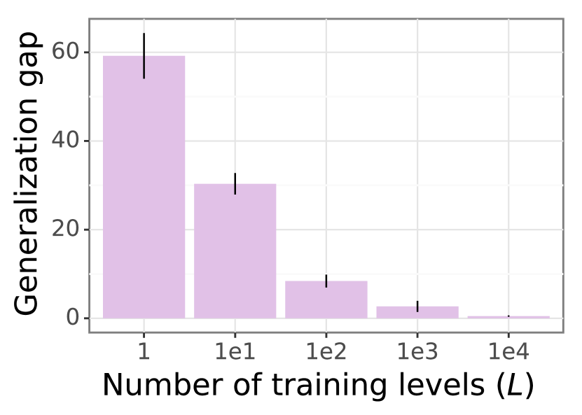
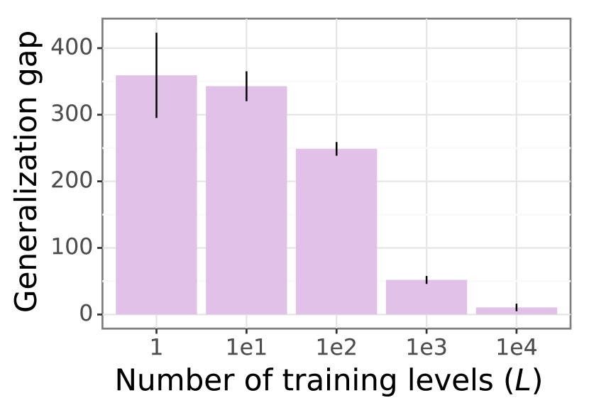
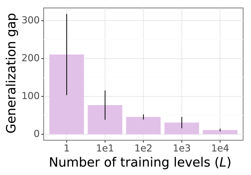
As shown in Figure 3, for all environments generalization improves as the number of levels used for training increases. Performance on the test set increases as increases, while performance on the training set tends to decrease with greater values of (Figure 3, top row).
Performance on the training set experiences a minor decrease from low to high values of . In contrast, the variance in training-set performance declines considerably as environment diversity increases. The variance in training-set performance is notably large for HarvestPatch and Capture the Flag when . This variability likely results from the wide distribution of possible rewards in the generated levels (e.g., due to varying apple density in HarvestPatch or map size in Capture the Flag). For Capture the Flag, the observed variance may also stem from the inherent difficulty of learning navigation behaviors on a singular large level where the rewards are sparse (i.e., without the availability of a natural curriculum).
To avoid ecological fallacy freedman1999ecological , we directly quantify and analyze the generalization gap with the procedure outlined in Section 4.1. As environment diversity increases, the generalization gap between the training and test sets decreases substantially (Figure 3, bottom row). The trend is sizeable, materializing even in the shift from to . Across the environments considered here, the generalization gap approaches zero around values of . A set of ANOVAs confirm that has a statistically significant effect on generalization in HarvestPatch, , , Traffic Navigation, , , Overcooked, , , and Capture the Flag, , (-values adjusted for multiple comparisons with a Holm–Bonferroni correction).
5.1.2 Cross-Play Evaluation
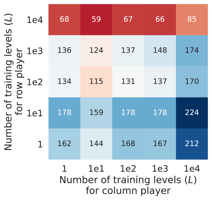
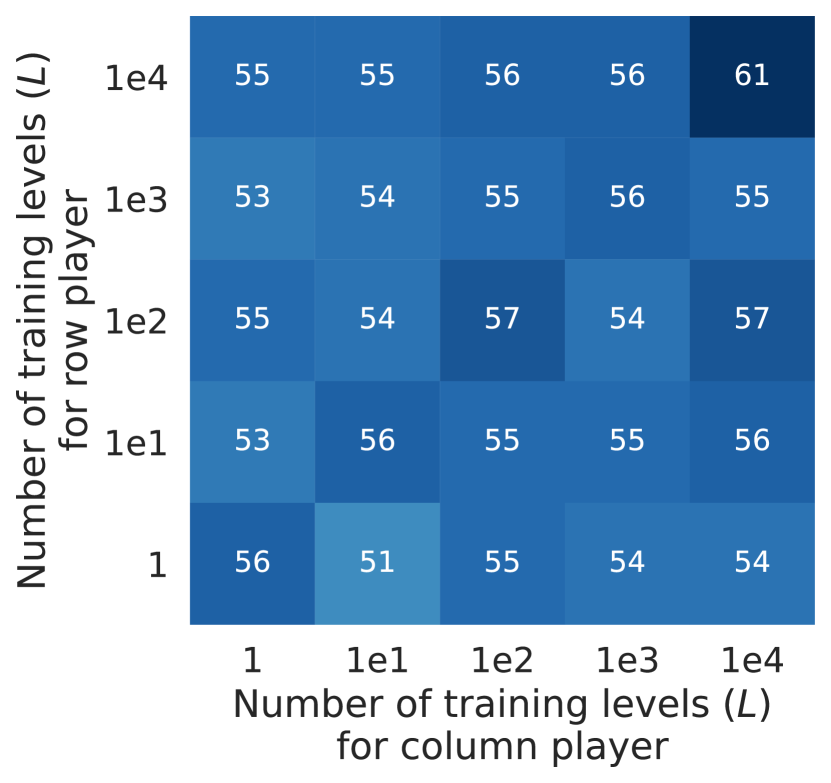
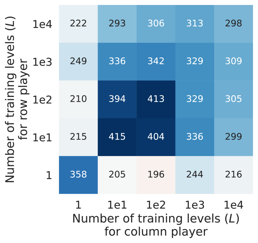
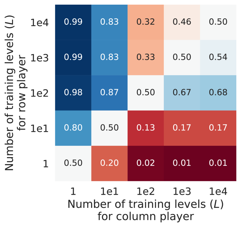
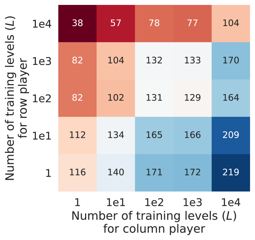
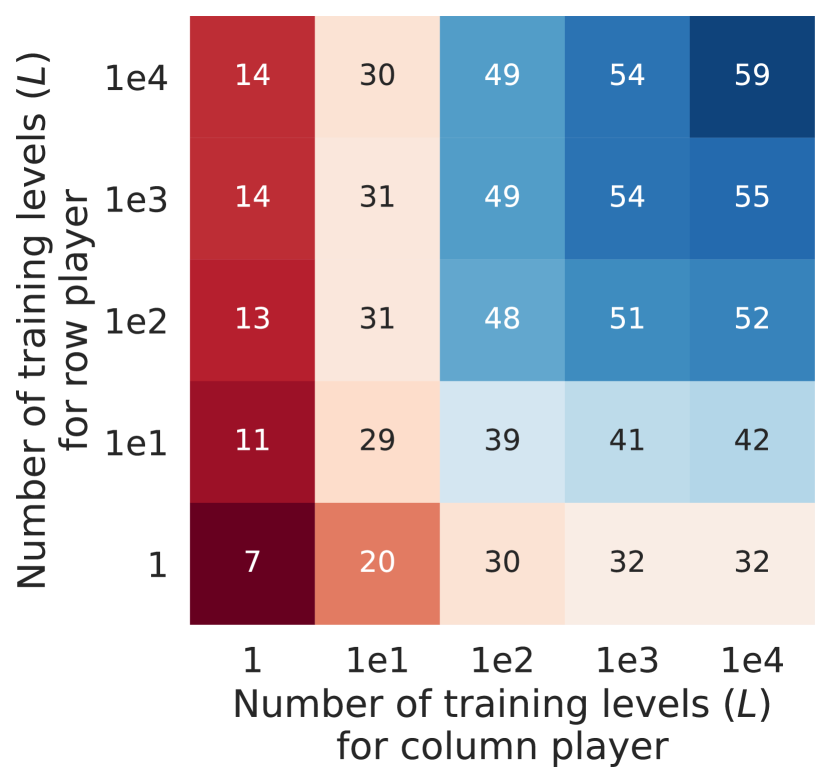
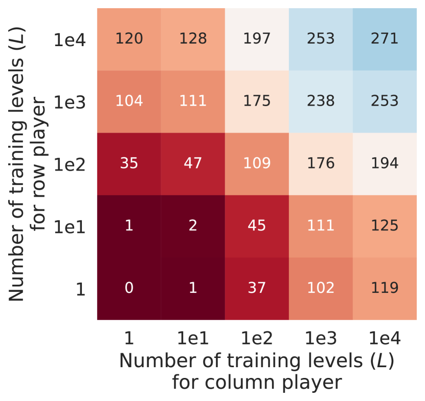
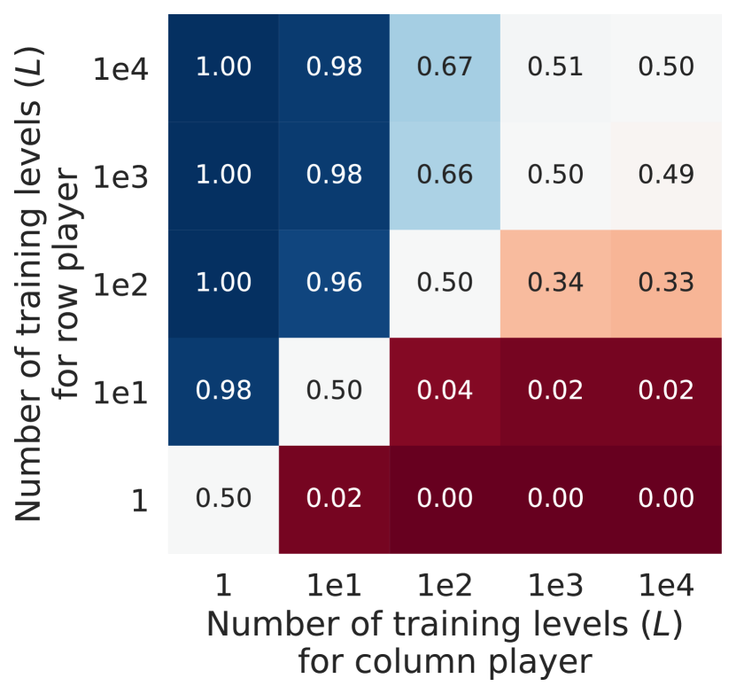
Next, we conduct cross-play evaluations of all populations following the procedure outlined in Section 4.1. We separately evaluate populations on the single level included in the training set for all populations (Figure 4, top row) and the held-out test levels (Figure 4, bottom row).
Overall, the effects of environment diversity vary substantially across environments.
HarvestPatch
We observe the highest level of performance for the agents playing with a group trained on a large number of levels (column ) after themselves training on a small number of levels (row ). In contrast, the worst-performing agents play with a group trained on a small number of levels (column ) after themselves training on a large number of levels (row ). These patterns emerge in both the training-level and test-level evaluations.
Traffic Navigation
Agents perform equally well on their training level across all values for their training set size and for the training set size of the group’s other members. In contrast, when evaluating agents on held-out test levels, an agent’s performance strongly depends on how many levels the agent and its group were trained on. Average rewards increase monotonically from column to column , and increase near-monotonically from row to row . Navigation appears more successful with increasing experience of various level layouts and with increasingly experienced groupmates.
Overcooked
In the held-out evaluations, we observe a consistent improvement in rewards earned from the bottom left ( grouped with ) to the top right ( grouped with ). An agent benefits both from playing with a partner with diverse training and from itself training with environment diversity.
A different pattern emerges in the training-level evaluation. Team performance generally decreases when one of the two agents trains on just levels. However, when both agents train on , they collaborate fairly effectively. The highest scores occur at the intermediate values and , rather than at . Population skill on training levels declines with increasing environment diversity.
Capture the Flag
Team performance is closely tied to environment diversity. A team’s odds of winning are quite low when they train on a smaller level set than the opposing team, and the win rate tends to jump considerably as soon as a team’s training set is larger than their opponents’. However, echoing the results in Overcooked, agents trained on an intermediate level-set size achieve the highest performance on training levels. Population skill actually decreases above on these levels (Table 2, middle column). In contrast, in held-out evaluation, environment diversity consistently strengthens performance; Elo ratings monotonically increase as increases (Table 2, right column).
| Elo rating on: | ||
|---|---|---|
| Training level | Test set | |
| 604 | 258 | |
| 882 | 773 | |
| 1245 | 1248 | |
| 1142 | 1349 | |
| 1124 | 1369 | |
5.2 Population Diversity
We next delve into the effects of population diversity on agent policies and performance. Agents are trained in populations of size on levels. In Capture the Flag, a set of additional populations are trained with size .
5.2.1 Expected Action Variation Analysis
We investigate the behavioral diversity of each population by calculating their expected action variation (see Section 4.2).
| Elo rating | |
|---|---|
| 751 | |
| 936 | |
| 1042 | |
| 1123 | |
| 1145 |
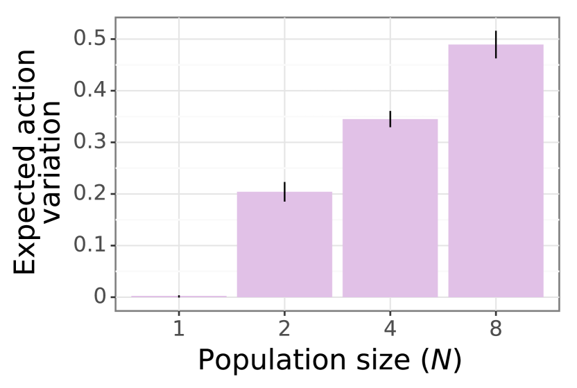
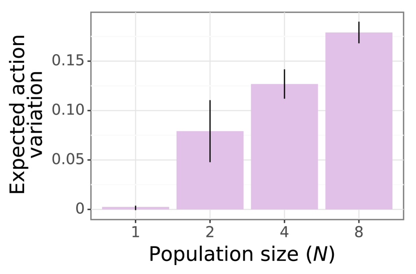
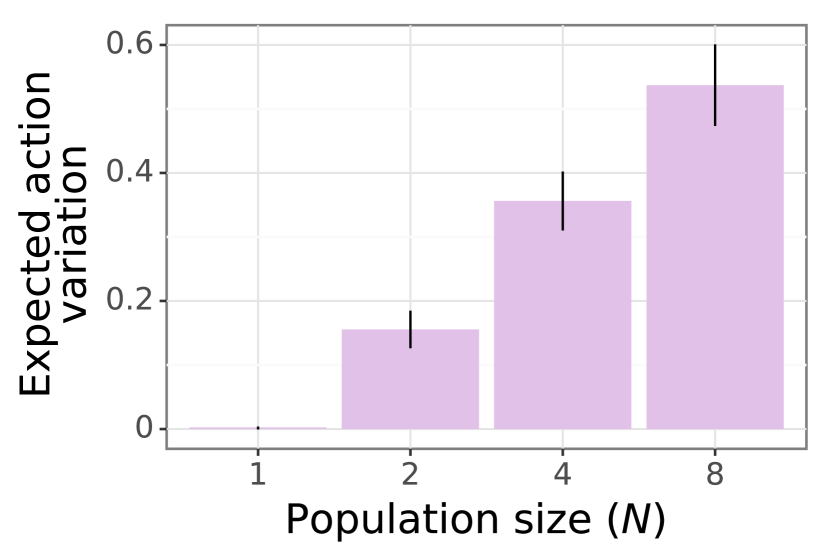
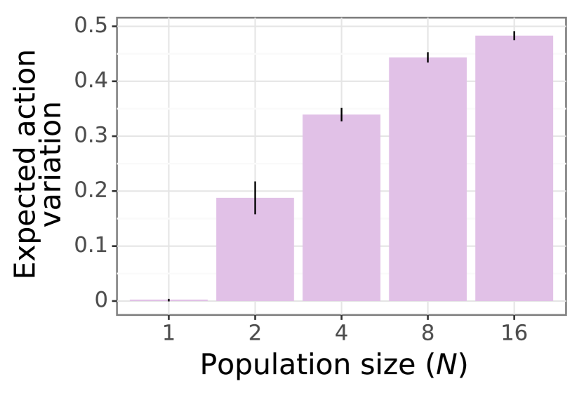
As shown in Figure 5, population size positively associates with behavioral diversity among agents trained in each environment. A set of ANOVAs confirm that has a statistically significant effect on expected action variation in HarvestPatch, , , Traffic Navigation, , , Overcooked, , , and Capture the Flag, , (-values adjusted for multiple comparisons with a Holm–Bonferroni correction). Increasing population size amplifies co-player diversity, without requiring any explicit optimization for variation. Multiple sources likely contribute to this diversity, including random initialization for agents and independent exploration and learning.
Intrinsic Motivation and Behavioral Diversity
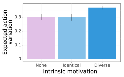
Prior studies demonstrate that parameterizing an agent population with heterogeneous levels of intrinsic motivation can induce behavioral diversity, as measured through task-specific, hard-coded metrics mckee2020social . These agent populations benefited from the resulting diversity in social dilemma tasks, including HarvestPatch. We run an experiment to confirm that this behavioral diversity can be detected through the measurement of expected action variation. Following prior work on HarvestPatch, we endow several populations with SVO, an intrinsic motivation for maintaining a target distribution of reward among group members, and then train them on levels. We parameterize these populations with either a homogeneous or heterogeneous distribution of SVO (see Appendix B.2.3 for details).
As seen in Figure 6, populations with heterogeneous intrinsic motivation exhibit significantly greater behavioral diversity than populations without intrinsic motivation, . In contrast, behavioral diversity does not differ significantly between populations of agents lacking intrinsic motivation and those parameterized with homogeneous intrinsic motivation, . These results help baseline the diversity induced by increasing population size and demonstrate that expected action variation can be used to assess established sources of behavioral heterogeneity.
5.2.2 Cross-Play Evaluation
We next conduct a cross-play evaluation of all populations following the procedure outlined in Section 4.2. As before, we test whether observed patterns are statistically significant using a set of ANOVAs (with a Holm–Bonferroni correction to account for multiple comparisons).
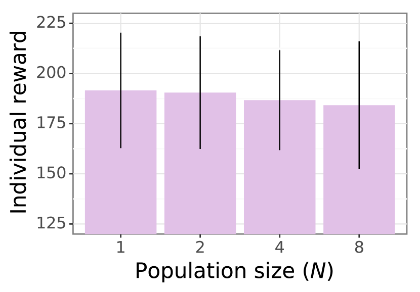
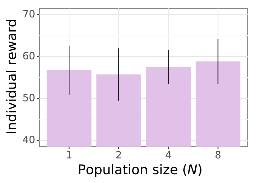
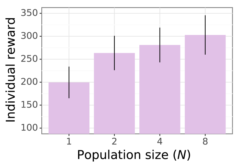
Population diversity does not significantly affect agent rewards for HarvestPatch, , (Figure 7a), and Traffic Navigation, , (Figure 7b). Agents trained through self-play () perform equivalently to agents from the largest, most diverse populations (). Training in a diverse population thus appears to neither advantage nor disadvantage agents in these environments.
In contrast, agents trained in diverse populations outperform those trained in lower-variation populations for Overcooked, , (Figure 7c) and Capture the Flag (Figure 7d). For both environments, we observe a substantial jump in performance from to and diminishing increases thereafter. The diminishing returns of diversity resemble the relationship between environment diversity and performance observed for Overcooked and Capture the Flag in Section 5.1.2.
6 Discussion
In summary, this paper makes several contributions to multi-agent reinforcement learning research. Our experiments extend single-agent findings on environment diversity and policy generalization to the multi-agent domain. We find that applying a small amount of environment diversity can lead to a substantial improvement in the generality of agents. However, this generalization reduces performance on agents’ training set for certain environments and co-players.
The expected action variation metric demonstrates how population size and the diversification of agent hyperparameters can influence behavioral diversity. As with environmental diversity, we find that training with a diverse set of co-players strengthens agent performance in some (but not all) cases.
Expected action variation measures population diversity by estimating the heterogeneity in a population’s policy distribution. As recognized by hierarchical and options-based frameworks sutton1999between , the mapping of lower-level actions to higher-level strategic outcomes is imperfect; in some states, different actions may lead to identical outcomes. Higher levels of expected action variation may capture greater strategic diversity. Nonetheless, future work could aim to directly measure variation in a population’s strategy set.
These findings may prove useful for the expanding field of human-agent cooperation research. Human behavior is notoriously variable cronbach1957two ; eid1999intraindividual . Interindividual differences in behavior can be a major difficulty for agents intended to interact with humans egan1988individual . This variance thus presents a major challenge stymying the development of human-compatible reinforcement learning agents. Improving the generalizability of our agents could advance progress toward human compatibility, especially for cooperative domains dafoe2020open .
Future work could seek to develop more sophisticated approaches for quantifying diversity. For example, here we use the “number of unique levels” metric as a proxy of environment diversity, and therefore increased leads to monotonically increasing environment diversity. However, these levels may be unique in ways which are irrelevant to the agents. Scaling existing approaches to these settings, such as those that study how the environment influences agent behaviour wang2020enhanced , may help determine which features correspond to meaningful diversity.
The experiments presented here employ a rigorous statistical approach to test the consistency and significance of the effects in question. Consequently, they help scope the benefits of environment and population diversity for multi-agent reinforcement learning. Overall, we hope that these findings can improve the design of future multi-agent studies, leading to more generalized agents.
Acknowledgements
We thank Ian Gemp, Edgar Duéñez-Guzmán, and Thore Graepel for their support and feedback during the preparation of this manuscript. We are also indebted to Mary Cassin for designing and creating the sprite art for the DeepMind Lab2D implementation of Overcooked.
References
- (1) Balduzzi, D., Garnelo, M., Bachrach, Y., Czarnecki, W., Perolat, J., Jaderberg, M., Graepel, T.: Open-ended learning in symmetric zero-sum games. In: International Conference on Machine Learning, pp. 434–443. PMLR (2019)
- (2) Beattie, C., Köppe, T., Duéñez-Guzmán, E.A., Leibo, J.Z.: DeepMind Lab2D. arXiv preprint arXiv:2011.07027 (2020)
- (3) Carroll, M., Shah, R., Ho, M.K., Griffiths, T., Seshia, S., Abbeel, P., Dragan, A.: On the utility of learning about humans for human-AI coordination. In: Advances in Neural Information Processing Systems, pp. 5175–5186 (2019)
- (4) Charakorn, R., Manoonpong, P., Dilokthanakul, N.: Investigating partner diversification methods in cooperative multi-agent deep reinforcement learning. In: International Conference on Neural Information Processing, pp. 395–402. Springer (2020)
- (5) Cobbe, K., Hesse, C., Hilton, J., Schulman, J.: Leveraging procedural generation to benchmark reinforcement learning. arXiv preprint arXiv:1912.01588 (2019)
- (6) Cobbe, K., Klimov, O., Hesse, C., Kim, T., Schulman, J.: Quantifying generalization in reinforcement learning. In: International Conference on Machine Learning, pp. 1282–1289 (2019)
- (7) Cronbach, L.J.: The two disciplines of scientific psychology. American Psychologist 12(11), 671 (1957)
- (8) Czarnecki, W.M., Gidel, G., Tracey, B., Tuyls, K., Omidshafiei, S., Balduzzi, D., Jaderberg, M.: Real world games look like spinning tops. Advances in Neural Information Processing Systems 33, 17443–17454 (2020)
- (9) Dafoe, A., Hughes, E., Bachrach, Y., Collins, T., McKee, K.R., Leibo, J.Z., Larson, K., Graepel, T.: Open problems in cooperative AI. arXiv preprint arXiv:2012.08630 (2020)
- (10) Dai, T., Du, Y., Fang, M., Bharath, A.A.: Diversity-augmented intrinsic motivation for deep reinforcement learning. Neurocomputing 468, 396–406 (2022)
- (11) Egan, D.E.: Individual differences in human-computer interaction. In: Handbook of Human-Computer Interaction, pp. 543–568. Elsevier (1988)
- (12) Eid, M., Diener, E.: Intraindividual variability in affect: Reliability, validity, and personality correlates. Journal of Personality and Social Psychology 76(4), 662 (1999)
- (13) Elo, A.E.: The Rating of Chessplayers, Past and Present. Arco Publishing (1978)
- (14) Everett, R., Cobb, A., Markham, A., Roberts, S.: Optimising worlds to evaluate and influence reinforcement learning agents. In: Proceedings of the 18th International Conference on Autonomous Agents and Multiagent Systems, pp. 1943–1945. International Foundation for Autonomous Agents and Multiagent Systems (2019)
- (15) Eysenbach, B., Gupta, A., Ibarz, J., Levine, S.: Diversity is all you need: Learning skills without a reward function. In: International Conference on Learning Representations (2019)
- (16) Fisher, R.A.: Statistical Methods for Research Workers. Oliver & Boyd (1928)
- (17) Freedman, D.A.: Ecological inference and the ecological fallacy. International Encyclopedia of the Social & Behavioral Sciences 6(4027-4030), 1–7 (1999)
- (18) Haarnoja, T., Tang, H., Abbeel, P., Levine, S.: Reinforcement learning with deep energy-based policies. In: International Conference on Machine Learning, pp. 1352–1361. PMLR (2017)
- (19) Hessel, M., Soyer, H., Espeholt, L., Czarnecki, W., Schmitt, S., van Hasselt, H.: Multi-task deep reinforcement learning with PopArt. In: Proceedings of the AAAI Conference on Artificial Intelligence, vol. 33, pp. 3796–3803 (2019)
- (20) Holm, S.: A simple sequentially rejective multiple test procedure. Scandinavian Journal of Statistics pp. 65–70 (1979)
- (21) Hu, H., Lerer, A., Peysakhovich, A., Foerster, J.: ‘Other-play’ for zero-shot coordination. arXiv preprint arXiv:2003.02979 (2020)
- (22) Hughes, E., Leibo, J.Z., Phillips, M., Tuyls, K., Dueñez-Guzman, E., Castañeda, A.G., Dunning, I., Zhu, T., McKee, K.R., Koster, R., Roff, H., Graepel, T.: Inequity aversion improves cooperation in intertemporal social dilemmas. In: Advances in Neural Information Processing Systems, pp. 3326–3336 (2018)
- (23) Ibrahim, A., Jitani, A., Piracha, D., Precup, D.: Reward redistribution mechanisms in multi-agent reinforcement learning. In: Adaptive Learning Agents Workshop at the International Conference on Autonomous Agents and Multiagent Systems (2020)
- (24) Jaderberg, M., Czarnecki, W.M., Dunning, I., Marris, L., Lever, G., Castañeda, A.G., Beattie, C., Rabinowitz, N.C., Morcos, A.S., Ruderman, A., Sonnerat, N., Green, T., Deason, L., Leibo, J.Z., Silver, D., Hassabis, D., Kavukcuoglu, K., Graepel, T.: Human-level performance in 3D multiplayer games with population-based reinforcement learning. Science 364(6443), 859–865 (2019)
- (25) Jaques, N., Lazaridou, A., Hughes, E., Gulcehre, C., Ortega, P.A., Strouse, D., Leibo, J.Z., De Freitas, N.: Intrinsic social motivation via causal influence in multi-agent RL. In: International Conference on Learning Representations (2019)
- (26) Juliani, A., Khalifa, A., Berges, V.P., Harper, J., Teng, E., Henry, H., Crespi, A., Togelius, J., Lange, D.: Obstacle tower: A generalization challenge in vision, control, and planning. arXiv preprint arXiv:1902.01378 (2019)
- (27) Justesen, N., Torrado, R.R., Bontrager, P., Khalifa, A., Togelius, J., Risi, S.: Illuminating generalization in deep reinforcement learning through procedural level generation. arXiv preprint arXiv:1806.10729 (2018)
- (28) Kingma, D.P., Ba, J.: Adam: A method for stochastic optimization. arXiv preprint arXiv:1412.6980 (2014)
- (29) Knott, P., Carroll, M., Devlin, S., Ciosek, K., Hofmann, K., Dragan, A., Shah, R.: Evaluating the robustness of collaborative agents. arXiv preprint arXiv:2101.05507 (2021)
- (30) Kramár, J., Rabinowitz, N., Eccles, T., Tacchetti, A.: Should I tear down this wall? Optimizing social metrics by evaluating novel actions. arXiv preprint arXiv:2004.07625 (2020)
- (31) Lanctot, M., Zambaldi, V., Gruslys, A., Lazaridou, A., Tuyls, K., Pérolat, J., Silver, D., Graepel, T.: A unified game-theoretic approach to multiagent reinforcement learning. In: Advances in Neural Information Processing Systems, pp. 4190–4203 (2017)
- (32) Leibo, J.Z., Perolat, J., Hughes, E., Wheelwright, S., Marblestone, A.H., Duéñez-Guzmán, E., Sunehag, P., Dunning, I., Graepel, T.: Malthusian reinforcement learning. In: Proceedings of the 18th International Conference on Autonomous Agents and Multiagent Systems, pp. 1099–1107. International Foundation for Autonomous Agents and Multiagent Systems (2019)
- (33) Lerer, A., Peysakhovich, A.: Learning existing social conventions via observationally augmented self-play. In: Proceedings of the 2019 AAAI/ACM Conference on AI, Ethics, and Society, pp. 107–114 (2019)
- (34) Littman, M.L.: Markov games as a framework for multi-agent reinforcement learning. In: Machine Learning Proceedings 1994, pp. 157–163. Elsevier (1994)
- (35) Lowe, R., Wu, Y., Tamar, A., Harb, J., Abbeel, P., Mordatch, I.: Multi-agent actor-critic for mixed cooperative-competitive environments. In: Advances in Neural Information Processing Systems, pp. 6382–6393 (2017)
- (36) McKee, K.R., Gemp, I., McWilliams, B., Duéñez-Guzmán, E.A., Hughes, E., Leibo, J.Z.: Social diversity and social preferences in mixed-motive reinforcement learning. In: Proceedings of the 19th International Conference on Autonomous Agents and Multiagent Systems. International Foundation for Autonomous Agents and Multiagent Systems (2020)
- (37) Nieves, N.P., Yang, Y., Slumbers, O., Mguni, D.H., Wen, Y., Wang, J.: Modelling behavioural diversity for learning in open-ended games. arXiv preprint arXiv:2103.07927 (2021)
- (38) Perolat, J., Leibo, J.Z., Zambaldi, V., Beattie, C., Tuyls, K., Graepel, T.: A multi-agent reinforcement learning model of common-pool resource appropriation. In: Advances in Neural Information Processing Systems, pp. 3643–3652 (2017)
- (39) Sanjaya, R., Wang, J., Yang, Y.: Measuring the non-transitivity in chess. arXiv preprint arXiv:2110.11737 (2021)
- (40) Singh, S.P., Barto, A.G., Chentanez, N.: Intrinsically motivated reinforcement learning. In: Advances in Neural Information Processing Systems (2005)
- (41) Song, H.F., Abdolmaleki, A., Springenberg, J.T., Clark, A., Soyer, H., Rae, J.W., Noury, S., Ahuja, A., Liu, S., Tirumala, D., Heess, N., Belov, D., Riedmiller, M., Botvinick, M.M.: V-MPO: On-policy maximum a posteriori policy optimization for discrete and continuous control. arXiv preprint arXiv:1909.12238 (2019)
- (42) Sutton, R.S., Precup, D., Singh, S.: Between MDPs and semi-MDPs: A framework for temporal abstraction in reinforcement learning. Artificial Intelligence 112(1-2), 181–211 (1999)
- (43) Tukey, J.W.: Comparing individual means in the analysis of variance. Biometrics pp. 99–114 (1949)
- (44) Vinyals, O., Babuschkin, I., Czarnecki, W.M., Mathieu, M., Dudzik, A., Chung, J., Choi, D.H., Powell, R., Ewalds, T., Georgiev, P., Oh, J., Horgan, D., Kroiss, M., Danihelka, I., Huang, A., Sifre, L., Cai, T., Agapiou, J.P., Jaderberg, M., Vezhnevets, A.S., Leblond, R., Pohlen, T., Dalibard, V., Budden, D., Sulsky, Y., Molloy, J., Paine, T.L., Gulcehre, C., Wang, Z., Pfaff, T., Wu, Y., Ring, R., Yogatama, D., Wünsch, D., McKinney, K., Smith, O., Schaul, T., Lillicrap, T., Kavukcuoglu, K., Hassabis, D., Apps, C., Silver, D.: Grandmaster level in StarCraft II using multi-agent reinforcement learning. Nature 575(7782), 350–354 (2019)
- (45) Wang, R., Lehman, J., Clune, J., Stanley, K.O.: Paired open-ended trailblazer (POET): Endlessly generating increasingly complex and diverse learning environments and their solutions. arXiv preprint arXiv:1901.01753 (2019)
- (46) Wang, R., Lehman, J., Rawal, A., Zhi, J., Li, Y., Clune, J., Stanley, K.: Enhanced POET: Open-ended reinforcement learning through unbounded invention of learning challenges and their solutions. In: International Conference on Machine Learning, pp. 9940–9951. PMLR (2020)
- (47) Wang, R.E., Wu, S.A., Evans, J.A., Tenenbaum, J.B., Parkes, D.C., Kleiman-Weiner, M.: Too many cooks: Bayesian inference for coordinating multi-agent collaboration. Cooperative AI Workshop at the Conference on Neural Information Processing Systems (2020)
- (48) Zhang, C., Vinyals, O., Munos, R., Bengio, S.: A study on overfitting in deep reinforcement learning. arXiv preprint arXiv:1804.06893 (2018)
Appendix A Environments
A.1 HarvestPatch
A.1.1 Gameplay
Players are placed in a gridworld environment containing a number of apples. Players can harvest apples by moving over them, receiving reward for each apple collected. Apples regrow after being harvested. The rate of apple regrowth is determined by the number of unharvested apples within the regrowth radius . An apple cannot regrow if there are no apples within its radius or if a player is standing on its cell. This property induces a social dilemma for the players. The group as a whole will perform better if its members are abstentious in their apple consumption, but in the short term individuals can always do better by harvesting greedily.
In addition to basic movement actions, players can use a beam to tag out other players. Players are tagged out for 50 steps after being struck by another group member’s tagging beam, and then are respawned at a random location within the environment. The ability to tag other players can be used to reduce the effective group size and mitigate the intensity of the social dilemma perolat2017multi . There are no direct reward penalties for tagging or being tagged; any reward penalties experienced by the agents are indirectly imposed through opportunity costs.
Observations
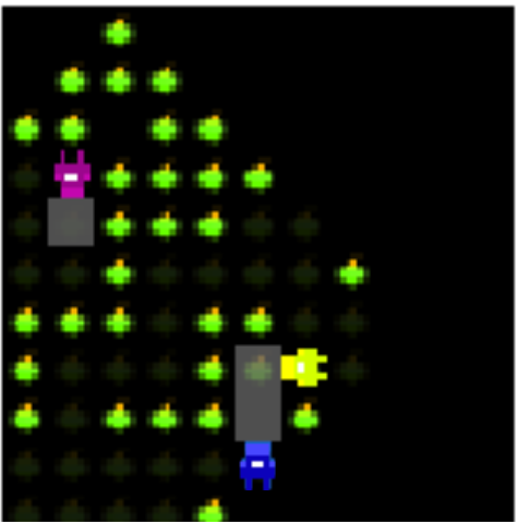
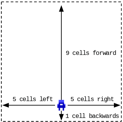
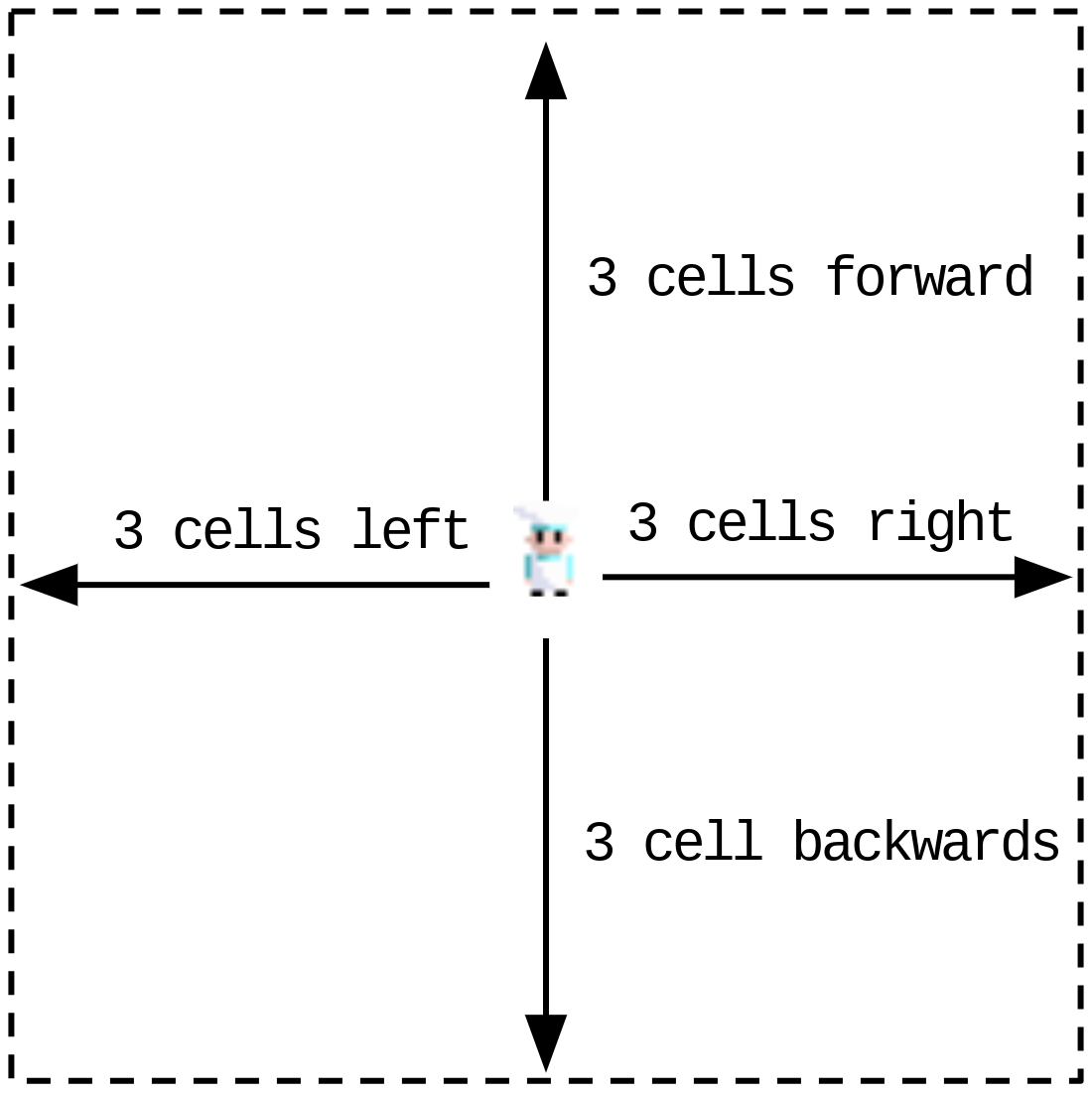
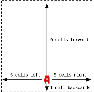
Players observe an egocentric view of the environment (Figure A1).
Actions
Players can take one of the following eight actions each step:
-
1.
No-op: The player stays in the same position.
-
2.
Move forward: Moves the player forwards one cell.
-
3.
Move backward: Moves the player backwards one cell.
-
4.
Move left: Moves the player left one cell.
-
5.
Move right: Moves the player right one cell.
-
6.
Turn left: Rotates the player 90 degrees anti-clockwise.
-
7.
Turn right: Rotates the player 90 degrees clockwise.
-
8.
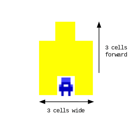
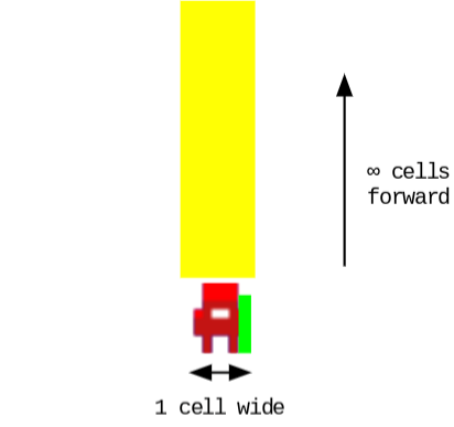
Use tag beam: Fires a short yellow beam forwards from the player. The beam is three cells wide and is projected three cells forwards.
The use tag beam action has a cooldown of four steps for each player. If the player tries to use the tag action during this cooldown period, the outcome is equivalent to the no-op action. Players who are hit by the beam are tagged out for 50 steps, after which they are respawned in a random location.
Rewards
Players receive reward for each apple they harvest. (Players can harvest an edible apple by moving into its cell.) Players do not receive reward in any other way. Notably, neither using the use tag beam action nor being hit by the tagging beam yields any reward.
Apple regrowth probabilities
In HarvestPatch, apples grow in “patches”. Each apple in a patch is within distance of the other apples in the patch, and further than away from apples in all other patches. Based on the respawn rule described previously, on each step of an episode, harvested apples have a probability of regrowing based on the number of other non-harvested apples in their patch. These probabilities are as follows:
| Number of | Regrowth |
|---|---|
| apples in patch | probability |
Crucially, when the patch has been depleted (i.e., the number of apples in patch is zero), the apples in that patch cannot regrow for the rest of the episode.
A.1.2 Additional details
The HarvestPatch environment instantiates an intertemporal social dilemma hughes2018inequity . A group can sustainably harvest from the environment by abstaining from fully depleting the apple patches. This strategy supplies the group with an indefinite stream of reward over time. However, for the group to reap the benefits of a sustainable harvesting strategy, every group member must abstain from depleting apple patches. In contrast, an individual is immediately and unilaterally guaranteed reward for eating an “endangered apple” (the last unharvested apple remaining in a given patch) if it acts greedily. Overall, there is a strong tension between the short-term individual temptation to maximize reward through unsustainable behavior and the long-term strategy of maximizing group welfare by acting sustainably.
A.1.3 Procedural generation
Procedure
To generate levels for HarvestPatch, we use the following procedure given a number of patches with a patch radius and density :
-
1.
Generate a area.
-
2.
Place points randomly, ensuring a distance of at least between all points.
-
3.
Around each point, assign apples in radius with probability per apple.
-
4.
Place player spawn points in random non-assigned cells.
Distribution over environmental features
Figure A2 presents the distribution of apple counts in HarvestPatch levels, alongside visualizations of the levels at the minimum, median, and maximum of this distribution. Similarly, Figure A3 presents an example level for each of the various values of the patch radius parameter .


Example levels
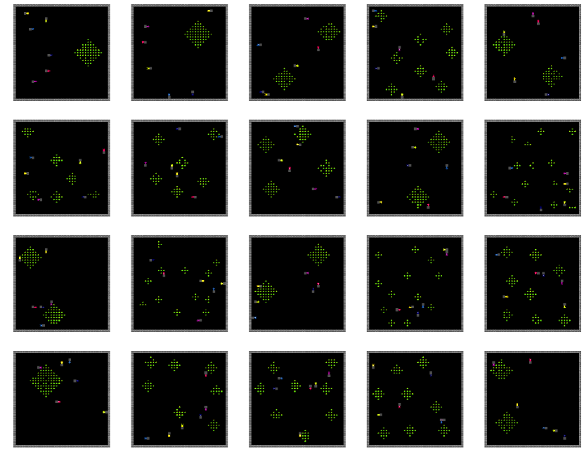
Presented in Figure A4 are 20 randomly sampled levels created through the previously described generation procedure.
A.2 Traffic Navigation
A.2.1 Gameplay
Eight players are placed along the edges of a gridworld environment. The goal for each player is to navigate through the level to their given “goal location” while avoiding collisions with other players. Goal locations are randomly sampled from the available edge cells in the game. More than one player can have the same goal at any one time. Upon a player reaching their given goal, they receive reward and are assigned a new goal location.
Levels created by the procedural generator can contain large open-spaces (making navigation and coordination easy), as well as small corridors (requiring additional coordination to avoid collisions with other players). While the number of players remains fixed (at eight), the size of the levels ranges from (100 cells in total) to (400 cells in total). For the smaller levels, while a players may chart a short path to their goal, the tight proximity of other players increases the likelihood of colliding into another player. In large levels, the goals are further apart, on expectation necessitating further travel for players to receive their reward. However, due to the larger size of the environment, the likelihood of players encountering one another is reduced.
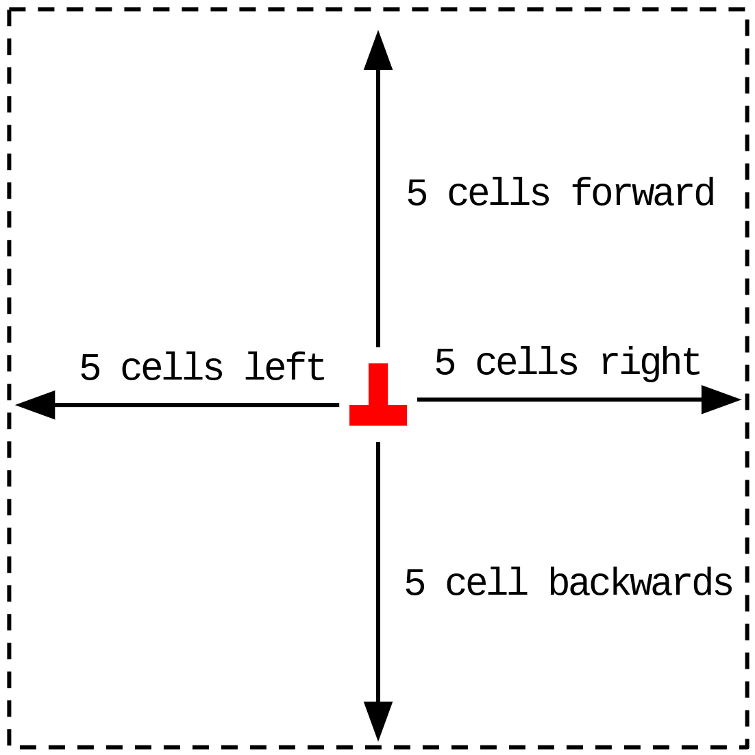
Observations
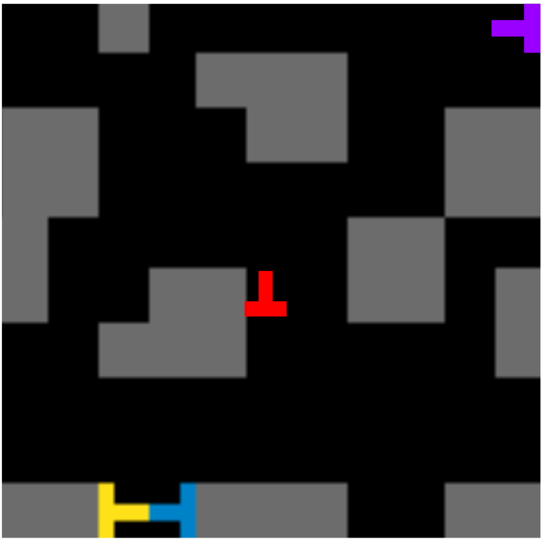
Players observe an egocentric view of the environment (Figure A5) as well as their relative offset to the current goal location.
Actions
Players can take one of the following five actions on each step:
-
1.
No-op: The player stays in the same position.
-
2.
Move north: Moves the player north one cell.
-
3.
Move south: Moves the player south one cell.
-
4.
Move west: Moves the player west one cell.
-
5.
Move east: Moves the player east one cell.
Rewards
Players receive reward when they successfully occupy the same cell as their goal location. They receive reward whenever they collide into another player (regardless of whether they or the other player caused the collision).
A.2.2 Procedural generation
Procedure
To generate levels for Traffic Navigation, we use the following procedure:
-
1.
Generate an area with a width and height .
-
2.
Add walls along the outer edge of this area.
-
3.
Remove two neighbouring walls for every player, adding a player spawn point at each newly available cell and adding those cells as available goal locations.
-
4.
Create a random number of wall blocks in the available area, ensuring that a majority of the blocks are more than two cells away from each other.
-
5.
Randomly scatter a number of individual walls within the available area.
-
6.
Check that the level is solvable: all goals are reachable from all starting locations.
Distribution over environmental features
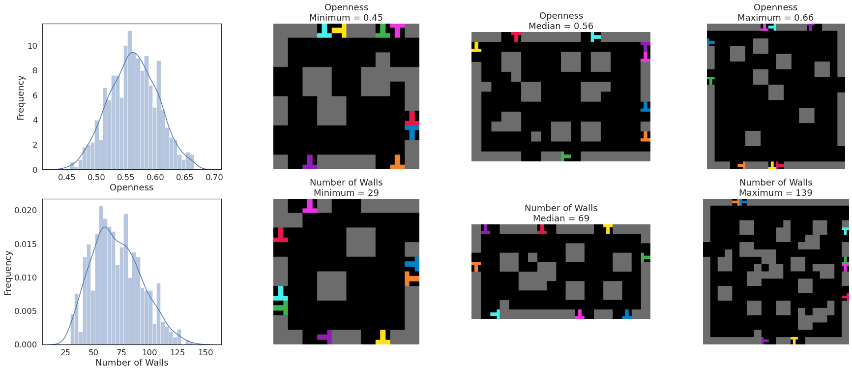
To demonstrate the diversity of the procedurally generated levels for Traffic Navigation, this section introduces four descriptive features, presents their distributions from 100,000 samples, and visualizes the minimum, medium, and maximum level of each distribution.
The two features are as follows:
-
1.
Openness: The proportion of non-wall cells in the level.
-
2.
Number of Walls: The number of walls in the level.
Example levels
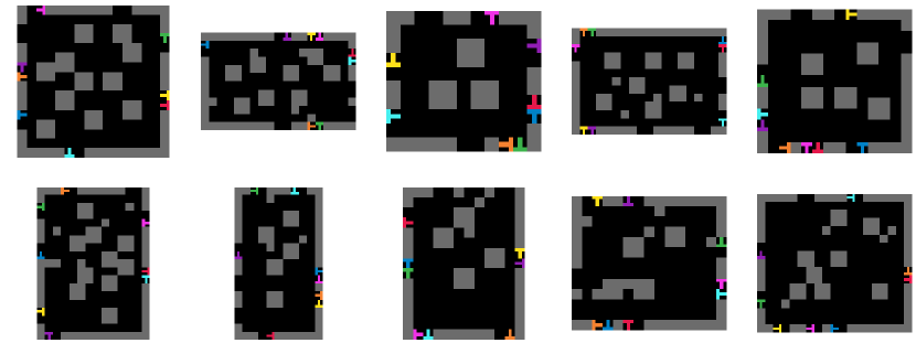
Presented in Figure A7 are 10 randomly sampled levels created through the previously described generation procedure.
A.3 Overcooked
A.3.1 Gameplay
Players are placed in a gridworld environment containing cooking pots, dispensing stations (tomatoes or dishes), delivery stations, and empty counters. Players can move around and interact with these objects. By sequencing certain object interactions, players can pick up and deposit items. Each player (and each counter) can only hold one item at a time.
The objective of each episode is for the players to deliver as many tomato soup dishes as possible through delivery stations. In order to create a tomato soup dish, players must pickup tomatoes and deposit them into the cooking pot. Once there are three tomatoes in the cooking pot, it begins to cook for 20 steps. After 20 steps, the soup is fully cooked. Cooking progress for a dish is tracked by a loading bar overlaying the cooking pot. The loading bar increments over the cooking time and then turns green when the dish is ready for collection.
When the tomato soup is ready for collection, a player holding an empty dish can interact with the cooking pot to pick up the soup. The player can then deliver the soup by interacting with a delivery station while holding the completed dish. A successful delivery rewards both players and removes the dish from the game.
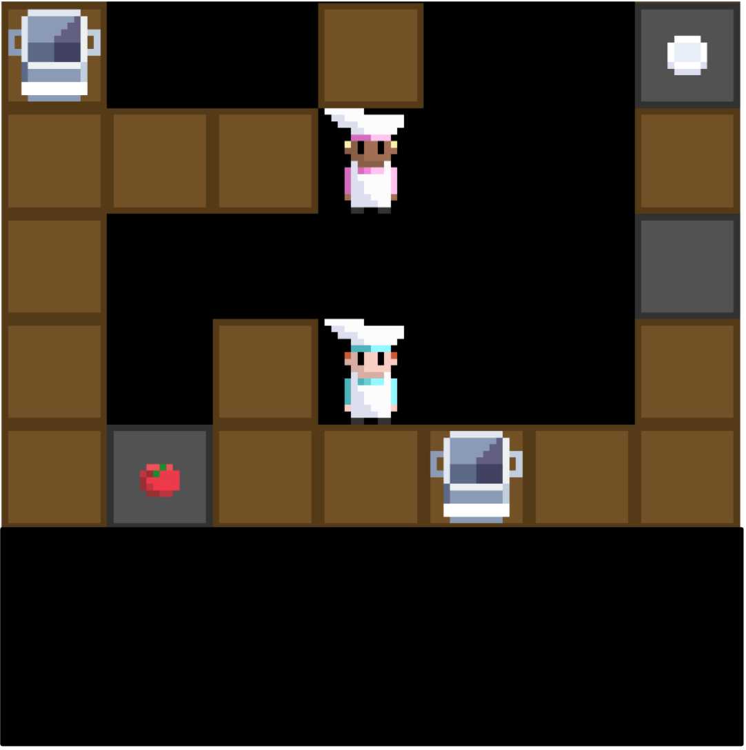
Observations
Players observe an egocentric view of the environment (Figure A8).
Actions
Players can take one of the following six actions each step:
-
1.
No-op: The player stays in the same position.
-
2.
Move north: Orients and moves the player north one cell.
-
3.
Move south: Orients and moves the player south one cell.
-
4.
Move west: Orients and moves the player west one cell.
-
5.
Move east: Orients and moves the player east one cell.
-
6.
Interact: The player interacts with the cell that they are facing.
The outcome of the Interact action depends on the current item held by the player (none, empty dish, tomato, or soup), as well as the type of object which they are facing (counter, cooking pot, tomato station, dish station, or delivery station). Depending on these two conditions, the player will either deposit the held item to the object or pick up an item from the object.
Rewards
Players receive a shared reward for every soup they deliver through the delivery station. As a result, they are incentivized to create and deliver as many soups as possible within an episode. To scaffold learning, players also receive reward each time they deposit a tomato into the cooking pot.
A.3.2 Procedural generation
Procedure
To generate levels for Overcooked, we use the following procedure:
-
1.
Generate an area with a width and height .
-
2.
Add counters along the outer edge of this area.
-
3.
Create a random number of counters within the available area, either as a block of counters in the middle or randomly scattered throughout the area.
-
4.
For each object in {cooking pot, tomato station, dish station, delivery station}, convert one to three counters into that object.
-
5.
Place two player spawn points in random non-assigned cells.
-
6.
Check that the level is solvable: tomato soups can be created and delivered by both players.
Distribution over environmental features
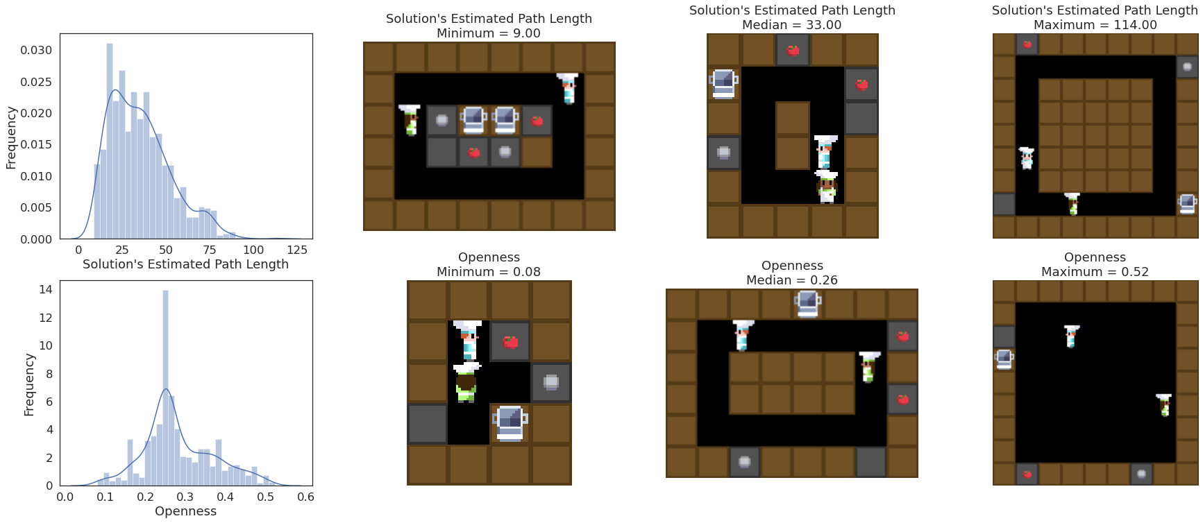
To demonstrate the diversity of the procedurally generated levels for Overcooked, this section introduces two descriptive features, presents their distributions from 100,000 samples, and visualizes the minimum, medium, and maximum level of each distribution.
The two features are as follows:
-
1.
Solution’s Estimated Path Length: The estimated number of required movement actions between the kitchen objects to create and delivery one tomato soup.
-
2.
Openness: The proportion of non-counter cells in the level.
Example levels
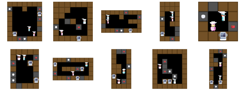
Presented in Figure A10 are 10 randomly sampled levels created through the previously described generation procedure.
A.4 Capture the Flag
A.4.1 Gameplay
Capture the Flag is played in a gridworld environment segmented by impassable walls and containing two bases. Players are divided into two teams and tasked with capturing the opposing team’s flag while simultaneously defending their own flag. Flags spawn within team bases. Players can capture the opposing team’s flag by first moving onto it (picking it up) and then returning it to their own base, while their own flag is there. Players observe an egocentric window around themselves. On each step, a player can move around the environment and fire a tag-out beam in the direction they are facing.
At the beginning of an episode, players start with three units of health. A player’s health is reduced by one each time it is tagged by a member of the opposing team. Upon reaching zero health, the player is tagged out for 20 steps. After 20 steps, the tagged-out player respawns at their base with three health. Players are rewarded for flag captures and returns, as well as for tagging opposing players.
Observations
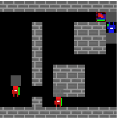
Players observe an egocentric view of the environment (see Figure A11), as well as a boolean value for each flag indicating whether it is being held by the opposing team.
Actions
Players can take one of the following eight actions each step:
-
1.
No-op: The player stays in the same position.
-
2.
Move forward: Moves the player forwards one cell.
-
3.
Move backward: Moves the player backwards one cell.
-
4.
Move left: Moves the player left one cell.
-
5.
Move right: Moves the player right one cell.
-
6.
Turn left: Rotates the player 90 degrees anti-clockwise.
-
7.
Turn right: Rotates the player 90 degrees clockwise.
-
8.
Use tag beam: Fires a yellow beam forwards from the player until it hits either a wall or another player.
The use tag beam action has a cooldown of three steps for each player. If the player tries to use the action during this cooldown period, the outcome is equivalent to the no-op action. Players on the opposing team who are hit by the beam have their health points reduced by one and are tagged out when their health points are reduced to zero. Tagged players are respawned back at their teams’ base with three units of health after 20 steps.
Rewards
Players are rewarded following the Quake III Arena points system presented in Jaderberg et al. jaderberg2019human :
| Event | Reward |
|---|---|
| I captured the flag | |
| I picked up the flag | |
| I returned the flag | |
| Teammate captured the flag | |
| I tagged opponent with the flag | |
| I tagged opponent without the flag |
While tagged out, a player receives all-black visual observations. Players can still receive reward from their teammate capturing the flag while tagged out.
A.4.2 Procedural generation
Procedure
To generate levels for Capture the Flag, we adapt the procedural generation procedure introduced in jaderberg2019human :
-
1.
Generate an area with an odd width and height .
-
2.
Create random sized rectangular rooms within this area.
-
3.
Fill the space between rooms using the backtracking-maze algorithm (to produce corridors).
-
4.
Remove deadends and horseshoes in the maze.
-
5.
Searching from the top left, declare the first room encountered to be the base room.
-
6.
Add a flag base and three player spawn points to the base room, corresponding to the red team.
-
7.
Make the level symmetric by taking the left-half of the level and concatenating it with its 180°-rotated self. The flags and base on the right side of the level correspond to the blue team.
-
8.
Check that the level is solvable: both flags can be captured and returned by each team, with the extra constraint that the flags must be at least six cells apart.
Distribution over environmental features
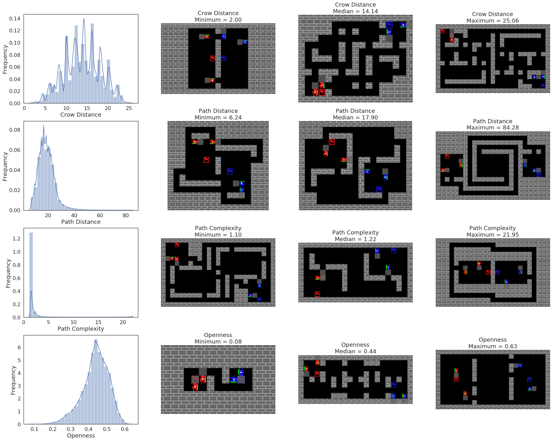
To demonstrate the diversity of the procedurally generated levels for Capture the Flag, this section introduces four descriptive features, presents their distributions from 100,000 samples, and visualizes the minimum, medium, and maximum level of each distribution.
The four features are as follows:
-
1.
Crow Distance: The euclidean distance between the red flag and blue flag.
-
2.
Path Distance: The path distance between the red flag and blue flag.
-
3.
Path Complexity: The crow distance divided by the path distance.
-
4.
Openness: The proportion of non-wall cells in the level.
Example levels
Presented in Figure A13 are 12 randomly sampled levels generated by the previously described procedure.

Appendix B Agents
B.1 Training and evaluation
We use a distributed asynchronous training framework consisting of “arenas” that run in parallel to train populations of reinforcement learning agents. In Tables A3 and Table A4, we provide details of this experimental setup:
| Setting | HarvestPatch | Traffic Navigation | Overcooked | Capture the Flag | |
|---|---|---|---|---|---|
| Game type | mixed-motive | coordination | common-payoff | competitive | |
| # players (players ) | 6 | 8 | 2 | 4 (2 versus 2) | |
| # training steps per agent | 1e9 | 5e8 | 3e9 | 3e9 | |
| training time per experiment | 1 day | 12 hours | 3 days | 3 days | |
| # steps per episode | 1000 | 1000 | 540 | 2400 | |
| Setting | Value | |
|---|---|---|
| # agents (population size ) | {1, 2, 4, 8} for HarvestPatch, Traffic Navigation, Overcooked; | |
| {1, 2, 4, 8, 16} for Capture the Flag | ||
| # levels (training levels ) | {1, 1e1, 1e2, 1e3, 1e4} | |
| sample agents with replacement? | yes | |
| # arenas | {200, 400, 800, 1600, 1600} for , respectively | |
| # GPUs per agent | 1 | |
B.2 V-MPO
B.2.1 Architecture and hyperparameters
We used the following architecture for V-MPO song2019v . The agent’s visual observations were first processed through a 3-section ResNet used in hessel2019multi . Each section consisted of a convolution and max-pooling operation (stride 2), followed by residual blocks of size 2 (i.e., a convolution followed by a ReLU nonlinearity, repeated twice, and a skip connection from the input residual block input to the output). The entire stack was passed through one more ReLU nonlinearity. All convolutions had a kernel size of 3 and a stride of 1. The number of channels in each section was (16, 32, 32).
The resulting output was then concatenated with the previous action and reward of the agent (along with any extra observations in Capture the Flag and Traffic Navigation), and processed by a single-layer MLP with 256 hidden units. This was followed by a single-layer LSTM with 256 hidden units (unrolled for 100 steps), and then a separate single-layer MLP with 256 hidden units to produce the action distribution. For the critic, we used a single-layer MLP with 256 hidden units followed by PopArt normalization (ablated in Section B.2.2).
To train the agent, we used a discount factor of 0.99, batch sizes of 16, and the Adam optimizer (kingma2014adam ; learning rate of 0.0001). We configured V-MPO with a target network update period of 100, , and an epsilon temperature of 0.1. For PopArt normalization, we used a scale lower bound of , an upper bound of , and a learning rate of .
B.2.2 PopArt normalization
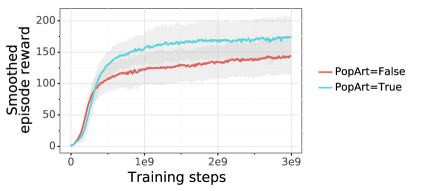
PopArt normalization is typically used in multi-task settings hessel2019multi . While we did not investigate multi-task settings in this work, we found that including PopArt (as in song2019v ) led to improved performance on the procedurally generated environments considered here. In Figure A14, we show the reward curves across training on both the training and test levels with PopArt normalization enabled (PopArt = True) and disabled (PopArt = False). As can be seen, PopArt consistently leads to a higher reward and therefore more performant agents. Consequently, we used PopArt for all agents.
B.2.3 Social Value Orientation
For the “identical” populations of Social Value Orentation agents, we set the target reward angle hyperparameter with an identical distribution across agents: . For the “heterogeneous” populations of Social Value Orientation agents, is set with a diverse distribution across agents: .
Appendix C Methods
C.1 Expected action variation
For reproducibility, we include pseudocode to calculate expected action variation (Algorithm 1). Starting from a set of populations of interest trained on a shared set of levels , we simulate a number of episodes within each population to generate a representative pool of agent states (Algorithm 2). We then approximate action-policy distributions over these states for each agent in each population (Algorithm 3). Finally, for each population, we compare the action-policy distributions between each pair of agents within the population to calculate that population’s expected action variation (Algorithm 4).
Because the environments that we consider in this paper use discrete action spaces, Algorithm 4 uses total variation distance to estimate pairwise divergence between action-policy distributions. For environments with continuous action spaces, pairwise divergence could be estimated with earth mover’s distance instead.
C.2 Calculating Elo rating
To calculate the Elo rating of each trained population, we evaluate every possible pairing of trained populations against each another with 100 matches per pairing. For each of these 100 matches, two agents are randomly sampled from the first population to form the red team, and two from the second population to form the blue team (sampling with replacement).
After these matches are completed, we iteratively calculate the Elo rating of each population using the following procedure on each match result (looping over all match results until convergence):
where we initialised the rating of each population to 1000 and set .
Appendix D Additional Results
This section presents additional results and statistical analyses supporting the results in the main text.
For each ANOVA we conducted, we compare the categorical levels of the independent variable in pairs and apply Tukey’s honestly significant differences (HSD) method to evaluate which pairs differ significantly tukey1949comparing . Tukey’s method adjusts the raw -values to account for the increased probability of false positives when running multiple independent statistical tests.
D.1 Environment Diversity
D.1.1 Generalization Gap Analysis
HarvestPatch
| Individual reward on: | Gen. gap | ||
|---|---|---|---|
| Train levels | Test levels | (train test) | |
| () | () | () | |
| () | () | () | |
| () | () | () | |
| () | () | () | |
| () | () | () | |
| Mean difference | Adjusted -value | ||
|---|---|---|---|
Traffic Navigation
| Individual reward on: | Gen. gap | ||
|---|---|---|---|
| Train levels | Test levels | (train test) | |
| () | () | () | |
| () | () | () | |
| () | () | () | |
| () | () | () | |
| () | () | () | |
| Mean difference | Adjusted -value | ||
|---|---|---|---|
Overcooked
| Individual reward on: | Gen. gap | ||
|---|---|---|---|
| Train levels | Test levels | (train test) | |
| () | () | () | |
| () | () | () | |
| () | () | () | |
| () | () | () | |
| () | () | () | |
| Mean difference | Adjusted -value | ||
|---|---|---|---|
Capture the Flag
| Individual reward on: | Gen. gap | ||
|---|---|---|---|
| Train levels | Test levels | (train test) | |
| () | () | () | |
| () | () | () | |
| () | () | () | |
| () | () | () | |
| () | () | () | |
| Mean difference | Adjusted -value | ||
|---|---|---|---|
D.1.2 Cross-Play Evaluation
Capture the Flag
D.2 Population Diversity
D.2.1 Expected Action Variation
All environments
| Expected Action Variation | ||||
|---|---|---|---|---|
| HarvestPatch | Traffic Navigation | Overcooked | Capture the Flag | |
| () | () | () | () | |
| () | () | () | () | |
| () | () | () | () | |
| () | () | () | () | |
| – | – | – | () | |
HarvestPatch
| Mean difference | Adjusted -value | ||
|---|---|---|---|
Traffic Navigation
| Mean difference | Adjusted -value | ||
|---|---|---|---|
Overcooked
| Mean difference | Adjusted -value | ||
|---|---|---|---|
Capture the Flag
| Mean difference | Adjusted -value | ||
|---|---|---|---|
Intrinsic Motivation and Behavioral Diversity
| Social Value Orientation | Expected Action Variation |
|---|---|
| None | 0.30 (0.02) |
| Identical | 0.30 (0.03) |
| Diverse | 0.37 (0.01) |
| Mean difference | Adjusted -value | ||
|---|---|---|---|
| None | Identical | ||
| None | Diverse | ||
| Identical | Diverse |
D.2.2 Cross-Play Evaluation
HarvestPatch
| Individual reward on: | |
|---|---|
| Training level | |
| () | |
| () | |
| () | |
| () |
| Mean difference | Adjusted -value | ||
|---|---|---|---|
Traffic Navigation
| Individual reward on: | |
|---|---|
| Training level | |
| () | |
| () | |
| () | |
| () |
| Mean difference | Adjusted -value | ||
|---|---|---|---|
Overcooked
| Individual reward on: | |
|---|---|
| Training level | |
| () | |
| () | |
| () | |
| () |
| Mean difference | Adjusted -value | ||
|---|---|---|---|
Capture the Flag
