Demarcating Endogenous and Exogenous Opinion Dynamics: An Experimental Design Approach

Abstract.

The networked opinion diffusion in online social networks (OSN) is often governed by the two genres of opinions— endogenous opinions that are driven by the influence of social contacts among users, and exogenous opinions which are formed by external effects like news, feeds etc. Accurate demarcation of endogenous and exogenous messages offers an important cue to opinion modeling, thereby enhancing its predictive performance. In this paper, we design a suite of unsupervised classification methods based on experimental design approaches, in which, we aim to select the subsets of events which minimize different measures of mean estimation error. In more detail, we first show that these subset selection tasks are NP-Hard. Then we show that the associated objective functions are weakly submodular, which allows us to cast efficient approximation algorithms with guarantees. Finally, we validate the efficacy of our proposal on various real-world datasets crawled from Twitter as well as diverse synthetic datasets. Our experiments range from validating prediction performance on unsanitized and sanitized events to checking the effect of selecting optimal subsets of various sizes. Through various experiments, we have found that our method offers a significant improvement in accuracy in terms of opinion forecasting, against several competitors.

1. Introduction

Research on understanding opinion dynamics, from both modeling and control perspectives, abounds in literature (Clifford and Sudbury, 1973; DeGroot, 1974; Dittmer, 2001; Holme and Newman, 2006; Blondel et al., 2009; Douven and Riegler, 2009; Yildiz et al., 2010; Mor et al., 2011; Das et al., 2014; De et al., 2014; Altafini and Lini, 2015; Etesami and Başar, 2015; Friedkin, 2015; Morărescu et al., 2016; De et al., 2016), predominantly following two approaches. The first approach is grounded on the concepts of statistical physics, it is barely data-driven and therefore shows poor predictive performance (Clifford and Sudbury, 1973; DeGroot, 1974; Dittmer, 2001; Holme and Newman, 2006; Blondel et al., 2009; Douven and Riegler, 2009; Yildiz et al., 2010; Mor et al., 2011; Altafini and Lini, 2015; Etesami and Başar, 2015; Friedkin, 2015; Morărescu et al., 2016), The second class of models aims to overcome such limitations, by learning a tractable linear model from transient opinion dynamics (De et al., 2014; Das et al., 2014; De et al., 2016). Barring the individual limitations of these existing approaches, they all have assumed the absence or lack of external effects, despite empirical evidences advocating the presence of such signals (Grabowicz et al., 2016; Myers et al., 2012; Anagnostopoulos et al., 2008; Greenhalgh et al., 2004; Valente, 1996). Since a social network is an open system encouraging both inward and outward flow of information, a continuous flux of external information is funneled to its users, via a gamut of sources like news, feeds, etc. As a result, a networked opinion formation process that involves extensive interactive discussions among connected users, is also propelled by such external sources recommended to those users. Therefore, at the very outset, we observe two families of opinions – endogenous opinions which evolve due to the influence from neighbors, and exogenous opinions that are driven mostly by the externalities. In most practical situations, the true labels of the posts (endogenous or exogenous) are not available. Therefore, an accurate unsupervised labeling of the posts has immense potential impact on opinion modeling – boosting the predictive performance for a broad spectrum of applications like pole-prediction, brand sentiment estimation, etc. In this paper, our goal is to demarcate endogenous and exogenous messages and demonstrate the utility of our proposal from an opinion modeling viewpoint.

1.1. Proposed approach

We initiate investigating the dynamics of organic opinion in the presence of exogenous actions, using a recent temporal point-process based model SLANT (De et al., 2016). It allows users’ latent endogenous opinions to be modulated over time, by both endogenous and exogenous opinions of their neighbours, expressed as sentiment messages (Section 3).

Subsequently, in Section 4 we propose CherryPick , a suite of learning algorithms, based on experimental design methods that optimally demarcate the endogenous and exogenous opinions under various circumstances. In a nutshell, in order to categorize messages, we aim to select the set of events that comply with the organic dynamics with a high confidence, i.e. a low variance of influence estimation. To this end, we devise this problem as an inference task of the message category (endogenous or exogenous) by means of subset selection (i.e. demarcating a subset of endogenous messages from the whole message stream). We find that this proposed inference problem can be formulated as an instance of a cardinality constrained submodular maximization problem. To solve this optimization problem, we present a greedy approach which, like an ordinary greedy submodular maximization algorithm, enjoys approximation bounds. However, since some of the optimization objectives we consider are only weakly submodular, they admit some special approximation bounds which have been proposed recently in (Hashemi et al., 2019).

Finally, we perform experiments on various real datasets, crawled from Twitter about diverse topics (Section 5) and synthetic datasets, built over diverse networks (Section 6) and show that CherryPick can accurately classify endogenous and exogenous messages, thereby helping to achieve a substantial performance boost in forecasting opinions.

2. Related Work

Opinion modeling and its applications have been widely studied in different guises in many years. In this section, we review some of them, from two major perspectives– (i) opinion dynamics modeling and (ii) opinion sensing.

Opinion dynamics modeling. Modeling the evolution process of opinion flow over networks, mostly follows two approaches, based on (a) statistical physics and (b) data-driven techniques. The first type of models, e.g. Voter, Flocking, DeGroot, etc. is traditionally designed to capture various regulatory real-life phenomena e.g. consensus, polarization, clustering, coexistence etc. (Clifford and Sudbury, 1973; Yildiz et al., 2013; Schweitzer and Behera, 2009; Yildiz et al., 2010; Vazquez et al., 2003; Castelló et al., 2006; Medeiros et al., 2006; Mobilia, 2003; Vazquez and Eguíluz, 2008; Durrett and Levin, 1996; DeGroot, 1974; Hegselmann and Krause, 2002; Krause, 2000; Deffuant et al., 2000; Weisbuch et al., 2002). Voter model (Clifford and Sudbury, 1973) is a discrete opinion model, where opinions are represented as nominal values, and copied from influencing neighbors in every step. This underlying principle is still a major workhorse for many discrete opinion models (Yildiz et al., 2013; Schweitzer and Behera, 2009; Yildiz et al., 2010; Vazquez et al., 2003; Castelló et al., 2006; Medeiros et al., 2006; Mobilia, 2003; Vazquez and Eguíluz, 2008; Durrett and Levin, 1996). In contrast to these models, Flocking and DeGroot are continuous opinion models. In Flocking model and its variations (Hegselmann and Krause, 2002; Krause, 2000; Deffuant et al., 2000; Weisbuch et al., 2002), a node $i$ having opinion $x_{i}$ first selects the set of neighbors $j$ with $|x_{i}-x_{j}|\leq\epsilon$, and then updates its own opinion by averaging these opinions. DeGroot model (DeGroot, 1974), on the other hand, allows a user to update her opinion with the average opinions of all her neighbors. In this model, the underlying influence matrix is row stochastic, enforcing consensus for a strongly connected graph. The second class of models, e.g. Biased Voter, AsLM, SLANT, etc. aim to learn a tractable linear model from a temporal message stream reflecting transient opinion dynamics (Das et al., 2014; De et al., 2014, 2016; Gupta et al., 2021). While a Biased Voter model (Das et al., 2014) unifies various aspects of DeGroot and Flocking models, AsLM (De et al., 2014) generalizes the DeGroot model by relaxing the structure of the influence matrix. In contrast to these models that ignore the temporal effects of messages (post-rate), SLANT (De et al., 2016) blends the opinion dynamics along with the message dynamics, using a stochastic generative model. In contrast to the above modeling approaches, there exist abundant empirical studies (Centola, 2010; Aral and Walker, 2011; Bakshy et al., 2012b, a; Friggeri et al., 2014) which investigate various factors influencing information diffusion in social networks through large-scale field experiments. However, all these approaches skirt the effect of externalities, which severely constrains their forecasting prowess.

Opinion sensing. Sensing opinions, or mining sentiments from textual data traditionally relies on sophisticated NLP based machineries. See (Liu, 2012; Pang and Lee, 2008) for details. Both these monographs provide a comprehensive survey. In general, LIWC (Pennebaker et al., 2001) is widely considered as benchmark tool to compute sentiments from rich textual data. On the other hand, Hannak et al. developed a simple yet effective method for sentiment mining from short informal text like tweets (Hannak et al., 2012), also used by  (De et al., 2014, 2016). Recently, a class of works (Li et al., 2015; Hosseinia and Mukherjee, 2017; KC and Mukherjee, 2016; Li et al., 2017) designs simple supervised strategies to sense opinion spams, and some of them (Hosseinia and Mukherjee, 2017; KC and Mukherjee, 2016; Li et al., 2017) also advocate the role of temporal signals in opinion spamming. Note that, exogenous opinions are fundamentally different from opinion spams. In contrast to a spam which is unsolicited and irrelevant to the discussion, an exogenous post is often relevant, yet just an informed reflection of some external news or feeds. Also, since spamminess of a message is its intrinsic property, it does not depend on the messages before it. However, an exogenous post when retweeted, can become endogenous. Furthermore, the opinion spam detection techniques rest on the principle of supervised classification that in turn requires labeled messages. However, in the context of networked opinion dynamics, the messages (tweets) come unlabeled, which renders the spam detection techniques practically inapplicable for such scenarios.

Finally we conclude this section with this note that our work closely resembles SLANT (De et al., 2016) and is built upon the modeling framework proposed by SLANT, but the major difference is that SLANT assumes the entire event stream as endogenous, whereas our work is motivated towards exploring various techniques for systematically demarcating the externalities from the heterogeneous event stream. Similarly, our proposed algorithms are closely influenced by recent progress in subset selection literature (Hashemi et al., 2019) where authors deal with designing new alphabetical optimality criteria for quadratic models. However, our work is motivated towards investing the subset selection problem for linear models in a temporal setting.

3. Problem setup

In what follows, we describe the scenario of a social network of users who post opinion-bearing messages. For ease of reference, we list a compendium of all important notations used in this section in Table 1.

Symbol	Meaning
$\mathcal{G}$	A directed social network (such as Twitter)
$\mathcal{V}$	Vertices of $\mathcal{G}$ (users)
$\mathcal{E}$	Edges of $\mathcal{G}$ (follower-followee links)
$\mathcal{N}(u)$	Set of users followed by $u$, subset of $\mathcal{V}$
$\mathcal{U}(t)$	History of messages posted by all users until time $t$
$\mathcal{U}_{u}(t)$	History of messages posted by user $u$ until time $t$
$e_{i}$	$i$th message in $\mathcal{U}(t)$
$u_{i}$	User posting the $i$th message in $\mathcal{U}(t)$
$\zeta_{i}$	Opinion/sentiment value of the $i$th message in $\mathcal{U}(t)$
$t_{i}$	Timestamp of the $i$th message in $\mathcal{U}(t)$
$\mathcal{H}(t)$	Set of endogenous messages in $\mathcal{U}(t)$
$m_{i}$	Opinion/sentiment value of the $i$th endogenous message in $\mathcal{H}(t)$
$\mathcal{H}_{u}(t)$	Set of endogenous messages posted by user $u$ in $\mathcal{U}_{u}(t)$
$\mathcal{C}(t)$	Set of exogenous messages in $\mathcal{U}(t)$, complementary to $\mathcal{H}(t)$
$w_{i}$	Opinion/sentiment value of the $i$th exogenous message in $\mathcal{C}(t)$
$\mathcal{C}_{u}(t)$	Set of exogenous messages posted by user $u$ in $\mathcal{U}_{u}(t)$, complementary to $\mathcal{H}_{u}(t)$
$N_{u}(t)$	Counting process for endogenous messages of user $u$, equal to $|\mathcal{H}_{u}(t)|$
$M_{u}(t)$	Counting process for endogenous messages of user $u$, equal to $|\mathcal{C}_{u}(t)|$
$\bm{N}(t)$	Set of counting processes $(\leavevmode\nobreak\ N_{u}(t)\leavevmode\nobreak\ )_{u\in\mathcal{V}}$
$\bm{M}(t)$	Set of counting processes $(\leavevmode\nobreak\ M_{u}(t)\leavevmode\nobreak\ )_{u\in\mathcal{V}}$
$\lambda_{u}^{*}(t)$	Intensity of $N_{u}(t)$, i.e. the endogenous message rate of user $u$
$\bm{\lambda}^{*}(t)$	Set of intensities $(\leavevmode\nobreak\ \lambda_{u}^{*}(t)\leavevmode\nobreak\ )_{u\in\mathcal{V}}$

Table 1. List of important notations used in Section 3.

We use two sources of data as input: (I). a directed social network $\mathcal{G}=(\mathcal{V},\mathcal{E})$ of users with the connections between them (e.g. friends, following, etc), and (II). an aggregated history $\mathcal{U}(T)$ of the messages posted by these users during a given time-window $[0,T)$. In this paper, we summarize each message-event $e_{i}\in\mathcal{U}(T)$ using only three components, the user $u_{i}$ who has posted the message, the opinion or sentiment value $\zeta_{i}$ associated with the message, and the timestamp $t_{i}$ of the post. Therefore, $\mathcal{U}(T):=\{e_{i}=(u_{i},\zeta_{i},t_{i})|t_{i}<T\}$. We also use the notation $\mathcal{U}(t)$ to denote the set of messages collected until $t<T$ i.e. $\mathcal{U}(t):=\{e_{i}=(u_{i},\zeta_{i},t_{i})|t_{i}<t\}$.

In the spirit of (De et al., 2016), we assume that the history of events until time $t$ influences the arrival process of events after time $t$. However, in a direct contrast to (De et al., 2016) which skirts the potential influence of externalities, we posit that the message events belong to two categories– endogenous and exogenous. Whereas the arrivals of endogenous events are driven by the previous events in the network i.e. these are history-dependent, exogenous events originate from external influence outside the given social network and are, therefore not history-dependent. Note that the distinction between endogenous and exogenous events is not directly observable from the data, but needs to be inferred from the characteristics of the event sequence. To this end, we split the entire set of messages observed until time $t$, $\mathcal{U}(t)$ into two complementary subsets, $\mathcal{H}(t)$ and $\mathcal{C}(t)$ representing the sets of endogenous and exogenous events respectively, with $\mathcal{U}(t)=\mathcal{H}(t)\cup\mathcal{C}(t)$ & $\mathcal{H}(t)\cap\mathcal{C}(t)$ = $\phi$. At a user level, we denote $\mathcal{H}_{u}(t)=\{e_{i}=(u_{i},m_{i},t_{i})|u_{i}=u\ \mbox{and}\,t_{i}<t\}$ as the collection of all endogenous messages with sentiments $m_{i}$, posted by user $u$ until time $t$. Similarly, $\mathcal{C}_{u}(t)=\{e_{i}=(u_{i},w_{i},t_{i})|u_{i}=u\ \mbox{and}\,t_{i}<t\}$ denotes the history of exogenous messages posted by user $u\in\mathcal{V}$ with sentiments $w_{i}$ until time $t$. Finally we write $\mathcal{U}_{u}(t)=\mathcal{H}_{u}(t)\cup\mathcal{C}_{u}(t)$, as the history gathering both types of messages posted by user $u$, until time $t$. Therefore, $\cup_{u\in\mathcal{V}}\mathcal{H}_{u}(t)=\mathcal{H}(t)$, $\cup_{u\in\mathcal{V}}\mathcal{C}_{u}(t)=\mathcal{C}(t)$, and $\cup_{u\in\mathcal{V}}\mathcal{U}_{u}(t)=\mathcal{U}(t)$. Note that, for clarity we denote $m_{i}$ and $w_{i}$ as endogenous and exogenous sentiments respectively, while $\zeta_{i}$ denotes opinion of any type. However, both types of sentiments belong to identical domain. To model the endogenous message dynamics, we represent the message times by a set of counting processes denoted as a vector $\bm{N}(t)$, in which the $u$-th entry, $N_{u}(t)\in\left\{0\right\}\cup\mathbb{Z}^{+}$, counts the number of endogenous messages user $u$ posted until time $t$, i.e. $N_{u}(t)=|\mathcal{H}_{u}(t)|$. Then, we characterize the message rates with the conditional intensity function

(1) $$\mathbb{E}[d\bm{N}(t)\,|\,\mathcal{U}(t)]=\bm{\lambda}^{*}(t)\,dt,$$

where $d\bm{N}(t):=\left(\leavevmode\nobreak\ dN_{u}(t)\leavevmode\nobreak\ \right)_{u\in\mathcal{V}}$ counts the endogenous messages per user in the interval $[t,t+dt)$ and $\bm{\lambda}^{*}(t):=(\leavevmode\nobreak\ \lambda_{u}^{*}(t)\leavevmode\nobreak\ )_{u\in\mathcal{V}}$ denotes the user intensities that depend on the history $\mathcal{U}(t)$.

Note that we assume the endogenous events do not depend on their own history $\mathcal{H}(t)$ only, but rather on the combined history $\mathcal{U}(t)$ of both endogenous and exogenous events. Hence, every exogenous post influences the subsequent endogenous events in the same manner as the previous endogenous events. This is because a recipient user cannot distinguish between exogenous or endogenous posts made by her neighbors.

In order to represent the arrival times of the exogenous message set $\mathcal{C}(t)$, we introduce an additional counting process $\bm{M}(t)$ that describes the rate of generation of exogenous events, in which the $u$-th entry, $M_{u}(t)\in\left\{0\right\}\cup\mathbb{Z}^{+}$, counts the number of exogenous messages user $u$ posted until time $t$, i.e. $M_{u}(t)=|\mathcal{C}_{u}(t)|$. Note that, we do not aim to model the dynamics of exogenous events, since their source is not known to us.

3.1. Opinion dynamics in absence of exogenous actions

For clarity, we briefly discuss the proposal by De et al. (De et al., 2016), that ignores the effect of exogenous messages. The user intensities $\lambda_{u}^{*}(t)$ are generally modeled using multivariate Hawkes Process (Liniger, 2009). We denote the set of users that u follows by $\mathcal{N}(u)$. In absence of exogenous actions, i.e., when $\mathcal{U}(t)=\mathcal{H}(t)$, we have:

(2) $$\lambda^{*}_{u}(t)=\mu_{u}+\sum_{v\in\mathcal{N}(u)}b_{vu}\sum_{e_{i}\in\mathcal{H}_{v}(t)}\kappa(t-t_{i}).$$

Here, the first term, $\mu_{u}\geqslant 0$, captures the posts by user $u$ on her own initiative, and the second term, with $b_{vu}\geqslant 0$, reflects the influence of previous posts on her intensity (self-excitation). The users’ latent opinions are represented as a history-dependent, multidimensional stochastic process $\mathbf{x}^{*}(t)$:

(3) $$x^{*}_{u}(t)=\alpha_{u}+\sum_{v\in\mathcal{N}(u)}a_{vu}\sum_{e_{i}\in\mathcal{H}_{v}(t)}m_{i}g(t-t_{i})$$

where the first term, $\alpha_{u}\in\mathbb{R}$, models the original opinion of a user $u$ and the second term, with $a_{vu}\in\mathbb{R}$, models updates in user $u$’s opinion due to the influence from previous messages of her neighbours. Here, $\kappa(t)=e^{-\nu t}$ and $g(t)=e^{-\omega t}$ (where $\nu,\ \omega\geqslant 0$) denote exponential triggering kernels, which model the decay of influence over time. Finally, when a user $u$ posts a message at time $t$, the message sentiment $m$ reflects the expressed opinion which is sampled from a distribution $p(m|x^{*}_{u}(t))$. Here, the sentiment distribution $p(m|x^{*}_{u}(t))$ is assumed to be normal, i.e. $p(m|x_{u}(t))=\mathcal{N}(x_{u}(t),\sigma_{u})$.

3.2. Opinion dynamics with exogenous events

In this section, we model the effect of exogenous events, $\mathcal{C}(t)$, on the latent endogenous opinion process $x^{*}(t)$ and the endogenous rate $\lambda^{*}(t)$. Recall that $\mathcal{N}(u)$ denotes the set of users that u follows. We present the dynamics of latent opinion $x^{*}_{u}(t)$ of user $u$, in the presence of exogenous messages in the following equation.

(4) $$x^{*}_{u}(t)=\alpha_{u}+\sum_{v\in\mathcal{N}(u)}a_{vu}\Big{(}\sum_{e_{i}\in\mathcal{H}_{v}(t)}m_{i}g(t-t_{i})+\sum_{e_{i}\in\mathcal{C}_{v}(t)}w_{i}g(t-t_{i})\Big{)}$$

where, the last term captures signals from exogenous posts. Similarly, the endogenous message rate $\lambda_{u}^{*}(t)$ of a user $u$ evolves as,

(5) $$\lambda^{*}_{u}(t)=\mu_{u}+\sum_{v\in\mathcal{N}(u)}b_{vu}\Big{(}\sum_{e_{i}\in\mathcal{H}_{v}(t)}\kappa(t-t_{i})+\sum_{e_{i}\in\mathcal{C}_{v}(t)}\kappa(t-t_{i})\Big{)}.$$

Note that same parameters, $a_{vu}$ and $b_{vu}$, are used to model the effect of endogenous and exogenous processes, on both opinion and message dynamics. The above equation can be equivalently written as:

(6) $$\bm{x}^{*}(t)=\bm{\alpha}+\int_{0}^{t}g(t-s)\bm{A}\big{[}\bm{m}(s)\odot d\bm{N}(s)+\bm{w}(s)\odot d\bm{M}(s)\big{]}$$

(7) $$\bm{\lambda}^{*}(t)=\bm{\mu}+\int_{0}^{t}\bm{B}\kappa(t-s)\big{[}d\bm{N}(s)+d\bm{M}(s)\big{]}.$$

Here $\bm{A}=(a_{vu})\in\mathbb{R}^{|\mathcal{V}|\times|\mathcal{V}|}$, $\bm{B}=(b_{vu})\in\mathbb{R}^{|\mathcal{V}|\times|\mathcal{V}|}_{+}$, $\bm{x}^{*}(t)=(x^{*}_{u}(t))_{u\in\mathcal{V}}$. Similarly we define $\bm{\lambda}^{*}(t),\ \bm{m}(s),\ \bm{w}(s)$. Furthermore, the exogenous intensity is given by: $\mathbb{E}[d\bm{M}(t)|\mathcal{U}(t)]=\bm{\eta}(t)$. We do not aim to model $\bm{\eta}(t)$.

By defining, $\bm{P}(t):=\bm{N}(t)+\bm{M}(t)$, as the counting process associated with the combined history $\mathcal{U}(t)=\mathcal{H}(t)\cup\mathcal{C}(t)$ of both endogenous and exogenous events, we further simplify Eqs. (6) and  (7) as,

(8) $$\bm{x}^{*}(t)=\bm{\alpha}+\int_{0}^{t}g(t-s)\bm{A}\big{[}\bm{\zeta}(s)\odot d\bm{P}(s)\big{]}$$

(9) $$\bm{\lambda}^{*}(t)=\bm{\mu}+\int_{0}^{t}\bm{B}\kappa(t-s)d\bm{P}(s).$$

4. Demarcation of endogenous and exogenous messages

In this section, we propose a novel technique for demarcating endogenous messages $\mathcal{H}(T)$ and exogenous messages $\mathcal{C}(T)$ from a stream of unlabelled messages $\mathcal{U}(T)$ gathered during time $[0,T)$. Then, based on the categorized messages, we find the optimal parameters $\bm{\alpha}$, $\bm{\mu}$, $\bm{A}$ and $\bm{B}$ by solving a maximum likelihood estimation (MLE) problem. From now onwards, we would write $\mathcal{U}(T)$, $\mathcal{H}(T)$, $\mathcal{C}(T)$ as $\mathcal{U}_{T}$, $\mathcal{H}_{T}$ and $\mathcal{C}_{T}$ to lighten the notations. Hence, succinctly, the problem can be stated as follows:

1. identify a subset $\mathcal{H}_{T}\subseteq\mathcal{U}_{T}$ of endogenous events

2. find the optimal (maximum-likelihood) parameters $\bm{\alpha}$, $\bm{\mu}$, $\bm{A}$ and $\bm{B}$ based only on $\mathcal{H}_{T}$

4.1. CherryPick_X: Our proposed approach

Now, we attempt to design an unsupervised learning algorithm to isolate the endogenous events $\mathcal{H}_{T}$ and exogenous events $\mathcal{C}_{T}$ from the stream of unlabeled sentiment messages $\mathcal{U}_{T}$, which is equivalent to assigning each event $e\in\mathcal{U}_{T}$ into either $\mathcal{H}_{T}$ or $\mathcal{C}_{T}$. This is achieved by extracting the set of events that comply with the endogenous dynamics with high confidence that in turn is indicated by a low variance of estimated parameters.

In more detail, given a candidate set of endogenous events $\mathcal{H}_{T}$, the opinion parameters $\bm{A},\bm{\alpha}$ can be estimated by maximizing the likelihood of endogenous opinions $m_{i}$, $\sum_{i}\log p(m_{i}|x^{*}_{u_{i}}(t_{i}))$, i.e., minimizing the following,

$$\underset{\bm{A},\bm{\alpha}}{\text{min}} \sum_{\begin{subarray}{c}\ e_{i}\in\mathcal{H}_{T}\\ u\in\mathcal{V}\end{subarray}}\sigma^{-2}\Big{(}m_{i}-\alpha_{u}-\int_{0}^{t_{i}}g(t-s)(\bm{\zeta}(s)\odot d\bm{P}(s))^{T}\bm{A}_{u}\Big{)}^{2}\Big{.}$$

(10) $$+c||\bm{A}||_{F}^{2}+c||\bm{\alpha}||_{2}^{2}.$$

Here, the first term is derived using the Gaussian nature of $p(m|x^{*}_{u}(t))$ and the last two are the regularized terms. The optimal parameters ($\hat{\bm{A}},\ \hat{\bm{\alpha}}$) depend on the candidate set of endogenous messages $\mathcal{H}_{T}$. To this end, we compute the estimation covariance as,

(11) $$\bm{\Sigma}(\mathcal{H}_{T}):=\mathbb{E}(\hat{\bm{\theta}}-\bm{\theta})(\hat{\bm{\theta}}-\bm{\theta})^{T},\ \bm{\theta}:=\text{vec}([\bm{A},\ \bm{\alpha}]).$$

Here the expectation is taken over the noise process induced while getting the message sentiment $m_{i}$, from the opinion $x_{u_{i}}^{*}(t_{i})$ according to the distribution $p(m_{i}|x^{*}_{u_{i}}(t_{i}))$. Before proceeding further, we want to make a clarification that we exclude intensity parameters ($\mu$ and $B$) in covariance estimation as their MLE estimation do not offer closed form solution, making it mathematically inconvenient. Prior to going into the selection mechanism of $\mathcal{H}_{T}$, we first look into the expression of covariance matrix $\bm{\Sigma}$ in the Lemma 4.1. Note that, the inference problem given by Eq. (10) is that of regularized least squares estimation, and so the covariance matrix for the optimal parameters can be derived in a closed form given in the following:

Lemma 4.1.

For a given endogenous message-set $\mathcal{H}_{T}$,

(12) $$\bm{\Sigma}(\mathcal{H}_{T})=\mathop{\mathrm{diag}}_{u\in\mathcal{V}}\big{(}c\bm{I}+\sigma^{-2}\sum_{e_{i}\in\mathcal{H}_{T}}\bm{\phi}^{u}_{i}\bm{\phi}_{i}^{uT}\big{)}^{-1}$$

where,

(13) $$\bm{\phi}^{u}_{i}=\begin{cases}\text{vec}([\int_{0}^{t_{i}}g(t-s)\bm{\zeta}(s)\odot d\bm{P}(s),1])&u_{i}=u\\ 0&u_{i}\neq u\end{cases}$$

The proof of this lemma is given in the Appendix (Section A.1).

Our objective is to identify $\mathcal{H}_{T}$, given its size $N_{\mathcal{H}}$, so that $\bm{\Sigma}(\mathcal{H}_{T})$ is small. Such a demarcated message-set $\mathcal{H}_{T}$ would then follow endogenous opinion dynamics more faithfully than its complement $\mathcal{U}_{T}\backslash\mathcal{H}_{T}$. In order to compute the best candidate for $\mathcal{H}_{T}$, we need to minimize a suitable function $\Omega_{X}(\mathcal{H}_{T})$ which is some measure of $\bm{\Sigma}(\mathcal{H}_{T})$.

In accordance with the alphabetical design criteria of A-optimality, D-optimality, E-optimality, and T-optimality used by (Hashemi et al., 2019; Chaloner and Verdinelli, 1995), we define,

(14) $$\Omega_{A}(\mathcal{H}_{T}):=\mathop{\mathrm{tr}}\left[\bm{\Sigma}(\mathcal{H}_{T})\right]$$

(15) $$\Omega_{D}(\mathcal{H}_{T}):=\mathop{\mathrm{tr}}\left[\log\bm{\Sigma}(\mathcal{H}_{T})\right]=\log\left[\mbox{det}(\bm{\Sigma}(\mathcal{H}_{T}))\right]$$

(16) $$\Omega_{E}(\mathcal{H}_{T}):=\lambda_{max}\left[\bm{\Sigma}(\mathcal{H}_{T})\right]$$

(17) $$\Omega_{T}(\mathcal{H}_{T}):=-\mathop{\mathrm{tr}}\left[\bm{\Sigma}(\mathcal{H}_{T})^{-1}\right]$$

where $\log\bm{\Sigma}$ is the matrix logarithm of $\bm{\Sigma}$, and $\lambda_{max}\left[\bm{\Sigma}(\mathcal{H}_{T})\right]$ refers to the maximum eigenvalue of $\bm{\Sigma}(\mathcal{H}_{T})$. These functions $\Omega_{X}(\mathcal{H}_{T})$, where $X\in\{A,D,E,T\}$ can be viewed as complexity measures of $\bm{\Sigma}(\mathcal{H}_{T})$ (Hashemi et al., 2019) that make them good candidates for minimizing $\bm{\Sigma}$. Hence, by defining $f_{X}(\mathcal{H}_{T}):=-\Omega_{X}(\mathcal{H}_{T})$, where $X\in\{A,D,E,T\}$, we pose the following optimization problem to obtain the best cardinality constrained candidate set $\mathcal{H}_{T}$:

$$\underset{\mathcal{H}_{T}\in\mathcal{U}_{T}}{\text{maximize}}f_{X}(\mathcal{H}_{T})$$

(18) $$\text{subject to, }|\mathcal{H}_{T}|=N_{\mathcal{H}}$$

Normally such a cardinality constrained subset selection problem would be NP-Hard (Williamson and Shmoys, 2011; Krause and Golovin, 2014). Hence, we will rely on a greedy heuristic for maximizing $f_{X}$ (Algorithm 1), that, we would show later, gives an $(1-1/e)$ approximation bound. Before going to that, we first specify two properties defined for any set function $h(V)$ in general (Definition 4.2) . We would show that, $f_{X}$ specifically enjoys these properties, thereby affording an approximation guarantee from the proposed simple greedy algorithm.

Definition 4.2.

A multidimensional set function $h(V)$ in a set argument $V\subseteq U$, is said to be

1. submodular, if for any set $V\subseteq\overline{V}$, $x\not\in\overline{V}$

   (19) $$h(V\cup x)-h(V)\geq h(\overline{V}\cup x)-h(\overline{V})$$

   In addition, if for all sets $V\subseteq U$, $h(V)$ can be expressed as a linear function of weights of individual set elements, i.e.

   (20) $$h(V)=w(\phi)+\sum_{x\in V}w(x)$$

   for some weight function $w:U\rightarrow\mathbb{R}$, then $h(V)$ is said to be modular.

2. weakly submodular, if for any set $V\subseteq\overline{V}$, $x\not\in\overline{V}$, the two quantities

   (21) $$c_{h}=\max_{V,\overline{V},x}\frac{h(\overline{V}\cup x)-h(\overline{V})}{h(V\cup x)-h(V)}$$

   and

   (22) $$\epsilon_{h}=\max_{V,\overline{V},x}(h(\overline{V}\cup x)-h(\overline{V}))-(h(V\cup x)-h(V))$$

   are bounded. $c_{h}$ and $\epsilon_{h}$ are called the multiplicative and additive weak submodularity constants, respectively.

Theorem 4.3 (Characterizing $f_{X}$).

Let $\mathcal{V}(\mathcal{H}_{T})$ be the set of users of the message set $\mathcal{H}_{T}$.

1. $f_{X}(\mathcal{H}_{T})$ is monotone in $\mathcal{H}_{T}$ $\forall X\in\{A,D,E,T\}$.

2. $f_{A}(\mathcal{H}_{T})$ and $f_{E}(\mathcal{H}_{T})$ are weakly submodular in $\mathcal{H}_{T}$.

3. $f_{D}(\mathcal{H}_{T})$ is submodular in $\mathcal{H}_{T}$.

4. $f_{T}(\mathcal{H}_{T})$ is modular in $\mathcal{H}_{T}$.

Proof Idea: The key to the proof of monotonicity relies on mapping the given set-function $f_{X}$ to a suitably chosen continuous functions $g(p)$ so that, $g(1)>g(0)$ implies the monotonicity of $f_{X}$. Noting that $f_{X}$ is linear, the rest of the proof follows from the properties of the A, D, E and T optimality criteria presented in (Hashemi et al., 2019) and the citations therein. The complete proof is given in the Appendix (Sec. A.2)

4.1.1. Maximization of $f_{X}(\mathcal{H}_{T})$

Since $f_{X}$ is (weakly) submodular in $\mathcal{H}_{T}$, it can be maximized by a traditional greedy approach adopted for maximizing submodular functions of a single set (Nemhauser et al., 1978a). The maximization routine is formally shown in Algorithm 1. At each step, it greedily adds an event $e$ to $\mathcal{H}_{T}$ sequentially, by maximizing the marginal gain $f_{X}(\mathcal{H}_{T}\cup\{e\})-f_{X}(\mathcal{H}_{T})$ (step 5, Algorithm 1) until $|\mathcal{H}_{T}|$ reaches $N_{\mathcal{H}}$.

Lemma 4.4 (Solution quality for $f_{D}$ and $f_{T}$).

Algorithm 1 admits a $(1-1/e)$ approximation bound for $f_{D}(\mathcal{H}_{T})$ and $f_{T}(\mathcal{H}_{T})$.

This result is due to submodularity and monotonicity of the functions $f_{D}(\mathcal{H}_{T})$ and $f_{T}(\mathcal{H}_{T})$. It has been shown in (Nemhauser et al., 1978b) that such a greedy algorithm for maximizing a monotone and submodular function admits a $(1-1/e)$ approximation bound.

Lemma 4.5 (Solution quality for $f_{A}$ and $f_{E}$).

Let $c_{f_{A}}$ and $\epsilon_{f_{A}}$ be the multiplicative and additive weak submodularity constants (see Definition 4.2) for $f_{A}$ and $c_{f_{E}}$ and $\epsilon_{f_{E}}$ be those for $f_{E}$. By Theorem 4.3, these quantities exist and are bounded provided $\mathcal{V}(\mathcal{H}_{T})$. Let $(\mathcal{H}_{T}^{Ag})$ and $(\mathcal{H}_{T}^{Eg})$ be the subsets obtained by maximizing $f_{A}$ and $f_{E}$ respectively, and $(\mathcal{H}_{T}^{A*})$ and $(\mathcal{H}_{T}^{E*})$ be the optimal subsets achieving the maximum of $f_{A}$ and $f_{E}$ respectively. Then,

(23) $$f_{A}(\mathcal{H}_{T}^{Ag})\geq(1-e^{-1/c_{A}})f_{A}(\mathcal{H}_{T}^{A*})$$

(24) $$f_{E}(\mathcal{H}_{T}^{Eg})\geq(1-e^{-1/c_{E}})f_{E}(\mathcal{H}_{T}^{E*})$$

where $c_{A}=\max\{c_{f_{A}},1\}$ and $c_{E}=\max\{c_{f_{E}},1\}$. Also,

(25) $$f_{A}(\mathcal{H}_{T}^{Ag})\geq(1-\frac{1}{e})(f_{A}(\mathcal{H}_{T}^{A*})-(N_{\mathcal{H}}-1)\epsilon_{f_{A}})$$

(26) $$f_{E}(\mathcal{H}_{T}^{Eg})\geq(1-\frac{1}{e})(f_{E}(\mathcal{H}_{T}^{E*})-(N_{\mathcal{H}}-1)\epsilon_{f_{E}})$$

where $N_{\mathcal{H}}$ is the required number of endogenous events that is fed as an input to Algorithm 1.

This result is due to weak submodularity and monotonicity of the functions $f_{A}(\mathcal{H}_{T})$ and $f_{E}(\mathcal{H}_{T})$. This result directly follows from Proposition 2 of (Hashemi et al., 2019).

Note that, one can find fast adaptive algorithms as an alternative to standard greedy for submodular function maximization. For $f_{D}$ being submodular monotone, recent fast adaptive algorithm proposed in (Breuer et al., 2020) easily applies for $f_{D}$. Though recent fast adaptive techniques in submodular maximization do not apply to weakly submodular functions in general, it has been shown that $f_{A}$ satisfies $\gamma$-differential submodularity (Qian and Singer, 2019) and thereby DASH, a recent fast adaptive technique proposed by (Qian and Singer, 2019) can be applied for maximizing $f_{A}$. However, in practice, we find the performance obtained by both fast adaptive algorithms for maximizing $f_{A}$ as well as $f_{D}$ are inferior to standard greedy in some cases, despite speeding up the demarcation process. Thereby we have added a detailed comparative evaluation of standard greedy and adaptive algorithms as additional results in supplementary (see Section B).

1:  Initialization: 2:  $\mathcal{H}_{T}\leftarrow\emptyset,\ \mathcal{C}_{T}\leftarrow\mathcal{U}_{T}$ 3:  General subroutine: 4:  while $|\mathcal{H}_{T}|<N_{\mathcal{H}}$ do 5:     $e\leftarrow\text{arg }{\text{max}}_{e\in\mathcal{U}_{T}}f_{X}(\mathcal{H}_{T}\cup\{e\})-f_{X}(\mathcal{H}_{T})$ 6:     $\mathcal{C}_{T}\leftarrow\mathcal{C}_{T}\backslash\{e\}$ 7:     /* Update endogenous message-set */ 8:     $\mathcal{H}_{T}\leftarrow\mathcal{H}_{T}\cup\{e\}$ 9:  end while 10:  $\bm{\Upsilon}=(\mathcal{H}_{T},\mathcal{C}_{T})$ 11:  return $\bm{\Upsilon}$.

ALGORITHM 1 $\bm{\Upsilon}$=CherryPick_X ($f_{X},N_{\mathcal{H}}$, $\mathcal{U}_{T}$)

1:  Input: $N_{\mathcal{H}}$, $\mathcal{U}_{T}$ 2:  Output: $(\bm{\alpha}^{*},\bm{\mu}^{*},\bm{A}^{*},\bm{B}^{*})$ 3:  /* First find the endogenous messages */ 4:  ($\mathcal{H}_{T},\mathcal{C}_{T}$)=CherryPick_X ($f_{X},N_{\mathcal{H}}$, $\mathcal{U}_{T}$) 5:  /* Estimate parameters over only $\mathcal{H}_{T}$ */ 6:  $(\bm{\alpha}^{*},\bm{\mu}^{*},\bm{A}^{*},\bm{B}^{*})=\mathop{\mathrm{argmax}}\mathcal{L}(\bm{\alpha},\bm{\mu},\bm{A},\bm{B}|\mathcal{H}_{T})$ 7:  return $\bm{\alpha}^{*},\bm{\mu}^{*},\bm{A}^{*},\bm{B}^{*}$.

ALGORITHM 2 Parameter Estimation

The event-set $\mathcal{H}_{T}$ thus obtained would be used next to estimate all the parameters $\bm{A},\bm{\mu},\bm{\alpha},\bm{B}$ (See Algorithm 2) by maximizing $\mathcal{L}(\bm{\alpha},\bm{\mu},\bm{A},\bm{B}|\mathcal{H}_{T})$ which is given by

(27) $$\mathcal{L}(\bm{\alpha},\bm{\mu},\bm{A},\bm{B}|\mathcal{H}_{T})=\sum_{e_{i}\in\mathcal{H}_{T}}p(m_{i}|x^{*}_{u_{i}}(t_{i}))+\sum_{e_{i}\in\mathcal{H}_{T}}\log(\lambda_{u_{i}}(t_{i}))-\sum_{u\in\mathcal{V}}\int_{0}^{T}\lambda^{*}_{u}(s)ds$$

Since $\mathcal{L}$ is a concave function, one can maximize this efficiently. We adopt the method given by the authors in (De et al., 2016), which can accurately compute the parameters. In conclusion, the above procedures yield four distinct methods for demarcating the endogenous and exogenous dynamics, viz. CherryPick_A, CherryPick_D, CherryPick_D and CherryPick_T according to the optimality criterion applied.

4.2. Discussion on the various optimalities

Since $f_{A}$ and $f_{E}$ are only weakly submodular while $f_{D}$ and $f_{T}$ enjoy full submodularity, CherryPick_A and CherryPick_E may, in theory, achieve poorer performance than CherryPick_D and CherryPick_T. However, (Hashemi et al., 2019) have noted that, if the difference between the minimum and maximum information of individual observations is small, E-optimality is nearly submodular and under these conditions, CherryPick_E is expected to find a good (informative) subset. Furthermore (Chamon and Ribeiro, 2017; Hashemi et al., 2019) have also noted that the behavior of both A-optimality and E-optimality approaches that of a submodular function if the highest SNR of the observations is relatively small and in this case CherryPick_A and CherryPick_E should perform well. Also, (Chamon and Ribeiro, 2017; Hashemi et al., 2019) have noted that even when the SNRs are large, when the observations are not too correlated, greedy design for A and E optimality achieves good results. In this context, we note that Proposition 1 of (Bian et al., 2017) provides a lower bound of the submodularity ratio of A-optimality in terms of the spectral norm $||\mathcal{H}_{T}||$ of the observations $\mathcal{H}_{T}$. From there it follows that if the spectral norm $||\mathcal{H}_{T}||$ is low, then the lower bound of the submodularity ratio approaches 1, i.e. the behaviour of A-optimality approaches that of a submodular function.

We also note that the modular nature of $f_{T}(\mathcal{H}_{T})$ implies that each $x\in\mathcal{H}_{T}$ contributes independently to the function value. Consequently, the optimization of $f_{T}$ is easily achieved by simply evaluating $f_{T}$ for each individual event, sorting the result, and then choosing the top $N_{\mathcal{H}}$ individual events from the sorted list to obtain the best subset $\mathcal{H}_{T}$.

Finally, as noted by (Hashemi et al., 2019), under certain conditions A-optimality and D-optimality have more intuitive interpretations than E-optimality and T-optimality, A-optimality being related to the mean-square-error (MSE) and D-optimality being related to maximization of entropy of model parameters.

5. Experiments With Real Data

In this section, we provide a comprehensive evaluation of the four variants of CherryPick on a diverse set of real datasets. Since the category of being exogenous or endogenous is latent to a message event in most public datasets, our proposals cannot be tested in terms of their classification error. Hence, we resort to measure the utility of our methods in terms of their impact on the predictive power of the underlying endogenous model. To that aim, we address the following research questions:

1. How do the variants of CherryPick compare against the competitive baselines in terms of the predictive accuracy of the trained endogenous model?

2. How does the pre-specified value of the fraction of exogenous messages $\gamma$ impact the predictive accuracy?

3. Do the proposed methods have any positive impact on the long term forecasting task?

4. How do they perform well on a curated test set, which only contains endogenous messages?

5. How does their performance vary across different sizes of training set?

5.1. Datasets

We consider five real datasets (summarized in Table 2) corresponding to various real-world events, collected from Twitter. They are tweets about a particular story. Specifically, we have:

1. Club (Zarezade et al., 2017): Barcelona winning the La-liga, from May 8 to May 16, 2016.

2. Elections (Zarezade et al., 2017): British national election from May 7 to May 15, 2015.

3. Verdict (Zarezade et al., 2017): Verdict for the corruption-case against Jayalalitha, an Indian politician, from May 6 to May 17, 2015

4. Sports (Zarezade et al., 2017) Champions League final in 2015, between Juventus and Real Madrid, from May 8 to May 16, 2015.

5. Delhi (De et al., 2016): Delhi assembly elections, from 9th to 15th of December 2013

Along with other statistics, the last column ($\bar{r}$) in Table 2 indicates average absolute correlations of the observation matrix for each dataset. We observe that the average correlations are quite small (in range of 0.001-0.006) despite high SNR value (in range of 30-50 dB), which justifies the application of CherryPick_A or CherryPick_E on these datasets as the greedy design of A and E optimality should achieve good performance for such cases even though they are only weakly submodular (see Section 4.2).

For all datasets, we follow a very standard setup for both network construction and message sentiment computation (De et al., 2014, 2016; Wang et al., 2017). We built the follower-followee network for the users that posted related tweets using the Twitter rest API. Then, we filtered out users that posted less than 200 tweets during the account lifetime, follow less than 100 users, or have less than 50 followers. For each dataset, we compute the sentiment values of the messages using a popular sentiment analysis toolbox (Hannak et al., 2012). Here, the sentiment takes values $m\in[-1,1]$ and we consider the sentiment polarity to be simply $\text{sign}(m)$. Note that, while other sentiment analysis tools (Pennebaker et al., 2001) can be used to extract sentiments from tweets, we appeal to (Hannak et al., 2012) due to two major reasons– its ability of accurately extract sentiments from short informal texts like tweets, and its wide usage in validating data-driven opinion models (De et al., 2014, 2016).

5.2. Evaluation protocol

The temporal stream of sentiment messages is split into training and test sets, assigning the first 90% of the total number of messages to the training set. The training set $\mathcal{U}_{T}$, collected until time $T$, is categorized into endogenous $\mathcal{H}_{T}$ and exogenous messages $\mathcal{C}_{T}$, and model parameters are estimated over the classified $\mathcal{H}_{T}$. During categorization, we took a range of pre-specified values of $|\mathcal{H}_{T}|/|\mathcal{U}_{T}|$, the pre-specified fraction of organic messages. Finally, using this estimated model, we forecast the sentiment value $m$ for each message in the test set given the history up to T hours before the time of the message as $\hat{m}=E_{\mathcal{H}_{t}\backslash\mathcal{H}_{t-\textsc{T}}}[x^{*}_{u}(t)|\mathcal{H}_{t-\textsc{T}}]$ that we compute using an efficient simulation method given by (De et al., 2016; Farajtabar et al., 2015).

Datasets	$|\mathcal{V}|$	$|\mathcal{E}|$	$|\mathcal{U}_{T}|$	$\mathbb{E}[m]$	$\rho[m]$	$\bar{r}$
Club	703	4154	9409	0.109	0.268	0.0026
Elections	231	1108	1584	-0.096	0.232	0.0062
Verdict	1059	17452	10691	0.062	0.266	0.0016
Sports	703	4154	7431	0.562	0.224	0.0041
Delhi	548	5271	20026	0.016	0.178	0.0018

Table 2. Statistics of real datasets.

5.3. Baselines

We compare the four variants of CherryPick with four unsupervised event classification techniques, borrowed from robust regression literature as well as various outlier detection techniques. Finally, we compare a representative of CherryPick with three best performing baselines for each experiment.

Huber regression (Tsakonas et al., 2014). Here, we apply Huber penalty in our learning objective, which follows from the underlying assumption that a subset of the samples are outliers.

(28) $$\underset{\bm{A},\bm{\alpha}}{\text{min}}\sum_{\begin{subarray}{c}\ e_{i}\in\mathcal{U}_{T}\end{subarray}}\rho_{h}\Big{(}m_{i}-\alpha_{u}-\int_{0}^{t_{i}}g(t-s)(\bm{\zeta}(s)\odot d\bm{P}(s))^{T}\bm{A}_{u}\Big{)}\Big{.}$$

where $\rho_{h}\colon\bm{R}\rightarrow\bm{R}$ is defined as $\rho_{h}(u)=u^{2}$ if $|u|\leq c/2$, otherwise $c|u|-c^{2}/4$.

Robust lasso (Nasrabadi et al., 2011). Here, we define $\epsilon_{i}$ as a measure of exogenous behavior of an event $e_{i}$. Such a measure is matched with the training error using a mean square loss, which is further penalized by an $L_{1}$ regularizer on $\bm{\epsilon}=(\epsilon_{i})_{i\in\mathcal{U}_{T}}$. Such a regularizer controls the fraction of exogenous messages identified by this model. During our implementation, we tune it so that the fraction of exogenous messages is close to $\gamma$.

$$\underset{\bm{A},\bm{\alpha},\bm{o}}{\text{min}} \sum_{\begin{subarray}{c}\ e_{i}\in\mathcal{U}_{T}\end{subarray}}\Big{(}m_{i}-\alpha_{u}-\int_{0}^{t_{i}}g(t-s)(\bm{\zeta}(s)\odot d\bm{P}(s))^{T}\bm{A}_{u}-o_{i}\Big{)}^{2}\Big{.}+c_{1}\Big{(}||\bm{A}||_{1}+||\bm{\alpha}||_{1}\Big{)}+c_{2}||\bm{o}||_{1}.$$

Robust hard thresholding (Bhatia et al., 2015). Instead of minimizing different measures of variance, such a method directly solves the training error of the endogenous model using a hard thresholding based approach.

$$\underset{\bm{A},\bm{\alpha},|\mathcal{H}_{T}|\geq(1-\gamma)|\mathcal{U}_{T}|}{\text{min}} \sum_{\begin{subarray}{c}\ e_{i}\in\mathcal{H}_{T}\\ u\in\mathcal{O}\end{subarray}}\frac{1}{|\mathcal{U}_{T}|}\Big{(}m_{i}-\alpha_{u}-\int_{0}^{t_{i}}g(t-s)(\bm{\zeta}(s)\odot d\bm{P}(s))^{T}\bm{A}_{u}\Big{)}^{2}\Big{.}+c\Big{(}||\bm{A}||_{F}^{2}+||\bm{\alpha}||_{2}^{2}\Big{)}.$$

Soft thresholding. This method is designed by assuming the presence of unlimited error signals on a limited number of data points and alternates between $(\alpha,A)$ and ${\{o_{i}\}}_{\forall i\in\mathcal{H}_{T}}$ for solving the following objective.

$$\underset{\bm{A},\bm{\alpha},\bm{o}}{\text{min}} \sum_{\begin{subarray}{c}\ e_{i}\in\mathcal{U}_{T}\end{subarray}}\frac{1}{|\mathcal{U}_{T}|}\Big{(}m_{i}-\alpha_{u}-\int_{0}^{t_{i}}g(t-s)(\bm{\zeta}(s)\odot d\bm{P}(s))^{T}\bm{A}_{u}-o_{i}\Big{)}^{2}\Big{.}+c_{1}\Big{(}||\bm{A}||_{F}^{2}+||\bm{\alpha}||_{2}^{2}\Big{)}+c_{2}||\bm{o}||_{1}.$$

SLANT (De et al., 2016). In this baseline, we have used all the samples for parameter estimation purpose, without any filtering.

5.4. Evaluation metrics

We measure the performance of our methods and the baselines using the prediction errors of the correspondingly trained endogenous model. Specifically, we use (i) the mean squared error (MSE) between the actual sentiment value ($m$) and the estimated sentiment value ($\hat{m}$), i.e., $\mathbb{E}[(m-\hat{m})^{2}]$. and (ii) the failure rate (FR) which is the probability that the polarity of actual sentiment ($m$) does not coincide with the polarity of predicted opinion ($\hat{m}$), i.e., $\mathbb{P}(\mathop{\mathrm{sign}}(m)\neq\mathop{\mathrm{sign}}(\hat{m}))$ to measure the predictive error of the resulting endogenous model.

	Mean squared error: $\mathbb{E}(m-\hat{m})^{2}$
	CherryPick				Competitive methods
Datasets	A	D	E	T	Hard	Huber	Lasso	Soft	Slant
Club	0.038	0.037	0.038	0.038	0.038	0.039	0.039	0.039	0.040
Elections	0.054	0.053	0.054	0.051	0.049	0.055	0.054	0.054	0.055
Verdict	0.069	0.071	0.071	0.071	0.070	0.076	0.074	0.074	0.073
Sports	0.066	0.056	0.060	0.071	0.069	0.060	0.073	0.074	0.076
Delhi	0.035	0.039	0.0	0.036	0.037	0.040	0.040	0.039	0.042
	Failure Rate: $\mathbb{P}(\text{sign}(m)\neq\mathbb{P}(\text{sign}(\hat{m}))$
Club	0.120	0.113	0.121	0.122	0.108	0.119	0.115	0.117	0.126
Elections	0.169	0.176	0.169	0.188	0.163	0.213	0.213	0.201	0.188
Verdict	0.207	0.210	0.208	0.204	0.214	0.211	0.210	0.211	0.215
Sports	0.114	0.079	0.096	0.122	0.090	0.080	0.086	0.086	0.098
Delhi	0.137	0.147	0.0	0.144	0.141	0.152	0.157	0.152	0.160

Table 3. Sentiment prediction performance for five real-world datasets for all competing methods for a fixed $\gamma=0.2$. For each message $m$ in test set, we predict its sentiment value given the history up to T = 4 hours before the time of the message. For the T hours, we predict the opinion stream using a sampling algorithm. Mean squared error and failure rate have been reported. We observe that the variants of CherryPick generally perform better than the baselines on all datasets. Among the baselines, Robust_HT performs comparably with CherryPick on some of the datasets presented here.

5.5. Results

Comparative analysis. Here we aim to address the research question (1). More specifically, we compare the endogenous model obtained using our method against the baselines. Table 3 summarizes the results, which reveals the following observations. (I) Our method outperforms other methods. (II) $\textsc{CherryPick}_{A}$ and $\textsc{CherryPick}_{D}$ perform best among the variants of CherryPick. This is because $\textsc{CherryPick}_{E}$ and $\textsc{CherryPick}_{T}$ often suffer from poor training due to the computational inefficiency of eigenvalue optimization in $\textsc{CherryPick}_{E}$ and the trace optimization of inverse matrices in $\textsc{CherryPick}_{T}$. (III) The robust regression with hard thresholding performs best across the baselines, which together with the superior performance of our methods indicate that the hard thresholding based methods are more effective than those based on soft thresholding in the context of unsupervised demarcation of the opinionated messages. Here we want to clarify that Table 3 presents a complete comparative evaluation of all the baselines along with all variants of CherryPick whereas, in subsequent experiments, we present only the three best performing baselines for clarity.

(a)

(b) Club

(c) Verdict

(d) Delhi

(e) Club

(f) Verdict

(g) Delhi

Figure 1. Performance variation with size of endogenous subset for Club, Verdict and Delhi datasets where the size of endogenous subset of data is varied from 50% to 100%. Time span T has been set to 4 hours. Mean squared error and failure rate have been reported. We observe that our method performs better for the range of size of endogenous subset within 70% to 90% of the whole data whereas performance deteriorates when endogenous subset size is set too small like 60% or too high like 100% of the whole data.

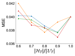
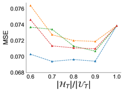
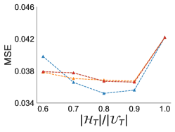
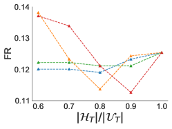
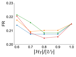
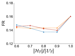
Variation of performance with the fraction of outliers ($\gamma$). Next, we address the research question (2). Figure 1 describes the variation of forecasting performance for different values of $\gamma$ i.e. the pre-specified fraction of outliers, for Club, Verdict and Delhi datasets. In this experiment, $\gamma$ is varied from $0.4$ to $0$, and demarcation methods are used to remove outlier according to a given $\gamma$, followed by parameter estimation over the refined set. As this experiment is mainly intended for showing the effect of the parameter $\gamma$ in our methods on predictive performance, baselines are omitted here. For this experiment, the time span has been fixed to $4$ hours. Here we observe, as we start refining the event set, the prediction performance improves. But if we increase the value of $\gamma$ beyond around 0.4, the performance drops, strongly suggesting an optimum number of outliers present in the training data. If we set a high value of $\gamma$, our methods misclassify many regular events as outliers, while a small value of $\gamma$ ignores their effects.

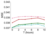
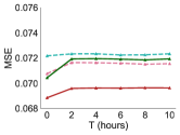
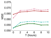
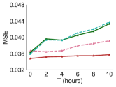
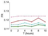
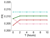
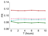
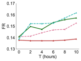
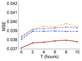
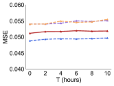
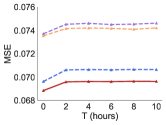
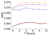
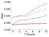
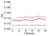
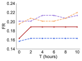
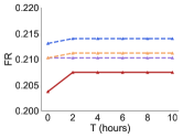
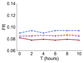
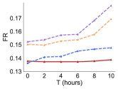
Forecasting performance. Next, we address the research question (3). In particular, we compare the forecasting performance of CherryPick against the baselines. Figure 2 shows the forecasting performance with respect to variation of T, across various representative datasets, for the best performing variant of CherryPick and three best performing baselines (best according to MSE at T = 4 hours), where $\gamma=0.2$. We make the following observations. (I) CherryPick outperforms the baselines for the majority of the cases. (II) Generally, Robust_HT performs better among the baselines. (III) The performance deteriorates as we predict further in the future for all the methods, but the performance stabilizes after a while.

(a)

(b)

(c)

(d)

(e)

(f)

(g) Club

(h) Elections

(i) Verdict

(j) Sports

(k) Delhi

Figure 2. Sentiment prediction performance for five real-world datasets for the best performing variant of CherryPick and three best performing baselines for a fixed $\gamma=0.2$. For each message $m$ in test set, we predict its sentiment value given the history up to T hours before the time of the message. For the T hours, we predict the opinion stream using a sampling algorithm. Mean squared error and failure rate have been reported. We observe CherryPick generally performs better than the baselines on all datasets. Among the baselines, Robust_HT performs comparably with CherryPick on some of the datasets presented here.

Effect of sanitizing test data. Next, we address the research question (4). To that aim, we remove the outliers from the test data by refining entire datasets using variants of CherryPick and then check the prediction performance of the previously computed model (in the experimental settings of Section 5.5) over the refined test set. We compare the prediction error over this sanitized test set with the prediction error over the unrefined test set and report the improvement. We report the prediction error in Table 4 (improvements over the error on the unrefined test set are given in brackets). As observed from the results, for the majority of the cases, refining the test set improves prediction performance, confirming the presence of outliers in the test set which the estimated model will not be able to predict well. Depending on the type and nature of the datasets, the error reduction varies, reaching its highest for Sports and lowest for Club. Among our methods, we observe CherryPick_A and CherryPick_D to perform better than the rest in terms of error reduction. In summary, the effectiveness of CherryPick is more prominent after demarcating the test set.

Datasets	CherryPickA	CherryPickD	CherryPickE	CherryPickT
	MSE
Club	0.038 (1.78%)	0.044 (-16.%)	0.039 (-1.1%)	0.042 (-10.%)
Elections	0.057 (-4.5%)	0.053 (1.48%)	0.051 (6.56%)	0.062 (-19.%)
Verdict	0.068 (2.04%)	0.069 (3.89%)	0.071 (0.51%)	0.074 (-4.4%)
Sports	0.059 (11.9%)	0.042 (24.8%)	0.057 (6.43%)	0.059 (17.1%)
Delhi	0.033 (6.41%)	0.039 (1.15%)	0.0 (100.%)	0.036 (1.41%)
	FR
Club	0.744 (0.29%)	0.140 (-23.%)	0.740 (1.52%)	0.650 (-7.1%)
Elections	0.314 (13.9%)	0.168 (4.59%)	0.252 (28.4%)	0.140 (28.3%)
Verdict	0.685 (0.32%)	0.204 (2.94%)	0.701 (-0.4%)	0.694 (-0.0%)
Sports	0.062 (22.4%)	0.071 (10.9%)	0.051 (20.4%)	0.051 (43.8%)
Delhi	0.474 (19.2%)	0.143 (2.70%)	0.0 (100.%)	0.480 (0.83%)

Table 4. Mean squared error and failure rate of CherryPick_X on all the datasets after demarcating exogenous events from the test set. Error reduction (from error reported on the entire test set) is given in brackets. After demarcating the test set, in the majority of the cases, error reduction is positive, indicating that the error on an unfiltered test set gives an overestimation of the true error.

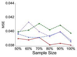
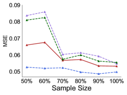
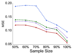
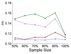
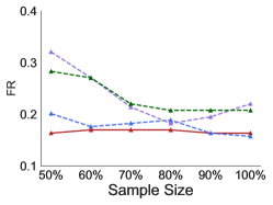
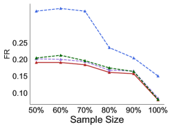
Variation of performance with training set size. Next, we answer the research question (5). Specifically, we evaluate the efficacy of our approaches over varying training set sizes as follows. We use a subset of training data, varying from initial $50\%$ of the total training set to entire $100\%$ for estimating the parameters and test the estimated model on the same test data used in all the experiments, which is the last $10\%$ data of the entire stream of events. Figure 3 summarizes the results over three datasets (Club, Elections and Sports) out of the five real datasets, which reveals the following observations. (I) The performance deteriorates with decreasing training set size for all methods. (II) Our methods generally perform better compared to the baselines over varying training set sizes showing the effectiveness of the demarcation technique. (III) For Elections where the total number of events is quite small compared to the rest, Robust_HT performs better than the variants of CherryPick, indicating hard thresholding to be quite effective for demarcation. (IV) The performance of CherryPick for smaller sample size, relative to its competitors, indicates its stability and robustness.

(a)

(b) Club

(c) Elections

(d) Sports

(e) Club

(f) Elections

(g) Sports

Figure 3. Mean squared error and failure rate on three datasets Club, Elections and Sports for varying size of training data from 50% to 100% of total training data (initial 90% data of entire event collection) for the best performing variant of CherryPick and three best performing baselines. Time span for future prediction T is set to 4 hours and $\gamma$ = 0.2. For all methods, error reduces with increasing training set size. Generally on the entire range, CherryPick performs better than the baselines.

6. Experiments with synthetic data

In this section, we provide a comparative evaluation of the four variants of CherryPick with baselines on a set of three synthetic datasets. To that aim, we address the following research questions here:

1. How do the variants of CherryPick compare in terms of parameter estimation performance across different sizes of training set?

2. How does their predictive performance vary across different levels of noise present in the data?

6.1. Dataset generation

For constructing the synthetic datasets, we have generated the following networks, each with $512$ nodes to use as input to the opinion model (SLANT) (De et al., 2016).

• Kronecker Core-Periphery networks$\colon$ In this Kronecker network, the core is very well connected and there are comparatively fewer nodes in the periphery, sparsely connected with the core (parameter matrix [0.9, 0.5; 0.5, 0.3]).

• Kronecker Random networks: This Kronecker network has been generated using the parameter matrix [0.5, 0.5, 0.5, 0.5].

• Barabasi Albert$\colon$ This is a scale-free network where the network grows iteratively with this preferential attachment property that the more well-connected nodes are more likely to receive new links.

The message stream is generated for each of the networks by simulating the message sampling algorithm proposed in  (De et al., 2016). Each user starts with a latent opinion ($\alpha_{i}$) as well as non-zero opinion influence parameters corresponding to directed edges of the network ($A_{ij}$) sampled from a zero-mean unit variance Gaussian distribution. The rate of intensity ($\mu_{i}$), as well as the intensity influence parameters ($B_{ij}$), are uniformly sampled from the range $[0,1]$. Opinions are sampled from unit variance Gaussian with the mean set as the latent opinion of the user. Using multivariate Hawkes, the events are generated. While generating event times, each event is marked as exogenous with 20% probability and if marked exogenous, it is sampled by a distinct distribution (described later). The kernel used in exponential decay of the opinion ($\omega$) is $1000$ and the kernel for the intensity ($\mu$) is $10$.

6.2. Baselines

We compare our proposed approaches with the same baselines introduced in Section 5.3.

6.3. Evaluation protocol

The evaluation protocol used is the same as in the case of real datasets (Section 5.2).

6.4. Metrics

We measure the performance of our methods and the baselines using the sentiment prediction errors and parameter estimation error of the correspondingly trained endogenous model, depending on corresponding experiment. Specifically, we measure the sentiment prediction error using the mean squared error (MSE) between the actual sentiment value ($m$) and the estimated sentiment value ($\hat{m}$), i.e., $\mathbb{E}[(m-\hat{m})^{2}]$ and the parameter estimation error using the mean squared error (MSE) between the estimated ($\bar{x}$)and true opinion parameters ($x$), i.e., $E[(x-\bar{x})^{2}]$.

6.5. Results

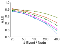
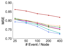
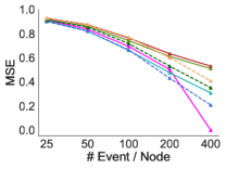
Variation of performance with sample size. Here, we investigate the research question (1). More specifically, to understand the effect of sample size on parameter estimation, we vary the number of events per node from 20 to 400. $20\%$ of the messages are perturbed as exogenous events and they are sampled from a Gaussian distribution with $0.1$ variance and mean sampled separately from a zero-mean-unit-variance Gaussian.

Figure 4 summarizes the results for all variants of CherryPick along with three best performing baselines, which reveals following observations. (I) CherryPick_D and CherryPick_T are able to boost parameter estimation performance across a wide range of training set size, along with showing their robustness and stability with decreasing sample size. Hoewever, CherryPick_A and CherryPick_E are observed to perform poorly over the entire range.(II) Robust_HT shows very comparable performance with best performing variants of CherryPick. We can conclude that CherryPick_D and CherryPick_T are able to identify more useful samples for accurately estimating the parameters compared to CherryPick_A and CherryPick_E. This is because CherryPick_A and CherryPick_E suffer from their weak submodularity property, which renders them disadvantageous due to high SNR of the datasets (40-50 dB) (Chamon and Ribeiro, 2017).

(a)

(b) Barabasi Albert

(c) Kronecker-CP

(d) Kronecker-Random

Figure 4. Mean squared error for parameter estimation on three synthetic datasets against varying training set size. Best performing variants of CherryPick always achieve comparable (if not better) performance with best of the baselines.

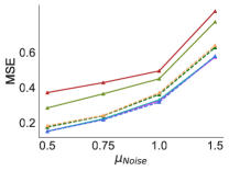
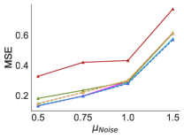
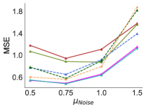
Variation of performance with noise. Here we address research question (2). In particular, to have a better understanding of the effect of noise intensity in the performance of CherryPick, we gradually increase the noise intensity in the message stream in all synthetic datasets and report the sentiment prediction performance of all competing methods. $30000$ events are sampled for each network and $20$% of them are perturbed by adding noises of increasing intensity. The noise is sampled from Gaussian with variance set at $0.05$ and mean varying in the range $[0.5,0.75,1.0,1.5,2.0,2.5]$.

Figure 5 summarizes the results for all variants of CherryPick along with three best performing baselines, where it shows, (i) as prediction error increases sharply with increasing noise for all the methods, CherryPick_D or CherryPick_T outperform or perform comparably with the baselines, (iii) interestingly Robust_HT performs comparably with CherryPick_X in majority of the cases. As we already mentioned, for all the cases, the performance of CherryPick_A or CherryPick_E suffers because their weak submodularity property which renders them ineffective due to high SNR of the corresponding datasets (40-50 dB) (Chamon and Ribeiro, 2017).

(a)

(b) Barabasi Albert

(c) Kronecker-CP

(d) Kronecker-Random

Figure 5. Sentiment prediction error in terms of mean squared error on three synthetic datasets against varying intensity of noise. Best performing variants of CherryPick degrade gracefully in comparison with the baselines for most of the cases.

7. Conclusion

The principal contribution of this paper lies in emphatically establishing the dual nature of message flow over online social network: injection of exogenous opinions and influence-based dynamics, internal to the network. The realization helps us to propose CherryPick_X, a set of novel learning methodologies to demarcate endogenous and exogenous opinions and illustrate their utility by analyzing their performance from an opinion modeling perspective. In CherryPick_X, to this aim, we formulated the message classification problem as a submodular optimization task in the set of messages, which we solved using an efficient greedy algorithm. Our proposed techniques are very easy to implement, extremely scalable (particularly CherryPick_A and CherryPick_T) and quite effective in serving their purpose, showing their superiority over the baselines which were designed by robust regression literature. Finally, on various real datasets crawled from Twitter as well as synthetic datasets, we showed that our proposals consistently outperform various outlier removal algorithms in terms of predictive performance. The superior performance is even more remarkable considering the fact that we train our system on smaller (but relevant) amounts of data.

Appendix A Proofs of results

A.1. Proof of Lemma 4.1

For any $u\in\mathcal{V}$, define $\bm{\theta}_{u}=[\bm{A}_{u};\alpha_{u}]$. We observe the loss (Eq. 10) associated with only user $u$ is a regularized least squares loss, i.e.,

(29) $$\hat{\bm{\theta}}_{u}=\underset{\bm{\theta}_{u}}{\text{min}} \sum_{e_{i}\in\mathcal{H}_{T}}\sigma^{-2}\Big{(}m^{*}_{u}(t_{i})-\bm{\phi}_{i}^{uT}\bm{\theta}_{u}\Big{)}^{2}+c||\bm{\theta}_{u}||_{2}^{2},$$

$$\hat{\bm{\theta}}_{u} =\Big{(}c\bm{I}+\sigma^{-2}\sum_{e_{i}\in\mathcal{H}_{T}}\bm{\phi}^{u}_{i}\bm{\phi}^{uT}_{i}\Big{)}^{-1}\sigma^{-2}\sum_{e_{i}\in\mathcal{H}_{T}}m_{u}(t_{i})\bm{\phi}^{u}_{i}$$

$$=\Big{(}c\bm{I}+\sigma^{-2}\sum_{e_{i}\in\mathcal{H}_{T}}\bm{\phi}^{u}_{i}\bm{\phi}^{uT}_{i}\Big{)}^{-1}\sigma^{-2}\sum_{e_{i}\in\mathcal{H}_{T}}\bm{\phi}^{u}_{i}\bm{\phi}^{uT}_{i}\bm{\theta}_{u}+\Big{(}c\bm{I}+\sigma^{-2}\sum_{e_{i}\in\mathcal{H}_{T}}\bm{\phi}^{u}_{i}\bm{\phi}^{uT}_{i}\Big{)}^{-1}\sum_{e_{i}\in\mathcal{H}_{T}}\bm{\phi}^{u}_{i}\frac{\epsilon(t_{i})}{\sigma^{2}}$$

The equality follows from the fact that,  $m_{u}(t_{i})=\bm{\phi}^{uT}_{i}\bm{\theta}_{u}+\epsilon(t_{i})$

$$\hat{\bm{\theta}}_{u}-\bm{\theta}_{u} =-c\Big{(}c\bm{I}+\sigma^{-2}\sum_{e_{i}\in\mathcal{H}_{T}}\bm{\phi}^{u}_{i}\bm{\phi}^{uT}_{i}\Big{)}^{-1}\bm{\theta}_{u}+\Big{(}c\bm{I}+\sigma^{-2}\sum_{e_{i}\in\mathcal{H}_{T}}\bm{\phi}^{u}_{i}\bm{\phi}^{uT}_{i}\Big{)}^{-1}\sum_{e_{i}\in\mathcal{H}_{T}}\bm{\phi}^{u}_{i}\frac{\epsilon(t_{i})}{\sigma^{2}}$$

Then the covariance product is given in the following:

$$\mathbb{E}(\hat{\bm{\theta}}_{u}-\bm{\theta}_{u})(\hat{\bm{\theta}}_{u}-\bm{\theta}_{u})^{T} =c^{2}\Big{(}c\bm{I}+\sigma^{-2}\sum_{e_{i}\in\mathcal{H}_{T}}\bm{\phi}^{u}_{i}\bm{\phi}^{uT}_{i}\Big{)}^{-1}\mathbb{E}[\bm{\theta}_{u}\bm{\theta}^{T}_{u}]\Big{(}c\bm{I}+\sigma^{-2}\sum_{e_{i}\in\mathcal{H}_{T}}\bm{\phi}^{u}_{i}\bm{\phi}^{uT}_{i}\Big{)}^{-1}$$

$$+\Big{(}c\bm{I}+\sigma^{-2}\sum_{e_{i}\in\mathcal{H}_{T}}\bm{\phi}^{u}_{i}\bm{\phi}^{uT}_{i}\Big{)}^{-1}\sum_{e_{i}\in\mathcal{H}_{T}}\bm{\phi}^{u}_{i}\bm{\phi}^{uT}_{i}\frac{\mathbb{E}(\epsilon^{2}(t_{i}))}{\sigma^{4}}\Big{(}c\bm{I}+\sigma^{-2}\sum_{e_{i}\in\mathcal{H}_{T}}\bm{\phi}^{u}_{i}\bm{\phi}^{uT}_{i}\Big{)}^{-1}$$

Note that, from the regularizer we have, $\bm{\theta}_{u}\sim\mathcal{N}(0,\bm{I}/c)$. Furthermore $\mathbb{E}(\epsilon^{2}(t_{i}))=\sigma^{2}$. Using simple algebraic calculation, we have the value for $\bm{\Sigma}(\mathcal{H}_{T})$.

A.2. Proof of Theorem 4.3

(i) Monotonicity of $f_{X}$ : To prove monotonicity, we need to show, $f_{X}(\mathcal{H}_{T}\cup\{e_{k}\})-f_{X}(\mathcal{H}_{T})\geq 0$. Recall that the set of users posting the messages is denoted by $\mathcal{V}$. Assume the user $u$ has posted the event $e_{k}=\{u_{k},m_{k},t_{k}\}$, i.e. $u_{k}=u$. We define an auxiliary function of $p\in[0,1]$:

$$g(p):=\sum_{u\in\mathcal{V}}\mathop{\mathrm{tr}}\log\Big{(}c\bm{I}+\sigma^{-2}\sum_{e_{i}\in\mathcal{H}_{T}}\bm{\phi}^{u}_{i}\bm{\phi}_{i}^{uT}+p\sigma^{-2}\bm{\phi}^{u}_{k}\bm{\phi}_{k}^{uT}\Big{)}.\vspace*{-0.2cm}$$

Monotonicity of $f_{X}$ in $\mathcal{H}_{T}$ is equivalent to the condition: $g(1)\geq g(0)$ that can be shown by proving $\frac{d}{dp}g(p)\geq 0$. For compactness, we define $\bm{G}_{u}=\Big{(}c\bm{I}+\sigma^{-2}\sum_{e_{i}\in\mathcal{H}_{T}}\bm{\phi}^{u}_{i}\bm{\phi}_{i}^{uT}\Big{)}$. Now we can show that:

$$\frac{d}{dp}g(p) =\sum_{u\in\mathcal{V}}\mathop{\mathrm{tr}}\frac{d}{dp}\log(\bm{G}_{u}+p\bm{\phi}^{u}_{k}\bm{\phi}_{k}^{uT})$$

$$=\sum_{u\in\mathcal{V}}\mathop{\mathrm{tr}}\frac{d}{dp}\Big{[}\log(\bm{G}_{u}+p\bm{\phi}^{u}_{k}\bm{\phi}_{k}^{uT})-\log\bm{G}_{u}\Big{]}$$

$$=\sum_{u\in\mathcal{V}}\mathop{\mathrm{tr}}\big{[}(\bm{I}+p\bm{\phi}^{u}_{k}\bm{\phi}_{k}^{uT}\bm{G}_{u}^{-1})^{-1}\bm{\phi}^{u}_{k}\bm{\phi}_{k}^{uT}\bm{G}_{u}^{-1}\big{]}$$

$$=\sum_{u\in\mathcal{V}}\mathop{\mathrm{tr}}\bm{\phi}_{k}^{uT}\bm{G}_{u}^{-1}(\bm{I}+p\bm{\phi}^{u}_{k}\bm{\phi}_{k}^{uT}\bm{G}_{u}^{-1})^{-1}\bm{\phi}^{u}_{k}$$

(30) $$=\sum_{u\in\mathcal{V}}\sigma^{-2}\bm{\phi}_{k}^{uT}(\bm{G}_{u}+p\bm{\phi}^{u}_{k}\bm{\phi}_{k}^{uT})^{-1}\bm{\phi}_{k}^{u}\geq 0$$

Hence $f_{X}$ is monotone in $\mathcal{H}_{T}$ $\forall X\in\{A,D,E,T\}$.

(ii) Weak submodularity of $f_{A}$ and $f_{E}$ : Since $f_{A}$ and $f_{E}$ are linear and monotone as proved above, their weak submodularity follows from the weak submodularity of the A and E optimality criteria which has been proved in (Bian et al., 2017; Chamon and Ribeiro, 2017; Hashemi et al., 2018) for linear and monotone observation models.

(iii) Submodularity of $f_{D}$ : Since $f_{D}$ is linear and monotone as proved above, its submodularity follows from the submodularity of the D optimality criterion which has been proved in (Krause et al., 2008; Shamaiah et al., 2010) for linear and monotone observation models.

(iv) Modularity of $f_{T}$ : Since $f_{T}$ is linear and monotone as proved above, its modularity follows from the modularity of the T optimality criterion which has been proved in (Krause et al., 2008; Summers et al., 2015) for linear and monotone observation models.

Appendix B Additional Results

Datasets	CherryPickA-Gr	CherryPickA-Fast	CherryPickD-Gr	CherryPickD-Fast
	Mean squared error: $\mathbb{E}(m-\hat{m})^{2}$
Club	0.038	0.039	0.037	0.037
Elections	0.054	0.055	0.053	0.051
Verdict	0.069	0.071	0.071	0.072
Sports	0.066	0.067	0.056	0.057
Delhi	0.035	0.036	0.039	0.039
	Failure Rate: $\mathbb{P}(\text{sign}(m)\neq\mathbb{P}(\text{sign}(\hat{m}))$
Club	0.120	0.124	0.113	0.116
Elections	0.169	0.176	0.176	0.182
Verdict	0.207	0.204	0.210	0.213
Sports	0.114	0.091	0.079	0.087
Delhi	0.137	0.144	0.147	0.152

Table 5. Comparative performance evaluation of CherryPick_A-Fast and CherryPick_D-Fast with CherryPick_A-Gr and CherryPick_D-Gr for five real-world datasets for fixed $\gamma=0.2$ and T =4 hours. For each message $m$ in test set, we predict its sentiment value given the history up to T =4 hours before the time of the message. For the T hours, we predict the opinion stream using a sampling algorithm. Mean squared error and failure rate have been reported. We observe that, in general, greedy variants outperform adaptive variants by small margin.

For the experimental results, we apply standard greedy for maximizing $f_{A}$ and $f_{D}$ (see Section 5). As we have mentioned earlier, there exist fast adaptive techniques as alternative to greedy for both maximization of $f_{D}$ as well as $f_{A}$. In this section, we repeat our primary experiments with fast adaptive techniques for CherryPick_A and CherryPick_D and compare them with their greedy alternatives. For maximizing $f_{D}$, we use Fast-Full, a fast adaptive algorithm proposed in (Breuer et al., 2020). We refer to this method as CherryPick_D-Fast. For maximizing $f_{A}$, we adopt DASH, a fast adaptive technique proposed by (Qian and Singer, 2019), which we refer to as CherryPick_A-Fast. From now onwards, we refer to greedy techniques for $f_{A}$ and $f_{D}$ as CherryPick_A-Gr and CherryPick_D-Gr respectively. We present their detailed comparative evaluation in our primary experiments on real datasets below.

Comparative analysis. Here we compare the predictive performance of CherryPick_A-Fast and CherryPick_D-Fast with CherryPick_A-Gr and CherryPick_D-Gr. We fix the fraction of endogenous chosen to $0.8$ and prediction time to 4 hours. We follow the same setup as in the corresponding experiment in Section 5. Table 5 summarizes the results. In aggregate, we observe the trade-off that fast adaptive techniques either perform comparably with the greedy methods or standard greedy algorithms outperform adaptive methods by a small margin at the cost of speeding up the demarcation process.

(a)

(b) Club

(c) Verdict

(d) Delhi

(e) Club

(f) Verdict

(g) Delhi

Figure 6. Performance variation with size of endogenous subset for Club, Verdict and Delhi datasets where the size of endogenous subset is varied from 60% to 100%. Timespan T has been set to 4 hours. Mean squared error and failure rate have been reported. Adaptive variants display almost identical behavior with greedy variants.

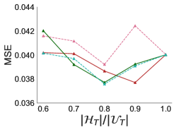
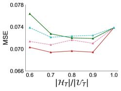
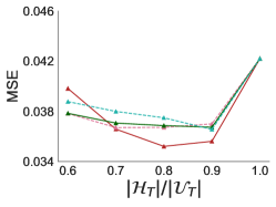
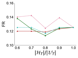
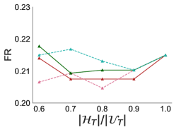
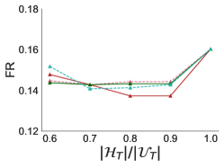
Variation of performance with the fraction of outliers ($\gamma$). Figure 6 compares greedy and adaptive variants of CherryPick_A and CherryPick_D by observing the variation of forecasting performance for different values of $\gamma$ i.e. the pre-specified fraction of outliers, for Club, Verdict, and Delhi datasets. In this experiment, $\gamma$ is varied from $0.4$ to $0$, and the timespan has been fixed to $4$ hours. Here we observe both CherryPick_A-Fast and CherryPick_D-Fast perform very similar to CherryPick_A-Gr and CherryPick_D-Gr respectively. Moreover, CherryPick_A-Fast and CherryPick_D-Fast preserve the same behavioral pattern as their greedy counterpart i.e. both performing best for a fixed value of $\gamma$, with performance drop at both ends.

Forecasting performance. Finally, we compare the forecasting performance of CherryPick_A-Fast and CherryPick_D-Fast with their greedy counterparts with respect to variation of T, fixing $\gamma=0.2$. Figure 7 summarizes the results, where we make following observations. (I) Generally, both CherryPick_A-Fast and CherryPick_D-Fast are outperformed by their greedy counterparts with very low margin as T increases. (II) CherryPick_A-Fast and CherryPick_D-Fast display a similar pattern of performance drop with higher T with small deviations from the greedy counterparts.

(a)

(b)

(c)

(d)

(e)

(f) Club

(g) Verdict

(h) Sports

(i) Delhi

Figure 7. Forecasting performance for greedy and adaptive variants of CherryPick_A and CherryPick_D for a fixed $\gamma=0.2$ for four major real datasets. For each message $m$ in the test set, we predict its sentiment value given the history up to T hours before the time of the message. For the T hours, we predict the opinion stream using a sampling algorithm. Mean squared error and failure rate have been reported. We observe almost identical behavior of greedy and adaptive variants, with adaptive methods outperformed by greedy methods with negligible margin.

References

- (1)
- Altafini and Lini (2015) Claudio Altafini and Gabriele Lini. 2015. Predictable dynamics of opinion forming for networks with antagonistic interactions. IEEE Trans. Automat. Control 60, 2 (2015), 342–357.
- Anagnostopoulos et al. (2008) Aris Anagnostopoulos, Ravi Kumar, and Mohammad Mahdian. 2008. Influence and correlation in social networks. In Proceedings of the 14th ACM SIGKDD international conference on Knowledge discovery and data mining. ACM, 7–15.
- Aral and Walker (2011) Sinan Aral and Dylan Walker. 2011. Creating social contagion through viral product design: A randomized trial of peer influence in networks. Management science 57, 9 (2011), 1623–1639.
- Bakshy et al. (2012a) Eytan Bakshy, Dean Eckles, Rong Yan, and Itamar Rosenn. 2012a. Social influence in social advertising: evidence from field experiments. In Proceedings of the 13th ACM conference on electronic commerce. 146–161.
- Bakshy et al. (2012b) Eytan Bakshy, Itamar Rosenn, Cameron Marlow, and Lada Adamic. 2012b. The role of social networks in information diffusion. In Proceedings of the 21st international conference on World Wide Web. 519–528.
- Bhatia et al. (2015) Kush Bhatia, Prateek Jain, and Purushottam Kar. 2015. Robust regression via hard thresholding. In Advances in Neural Information Processing Systems. 721–729.
- Bian et al. (2017) Andrew An Bian, Joachim M Buhmann, Andreas Krause, and Sebastian Tschiatschek. 2017. Guarantees for greedy maximization of non-submodular functions with applications. arXiv preprint arXiv:1703.02100 (2017).
- Blondel et al. (2009) Vincent D Blondel, Julien M Hendrickx, and John N Tsitsiklis. 2009. On Krause’s multi-agent consensus model with state-dependent connectivity. IEEE transactions on Automatic Control 54, 11 (2009), 2586–2597.
- Breuer et al. (2020) Adam Breuer, Eric Balkanski, and Yaron Singer. 2020. The FAST algorithm for submodular maximization. In International Conference on Machine Learning. PMLR, 1134–1143.
- Castelló et al. (2006) Xavier Castelló, Víctor M Eguíluz, and Maxi San Miguel. 2006. Ordering dynamics with two non-excluding options: bilingualism in language competition. New Journal of Physics 8, 12 (2006), 308.
- Centola (2010) Damon Centola. 2010. The spread of behavior in an online social network experiment. science 329, 5996 (2010), 1194–1197.
- Chaloner and Verdinelli (1995) Kathryn Chaloner and Isabella Verdinelli. 1995. Bayesian experimental design: A review. Statist. Sci. (1995), 273–304.
- Chamon and Ribeiro (2017) Luiz Chamon and Alejandro Ribeiro. 2017. Approximate supermodularity bounds for experimental design. In Advances in Neural Information Processing Systems. 5403–5412.
- Clifford and Sudbury (1973) P. Clifford and A. Sudbury. 1973. A model for spatial conflict. Biometrika 60, 3 (1973), 581–588.
- Das et al. (2014) A. Das, S. Gollapudi, and K. Munagala. 2014. Modeling opinion dynamics in social networks. In WSDM.
- De et al. (2014) A. De, S. Bhattacharya, P. Bhattacharya, N. Ganguly, and S. Chakrabarti. 2014. Learning a Linear Influence Model from Transient Opinion Dynamics. In CIKM.
- De et al. (2018) Abir De, Sourangshu Bhattacharya, and Niloy Ganguly. 2018. Demarcating endogenous and exogenous opinion diffusion process on social networks. In Proceedings of the 2018 World Wide Web Conference. 549–558.
- De et al. (2016) Abir De, Isabel Valera, Niloy Ganguly, Sourangshu Bhattacharya, and Manuel Gomez Rodriguez. 2016. Learning and Forecasting Opinion Dynamics in Social Networks. In NIPS.
- Deffuant et al. (2000) Guillaume Deffuant, David Neau, Frederic Amblard, and Gérard Weisbuch. 2000. Mixing beliefs among interacting agents. Advances in Complex Systems 3, 01n04 (2000), 87–98.
- DeGroot (1974) M. H. DeGroot. 1974. Reaching a consensus. J. Amer. Statist. Assoc. 69, 345 (1974), 118–121.
- Dittmer (2001) Jan Christian Dittmer. 2001. Consensus formation under bounded confidence. Nonlinear Analysis: Theory, Methods & Applications 47, 7 (2001), 4615–4621.
- Douven and Riegler (2009) Igor Douven and Alexander Riegler. 2009. Extending the Hegselmann–Krause Model I. Logic Journal of IGPL 18, 2 (2009), 323–335.
- Durrett and Levin (1996) Rick Durrett and Simon Levin. 1996. Spatial models for species-area curves. Journal of Theoretical Biology 179, 2 (1996), 119–127.
- Etesami and Başar (2015) Seyed Rasoul Etesami and Tamer Başar. 2015. Game-theoretic analysis of the Hegselmann-Krause model for opinion dynamics in finite dimensions. IEEE Trans. Automat. Control 60, 7 (2015), 1886–1897.
- Farajtabar et al. (2015) M. Farajtabar, Y. Wang, M. Gomez-Rodriguez, S. Li, H. Zha, and L. Song. 2015. COEVOLVE: A Joint Point Process Model for Information Diffusion and Network Co-evolution. In NIPS ’15: Advances in Neural Information Processing Systems.
- Friedkin (2015) Noah E Friedkin. 2015. The problem of social control and coordination of complex systems in sociology: A look at the community cleavage problem. IEEE Control Systems 35, 3 (2015), 40–51.
- Friggeri et al. (2014) A. Friggeri, L. Adamic, D. Eckles, and J. Cheng. 2014. Rumor Cascades. In ICWSM.
- Grabowicz et al. (2016) Przemyslaw A Grabowicz, Niloy Ganguly, and Krishna P Gummadi. 2016. Distinguishing between Topical and Non-Topical Information Diffusion Mechanisms in Social Media.. In ICWSM. 151–160.
- Greenhalgh et al. (2004) Trisha Greenhalgh, Glenn Robert, Fraser Macfarlane, Paul Bate, and Olivia Kyriakidou. 2004. Diffusion of innovations in service organizations: systematic review and recommendations. The Milbank Quarterly 82, 4 (2004), 581–629.
- Gupta et al. (2021) V. Gupta, A. De, S. Bhattacharya, and S. Bedathur. 2021. Learning Temporal Point Processes with Intermittent Observations. In AISTATS.
- Hannak et al. (2012) Aniko Hannak, Eric Anderson, Lisa Feldman Barrett, Sune Lehmann, Alan Mislove, and Mirek Riedewald. 2012. Tweetin’in the Rain: Exploring Societal-Scale Effects of Weather on Mood.. In ICWSM.
- Hashemi et al. (2018) Abolfazl Hashemi, Mahsa Ghasemi, Haris Vikalo, and Ufuk Topcu. 2018. A randomized greedy algorithm for near-optimal sensor scheduling in large-scale sensor networks. In 2018 Annual American Control Conference (ACC). IEEE, 1027–1032.
- Hashemi et al. (2019) Abolfazl Hashemi, Mahsa Ghasemi, Haris Vikalo, and Ufuk Topcu. 2019. Submodular observation selection and information gathering for quadratic models. arXiv preprint arXiv:1905.09919 (2019).
- Hegselmann and Krause (2002) R. Hegselmann and U. Krause. 2002. Opinion dynamics and bounded confidence models, analysis, and simulation. Journal of Artificial Societies and Social Simulation 5, 3 (2002).
- Holme and Newman (2006) P. Holme and M. E. Newman. 2006. Nonequilibrium phase transition in the coevolution of networks and opinions. Physical Review E 74, 5 (2006), 056108.
- Hosseinia and Mukherjee (2017) Marjan Hosseinia and Arjun Mukherjee. 2017. Detecting Sockpuppets in Deceptive Opinion Spam. arXiv preprint arXiv:1703.03149 (2017).
- KC and Mukherjee (2016) Santosh KC and Arjun Mukherjee. 2016. On the temporal dynamics of opinion spamming: Case studies on yelp. In Proceedings of the 25th International Conference on World Wide Web. International World Wide Web Conferences Steering Committee, 369–379.
- Krause and Golovin (2014) Andreas Krause and Daniel Golovin. 2014. Submodular function maximization.
- Krause et al. (2008) Andreas Krause, Ajit Singh, and Carlos Guestrin. 2008. Near-optimal sensor placements in Gaussian processes: Theory, efficient algorithms and empirical studies. Journal of Machine Learning Research 9, Feb (2008), 235–284.
- Krause (2000) Ulrich Krause. 2000. A discrete nonlinear and non-autonomous model of consensus formation. Communications in difference equations (2000), 227–236.
- Li et al. (2015) Huayi Li, Zhiyuan Chen, Arjun Mukherjee, Bing Liu, and Jidong Shao. 2015. Analyzing and Detecting Opinion Spam on a Large-scale Dataset via Temporal and Spatial Patterns.. In ICWSM. 634–637.
- Li et al. (2017) Huayi Li, Geli Fei, Shuai Wang, Bing Liu, Weixiang Shao, Arjun Mukherjee, and Jidong Shao. 2017. Bimodal distribution and co-bursting in review spam detection. In Proceedings of the 26th International Conference on World Wide Web. International World Wide Web Conferences Steering Committee, 1063–1072.
- Liniger (2009) T.J. Liniger. 2009. Multivariate Hawkes Processes. Ph.D. Dissertation. ETHZ.
- Liu (2012) Bing Liu. 2012. Sentiment analysis and opinion mining. Synthesis lectures on human language technologies 5, 1 (2012), 1–167.
- Medeiros et al. (2006) Nazareno GF Medeiros, Ana TC Silva, and FG Brady Moreira. 2006. Domain motion in the voter model with noise. Physical Review E 73, 4 (2006), 046120.
- Mobilia (2003) Mauro Mobilia. 2003. Does a single zealot affect an infinite group of voters? Physical review letters 91, 2 (2003), 028701.
- Mor et al. (2011) Irinel-Constantin Mor, Antoine Girard, et al. 2011. Opinion dynamics with decaying confidence: Application to community detection in graphs. IEEE Trans. Automat. Control 56, 8 (2011), 1862–1873.
- Morărescu et al. (2016) Irinel-Constantin Morărescu, Samuel Martin, Antoine Girard, and Aurélie Muller-Gueudin. 2016. Coordination in networks of linear impulsive agents. IEEE Trans. Automat. Control 61, 9 (2016), 2402–2415.
- Myers et al. (2012) Seth A Myers, Chenguang Zhu, and Jure Leskovec. 2012. Information diffusion and external influence in networks. In Proceedings of the 18th ACM SIGKDD international conference on Knowledge discovery and data mining. ACM, 33–41.
- Nasrabadi et al. (2011) Nasser M Nasrabadi, Trac D Tran, and Nam Nguyen. 2011. Robust lasso with missing and grossly corrupted observations. In Advances in Neural Information Processing Systems. 1881–1889.
- Nemhauser et al. (1978a) George L Nemhauser, Laurence A Wolsey, and Marshall L Fisher. 1978a. An analysis of approximations for maximizing submodular set functions—I. Mathematical Programming 14, 1 (1978), 265–294.
- Nemhauser et al. (1978b) George L Nemhauser, Laurence A Wolsey, and Marshall L Fisher. 1978b. An analysis of approximations for maximizing submodular set functions—I. Mathematical programming 14, 1 (1978), 265–294.
- Pang and Lee (2008) B. Pang and L. Lee. 2008. Opinion mining and sentiment analysis. Foundations and trends in information retrieval 2, 1-2 (2008), 1–135.
- Pennebaker et al. (2001) James W Pennebaker, Martha E Francis, and Roger J Booth. 2001. Linguistic inquiry and word count: LIWC 2001. Mahway: Lawrence Erlbaum Associates 71, 2001 (2001), 2001.
- Qian and Singer (2019) Sharon Qian and Yaron Singer. 2019. Fast parallel algorithms for statistical subset selection problems. In Advances in Neural Information Processing Systems. 5072–5081.
- Schweitzer and Behera (2009) Frank Schweitzer and Laxmidhar Behera. 2009. Nonlinear voter models: the transition from invasion to coexistence. The European Physical Journal B-Condensed Matter and Complex Systems 67, 3 (2009), 301–318.
- Shamaiah et al. (2010) Manohar Shamaiah, Siddhartha Banerjee, and Haris Vikalo. 2010. Greedy sensor selection: Leveraging submodularity. In 49th IEEE conference on decision and control (CDC). IEEE, 2572–2577.
- Summers et al. (2015) Tyler H Summers, Fabrizio L Cortesi, and John Lygeros. 2015. On submodularity and controllability in complex dynamical networks. IEEE Transactions on Control of Network Systems 3, 1 (2015), 91–101.
- Tsakonas et al. (2014) Efthymios Tsakonas, Joakim Jaldén, Nicholas D Sidiropoulos, and Björn Ottersten. 2014. Convergence of the Huber regression M-estimate in the presence of dense outliers. IEEE Signal Processing Letters 21, 10 (2014), 1211–1214.
- Valente (1996) Thomas W Valente. 1996. Social network thresholds in the diffusion of innovations. Social networks 18, 1 (1996), 69–89.
- Vazquez and Eguíluz (2008) Federico Vazquez and Víctor M Eguíluz. 2008. Analytical solution of the voter model on uncorrelated networks. New Journal of Physics 10, 6 (2008), 063011.
- Vazquez et al. (2003) Federico Vazquez, Paul L Krapivsky, and Sidney Redner. 2003. Constrained opinion dynamics: Freezing and slow evolution. Journal of Physics A: Mathematical and General 36, 3 (2003), L61.
- Wang et al. (2017) Yichen Wang, Grady Williams, Evangelos Theodorou, and Le Song. 2017. Variational Policy for Guiding Point Processes. arXiv preprint arXiv:1701.08585 (2017).
- Weisbuch et al. (2002) Gérard Weisbuch, Guillaume Deffuant, Frédéric Amblard, and Jean-Pierre Nadal. 2002. Meet, discuss, and segregate! Complexity 7, 3 (2002), 55–63.
- Williamson and Shmoys (2011) David P Williamson and David B Shmoys. 2011. The design of approximation algorithms. Cambridge university press.
- Yildiz et al. (2013) E. Yildiz, A. Ozdaglar, D. Acemoglu, A. Saberi, and A. Scaglione. 2013. Binary opinion dynamics with stubborn agents. ACM Transactions on Economics and Computation 1, 4 (2013), 19.
- Yildiz et al. (2010) M. E. Yildiz, R. Pagliari, A. Ozdaglar, and A. Scaglione. 2010. Voting models in random networks. In Information Theory and Applications Workshop. 1–7.
- Zarezade et al. (2017) Ali Zarezade, Abir De, Hamid Rabiee, and Manuel Gomez-Rodriguez. 2017. Cheshire: An Online Algorithm for Activity Maximization in Social Networks. In arXiv preprint arXiv:1703.02059.