Emotion Transfer Using Vector-Valued Infinite Task Learning
Abstract
Style transfer is a significant problem of machine learning with numerous successful applications. In this work, we present a novel style transfer framework building upon infinite task learning and vector-valued reproducing kernel Hilbert spaces. We instantiate the idea in emotion transfer where the goal is to transform facial images to different target emotions. The proposed approach provides a principled way to gain explicit control over the continuous style space. We demonstrate the efficiency of the technique on popular facial emotion benchmarks, achieving low reconstruction cost and high emotion classification accuracy.
1 Introduction
Recent years have witnessed an increasing attention around style transfer problems (Gatys et al., 2016; Wynen et al., 2018; Jing et al., 2020) in machine learning. In a nutshell, style transfer refers to the transformation of an object according to a target style. It has found numerous applications in computer vision (Ulyanov et al., 2016; Choi et al., 2018; Puy and Pérez, 2019; Yao et al., 2020), natural language processing (Fu et al., 2018) as well as audio signal processing (Grinstein et al., 2018) where objects at hand are contents in which style is inherently part of their perception. Style transfer is one of the key components of data augmentation (Mikołajczyk and Grochowski, 2018) as a means to artificially generate meaningful additional data for the training of deep neural networks. Besides, it has also been shown to be useful for counterbalancing bias in data by producing stylized contents with a well-chosen style (see for instance Geirhos et al. (2019)) in image recognition. More broadly, style transfer fits into the wide paradigm of parametric modeling, where a system, a process or a signal can be controlled by its parameter value. Adopting this perspective, style transfer-like applications can also be found in digital twinning (Tao et al., 2019; Barricelli et al., 2019; Lim et al., 2020), a field of growing interest in health and industry.
In this work, we propose a novel principled approach for style transfer, exemplified in the context of emotion transfer of face images. Given a set of emotions, classical emotion transfer refers to the task of transforming face images according to these target emotions. The pioneering works in emotion transfer include that of Blanz and Vetter (1999) who proposed a morphable 3D face model whose parameters could be modified for facial attribute editing. Susskind et al. (2008) designed a deep belief net for facial expression generation using action unit (AU) annotations.
More recently, extensions of generative adversarial networks (GANs, Goodfellow et al. 2014) have proven to be particularly powerful for tackling image-to-image translation problems (Zhu et al., 2017). Several works have addressed emotion transfer for facial images by conditioning GANs on a variety of guiding information ranging from discrete emotion labels to photos and videos. In particular, StarGAN (Choi et al., 2018) is conditioned on discrete expression labels for face synthesis. ExprGAN (Ding et al., 2018) proposes synthesis with the ability to control expression intensity through a controller module conditioned on discrete labels. Other GAN-based approaches make use of additional information such as AU labels (Pumarola et al., 2018), target landmarks (Qiao et al., 2018), fiducial points (Song et al., 2018) and photos/videos (Geng et al., 2018). While GANs have achieved high quality image synthesis, they come with some pitfalls: they are particularly difficult to train and require large amounts of training data.
In this paper, unlike previous approaches, we adopt a functional point of view: given some person, we assume that the full range of the emotional faces can be modelled as a continuous function from emotions to images. This view exploits the geometry of the representation of emotions (Russell, 1980), assuming that one can pass a facial image “continuously” from one emotion to an other. We then propose to address the problem of emotion transfer by learning an image-to-function model able to predict for a given facial input image represented by its landmarks (Tautkute et al., 2018), the continuous function that maps an emotion to the image transformed by this emotion.
This function-valued regression approach relies on a technique recently introduced by Brault et al. (2019) called infinite task learning (ITL). ITL enlarges the scope of multi-task learning (Evgeniou and Pontil, 2004; Evgeniou et al., 2005) by learning to solve simultaneously a set of tasks parametrized by a continuous parameter. While strongly linked to other parametric learning methods such the one proposed by Takeuchi et al. (2006), the approach differs from previous works by leveraging the use of operator-valued kernels and vector-valued reproducing kernel Hilbert spaces (vRKHS; Pedrick 1957; Micchelli and Pontil 2005; Carmeli et al. 2006). vRKHSs have proven to be relevant in solving supervised learning tasks such as multiple quantile regression (Sangnier et al., 2016) or unsupervised problems like anomaly detection (Schölkopf et al., 2001). A common property of these works is that the output to be predicted is a real-valued function of a real parameter.
To solve the emotion transfer problem, we present an extension of ITL, vector ITL (or shortly vITL) which involves functional outputs with vectorial representation of the faces and the emotions, showing that the approach is still easily controllable by the choice of appropriate kernels guaranteeing continuity and smoothness. In particular, the functional point of view by the inherent regularization induced by the kernel makes the approach suitable even for limited and partially observed emotional images. We demonstrate the efficiency of the vITL approach in a series of numerical experiments showing that it can achieve state-of-the-art performance on two benchmark datasets.
The paper is structured as follows. We formulate the problem and introduce the vITL framework in Section 2. Section 3 is dedicated to the underlying optimization problem. Numerical experiments conducted on two benchmarks of the domain are presented in Section 4. Discussion and future work conclude the paper in Section 5. Proofs of auxiliary lemmas are collected in Section 6.
2 Problem Formulation
In this section we define our problem. Our aim is to design a system capable of transferring emotions: having access to the face image of a given person our goal is to convert his/her face to a specified target emotion. In other words, the system should implement a mapping of the form
| (1) |
In order to tackle this task, one requires a representation of the emotions, and similarly that of the faces. The classical categorical description of emotions deals with the classes ‘happy’, ‘sad’, ‘angry’, ‘surprised’, ‘disgusted’, ‘fearful’. The valence-arousal model (Russell, 1980) embeds these categories into the -dimensional space. The resulting representation of the emotions are points , each coordinate of these vectors encoding the valence (pleasure to displeasure) and arousal (high to low) associated to the emotions. This is the emotion representation we use while noting that there are alternative encodings in higher dimension (, ; Vemulapalli and Agarwala 2019) to which the presented framework can be naturally adapted. Throughout this work faces are represented by landmark points. Landmarks have been proved to be a useful representation in facial recognition (Saragih et al., 2009; Scherhag et al., 2018; Zhang et al., 2015), 3D facial reconstruction and sentiment analysis. Tautkute et al. (2018) have shown that emotions can be accurately recognized by detecting changes in the localization of the landmarks. Given number of landmarks on the face, this means a description .
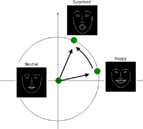
The resulting mapping (1) is illustrated in Fig. 1: starting from a neutral face and the target happy one can traverse to the happy face; from the happy face, given the target emotion surprise one can get to the surprised face.
In an ideal world, for each person, one would have access to a trajectory mapping each emotion to the corresponding landmark locations ; this function can be taken for instance to be the element of , the space of -valued square-integrable function w.r.t. to a measure . The probability measure allows capturing the frequency of the individual emotions. In practice, one has realizations , each corresponds to a single person possible appearing multiple times. The trajectories are observable at finite many emotions where .111To keep the notation simple, we assume that is the same for all the -s. In order to capture relation (1) one can rely on a hypothesis space with elements
| (2) |
The value represents the landmark prediction from face and target emotion .
We consider two tasks for emotion transfer:
-
•
Single emotional input: In the first problem, the assumption is that all the faces appearing as the input in (1) come from a fixed emotion . The data which can be used to learn the mapping consists of triplets222In this case is a literal copy of which helps to get a unified formulation with the joint emotional input setting.
To measure the quality of the reconstruction using a function , one can consider a convex loss on the landmark space where denotes the set of non-negative reals. The resulting objective function to minimize is
(3) The risk captures how well the function reconstructs on average the landmarks when applied to the input landmark locations .
-
•
Joint emotional input: In this problem, the faces appearing as input in (1) can arise from any emotion. The observations consist of triplets
where and the number of pairs is . Having defined this dataset one can optimize the same objective (3) as before. Particularly, this means that the pair plays the role of index of the previous case. The is an extended version of the to match the indices going from to in (3).
We leverage the flexible class of vector-valued reproducing kernel Hilbert spaces (vRKHS; Carmeli et al. (2010)) for the hypothesis class schematically illustrated in (2). Learning within vRKHS has been shown to be relevant for tackling function-valued regression (Kadri et al., 2010, 2016). The construction follows the structure
| (4) |
which we detail below. The vector ()-valued capability is beneficial to handle the mapping; the associated -valued RKHS is uniquely determined by a matrix-valued kernel where denotes the space of bounded linear operators on , in this case the set of -sized matrices. Similarly, in (4) the mapping is modelled by a vRKHS corresponding to an operator-valued kernel . A matrix-valued kernel () has to satisfy two conditions: for any where denotes transposition, and for all , and . Analogously, for an operator-valued kernel () it has to hold that for all where means the adjoint operator, and with being the inner product in , for all , and . These abstract requirements can be guaranteed for instance by the choice (made throughout the manuscript)
| (5) |
with a scalar-valued kernel and , and symmetric, positive definite matrix ; is the identity operator on . This choice corresponds to the intuition that for similar input landmarks and target emotions, the predicted output landmarks should also be similar, as measured by , and , respectively. More precisely, smoothness (analytic property) of the emotion-to-landmark output function can be induced for instance by choosing a Gaussian kernel with . The matrix when chosen as corresponds to independent landmarks coordinates while other choices encode prior knowledge about the dependency among the landmarks coordinates (Álvarez et al., 2012). Similarly, the smoothness of function can be driven by the choice of a Gaussian kernel over while the identity operator on is the simplest choice to cope with functional outputs. By denoting the norm in as , the final objective function is
| (6) |
with a regularization parameter which balances between the data-fitting term () and smoothness (). We refer to (6) as vector-valued infinite task learning (vITL).
Remark: This problem is a natural adaptation of the ITL framework (Brault et al., 2019) learning with operator-valued kernels mappings of the form where is a subset of ; here . An other difference is : in ITL this probability measure is designed to approximate integrals via quadrature rule, in vITL it captures the observation mechanism.
3 Optimization
This section is dedicated to the solution of (6) which is an optimization problem over functions (). The following representer lemma provides a finite-dimensional parameterization of the optimal solution.
Lemma 3.1 (Representer)
Based on this lemma finding is equivalent to determining the coefficients . Throughout this paper we consider the squared loss ; in this case the task boils down to the solution of a linear equation as detailed in the following result.
Lemma 3.2 (optimization task for )
Assume that is invertible and let the matrix containing all the coefficients, the Gram matrix , and the matrix consisting of all the observations be defined as
Then is the solution of the following linear equation
| (8) |
When (identity matrix of size ), the solution is analytic:
| (9) |
Remarks:
-
•
Computational complexity: In case of , the complexity of the closed form solution is . If all the samples are observed at the same locations , i.e. for , then the Gram matrix has a tensorial structure with and . In this case, the computational complexity reduces to . If additional scaling is required one can leverage recent dedicated kernel ridge regression solvers (Rudi et al., 2017; Meanti et al., 2020). If is not identity, then multiplying (8) with gives which is a Sylvester equation for which efficient custom solvers exist (El Guennouni et al., 2002).
-
•
Regularization in vRKHS: Using the notations above, for any parameterized by a matrix , it holds that . Given two matrices and associated vRKHSs and , if and are invertible then any function in parameterized by also belongs to (and vice versa), within which it is parameterized by . This means that the two spaces contain the same functions, but their norms are different.
4 Numerical Experiments
In this section we demonstrate the efficiency of the proposed vITL technique in emotion transfer. We first introduce the two benchmark datasets we used in our experiments and give details about data representation and choice of the hypothesis space in Section 4.1. Then, in Section 4.2, we provide a quantitative performance assessment of the vITL approach (in mean squared error and classification accuracy sense) with a comparison to the state-of-the-art StarGAN method. Section 4.3 is dedicated to investigation of the role of (see (5)) and the robustness of the approach w.r.t. partial observation. These two sets of experiments (Section 4.2 and Section 4.3) are augmented with a qualitative analysis (Section 4.4). The code written for all these experiments is available on GitHub.
4.1 Experimental Setup
We used the following two popular face datasets for evaluation.
-
•
Karolinska Directed Emotional Faces (KDEF; Lundqvist et al. 1998): This dataset contains facial emotion pictures from actors ( females and males) recorded over two sessions which give rise to a total of samples per emotion. In addition to neutral, the captured facial emotions include afraid, angry, disgusted, happy, sad and surprised.
-
•
Radboud Faces Database (RaFD; Langner et al. 2010): This benchmark contains emotional pictures of unique identities (including Caucasian males and females, Caucasian children, and Moroccan Dutch males). Each subject was trained to show the following expressions: anger, disgust, fear, happiness, sadness, surprise, contempt, and neutral according to the facial action coding system (FACS; Ekman et al. 2002).
In our experiments, we used frontal images and seven emotions from each of these datasets. An edge map illustration of landmarks for different emotions is shown in Fig. 2.
At this point, it is worth recalling that we are learning a function-valued function, using a vRKHS as our hypothesis class (see Section 2). In the following we detail the choices made concerning the representation of the landmarks in , that of the emotions in , and in the kernel design and .


Landmark representation, pre-processing: We applied the following pre-processing steps to get the landmark representations which form the input of the algorithms. To extract landmark points for all the facial images, we used the standard dlib library. The estimator is based on dlib’s implementation of Kazemi and Sullivan (2014), trained on the iBUG 300-W face landmark dataset. Each landmark is represented by its 2D location. The alignment of the faces was carried out by the Python library imutils. The method ensures that faces across all identities and emotions are vertical, centered and of similar sizes. In essence, this is implemented through an affine transformation computed after drawing a line segment between the estimated eye centers. Each image was resized to the size . The landmark points computed in the step above were transformed through the same affine transformation. These two preprocessing steps gave rise to the aligned, scaled and vectorized landmarks .
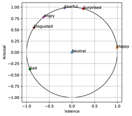
Emotion representation: We represented emotion labels as points in the 2D valence-arousal space (VA, Russell 1980). Particularly, we used a manually annotated part of the large-scale AffectNet database (Mollahosseini et al., 2017). For all samples of a particular emotion in the AffectNet data, we computed the centroid (data mean) of the valence and arousal values. The resulting -normalized 2D vectors constituted our emotion representation as depicted in Fig. 3. The normalization is akin to assuming that the modeled emotions are of the same intensity. In our experiments, the emotion ‘neutral’ was represented by the origin. Such an emotion embedding allowed us to take into account prior knowledge about the angular proximity of emotions in the VA space, while keeping the representation simple and interpretable for post-hoc manipulations.
Kernel design: We took the kernels , to be Gaussian on the landmark representation space and the emotion representation space, with respective bandwidth and . was assumed to be unless specified otherwise.
4.2 Quantitative Performance Assessment
In this section we provide a quantitative assessment of the proposed vITL approach.
Performance measures: We applied two metrics to quantify the performance of the compared systems, namely the test mean squared error (MSE) and emotion classification accuracy. The classification accuracy can be thought of as an indirect evaluation. To compute this measure, for each dataset we trained a ResNet-18 classifier to recognize emotions from ground-truth landmark edge maps (as depicted in Fig. 2). The trained network was then used to compute classification accuracy over the predictions at test time. To rigorously evaluate outputs for each split of the data, we used a classifier trained on RaFD to evaluate KDEF predictions and vice-versa; this also allowed us to make the problem more challenging. The ResNet-18 network was appropriately modified to take grayscale images as input. During training, we used random horizontal flipping and cropping between 90-100% of the original image size to augment the data. All the images were finally resized to and fed to the network. The network was trained from scratch using the stochastic gradient descent optimizer with learning rate and momentum set to and , respectively. The training was carried out for epochs with a batch size of .
We report the mean and standard deviation of the aforementioned metrics over ten 90%-10% train-test splits of the data. The test set for each split is constructed by removing of the identities from the data. For each split, the best and values were determined by -fold and -fold cross-validation on KDEF and RaFD, respectively.
Baseline: We used the popular StarGAN (Choi et al., 2018) system as our baseline. Other GAN-based studies use additional information and are not directly comparable to our setting. For fair comparison, the generator and discriminator were modified to be fully-connected networks that take vectorized landmarks as input. In particular, was an encoder-decoder architecture where the target emotion, represented as a 2D emotion encoding as for our case, was appended at the bottleneck layer. It contained approximately one million parameters, which was chosen to be comparable with the number of coefficients in vITL ( for KDEF). ReLU activation function was used in all layers except before bottleneck in and before penultimate layers of both and . We used their default parameter values in the code.333The code is available at https://github.com/yunjey/stargan. Experiments over each split of KDEF and RaFD were run for 50K and 25K iterations, respectively.
MSE results: The test MSE for the compared systems is summarized in Table 1. As the table shows, the vITL technique outperforms StarGAN on both datasets. One can observe low reconstruction cost for vITL in both the single and the joint emotional input case. Interestingly, a performance gain is obtained with vITL joint on the RaFD data in MSE sense. We hypothesize that this is due to the joint model benefiting from input landmarks for other emotions in the small data regime (only samples per emotion for RaFD). Despite our best efforts, we found it quite difficult to train StarGAN reliably and the diversity of its outputs was low.
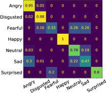
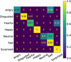
Classification results: The emotion classification accuracies are available in Table 2. The classification results clearly demonstrate the improved performance and the higher quality of the generated emotion of vITL over StarGAN; the latter also produces predictions with visible face distortions as it is illustrated in Section 4.4. To provide further insight into the classification performance we also show the confusion matrices for the joint vITL model on a particular split of KDEF and RaFD datasets in Fig. 4. For both the datasets, the classes ‘happy’ and ‘surprised’ are easiest to detect. Some confusions arise between the classes ‘neutral’ vs ‘sad’ and ‘fearful’ vs ‘surprised’. Such mistakes are expected when only using landmark locations for recognizing emotions.
| Methods | KDEF frontal | RaFD frontal |
|---|---|---|
| vITL: neutral | ||
| vITL: fearful | ||
| vITL: angry | ||
| vITL: disgusted | ||
| vITL: happy | ||
| vITL: sad | ||
| vITL: surprised | ||
| vITL: Joint | ||
| StarGAN |
| Methods | KDEF frontal | RaFD frontal |
|---|---|---|
| vITL: neutral | ||
| vITL: fearful | ||
| vITL: angry | ||
| vITL: disgusted | ||
| vITL: happy | ||
| vITL: sad | ||
| vITL: surprised | ||
| vITL: Joint | ||
| StarGAN |
4.3 Analysis of Additional Properties of vITL
This section is dedicated to the effect of the choice of (in kernel ) and to the robustness of vITL w.r.t. partial observation.
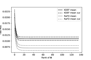
Influence of in the matrix-valued kernel : Here, we illustrate the effect of matrix (see (5)) on the vITL estimator and show that a good choice of can lead to lower dimensional models, while preserving the quality of the prediction. The choice of is built on the knowledge that the empirical covariance matrices of the output training data contains structural information that can be exploited with vRKHS (Kadri et al., 2013). In order to investigate this possibility, we performed the singular value decomposition of which gives the eigenvectors collected in matrix . For a fixed rank , define , set and train a vITL system with the resulting . While in this case is no more invertible, each coefficient from Lemma 3.1 belongs to the -dimensional subspace of generated by the eigenvectors associated to the largest eigenvalues of . This makes a reparameterization possible and leads to a decrease in the size of the model, going from parameters to . We report in Fig. 5 the resulting test MSE performance (mean standard deviation) obtained from different splits, and empirically observe that suffices to preserve the optimal performances of the model.
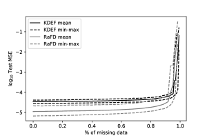
Learning under a partial observation regime: To assess the robustness of vITL w.r.t. missing data, we considered a random mask ; a sample was used for learning only when . Thus, the percentage of missing data was . The experiment was repeated for splits of the dataset, and on each split we averaged the results using different random masks . The resulting test MSE of the predictor as a function of is summarized in Fig. 6. As it can be seen, the vITL approach is quite stable in the presence of missing data on both datasets.
4.4 Qualitative Analysis
In this section we show example outputs produced by vITL in the context of discrete and continuous emotion generation. While the former is the classical task of synthesis given input landmarks and target emotion label, the latter serves to demonstrate a key benefit of our approach, which is the ability to synthesize meaningful outputs while continuously traversing the emotion embedding space.
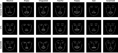
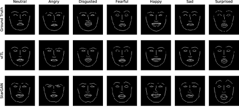
Discrete emotion generation: In Fig. 7 and 8 we show qualitative results for generating landmarks using discrete emotion labels present in the datasets. For vITL, not only are the emotions recognizable, but landmarks on the face boundary are reasonably well synthesized and other parts of the face visibly less distorted when compared to StarGAN. The identity in terms of the face shape is also better preserved.
Continuous emotion generation: Starting from neutral emotion, continuous generation in the radial direction is illustrated in Fig. 9. The landmarks vary smoothly and conform to the expected intensity variation in each emotion on increasing the radius of the vector in VA space. We also show in Fig. 10 the capability to generate intermediate emotions by changing the angular position, in this case from ‘happy’ to ‘surprised’. For a more fine-grained video illustration traversing from ‘happy’ to ‘sad’ along the circle, see the GitHub repository.
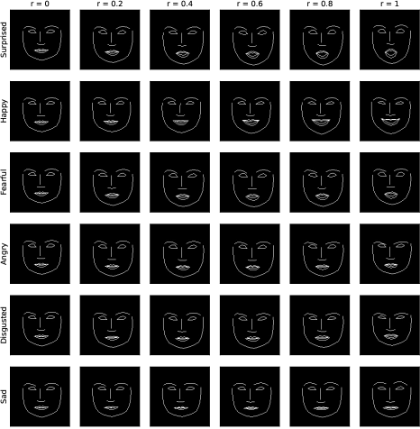

These experiments and qualitative results demonstrate the efficiency of the vITL approach in emotion transfer.
5 Conclusion
In this paper we introduced a novel approach to style transfer based on function-valued regression, and exemplified it on the problem of emotion transfer. The proposed vector-valued infinite task learning (vITL) framework relies on operator-valued kernels. vITL (i) is capable of encoding and controlling continuous style spaces, (ii) benefit from a representer theorem for efficient computation, and (iii) facilitates regularity control via the choice of the underlying kernels. The framework can be extended in several directions. Other losses (Sangnier et al., 2016; Laforgue et al., 2020) can be leveraged to produce outlier-robust or sparse models. Instead of being chosen prior to learning, the input kernel could be learned using deep architectures (Mehrkanoon and Suykens, 2018; Liu et al., 2020) opening the door to a wide range of applications.
6 Proofs
This section contains the proofs of our auxiliary lemmas.
Proof 6.1
(Lemma 3.1) For all , let denote the function defined by . Similarly, for all , stands for the function where . Let us take the finite-dimensional subspace
The space can be decomposed as and its orthogonal complement: . The existence of follows from the coercivity of (i.e. as ) which is the consequence of the quadratic regularizer and the lower boundedness of . Uniqueness comes from the strong convexity of the objective. Let us decompose , and take any . Then ,
(a) follows from the reproducing property in , (b) is a consequence of the reproducing property in , and (c) comes from the decomposition . This means that , and hence . Since we conclude that and get that there exist coefficients such that . This evaluates for all to
as claimed in (7).
Proof 6.2
Acknowledgements
A.L. and S.P. were funded by the research chair Data Science & Artificial Intelligence for Digitalized Industry and Services at Télécom Paris. ZSz benefited from the support of the Europlace Institute of Finance and that of the Chair Stress Test, RISK Management and Financial Steering, led by the French École Polytechnique and its Foundation and sponsored by BNP Paribas.
References
- Álvarez et al. (2012) M. A. Álvarez, L. Rosasco, and N. D. Lawrence. Kernels for vector-valued functions: a review. Foundations and Trends in Machine Learning, 4(3):195–266, 2012.
- Barricelli et al. (2019) Barbara Rita Barricelli, Elena Casiraghi, and Daniela Fogli. A survey on digital twin: Definitions, characteristics, applications, and design implications. IEEE Access, 7:167653–167671, 2019.
- Blanz and Vetter (1999) Volker Blanz and Thomas Vetter. A morphable model for the synthesis of 3D faces. In Conference on Computer Graphics and Interactive Techniques (SIGGRAPH), pages 187–194, 1999.
- Brault et al. (2019) Romain Brault, Alex Lambert, Zoltán Szabó, Maxime Sangnier, and Florence d’Alché-Buc. Infinite task learning in RKHSs. In International Conference on Artificial Intelligence and Statistics (AISTATS), pages 1294–1302, 2019.
- Carmeli et al. (2006) Claudio Carmeli, Ernesto De Vito, and Alessandro Toigo. Vector valued reproducing kernel Hilbert spaces of integrable functions and Mercer theorem. Analysis and Applications, 4:377–408, 2006.
- Carmeli et al. (2010) Claudio Carmeli, Ernesto De Vito, Alessandro Toigo, and Veronica Umanitá. Vector valued reproducing kernel Hilbert spaces and universality. Analysis and Applications, 8(1):19–61, 2010.
- Choi et al. (2018) Yunjey Choi, Minje Choi, Munyoung Kim, Jung-Woo Ha, Sunghun Kim, and Jaegul Choo. StarGAN: Unified generative adversarial networks for multi-domain image-to-image translation. In Conference on Computer Vision and Pattern Recognition (CVPR), pages 8789–8797, 2018.
- Ding et al. (2018) Hui Ding, Kumar Sricharan, and Rama Chellappa. ExprGAN: Facial expression editing with controllable expression intensity. In Conference on Artificial Intelligence (AAAI), pages 6781–6788, 2018.
- Ekman et al. (2002) Paul Ekman, Wallace Friesen, and Joseph Hager. Facial action coding system: The manual. Salt LakeCity, UT: Research Nexus., 2002.
- El Guennouni et al. (2002) A El Guennouni, Khalide Jbilou, and AJ Riquet. Block Krylov subspace methods for solving large Sylvester equations. Numerical Algorithms, 29(1):75–96, 2002.
- Evgeniou and Pontil (2004) Theodoros Evgeniou and Massimiliano Pontil. Regularized multi–task learning. In ACM SIGKDD International Conference on Knowledge Discovery and Data Mining (KDD), pages 109–117, 2004.
- Evgeniou et al. (2005) Theodoros Evgeniou, Charles Micchelli, and Massimiliano Pontil. Learning multiple tasks with kernel methods. Journal of Machine Learning Research, 6:615–637, 2005.
- Fu et al. (2018) Zhenxin Fu, Xiaoye Tan, Nanyun Peng, Dongyan Zhao, and Rui Yan. Style transfer in text: Exploration and evaluation. In Conference on Artificial Intelligence (AAAI), pages 663–670, 2018.
- Gatys et al. (2016) Justin J. Gatys, Alexandre A., and F.-F Li. Perceptual losses for real-time style transfer and super-resolution. In European Conference on Computer Vision (ECCV), pages 694–711, 2016.
- Geirhos et al. (2019) Robert Geirhos, Patricia Rubisch, Claudio Michaelis, Matthias Bethge, Felix A. Wichmann, and Wieland Brendel. ImageNet-trained CNNs are biased towards texture; increasing shape bias improves accuracy and robustness. In International Conference on Learning Representations (ICLR), 2019.
- Geng et al. (2018) Jiahao Geng, Tianjia Shao, Youyi Zheng, Yanlin Weng, and Kun Zhou. Warp-guided GANs for single-photo facial animation. ACM Transactions on Graphics, 37(6):1–12, 2018.
- Goodfellow et al. (2014) Ian J. Goodfellow, Jean Pouget-Abadie, Mehdi Mirza, Bing Xu, David Warde-Farley, Sherjil Ozair, Aaron Courville, and Yoshua Bengio. Generative adversarial nets. In Advances in Neural Information Processing Systems (NIPS), pages 2672–2680, 2014.
- Grinstein et al. (2018) Eric Grinstein, Ngoc QK Duong, Alexey Ozerov, and Patrick Pérez. Audio style transfer. In International Conference on Acoustics, Speech and Signal Processing (ICASSP), pages 586–590, 2018.
- Jing et al. (2020) Yongcheng Jing, Yezhou Yang, Zunlei Feng, Jingwen Ye, Yizhou Yu, and Mingli Song. Neural style transfer: A review. IEEE Transactions on Visualization and Computer Graphics, 26(11):3365–3385, 2020.
- Kadri et al. (2010) Hachem Kadri, Emmanuel Duflos, Philippe Preux, Stéphane Canu, and Manuel Davy. Nonlinear functional regression: a functional RKHS approach. In International Conference on Artificial Intelligence and Statistics (AISTATS), pages 374–380, 2010.
- Kadri et al. (2013) Hachem Kadri, Mohammad Ghavamzadeh, and Philippe Preux. A generalized kernel approach to structured output learning. In International Conference on Machine Learning (ICML), pages 471–479, 2013.
- Kadri et al. (2016) Hachem Kadri, Emmanuel Duflos, Philippe Preux, Stéphane Canu, Alain Rakotomamonjy, and Julien Audiffren. Operator-valued kernels for learning from functional response data. Journal of Machine Learning Research, 17(20):1–54, 2016.
- Kazemi and Sullivan (2014) Vahid Kazemi and Josephine Sullivan. One millisecond face alignment with an ensemble of regression trees. In Conference on Computer Vision and Pattern Recognition (CVPR), pages 1867–1874, 2014.
- Laforgue et al. (2020) Pierre Laforgue, Alex Lambert, Luc Brogat-Motte, and Florence d’Alché Buc. Duality in RKHSs with infinite dimensional outputs: Application to robust losses. In International Conference on Machine Learning (ICML), pages 5598–5607, 2020.
- Langner et al. (2010) Oliver Langner, Ron Dotsch, Gijsbert Bijlstra, Daniel HJ Wigboldus, Skyler T Hawk, and AD Van Knippenberg. Presentation and validation of the Radboud faces database. Cognition and emotion, 24(8):1377–1388, 2010.
- Lim et al. (2020) Kendrik Yan Hong Lim, Pai Zheng, and Chun-Hsien Che. A state-of-the-art survey of digital twin: techniques, engineering product lifecycle management and business innovation perspectives. Journal of Intelligent Manufacturing, 31:1313–1337, 2020.
- Liu et al. (2020) Feng Liu, Wenkai Xu, Jie Lu, Guangquan Zhang, Arthur Gretton, and Danica J. Sutherland. Learning deep kernels for non-parametric two-sample tests. In International Conference on Machine Learning (ICML), pages 6316–6326, 2020.
- Lundqvist et al. (1998) Daniel Lundqvist, Anders Flykt, and Arne Öhman. The Karolinska directed emotional faces (KDEF). CD ROM from Department of Clinical Neuroscience, Psychology section, Karolinska Institutet, 91(630):2–2, 1998.
- Meanti et al. (2020) Giacomo Meanti, Luigi Carratino, Lorenzo Rosasco, and Alessandro Rudi. Kernel methods through the roof: handling billions of points efficiently. In Advances in Neural Information Processing Systems (NeurIPS), 2020.
- Mehrkanoon and Suykens (2018) Siamak Mehrkanoon and Johan A. K. Suykens. Deep hybrid neural-kernel networks using random Fourier features. Neurocomputing, 298:46–54, 2018.
- Micchelli and Pontil (2005) Charles Micchelli and Massimiliano Pontil. On learning vector-valued functions. Neural Computation, 17:177–204, 2005.
- Mikołajczyk and Grochowski (2018) Agnieszka Mikołajczyk and Michał Grochowski. Data augmentation for improving deep learning in image classification problem. In International Interdisciplinary PhD Workshop (IIPhDW), pages 117–122, 2018.
- Mollahosseini et al. (2017) Ali Mollahosseini, Behzad Hasani, and Mohammad H Mahoor. AffectNet: A database for facial expression, valence, and arousal computing in the wild. IEEE Transactions on Affective Computing, 10(1):18–31, 2017.
- Pedrick (1957) George Pedrick. Theory of reproducing kernels for Hilbert spaces of vector valued functions. PhD thesis, 1957.
- Pumarola et al. (2018) Albert Pumarola, Antonio Agudo, Aleix M Martinez, Alberto Sanfeliu, and Francesc Moreno-Noguer. GANimation: Anatomically-aware facial animation from a single image. In European Conference on Computer Vision (ECCV), pages 818–833, 2018.
- Puy and Pérez (2019) Gilles Puy and Patrick Pérez. A flexible convolutional solver for fast style transfers. In Conference on Computer Vision and Pattern Recognition (CVPR), pages 8963–8972, 2019.
- Qiao et al. (2018) Fengchun Qiao, Naiming Yao, Zirui Jiao, Zhihao Li, Hui Chen, and Hongan Wang. Geometry-contrastive GAN for facial expression transfer. Technical report, 2018. (https://arxiv.org/abs/1802.01822).
- Rudi et al. (2017) Alessandro Rudi, Luigi Carratino, and Lorenzo Rosasco. FALKON: An optimal large scale kernel method. In Advances in Neural Information Processing Systems (NIPS), pages 3891–3901, 2017.
- Russell (1980) James A Russell. A circumplex model of affect. Journal of Personality and Social Psychology, 39(6):1161–1178, 1980.
- Sangnier et al. (2016) Maxime Sangnier, Olivier Fercoq, and Florence d’Alché Buc. Joint quantile regression in vector-valued RKHSs. Advances in Neural Information Processing Systems (NIPS), pages 3693–3701, 2016.
- Saragih et al. (2009) Jason M. Saragih, Simon Lucey, and Jeffrey F. Cohn. Face alignment through subspace constrained mean-shifts. In International Conference on Computer Vision (ICCV), pages 1034–1041, 2009.
- Scherhag et al. (2018) Ulrich Scherhag, Dhanesh Budhrani, Marta Gomez-Barrero, and Christoph Busch. Detecting morphed face images using facial landmarks. In International Conference on Image and Signal Processing (ICISP), pages 444–452, 2018.
- Schölkopf et al. (2001) Bernhard Schölkopf, John C Platt, John Shawe-Taylor, Alex J. Smola, and Robert C Williamson. Estimating the support of a high-dimensional distribution. Neural computation, 13(7):1443–1471, 2001.
- Song et al. (2018) Lingxiao Song, Zhihe Lu, Ran He, Zhenan Sun, and Tieniu Tan. Geometry guided adversarial facial expression synthesis. In International Conference on Multimedia (MM), pages 627–635, 2018.
- Susskind et al. (2008) Joshua M Susskind, Geoffrey E Hinton, Javier R Movellan, and Adam K Anderson. Generating facial expressions with deep belief nets. In Affective Computing, chapter 23. IntechOpen, 2008.
- Takeuchi et al. (2006) Ichiro Takeuchi, Quoc Le, Timothy Sears, and Alexander Smola. Nonparametric quantile estimation. Journal of Machine Learning Research, 7:1231–1264, 2006.
- Tao et al. (2019) Fei Tao, He Zhang, Ang Liu, and A. Y. C. Nee. Digital twin in industry: State-of-the-art. IEEE Transactions on Industrial Informatics, 15(4):2405 – 2415, 2019.
- Tautkute et al. (2018) Ivona Tautkute, T. Trzciński, and Adam Bielski. I know how you feel: Emotion recognition with facial landmarks. Conference on Computer Vision and Pattern Recognition Workshops (CVPRW), pages 1959–19592, 2018.
- Ulyanov et al. (2016) Dmitry Ulyanov, Vadim Lebedev, Andrea Vedaldi, and Victor Lempitsky. Texture networks: Feed-forward synthesis of textures and stylized images. In International Conference on Machine Learning (ICML), pages 1349–1357, 2016.
- Vemulapalli and Agarwala (2019) Raviteja Vemulapalli and Aseem Agarwala. A compact embedding for facial expression similarity. In Conference on Computer Vision and Pattern Recognition (CVPR), pages 5683–5692, 2019.
- Wynen et al. (2018) Daan Wynen, Cordelia Schmid, and Julien Mairal. Unsupervised learning of artistic styles with archetypal style analysis. In Advances in Neural Information Processing Systems (NeurIPS), pages 6584–6593, 2018.
- Yao et al. (2020) Xu Yao, Gilles Puy, Alasdair Newson, Yann Gousseau, and Pierre Hellier. High resolution face age editing. In International Conference on Pattern Recognition (ICPR), 2020.
- Zhang et al. (2015) Zheng Zhang, Long Wang, Qi Zhu, Shu-Kai Chen, and Yan Chen. Pose-invariant face recognition using facial landmarks and Weber local descriptor. Knowledge-Based Systems, 84:78–88, 2015.
- Zhu et al. (2017) Jun-Yan Zhu, Taesung Park, Phillip Isola, and Alexei A Efros. Unpaired image-to-image translation using cycle-consistent adversarial networks. In International Conference on Computer Vision (ICCV), pages 2223–2232, 2017.