Training Federated GANs with Theoretical Guarantees: A Universal Aggregation Approach
Abstract
Recently, Generative Adversarial Networks (GANs) have demonstrated their potential in federated learning, i.e., learning a centralized model from data privately hosted by multiple sites. A federated GAN jointly trains a centralized generator and multiple private discriminators hosted at different sites. A major theoretical challenge for the federated GAN is the heterogeneity of the local data distributions. Traditional approaches cannot guarantee to learn the target distribution, which is a mixture of the highly different local distributions. This paper tackles this theoretical challenge, and for the first time, provides a provably correct framework for federated GAN. We propose a new approach called Universal Aggregation, which simulates a centralized discriminator via carefully aggregating the mixture of all private discriminators. We prove that a generator trained with this simulated centralized discriminator can learn the desired target distribution. Through synthetic and real datasets, we show that our method can learn the mixture of largely different distributions where existing federated GAN methods fail. 111code available at: https://github.com/yz422/UAGAN
1 Introduction
Generative Adversarial Networks (GANs) have attracted much attention due to their ability to generate realistic-looking synthetic data [7, 50, 27, 41, 6, 18]. In order to obtain a powerful GAN model, one needs to use data with a wide range of characteristics [36]. However, these diverse data are often owned by different sources, and to acquire their data is often infeasible. For instance, most hospitals and research institutions are unable to share data with the research community, due to privacy concerns [2, 30, 20, 8] and government regulations [16, 40].
To circumvent the barrier of data sharing for GAN training, one may resort to Federated Learning (FL), a promising new decentralized learning paradigm [28]. In FL, one trains a centralized model but only exchanges model information with different data sources. Since the central model has no direct access to data at each source, privacy concerns are alleviated [48, 15]. This opens the opportunity for a federated GAN, i.e., a centralized generator with multiple local and privately hosted discriminators [11]. Each local discriminator is only trained on its local data and provides feedback to the generator w.r.t. synthesized data (e.g., gradient). A federated GAN empowers GAN with much more diversified data without violating privacy constraints.
Despite the promises, a convincing approach for training a federated GAN remains unknown. The major challenge comes from the non-identical local distributions from multiple data sources/entities. The centralized generator is supposed to learn a mixture of these local distributions from different entities, whereas each discriminator is only trained on local data and learns one of the local distributions. The algorithm and theoretical guarantee of traditional single-discriminator GAN [7] do not easily generalize to this federated setting. A federated GAN should integrate feedback from local discriminators in an intelligent way, so that the generator can ‘correctly’ learn the mixture distribution. Directly averaging feedbacks from local discriminators [11] results in a strong bias toward common patternsowever, such non-identical distribution setting is classical in federated learning [51, 43, 37] and characteristic of local data improves the diversity of data.
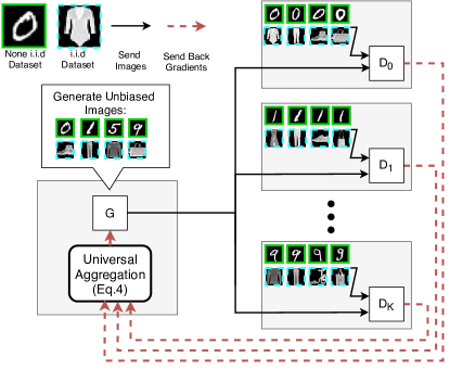
In this paper, we propose the first theoretically guaranteed federated GAN, that can correctly learn the mixture of local distributions. Our method, called Universal Aggregation GAN (UA-GAN), focuses on the odds value rather than the predictions of local discriminators. We simulate an unbiased centralized discriminator whose odds value approximates that of the mixture of local discriminators. We prove that by aggregating gradients from local discriminators based on the odds value of the central discriminator, we are guaranteed to learn the desired mixture of local distributions.
A second theoretical contribution of this paper is an analysis of the quality of the federated GAN when the local discriminators cannot perfectly learn with local datasets. This is a real concern in a federated learning setting; the quantity and quality of local data can be highly variant considering the limitation of real-world institutions/sites. Classical theoretical analysis of GAN [7] assumes an optimal discriminator. To understand the consequence of suboptimal discriminators, we develop a novel analysis framework of the Jensen-Shannon Divergence loss [7, 24] through the odds value of the local discriminators. We show that when the local discriminators behave suboptimally, the approximation error of the learned generator deteriorates linearly to the error.
It is worth noting that our theoretical result on suboptimality also applies to the classical GAN. To the best of our knowledge, this is the first suboptimality bound on the federated or classical GAN.
In summary, the contributions are threefold.
-
•
We propose UA-GAN, a novel federated GAN approach that aggregates feedback from local discriminators through their odds value rather than posterior probability.
-
•
We prove that UA-GAN correctly learns the mixture of local distributions when they are perfectly modeled by local discriminators.
-
•
We prove when the discriminators are suboptimal in modeling their local distributions, the generator’s approximation error is also linear. We also show that our bound is tight.
We show with various experiments that our method (UA-GAN) outperforms the state-of-the-art federated GAN approaches both qualitatively and quantitatively.
Training on large scale heterogeneous datasets makes it possible to unleash the power of GANs. Federated GANs show their promise in utilizing unlimited amount of sensitive data without privacy and regulatory concerns. Our method, as the first theoretically guaranteed GAN, will be one step further in building such a foundation. Fig. 1 shows the workflow of UA-GAN.
2 Related Work
The Generative Adversarial Networks (GANs) have enjoyed much success in various machine learning and computer vision tasks [50, 27, 41, 6, 18]. Numerous methods are proposed for GAN training, such as Spectral Normalization (SN) [33], zero-centered gradient penalty [31, 44], WGAN [3] , WGAN-GP [10], WGAN-TS [25], WGAN-QC [26] etc. A common approach in practice is the conditional GAN (cGAN) [32], which uses supervision from data (e.g., class labels) to improve GAN’s performance.
Multi-discriminator/-generator GANs have been proposed for various learning tasks. To train these GANs, one common strategy is to directly exchange generator/discriminator model parameters during training [47, 11]. This is very expensive in communication; a simple ResNet18 [12] has 11 million parameters (40MB). Closest to us is MD-GAN [11], which aggregates feedbacks (gradients) from local discriminators through averaging. It also swaps parameters between discriminators. None of these methods provide theoretical guarantee as ours. Meanwhile, our method is the only one without model swapping, and thus is much more efficient in bandwidth consumption.
Federated Learning (FL) [15, 29] offers the opportunity to integrate sensitive datasets from multiple sources through distributed training. Many works have been done tackling practical concerns in FL, such as convergence under Non-IID data assumption [49, 23, 21], decentralized SGD without freezing parameters [38, 35], communication efficiency [17, 22], provable privacy guarantees [1, 45]. Federated GAN is also of great interest from a federated learning perspective. A successful federated GAN makes it possible to train a centralized model (e.g., a classifier) using data synthesized by the centralized generator. This becomes a solution when existing trained FL model needs to be replaced and updated by advanced machine learning approaches , as one can retrain the model at any time using the generator. It also alleviates some privacy concerns of FL, e.g., the gradient leakage problem [52].
3 Method
To introduce our algorithm, we first introduce notations and formalize the mixture distribution learning problem. Next, we present our Universal Aggregation approach and prove that it is guaranteed to learn the target mixture distribution. We also analyze the suboptimality of the model when local discriminators are suboptimal. For ease of exposition, we mostly use ordinary GAN to illustrate the algorithm and prove its theoretical properties. At the end of this section, we extend the algorithm, as well as its theoretical guarantees, to conditional GAN (cGAN) [32]. The empirical results in this work are established on the cGAN since its training is much more controllable, thanks to the additional supervision by the auxiliary variable (e.g., classes of images).
Notations and problem formulation. We assume a cross-silo FL setting [15], i.e., entities hosting private datasets , with size . The total data size . The overall goal is to learn a target mixture distribution
| (1) |
in which a component distributions is approximated by the empirical distribution from the -th local dataset . The mixing weight is computed using the fraction of dataset : . In general, different mixture components and may (but not necessarily) be non-identical, namely, , such that .
Universal Aggregation GAN: Now we are ready to introduce our multi-discriminator aggregation framework. A pseudo-code of UA framework can be found in Algorithm 1. We have a centralized (conditional) generator seeking to learn the global distribution . In each local site, a discriminator has access to local dataset . Note data in are only sampled from . During training, the generator generates a batch of synthetic data to all sites. The -th discriminator seeks to minimize the cross entropy loss of GAN from a local perspective [7]:
| (2) |
To formalize the generator training, we first introduce odds value. It is an essential quantity for our algorithm and its analysis.
Definition 1 (odds value).
Given a probability , its odds value is . Note the definition requires .
Also it is straightforward to see .
The central idea of UA Framework is to simulate a centralized discriminator which behaves like the mixture of all local discriminators (in terms of odds value). A well behaved can then train the centralized generator using its gradient, just like in a classical GAN.
We design so that its odds value is identical to the mixture of the odds values of local discriminators:
| (3) |
Given , we can compute as
| (4) |
Once the central discriminator is simulated, the generator can be computed by minimizing the generator loss :
| (5) |
Note that mathematically, Eq. (5) can be directly written in terms of local discriminators ’s (by substituting in Eqs (3) and (4)). In implementation, the simulated central discriminator can be written as a pytorch or tensorflow layer.
Intuition. The reason we define ’s behavior using a mixture of odds values instead of a mixture of the predictions is mathematical. It has been shown in [7] that a perfect discriminator learning a data distribution and a fixed generator distribution satisfies . It can be shown that only with the odds value equivalency, this optimal solution of the central discriminator can be recovered if each individual discriminator is optimal, i.e., . This is not true if we define the central discriminator behavior using the average prediction, i.e., . More details can be found in Theorem (1) and its proof.
Remark 1 (Privacy Safety).
For federated learning, it is essential to ensure information of real data are not leaked outside the local site. This privacy safety is guaranteed in our method. To optimize w.r.t. Eq. (5), we only need to optimize the second term and use gradient on synthetic images from local discriminators.
One important concern is about the optimal discriminator condition. is designed to be optimal only when ’s are optimal. We need to investigate the consequence if the local discriminators ’s are suboptimal. We will provide an error bound of the learned distribution w.r.t., the suboptimality of ’s in Corollary (1).
3.1 Theoretical Analysis of UA-GAN
In this section, we prove the theoretical guarantees of UA-GAN. First, we prove the correctness of the algorithm. We show that if all local discriminators can perfectly learn from their local data, the algorithm is guaranteed to recover the target distribution (Eq. (1)). Second, we discuss the quality of the learned generator distribution when the local discriminators are suboptimal, due to real-world constraints, e.g., insufficient local data. We show that the error of the learned distribution is linear to the suboptimality of the local discriminators. All results in this section are for original (unconditional) GANs. But they can be extended to conditional GANs (see Sec. (3.2)). Due to space constraints, we only state the major theorems and leave their proofs to the supplemental material.
Correctness of UA-GAN
The correctness theorem assumes all local discriminators behave optimally.
Assumption 1 (Optimal Local Discriminator).
Assume all local discriminators are optimal, i.e., they learn to predict whether a data is true/fake perfectly. Let be the probability of the current generator . A local discriminator is optimal iff .
Theorem (1) states the unbiasedness of UA-GAN: with optimal local discriminators, the generator learns the target distribution.
Theorem 1 (Correctness).
Suppose all discriminators ’s are optimal. is computed via Eq. (3). Denote by the density function of data generated by . Let be the optimal distribution w.r.t. the Jenson Shannon divergence loss :
| (6) |
We have equals to the true distribution, formally, .
The proof mainly establishes that when ’s are optimal, is also optimal. With the optimality of proved, the rest follows the correctness proof of the classic GAN (Theorem 1 in [7]). More details are in the supplemental material.
Analysis of the Suboptimal Setting
In centralized learning setting, an optimal discriminator is a reasonable assumption since the model has access to all (hopefully sufficient) data. However, in federated GAN setting, available data in some site may be limited. One natural question in this limited data scenario is: how would the generator behave if some local discriminators are suboptimal? We address this theoretical question.
We first focus on a single discriminator case. We show the behavior of a perturbed version of Jensen-Shannon divergence loss [9, 24, 5]. The suboptimality of a central discriminator is measured by the deviation in terms of the odds value. Denote by the generator distribution of the current . Ideally, the odds value of an optimal discriminator should be . We show that a suboptimal with deviation from the ideal odds value will result in suboptimality in the target distribution.
Theorem 2 (Suboptimality Bound for a Single Discriminator).
Suppose a discriminator is a perturbed version of the optimal discriminator , s.t. with and . Let be the optimal distribution of the Jensen-Shannon divergence loss based on the perturbed discriminator
| (7) |
Then satisfies .
This theorem shows that the ratio of the learned distribution is close to the target true distribution when the suboptimality of is small. To the best of our knowledge, this is the first bound on the consistency of Jensen-Shannon divergence with suboptimal discriminator, even for a classical GAN.
Next, we show that the bound is also tight.
Theorem 3 (Tightness of the Bound in Theorem (2)).
Given a perturbed discriminator of the optimal one , s.t. with and . The optimal distribution as in Eq. (7) satisfies , .
Next we extend these bounds for a single discriminator to our multi-discriminator setting. This is based on Theorem (2) and the linear relationship between the local discriminators and the central discriminator.
Corollary 1 (Suboptimality Bound for UA-GAN).
Assume suboptimal local discriminators are the perturbed versions of the optimal ones . And the suboptimality is bounded as: with , . The centralized discriminator is computed using these perturbed local discriminators such that . Let be the optimal distribution of the Jensen-Shannon divergence loss based on the perturbed UA discriminator
| (8) |
Then satisfies . In particular, the optimal distribution has total variation distance to the target distribution .
Note that the lowerbound of the suboptimality for single discriminator (Theorem (3)) can also be extended to UA-GAN similarly.
Remark 2.
The consistency gap in Corollary (1) assumes a uniform suboptimality bounded for all local discriminators. In practice, such assumption may not be informative if the sizes of ’s data are highly imbalanced. It would be interesting to relax such assumption and investigate the guarantees of UA-GAN w.r.t. the expected suboptimality of ’s.
3.2 Universal Aggregation Framework for Conditional GAN
Our algorithm and analysis on unconditional GANs can be generalized to the more practical Conditional GAN [32]. A conditional GAN learns the joint distribution of . Here represents an image or a vectorized data, and is an auxiliary variable to control the mode of generated data (e.g., the class label of an image/data). Conditional GAN is much better to train in practice and is the common choice in most existing works. This is indeed the setting we use in our experiments.
The target distribution of the learning problem becomes a joint mixture distribution:
in which and is the proportion of class data within the -th local dataset . We assume , and the dictionary of and its fractions in each , are known to the public. In practice, such knowledge will be used for generating . Formally, .
To design the UA-GAN for the conditional GAN, the odds value aggregation in formula Eq. (3) needs to be adapted to:
The computation of and the update of and ’s need to be adjusted accordingly. The theoretical guarantees for unconditional GANs can also be established for a conditional GAN. Due to space limitation, we leave details to the supplemental material.
4 Experiments
On synthetic and real-world datasets, we verify that UA-GAN can learn the target distribution from both i.i.d and non-identical local datasets. We focus on conditional GAN [32] setting as it is the common choice in practice.
| UA-GAN |  |
| Avg-GAN |  |
| MD-GAN |  |
4.1 Synthetic Experiment
We evaluate UA-GAN on a toy dataset. See Fig. 2 first row. The toy dataset has 4 datasets, generated by 4 Gaussians centered at (10, 10), (10,-10), (-10,10), (-10,-10) with variance 0.5. Data samples are shown as blue points. The central generator takes Gaussian noise centered at with variance of 0.5 (green points) and learns to transform them into points matching the mixture distribution (orange points). The first figure shows the generator successfully recovers the Gaussian mixture. The contours show the central discriminator calculated according to Eq. 3. The generated points (orange) are evenly distributed near the 4 local Gaussians’ centers. The 2nd to 5th figures show the prediction of the local discriminators (’s), overlaid with their respective samples in blue.
Meanwhile, we show in the second row the results of the average scheme, called Avg-GAN, which averages local discriminators’ outputs to train the generator. The first figure shows that the learned distribution is almost flat. The generated samples (orange) collapse near the origin. Although each individual discriminator can provide valid gradient information (see 2nd to 5th figures for ’s), naively averaging their outputs cannot achieve the target distribution, when the distributions are symmetric. We show the results of the MD-GAN by [11] in the third row. MD-GAN also adopts the average scheme, but randomly shuffle discriminators parameters during training. Similar to Avg-GAN, MD-GAN cannot learn the four Gaussians.
| Dataset | non-identical Mnist + Fashion | non-identical Mnist + Font | ||||
| Accuracy | IS | FID | Accuracy | IS | FID | |
| Real | 0.943 | 3.620 0.021 | 0 | 0.994 | 2.323 0.011 | 0 |
| Centralized GAN | 0.904 | 3.437 0.021 | 8.35 | 0.979 | 1.978 0.009 | 17.62 |
| Avg GAN | 0.421 | 4.237 0.023 | 72.80 | 0.822 | 1.517 0.004 | 85.81 |
| MD-GAN | 0.349 | 2.883 0.020 | 102.00 | 0.480 | 2.090 0.007 | 69.63 |
| UA-GAN | 0.883 | 3.606 0.020 | 24.60 | 0.963 | 1.839 0.006 | 24.73 |
4.2 Real-World Mixture Datasets
We evaluate our method on several mixture datasets, both i.i.d and non-identical.
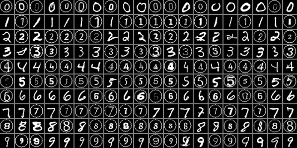
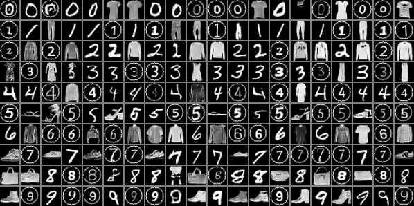
Datasets. Three real-world datasets are utilized to construct the mixture datasets: MNIST [19], Fashion-MNIST [46], and Font dataset. We create the Font dataset from 2500+ fonts of digits taken from the Google Fonts database [34]. Similar to MNIST, it consists of 10 classes of grayscale images, with 60k samples for training and 29k samples for test. To make the differences more clear between font and handwrite images, we highlight the Font images with a circle when build the dataset. Using these foundation datasets, we create 2 different mixture datasets with non-identical local datasets: (1) non-identical MNIST+Fashion; (2) non-identical MNIST+Font. We uniformly sample Fashion/Font data for all 10 distributed sites. These are common patterns across all sites. Meanwhile, for each individual site, we add MNIST data with a distinct class among . These data are distinguishable features for different sites. Ideally, a federated GAN should be able to learn both the common patterns and the site-specific data. Please see supplemental material for more details and samples from these mixture datasets.
Baselines. We compare UA-GAN with Avg-GAN and another SOTA federated GAN, MD-GAN [11]. We also include two additional baselines: Centralized GAN trains using the classic setting, i.e., one centralized discriminator that has access to all local datasets. Comparing with this baseline shows how much information we lose in the distributed training setting. Another baseline is Real, which essentially uses real data from the mixture datasets for evaluation. This is the upper bound of all GAN methods. More details can be found in supplementary material.
Evaluation metrics. We adopt Inception score (IS) [39], Frechet Inception distance (FID) [14] to measure the quality of the generated images. As GAN is often used for training downstream classifiers, we also evaluate the methods by training a classifier using the generated data and report the Classification Accuracy as an evaluation metric. This is indeed very useful in federated learning; a centralized classifier can be trained using data generated by federated GANs without seeing the real data from private sites.
Discussion. The quantitative results on the two non-identical mixture datasets are shown in Table 1. UA-GAN significantly outperforms the other two federated GANs, Avg-GAN and MD-GAN. Its performance is even close to the centralized GAN, showing that our algorithm manages to mitigate the challenge of distributed training to a satisfying degree.
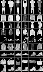
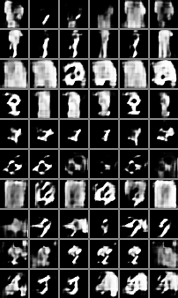
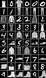
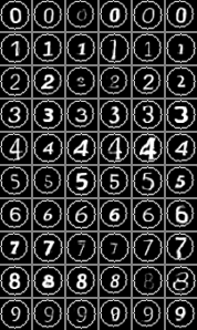
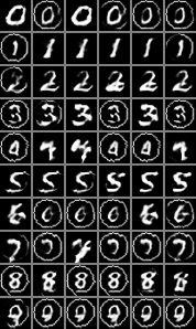
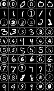
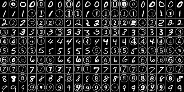
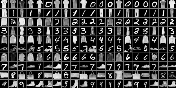
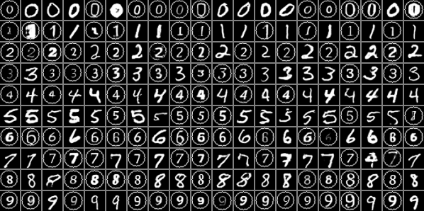
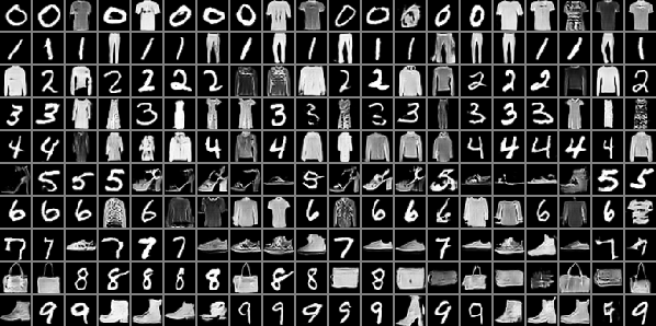
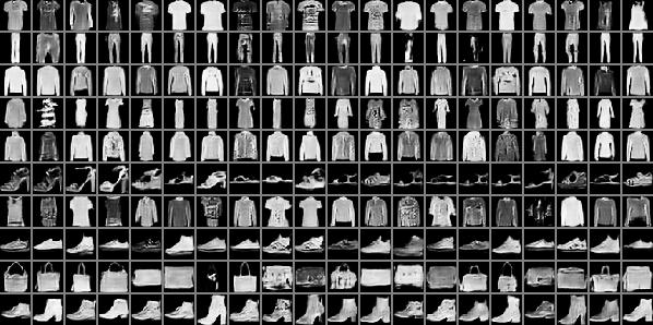
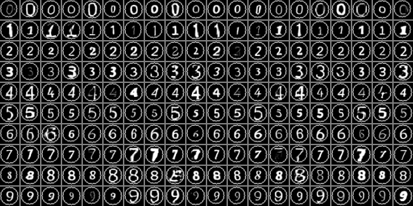
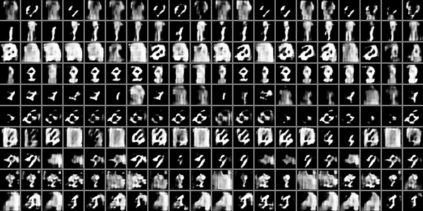
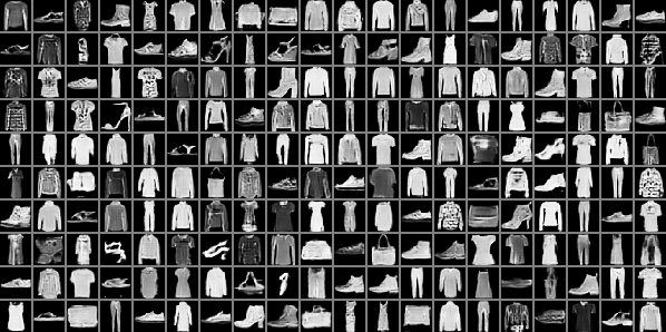
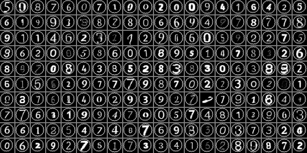
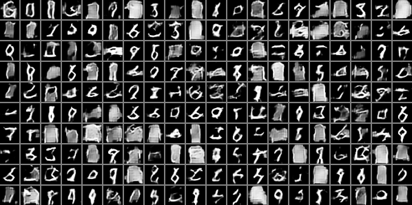
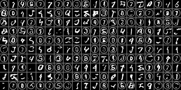
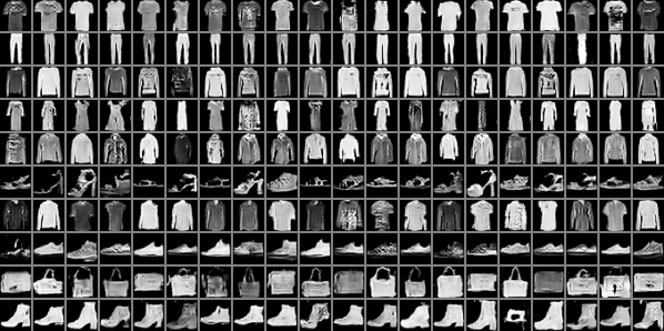
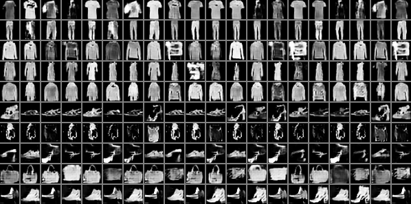
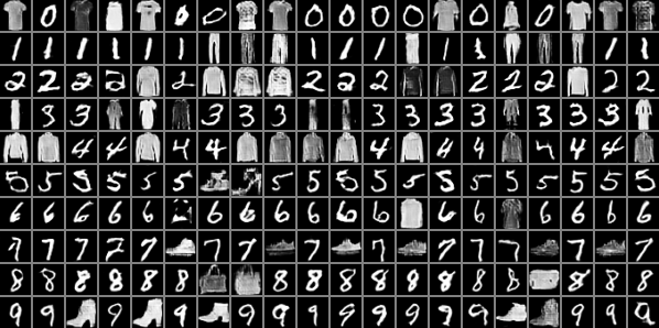
The superior performance of UA-GAN can be illustrated by qualitative examples in Fig. 3. On MNIST+Fashion dataset (subfigures a-c), the average aggregation strategy used by Avg-GAN could not effectively aggregate outputs of ‘non-identical’ local discriminators. Therefore, it only learns to generate the common patterns, e.g., Fashion images (Fig. 3(a)). MD-GAN fails to produce high quality images (Fig. 3(b)), probably because the discriminator switch makes the training not stable enough. Meanwhile, our UA-GAN is able to generate the mixture with both common patterns (Fashion images) and site-specific images (different digits from MNIST) with high quality. Similar phenomenon can be observed for MNIST+Font (subfigures d-f). Avg-GAN only learns the common pattern (computerized fonts from Font dataset), MD-GAN gives low quality images whereas UA-GAN can also learns the high-quality site-specific handwriting digits (MNIST).
Note that we also compare the methods on mixture datasets with i.i.d local distributions, i.e., all local datasets are sampled in a same way from the real datasets. In an i.i.d setting, all federated GANs and the centralized GAN perform similarly. More results will be included in the supplemental material.
(a) Avg GAN
(b) MD-GAN
(c) UA-GAN
(d) Avg GAN
(e) MD-GAN
(f) UA-GAN
5 Conclusion and Future Work
In this work, we proposed a provably correct federated GAN. It simulates a centralized discriminator via carefully aggregating the feedbacks of all local discriminators. We proved that the generator learns the target distribution. We also analyzed the error bound when the discriminator is suboptimal due to local dataset limitation. A well-trained federated GAN enpowers GANs to learn from diversified datasets. It can also be used as a data provider for training task-specific models without accessing or storing privacy sensitive data.
References
- [1] Dan Alistarh, Demjan Grubic, Jerry Li, Ryota Tomioka, and Milan Vojnovic. Qsgd: Communication-efficient sgd via gradient quantization and encoding. In Advances in Neural Information Processing Systems, pages 1709–1720, 2017.
- [2] George J Annas et al. Hipaa regulations-a new era of medical-record privacy? New England Journal of Medicine, 348(15):1486–1490, 2003.
- [3] Martin Arjovsky, Soumith Chintala, and Leon Bottou. Wasserstein gan. arXiv preprint arXiv:1701.07875, 2017.
- [4] Stephen Boyd and Lieven Vandenberghe. Convex optimization. Cambridge university press, 2004.
- [5] Imre Csiszar, Paul C Shields, et al. Information theory and statistics: A tutorial. Foundations and Trends® in Communications and Information Theory, 1(4):417–528, 2004.
- [6] Zihang Dai, Zhilin Yang, Fan Yang, William W Cohen, and Russ R Salakhutdinov. Good semi-supervised learning that requires a bad gan. In Advances in neural information processing systems, pages 6510–6520, 2017.
- [7] Ian Goodfellow, Jean Pouget-Abadie, Mehdi Mirza, Bing Xu, David Warde-Farley, Sherjil Ozair, Aaron Courville, and Yoshua Bengio. Generative adversarial nets. In Advances in neural information processing systems, pages 2672–2680, 2014.
- [8] Lawrence O Gostin, Laura A Levit, Sharyl J Nass, et al. Beyond the HIPAA privacy rule: enhancing privacy, improving health through research. National Academies Press, 2009.
- [9] Sudipto Guha, Piotr Indyk, and Andrew McGregor. Sketching information divergences. In International Conference on Computational Learning Theory (COLT), pages 424–438. Springer, 2007.
- [10] Ishaan Gulrajani, Faruk Ahmed, Martin Arjovsky, Vincent Dumoulin, and Aaron C Courville. Improved training of Wasserstein GANs. In Advances in Neural Information Processing Systems, 2017.
- [11] Corentin Hardy, Erwan Le Merrer, and Bruno Sericola. Md-gan: Multi-discriminator generative adversarial networks for distributed datasets. In 2019 IEEE International Parallel and Distributed Processing Symposium (IPDPS), pages 866–877. IEEE, 2019.
- [12] Kaiming He, Xiangyu Zhang, Shaoqing Ren, and Jian Sun. Deep residual learning for image recognition. In Proceedings of the IEEE conference on computer vision and pattern recognition, pages 770–778, 2016.
- [13] Kaiming He, Xiangyu Zhang, Shaoqing Ren, and Jian Sun. Deep Residual Learning for Image Recognition. 2016 IEEE Conference on Computer Vision and Pattern Recognition (CVPR), pages 770–778, 2016.
- [14] Martin Heusel, Hubert Ramsauer, Thomas Unterthiner, Bernhard Nessler, and Sepp Hochreiter. Gans trained by a two time-scale update rule converge to a local nash equilibrium. In Advances in neural information processing systems, pages 6626–6637, 2017.
- [15] Peter Kairouz, H Brendan McMahan, Brendan Avent, Aurelien Bellet, Mehdi Bennis, Arjun Nitin Bhagoji, Keith Bonawitz, Zachary Charles, Graham Cormode, Rachel Cummings, et al. Advances and open problems in federated learning. arXiv preprint arXiv:1912.04977, 2019.
- [16] Melita Sogomonjan1 Tanel Kerikmäe. Challenges in the e-health regulatory policy. HOW DEEP IS YOUR LAW? BREXIT. TECHNOLOGIES. MODERN CONFLICTS, 367, 2017.
- [17] Jakub Konecny, H Brendan McMahan, Felix X Yu, Peter Richtarik, Ananda Theertha Suresh, and Dave Bacon. Federated learning: Strategies for improving communication efficiency. arXiv preprint arXiv:1610.05492, 2016.
- [18] Abhishek Kumar, Prasanna Sattigeri, and Tom Fletcher. Semi-supervised learning with gans: Manifold invariance with improved inference. In Advances in Neural Information Processing Systems, pages 5534–5544, 2017.
- [19] Yann LeCun, Leon Bottou, Yoshua Bengio, and Patrick Haffner. Gradient-based learning applied to document recognition. Proceedings of the IEEE, 86(11):2278–2324, 1998.
- [20] Milieu Ltd & Time. lex. Overview of the national laws on electronic health records in the eu member states and their interaction with the provision of cross-border ehealth services: Final report and recommendations (contract 2013 63 02), viewed 18th march 2018. Communications of the ACM, 2014.
- [21] Xiang Li, Kaixuan Huang, Wenhao Yang, Shusen Wang, and Zhihua Zhang. On the convergence of fedavg on non-iid data. In International Conference on Learning Representations, 2020.
- [22] Xiang Li, Wenhao Yang, Shusen Wang, and Zhihua Zhang. Communication efficient decentralized training with multiple local updates. arXiv preprint arXiv:1910.09126, 2019.
- [23] Xiangru Lian, Ce Zhang, Huan Zhang, Cho-Jui Hsieh, Wei Zhang, and Ji Liu. Can decentralized algorithms outperform centralized algorithms? a case study for decentralized parallel stochastic gradient descent. In Advances in Neural Information Processing Systems, pages 5330–5340, 2017.
- [24] Jianhua Lin. Divergence measures based on the shannon entropy. IEEE Transactions on Information theory, 37(1):145–151, 1991.
- [25] Huidong Liu, Xianfeng Gu, and Dimitris Samaras. A two-step computation of the exact GAN Wasserstein distance. In Proceedings of the International Conference on Machine Learning, 2018.
- [26] Huidong Liu, Xianfeng Gu, and Dimitris Samaras. Wasserstein gan with quadratic transport cost. In The IEEE International Conference on Computer Vision (ICCV), October 2019.
- [27] Ming-Yu Liu, Xun Huang, Arun Mallya, Tero Karras, Timo Aila, Jaakko Lehtinen, and Jan Kautz. Few-shot unsupervised image-to-image translation. In Proceedings of the IEEE International Conference on Computer Vision, pages 10551–10560, 2019.
- [28] Brendan McMahan, Eider Moore, Daniel Ramage, Seth Hampson, and Blaise Aguera Y Arcas. Communication-efficient learning of deep networks from decentralized data. In Artificial Intelligence and Statistics, pages 1273–1282, 2017.
- [29] H Brendan McMahan, Eider Moore, Daniel Ramage, Seth Hampson, et al. Communication-efficient learning of deep networks from decentralized data. arXiv preprint arXiv:1602.05629, 2016.
- [30] Rebecca T Mercuri. The hipaa-potamus in health care data security. Communications of the ACM, 47(7):25–28, 2004.
- [31] Lars Mescheder, Andreas Geiger, and Sebastian Nowozin. Which training methods for gans do actually converge? In Proceedings of the International Conference on Machine Learning, 2018.
- [32] Mehdi Mirza and Simon Osindero. Conditional generative adversarial nets. arXiv preprint arXiv:1411.1784, 2014.
- [33] Takeru Miyato, Toshiki Kataoka, Masanori Koyama, and Yuichi Yoshida. Spectral normalization for generative adversarial networks. In Proceedings of the International Conference on Learning Representations, 2018.
- [34] Lawrence Mo. Internet-based font server, January 24 2002. US Patent App. 09/863,250.
- [35] Lam M Nguyen, Phuong Ha Nguyen, Marten van Dijk, Peter Richtarik, Katya Scheinberg, and Martin Takáč. Sgd and hogwild! convergence without the bounded gradients assumption. arXiv preprint arXiv:1802.03801, 2018.
- [36] Guo-Jun Qi. Loss-sensitive generative adversarial networks on lipschitz densities. International Journal of Computer Vision, pages 1–23, 2019.
- [37] Hui Qu, Yikai Zhang, Qi Chang, Zhennan Yan, Chao Chen, and Dimitris Metaxas. Learn distributed gan with temporary discriminators. arXiv preprint arXiv:2007.09221, 2020.
- [38] Benjamin Recht, Christopher Re, Stephen Wright, and Feng Niu. Hogwild: A lock-free approach to parallelizing stochastic gradient descent. In Advances in neural information processing systems, pages 693–701, 2011.
- [39] Tim Salimans, Ian Goodfellow, Wojciech Zaremba, Vicki Cheung, Alec Radford, and Xi Chen. Improved techniques for training GANs. In Advances in Neural Information Processing Systems, 2016.
- [40] Jonathan JM Seddon and Wendy L Currie. Cloud computing and trans-border health data: Unpacking us and eu healthcare regulation and compliance. Health policy and technology, 2(4):229–241, 2013.
- [41] Tamar Rott Shaham, Tali Dekel, and Tomer Michaeli. Singan: Learning a generative model from a single natural image. In Proceedings of the IEEE International Conference on Computer Vision, pages 4570–4580, 2019.
- [42] Karen Simonyan and Andrew Zisserman. Very deep convolutional networks for large-scale image recognition. arXiv preprint arXiv:1409.1556, 2014.
- [43] Virginia Smith, Chao-Kai Chiang, Maziar Sanjabi, and Ameet S Talwalkar. Federated multi-task learning. In Advances in Neural Information Processing Systems, pages 4424–4434, 2017.
- [44] Hoang Thanh-Tung, Truyen Tran, and Svetha Venkatesh. Improving generalization and stability of generative adversarial networks. In Proceedings of the International Conference on Learning Representations, 2019.
- [45] Kang Wei, Jun Li, Ming Ding, Chuan Ma, Howard H Yang, Farhad Farokhi, Shi Jin, Tony QS Quek, and H Vincent Poor. Federated learning with differential privacy: Algorithms and performance analysis. IEEE Transactions on Information Forensics and Security, 2020.
- [46] Han Xiao, Kashif Rasul, and Roland Vollgraf. Fashion-mnist: a novel image dataset for benchmarking machine learning algorithms. arXiv preprint arXiv:1708.07747, 2017.
- [47] Bangzhou Xin, Wei Yang, Yangyang Geng, Sheng Chen, Shaowei Wang, and Liusheng Huang. Private fl-gan: Differential privacy synthetic data generation based on federated learning. In ICASSP 2020-2020 IEEE International Conference on Acoustics, Speech and Signal Processing (ICASSP), pages 2927–2931. IEEE, 2020.
- [48] Qiang Yang, Yang Liu, Tianjian Chen, and Yongxin Tong. Federated machine learning: Concept and applications. ACM Transactions on Intelligent Systems and Technology (TIST), 10(2):1–19, 2019.
- [49] Hao Yu, Rong Jin, and Sen Yang. On the linear speedup analysis of communication efficient momentum sgd for distributed non-convex optimization. In International Conference on Machine Learning, pages 7184–7193, 2019.
- [50] Ruixiang Zhang, Tong Che, Zoubin Ghahramani, Yoshua Bengio, and Yangqiu Song. Metagan: An adversarial approach to few-shot learning. In Advances in Neural Information Processing Systems, pages 2365–2374, 2018.
- [51] Yue Zhao, Meng Li, Liangzhen Lai, Naveen Suda, Damon Civin, and Vikas Chandra. Federated learning with non-iid data. arXiv preprint arXiv:1806.00582, 2018.
- [52] Ligeng Zhu, Zhijian Liu, and Song Han. Deep leakage from gradients. In Advances in Neural Information Processing Systems 32, pages 14774–14784. Curran Associates, Inc., 2019.
In this supplemental material, we provide proofs of the theorems in the main paper (Sec. A). We also provide additional experimental details and results (Sec. B).
Appendix A Proofs of Theorems in Section 3
We recall the definition of odds value.
Definition 2 (odds value).
Given a probability , its odds value is . Note the definition requires .
A.1 Analysis of Optimal Discriminator
We recall the theorem of the correctness of UA-GAN.
Theorem 1 (Correctness).
Suppose all discriminators ’s are optimal. is computed via Eq. (11). The optimal distribution of the Jenson-Shannon divergence loss:
| (9) |
is where is the density (mass) function of .
To prove the theorem, we first introduce the following Lemma, which is similar to Proposition 1 in [7]. We include the Lemma and Proof here for completeness.
Lemma 1.
When generator is fixed, the optimal discriminator is :
| (10) |
Proof:
by setting we can maximize each component in the integral thus make the inequality hold with equality. ∎
Proof of Theorem 1:
Suppose in each training step the discriminator achieves its maximal criterion in Lemma 1, the simulated becomes:
| (11) |
Given that discriminators behave optimally, the value of which implies . By the aggregation formula 11, the simulated discriminator will be . Suppose in each training step the discriminator achieves its maximal criterion in Lemma 1, the loss function for the generator becomes:
The above loss function has optimal solution of due to Theorem 1 in [7]. ∎
A.2 Analysis of sub-optimal discriminator
Theorem 2 (Suboptimality Bound for a Single Discriminator).
Suppose a discriminator is a perturbed version of the optimal discriminator , s.t. with and . Let be the optimal distribution of the Jensen-Shannon divergence loss based on the perturbed discriminator
| (12) |
Then satisfies .
Lemma 2.
Suppose , with , we have .
Proof:
In the proof we will use following fact:
| (13) |
By equation we have thus:
| (14) | ||||
∎
Lemma 3.
Suppose , the following loss function is strongly convex:
| (15) |
Proof:
The first order derivative of is . The second order derivative is . (There is no non-diagonal elements in the Hessian). ∎
The proof for Theorem 2 is shown below. The theorem focuses on Jensen-Shannon Divergence loss [9, 24]. We stress that the analysis is general and works for both general GAN and conditional GAN.
Proof of Theorem 2:
Note . The perturbed odds value gives . Let , we have and
. The perturbed value of discriminator will be . The loss function that the generator distribution seeks to minimize a perturbed Jensen-Shannon Divergence loss:
| (16) |
where represents the Lagrangian Multiplier. In Lemma 3 we verify the convexity of this loss function with regulated behavior of . The derivative of w.r.t. is:
which needs to be for all value of [4]. Thus we have following equation:
| (17) |
Since above equation holds for all . Let which has value bounded by . we can multiply on both side and integral over :
which gives us where:
Plugging in above derived value of back into Equation 17 we have:
| (18) |
By the uniform upper bound on we have and . By taking exponential operation on both sides of Equation 18 we have :
Thus we can bound the value of by the equation:
| (19) |
. Due to the fact that the equation holds for all value of , by integrating Equation 19 we have which is equivalent to . Thus . By Lemma 2, we have . ∎
Theorem 3 (Tightness of the Bound in Theorem (2)).
Given a perturbed discriminator of the optimal one , s.t. with and . The optimal distribution as in Eq. (7) satisfies , .
Proof:
By similar steps to proof in Theorem 3 we have:
| (20) |
By setting the derivative of w.r.t. be we have :
| (21) |
Let . By assumption that we have
. Due to the fact that , we have . Thus we can bound .
Next we analyze following equation, we can multiply on both side of (17) and integral over :
which gives us where:
Plugging in above derived value of back into Equation 17 we have:
| (22) |
Next we analyze the term .
Due to the fact that , We can derive that . By an analysis similar to Theorem 3 we have . ∎
Corollary 1 (Suboptimality Bound for UA-GAN).
Assume suboptimal local discriminators are the perturbed versions of the optimal ones . And the suboptimality is bounded as: with , . The centralized discriminator is computed using these perturbed local discriminators such that . Let be the optimal distribution of the Jensen-Shannon divergence loss based on the perturbed UA discriminator
| (23) |
Then satisfies . In particular, the optimal distribution has total variation distance to the target distribution .
Proof:
Let ’s be odds values of optimal discriminators ’s: and ’s be odds values of suboptimal discriminators ’s. It suffices to show
and apply Theorem 2. ∎
Appendix B Additional Experimental Details and Results
(a) Avg GAN MNIST+Fashion
(b) Avg GAN MNIST+Font
(c) MD-GAN MNIST+Fashion
(d) MD-GAN MNIST+Font
(e) UA-GAN MNIST+Fashion
(f) UA-GAN MNIST+Font
Implementation Details:
Here we summarize details of the network we use in the experiments. Our UA-GAN has one centralized generator and multiple local discriminators. The generator consists of two fully-connected layers (for input noise and label, respectively), five residual blocks [13] and three upsampling layers. Each discriminator has two convolutional layers (for image and label, respectively), five residual blocks and three average pooling layers. LeakyReLU activation is used in both generator and discriminators. During training, we apply gradient update of the discriminators in each round. Each model is trained with Adam optimizer for 400 epochs with a batch size of 256. The learning rate is initially 0.0002 and linear decays to 0 from epoch 200. The VGG [42] 11-layer model is used for the downstream classification task. We pad the image to and then randomly crop them to with a batch size of 64 as input. The model is trained with SGD optimizer using a learning rate of 0.01 for 150 epochs.
Dataset Details:
One of our foundational datasets is the Font dataset. It is created from 2500+ fonts of digits taken from the Google Fonts database. Similar to MNIST, it consists of 10 classes of grayscale images, with 60k samples for training and 29k samples for test.
Based on the MNIST, Fashion-MNIST and Font dataset, we create both i.i.d mixture datasets and non-identical datasets. Details on non-identical datasets have been provided in the main paper. Here we provide details on two i.i.d datasets. (1) i.i.d MNIST+Fashion; (2) i.i.d MNIST+Font. Each of the 10 distributed sites contains 10% of mixture dataset which is uniformly sampled (without replacement) from MNIST and Fashion/Font.
B.1 Empirical Results on I.I.D. Datasets
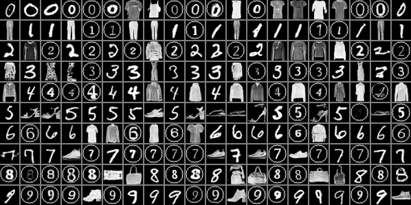
The quantitative results on the i.i.d mixture datasets are shown in Table 2. One can see all three distributed GAN methods have comparable performance. It can also be observed from qualitative examples in Fig. 4 that all three methods achieve similar results. This suggests that all three approaches can be used to train distributed GAN when datasets have i.i.d. distribution e.g., the data is uniformly shuffled before sent to each discriminator. Note that with a similar performance, the UA-GAN has much smaller communication cost compared to MD-GAN since the UA-GAN does not swap model parameters during training process.
| Dataset | i.i.d Mnist + Fashion | i.i.d Mnist + Font | ||||
| Accuracy | IS | FID | Accuracy | IS | FID | |
| Real | 0.943 | 3.620 0.021 | 0 | 0.994 | 2.323 0.011 | 0 |
| Centralized GAN | 0.904 | 3.437 0.021 | 8.35 | 0.979 | 1.978 0.009 | 17.62 |
| Avg GAN | 0.905 | 3.371 0.026 | 12.83 | 0.967 | 1.923 0.006 | 19.31 |
| MD-GAN | 0.884 | 3.364 0.024 | 13.63 | 0.971 | 1.938 0.008 | 19.65 |
| UA-GAN | 0.908 | 3.462 0.024 | 11.82 | 0.970 | 1.934 0.008 | 19.18 |
B.2 Additional Empirical Results on Non-identical Distribution
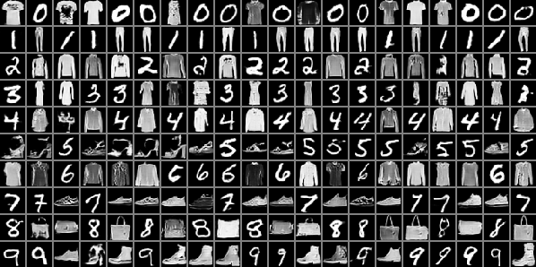
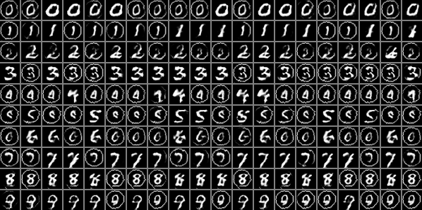
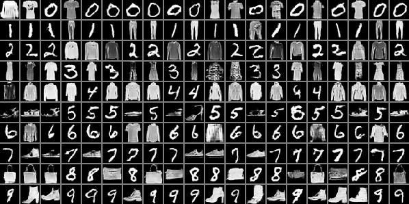
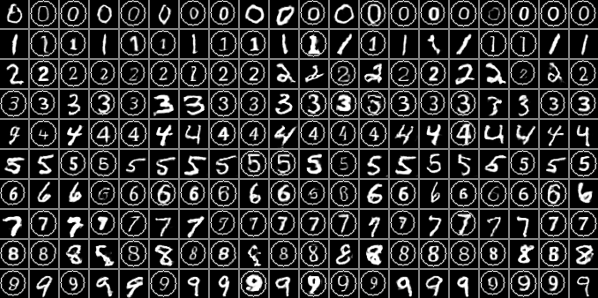
We provide additional synthetic images in non-identical distribution cases. See Fig. 5. By using average aggregation method, the synthetic image produced by Avg GAN and MD GAN only have Fashion images in (a), (c) and Font images in (b), (d). Our method in (e) and (f) could capture different patterns in MNIST + Fashion/Font and generate diverse images.
(a) Avg GAN MNIST+Fashion
(b) Avg GAN MNIST+Font
(c) MD-GAN MNIST+Fashion
(d) MD-GAN MNIST+Font
(e) UA-GAN MNIST+Fashion
(f) UA-GAN MNIST+Font
B.3 Empirical Results of Mixing Three Datasets
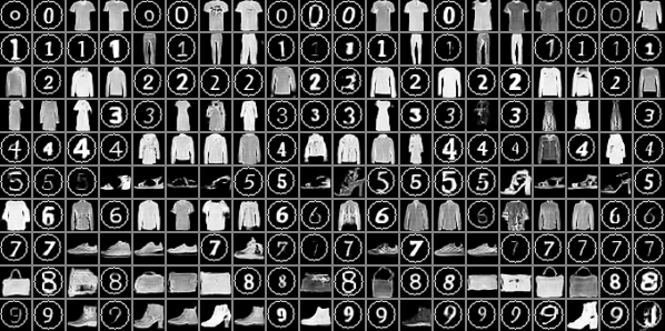
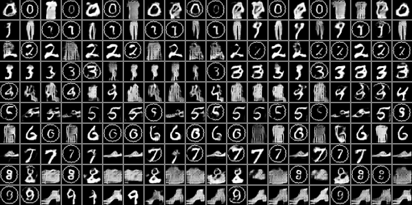
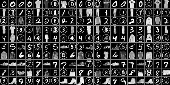
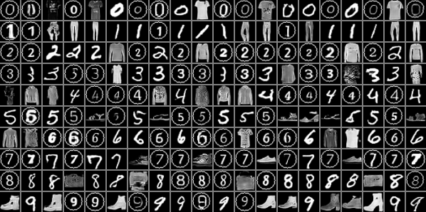
We report the results of mixing the three datasets MNIST, FashionMNIST and Font. In the non-identical setting, we add MNIST data with a distinct class among 09. These data are distinguishable features for different sites. And we uniformly sample Fashion and Font data for all 10 distributed sites. These are common patterns across all sites. In the identical setting, all three datasets are uniformly distributed across the 10 sites. The quantitative results are shown in Table 3. The synthtic images are shown in Fig. 6 and Fig. 7. By using average aggregation method, the synthetic image produced by Avg-GAN and MD -GAN only have Fashion and Font images in Fig. 6(a), (b) . Our method in Fig. 6(c) could capture different patterns in MNIST + Fashion + Font and generate diverse images.
| Dataset | non-i.i.d | i.i.d | ||||
| Accuracy | IS | FID | Accuracy | IS | FID | |
| Real | 0.955 | 3.426 0.023 | 0 | 0.955 | 3.426 0.023 | 0 |
| Centralized GAN | 0.943 | 3.031 0.016 | 14.90 | 0.943 | 3.031 0.016 | 14.90 |
| Avg GAN | 0.822 | 3.144 0.013 | 41.63 | 0.936 | 2.877 0.013 | 17.90 |
| MD-GAN | 0.567 | 3.035 0.011 | 56.19 | 0.936 | 2.951 0.019 | 16.81 |
| UA-GAN | 0.933 | 2.949 0.023 | 20.80 | 0.923 | 2.875 0.013 | 17.34 |
(a) Avg-GAN MNIST+Fashion+Font
(b) MD-GAN MNIST+Fashion+Font
(c) UA-GAN MNIST+Fashion+Font
(a) Avg-GAN MNIST+Fashion+Font
(b) MD-GAN MNIST+Fashion+Font
(c) UA-GAN MNIST+Fashion+Font
B.4 Empirical Results in larger federated learning setting
We report the results when using larger scale nodes() in distributed GAN methods(Avg-GAN, MD-GAN and UA-GAN). We uniformly split each individual site of the non-identical MNIST + Fashion dataset into 5 distributed sites. In total, we adopt non-identical MNIST+Fashion datasets with 2380 MNIST and Fashion images each. The quantitative results are shown in Table 4, and the synthetic images are shown in Fig 8.
| Dataset | non-i.i.d MNIST + Fashion (50 data sites) | ||
| Accuracy | IS | FID | |
| Real | 0.943 | 3.620 0.021 | 0 |
| Centralized GAN | 0.904 | 3.437 0.021 | 8.35 |
| Avg GAN | 0.489 | 3.755 0.023 | 90.36 |
| MD-GAN | 0.465 | 3.830 0.020 | 89.36 |
| UA-GAN | 0.626 | 3.531 0.018 | 53.26 |
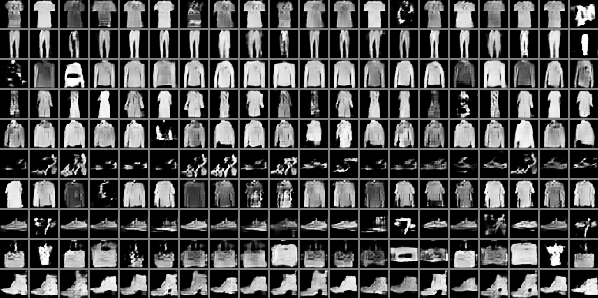
(a) Avg-GAN MNIST+Fashion(50 data sites)
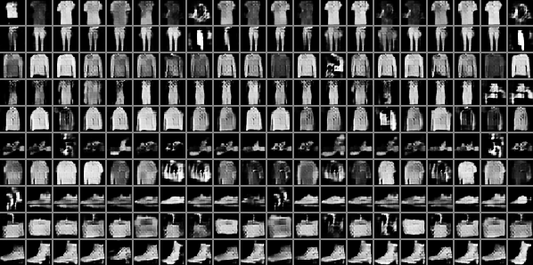
(b) MD-GAN MNIST+Fashion(50 data sites)
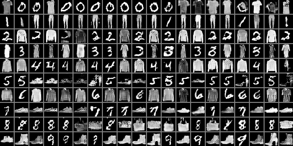
(c) UA-GAN MNIST+Fashion(50 data sites)
B.5 Empirical Results in unconditional setting
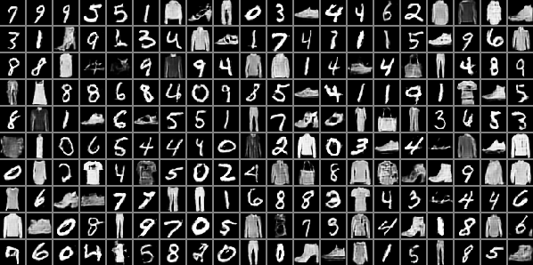
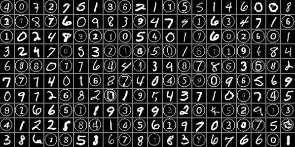
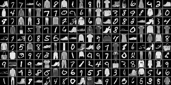
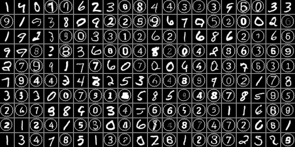
We report the results when using unconditional GAN in all methods (centralized, Avg-GAN, MD-GAN and UA-GAN). The quantitative results are shown in Table 5 and Table 6. The synthetic images are shown in Fig. 9 and Fig. 10. In the unconditional setting, the condition variable (labels) won’t be given thus one can not directly apply the synthetic data in training classification model. Therefore we don’t compute the classification accuracy in Table 5 and Table 6.
| Dataset | non-i.i.d MNIST + Fashion | non-i.i.d MNIST + Font | ||||
| Accuracy | IS | FID | Accuracy | IS | FID | |
| Real | 0.943 | 3.620 0.021 | 0 | 0.994 | 2.323 0.011 | 0 |
| Centralized GAN | - | 3.387 0.019 | 8.46 | - | 1.975 0.009 | 17.56 |
| Avg GAN | - | 4.068 0.020 | 61.56 | - | 1.547 0.005 | 80.07 |
| MD-GAN | - | 2.852 0.021 | 60.34 | - | 1.887 0.007 | 36.36 |
| UA-GAN | - | 3.280 0.022 | 22.34 | - | 1.985 0.013 | 22.17 |
| Dataset | i.i.d MNIST + Fashion | i.i.d MNIST + Font | ||||
| Accuracy | IS | FID | Accuracy | IS | FID | |
| Real | 0.943 | 3.620 0.021 | 0 | 0.994 | 2.323 0.011 | 0 |
| Centralized GAN | - | 3.387 0.019 | 8.46 | - | 1.975 0.009 | 17.56 |
| Avg GAN | - | 3.326 0.016 | 9.68 | - | 1.918 0.006 | 19.52 |
| MD-GAN | - | 3.428 0.025 | 12.04 | - | 1.934 0.006 | 18.85 |
| UA-GAN | - | 3.367 0.018 | 9.99 | - | 1.937 0.009 | 18.83 |
(a) Avg GAN MNIST+Fashion
(b) Avg GAN MNIST+Font
(c) MD-GAN MNIST+Fashion
(d) MD-GAN MNIST+Font
(e) UA-GAN MNIST+Fashion
(f) UA-GAN MNIST+Font
(a) Avg GAN MNIST+Fashion
(b) Avg GAN MNIST+Font
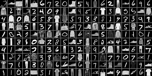
(c) MD-GAN MNIST+Fashion
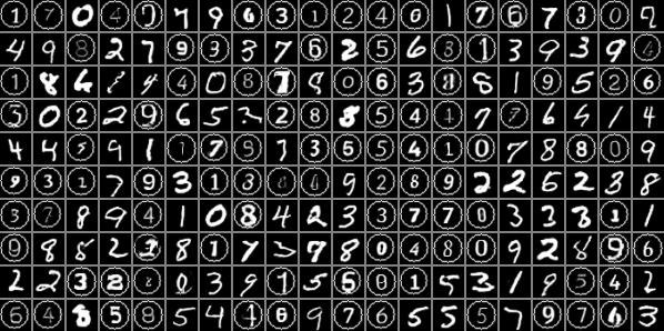
(d) MD-GAN MNIST+Font
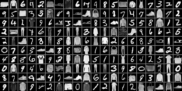
(e) UA-GAN MNIST+Fashion
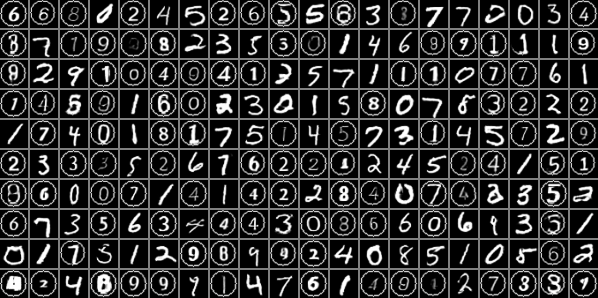
(f) UA-GAN MNIST+Font
B.6 Empirical results of imbalanced datasets in different sites
We report the results when the sizes of the 10 sites are not the same. Based on the non-identical MNIST + fashionMNIST dataset, we reduce the sample sizes of the first 5 sites by half and keep the other 5 sites unchanged. In this case, the numbers of images in each site are shown in Table 7. The quantitative results are shown in Table 8. The synthetic images are shown in Fig. 11.
| MNIST | 2917 | 3393 | 2944 | 3032 | 2939 | 5421 | 5918 | 6265 | 5851 | 5949 |
| Fashion | 3044 | 2978 | 3035 | 3033 | 2982 | 6000 | 6000 | 6000 | 6000 | 6000 |
| Total | 5961 | 6371 | 5979 | 6065 | 5921 | 11421 | 11918 | 12265 | 11851 | 11949 |
| Accuracy | IS | FID | |
| Real | 0.939 | 3.580 0.039 | 0 |
| Centralized GAN | 0.886 | 3.486 0.033 | 10.87 |
| Avg GAN | 0.497 | 3.809 0.025 | 74.45 |
| MD-GAN | 0.443 | 3.877 0.034 | 85.61 |
| UA-GAN | 0.846 | 2.717 0.019 | 30.30 |
(a) Avg-GAN MNIST+Fashion
(b) MD-GAN MNIST+Fashion
(c) UA-GAN MNIST+Fashion