Total Least Squares Phase Retrieval

Sidharth Gupta{}^{\,\dagger} and Ivan Dokmanić,{}^{\,\ddagger,\,\dagger}
{}^{\dagger}\,University of Illinois at Urbana-Champaign, {}^{\ddagger}\,University of Basel
gupta67@illinois.edu, ivan.dokmanic@unibas.ch
This work was supported by the European Research Council Starting Grant 852821—SWING.
Abstract

We address the phase retrieval problem with errors in the sensing vectors. A number of recent methods for phase retrieval are based on least squares (LS) formulations which assume errors in the quadratic measurements. We extend this approach to handle errors in the sensing vectors by adopting the total least squares (TLS) framework that is used in linear inverse problems with operator errors. We show how gradient descent and the specific geometry of the phase retrieval problem can be used to obtain a simple and efficient TLS solution. Additionally, we derive the gradients of the TLS and LS solutions with respect to the sensing vectors and measurements which enables us to calculate the solution errors. By analyzing these error expressions we determine conditions under which each method should outperform the other. We run simulations to demonstrate that our method can lead to more accurate solutions. We further demonstrate the effectiveness of our approach by performing phase retrieval experiments on real optical hardware which naturally contains both sensing vector and measurement errors.

Index Terms:
Phase retrieval, total least squares, operator error, sensing vector error, quadratic equations.

I Introduction

In the phase retrieval problem we seek to recover the signal 𝒙N𝒙superscript𝑁\bm{{x}}\in\mathbb{C}^{N} from complex quadratic measurements

ym|𝒂m,𝒙|2,m=1,,Mformulae-sequencesubscript𝑦𝑚superscriptsubscript𝒂𝑚𝒙2𝑚1𝑀\displaystyle y_{m}\approx{\left|\left\langle\bm{{a}}_{m},\bm{{x}}\right\rangle\right|}^{2},\qquad m=1,\ldots,M (1)

where ymsubscript𝑦𝑚y_{m}\in\mathbb{R} are observed measurements and 𝒂mNsubscript𝒂𝑚superscript𝑁\bm{{a}}_{m}\in\mathbb{C}^{N} are sensing vectors. This problem appears in a plethora of applied science applications such as x-ray diffraction crystallography or astronomy where the sensing vectors are Fourier basis vectors [1] and imaging through scattering media where the sensing vectors may be complex random Gaussian [2].

In a prototypical phase retrieval problem, an object, 𝒙𝒙\bm{{x}}, is illuminated and the resulting optical field is measured with a detector. This optical field is complex-valued but common camera sensors only measure intensity, {|𝒂m,𝒙|2}m=1Msuperscriptsubscriptsuperscriptsubscript𝒂𝑚𝒙2𝑚1𝑀\{{\left|\left\langle\bm{{a}}_{m},\bm{{x}}\right\rangle\right|}^{2}\}_{m=1}^{M}, and thus the measurement phase information is lost. The left and right hand sides in (1) are only approximately equal because in practical settings there can be errors in the measurements and sensing vectors. In this work we focus on gradient-based optimization strategies to solve (1) where M>N𝑀𝑁M>N. Gradient-based methods have proven successful when imaging through random scattering media [2] or with coded diffraction Fourier patterns [3].

Many recent approaches for solving the phase retrieval problem solve variants of the following nonlinear and nonconvex least squares (LS) problem,

min𝒙m=1M(ym|𝒂m,𝒙|2)2,subscript𝒙superscriptsubscript𝑚1𝑀superscriptsubscript𝑦𝑚superscriptsubscript𝒂𝑚𝒙22\displaystyle\min_{\bm{{x}}}\sum_{m=1}^{M}\left(y_{m}-{\left|\left\langle\bm{{a}}_{m},\bm{{x}}\right\rangle\right|}^{2}\right)^{2}, (LS-PR)

which we can alternatively rewrite as

min𝒙,r1,,rMsubscript𝒙subscript𝑟1subscript𝑟𝑀\displaystyle\min_{\begin{subarray}{c}\bm{{x}},\\ r_{1},\ldots,r_{M}\end{subarray}}\quad m=1Mrm2superscriptsubscript𝑚1𝑀superscriptsubscript𝑟𝑚2\displaystyle\sum_{m=1}^{M}r_{m}^{2} (2)
s.t. ym+rm=|𝒂m,𝒙|2,m=1,,Mformulae-sequencesubscript𝑦𝑚subscript𝑟𝑚superscriptsubscript𝒂𝑚𝒙2𝑚1𝑀\displaystyle y_{m}+r_{m}={\left|\left\langle\bm{{a}}_{m},\bm{{x}}\right\rangle\right|}^{2},\quad m=1,\ldots,M

with rmsubscript𝑟𝑚r_{m}\in\mathbb{R}. Thus, LS seeks the smallest correction to the measurements so that (ym+rm)subscript𝑦𝑚subscript𝑟𝑚(y_{m}+r_{m}) can be obtained from quadratic measurements |𝒂m,𝒙|2superscriptsubscript𝒂𝑚𝒙2{\left|\left\langle\bm{{a}}_{m},\bm{{x}}\right\rangle\right|}^{2} for each m𝑚m. This is analogous to LS for linear inverse problems where corrections that bring the measurements into the range space of the linear operator are required instead.

In many practical settings, the sensing vectors, {𝒂m}m=1Msuperscriptsubscriptsubscript𝒂𝑚𝑚1𝑀\{\bm{{a}}_{m}\}_{m=1}^{M}, are only approximately known via calibration. In this work we show that properly accounting for errors in the sensing vectors may lead to a more accurate estimate of 𝒙𝒙\bm{{x}}. Inspired by the total least squares (TLS) framework for linear [4, 5] and nonlinear [6] inverse problems, we extend the LS formulation (2) to find corrections for both the measurements and the sensing vectors. In TLS phase retrieval, we optimize the objective

min𝒙,r1,,rM,𝒆1,,𝒆Msubscript𝒙subscript𝑟1subscript𝑟𝑀subscript𝒆1subscript𝒆𝑀\displaystyle\min_{\begin{subarray}{c}\bm{{x}},\\ r_{1},\ldots,r_{M},\\ \bm{{e}}_{1},\ldots,\bm{{e}}_{M}\end{subarray}}\quad m=1Mλyrm2+λa𝒆m22superscriptsubscript𝑚1𝑀subscript𝜆𝑦superscriptsubscript𝑟𝑚2subscript𝜆𝑎superscriptsubscriptdelimited-∥∥subscript𝒆𝑚22\displaystyle\sum_{m=1}^{M}\lambda_{y}r_{m}^{2}+\lambda_{a}\left\lVert\bm{{e}}_{m}\right\rVert_{2}^{2} (3)
s.t. ym+rm=|𝒂m+𝒆m,𝒙|2,m=1,,Mformulae-sequencesubscript𝑦𝑚subscript𝑟𝑚superscriptsubscript𝒂𝑚subscript𝒆𝑚𝒙2𝑚1𝑀\displaystyle y_{m}+r_{m}={\left|\left\langle\bm{{a}}_{m}+\bm{{e}}_{m},\bm{{x}}\right\rangle\right|}^{2},\quad m=1,\ldots,M

with corrections 𝒆mNsubscript𝒆𝑚superscript𝑁\bm{{e}}_{m}\in\mathbb{C}^{N} for 1mM1𝑚𝑀1\leq m\leq M. Scalars λysubscript𝜆𝑦\lambda_{y}\in\mathbb{R} and λasubscript𝜆𝑎\lambda_{a}\in\mathbb{R} are nonnegative regularization weights. Now for each m𝑚m we want to find minimum weighted norm corrections so that (ym+rm)subscript𝑦𝑚subscript𝑟𝑚(y_{m}+r_{m}) can be obtained from quadratic measurements |𝒂m+𝒆m,𝒙|2superscriptsubscript𝒂𝑚subscript𝒆𝑚𝒙2{\left|\left\langle\bm{{a}}_{m}+\bm{{e}}_{m},\bm{{x}}\right\rangle\right|}^{2}. Efficiently obtaining the sensing vector corrections {𝒆m}m=1Msuperscriptsubscriptsubscript𝒆𝑚𝑚1𝑀\{\bm{{e}}_{m}\}_{m=1}^{M} is a major challenge when moving from the LS problem (2) to the TLS problem (3).

I-A Related work

Algorithms by Gerchberg and Saxton [7] and Fienup [8] are the most well-known approaches for solving the phase retrieval problem when the sensing vectors are the rows of the Fourier matrix, as in many practical imaging scenarios [9]. These methods iteratively reduce the error between the observed measurements and the measurements generated from the solution at the current iterate. Another class of algorithms based on message passing have also been developed [10, 11]. Despite the nonconvexity of the problem, these error reduction and message passing algorithms work well in practice. They do not directly use gradient descent to obtain a solution.

Recently a series of works have shown that for suitable measurement models, the nonconvex LS objective (LS-PR) can be globally optimized via gradient descent updates. The Wirtinger flow algorithm is one of the most well-known methods and proposes the framework comprising a spectral initialization followed by gradient descent updates [3]. Spectral initialization ensures that the iterates start in a convex basin near a global optimum when there are enough measurements in an error-free setting. This initialization was first proposed as part of the AltMinPhase algorithm [12]. Multiple works have extended this approach by modifying the initialization, gradient updates and objective for phase retrieval [13, 14], and other quadratic problems with sensing matrices rather than sensing vectors [15] like the unassigned distance geometry problem [16]. There are also extensions that incorporate signal priors such as sparsity [17, 18]. None of these gradient descent approaches, however, account for sensing vector or sensing matrix errors.

Another group of works have developed convex optimization approaches, which are closely related to low-rank matrix recovery techniques, for solving the phase retrieval problem [19]. These methods use the fact that the measurements in (1) can be expressed using the Frobenius matrix inner product, ym|𝒂m,𝒙|2=𝒙𝒂m𝒂m𝒙=𝒂m𝒂m,𝒙𝒙subscript𝑦𝑚superscriptsubscript𝒂𝑚𝒙2superscript𝒙subscript𝒂𝑚superscriptsubscript𝒂𝑚𝒙subscript𝒂𝑚superscriptsubscript𝒂𝑚𝒙superscript𝒙y_{m}\approx{\left|\left\langle\bm{{a}}_{m},\bm{{x}}\right\rangle\right|}^{2}=\bm{{x}}^{*}\bm{{a}}_{m}\bm{{a}}_{m}^{*}\bm{{x}}=\left\langle\bm{{a}}_{m}\bm{{a}}_{m}^{*},\bm{{x}}\bm{{x}}^{*}\right\rangle. With this formulation, phase retrieval amounts to recovering a rank-1 positive semidefinite matrix, 𝑿=𝒙𝒙𝑿𝒙superscript𝒙\bm{{X}}=\bm{{x}}\bm{{x}}^{*}, from linear matrix inner product measurements, {𝒂m𝒂m,𝒙𝒙}m=1Msuperscriptsubscriptsubscript𝒂𝑚superscriptsubscript𝒂𝑚𝒙superscript𝒙𝑚1𝑀\{\left\langle\bm{{a}}_{m}\bm{{a}}_{m}^{*},\bm{{x}}\bm{{x}}^{*}\right\rangle\}_{m=1}^{M} [20, 21]. In practice, lifting the problem from recovering vectors in Nsuperscript𝑁\mathbb{C}^{N} to matrices in N×Nsuperscript𝑁𝑁\mathbb{C}^{N\times N} poses significant computational and memory challenges for even moderately sized problems. Matrix sketching algorithms [22] and convex methods which do not require lifting [23] have since been developed to address these challenges.

For linear inverse problems, the TLS method is an established approach for handling errors in both the measurements and the operator [4, 5]. For linear problems, TLS can be efficiently solved using the singular value decomposition (SVD). For the quadratic case considered in this paper, such an approach is not apparent because of the magnitude-squared nonlinearity in (1). We therefore also cannot use the SVD to analyze the solution error as is done in the linear case [24]. Linear TLS has been extended to settings with structured operator errors [25, 26], sparse signals [27], and signals with norm constraints [28]. We note that Yagle and Bell use linear TLS to solve a particular subproblem in a phase retrieval algorithm which only addresses errors in the measurements [29].

There also exist algorithms for nonlinear TLS which aim to solve a general optimization problem for inverse problems with arbitrary nonlinearities [6, 30, 31]. The general optimization problem is similar to (3) except for the constraint which requires nonlinear rather than quadratic consistency. However, by using the specific structure of the phase retrieval problem (1) we are able to obtain efficient algorithms and perform error analysis for TLS phase retrieval.

Our gradient descent strategy uses alternating updates to solve the TLS phase retrieval problem. While alternating updates have been successfully utilized to solve the linear TLS problem [27], it is not straightforward to extend this approach to phase retrieval because of its quadratic nature. We show how to use the geometry of the optimization problem (3) to perform alternating updates for TLS phase retrieval.

I-B Contributions and paper organization

We propose a TLS framework for solving the phase retrieval problem when there are errors in the sensing vectors. In Section II we explain our gradient descent strategy to solve the TLS phase retrieval problem which motivates an alternating updates procedure to solve the problem. With this approach there are additional computational challenges which we show can be made efficient by incorporating the geometry of the phase retrieval problem. In Section III we derive expressions for the reconstruction errors for the TLS and LS solutions. This gives us insight into when each method should perform well. This derivation requires the usage of theorems about differentiation of argmins and different matrix inversion lemmas. Through simulations in Section IV we show that the TLS approach can lead to solutions of greater accuracy when there are sensing vector errors. We further verify the applicability of our framework through experiments on real optical hardware in Section V. We see that TLS outperforms LS when aiming to recover random signals and real images. We conclude and motivate future work in Section VI.

II TLS for phase retrieval

In this section we show how to solve the TLS phase retrieval problem. Recall (3),

min𝒙,r1,,rM,𝒆1,,𝒆Msubscript𝒙subscript𝑟1subscript𝑟𝑀subscript𝒆1subscript𝒆𝑀\displaystyle\min_{\begin{subarray}{c}\bm{{x}},\\ r_{1},\ldots,r_{M},\\ \bm{{e}}_{1},\ldots,\bm{{e}}_{M}\end{subarray}}\quad \mfrac12Mm=1Mλyrm2+λa𝒆m22,\mfrac12𝑀superscriptsubscript𝑚1𝑀subscript𝜆𝑦superscriptsubscript𝑟𝑚2subscript𝜆𝑎superscriptsubscriptdelimited-∥∥subscript𝒆𝑚22\displaystyle\mfrac{1}{2M}\sum_{m=1}^{M}\lambda_{y}r_{m}^{2}+\lambda_{a}\left\lVert\bm{{e}}_{m}\right\rVert_{2}^{2}, (4)
s.t. ym+rm=|𝒂m+𝒆m,𝒙|2,m=1,,M,formulae-sequencesubscript𝑦𝑚subscript𝑟𝑚superscriptsubscript𝒂𝑚subscript𝒆𝑚𝒙2𝑚1𝑀\displaystyle y_{m}+r_{m}={\left|\left\langle\bm{{a}}_{m}+\bm{{e}}_{m},\bm{{x}}\right\rangle\right|}^{2},\quad m=1,\ldots,M,

which has been normalized by the number of measurements by the scaling 1M1𝑀\frac{1}{M}. We can rearrange the constraint and substitute rm=|𝒂m+𝒆m,𝒙|2ymsubscript𝑟𝑚superscriptsubscript𝒂𝑚subscript𝒆𝑚𝒙2subscript𝑦𝑚r_{m}={\left|\left\langle\bm{{a}}_{m}+\bm{{e}}_{m},\bm{{x}}\right\rangle\right|}^{2}-y_{m} for 1mM1𝑚𝑀1\leq m\leq M to obtain,

min𝒙\mfrac12Mm=1Mmin𝒆mλa𝒆m22+λy(ym|𝒂m+𝒆m,𝒙|2)2.subscript𝒙\mfrac12𝑀superscriptsubscript𝑚1𝑀subscriptsubscript𝒆𝑚subscript𝜆𝑎superscriptsubscriptdelimited-∥∥subscript𝒆𝑚22subscript𝜆𝑦superscriptsubscript𝑦𝑚superscriptsubscript𝒂𝑚subscript𝒆𝑚𝒙22\displaystyle\min_{\bm{{x}}}\mfrac{1}{2M}\sum_{m=1}^{M}\min_{\bm{{e}}_{m}}\lambda_{a}\left\lVert\bm{{e}}_{m}\right\rVert_{2}^{2}+\lambda_{y}\left(y_{m}-{\left|\left\langle\bm{{a}}_{m}+\bm{{e}}_{m},\bm{{x}}\right\rangle\right|}^{2}\right)^{2}. (5)

Further we denote the m𝑚mth corrected sensing vector as 𝒂^m:=(𝒂m+𝒆m)assignsubscript^𝒂𝑚subscript𝒂𝑚subscript𝒆𝑚\widehat{\bm{{a}}}_{m}:=(\bm{{a}}_{m}+\bm{{e}}_{m}) to obtain the equivalent formulations

min𝒙\mfrac12Mm=1Mmin𝒂^mλa𝒂m𝒂^m22+λy(ym|𝒂^m,𝒙|2)2m(𝒙),subscript𝒙\mfrac12𝑀superscriptsubscript𝑚1𝑀subscriptsubscriptsubscript^𝒂𝑚subscript𝜆𝑎superscriptsubscriptdelimited-∥∥subscript𝒂𝑚subscript^𝒂𝑚22subscript𝜆𝑦superscriptsubscript𝑦𝑚superscriptsubscript^𝒂𝑚𝒙22subscript𝑚𝒙\displaystyle\min_{\bm{{x}}}\mfrac{1}{2M}\sum_{m=1}^{M}\underbrace{\min_{\widehat{\bm{{a}}}_{m}}\lambda_{a}\left\lVert\bm{{a}}_{m}-\widehat{\bm{{a}}}_{m}\right\rVert_{2}^{2}+\lambda_{y}\left(y_{m}-{\left|\left\langle\widehat{\bm{{a}}}_{m},\bm{{x}}\right\rangle\right|}^{2}\right)^{2}}_{\mathcal{I}_{m}(\bm{{x}})}, (TLS-PR1)

and

min𝒙,𝒂^1,,𝒂^M\mfrac12Mm=1Mλa𝒂m𝒂^m22+λy(ym|𝒂^m,𝒙|2)2𝒥(𝒙,𝒂^1,,𝒂^M).subscript𝒙subscript^𝒂1subscript^𝒂𝑀subscript\mfrac12𝑀superscriptsubscript𝑚1𝑀subscript𝜆𝑎superscriptsubscriptdelimited-∥∥subscript𝒂𝑚subscript^𝒂𝑚22subscript𝜆𝑦superscriptsubscript𝑦𝑚superscriptsubscript^𝒂𝑚𝒙22𝒥𝒙subscript^𝒂1subscript^𝒂𝑀\displaystyle\min_{\begin{subarray}{c}\bm{{x}},\\ \widehat{\bm{{a}}}_{1},\ldots,\widehat{\bm{{a}}}_{M}\end{subarray}}\underbrace{\mfrac{1}{2M}\sum_{m=1}^{M}\lambda_{a}\left\lVert\bm{{a}}_{m}-\widehat{\bm{{a}}}_{m}\right\rVert_{2}^{2}+\lambda_{y}\left(y_{m}-{\left|\left\langle\widehat{\bm{{a}}}_{m},\bm{{x}}\right\rangle\right|}^{2}\right)^{2}}_{\mathcal{J}(\bm{{x}},\widehat{\bm{{a}}}_{1},\ldots,\widehat{\bm{{a}}}_{M})}. (TLS-PR2)

As each data consistency term, (ym|𝒂^m,𝒙|2)2superscriptsubscript𝑦𝑚superscriptsubscript^𝒂𝑚𝒙22\left(y_{m}-{\left|\left\langle\widehat{\bm{{a}}}_{m},\bm{{x}}\right\rangle\right|}^{2}\right)^{2}, is proportional to 𝒙24superscriptsubscriptdelimited-∥∥𝒙24\left\lVert\bm{{x}}\right\rVert_{2}^{4} in an error-free setting, we set λy=λy𝒙(0)24subscript𝜆𝑦superscriptsubscript𝜆𝑦superscriptsubscriptdelimited-∥∥superscript𝒙024\lambda_{y}=\frac{\lambda_{y}^{\dagger}}{\left\lVert\bm{{x}}^{(0)}\right\rVert_{2}^{4}} in order to make the scaling of the objective invariant with respect to the norm of 𝒙𝒙\bm{{x}}. The vector 𝒙(0)superscript𝒙0\bm{{x}}^{(0)} is an initial guess for 𝒙𝒙\bm{{x}} and λysuperscriptsubscript𝜆𝑦\lambda_{y}^{\dagger} is a regularization parameter. Furthermore, to account for the fact that the sensing vector corrections, (𝒂m𝒂^m)subscript𝒂𝑚subscript^𝒂𝑚(\bm{{a}}_{m}-\widehat{\bm{{a}}}_{m}), are N𝑁N-dimensional and the data consistency terms are scalar we set λa=λaNsubscript𝜆𝑎superscriptsubscript𝜆𝑎𝑁\lambda_{a}=\frac{\lambda_{a}^{\dagger}}{N} where λasuperscriptsubscript𝜆𝑎\lambda_{a}^{\dagger} is a regularization parameter.

In line with recent methods such as the Wirtinger flow algorithm [3], our high level strategy is to obtain 𝒙𝒙\bm{{x}} by solving

argmin𝒙\mfrac12Mm=1Mm(𝒙),subscriptargmin𝒙\mfrac12𝑀superscriptsubscript𝑚1𝑀subscript𝑚𝒙\displaystyle\operatorname*{arg\,min}_{\bm{{x}}}\mfrac{1}{2M}\sum_{m=1}^{M}\mathcal{I}_{m}(\bm{{x}}), (6)

using gradient descent. To perform gradient descent with respect to 𝒙𝒙\bm{{x}} we can use Wirtinger gradient updates [3],

𝒙(τ+1)superscript𝒙𝜏1\displaystyle\bm{{x}}^{(\tau+1)} =𝒙(τ)\mfracμ𝒙(0)22\mfrac12Mm=1M𝒙m(𝒙(τ)),absentsuperscript𝒙𝜏\mfrac𝜇superscriptsubscriptdelimited-∥∥superscript𝒙022\mfrac12𝑀superscriptsubscript𝑚1𝑀subscript𝒙subscript𝑚superscript𝒙𝜏\displaystyle=\bm{{x}}^{(\tau)}-\mfrac{\mu}{\left\lVert\bm{{x}}^{(0)}\right\rVert_{2}^{2}}\cdot\mfrac{1}{2M}\sum_{m=1}^{M}\nabla_{\bm{{x}}}\mathcal{I}_{m}\left(\bm{{x}}^{(\tau)}\right), (7)

where μ𝜇\mu is the step size and 𝒙(0)2subscriptdelimited-∥∥superscript𝒙02\left\lVert\bm{{x}}^{(0)}\right\rVert_{2} is a guess for 𝒙2subscriptdelimited-∥∥𝒙2\left\lVert\bm{{x}}\right\rVert_{2}. The gradient is given by

𝒙m(𝒙)=2(|𝒂^m,𝒙|2ym)𝒂^m𝒂^m𝒙,subscript𝒙subscript𝑚𝒙2superscriptsuperscriptsubscript^𝒂𝑚𝒙2subscript𝑦𝑚superscriptsubscript^𝒂𝑚superscriptsubscript^𝒂𝑚absent𝒙\displaystyle\nabla_{\bm{{x}}}\mathcal{I}_{m}(\bm{{x}})=2\left({\left|\left\langle\widehat{\bm{{a}}}_{m}^{\dagger},\bm{{x}}\right\rangle\right|}^{2}-y_{m}\right)\widehat{\bm{{a}}}_{m}^{\dagger}\widehat{\bm{{a}}}_{m}^{{\dagger}*}\bm{{x}}, (8)

where 𝒂^msuperscriptsubscript^𝒂𝑚\widehat{\bm{{a}}}_{m}^{\dagger} is the solution to the following nonconvex optimization problem

𝒂^m=argmin𝒂λa𝒂m𝒂22+λy(ym|𝒂,𝒙|2)2.superscriptsubscript^𝒂𝑚subscriptargmin𝒂subscript𝜆𝑎superscriptsubscriptdelimited-∥∥subscript𝒂𝑚𝒂22subscript𝜆𝑦superscriptsubscript𝑦𝑚superscript𝒂𝒙22\displaystyle\widehat{\bm{{a}}}_{m}^{\dagger}=\operatorname*{arg\,min}_{\bm{{a}}}\lambda_{a}\left\lVert\bm{{a}}_{m}-\bm{{a}}\right\rVert_{2}^{2}+\lambda_{y}\left(y_{m}-{\left|\left\langle\bm{{a}},\bm{{x}}\right\rangle\right|}^{2}\right)^{2}. (9)

This motivates the following alternating updates procedure to solve the TLS problem:

  1. 1.

    Obtain an initial guess, 𝒙(0)Nsuperscript𝒙0superscript𝑁\bm{{x}}^{(0)}\in\mathbb{C}^{N}, for 𝒙𝒙\bm{{x}}.

  2. 2.

    Repeat steps 2a and 2b until convergence:

    1. (a)

      With 𝒙𝒙\bm{{x}} fixed, obtain corrected sensing vectors, {𝒂^m}m=1Msuperscriptsubscriptsuperscriptsubscript^𝒂𝑚𝑚1𝑀\{\widehat{\bm{{a}}}_{m}^{\dagger}\}_{m=1}^{M}, by solving (9) for 1mM1𝑚𝑀1\leq m\leq M.

    2. (b)

      With {𝒂^m}m=1Msuperscriptsubscriptsuperscriptsubscript^𝒂𝑚𝑚1𝑀\{\widehat{\bm{{a}}}_{m}^{\dagger}\}_{m=1}^{M} fixed, take one gradient descent step to update 𝒙𝒙\bm{{x}} using (7).

The main challenge in our approach is obtaining corrected sensing vectors {𝒂^m}m=1Msuperscriptsubscriptsuperscriptsubscript^𝒂𝑚𝑚1𝑀\{\widehat{\bm{{a}}}_{m}^{\dagger}\}_{m=1}^{M} by solving (9) so that we can perform gradient descent updates for 𝒙𝒙\bm{{x}} using (7). As (TLS-PR2) is nonconvex, a good initial guess, 𝒙(0)superscript𝒙0\bm{{x}}^{(0)}, can place us near a global minimum. There are multiple initialization options such as the spectral initialization for certain measurement models [12].

In the remainder of this section we will examine the geometry of the optimization problem in (TLS-PR1) and show how it can be leveraged to efficiently solve (9) and obtain corrected sensing vectors. This is summarized by Proposition 1 below. We will then present the complete TLS phase retrieval algorithm. Lastly, we also interpret the regularization parameters, λasubscript𝜆𝑎\lambda_{a} and λysubscript𝜆𝑦\lambda_{y}, by showing that the TLS solution is the maximum likelihood estimator for a quadratic complex-valued error-in-variables (EIV) model.

II-A Optimization geometry

Moving from the LS formulation to the TLS formulation introduces significant computational issues. In addition to optimizing over vector 𝒙𝒙\bm{{x}}, we must additionally optimize over M𝑀M sensing vectors in (TLS-PR1), with typically M>N𝑀𝑁M>N. We now study the optimization geometry of (TLS-PR1) and show that the M𝑀M inner minimizations over the N𝑁N-dimensional vectors, {𝒂^m}m=1Msuperscriptsubscriptsubscript^𝒂𝑚𝑚1𝑀\{\widehat{\bm{{a}}}_{m}\}_{m=1}^{M}, can be simplified to minimizing over M𝑀M scalars which improves efficiency. For ease of visualization in this subsection, we consider the real-valued problem (all quantities in (1), (LS-PR) and (TLS-PR1) are real) and we set λa=λy=1subscript𝜆𝑎subscript𝜆𝑦1\lambda_{a}=\lambda_{y}=1.

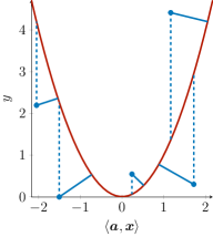
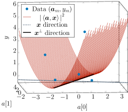
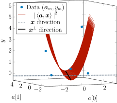
For a given vector 𝒙𝒙\bm{{x}} we compare the values of the LS and TLS objectives, (LS-PR) and (TLS-PR1). The left column of Fig. 1 visualizes the phase retrieval problem with M=5𝑀5M=5 data points, {(𝒂m,ym)}m=1Msuperscriptsubscriptsubscript𝒂𝑚subscript𝑦𝑚𝑚1𝑀\{(\bm{{a}}_{m},y_{m})\}_{m=1}^{M}, when N=2𝑁2N=2 and 𝒙2=1subscriptdelimited-∥∥𝒙21\left\lVert\bm{{x}}\right\rVert_{2}=1. The middle column shows the same data points from a different viewing angle. In phase retrieval we fit a paraboloid, y(𝒂)=|𝒂,𝒙|2𝑦𝒂superscript𝒂𝒙2y(\bm{{a}})={\left|\left\langle\bm{{a}},\bm{{x}}\right\rangle\right|}^{2} that is parameterized by 𝒙𝒙\bm{{x}} to the data points, {(𝒂m,ym)}m=1Msuperscriptsubscriptsubscript𝒂𝑚subscript𝑦𝑚𝑚1𝑀\{(\bm{{a}}_{m},y_{m})\}_{m=1}^{M}. If there is no sensing vector or measurement error, the data points lie on the paraboloid ((1) holds with equality). The left and middle figure show that the surface y(𝒂)=|𝒂,𝒙|2𝑦𝒂superscript𝒂𝒙2y(\bm{{a}})={\left|\left\langle\bm{{a}},\bm{{x}}\right\rangle\right|}^{2} does not change in the subspace perpendicular to 𝒙𝒙\bm{{x}}, denoted as 𝒙superscript𝒙perpendicular-to\bm{{x}}^{\perp}. This can also be verified by considering the values of 𝒂𝒂\bm{{a}} that would result in the inner product 𝒂,𝒙𝒂𝒙\left\langle\bm{{a}},\bm{{x}}\right\rangle being zero. Crucially this means that the shortest paths between the data points and the paraboloid have no component in the 𝒙superscript𝒙perpendicular-to\bm{{x}}^{\perp} subspace. As a result, we can view the problem in 2D from a viewpoint that looks into the 𝒙superscript𝒙perpendicular-to\bm{{x}}^{\perp} subspace as shown in the right column of Fig. 1. This 2D plot shows two options for measuring closeness between the surface and the data points. The LS objective (LS-PR), is the sum of the squared vertical distance between the 2D parabola and each data point as indicated by the dashed lines. On the other hand, due to the minima over all 𝒂^msubscript^𝒂𝑚\widehat{\bm{{a}}}_{m}, the TLS objective (TLS-PR1), is the sum of the squared Euclidean or orthogonal distance between the 2D parabola and each data point as shown by the solid lines. A similar geometrical interpretation is seen with linear TLS [4, 5].
Refer to caption
(a)
Refer to caption
(b)
Refer to caption
(c)
Figure 1: Visualization of the phase retrieval problem when 𝒙2=1subscriptdelimited-∥∥𝒙21\left\lVert\bm{{x}}\right\rVert_{2}=1. The left column shows M=5𝑀5M=5 data points, {(𝒂m,ym)}m=1Msuperscriptsubscriptsubscript𝒂𝑚subscript𝑦𝑚𝑚1𝑀\{(\bm{{a}}_{m},y_{m})\}_{m=1}^{M}, when N=2𝑁2N=2. A paraboloid is fitted to the data points. The middle column shows the same paraboloid and data points from a different viewing angle. The right column shows the problem from a viewpoint that looks into the 𝒙superscript𝒙perpendicular-to\bm{{x}}^{\perp} subspace. The dashed lines show the distances minimized by the LS objective, (LS-PR). The solid lines show the distances minimized by the TLS objective, (TLS-PR1).

Considering this geometry, to solve the inner minimizations in (TLS-PR1), we find the closest point on the paraboloid to each data point. As the shortest path has no component in the 𝒙superscript𝒙perpendicular-to\bm{{x}}^{\perp} subspace, our task of finding the closest point on a (N+1)𝑁1(N+1)-dimensional paraboloid to a (N+1)𝑁1(N+1)-dimensional data point reduces to a 2D geometry problem of finding the closest point on a parabola to a 2D data point. Rather than finding the minimizing N𝑁N-dimensional 𝒂^msuperscriptsubscript^𝒂𝑚\widehat{\bm{{a}}}_{m}^{\dagger} for each data point, we instead only need to find the component of 𝒂^msuperscriptsubscript^𝒂𝑚\widehat{\bm{{a}}}_{m}^{\dagger} in the 𝒙𝒙\bm{{x}} direction that is closest. This component is a scalar and is given by the inner product, νm=𝒂^m,𝒙subscript𝜈𝑚superscriptsubscript^𝒂𝑚𝒙\nu_{m}=\left\langle\widehat{\bm{{a}}}_{m}^{\dagger},\bm{{x}}\right\rangle. We can then construct 𝒂^msuperscriptsubscript^𝒂𝑚\widehat{\bm{{a}}}_{m}^{\dagger} by adding the unchanged component in the 𝒙superscript𝒙perpendicular-to\bm{{x}}^{\perp} subspace,

𝒂^m:=𝒂^m(νm)=νm𝒙2𝒙^+(𝒂m𝒂m,𝒙^𝒙^),assignsuperscriptsubscript^𝒂𝑚superscriptsubscript^𝒂𝑚subscript𝜈𝑚subscript𝜈𝑚subscriptdelimited-∥∥𝒙2^𝒙subscript𝒂𝑚subscript𝒂𝑚^𝒙^𝒙\displaystyle\widehat{\bm{{a}}}_{m}^{\dagger}:=\widehat{\bm{{a}}}_{m}^{\dagger}(\nu_{m})=\frac{\nu_{m}}{\left\lVert\bm{{x}}\right\rVert_{2}}\widehat{\bm{{x}}}+(\bm{{a}}_{m}-\left\langle\bm{{a}}_{m},\widehat{\bm{{x}}}\right\rangle\widehat{\bm{{x}}}), (10)

where 𝒙^^𝒙\widehat{\bm{{x}}} is 𝒙𝒙\bm{{x}} normalized.

If λasubscript𝜆𝑎\lambda_{a} and λysubscript𝜆𝑦\lambda_{y} are not one, a perpendicular distance is not minimized. As λaλysubscript𝜆𝑎subscript𝜆𝑦\frac{\lambda_{a}}{\lambda_{y}} gets larger, the solid lines in the right column of Fig. 1 become more vertical because there is a relatively larger penalty for correcting the sensing vectors and the problem moves towards a LS approach. Conversely, the lines become more horizontal as λaλysubscript𝜆𝑎subscript𝜆𝑦\frac{\lambda_{a}}{\lambda_{y}} gets smaller. Irrespective of the values of λasubscript𝜆𝑎\lambda_{a} and λysubscript𝜆𝑦\lambda_{y}, the shortest paths between the paraboloid and the data points still have no component in the 𝒙superscript𝒙perpendicular-to\bm{{x}}^{\perp} subspace and (10) can be used to obtain each 𝒂^msuperscriptsubscript^𝒂𝑚\widehat{\bm{{a}}}_{m}^{\dagger}. We further note that this geometry also holds for the complex-valued phase retrieval problem (1).

II-B Correcting complex-valued sensing vectors

Our strategy is to set up each inner minimization over 𝒂^msubscript^𝒂𝑚\widehat{\bm{{a}}}_{m} in (TLS-PR1) as the minimization of a fourth degree equation with respect to scalar νm=𝒂^m,𝒙subscript𝜈𝑚subscript^𝒂𝑚𝒙\nu_{m}=\left\langle\widehat{\bm{{a}}}_{m},\bm{{x}}\right\rangle rather than vector 𝒂^msubscript^𝒂𝑚\widehat{\bm{{a}}}_{m}. We then directly obtain the minimizer of this equation.

The M𝑀M inner minimization problems in (TLS-PR1) are independent of each other and we can independently solve each summand for a fixed vector 𝒙𝒙\bm{{x}}. Consider the objective function of optimization problem m(𝒙)subscript𝑚𝒙\mathcal{I}_{m}(\bm{{x}}),

fm(𝒂^m)=subscript𝑓𝑚subscript^𝒂𝑚absent\displaystyle f_{m}(\widehat{\bm{{a}}}_{m})= λa𝒂m𝒂^m22+λy(ym|𝒙𝒂^m|2)2.subscript𝜆𝑎superscriptsubscriptdelimited-∥∥subscript𝒂𝑚subscript^𝒂𝑚22subscript𝜆𝑦superscriptsubscript𝑦𝑚superscriptsuperscript𝒙subscript^𝒂𝑚22\displaystyle\lambda_{a}\left\lVert\bm{{a}}_{m}-\widehat{\bm{{a}}}_{m}\right\rVert_{2}^{2}+\lambda_{y}\left(y_{m}-{\left|\bm{{x}}^{*}\widehat{\bm{{a}}}_{m}\right|}^{2}\right)^{2}. (11)

Proposition 1 states that argmin𝒂^mfm(𝒂^m)subscriptargminsubscript^𝒂𝑚subscript𝑓𝑚subscript^𝒂𝑚\operatorname*{arg\,min}_{\widehat{\bm{{a}}}_{m}}f_{m}(\widehat{\bm{{a}}}_{m}) can be obtained by solving two scalar variable cubic equations and using (10).

Proposition 1.

Let sets R+subscript𝑅R_{+} and Rsubscript𝑅R_{-} be the positive real solutions of

αr3+βr±|γ|=0plus-or-minus𝛼superscript𝑟3𝛽𝑟𝛾0\displaystyle\alpha r^{3}+\beta r\pm{\left|\gamma\right|}=0 (12)

where α=2λy𝐱22𝛼2subscript𝜆𝑦superscriptsubscriptdelimited-∥∥𝐱22\alpha=2\lambda_{y}\left\lVert\bm{{x}}\right\rVert_{2}^{2}\in\mathbb{R}, β=λa2λyym𝐱22𝛽subscript𝜆𝑎2subscript𝜆𝑦subscript𝑦𝑚superscriptsubscriptdelimited-∥∥𝐱22\beta=\lambda_{a}-2\lambda_{y}y_{m}\left\lVert\bm{{x}}\right\rVert_{2}^{2}\in\mathbb{R} and γ=λa𝐱𝐚m𝛾subscript𝜆𝑎superscript𝐱subscript𝐚𝑚\gamma=-\lambda_{a}\bm{{x}}^{*}\bm{{a}}_{m}\in\mathbb{C}. Further, with κ𝜅\kappa denoting the phase of γ𝛾\gamma, let

S+={ejκr|rR+}andS={ejκr|rR}.subscript𝑆conditional-setsuperscripte𝑗𝜅𝑟𝑟subscript𝑅andsubscript𝑆conditional-setsuperscripte𝑗𝜅𝑟𝑟subscript𝑅\displaystyle S_{+}=\{\mathrm{e}^{j\kappa}r\,|\,r\in R_{+}\}\,\,\,\text{and}\,\,\,S_{-}=\{-\mathrm{e}^{j\kappa}r\,|\,r\in R_{-}\}. (13)

Then fm(𝐚^m)subscript𝑓𝑚subscript^𝐚𝑚f_{m}(\widehat{\bm{{a}}}_{m}) is minimized by 𝐚^m(s)superscriptsubscript^𝐚𝑚superscript𝑠\widehat{\bm{{a}}}_{m}^{\dagger}\left(s^{\dagger}\right) where

s=argminsS+Sfm(𝒂^m(s))superscript𝑠subscriptargmin𝑠subscript𝑆subscript𝑆subscript𝑓𝑚superscriptsubscript^𝒂𝑚𝑠\displaystyle s^{\dagger}=\operatorname*{arg\,min}_{s\in S_{+}\cup\,S_{-}}f_{m}\left(\widehat{\bm{{a}}}_{m}^{\dagger}(s)\right) (14)

and 𝐚^m()superscriptsubscript^𝐚𝑚\widehat{\bm{{a}}}_{m}^{\dagger}(\cdot) is defined in (10).

Proof:

Expanding fm(𝒂^m)subscript𝑓𝑚subscript^𝒂𝑚f_{m}(\widehat{\bm{{a}}}_{m}) gives

fm(𝒂^m)=subscript𝑓𝑚subscript^𝒂𝑚absent\displaystyle f_{m}(\widehat{\bm{{a}}}_{m})= λa(𝒂m22𝒂m𝒂^m𝒂^m𝒂m+𝒂^m𝒂^m)subscript𝜆𝑎superscriptsubscriptdelimited-∥∥subscript𝒂𝑚22superscriptsubscript𝒂𝑚subscript^𝒂𝑚superscriptsubscript^𝒂𝑚subscript𝒂𝑚superscriptsubscript^𝒂𝑚subscript^𝒂𝑚\displaystyle\lambda_{a}(\left\lVert\bm{{a}}_{m}\right\rVert_{2}^{2}-\bm{{a}}_{m}^{*}\widehat{\bm{{a}}}_{m}-\widehat{\bm{{a}}}_{m}^{*}\bm{{a}}_{m}+\widehat{\bm{{a}}}_{m}^{*}\widehat{\bm{{a}}}_{m})
+λy(ym22ym𝒂^m𝒙𝒙𝒂^m+(𝒂^m𝒙𝒙𝒂^m)2).subscript𝜆𝑦superscriptsubscript𝑦𝑚22subscript𝑦𝑚superscriptsubscript^𝒂𝑚𝒙superscript𝒙subscript^𝒂𝑚superscriptsuperscriptsubscript^𝒂𝑚𝒙superscript𝒙subscript^𝒂𝑚2\displaystyle+\lambda_{y}(y_{m}^{2}-2y_{m}\widehat{\bm{{a}}}_{m}^{*}\bm{{x}}\bm{{x}}^{*}\widehat{\bm{{a}}}_{m}+(\widehat{\bm{{a}}}_{m}^{*}\bm{{x}}\bm{{x}}^{*}\widehat{\bm{{a}}}_{m})^{2}). (15)

We can use Wirtinger derivatives to calculate the derivative of the real-valued fm(𝒂^m)subscript𝑓𝑚subscript^𝒂𝑚f_{m}(\widehat{\bm{{a}}}_{m}) with respect to the complex vector 𝒂^msubscript^𝒂𝑚\widehat{\bm{{a}}}_{m} [3],

𝒂^mfm=subscriptsubscript^𝒂𝑚subscript𝑓𝑚absent\displaystyle\nabla_{\widehat{\bm{{a}}}_{m}}f_{m}= (λa(𝒂m+𝒂^m)\displaystyle\left(\vphantom{{\left|\bm{{x}}^{*}\widehat{\bm{{a}}}_{m}\right|}^{2}}\lambda_{a}(-\bm{{a}}_{m}^{*}+\widehat{\bm{{a}}}_{m}^{*})\right.
+λy(2ym𝒂^m𝒙𝒙+2|𝒙𝒂^m|2𝒂^m𝒙𝒙))\displaystyle\left.+\lambda_{y}(-2y_{m}\widehat{\bm{{a}}}_{m}^{*}\bm{{x}}\bm{{x}}^{*}+2{\left|\bm{{x}}^{*}\widehat{\bm{{a}}}_{m}\right|}^{2}\widehat{\bm{{a}}}_{m}^{*}\bm{{x}}\bm{{x}}^{*})\right)^{*}
=\displaystyle= λa(𝒂^m𝒂m)subscript𝜆𝑎subscript^𝒂𝑚subscript𝒂𝑚\displaystyle\lambda_{a}(\widehat{\bm{{a}}}_{m}-\bm{{a}}_{m})
+λy(2ym𝒙𝒙𝒂^m+2|𝒙𝒂^m|2𝒙𝒙𝒂^m).subscript𝜆𝑦2subscript𝑦𝑚𝒙superscript𝒙subscript^𝒂𝑚2superscriptsuperscript𝒙subscript^𝒂𝑚2𝒙superscript𝒙subscript^𝒂𝑚\displaystyle+\lambda_{y}(-2y_{m}\bm{{x}}\bm{{x}}^{*}\widehat{\bm{{a}}}_{m}+2{\left|\bm{{x}}^{*}\widehat{\bm{{a}}}_{m}\right|}^{2}\bm{{x}}\bm{{x}}^{*}\widehat{\bm{{a}}}_{m}). (16)

Setting the derivative to zero, and then left-multiplying by nonzero 𝒙superscript𝒙\bm{{x}}^{*} gives

2λy𝒙22|𝒙𝒂^m|2(𝒙𝒂^m)2subscript𝜆𝑦superscriptsubscriptdelimited-∥∥𝒙22superscriptsuperscript𝒙subscript^𝒂𝑚2superscript𝒙subscript^𝒂𝑚\displaystyle 2\lambda_{y}\left\lVert\bm{{x}}\right\rVert_{2}^{2}{\left|\bm{{x}}^{*}\widehat{\bm{{a}}}_{m}\right|}^{2}(\bm{{x}}^{*}\widehat{\bm{{a}}}_{m}) 2λyym𝒙22(𝒙𝒂^m)2subscript𝜆𝑦subscript𝑦𝑚superscriptsubscriptdelimited-∥∥𝒙22superscript𝒙subscript^𝒂𝑚\displaystyle-2\lambda_{y}y_{m}\left\lVert\bm{{x}}\right\rVert_{2}^{2}(\bm{{x}}^{*}\widehat{\bm{{a}}}_{m})
+λa(𝒙𝒂^m)λa𝒙𝒂m=0subscript𝜆𝑎superscript𝒙subscript^𝒂𝑚subscript𝜆𝑎superscript𝒙subscript𝒂𝑚0\displaystyle+\lambda_{a}(\bm{{x}}^{*}\widehat{\bm{{a}}}_{m})-\lambda_{a}\bm{{x}}^{*}\bm{{a}}_{m}=0
2λy𝒙22|𝒙𝒂^m|2(𝒙𝒂^m)2subscript𝜆𝑦superscriptsubscriptdelimited-∥∥𝒙22superscriptsuperscript𝒙subscript^𝒂𝑚2superscript𝒙subscript^𝒂𝑚\displaystyle 2\lambda_{y}\left\lVert\bm{{x}}\right\rVert_{2}^{2}{\left|\bm{{x}}^{*}\widehat{\bm{{a}}}_{m}\right|}^{2}(\bm{{x}}^{*}\widehat{\bm{{a}}}_{m}) +(λa2λyym𝒙22)(𝒙𝒂^m)subscript𝜆𝑎2subscript𝜆𝑦subscript𝑦𝑚superscriptsubscriptdelimited-∥∥𝒙22superscript𝒙subscript^𝒂𝑚\displaystyle+(\lambda_{a}-2\lambda_{y}y_{m}\left\lVert\bm{{x}}\right\rVert_{2}^{2})(\bm{{x}}^{*}\widehat{\bm{{a}}}_{m})
λa𝒙𝒂m=0.subscript𝜆𝑎superscript𝒙subscript𝒂𝑚0\displaystyle-\lambda_{a}\bm{{x}}^{*}\bm{{a}}_{m}=0. (17)

The left hand side is now scalar-valued and is a function of scalar νm=𝒂^m,𝒙=𝒙𝒂^msubscript𝜈𝑚subscript^𝒂𝑚𝒙superscript𝒙subscript^𝒂𝑚\nu_{m}=\left\langle\widehat{\bm{{a}}}_{m},\bm{{x}}\right\rangle=\bm{{x}}^{*}\widehat{\bm{{a}}}_{m}\in\mathbb{C} instead of a vector. Recalling our analysis of the optimization geometry in Section II-A, we can solve for νmsubscript𝜈𝑚\nu_{m} and then obtain 𝒂^m=𝒂^m(νm)superscriptsubscript^𝒂𝑚superscriptsubscript^𝒂𝑚subscript𝜈𝑚\widehat{\bm{{a}}}_{m}^{\dagger}=\widehat{\bm{{a}}}_{m}^{\dagger}(\nu_{m}) using (10). If we substitute α=2λy𝒙22𝛼2subscript𝜆𝑦superscriptsubscriptdelimited-∥∥𝒙22\alpha=2\lambda_{y}\left\lVert\bm{{x}}\right\rVert_{2}^{2}\in\mathbb{R}, β=λa2λyym𝒙22𝛽subscript𝜆𝑎2subscript𝜆𝑦subscript𝑦𝑚superscriptsubscriptdelimited-∥∥𝒙22\beta=\lambda_{a}-2\lambda_{y}y_{m}\left\lVert\bm{{x}}\right\rVert_{2}^{2}\in\mathbb{R} and γ=λa𝒙𝒂m𝛾subscript𝜆𝑎superscript𝒙subscript𝒂𝑚\gamma=-\lambda_{a}\bm{{x}}^{*}\bm{{a}}_{m}\in\mathbb{C} we wish to solve the following for νmsubscript𝜈𝑚\nu_{m},

α|νm|2νm+βνm+γ=0.𝛼superscriptsubscript𝜈𝑚2subscript𝜈𝑚𝛽subscript𝜈𝑚𝛾0\displaystyle\alpha{\left|\nu_{m}\right|}^{2}\nu_{m}+\beta\nu_{m}+\gamma=0. (18)

Because the sensing vectors and ground truth signal are complex, this cubic equation is a function of νmsubscript𝜈𝑚\nu_{m}\in\mathbb{C} and its conjugate ν¯msubscript¯𝜈𝑚\bar{\nu}_{m} (|νm|2=νmν¯msuperscriptsubscript𝜈𝑚2subscript𝜈𝑚subscript¯𝜈𝑚{\left|\nu_{m}\right|}^{2}=\nu_{m}\bar{\nu}_{m}). We therefore cannot use standard cubic root finding formulae. Further note that the coefficients α𝛼\alpha and β𝛽\beta are always real and γ𝛾\gamma may be complex. To solve, first multiply by ν¯msubscript¯𝜈𝑚\bar{\nu}_{m},

α|νm|4+β|νm|2+γν¯m=0.𝛼superscriptsubscript𝜈𝑚4𝛽superscriptsubscript𝜈𝑚2𝛾subscript¯𝜈𝑚0\displaystyle\alpha{\left|\nu_{m}\right|}^{4}+\beta{\left|\nu_{m}\right|}^{2}+\gamma\bar{\nu}_{m}=0. (19)

Next, with complex-exponential representation, νm=rejϕsubscript𝜈𝑚𝑟superscripte𝑗italic-ϕ\nu_{m}=r\mathrm{e}^{j\phi} and γ=|γ|ejκ𝛾𝛾superscripte𝑗𝜅\gamma={\left|\gamma\right|}\mathrm{e}^{j\kappa} (recall γ𝛾\gamma is known), the equation becomes

αr3+βr+|γ|ej(κϕ)𝛼superscript𝑟3𝛽𝑟𝛾superscripte𝑗𝜅italic-ϕ\displaystyle\alpha r^{3}+\beta r+{\left|\gamma\right|}\mathrm{e}^{j(\kappa-\phi)} =0.absent0\displaystyle=0. (20)

The real and imaginary parts of the left hand side should both equate to zero. Using Euler’s identity, ejθ=cos(θ)+jsin(θ)superscripte𝑗𝜃𝜃𝑗𝜃\mathrm{e}^{j\theta}=\cos(\theta)+j\sin(\theta), we arrive at the following simultaneous equations,

{sin(κϕ)=0αr3+βr+|γ|cos(κϕ)=0.cases𝜅italic-ϕ0otherwise𝛼superscript𝑟3𝛽𝑟𝛾𝜅italic-ϕ0otherwise\begin{cases}\sin(\kappa-\phi)=0\\ \alpha r^{3}+\beta r+{\left|\gamma\right|}\cos(\kappa-\phi)=0.\end{cases} (21)

For the first equation to hold, cos(κϕ)=±1𝜅italic-ϕplus-or-minus1\cos(\kappa-\phi)=\pm 1 and so the phase of νmsubscript𝜈𝑚\nu_{m} has two possible values; ϕ=κitalic-ϕ𝜅\phi=\kappa or ϕ=(κπ)italic-ϕ𝜅𝜋\phi=(\kappa-\pi). To obtain the magnitude of νmsubscript𝜈𝑚\nu_{m} we can solve the following two cubic equations for r𝑟r to get six values, three from each,

αr3+βr+|γ|𝛼superscript𝑟3𝛽𝑟𝛾\displaystyle\alpha r^{3}+\beta r+{\left|\gamma\right|} =0andϕ=κformulae-sequenceabsent0anditalic-ϕ𝜅\displaystyle=0\quad\text{and}\quad\phi=\kappa (22)
αr3+βr|γ|𝛼superscript𝑟3𝛽𝑟𝛾\displaystyle\alpha r^{3}+\beta r-{\left|\gamma\right|} =0andϕ=κπ.formulae-sequenceabsent0anditalic-ϕ𝜅𝜋\displaystyle=0\quad\text{and}\quad\phi=\kappa-\pi. (23)

As the solutions of these two cubic equations are magnitudes of complex numbers, we let sets R+subscript𝑅R_{+} and Rsubscript𝑅R_{-} be the positive real solutions of (22) and (23) respectively. To obtain values for νmsubscript𝜈𝑚\nu_{m} we combine R+subscript𝑅R_{+} and Rsubscript𝑅R_{-} with their phases to get S+subscript𝑆S_{+} and Ssubscript𝑆S_{-}—multiply the elements of R+subscript𝑅R_{+} by ejκsuperscripte𝑗𝜅\mathrm{e}^{j\kappa} and multiply the elements of Rsubscript𝑅R_{-} by ej(κπ)=ejκsuperscripte𝑗𝜅𝜋superscripte𝑗𝜅\mathrm{e}^{j(\kappa-\pi)}=-\mathrm{e}^{j\kappa}. We then construct candidate minimizers of fm()subscript𝑓𝑚f_{m}(\cdot) by using the possible values for νmsubscript𝜈𝑚\nu_{m}, the set, S+Ssubscript𝑆subscript𝑆S_{+}\cup\,S_{-}, as the argument for (10). Finally, the global minimizer is the candidate minimizer that gives the minimum value as the argument of fm()subscript𝑓𝑚f_{m}(\cdot). ∎

To solve (22) and (23) for r𝑟r, Cardano’s formula for cubic equations or a general cubic root formula derived from Cardano’s formula can be used (see Appendix A). Furthermore we note that the procedure to update the sensing vectors is independent of the sensing vector measurement model.

II-C TLS phase retrieval algorithm

Now that we have a method for solving the inner minimizations in (TLS-PR1), we present the complete TLS phase retrieval algorithm in Algorithm 1. We say that the algorithm has converged if the value of 𝒥(𝒙,𝒂^1,,𝒂^M)𝒥𝒙superscriptsubscript^𝒂1superscriptsubscript^𝒂𝑀\mathcal{J}(\bm{{x}},\widehat{\bm{{a}}}_{1}^{\dagger},\ldots,\widehat{\bm{{a}}}_{M}^{\dagger}) in (TLS-PR2) between consecutive iterates is less than some threshold. In practice all sensing vectors can be updated (lines 7-18) in parallel for a given 𝒙𝒙\bm{{x}} because all sensing vectors are independent of each other.

Algorithm 1 TLS phase retrieval.
1:Erroneous sensing vectors {𝒂m}m=1Msuperscriptsubscriptsubscript𝒂𝑚𝑚1𝑀\{\bm{{a}}_{m}\}_{m=1}^{M}; Erroneous observations {ym}m=1Msuperscriptsubscriptsubscript𝑦𝑚𝑚1𝑀\{y_{m}\}_{m=1}^{M}; Convergence threshold T𝑇T; Step size η𝜂\eta; Regularization parameters λysubscript𝜆𝑦\lambda_{y} and λasubscript𝜆𝑎\lambda_{a}.
2:Recovered signal 𝒙N𝒙superscript𝑁\bm{{x}}\in\mathbb{C}^{N}.
3:𝒙𝒙absent\bm{{x}}\leftarrow Initialization(y1,,yM,𝒂1,,𝒂M)subscript𝑦1subscript𝑦𝑀subscript𝒂1subscript𝒂𝑀(y_{1},\ldots,y_{M},\bm{{a}}_{1},\ldots,\bm{{a}}_{M})
4:loss_previous absent\leftarrow-\infty
5:loss_current absent\leftarrow\infty
6:while |||loss_current - loss_previous|>T|>T do // Update each sensing vector for a given 𝒙𝒙\bm{{x}}
7:     for each m{1,,M}𝑚1𝑀m\in\{1,\ldots,M\} do
8:         α2λy𝒙22𝛼2subscript𝜆𝑦superscriptsubscriptdelimited-∥∥𝒙22\alpha\leftarrow 2\lambda_{y}\left\lVert\bm{{x}}\right\rVert_{2}^{2}
9:         βλa2λyym𝒙22𝛽subscript𝜆𝑎2subscript𝜆𝑦subscript𝑦𝑚superscriptsubscriptdelimited-∥∥𝒙22\beta\leftarrow\lambda_{a}-2\lambda_{y}y_{m}\left\lVert\bm{{x}}\right\rVert_{2}^{2}
10:         γλa𝒙𝒂m𝛾subscript𝜆𝑎superscript𝒙subscript𝒂𝑚\gamma\leftarrow-\lambda_{a}\bm{{x}}^{*}\bm{{a}}_{m}
11:         κAngle(γ)𝜅Angle𝛾\kappa\leftarrow\texttt{Angle}(\gamma)
12:         R+subscript𝑅absentR_{+}\leftarrow PositiveRealRoots(αr3+βr+|γ|)𝛼superscript𝑟3𝛽𝑟𝛾\left(\alpha r^{3}+\beta r+{\left|\gamma\right|}\right)
13:         Rsubscript𝑅absentR_{-}\leftarrow PositiveRealRoots(αr3+βr|γ|)𝛼superscript𝑟3𝛽𝑟𝛾\left(\alpha r^{3}+\beta r-{\left|\gamma\right|}\right)
14:         S+ejκR+subscript𝑆superscripte𝑗𝜅subscript𝑅S_{+}\leftarrow\mathrm{e}^{j\kappa}\cdot R_{+}
15:         SejκRsubscript𝑆superscripte𝑗𝜅subscript𝑅S_{-}\leftarrow-\,\mathrm{e}^{j\kappa}\cdot R_{-}
16:         s=argminsS+Sfm(𝒂^m(s))superscript𝑠subscriptargmin𝑠subscript𝑆subscript𝑆subscript𝑓𝑚superscriptsubscript^𝒂𝑚𝑠s^{\dagger}=\operatorname*{arg\,min}_{s\in S_{+}\cup\,S_{-}}f_{m}\left(\widehat{\bm{{a}}}_{m}^{\dagger}(s)\right)
17:         𝒂^m𝒂^m(s)superscriptsubscript^𝒂𝑚superscriptsubscript^𝒂𝑚superscript𝑠\widehat{\bm{{a}}}_{m}^{\dagger}\leftarrow\widehat{\bm{{a}}}_{m}^{\dagger}\left(s^{\dagger}\right)
18:     end for // Update 𝒙𝒙\bm{{x}} with sensing vectors fixed
19:     𝒙𝒙absent\bm{{x}}\leftarrow x_gradient_step(𝒙,𝒂^1,,𝒂^M)𝒙superscriptsubscript^𝒂1superscriptsubscript^𝒂𝑀(\bm{{x}},\widehat{\bm{{a}}}_{1}^{\dagger},\ldots,\widehat{\bm{{a}}}_{M}^{\dagger})
20:     loss_previous \leftarrow loss_current
21:     loss_current 𝒥(𝒙,𝒂^1,,𝒂^M)absent𝒥𝒙superscriptsubscript^𝒂1superscriptsubscript^𝒂𝑀\leftarrow\mathcal{J}(\bm{{x}},\widehat{\bm{{a}}}_{1}^{\dagger},\ldots,\widehat{\bm{{a}}}_{M}^{\dagger})
22:end while

II-D ML estimator for EIV models

Proposition 2 below provides an interpretation of the regularization parameters in (TLS-PR1) by connecting them to the error level. It states that under certain assumptions the solution to (TLS-PR1) is the maximum likelihood (ML) estimator for the complex-valued EIV model given by

ym=|𝒂~m,𝒙~|2+(ηm),𝒂m=𝒂~m+(𝜹m)formulae-sequencesubscript𝑦𝑚superscriptsubscript~𝒂𝑚~𝒙2subscript𝜂𝑚subscript𝒂𝑚subscript~𝒂𝑚subscript𝜹𝑚\displaystyle y_{m}={\left|\left\langle\widetilde{\bm{{a}}}_{m},\widetilde{\bm{{x}}}\right\rangle\right|}^{2}+(-\eta_{m}),\quad\bm{{a}}_{m}=\widetilde{\bm{{a}}}_{m}+(-\bm{{\delta}}_{m}) (24)

for 1mM1𝑚𝑀1\leq m\leq M. With this EIV model we aim to recover 𝒙~~𝒙\widetilde{\bm{{x}}} and {𝒂~m}m=1Msuperscriptsubscriptsubscript~𝒂𝑚𝑚1𝑀\{\widetilde{\bm{{a}}}_{m}\}_{m=1}^{M} from {ym}m=1Msuperscriptsubscriptsubscript𝑦𝑚𝑚1𝑀\{y_{m}\}_{m=1}^{M} and {𝒂m}m=1Msuperscriptsubscriptsubscript𝒂𝑚𝑚1𝑀\{\bm{{a}}_{m}\}_{m=1}^{M} which are known. The quantities {ηm}m=1Msuperscriptsubscriptsubscript𝜂𝑚𝑚1𝑀\{\eta_{m}\}_{m=1}^{M} and {𝜹m}m=1Msuperscriptsubscriptsubscript𝜹𝑚𝑚1𝑀\{\bm{{\delta}}_{m}\}_{m=1}^{M} are random error perturbations. This result is an extension of the relationship between linear TLS and the linear error-in-variables model [25, 32]. Similarly, this result is a specific instance of what is seen for nonlinear TLS [6].

Proposition 2.

Assume in (24) that {ηm}m=1Msuperscriptsubscriptsubscript𝜂𝑚𝑚1𝑀\{\eta_{m}\}_{m=1}^{M} are iid zero-mean Gaussian with covariance ση2𝐈superscriptsubscript𝜎𝜂2𝐈\sigma_{\eta}^{2}\bm{{I}}, {𝛅m}m=1Msuperscriptsubscriptsubscript𝛅𝑚𝑚1𝑀\{\bm{{\delta}}_{m}\}_{m=1}^{M} are independent of each other and each is an iid zero-mean complex Gaussian vector with covariance 2σ𝛅22superscriptsubscript𝜎𝛅22\sigma_{\bm{{\delta}}}^{2}, i.e. vec([Re(𝛅m)|Im(𝛅m)])𝒩(𝟎,σ𝛅2𝐈)similar-tovecdelimited-[]conditionalResubscript𝛅𝑚Imsubscript𝛅𝑚𝒩0superscriptsubscript𝜎𝛅2𝐈\mathrm{vec}([\mathrm{Re}(\bm{{\delta}}_{m})\,|\,\mathrm{Im}(\bm{{\delta}}_{m})])\sim\mathcal{N}(\bm{{0}},\sigma_{\bm{{\delta}}}^{2}\bm{{I}}). Further assume that {ηm}m=1Msuperscriptsubscriptsubscript𝜂𝑚𝑚1𝑀\{\eta_{m}\}_{m=1}^{M} and {𝛅m}m=1Msuperscriptsubscriptsubscript𝛅𝑚𝑚1𝑀\{\bm{{\delta}}_{m}\}_{m=1}^{M} are independent of each other and that {𝐚~m}m=1Msuperscriptsubscriptsubscript~𝐚𝑚𝑚1𝑀\{\widetilde{\bm{{a}}}_{m}\}_{m=1}^{M} and 𝐱~~𝐱\widetilde{\bm{{x}}} are deterministic. Under these assumptions, the solution to optimization problem (TLS-PR1), when λa=1σ𝛅2subscript𝜆𝑎1superscriptsubscript𝜎𝛅2\lambda_{a}=\frac{1}{\sigma_{\bm{{\delta}}}^{2}} and λy=1ση2subscript𝜆𝑦1superscriptsubscript𝜎𝜂2\lambda_{y}=\frac{1}{\sigma_{\eta}^{2}}, is the maximum likelihood estimator for (24).

Proof:

The proof follows a standard procedure and is provided in Appendix B. ∎

III TLS and LS solution reconstruction errors

In this section we evaluate the reconstruction error for the TLS and LS phase retrieval solutions by deriving their Taylor expansions. Through these expressions we are able to gain insight into the behavior of the TLS solution relative to the LS solution and understand when each method performs well. We also use these expressions to understand how the reconstruction errors rely on the level of the measurement and the sensing vector errors when all the errors are Gaussian. Since this analysis is cumbersome, in this section we will consider the real-valued phase retrieval problem where the ground truth signal, the sensing vectors and the sensing vector errors in (1) are real. Simulations in Section IV show that the reasoning carries through to the complex problem. In our derivations we will use theorems about differentiation of argmins and various matrix inversion lemmas.

We denote the ground truth signal as 𝒙#superscript𝒙#\bm{{x}}^{\#} and the TLS and LS solutions as 𝒙TLSsubscriptsuperscript𝒙TLS\bm{{x}}^{\dagger}_{\mathrm{TLS}} and 𝒙LSsubscriptsuperscript𝒙LS\bm{{x}}^{\dagger}_{\mathrm{LS}}. If there are no errors in the sensing vectors or measurements, 𝒙#superscript𝒙#\bm{{x}}^{\#} and 𝒙#superscript𝒙#-\bm{{x}}^{\#} are both optimum LS and TLS solutions for (LS-PR) and (TLS-PR2) (with the m𝑚mth corrected sensing vector being 𝒂msubscript𝒂𝑚\bm{{a}}_{m}). Due to this inherent sign ambiguity it is standard to define the reconstruction errors as

minσ𝒙#σ𝒙TLS2andminσ𝒙#σ𝒙LS2\displaystyle\min_{\sigma}\left\lVert\bm{{x}}^{\#}-\sigma\cdot\bm{{x}}^{\dagger}_{\mathrm{TLS}}\right\rVert_{2}\,\,\,\mathrm{and}\,\,\,\min_{\sigma}\left\lVert\bm{{x}}^{\#}-\sigma\cdot\bm{{x}}^{\dagger}_{\mathrm{LS}}\right\rVert_{2} (25)

where σ{1,1}𝜎11\sigma\in\{1,-1\}. Our results are unchanged if the analysis is done with optimum solution 𝒙#superscript𝒙#\bm{{x}}^{\#} (σ=1𝜎1\sigma=1) or with optimum solution 𝒙#superscript𝒙#-\bm{{x}}^{\#} (σ=1𝜎1\sigma=-1). Consequently, we choose optimum solution 𝒙#superscript𝒙#\bm{{x}}^{\#} with σ=1𝜎1\sigma=1 in the following analysis.

III-A Reconstruction error analysis

The erroneous sensing vectors and measurements in (1) can be expressed as perturbed versions of error-free sensing vectors and measurements, {𝒂~m}m=1Msuperscriptsubscriptsubscript~𝒂𝑚𝑚1𝑀\{\widetilde{\bm{{a}}}_{m}\}_{m=1}^{M} and {y~m}m=1Msuperscriptsubscriptsubscript~𝑦𝑚𝑚1𝑀\{\widetilde{y}_{m}\}_{m=1}^{M}. We denote the sensing vector and measurement error perturbations as {𝜹m}m=1Msuperscriptsubscriptsubscript𝜹𝑚𝑚1𝑀\{\bm{{\delta}}_{m}\}_{m=1}^{M} and {ηm}m=1Msuperscriptsubscriptsubscript𝜂𝑚𝑚1𝑀\{\eta_{m}\}_{m=1}^{M}. Stacking these into vectors we define,

𝒕~~𝒕\displaystyle\widetilde{\bm{{t}}} =[𝒂~1T,,𝒂~MT,y~1,,y~M]T(MN+M),absentsuperscriptsuperscriptsubscript~𝒂1𝑇superscriptsubscript~𝒂𝑀𝑇subscript~𝑦1subscript~𝑦𝑀𝑇superscript𝑀𝑁𝑀\displaystyle=\left[\widetilde{\bm{{a}}}_{1}^{T},\ldots,\widetilde{\bm{{a}}}_{M}^{T},\widetilde{y}_{1},\ldots,\widetilde{y}_{M}\right]^{T}\in\mathbb{R}^{(MN+M)}, (26)
𝜸𝜸\displaystyle\bm{{\gamma}} =[𝜹1T,,𝜹MT,η1,,ηM]T(MN+M),absentsuperscriptsuperscriptsubscript𝜹1𝑇superscriptsubscript𝜹𝑀𝑇subscript𝜂1subscript𝜂𝑀𝑇superscript𝑀𝑁𝑀\displaystyle=\left[\bm{{\delta}}_{1}^{T},\ldots,\bm{{\delta}}_{M}^{T},\eta_{1},\ldots,\eta_{M}\right]^{T}\in\mathbb{R}^{(MN+M)}, (27)
𝒕𝒕\displaystyle\bm{{t}} =𝒕~+𝜸absent~𝒕𝜸\displaystyle=\widetilde{\bm{{t}}}+\bm{{\gamma}}
=[𝒂1T,,𝒂MT,y1,,yM]T(MN+M).absentsuperscriptsuperscriptsubscript𝒂1𝑇superscriptsubscript𝒂𝑀𝑇subscript𝑦1subscript𝑦𝑀𝑇superscript𝑀𝑁𝑀\displaystyle=\left[\bm{{a}}_{1}^{T},\ldots,\bm{{a}}_{M}^{T},y_{1},\ldots,y_{M}\right]^{T}\in\mathbb{R}^{(MN+M)}. (28)

In order to calculate the reconstruction errors we need access to expressions for 𝒙TLSsubscriptsuperscript𝒙TLS\bm{{x}}^{\dagger}_{\mathrm{TLS}} and 𝒙LSsubscriptsuperscript𝒙LS\bm{{x}}^{\dagger}_{\mathrm{LS}}. We begin by noting that the solutions are functions of the sensing vectors and measurements, 𝒙TLS(𝒕)subscriptsuperscript𝒙TLS𝒕\bm{{x}}^{\dagger}_{\mathrm{TLS}}(\bm{{t}}) and 𝒙LS(𝒕)subscriptsuperscript𝒙LS𝒕\bm{{x}}^{\dagger}_{\mathrm{LS}}(\bm{{t}}). If there are no errors in the sensing vectors or measurements, an optimum LS solution for (LS-PR) is 𝒙LS(𝒕~)=𝒙#subscriptsuperscript𝒙LS~𝒕superscript𝒙#\bm{{x}}^{\dagger}_{\mathrm{LS}}(\widetilde{\bm{{t}}})=\bm{{x}}^{\#}. Similarly an optimum TLS solution in (TLS-PR2) for 𝒙TLS(𝒕~)=𝒙#subscriptsuperscript𝒙TLS~𝒕superscript𝒙#\bm{{x}}^{\dagger}_{\mathrm{TLS}}(\widetilde{\bm{{t}}})=\bm{{x}}^{\#} with the m𝑚mth corrected sensing vector being 𝒂msubscript𝒂𝑚\bm{{a}}_{m} (no correction needed). Now, if we instead have sensing vector and measurement errors, our solutions are 𝒙TLS(𝒕~+𝜸)subscriptsuperscript𝒙TLS~𝒕𝜸\bm{{x}}^{\dagger}_{\mathrm{TLS}}(\widetilde{\bm{{t}}}+\bm{{\gamma}}) and 𝒙LS(𝒕~+𝜸)subscriptsuperscript𝒙LS~𝒕𝜸\bm{{x}}^{\dagger}_{\mathrm{LS}}(\widetilde{\bm{{t}}}+\bm{{\gamma}}) which we can interpret as perturbed versions of 𝒙LS(𝒕~)=𝒙TLS(𝒕~)=𝒙#subscriptsuperscript𝒙LS~𝒕subscriptsuperscript𝒙TLS~𝒕superscript𝒙#\bm{{x}}^{\dagger}_{\mathrm{LS}}(\widetilde{\bm{{t}}})=\bm{{x}}^{\dagger}_{\mathrm{TLS}}(\widetilde{\bm{{t}}})=\bm{{x}}^{\#}. Assuming 𝜸delimited-∥∥𝜸\left\lVert\bm{{\gamma}}\right\rVert is small, we can study the first-order terms in the Taylor series expansions of 𝒙TLS(𝒕)subscriptsuperscript𝒙TLS𝒕\bm{{x}}^{\dagger}_{\mathrm{TLS}}(\bm{{t}}) and 𝒙LS(𝒕)subscriptsuperscript𝒙LS𝒕\bm{{x}}^{\dagger}_{\mathrm{LS}}(\bm{{t}}) to measure the perturbation from 𝒙#superscript𝒙#\bm{{x}}^{\#}.

The Taylor series expansion of 𝒙TLS(𝒕)=𝒙TLS(𝒕~+𝜸)subscriptsuperscript𝒙TLS𝒕subscriptsuperscript𝒙TLS~𝒕𝜸\bm{{x}}^{\dagger}_{\mathrm{TLS}}(\bm{{t}})=\bm{{x}}^{\dagger}_{\mathrm{TLS}}(\widetilde{\bm{{t}}}+\bm{{\gamma}}) at the no error point, 𝒕~~𝒕\widetilde{\bm{{t}}}, is

𝒙TLS(𝒕~+𝜸)subscriptsuperscript𝒙TLS~𝒕𝜸\displaystyle\bm{{x}}^{\dagger}_{\mathrm{TLS}}(\widetilde{\bm{{t}}}+\bm{{\gamma}}) =𝒙TLS(𝒕~)+𝒕𝒙TLS(𝒕)|𝒕=𝒕~𝜸+𝑶(𝜸22)absentsubscriptsuperscript𝒙TLS~𝒕evaluated-atsubscript𝒕subscriptsuperscript𝒙TLS𝒕𝒕~𝒕𝜸𝑶superscriptsubscriptdelimited-∥∥𝜸22\displaystyle=\bm{{x}}^{\dagger}_{\mathrm{TLS}}(\widetilde{\bm{{t}}})+\nabla_{\bm{{t}}}\bm{{x}}^{\dagger}_{\mathrm{TLS}}(\bm{{t}})\big{|}_{\bm{{t}}=\widetilde{\bm{{t}}}}\,\bm{{\gamma}}+\bm{{O}}(\left\lVert\bm{{\gamma}}\right\rVert_{2}^{2})
=𝒙#+𝒕𝒙TLS(𝒕)|𝒕=𝒕~𝜸+𝑶(𝜸22),absentsuperscript𝒙#evaluated-atsubscript𝒕subscriptsuperscript𝒙TLS𝒕𝒕~𝒕𝜸𝑶superscriptsubscriptdelimited-∥∥𝜸22\displaystyle=\bm{{x}}^{\#}+\nabla_{\bm{{t}}}\bm{{x}}^{\dagger}_{\mathrm{TLS}}(\bm{{t}})\big{|}_{\bm{{t}}=\widetilde{\bm{{t}}}}\,\bm{{\gamma}}+\bm{{O}}(\left\lVert\bm{{\gamma}}\right\rVert_{2}^{2}), (29)

where 𝑶(𝜸22)𝑶superscriptsubscriptdelimited-∥∥𝜸22\bm{{O}}(\left\lVert\bm{{\gamma}}\right\rVert_{2}^{2}) represents terms with norm of order 𝜸22superscriptsubscriptdelimited-∥∥𝜸22\left\lVert\bm{{\gamma}}\right\rVert_{2}^{2}. The Taylor series expansion for 𝒙LS(𝒕)subscriptsuperscript𝒙LS𝒕\bm{{x}}^{\dagger}_{\mathrm{LS}}(\bm{{t}}) can be written similarly. Using these expansions, to the first-order when 𝜸delimited-∥∥𝜸\left\lVert\bm{{\gamma}}\right\rVert is small, the reconstruction errors for the TLS and LS problems are

eTLSsubscript𝑒TLS\displaystyle e_{\mathrm{TLS}} :=𝒕𝒙TLS(𝒕)|𝒕=𝒕~𝜸2assignabsentsubscriptdelimited-∥∥evaluated-atsubscript𝒕subscriptsuperscript𝒙TLS𝒕𝒕~𝒕𝜸2\displaystyle:=\left\lVert\nabla_{\bm{{t}}}\bm{{x}}^{\dagger}_{\mathrm{TLS}}(\bm{{t}})\big{|}_{\bm{{t}}=\widetilde{\bm{{t}}}}\,\bm{{\gamma}}\right\rVert_{2} (30)
eLSsubscript𝑒LS\displaystyle e_{\mathrm{LS}} :=𝒕𝒙LS(𝒕)|𝒕=𝒕~𝜸2assignabsentsubscriptdelimited-∥∥evaluated-atsubscript𝒕subscriptsuperscript𝒙LS𝒕𝒕~𝒕𝜸2\displaystyle:=\left\lVert\nabla_{\bm{{t}}}\bm{{x}}^{\dagger}_{\mathrm{LS}}(\bm{{t}})\big{|}_{\bm{{t}}=\widetilde{\bm{{t}}}}\,\bm{{\gamma}}\right\rVert_{2} (31)

To evaluate eTLSsubscript𝑒TLSe_{\mathrm{TLS}} and eLSsubscript𝑒LSe_{\mathrm{LS}} we must calculate the derivatives 𝒕𝒙TLS(𝒕)N×(MN+M)subscript𝒕subscriptsuperscript𝒙TLS𝒕superscript𝑁𝑀𝑁𝑀\nabla_{\bm{{t}}}\bm{{x}}^{\dagger}_{\mathrm{TLS}}(\bm{{t}})\in\mathbb{R}^{N\times(MN+M)} and 𝒕𝒙LS(𝒕)N×(MN+M)subscript𝒕subscriptsuperscript𝒙LS𝒕superscript𝑁𝑀𝑁𝑀\nabla_{\bm{{t}}}\bm{{x}}^{\dagger}_{\mathrm{LS}}(\bm{{t}})\in\mathbb{R}^{N\times(MN+M)} which are the derivatives of the argmins of (TLS-PR2) and (LS-PR). We use the method by Gould et al. to take derivatives of argmin problems [33].

With the substitution 𝒆m=𝒂^m𝒂msubscript𝒆𝑚subscript^𝒂𝑚subscript𝒂𝑚\bm{{e}}_{m}=\widehat{\bm{{a}}}_{m}-\bm{{a}}_{m} and multiplicative constants absorbed into λasubscript𝜆𝑎\lambda_{a} and λysubscript𝜆𝑦\lambda_{y}, the TLS optimization problem (TLS-PR2) can be rewritten as

𝒒=superscript𝒒absent\displaystyle\bm{{q}}^{\dagger}= argmin𝒒m=1Mλa𝒆m22+λy(ym|𝒂m+𝒆m,𝒙|2)2f(𝒒,𝒕)subscriptargmin𝒒subscriptsuperscriptsubscript𝑚1𝑀subscript𝜆𝑎superscriptsubscriptdelimited-∥∥subscript𝒆𝑚22subscript𝜆𝑦superscriptsubscript𝑦𝑚superscriptsubscript𝒂𝑚subscript𝒆𝑚𝒙22𝑓𝒒𝒕\displaystyle\operatorname*{arg\,min}_{\bm{{q}}}\underbrace{\sum_{m=1}^{M}\lambda_{a}\left\lVert\bm{{e}}_{m}\right\rVert_{2}^{2}+\lambda_{y}\left(y_{m}-{\left|\left\langle\bm{{a}}_{m}+\bm{{e}}_{m},\bm{{x}}\right\rangle\right|}^{2}\right)^{2}}_{f(\bm{{q}},\bm{{t}})}
s.t.𝒒=[𝒆1T𝒆MT𝒙T]TMN+N.s.t.𝒒superscriptmatrixsuperscriptsubscript𝒆1𝑇superscriptsubscript𝒆𝑀𝑇superscript𝒙𝑇𝑇superscript𝑀𝑁𝑁\displaystyle\quad\text{s.t.}\quad\bm{{q}}=\begin{bmatrix}\bm{{e}}_{1}^{T}&\cdots&\bm{{e}}_{M}^{T}&\bm{{x}}^{T}\end{bmatrix}^{T}\in\mathbb{R}^{MN+N}. (32)

The solution, g(𝒕):=𝒒assign𝑔𝒕superscript𝒒g(\bm{{t}}):=\bm{{q}}^{\dagger}, is a function of 𝒕𝒕\bm{{t}} and 𝒙TLS(𝒕)subscriptsuperscript𝒙TLS𝒕\bm{{x}}^{\dagger}_{\mathrm{TLS}}(\bm{{t}}) is the last N𝑁N entries of g(𝒕)𝑔𝒕g(\bm{{t}}), denoted as g(𝒕)N𝑔subscript𝒕𝑁g(\bm{{t}})_{-N},

g(𝒕):=𝒒=argmin𝒒f(𝒒,𝒕)MN+N,assign𝑔𝒕superscript𝒒subscriptargmin𝒒𝑓𝒒𝒕superscript𝑀𝑁𝑁\displaystyle g(\bm{{t}}):=\bm{{q}}^{\dagger}=\operatorname*{arg\,min}_{\bm{{q}}}f(\bm{{q}},\bm{{t}})\in\mathbb{R}^{MN+N}, (33)
𝒙TLS(𝒕)=g(𝒕)NN.subscriptsuperscript𝒙TLS𝒕𝑔subscript𝒕𝑁superscript𝑁\displaystyle\bm{{x}}^{\dagger}_{\mathrm{TLS}}(\bm{{t}})=g(\bm{{t}})_{-N}\in\mathbb{R}^{N}. (34)

The derivatives of g(𝒕)𝑔𝒕g(\bm{{t}}) with respect to the k𝑘kth sensing vector and measurement can be computed after specific second derivatives of f(𝒒,𝒕)𝑓𝒒𝒕f(\bm{{q}},\bm{{t}}) are computed [33],

𝒂kg(𝒕)subscriptsubscript𝒂𝑘𝑔𝒕\displaystyle\nabla_{\bm{{a}}_{k}}g(\bm{{t}}) =(𝒒𝒒2f(𝒒,𝒕))1(𝒂k𝒒2f(𝒒,𝒕))(MN+N)×N.absentsuperscriptsubscriptsuperscript2𝒒𝒒𝑓𝒒𝒕1subscriptsuperscript2subscript𝒂𝑘𝒒𝑓𝒒𝒕superscript𝑀𝑁𝑁𝑁\displaystyle=-(\nabla^{2}_{\bm{{q}}\bm{{q}}}f(\bm{{q}},\bm{{t}}))^{-1}(\nabla^{2}_{\bm{{a}}_{k}\bm{{q}}}f(\bm{{q}},\bm{{t}}))\in\mathbb{R}^{(MN+N)\times N}. (35)
ddykg(𝒕)𝑑𝑑subscript𝑦𝑘𝑔𝒕\displaystyle\frac{d}{dy_{k}}g(\bm{{t}}) =(𝒒𝒒2f(𝒒,𝒕))1(ddyk𝒒f(𝒒,𝒕))MN+N.absentsuperscriptsubscriptsuperscript2𝒒𝒒𝑓𝒒𝒕1𝑑𝑑subscript𝑦𝑘subscript𝒒𝑓𝒒𝒕superscript𝑀𝑁𝑁\displaystyle=-(\nabla^{2}_{\bm{{q}}\bm{{q}}}f(\bm{{q}},\bm{{t}}))^{-1}\left(\frac{d}{dy_{k}}\nabla_{\bm{{q}}}f(\bm{{q}},\bm{{t}})\right)\in\mathbb{R}^{MN+N}. (36)

We can then obtain 𝒕𝒙TLS(𝒕)subscript𝒕subscriptsuperscript𝒙TLS𝒕\nabla_{\bm{{t}}}\bm{{x}}^{\dagger}_{\mathrm{TLS}}(\bm{{t}}) by vertically stacking the derivatives (35) and (36) for 1kM1𝑘𝑀1\leq k\leq M to form 𝒕g(𝒕)(MN+N)×(MN+M)subscript𝒕𝑔𝒕superscript𝑀𝑁𝑁𝑀𝑁𝑀\nabla_{\bm{{t}}}g(\bm{{t}})\in\mathbb{R}^{(MN+N)\times(MN+M)},

𝒕g(𝒕)=[𝒂1g(𝒕),,𝒂Mg(𝒕),ddy1g(𝒕),,ddyMg(𝒕)],subscript𝒕𝑔𝒕matrixsubscriptsubscript𝒂1𝑔𝒕subscriptsubscript𝒂𝑀𝑔𝒕𝑑𝑑subscript𝑦1𝑔𝒕𝑑𝑑subscript𝑦𝑀𝑔𝒕\displaystyle\nabla_{\bm{{t}}}g(\bm{{t}})=\begin{bmatrix}\nabla_{\bm{{a}}_{1}}g(\bm{{t}}),\cdots,\nabla_{\bm{{a}}_{M}}g(\bm{{t}}),\frac{d}{dy_{1}}g(\bm{{t}}),\cdots,\frac{d}{dy_{M}}g(\bm{{t}})\end{bmatrix}, (37)

and taking the last N𝑁N rows. Appendix C-A contains the derivations for the last N𝑁N rows of (35) and (36).

The same approach can be used for the LS problem by considering its optimization problem,

𝒙LSsubscriptsuperscript𝒙LS\displaystyle\bm{{x}}^{\dagger}_{\mathrm{LS}} =argmin𝒙m=1M(ym|𝒂m,𝒙|2)2.absentsubscriptargmin𝒙superscriptsubscript𝑚1𝑀superscriptsubscript𝑦𝑚superscriptsubscript𝒂𝑚𝒙22\displaystyle=\operatorname*{arg\,min}_{\bm{{x}}}\sum_{m=1}^{M}\left(y_{m}-{\left|\left\langle\bm{{a}}_{m},\bm{{x}}\right\rangle\right|}^{2}\right)^{2}. (38)

The corresponding derivative derivations are in Appendix C-B.

Proposition 3 below states the expressions for eTLSsubscript𝑒TLSe_{\mathrm{TLS}} and eLSsubscript𝑒LSe_{\mathrm{LS}}. We denote

𝒀~~𝒀\displaystyle\widetilde{\bm{{Y}}} =diag(y~1,,y~M)M×Mabsentdiagsubscript~𝑦1subscript~𝑦𝑀superscript𝑀𝑀\displaystyle=\mathop{\mathrm{diag}}(\widetilde{y}_{1},\ldots,\widetilde{y}_{M})\in\mathbb{R}^{M\times M} (39)
𝑨~~𝑨\displaystyle\widetilde{\bm{{A}}} =[— 𝒂~1T —— 𝒂~MT —]M×Nabsentmatrix— superscriptsubscript~𝒂1𝑇 —— superscriptsubscript~𝒂𝑀𝑇 —superscript𝑀𝑁\displaystyle=\begin{bmatrix}\text{--- }\widetilde{\bm{{a}}}_{1}^{T}\text{ ---}\\ \vdots\\ \text{--- }\widetilde{\bm{{a}}}_{M}^{T}\text{ ---}\end{bmatrix}\in\mathbb{R}^{M\times N} (40)
𝑬𝒀subscript𝑬𝒀\displaystyle\bm{{E}}_{\bm{{Y}}} =diag(η1,,ηM)M×Mabsentdiagsubscript𝜂1subscript𝜂𝑀superscript𝑀𝑀\displaystyle=\mathop{\mathrm{diag}}(\eta_{1},\ldots,\eta_{M})\in\mathbb{R}^{M\times M} (41)
𝑬𝑨subscript𝑬𝑨\displaystyle\bm{{E}}_{\bm{{A}}} =[— 𝜹1T —— 𝜹MT —]M×Nabsentmatrix— superscriptsubscript𝜹1𝑇 —— superscriptsubscript𝜹𝑀𝑇 —superscript𝑀𝑁\displaystyle=\begin{bmatrix}\text{--- }\bm{{\delta}}_{1}^{T}\text{ ---}\\ \vdots\\ \text{--- }\bm{{\delta}}_{M}^{T}\text{ ---}\end{bmatrix}\in\mathbb{R}^{M\times N} (42)

and use these quantities to define diagonal matrix, 𝑫𝑫\bm{{D}}, and vector, 𝒘𝒘\bm{{w}},

𝑫𝑫\displaystyle\bm{{D}} =(𝑰M+4λyλa𝒙#22𝒀~)1M×Mabsentsuperscriptsubscript𝑰𝑀4subscript𝜆𝑦subscript𝜆𝑎superscriptsubscriptdelimited-∥∥superscript𝒙#22~𝒀1superscript𝑀𝑀\displaystyle=\left(\bm{{I}}_{M}+4\frac{\lambda_{y}}{\lambda_{a}}\left\lVert\bm{{x}}^{\#}\right\rVert_{2}^{2}\widetilde{\bm{{Y}}}\right)^{-1}\in\mathbb{R}^{M\times M} (43)
𝒘𝒘\displaystyle\bm{{w}} =((2𝒀~)1𝑬𝒀𝑨~𝑬𝑨)𝒙#M.absentsuperscript2~𝒀1subscript𝑬𝒀~𝑨subscript𝑬𝑨superscript𝒙#superscript𝑀\displaystyle=\left((2\widetilde{\bm{{Y}}})^{-1}\bm{{E}}_{\bm{{Y}}}\widetilde{\bm{{A}}}-\bm{{E}}_{\bm{{A}}}\right)\bm{{x}}^{\#}\in\mathbb{R}^{M}. (44)
Proposition 3.

To the first-order, the reconstruction errors for the solution 𝐱TLSsuperscriptsubscript𝐱TLS\bm{{x}}_{\mathrm{TLS}}^{\dagger} to the TLS optimization problem (32), and, the solution 𝐱LSsuperscriptsubscript𝐱LS\bm{{x}}_{\mathrm{LS}}^{\dagger} to the LS optimization problem (38) are

eTLSsubscript𝑒TLS\displaystyle e_{\mathrm{TLS}} =(𝑨~T𝒀~𝑫𝑨~)1𝑨~T𝒀~𝑫𝒘2absentsubscriptdelimited-∥∥superscriptsuperscript~𝑨𝑇~𝒀𝑫~𝑨1superscript~𝑨𝑇~𝒀𝑫𝒘2\displaystyle=\left\lVert\left(\widetilde{\bm{{A}}}^{T}\widetilde{\bm{{Y}}}\bm{{D}}\widetilde{\bm{{A}}}\right)^{-1}\widetilde{\bm{{A}}}^{T}\widetilde{\bm{{Y}}}\bm{{D}}\bm{{w}}\right\rVert_{2} (45)
eLSsubscript𝑒LS\displaystyle e_{\mathrm{LS}} =(𝑨~T𝒀~𝑨~)1𝑨~T𝒀~𝒘2.absentsubscriptdelimited-∥∥superscriptsuperscript~𝑨𝑇~𝒀~𝑨1superscript~𝑨𝑇~𝒀𝒘2\displaystyle=\left\lVert\left(\widetilde{\bm{{A}}}^{T}\widetilde{\bm{{Y}}}\widetilde{\bm{{A}}}\right)^{-1}\widetilde{\bm{{A}}}^{T}\widetilde{\bm{{Y}}}\bm{{w}}\right\rVert_{2}. (46)
Proof:

Lemma 1 in Appendix C states the Taylor series expansions around the no error point, 𝒕~~𝒕\widetilde{\bm{{t}}}, for the TLS and LS solutions. The result in this proposition follows by considering only the zeroth and first-order terms. ∎

As expected, when 𝜸0𝜸0\bm{{\gamma}}\to 0, the errors 𝑬𝑨subscript𝑬𝑨\bm{{E}}_{\bm{{A}}} and 𝑬𝒀subscript𝑬𝒀\bm{{E}}_{\bm{{Y}}} tend to zero which makes the vector 𝒘𝒘\bm{{w}} zero and the reconstruction errors are zero. The difference between the TLS and LS reconstruction errors in Proposition 3 is due to the diagonal matrix 𝑫𝑫\bm{{D}}. As λyλa0subscript𝜆𝑦subscript𝜆𝑎0\frac{\lambda_{y}}{\lambda_{a}}\to 0, 𝑫𝑰M𝑫subscript𝑰𝑀\bm{{D}}\to\bm{{I}}_{M} and eTLSeLSsubscript𝑒TLSsubscript𝑒LSe_{\mathrm{TLS}}\to e_{\mathrm{LS}}. This is because the relative weighting of the sensing error consistency terms in (TLS-PR2), 𝒂m𝒂^m22superscriptsubscriptdelimited-∥∥subscript𝒂𝑚subscript^𝒂𝑚22\left\lVert\bm{{a}}_{m}-\widehat{\bm{{a}}}_{m}\right\rVert_{2}^{2} for all m𝑚m, increases which makes modifying the sensing vectors increasingly costly and the TLS problem moves closer to the LS problem. Additionally, there are also error models under which the reconstruction errors are equal. For example, if 𝑬𝒀=ry𝒀~subscript𝑬𝒀subscript𝑟𝑦~𝒀\bm{{E}}_{\bm{{Y}}}=r_{y}\widetilde{\bm{{Y}}} and 𝑬𝑨=rA𝑨~subscript𝑬𝑨subscript𝑟𝐴~𝑨\bm{{E}}_{\bm{{A}}}=r_{A}\widetilde{\bm{{A}}} where ry,rAsubscript𝑟𝑦subscript𝑟𝐴r_{y},\,r_{A}\in\mathbb{R}.

Furthermore, if M=N𝑀𝑁M=N and 𝑨~~𝑨\widetilde{\bm{{A}}} is invertible, we can again have eTLS=eLSsubscript𝑒TLSsubscript𝑒LSe_{\mathrm{TLS}}=e_{\mathrm{LS}}. However, having M=N𝑀𝑁M=N is not a practical setting for the real-valued phase retrieval problem because the map from 𝒙#superscript𝒙#\bm{{x}}^{\#} to [𝒂~1,𝒙#2,,𝒂~m,𝒙#2]Tsuperscriptsuperscriptsubscript~𝒂1superscript𝒙#2superscriptsubscript~𝒂𝑚superscript𝒙#2𝑇\left[\left\langle\widetilde{\bm{{a}}}_{1},\bm{{x}}^{\#}\right\rangle^{2},\ldots,\left\langle\widetilde{\bm{{a}}}_{m},\bm{{x}}^{\#}\right\rangle^{2}\right]^{T} is not injective, even after accounting for the sign ambiguity [34]. The same holds for the complex-valued phase retrieval problem, even after accounting for the global phase shift [35]. Therefore, we can expect to require more measurements to obtain a unique solution to the phase retrieval problem with the TLS framework.

The reconstruction errors in Proposition 3 can be further interpreted by assuming a distribution for the measurement and sensing vectors errors; in Proposition 4 we assume that the nonzero entries of 𝑬𝒀subscript𝑬𝒀\bm{{E}}_{\bm{{Y}}} and 𝑬𝑨subscript𝑬𝑨\bm{{E}}_{\bm{{A}}} are iid zero-mean Gaussian (with different variances for 𝑬𝒀subscript𝑬𝒀\bm{{E}}_{\bm{{Y}}} and 𝑬𝑨subscript𝑬𝑨\bm{{E}}_{\bm{{A}}}).

Proposition 4.

With the setting of Proposition 3, assume that the diagonal elements of the diagonal matrix 𝐄𝐘subscript𝐄𝐘\bm{{E}}_{\bm{{Y}}} are iid zero-mean Gaussian with variance ση2subscriptsuperscript𝜎2𝜂\sigma^{2}_{\eta} and that the rows of 𝐄𝐀subscript𝐄𝐀\bm{{E}}_{\bm{{A}}} are independent zero-mean Gaussian random vectors with covariance σ𝛅2𝐈subscriptsuperscript𝜎2𝛅𝐈\sigma^{2}_{\bm{{\delta}}}\bm{{I}}. If 𝐄𝐘subscript𝐄𝐘\bm{{E}}_{\bm{{Y}}} and 𝐄𝐀subscript𝐄𝐀\bm{{E}}_{\bm{{A}}} are independent of each other, the expected squared first-order reconstruction errors are

𝔼[eTLS2]=𝔼delimited-[]superscriptsubscript𝑒TLS2absent\displaystyle\mathbb{E}\left[e_{\mathrm{TLS}}^{2}\right]= σ𝜹2𝒙#22(𝑨~T𝒀~𝑫𝑨~)1𝑨~T𝒀~𝑫F2subscriptsuperscript𝜎2𝜹superscriptsubscriptdelimited-∥∥superscript𝒙#22subscriptsuperscriptdelimited-∥∥superscriptsuperscript~𝑨𝑇~𝒀𝑫~𝑨1superscript~𝑨𝑇~𝒀𝑫2𝐹\displaystyle\ \sigma^{2}_{\bm{{\delta}}}\cdot\left\lVert\bm{{x}}^{\#}\right\rVert_{2}^{2}\left\lVert\left(\widetilde{\bm{{A}}}^{T}\widetilde{\bm{{Y}}}\bm{{D}}\widetilde{\bm{{A}}}\right)^{-1}\widetilde{\bm{{A}}}^{T}\widetilde{\bm{{Y}}}\bm{{D}}\right\rVert^{2}_{F}
+ση24(𝑨~T𝒀~𝑫𝑨~)1𝑨~T𝒀~12𝑫F2subscriptsuperscript𝜎2𝜂4subscriptsuperscriptdelimited-∥∥superscriptsuperscript~𝑨𝑇~𝒀𝑫~𝑨1superscript~𝑨𝑇superscript~𝒀12𝑫2𝐹\displaystyle+\frac{\sigma^{2}_{\eta}}{4}\cdot\left\lVert\left(\widetilde{\bm{{A}}}^{T}\widetilde{\bm{{Y}}}\bm{{D}}\widetilde{\bm{{A}}}\right)^{-1}\widetilde{\bm{{A}}}^{T}\widetilde{\bm{{Y}}}^{\frac{1}{2}}\bm{{D}}\right\rVert^{2}_{F} (47)
𝔼[eLS2]=𝔼delimited-[]superscriptsubscript𝑒LS2absent\displaystyle\mathbb{E}\left[e_{\mathrm{LS}}^{2}\right]= σ𝜹2𝒙#22(𝑨~T𝒀~𝑨~)1𝑨~T𝒀~F2subscriptsuperscript𝜎2𝜹superscriptsubscriptdelimited-∥∥superscript𝒙#22subscriptsuperscriptdelimited-∥∥superscriptsuperscript~𝑨𝑇~𝒀~𝑨1superscript~𝑨𝑇~𝒀2𝐹\displaystyle\ \sigma^{2}_{\bm{{\delta}}}\cdot\left\lVert\bm{{x}}^{\#}\right\rVert_{2}^{2}\left\lVert\left(\widetilde{\bm{{A}}}^{T}\widetilde{\bm{{Y}}}\widetilde{\bm{{A}}}\right)^{-1}\widetilde{\bm{{A}}}^{T}\widetilde{\bm{{Y}}}\right\rVert^{2}_{F}
+ση24(𝑨~T𝒀~𝑨~)1𝑨~T𝒀~12F2.subscriptsuperscript𝜎2𝜂4subscriptsuperscriptdelimited-∥∥superscriptsuperscript~𝑨𝑇~𝒀~𝑨1superscript~𝑨𝑇superscript~𝒀122𝐹\displaystyle+\frac{\sigma^{2}_{\eta}}{4}\cdot\left\lVert\left(\widetilde{\bm{{A}}}^{T}\widetilde{\bm{{Y}}}\widetilde{\bm{{A}}}\right)^{-1}\widetilde{\bm{{A}}}^{T}\widetilde{\bm{{Y}}}^{\frac{1}{2}}\right\rVert^{2}_{F}. (48)
Proof:

The expectations are computed in Appendix D. ∎

Just like in Proposition 3, the difference between the TLS and LS expressions in Proposition 4 are due to the diagonal matrix 𝑫𝑫\bm{{D}}. Each expression is a sum of two terms—the first term shows how the expectations depend on σ𝜹2subscriptsuperscript𝜎2𝜹\sigma^{2}_{\bm{{\delta}}} and the second term shows how they depend on ση2subscriptsuperscript𝜎2𝜂\sigma^{2}_{\eta}.

III-B Reconstruction error numerical experiments

The expressions in Proposition 3 provide a means to understand when each approach should perform well. Furthermore, their squared-expectations in Proposition 4 allow us to verify the optimal maximum likelihood parameters stated in Proposition 2.

Impact of varying error strength and number of measurements

We compare TLS and LS by numerically evaluating (45) and (46) with different measurement and sensing vector error levels while varying the number of measurements.

These experiments only consider the first-order error. The actual error is computed in a variety of experiments in Section IV. We will use SNR to quantify the measurement and sensing vector error level. The measurement SNR is 20log10(𝑬𝒀F/𝒀~F)20subscript10subscriptdelimited-∥∥subscript𝑬𝒀𝐹subscriptnorm~𝒀𝐹-20\log_{10}(\left\lVert\bm{{E}}_{\bm{{Y}}}\right\rVert_{F}/\|\widetilde{\bm{{Y}}}\|_{F}) and similarly the sensing vector SNR is 20log10(𝑬𝑨F/𝑨~F)20subscript10subscriptdelimited-∥∥subscript𝑬𝑨𝐹subscriptnorm~𝑨𝐹-20\log_{10}(\left\lVert\bm{{E}}_{\bm{{A}}}\right\rVert_{F}/\|\widetilde{\bm{{A}}}\|_{F}). Furthermore we define the relative reconstruction errors, rel.eTLS=eTLS𝒙#formulae-sequencerelsubscript𝑒TLSsubscript𝑒TLSdelimited-∥∥superscript𝒙#\mathrm{rel.}e_{\mathrm{TLS}}=\frac{e_{\mathrm{TLS}}}{\left\lVert\bm{{x}}^{\#}\right\rVert} and rel.eLS=eLS𝒙#formulae-sequencerelsubscript𝑒LSsubscript𝑒LSdelimited-∥∥superscript𝒙#\mathrm{rel.}e_{\mathrm{LS}}=\frac{e_{\mathrm{LS}}}{\left\lVert\bm{{x}}^{\#}\right\rVert}.

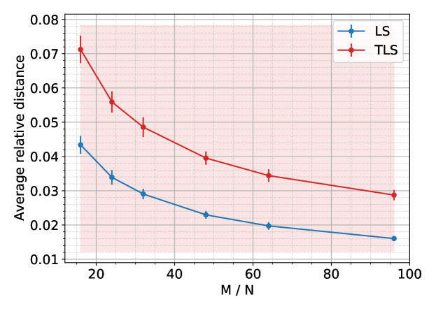
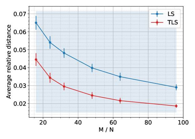
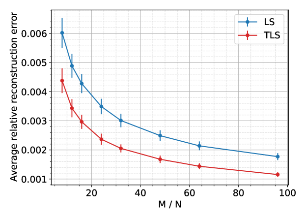
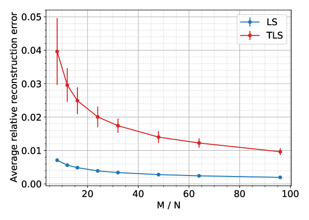
We plot the relative reconstruction errors as the oversampling ratio MN𝑀𝑁\frac{M}{N} is varied with N=100𝑁100N=100. Regularization parameters λysubscript𝜆𝑦\lambda_{y} and λasubscript𝜆𝑎\lambda_{a} are set to one. For each value of MN𝑀𝑁\frac{M}{N} we do 100 trials and each trial uses new sensing vectors, ground truth signals and errors. The standard deviation of the trials is indicated by error bars in the upcoming plots. The sensing vectors and ground truth signal are iid standard real Gaussian. Furthermore, the measurement and sensing vector errors are iid zero-mean real Gaussian with variance such that the sensing vector SNR is 40 dB. In Fig. 2a the measurement SNR is 65 dB and TLS has lower reconstruction error than LS. When the measurement SNR decreases to 40 dB in Fig. 2b, LS outperforms TLS. Although these experiments use the first-order error, they are consistent with our intuition. The relative performance of TLS is better when most of the error is due to sensing vector error. We also see that the performance of both methods improves as the number of measurements increases. Lastly, from Fig. 2b, TLS may improve relatively faster than LS as the number of measurements increase.
Refer to caption
(a) Measurement SNR is 65 dB.
Refer to caption
(b) Measurement SNR is 40 dB.
Figure 2: Relative reconstruction errors, (45) and (46) for different values of MN𝑀𝑁\frac{M}{N} when sensing vector SNR is 40 dB and measurement SNR is varied. All errors are Gaussian.
Refer to caption
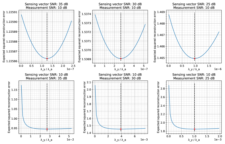
Figure 3: The TLS expected squared reconstruction error (47) is plotted for different ratios, λyλasubscript𝜆𝑦subscript𝜆𝑎\frac{\lambda_{y}}{\lambda_{a}}, to verify the optimal maximum likelihood parameters. Each subplot shows a different combination of sensing vector and measurement SNR. The minima are marked in red and the theoretically optimal ratio is indicated by the dashed black lines.

Verification of optimal ML parameters

The expression for TLS (47) in Proposition 4 enables us to verify the optimal maximum likelihood parameters for λysubscript𝜆𝑦\lambda_{y} and λasubscript𝜆𝑎\lambda_{a} from Proposition 2. Although Proposition 2 is stated for the complex-valued phase retrieval problem, the same procedure shows that the optimal parameters are the same for real-valued phase retrieval we considered here. The theoretically optimal parameter ratio is λyλa=σ𝜹2ση2subscript𝜆𝑦subscript𝜆𝑎subscriptsuperscript𝜎2𝜹subscriptsuperscript𝜎2𝜂\dfrac{\lambda_{y}}{\lambda_{a}}=\dfrac{\sigma^{2}_{\bm{{\delta}}}}{\sigma^{2}_{\eta}}.

To verify numerically whether this agrees with Proposition 4, we vary λyλasubscript𝜆𝑦subscript𝜆𝑎\frac{\lambda_{y}}{\lambda_{a}} (which is contained in 𝑫𝑫\bm{{D}}) around the optimal ratio and plot the TLS expression (47). We do this multiple times and in each run use a different iid standard real Gaussian ground truth signal and a different set of iid standard real Gaussian sensing vectors. As in Proposition 4, the errors in each run are iid zero-mean Gaussian and their variances are set to obtain different SNRs. Fig. 3 shows the different runs with the minima marked in red and the theoretically optimal ratio indicated by the dashed black lines. We can see that all the minima are at the optimal ratio which verifies Proposition 2. In the top row, most of the error is due to measurement error and the optimal ratio is low. This further highlights that TLS sensing vector corrections are less important when most of the error is due to measurement error.

We further note that the consistency between Propositions 2 and 4 demonstrates that the first-order expressions can be used to explain the performance of our TLS framework. Section IV shows that the real reconstruction errors follow the same trends as the numerical simulations in this section.

IV TLS phase retrieval simulations

We compare the performance of TLS phase retrieval against LS phase retrieval through simulations.111Code available at https://github.com/swing-research/tls_phase. To obtain a LS solution we use the Wirtinger flow method [3].

In this section we set the regularization parameters of (TLS-PR2) to λa=1Nsubscript𝜆𝑎1𝑁\lambda_{a}=\frac{1}{N} and λy=1𝒙(0)24subscript𝜆𝑦1superscriptsubscriptdelimited-∥∥superscript𝒙024\lambda_{y}=\frac{1}{\left\lVert\bm{{x}}^{(0)}\right\rVert_{2}^{4}} in all experiments with 𝒙(0)superscript𝒙0\bm{{x}}^{(0)} being an initial guess for 𝒙#superscript𝒙#\bm{{x}}^{\#}. These regularization parameters are tuned later in Section V. We fix the ground truth signal to be iid complex Gaussian with N=100𝑁100N=100. Furthermore, the TLS and LS iterations are stopped when their objective function values change by less than 106superscript10610^{-6} between successive iterates. The ground truth signal, TLS solution and LS solution are denoted as 𝒙#superscript𝒙#\bm{{x}}^{\#}, 𝒙TLSsubscriptsuperscript𝒙TLS\bm{{x}}^{\dagger}_{\mathrm{TLS}} and 𝒙LSsubscriptsuperscript𝒙LS\bm{{x}}^{\dagger}_{\mathrm{LS}}. In all experiments we generate M𝑀M quadratic measurements using M𝑀M clean sensing vectors. The TLS and LS methods must then recover the signal 𝒙#superscript𝒙#\bm{{x}}^{\#} from erroneous measurements and sensing vectors. We use SNR, as defined in Section III, to quantify measurement and sensing vector error. Also as in Section III, the plots in this section indicate the standard deviation of the trials using error bars.

IV-A Measurement models

In our experiments we will consider the complex-valued Gaussian and coded diffraction pattern measurement models. However, Algorithm 1 is not restricted to these measurement models. Recently in optical computing applications, random Gaussian scattering media have been used to do rapid high-dimensional randomized linear algebra, kernel classification and dimensionality reduction using laser light [36, 37]. The coded diffraction pattern model modulates the signal with different patterns before taking the Fourier transform. It is inspired by the fact that in coherent x-ray imaging the field at the detector is the Fourier transform of the signal [9].

When using the Gaussian measurement model, the n𝑛nth entry of sensing vector m𝑚m, amnsubscript𝑎𝑚𝑛a_{mn}, is distributed by the complex normal distribution for the complex-valued problem, amn𝒩(0,1)+j𝒩(0,1)similar-tosubscript𝑎𝑚𝑛𝒩01𝑗𝒩01a_{mn}\sim\mathcal{N}(0,1)+j\mathcal{N}(0,1). For the real-valued problem it is the standard normal distribution, amn𝒩(0,1)similar-tosubscript𝑎𝑚𝑛𝒩01a_{mn}\sim\mathcal{N}(0,1). The Gaussian measurement model sensing vector entries are independent of each other and the sensing vectors are also independent of each other. A description of the coded diffraction pattern measurement model is in Appendix G.

In this section of the main paper, the complex Gaussian measurement model is used. In Appendix G-A these experiments are repeated for the coded diffraction pattern measurement model and the same behavior is seen.

IV-B Algorithm initialization

In our experiments we opt to do the initialization of the signal being recovered (line 3 of Algorithm 1) via a spectral initialization. This method comprising a spectral initialization followed by gradient descent updates has been proven to lead to globally optimal solutions for the LS phase retrieval problem (LS-PR) in an error-free setting under the Gaussian and coded diffraction pattern models [12, 3].

The spectral initialization is the leading eigenvector of the matrix mym𝒂m𝒂mN×Nsubscript𝑚subscript𝑦𝑚subscript𝒂𝑚superscriptsubscript𝒂𝑚superscript𝑁𝑁\sum_{m}y_{m}\bm{{a}}_{m}\bm{{a}}_{m}^{*}\in\mathbb{C}^{N\times N} which we efficiently compute using 50 power method iterations. This eigenvector is scaled appropriately by estimating the norm of the signal of interest as (12Mmym)1/2superscript12𝑀subscript𝑚subscript𝑦𝑚12\left(\frac{1}{2M}\sum_{m}y_{m}\right)^{1/2}.

IV-C Signal recovery

To evaluate performance we compute the distance between the ground truth signal and the recovered signal. As the value of the objective function (TLS-PR1) is the same for 𝒙𝒙\bm{{x}} and phase shifted ejφ𝒙superscripte𝑗𝜑𝒙\mathrm{e}^{j\varphi}\bm{{x}}, we cannot distinguish between 𝒙𝒙\bm{{x}} and its phase-shifted variant. We therefore use a standard definition of distance that is invariant to phase shifts which is detailed in Definition 1.

Definition 1.

Denote the ground truth as 𝐱#Nsuperscript𝐱#superscript𝑁\bm{{x}}^{\#}\in\mathbb{C}^{N} and let 𝐱Nsuperscript𝐱superscript𝑁\bm{{x}}^{\dagger}\in\mathbb{C}^{N} be a solution to the phase retrieval problem. The distance between 𝐱#superscript𝐱#\bm{{x}}^{\#} and 𝐱superscript𝐱\bm{{x}}^{\dagger}, dist(𝐱#,𝐱)distsuperscript𝐱#superscript𝐱\mathrm{dist}(\bm{{x}}^{\#},\bm{{x}}^{\dagger}), is defined as dist(𝐱#,𝐱)=minφ[0,2π)𝐱#ejφ𝐱2\mathrm{dist}(\bm{{x}}^{\#},\bm{{x}}^{\dagger})=\min_{\varphi\in[0,2\pi)}\left\lVert\bm{{x}}^{\#}-\mathrm{e}^{j\varphi}\bm{{x}}^{\dagger}\right\rVert_{2}. Furthermore, the relative distance is defined as rel.dist(𝐱#,𝐱)=dist(𝐱#,𝐱)𝐱#2formulae-sequencereldistsuperscript𝐱#superscript𝐱distsuperscript𝐱#superscript𝐱subscriptdelimited-∥∥superscript𝐱#2\mathrm{rel.dist}(\bm{{x}}^{\#},\bm{{x}}^{\dagger})=\frac{\mathrm{dist}(\bm{{x}}^{\#},\bm{{x}}^{\dagger})}{\left\lVert\bm{{x}}^{\#}\right\rVert_{2}} and the reconstruction SNR in dB is defined as 20log10(rel.dist(𝐱#,𝐱))-20\log_{10}(\mathrm{rel.dist}(\bm{{x}}^{\#},\bm{{x}}^{\dagger})).

Combinations of sensing vector and measurement error

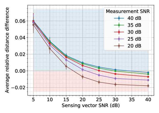
To understand how performance changes with different amounts of sensing vector and measurement error, we add different amounts of random iid complex Gaussian error to sensing vectors and random iid real Gaussian error to measurements. For each combination of sensing vector error and measurement error we perform 100 phase retrieval trials. In each trial we generate a new ground truth signal and M𝑀M new sensing vectors to produce M𝑀M new error-free measurements. In each trial we then add new random error perturbations to the sensing vectors and measurements. We evaluate performance by subtracting the relative distance of the TLS solution from that of the LS solution, (rel.dist(𝒙#,𝒙LS)rel.dist(𝒙#,𝒙TLS))formulae-sequencereldistsuperscript𝒙#subscriptsuperscript𝒙LSreldistsuperscript𝒙#subscriptsuperscript𝒙TLS(\mathrm{rel.dist}(\bm{{x}}^{\#},\bm{{x}}^{\dagger}_{\mathrm{LS}})-\mathrm{rel.dist}(\bm{{x}}^{\#},\bm{{x}}^{\dagger}_{\mathrm{TLS}})), and average across all 100 trials. If this average is positive, TLS has outperformed LS.

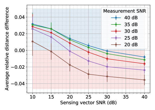
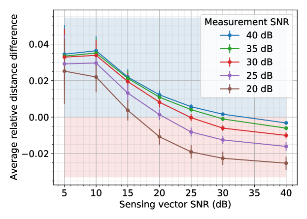
We use a step size of μ=0.5λa𝜇0.5subscript𝜆𝑎\mu=\frac{0.5}{\lambda_{a}} for TLS and μ=0.02𝜇0.02\mu=0.02 for LS to perform the gradient update for 𝒙𝒙\bm{{x}} in (7). The TLS step size is inversely proportional to λasubscript𝜆𝑎\lambda_{a} because the relative importance of the data consistency term is inversely proportional to the sensing vector consistency term in (TLS-PR2). Fig. 4 shows the performance for MN{8,16,32}𝑀𝑁81632\frac{M}{N}\in\{8,16,32\}. Note that the minimum sensing vector SNR is 10 dB when MN=8𝑀𝑁8\frac{M}{N}=8 and 5 dB in the other cases. For a fixed sensing vector SNR, the performance of TLS decreases when the measurement SNR decreases. This is expected because more of the error is in the measurements which LS is designed for. In general TLS is better when the sensing vector SNR decreases for a fixed measurement SNR because TLS phase retrieval accounts for sensing vector error. However, this trend starts to break for very low sensing vector SNR as shown at 5 dB when MN=16𝑀𝑁16\frac{M}{N}=16. Increasing the number of measurements overcomes this issue and in general improves TLS performance as was indicated by the first-order reconstruction errors with Gaussian error in Figs. 2a and 2b.
Refer to caption
(a) MN=8𝑀𝑁8\frac{M}{N}=8
Refer to caption
(b) MN=16𝑀𝑁16\frac{M}{N}=16
Refer to caption
(c) MN=32𝑀𝑁32\frac{M}{N}=32
Figure 4: Average difference in relative distance of TLS and LS solutions, rel.dist(𝒙#,𝒙LS)rel.dist(𝒙#,𝒙TLS)formulae-sequencereldistsuperscript𝒙#subscriptsuperscript𝒙LSreldistsuperscript𝒙#subscriptsuperscript𝒙TLS\mathrm{rel.dist}(\bm{{x}}^{\#},\bm{{x}}^{\dagger}_{\mathrm{LS}})-\mathrm{rel.dist}(\bm{{x}}^{\#},\bm{{x}}^{\dagger}_{\mathrm{TLS}}), for the Gaussian measurement model for different measurement and sensing vector SNR combinations when MN{8,16,32}𝑀𝑁81632\frac{M}{N}\in\{8,16,32\}.

Impact of varying the number of measurements

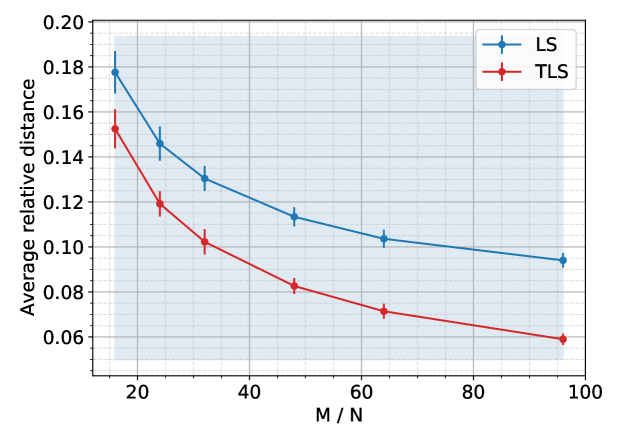
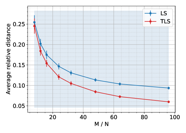
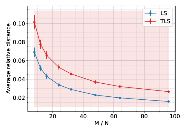
To clearly see the impact of varying the number of measurements we fix the measurement SNR to 20 dB and sensing vector SNR to 10 dB and plot the reconstruction relative distance for TLS and LS in Fig. 5a. We do 100 trials for each value of MN𝑀𝑁\frac{M}{N}. The performance improvement of TLS over LS increases as the number of measurements are increased. In Fig. 5b we increase the sensing vector SNR to 30 dB. When the balance of the Gaussian error shifts more towards the measurements, LS performs better. This is identical to what was seen with the first-order reconstruction errors in Figs. 2a and 2b.
Refer to caption
(a) Sensing vector SNR is 10 dB.
Refer to caption
(b) Sensing vector SNR is 30 dB.
Figure 5: Relative distance of reconstructions using TLS and LS for the Gaussian measurement model for different MN𝑀𝑁\frac{M}{N} when measurement SNR is 20 dB and measurement SNR is varied. All errors are Gaussian.

Accuracy of first-order reconstruction errors

Appendix E contains the description of an experiment where we verify the accuracy of the reconstruction error expressions in Proposition 3 against the real errors. As expected, it shows that the first-order expressions in Proposition 3 increase in accuracy as the sensing vector and measurement error decreases—this corresponds to the norm of 𝜸𝜸\bm{{\gamma}} in (27) decreasing, but that these expressions may only serve as a rough rule of thumb when errors are large.

Sensing vectors and measurements error model

The simulations in this section use iid random Gaussian errors. In Appendix F we design errors that require access to the ground truth signal norm and to the error-free measurements. We show that the improvement of TLS over LS can be larger in this artificial scenario.

IV-D Corrected sensing vector verification

To characterize the sensing vector corrections performed by our algorithm, we define a metric sensitive to the relative correction error of the sensing vectors. The metric only considers corrections in the direction of the recovered signal because our algorithm only corrects the component of the sensing vectors in the direction of this signal due to the optimization geometry (Section II-A).

Definition 2.

Denote the complex-valued ground truth signal and sensing vectors as 𝐱#superscript𝐱#\bm{{x}}^{\#} and 𝐚#:={𝐚m#}m=1Massignsuperscript𝐚#superscriptsubscriptsubscriptsuperscript𝐚#𝑚𝑚1𝑀\bm{{a}}^{\#}:=\{\bm{{a}}^{\#}_{m}\}_{m=1}^{M}. Let their counterparts obtained by solving the TLS phase retrieval problem be 𝐱superscript𝐱\bm{{x}}^{\dagger} and 𝐚:={𝐚m}m=1Massignsuperscript𝐚superscriptsubscriptsubscriptsuperscript𝐚𝑚𝑚1𝑀\bm{{a}}^{\dagger}:=\{\bm{{a}}^{\dagger}_{m}\}_{m=1}^{M}. Further let φ=argminφ[0,2π)𝐱#ejφ𝐱2\varphi=\operatorname*{arg\,min}_{\varphi\in[0,2\pi)}\left\lVert\bm{{x}}^{\#}-\mathrm{e}^{j\varphi}\bm{{x}}^{\dagger}\right\rVert_{2}. Then, denoting 𝗒(𝐚,𝐱)=[𝐚1,𝐱,,𝐚M,𝐱]𝗒𝐚𝐱subscript𝐚1𝐱subscript𝐚𝑀𝐱\mathsf{y}(\bm{{a}},\bm{{x}})=\left[\left\langle\bm{{a}}_{1},\bm{{x}}\right\rangle,\ldots,\left\langle\bm{{a}}_{M},\bm{{x}}\right\rangle\right], the relative sensing vector correction error between 𝐚#superscript𝐚#\bm{{a}}^{\#} and 𝐚superscript𝐚\bm{{a}}^{\dagger} is defined as rel.corr({𝐚#,𝐱#},{𝐚,𝐱})=𝗒(𝐚#,𝐱#)𝗒(𝐚,ejφ𝐱)2𝗒(𝐚#,𝐱#)2formulae-sequencerelcorrsuperscript𝐚#superscript𝐱#superscript𝐚superscript𝐱subscriptdelimited-∥∥𝗒superscript𝐚#superscript𝐱#𝗒superscript𝐚superscripte𝑗𝜑superscript𝐱2subscriptdelimited-∥∥𝗒superscript𝐚#superscript𝐱#2\mathrm{rel.corr}(\{\bm{{a}}^{\#},\,\bm{{x}}^{\#}\},\{\bm{{a}}^{\dagger},\,\bm{{x}}^{\dagger}\})=\dfrac{\left\lVert\mathsf{y}(\bm{{a}}^{\#},\,\bm{{x}}^{\#})-\mathsf{y}(\bm{{a}}^{\dagger},\,\mathrm{e}^{j\varphi}\bm{{x}}^{\dagger})\right\rVert_{2}}{\left\lVert\mathsf{y}(\bm{{a}}^{\#},\,\bm{{x}}^{\#})\right\rVert_{2}}.

To evaluate performance, we denote the ground truth and TLS corrected sensing vectors as {𝒂~m}m=1Msuperscriptsubscriptsubscript~𝒂𝑚𝑚1𝑀\{\widetilde{\bm{{a}}}_{m}\}_{m=1}^{M} and {𝒂^m}m=1Msuperscriptsubscriptsubscriptsuperscript^𝒂𝑚𝑚1𝑀\{\widehat{\bm{{a}}}^{\dagger}_{m}\}_{m=1}^{M}. For the sensing vectors in the previous experiments of Fig. 4 we compute rel.corr({𝒂~,𝒙#},{𝒂^,𝒙TLS})formulae-sequencerelcorr~𝒂superscript𝒙#superscript^𝒂subscriptsuperscript𝒙TLS\mathrm{rel.corr}(\{\widetilde{\bm{{a}}},\,\bm{{x}}^{\#}\},\{\widehat{\bm{{a}}}^{\dagger},\,\bm{{x}}^{\dagger}_{\mathrm{TLS}}\}) and average across the 100 trials. Fig. 6 shows the relative correction error when MN{16,32}𝑀𝑁1632\frac{M}{N}\in\{16,32\}. We see that as the sensing vector SNR increases, the relative correction error decreases. Furthermore, as the measurement SNR decreases, the relative correction error increases. These relative correction error increases are more pronounced when the sensing vector SNR is high, a setting where sensing vector correction is needed less. This observation is consistent with Fig. 4—when sensing vector SNR is high, the TLS sensing vector corrections hinder TLS performance and LS outperforms TLS.
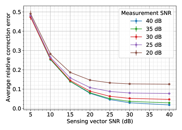
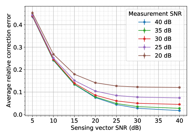
Refer to caption
(a) MN=16𝑀𝑁16\frac{M}{N}=16
Refer to caption
(b) MN=32𝑀𝑁32\frac{M}{N}=32
Figure 6: Average relative sensing vector correction error when using TLS, rel.corr({𝒂~,𝒙#},{𝒂^,ejφ𝒙TLS)\mathrm{rel.corr}(\{\widetilde{\bm{{a}}},\,\bm{{x}}^{\#}\},\{\widehat{\bm{{a}}}^{\dagger},\,\mathrm{e}^{j\varphi}\bm{{x}}^{\dagger}_{\mathrm{TLS}}), for the Gaussian measurement model for different measurement and sensing vector SNR combinations when MN{16,32}𝑀𝑁1632\frac{M}{N}\in\{16,32\}.

Next we investigate how the number of measurements impacts the relative correction error. We do this with the sensing vectors from the previous experiments in Figs. 5a and 5b. Fig. 7 shows the averages over the 100 trials. Here the measurement SNR was fixed to 20 dB and the sensing vector SNR was 10 dB or 30 dB. Consistent with what was seen previously, the performance of TLS improves with increasing number of measurements. Additionally, increasing the number of measurements provides greater gains when the sensing vector SNR is lower.
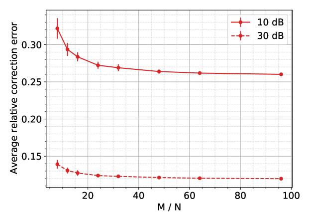
Refer to caption
Figure 7: Relative sensing vector correction error when using TLS for the Gaussian measurement model for different MN𝑀𝑁\frac{M}{N} when measurement SNR is 20 dB. The sensing vector SNR is 10 dB or 30 dB.

V Experiments on real optical hardware

In this section we show that TLS phase retrieval outperforms LS phase retrieval when using real optical hardware. We use an Optical Processing Unit (OPU) which enables rapid random high-dimensional matrix-vector multiplication.222Visit https://www.lighton.ai/lighton-cloud/ for a publicly available cloud OPU with a scikit-learn interface. A known signal 𝒙#Nsuperscript𝒙#superscript𝑁\bm{{x}}^{\#}\in\mathbb{R}^{N} is encoded onto coherent laser light using a digital micro-mirror device (DMD) which is then shined through a Gaussian multiple scattering medium as shown in Fig. 8. We denote the transmission matrix of the Gaussian medium as 𝑨M×N𝑨superscript𝑀𝑁\bm{{A}}\in\mathbb{C}^{M\times N}. The M𝑀M rows of the transmission matrix are sensing vectors, 𝒂mNsubscript𝒂𝑚superscript𝑁\bm{{a}}_{m}\in\mathbb{C}^{N} for 1mM1𝑚𝑀1\leq m\leq M. The intensity of the scattered light in the sensor plane, ym|𝒂m,𝒙#|2subscript𝑦𝑚superscriptsubscript𝒂𝑚superscript𝒙#2y_{m}\approx{\left|\left\langle\bm{{a}}_{m},\bm{{x}}^{\#}\right\rangle\right|}^{2} for all m𝑚m, is then measured using a camera. We do phase retrieval using the optical measurements to reconstruct the input, 𝒙#superscript𝒙#\bm{{x}}^{\#}. The input signals are limited to real-valued binary images due to the DMD.

Refer to caption
DMD encoding
of 𝒙#Nsuperscript𝒙#superscript𝑁\bm{{x}}^{\#}\in\mathbb{R}^{N}

|𝒂m,𝒙#|2ymsuperscriptsubscript𝒂𝑚superscript𝒙#2subscript𝑦𝑚{\left|\left\langle\bm{{a}}_{m},\bm{{x}}^{\#}\right\rangle\right|}^{2}\approx y_{m}

Random
scattering
medium
Camera
taking 8-bit
measurements
Refer to caption

𝒂miid𝒩(0,𝑰)+j𝒩(0,𝑰)subscript𝒂𝑚iidsimilar-to𝒩0𝑰𝑗𝒩0𝑰\bm{{a}}_{m}\overset{\text{iid}}{\sim}\mathcal{N}(0,\bm{{I}})+j\mathcal{N}(0,\bm{{I}})

Laser
light
source
Figure 8: The optical processing unit (OPU). A coherent laser beam spatially encodes a signal, 𝒙𝒙\bm{{x}}, via a digital micro-mirror device (DMD) which is then shined through a random medium. A camera measures the squared magnitude of the scattered light.

The OPU measurements and sensing vectors both contain errors. Errors in the optical measurements are caused by 8-bit quantized camera measurements and Poisson noise which scales with the square root of the mean intensity of the scattered light. Additionally, there are measurement errors due to thermal effects and other system properties that result in a noise floor. Thus the lowest intensity that can be measured is not zero, even if an all-zero signal, 𝒙#=𝟎superscript𝒙#0\bm{{x}}^{\#}=\bm{{0}}, is encoded on the laser light and shined through the scattering medium. The sensing vectors are erroneous because the entries of 𝑨𝑨\bm{{A}} are unknown and must be calibrated from erroneous optical measurements [2]. There may also be other sources of experimental error. Unlike in the computer simulations of Section IV, when using the OPU, we do not know the exact error model and we also do not know the levels of the errors in the measurements and sensing vectors.

In the experiments, the TLS and LS step sizes are tuned to 0.4λa0.4subscript𝜆𝑎\frac{0.4}{\lambda_{a}} and 0.005. The initialization method and termination criteria are the same as in Section IV. Additionally, we use the fact that the images being reconstructed are real-valued and binary to regularize both the TLS and LS methods. After the initialization (Algorithm 1, Step 3 for TLS) and each 𝒙𝒙\bm{{x}} update step (Algorithm 1, Step 19 for TLS) we take the elementwise absolute value of the signal to set the phase of all elements to zero. We then normalize the entries of 𝒙TLSsubscriptsuperscript𝒙TLS\bm{{x}}^{\dagger}_{\mathrm{TLS}} and 𝒙LSsubscriptsuperscript𝒙LS\bm{{x}}^{\dagger}_{\mathrm{LS}} with absolute value larger than one to one.

Appendix H contains details of the sensing vector calibration method used and further OPU experimental details.

Random ground truth signals

Our ground truth signals are real-valued random binary images of size N=16×16=256𝑁1616256N=16\times 16=256. We vary the oversampling ratio, MN𝑀𝑁\frac{M}{N}, and perform 100 trials for each ratio. In each trial a new ground truth image and set of calibrated sensing vectors is used. On a held out set of ten images and with MN=8𝑀𝑁8\frac{M}{N}=8 we tune λa=40subscript𝜆𝑎40\lambda_{a}=40 and λy=𝒙(0)24subscript𝜆𝑦superscriptsubscriptdelimited-∥∥superscript𝒙024\lambda_{y}=\left\lVert\bm{{x}}^{(0)}\right\rVert_{2}^{-4} in (TLS-PR2) where 𝒙(0)superscript𝒙0\bm{{x}}^{(0)} is the initialization. Fig. 9 shows that the SNR of the reconstructed images using TLS is higher than when using LS for all numbers of measurements. Additionally, in Fig. 10 we plot the standard deviation of the results in Fig. 9 and show that the TLS method has lower variability.
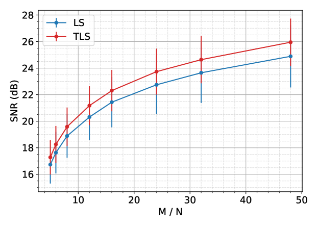
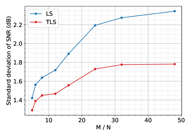
Refer to caption
Figure 9: SNR of reconstructed random binary images when using TLS and LS for phase retrieval on the OPU. Values of MN𝑀𝑁\frac{M}{N} between five and 48 are used.
Refer to caption
Figure 10: Standard deviation of the SNR in Fig. 9 when random binary images are reconstructed on the OPU.

Real image ground truth signals

We reconstruct binary images of size N=32×32=1024𝑁32321024N=32\times 32=1024 for MN{5,8,12}𝑀𝑁5812\frac{M}{N}\in\{5,8,12\}. On a held out set of five images and with MN=5𝑀𝑁5\frac{M}{N}=5 we tune λa=20subscript𝜆𝑎20\lambda_{a}=20 and again λy=𝒙(0)24subscript𝜆𝑦superscriptsubscriptdelimited-∥∥superscript𝒙024\lambda_{y}=\left\lVert\bm{{x}}^{(0)}\right\rVert_{2}^{-4} in (TLS-PR2) where 𝒙(0)superscript𝒙0\bm{{x}}^{(0)} is the initialization. Fig. 11 shows the original images, their reconstructions and their reconstruction SNR. For a given oversampling ratio, the TLS approach reports better SNR values and reconstructs images of better visual quality as compared to the LS approach.

Refer to caption
Figure 11: Reconstructions of 32×32323232\times 32 images and reconstruction SNR when using TLS and LS on the OPU. The oversampling ratio is varied.

VI Conclusion

We have developed a TLS framework for solving the phase retrieval problem that accounts for both sensing vector error and measurement error. One of the keys to solving the TLS problem via gradient descent was studying the geometry of the TLS optimization problem to realize that the sensing vectors can be efficiently updated by solving a scalar variable optimization problem instead of a vector variable optimization problem. By deriving the Taylor series expansions for the TLS and LS solutions we have also obtained approximate expressions for their reconstruction error. These expressions enabled us to anticipate the accuracy of the TLS solution relative to the LS solution and understand when which approach will lead to a better solution. We verify the TLS method through a range of computer simulations. Furthermore, in experiments with real optical hardware, TLS outperforms LS.

Presently we correct the sensing vectors based on the one signal that we wish to recover. An interesting future line of work lies in multi-signal TLS for sensing vector denoising so that subsequent signals can be recovered without requiring sensing vector corrections if their measurements use the same set of sensing vectors. There are multiple areas where this is required. An upcoming application is in optical neural network backpropagation where unknown random sensing vectors are the rows of weight matrices of fully-connected layers. Denoised and more accurate rows will enable better machine learning performance.

There exist other applications of phase retrieval with uncertain sensing vectors. Ptychography, which can be modeled analogously to (1), is a prime example [38]. Ptychography has recently been addressed by least squares, comprising spectral initialization followed by gradient descent [39]. It would be interesting to see whether our TLS phase retrieval algorithm brings about improvements. Other ptychography methods use alternating updates to recover the object and the sensing vectors [40]. Our geometric intuition may help reduce the number of unknowns in sensing vector updates and thus improve the overall computational efficiency of these algorithms.

Appendix A Roots of cubic equations

Consider finding the roots of the following cubic equation

ax3+bx2+cx+d=0.𝑎superscript𝑥3𝑏superscript𝑥2𝑐𝑥𝑑0\displaystyle ax^{3}+bx^{2}+cx+d=0. (49)

Denote

ψ0subscript𝜓0\displaystyle\psi_{0} =b23acabsentsuperscript𝑏23𝑎𝑐\displaystyle=b^{2}-3ac (50)
ψ1subscript𝜓1\displaystyle\psi_{1} =2b39abc+27a2dabsent2superscript𝑏39𝑎𝑏𝑐27superscript𝑎2𝑑\displaystyle=2b^{3}-9abc+27a^{2}d (51)
ψ3subscript𝜓3\displaystyle\psi_{3} =ψ1+ψ124ψ0323.absent3subscript𝜓1superscriptsubscript𝜓124superscriptsubscript𝜓032\displaystyle=\sqrt[3]{\frac{\psi_{1}+\sqrt{\psi_{1}^{2}-4\psi_{0}^{3}}}{2}}. (52)

Then for k{0,1,2}𝑘012k\in\{0,1,2\} the three roots, xksubscript𝑥𝑘x_{k}, are

xk=13a(b+θkψ3+ψ0θkψ3)subscript𝑥𝑘13𝑎𝑏superscript𝜃𝑘subscript𝜓3subscript𝜓0superscript𝜃𝑘subscript𝜓3\displaystyle x_{k}=-\frac{1}{3a}\left(b+\theta^{k}\psi_{3}+\frac{\psi_{0}}{\theta^{k}\psi_{3}}\right) (53)

where θ𝜃\theta is the cube root of unity, θ=1+32𝜃132\theta=\frac{-1+\sqrt{-3}}{2}.

Note that the cubic equations in this paper are with b=0𝑏0b=0 which simplifies the above expressions.

Appendix B Proof of Proposition 2

The ML estimator estimates both 𝒙~~𝒙\widetilde{\bm{{x}}} and {𝒂~m}m=1Msuperscriptsubscriptsubscript~𝒂𝑚𝑚1𝑀\{\widetilde{\bm{{a}}}_{m}\}_{m=1}^{M} from the data {ym}m=1Msuperscriptsubscriptsubscript𝑦𝑚𝑚1𝑀\{y_{m}\}_{m=1}^{M} and {𝒂m}m=1Msuperscriptsubscriptsubscript𝒂𝑚𝑚1𝑀\{\bm{{a}}_{m}\}_{m=1}^{M} by minimizing the negative conditional log-likelihood

argmin𝒙,𝒆1,,𝒆Mln(m=1MPr{ym,𝒂m|𝒙~=𝒙,𝒂~m=𝒂m+𝒆m})subscriptargmin𝒙subscript𝒆1subscript𝒆𝑀superscriptsubscriptproduct𝑚1𝑀Prconditional-setsubscript𝑦𝑚subscript𝒂𝑚formulae-sequence~𝒙𝒙subscript~𝒂𝑚subscript𝒂𝑚subscript𝒆𝑚\displaystyle\operatorname*{arg\,min}_{\bm{{x}},\bm{{e}}_{1},\ldots,\bm{{e}}_{M}}-\ln\left(\prod_{m=1}^{M}\mathrm{Pr}\{y_{m},\bm{{a}}_{m}|\widetilde{\bm{{x}}}=\bm{{x}},\widetilde{\bm{{a}}}_{m}=\bm{{a}}_{m}+\bm{{e}}_{m}\}\right)

With 𝒙~~𝒙\widetilde{\bm{{x}}} and {𝒂~m}m=1Msuperscriptsubscriptsubscript~𝒂𝑚𝑚1𝑀\{\widetilde{\bm{{a}}}_{m}\}_{m=1}^{M} given, the only randomness in each ymsubscript𝑦𝑚y_{m} and 𝒂msubscript𝒂𝑚\bm{{a}}_{m} are due to ηmsubscript𝜂𝑚\eta_{m} and 𝜹msubscript𝜹𝑚\bm{{\delta}}_{m}. Furthermore as {ηm}m=1Msuperscriptsubscriptsubscript𝜂𝑚𝑚1𝑀\{\eta_{m}\}_{m=1}^{M} and {𝜹m}m=1Msuperscriptsubscriptsubscript𝜹𝑚𝑚1𝑀\{\bm{{\delta}}_{m}\}_{m=1}^{M} are independent, the negative conditional log-likelihood is,

m=1Mln(Pr{ηm=\displaystyle\sum_{m=1}^{M}-\ln(\mathrm{Pr}\{\eta_{m}= |𝒂m+𝒆m,𝒙|2ym})\displaystyle{\left|\left\langle\bm{{a}}_{m}+\bm{{e}}_{m},\bm{{x}}\right\rangle\right|}^{2}-y_{m}\})
ln(Pr{𝜹m=𝒆m}).Prsubscript𝜹𝑚subscript𝒆𝑚\displaystyle-\ln(\mathrm{Pr}\{\bm{{\delta}}_{m}=\bm{{e}}_{m}\}). (54)

Using the assumptions on the error distributions,

ln(Pr{ηm=\displaystyle\ln(\mathrm{Pr}\{\eta_{m}= |𝒂m+𝒆m,𝒙|2ym})\displaystyle{\left|\left\langle\bm{{a}}_{m}+\bm{{e}}_{m},\bm{{x}}\right\rangle\right|}^{2}-y_{m}\})
=\displaystyle= Kη12ση2(ym|𝒂m+𝒆m,𝒙|2)2subscript𝐾𝜂12superscriptsubscript𝜎𝜂2superscriptsubscript𝑦𝑚superscriptsubscript𝒂𝑚subscript𝒆𝑚𝒙22\displaystyle K_{\eta}-\frac{1}{2\sigma_{\eta}^{2}}\left(y_{m}-{\left|\left\langle\bm{{a}}_{m}+\bm{{e}}_{m},\bm{{x}}\right\rangle\right|}^{2}\right)^{2} (55)

and

ln(Pr{𝜹m=𝒆m})=K𝜹12σ𝜹2𝒆m22Prsubscript𝜹𝑚subscript𝒆𝑚subscript𝐾𝜹12subscriptsuperscript𝜎2𝜹superscriptsubscriptdelimited-∥∥subscript𝒆𝑚22\displaystyle\ln\left(\mathrm{Pr}\left\{\bm{{\delta}}_{m}=\bm{{e}}_{m}\right\}\right)=K_{\bm{{\delta}}}-\frac{1}{2\sigma^{2}_{\bm{{\delta}}}}\left\lVert\bm{{e}}_{m}\right\rVert_{2}^{2} (56)

where Kηsubscript𝐾𝜂K_{\eta} and K𝜹subscript𝐾𝜹K_{\bm{{\delta}}} are constants independent of 𝒙𝒙\bm{{x}} and {𝒆m}m=1Msuperscriptsubscriptsubscript𝒆𝑚𝑚1𝑀\{\bm{{e}}_{m}\}_{m=1}^{M}. Substituting these into (54) gives

argmin𝒙,𝒆1,,𝒆Mm=1M1σ𝜹2𝒆m22+1ση2(ym|𝒂m+𝒆m,𝒙|2)2.subscriptargmin𝒙subscript𝒆1subscript𝒆𝑀superscriptsubscript𝑚1𝑀1subscriptsuperscript𝜎2𝜹superscriptsubscriptdelimited-∥∥subscript𝒆𝑚221subscriptsuperscript𝜎2𝜂superscriptsubscript𝑦𝑚superscriptsubscript𝒂𝑚subscript𝒆𝑚𝒙22\displaystyle\operatorname*{arg\,min}_{\bm{{x}},\bm{{e}}_{1},\ldots,\bm{{e}}_{M}}\sum_{m=1}^{M}\frac{1}{\sigma^{2}_{\bm{{\delta}}}}\left\lVert\bm{{e}}_{m}\right\rVert_{2}^{2}+\frac{1}{\sigma^{2}_{\eta}}\left(y_{m}-{\left|\left\langle\bm{{a}}_{m}+\bm{{e}}_{m},\bm{{x}}\right\rangle\right|}^{2}\right)^{2}.

References

  • [1] T. Bendory, R. Beinert, and Y. C. Eldar, “Fourier phase retrieval: Uniqueness and algorithms,” in Compressed Sensing and its Applications.   Springer, 2017, pp. 55–91.
  • [2] S. Gupta, R. Gribonval, L. Daudet, and I. Dokmanić, “Fast optical system identification by numerical interferometry,” in ICASSP 2020-2020 IEEE International Conference on Acoustics, Speech and Signal Processing (ICASSP).   IEEE, 2020, pp. 1474–1478.
  • [3] E. J. Candes, X. Li, and M. Soltanolkotabi, “Phase retrieval via wirtinger flow: Theory and algorithms,” IEEE Transactions on Information Theory, vol. 61, no. 4, pp. 1985–2007, 2015.
  • [4] G. H. Golub and C. F. Van Loan, “An analysis of the total least squares problem,” SIAM journal on numerical analysis, vol. 17, no. 6, pp. 883–893, 1980.
  • [5] I. Markovsky and S. Van Huffel, “Overview of total least-squares methods,” Signal processing, vol. 87, no. 10, pp. 2283–2302, 2007.
  • [6] P. T. Boggs, R. H. Byrd, and R. B. Schnabel, “A stable and efficient algorithm for nonlinear orthogonal distance regression,” SIAM Journal on Scientific and Statistical Computing, vol. 8, no. 6, pp. 1052–1078, 1987.
  • [7] R. W. Gerchberg, “A practical algorithm for the determination of phase from image and diffraction plane pictures,” Optik, vol. 35, pp. 237–246, 1972.
  • [8] J. R. Fienup, “Reconstruction of an object from the modulus of its fourier transform,” Optics letters, vol. 3, no. 1, pp. 27–29, 1978.
  • [9] R. E. Blahut, Theory of remote image formation.   Cambridge University Press, 2004, ch. 8, p. 254–286.
  • [10] B. Rajaei, S. Gigan, F. Krzakala, and L. Daudet, “Robust phase retrieval with the swept approximate message passing (prsamp) algorithm,” Image Processing On Line, vol. 7, pp. 43–55, 2017.
  • [11] M. K. Sharma, C. A. Metzler, S. Nagesh, R. G. Baraniuk, O. Cossairt, and A. Veeraraghavan, “Inverse scattering via transmission matrices: Broadband illumination and fast phase retrieval algorithms,” IEEE Transactions on Computational Imaging, vol. 6, pp. 95–108, 2019.
  • [12] P. Netrapalli, P. Jain, and S. Sanghavi, “Phase retrieval using alternating minimization,” in Advances in Neural Information Processing Systems, 2013, pp. 2796–2804.
  • [13] G. Wang, G. B. Giannakis, and Y. C. Eldar, “Solving systems of random quadratic equations via truncated amplitude flow,” IEEE Transactions on Information Theory, vol. 64, no. 2, pp. 773–794, 2017.
  • [14] Y. Chen and E. Candes, “Solving random quadratic systems of equations is nearly as easy as solving linear systems,” in Advances in Neural Information Processing Systems, 2015, pp. 739–747.
  • [15] S. Huang, S. Gupta, and I. Dokmanić, “Solving complex quadratic systems with full-rank random matrices,” IEEE Transactions on Signal Processing, vol. 68, pp. 4782–4796, 2020.
  • [16] S. Huang and I. Dokmanić, “Reconstructing point sets from distance distributions,” arXiv preprint arXiv:1804.02465, 2018.
  • [17] T. T. Cai, X. Li, Z. Ma et al., “Optimal rates of convergence for noisy sparse phase retrieval via thresholded wirtinger flow,” The Annals of Statistics, vol. 44, no. 5, pp. 2221–2251, 2016.
  • [18] G. Wang, L. Zhang, G. B. Giannakis, M. Akçakaya, and J. Chen, “Sparse phase retrieval via truncated amplitude flow,” IEEE Transactions on Signal Processing, vol. 66, no. 2, pp. 479–491, 2017.
  • [19] M. A. Davenport and J. Romberg, “An overview of low-rank matrix recovery from incomplete observations,” IEEE Journal of Selected Topics in Signal Processing, vol. 10, no. 4, pp. 608–622, 2016.
  • [20] E. J. Candes, Y. C. Eldar, T. Strohmer, and V. Voroninski, “Phase retrieval via matrix completion,” SIAM review, vol. 57, no. 2, pp. 225–251, 2015.
  • [21] E. J. Candes, T. Strohmer, and V. Voroninski, “Phaselift: Exact and stable signal recovery from magnitude measurements via convex programming,” Communications on Pure and Applied Mathematics, vol. 66, no. 8, pp. 1241–1274, 2013.
  • [22] A. Yurtsever, M. Udell, J. Tropp, and V. Cevher, “Sketchy decisions: Convex low-rank matrix optimization with optimal storage,” in Artificial intelligence and statistics.   PMLR, 2017, pp. 1188–1196.
  • [23] T. Goldstein and C. Studer, “Phasemax: Convex phase retrieval via basis pursuit,” IEEE Transactions on Information Theory, vol. 64, no. 4, pp. 2675–2689, 2018.
  • [24] S. Van Huffel and J. Vandewalle, “On the accuracy of total least squares and least squares techniques in the presence of errors on all data,” Automatica, vol. 25, no. 5, pp. 765–769, 1989.
  • [25] I. Markovsky, J. C. Willems, S. Van Huffel, B. De Moor, and R. Pintelon, “Application of structured total least squares for system identification and model reduction,” IEEE Transactions on Automatic Control, vol. 50, no. 10, pp. 1490–1500, 2005.
  • [26] D. Malioutov and N. Slavov, “Convex total least squares,” in International Conference on Machine Learning, 2014, pp. 109–117.
  • [27] H. Zhu, G. Leus, and G. B. Giannakis, “Sparsity-cognizant total least-squares for perturbed compressive sampling,” IEEE Transactions on Signal Processing, vol. 59, no. 5, pp. 2002–2016, 2011.
  • [28] D. M. Sima, S. Van Huffel, and G. H. Golub, “Regularized total least squares based on quadratic eigenvalue problem solvers,” BIT Numerical Mathematics, vol. 44, no. 4, pp. 793–812, 2004.
  • [29] A. E. Yagle and A. E. Bell, “One-and two-dimensional minimum and nonminimum phase retrieval by solving linear systems of equations,” IEEE Transactions on Signal Processing, vol. 47, no. 11, pp. 2978–2989, 1999.
  • [30] H. Schwetlick and V. Tiller, “Numerical methods for estimating parameters in nonlinear models with errors in the variables,” Technometrics, vol. 27, no. 1, pp. 17–24, 1985.
  • [31] D. Powell and J. Macdonald, “A rapidly convergent iterative method for the solution of the generalised nonlinear least squares problem,” The Computer Journal, vol. 15, no. 2, pp. 148–155, 1972.
  • [32] A. Wiesel, Y. C. Eldar, and A. Beck, “Maximum likelihood estimation in linear models with a gaussian model matrix,” IEEE Signal Processing Letters, vol. 13, no. 5, pp. 292–295, 2006.
  • [33] S. Gould, B. Fernando, A. Cherian, P. Anderson, R. S. Cruz, and E. Guo, “On differentiating parameterized argmin and argmax problems with application to bi-level optimization,” arXiv preprint arXiv:1607.05447, 2016.
  • [34] R. Balan, P. Casazza, and D. Edidin, “On signal reconstruction without phase,” Applied and Computational Harmonic Analysis, vol. 20, no. 3, pp. 345–356, 2006.
  • [35] A. Conca, D. Edidin, M. Hering, and C. Vinzant, “An algebraic characterization of injectivity in phase retrieval,” Applied and Computational Harmonic Analysis, vol. 38, no. 2, pp. 346–356, 2015.
  • [36] S. Gupta, R. Gribonval, L. Daudet, and I. Dokmanić, “Don’t take it lightly: Phasing optical random projections with unknown operators,” in Advances in Neural Information Processing Systems, 2019, pp. 14 855–14 865.
  • [37] A. Saade, F. Caltagirone, I. Carron, L. Daudet, A. Drémeau, S. Gigan, and F. Krzakala, “Random projections through multiple optical scattering: Approximating kernels at the speed of light,” in 2016 IEEE International Conference on Acoustics, Speech and Signal Processing (ICASSP).   IEEE, 2016, pp. 6215–6219.
  • [38] F. Pfeiffer, “X-ray ptychography,” Nature Photonics, vol. 12, no. 1, pp. 9–17, 2018.
  • [39] L. Valzania, J. Dong, and S. Gigan, “Accelerating ptychographic reconstructions using spectral initializations,” Optics Letters, vol. 46, no. 6, pp. 1357–1360, 2021.
  • [40] A. Maiden, D. Johnson, and P. Li, “Further improvements to the ptychographical iterative engine,” Optica, vol. 4, no. 7, pp. 736–745, 2017.
  • [41] E. J. Candes, X. Li, and M. Soltanolkotabi, “Phase retrieval from coded diffraction patterns,” Applied and Computational Harmonic Analysis, vol. 39, no. 2, pp. 277–299, 2015.

Supplementary material

Appendix C Taylor series expansions

Lemma 1 states the Taylor series expansions around the no error point 𝒕~~𝒕\widetilde{\bm{{t}}} for the TLS and LS solutions. The notation defined in Section III is used.

Lemma 1.

The Taylor series expansions for the solution 𝐱TLSsuperscriptsubscript𝐱TLS\bm{{x}}_{\mathrm{TLS}}^{\dagger} to the TLS optimization problem (32), and, the solution 𝐱LSsuperscriptsubscript𝐱LS\bm{{x}}_{\mathrm{LS}}^{\dagger} to the LS optimization problem (38) at the no error point 𝐭=𝐭~𝐭~𝐭\bm{{t}}=\widetilde{\bm{{t}}} with perturbation 𝛄𝛄\bm{{\gamma}} are

𝒙TLSsuperscriptsubscript𝒙TLS\displaystyle\bm{{x}}_{\mathrm{TLS}}^{\dagger} =𝒙#+(𝑨~T𝒀~𝑫𝑨~)1𝑨~T𝒀~𝑫𝒘+𝑶(𝜸22)absentsuperscript𝒙#superscriptsuperscript~𝑨𝑇~𝒀𝑫~𝑨1superscript~𝑨𝑇~𝒀𝑫𝒘𝑶superscriptsubscriptdelimited-∥∥𝜸22\displaystyle=\bm{{x}}^{\#}+\left(\widetilde{\bm{{A}}}^{T}\widetilde{\bm{{Y}}}\bm{{D}}\widetilde{\bm{{A}}}\right)^{-1}\widetilde{\bm{{A}}}^{T}\widetilde{\bm{{Y}}}\bm{{D}}\bm{{w}}+\bm{{O}}(\left\lVert\bm{{\gamma}}\right\rVert_{2}^{2}) (57)
𝒙LSsuperscriptsubscript𝒙LS\displaystyle\bm{{x}}_{\mathrm{LS}}^{\dagger} =𝒙#+(𝑨~T𝒀~𝑨~)1𝑨~T𝒀~𝒘+𝑶(𝜸22).absentsuperscript𝒙#superscriptsuperscript~𝑨𝑇~𝒀~𝑨1superscript~𝑨𝑇~𝒀𝒘𝑶superscriptsubscriptdelimited-∥∥𝜸22\displaystyle=\bm{{x}}^{\#}+\left(\widetilde{\bm{{A}}}^{T}\widetilde{\bm{{Y}}}\widetilde{\bm{{A}}}\right)^{-1}\widetilde{\bm{{A}}}^{T}\widetilde{\bm{{Y}}}\bm{{w}}+\bm{{O}}(\left\lVert\bm{{\gamma}}\right\rVert_{2}^{2}). (58)
Proof:

To compute the Taylor series expansions we require 𝒙TLS(𝒕~)subscriptsuperscript𝒙TLS~𝒕\bm{{x}}^{\dagger}_{\mathrm{TLS}}(\widetilde{\bm{{t}}}) and 𝒕𝒙TLS(𝒕)|𝒕=𝒕~𝜸evaluated-atsubscript𝒕subscriptsuperscript𝒙TLS𝒕𝒕~𝒕𝜸\nabla_{\bm{{t}}}\bm{{x}}^{\dagger}_{\mathrm{TLS}}(\bm{{t}})\big{|}_{\bm{{t}}=\widetilde{\bm{{t}}}}\,\bm{{\gamma}} for the TLS problem (29) and the corresponding terms for the LS problem, 𝒙LS(𝒕~)subscriptsuperscript𝒙LS~𝒕\bm{{x}}^{\dagger}_{\mathrm{LS}}(\widetilde{\bm{{t}}}) and 𝒕𝒙LS(𝒕)|𝒕=𝒕~𝜸evaluated-atsubscript𝒕subscriptsuperscript𝒙LS𝒕𝒕~𝒕𝜸\nabla_{\bm{{t}}}\bm{{x}}^{\dagger}_{\mathrm{LS}}(\bm{{t}})\big{|}_{\bm{{t}}=\widetilde{\bm{{t}}}}\,\bm{{\gamma}}

In the no error setting, when 𝜸=0𝜸0\bm{{\gamma}}=0, 𝒙TLS(𝒕~)=𝒙#subscriptsuperscript𝒙TLS~𝒕superscript𝒙#\bm{{x}}^{\dagger}_{\mathrm{TLS}}(\widetilde{\bm{{t}}})=\bm{{x}}^{\#}. This is because with no error the minimum objective function (32) value of zero is achievable with 𝒆m=0subscript𝒆𝑚0\bm{{e}}_{m}=0 for all m𝑚m and 𝒙TLS(𝒕)=𝒙#subscriptsuperscript𝒙TLS𝒕superscript𝒙#\bm{{x}}^{\dagger}_{\mathrm{TLS}}(\bm{{t}})=\bm{{x}}^{\#}. Similarly for the LS problem, when 𝜸=0𝜸0\bm{{\gamma}}=0, the LS solution, 𝒙LS(𝒕~)subscriptsuperscript𝒙LS~𝒕\bm{{x}}^{\dagger}_{\mathrm{LS}}(\widetilde{\bm{{t}}}), is also 𝒙#superscript𝒙#\bm{{x}}^{\#}, as this achieves the minimum LS objective function (38) value of zero.

The full derivations for the derivatives 𝒕𝒙TLS(𝒕)subscript𝒕subscriptsuperscript𝒙TLS𝒕\nabla_{\bm{{t}}}\bm{{x}}^{\dagger}_{\mathrm{TLS}}(\bm{{t}}) and 𝒕𝒙LS(𝒕)subscript𝒕subscriptsuperscript𝒙LS𝒕\nabla_{\bm{{t}}}\bm{{x}}^{\dagger}_{\mathrm{LS}}(\bm{{t}}) using (37) are contained in Appendices C-A and C-B. Appendices C-C and C-D then evaluate these derivatives at 𝒕~~𝒕\widetilde{\bm{{t}}} and multiply them by 𝜸𝜸\bm{{\gamma}}. We again use the fact that at 𝒕~~𝒕\widetilde{\bm{{t}}} the solutions are 𝒙#superscript𝒙#\bm{{x}}^{\#} and that the TLS sensing vector corrections, 𝒆msubscript𝒆𝑚\bm{{e}}_{m}, are zero for all m𝑚m. ∎

C-A Gradients for TLS problem

For convenience, we restate the optimization problem (32),

𝒒=superscript𝒒absent\displaystyle\bm{{q}}^{\dagger}= argmin𝒒m=1Mλa𝒆m22+λy(ym|𝒂m+𝒆m,𝒙|2)2f(𝒒,𝒕)subscriptargmin𝒒subscriptsuperscriptsubscript𝑚1𝑀subscript𝜆𝑎superscriptsubscriptdelimited-∥∥subscript𝒆𝑚22subscript𝜆𝑦superscriptsubscript𝑦𝑚superscriptsubscript𝒂𝑚subscript𝒆𝑚𝒙22𝑓𝒒𝒕\displaystyle\operatorname*{arg\,min}_{\bm{{q}}}\underbrace{\sum_{m=1}^{M}\lambda_{a}\left\lVert\bm{{e}}_{m}\right\rVert_{2}^{2}+\lambda_{y}\left(y_{m}-{\left|\left\langle\bm{{a}}_{m}+\bm{{e}}_{m},\bm{{x}}\right\rangle\right|}^{2}\right)^{2}}_{f(\bm{{q}},\bm{{t}})}
s.t.𝒒=[𝒆1T𝒆MT𝒙T]TMN+N.s.t.𝒒superscriptmatrixsuperscriptsubscript𝒆1𝑇superscriptsubscript𝒆𝑀𝑇superscript𝒙𝑇𝑇superscript𝑀𝑁𝑁\displaystyle\quad\text{s.t.}\quad\bm{{q}}=\begin{bmatrix}\bm{{e}}_{1}^{T}&\cdots&\bm{{e}}_{M}^{T}&\bm{{x}}^{T}\end{bmatrix}^{T}\in\mathbb{R}^{MN+N}. (59)

We denote the quantities

𝒂^msubscript^𝒂𝑚\displaystyle\widehat{\bm{{a}}}_{m} =𝒂m+𝒆mNabsentsubscript𝒂𝑚subscript𝒆𝑚superscript𝑁\displaystyle=\bm{{a}}_{m}+\bm{{e}}_{m}\in\mathbb{R}^{N} (60)
dmsubscript𝑑𝑚\displaystyle d_{m} =(|𝒂^m,𝒙|2ym)𝒂^m,𝒙absentsuperscriptsubscript^𝒂𝑚𝒙2subscript𝑦𝑚subscript^𝒂𝑚𝒙\displaystyle=({\left|\left\langle\widehat{\bm{{a}}}_{m},\bm{{x}}\right\rangle\right|}^{2}-y_{m})\left\langle\widehat{\bm{{a}}}_{m},\bm{{x}}\right\rangle\in\mathbb{R} (61)
lmsubscript𝑙𝑚\displaystyle l_{m} =|𝒂^m,𝒙|2ymabsentsuperscriptsubscript^𝒂𝑚𝒙2subscript𝑦𝑚\displaystyle={\left|\left\langle\widehat{\bm{{a}}}_{m},\bm{{x}}\right\rangle\right|}^{2}-y_{m}\in\mathbb{R} (62)
mmsubscript𝑚𝑚\displaystyle m_{m} =2|𝒂^m,𝒙|2absent2superscriptsubscript^𝒂𝑚𝒙2\displaystyle=2{\left|\left\langle\widehat{\bm{{a}}}_{m},\bm{{x}}\right\rangle\right|}^{2}\in\mathbb{R} (63)
hmsubscript𝑚\displaystyle h_{m} =lm+mm=3|𝒂^m,𝒙|2ymabsentsubscript𝑙𝑚subscript𝑚𝑚3superscriptsubscript^𝒂𝑚𝒙2subscript𝑦𝑚\displaystyle=l_{m}+m_{m}=3{\left|\left\langle\widehat{\bm{{a}}}_{m},\bm{{x}}\right\rangle\right|}^{2}-y_{m}\in\mathbb{R} (64)
pmsubscript𝑝𝑚\displaystyle p_{m} =2λyλadmabsent2subscript𝜆𝑦subscript𝜆𝑎subscript𝑑𝑚\displaystyle=\frac{2\lambda_{y}}{\lambda_{a}}d_{m}\in\mathbb{R} (65)
ϕmsubscriptitalic-ϕ𝑚\displaystyle\phi_{m} =hm1+2λyλahm𝒙22absentsubscript𝑚12subscript𝜆𝑦subscript𝜆𝑎subscript𝑚superscriptsubscriptdelimited-∥∥𝒙22\displaystyle=\frac{h_{m}}{1+\frac{2\lambda_{y}}{\lambda_{a}}h_{m}\left\lVert\bm{{x}}\right\rVert_{2}^{2}}\in\mathbb{R} (66)

which are used to denote

𝑩𝑩\displaystyle\bm{{B}} =λa2λy𝑰MN+[h1𝒙𝒙ThM𝒙𝒙T]MN×MNabsentsubscript𝜆𝑎2subscript𝜆𝑦subscript𝑰𝑀𝑁matrixsubscript1𝒙superscript𝒙𝑇missing-subexpressionmissing-subexpressionmissing-subexpressionmissing-subexpressionmissing-subexpressionmissing-subexpressionsubscript𝑀𝒙superscript𝒙𝑇superscript𝑀𝑁𝑀𝑁\displaystyle=\frac{\lambda_{a}}{2\lambda_{y}}\bm{{I}}_{MN}+\begin{bmatrix}h_{1}\bm{{x}}\bm{{x}}^{T}&&\\ &\ddots&\\ &&h_{M}\bm{{x}}\bm{{x}}^{T}\end{bmatrix}\in\mathbb{R}^{MN\times MN} (67)
𝑪𝑪\displaystyle\bm{{C}} =[d1𝑰N+h1𝒙(𝒂1+𝒆1)TdM𝑰N+hM𝒙(𝒂M+𝒆M)T]MN×Nabsentmatrixsubscript𝑑1subscript𝑰𝑁subscript1𝒙superscriptsubscript𝒂1subscript𝒆1𝑇subscript𝑑𝑀subscript𝑰𝑁subscript𝑀𝒙superscriptsubscript𝒂𝑀subscript𝒆𝑀𝑇superscript𝑀𝑁𝑁\displaystyle=\begin{bmatrix}d_{1}\bm{{I}}_{N}+h_{1}\bm{{x}}(\bm{{a}}_{1}+\bm{{e}}_{1})^{T}\\ \vdots\\ d_{M}\bm{{I}}_{N}+h_{M}\bm{{x}}(\bm{{a}}_{M}+\bm{{e}}_{M})^{T}\end{bmatrix}\in\mathbb{R}^{MN\times N} (68)
𝑻𝑻\displaystyle\bm{{T}} =m=1Mhm𝒂^m𝒂^mTN×Nabsentsuperscriptsubscript𝑚1𝑀subscript𝑚subscript^𝒂𝑚superscriptsubscript^𝒂𝑚𝑇superscript𝑁𝑁\displaystyle=\sum_{m=1}^{M}h_{m}\widehat{\bm{{a}}}_{m}\widehat{\bm{{a}}}_{m}^{T}\in\mathbb{R}^{N\times N} (69)
𝑨^^𝑨\displaystyle\widehat{\bm{{A}}} =(𝑨+𝑬)TN×Mabsentsuperscript𝑨𝑬𝑇superscript𝑁𝑀\displaystyle=(\bm{{A}}+\bm{{E}})^{T}\in\mathbb{R}^{N\times M} (70)
𝒑𝒑\displaystyle\bm{{p}} =[p1pM]TMabsentsuperscriptmatrixsubscript𝑝1subscript𝑝𝑀𝑇superscript𝑀\displaystyle=\begin{bmatrix}p_{1}&\cdots p_{M}\end{bmatrix}^{T}\in\mathbb{R}^{M} (71)
𝚽𝚽\displaystyle\bm{{\Phi}} =diag(ϕ1,,ϕM)M×M.absentdiagsubscriptitalic-ϕ1subscriptitalic-ϕ𝑀superscript𝑀𝑀\displaystyle=\mathop{\mathrm{diag}}\left(\phi_{1},\ldots,\phi_{M}\right)\in\mathbb{R}^{M\times M}. (72)

The first derivative of the objective function with respect to 𝒒𝒒\bm{{q}}, 𝒒f(𝒒,𝒕)MN+Nsubscript𝒒𝑓𝒒𝒕superscript𝑀𝑁𝑁\nabla_{\bm{{q}}}f(\bm{{q}},\bm{{t}})\in\mathbb{R}^{MN+N}, is

𝒒f(𝒒,𝒕)=2λa[𝒆1𝒆M𝟎]+4λy[d1𝒙dM𝒙m=1Mdm𝒂^m].subscript𝒒𝑓𝒒𝒕2subscript𝜆𝑎matrixsubscript𝒆1subscript𝒆𝑀04subscript𝜆𝑦matrixsubscript𝑑1𝒙subscript𝑑𝑀𝒙superscriptsubscript𝑚1𝑀subscript𝑑𝑚subscript^𝒂𝑚\displaystyle\nabla_{\bm{{q}}}f(\bm{{q}},\bm{{t}})=2\lambda_{a}\begin{bmatrix}\bm{{e}}_{1}\\ \vdots\\ \bm{{e}}_{M}\\ \bm{{0}}\end{bmatrix}+4\lambda_{y}\begin{bmatrix}d_{1}\bm{{x}}\\ \vdots\\ d_{M}\bm{{x}}\\ \sum_{m=1}^{M}d_{m}\widehat{\bm{{a}}}_{m}\end{bmatrix}. (73)

The second derivative of the objective function with respect to 𝒒𝒒\bm{{q}}, 𝒒𝒒2f(𝒒,𝒕)(MN+N)×(MN+N)subscriptsuperscript2𝒒𝒒𝑓𝒒𝒕superscript𝑀𝑁𝑁𝑀𝑁𝑁\nabla^{2}_{\bm{{q}}\bm{{q}}}f(\bm{{q}},\bm{{t}})\in\mathbb{R}^{(MN+N)\times(MN+N)}, is

𝒒𝒒2f(𝒒,𝒕)subscriptsuperscript2𝒒𝒒𝑓𝒒𝒕\displaystyle\nabla^{2}_{\bm{{q}}\bm{{q}}}f(\bm{{q}},\bm{{t}})
=\displaystyle= 2λa[𝑰N𝟎MN×N𝑰N𝟎N×MN𝟎N×N]2subscript𝜆𝑎matrixsubscript𝑰𝑁missing-subexpressionmissing-subexpressionmissing-subexpressionmissing-subexpressionsubscript0𝑀𝑁𝑁missing-subexpressionmissing-subexpressionsubscript𝑰𝑁subscript0𝑁𝑀𝑁subscript0𝑁𝑁\displaystyle 2\lambda_{a}\begin{bmatrix}\bm{{I}}_{N}&&&\vdots\\ &\ddots&&\bm{{0}}_{MN\times N}\\ &&\bm{{I}}_{N}&\vdots\\ \cdots&\bm{{0}}_{N\times MN}&\cdots&\bm{{0}}_{N\times N}\end{bmatrix}
+4λy[d1𝑰N𝟎MN×MNdM𝑰Nd1𝑰NdM𝑰N𝟎N×N]4subscript𝜆𝑦matrixmissing-subexpressionmissing-subexpressionsubscript𝑑1subscript𝑰𝑁missing-subexpressionsubscript0𝑀𝑁𝑀𝑁missing-subexpressionmissing-subexpressionmissing-subexpressionsubscript𝑑𝑀subscript𝑰𝑁subscript𝑑1subscript𝑰𝑁subscript𝑑𝑀subscript𝑰𝑁subscript0𝑁𝑁\displaystyle+4\lambda_{y}\begin{bmatrix}\ddots&&&d_{1}\bm{{I}}_{N}\\ &\bm{{0}}_{MN\times MN}&&\vdots\\ &&\ddots&d_{M}\bm{{I}}_{N}\\ d_{1}\bm{{I}}_{N}&\cdots&d_{M}\bm{{I}}_{N}&\bm{{0}}_{N\times N}\end{bmatrix}
+4λy[l1𝒙𝒙Tl1𝒙𝒂^1TlM𝒙𝒙TlM𝒙𝒂^MTl1𝒂^1𝒙TlM𝒂^M𝒙Ti=1Mli𝒂^i𝒂^iT]4subscript𝜆𝑦matrixsubscript𝑙1𝒙superscript𝒙𝑇missing-subexpressionmissing-subexpressionsubscript𝑙1𝒙superscriptsubscript^𝒂1𝑇missing-subexpressionmissing-subexpressionmissing-subexpressionmissing-subexpressionsubscript𝑙𝑀𝒙superscript𝒙𝑇subscript𝑙𝑀𝒙superscriptsubscript^𝒂𝑀𝑇subscript𝑙1subscript^𝒂1superscript𝒙𝑇subscript𝑙𝑀subscript^𝒂𝑀superscript𝒙𝑇superscriptsubscript𝑖1𝑀subscript𝑙𝑖subscript^𝒂𝑖superscriptsubscript^𝒂𝑖𝑇\displaystyle+4\lambda_{y}\begin{bmatrix}l_{1}\bm{{x}}\bm{{x}}^{T}&&&l_{1}\bm{{x}}\widehat{\bm{{a}}}_{1}^{T}\\ &\ddots&&\vdots\\ &&l_{M}\bm{{x}}\bm{{x}}^{T}&l_{M}\bm{{x}}\widehat{\bm{{a}}}_{M}^{T}\\ l_{1}\widehat{\bm{{a}}}_{1}\bm{{x}}^{T}&\cdots&l_{M}\widehat{\bm{{a}}}_{M}\bm{{x}}^{T}&\sum_{i=1}^{M}l_{i}\widehat{\bm{{a}}}_{i}\widehat{\bm{{a}}}_{i}^{T}\end{bmatrix}
+4λy[m1𝒙𝒙Tm1𝒙𝒂^1TmM𝒙𝒙TmM𝒙𝒂^MTm1𝒂^1𝒙TmM𝒂^M𝒙Ti=1Mmi𝒂^i𝒂^iT]4subscript𝜆𝑦matrixsubscript𝑚1𝒙superscript𝒙𝑇missing-subexpressionmissing-subexpressionsubscript𝑚1𝒙superscriptsubscript^𝒂1𝑇missing-subexpressionmissing-subexpressionmissing-subexpressionmissing-subexpressionsubscript𝑚𝑀𝒙superscript𝒙𝑇subscript𝑚𝑀𝒙superscriptsubscript^𝒂𝑀𝑇subscript𝑚1subscript^𝒂1superscript𝒙𝑇subscript𝑚𝑀subscript^𝒂𝑀superscript𝒙𝑇superscriptsubscript𝑖1𝑀subscript𝑚𝑖subscript^𝒂𝑖superscriptsubscript^𝒂𝑖𝑇\displaystyle+4\lambda_{y}\begin{bmatrix}m_{1}\bm{{x}}\bm{{x}}^{T}&&&m_{1}\bm{{x}}\widehat{\bm{{a}}}_{1}^{T}\\ &\ddots&&\vdots\\ &&m_{M}\bm{{x}}\bm{{x}}^{T}&m_{M}\bm{{x}}\widehat{\bm{{a}}}_{M}^{T}\\ m_{1}\widehat{\bm{{a}}}_{1}\bm{{x}}^{T}&\cdots&m_{M}\widehat{\bm{{a}}}_{M}\bm{{x}}^{T}&\sum_{i=1}^{M}m_{i}\widehat{\bm{{a}}}_{i}\widehat{\bm{{a}}}_{i}^{T}\end{bmatrix}
=\displaystyle= 4λy[𝑩𝑪𝑪T𝑻].4subscript𝜆𝑦matrix𝑩𝑪superscript𝑪𝑇𝑻\displaystyle 4\lambda_{y}\begin{bmatrix}\bm{{B}}&\bm{{C}}\\ \bm{{C}}^{T}&\bm{{T}}\end{bmatrix}. (74)

The second derivative with respect to yksubscript𝑦𝑘y_{k}, ddyk𝒒f(𝒒,𝒕)MN+N𝑑𝑑subscript𝑦𝑘subscript𝒒𝑓𝒒𝒕superscript𝑀𝑁𝑁\frac{d}{dy_{k}}\nabla_{\bm{{q}}}f(\bm{{q}},\bm{{t}})\in\mathbb{R}^{MN+N}, is

ddyk𝒒f(𝒒,𝒕)𝑑𝑑subscript𝑦𝑘subscript𝒒𝑓𝒒𝒕\displaystyle\frac{d}{dy_{k}}\nabla_{\bm{{q}}}f(\bm{{q}},\bm{{t}}) =4λy[𝟎(k1)N×N𝒙𝒂^kT𝒙𝟎(Mk)N×N𝒂^k𝒂^kT𝒙].absent4subscript𝜆𝑦matrixsubscript0𝑘1𝑁𝑁𝒙superscriptsubscript^𝒂𝑘𝑇𝒙subscript0𝑀𝑘𝑁𝑁subscript^𝒂𝑘superscriptsubscript^𝒂𝑘𝑇𝒙\displaystyle=-4\lambda_{y}\begin{bmatrix}\bm{{0}}_{(k-1)N\times N}\\ \bm{{x}}\widehat{\bm{{a}}}_{k}^{T}\bm{{x}}\\ \bm{{0}}_{(M-k)N\times N}\\ \widehat{\bm{{a}}}_{k}\widehat{\bm{{a}}}_{k}^{T}\bm{{x}}\end{bmatrix}. (75)

The second derivative with respect to 𝒂ksubscript𝒂𝑘\bm{{a}}_{k}, 𝒂k𝒒2f(𝒒,𝒕)(MN+N)×Nsubscriptsuperscript2subscript𝒂𝑘𝒒𝑓𝒒𝒕superscript𝑀𝑁𝑁𝑁\nabla^{2}_{\bm{{a}}_{k}\bm{{q}}}f(\bm{{q}},\bm{{t}})\in\mathbb{R}^{(MN+N)\times N}, is

𝒂k𝒒2f(𝒒,𝒕)subscriptsuperscript2subscript𝒂𝑘𝒒𝑓𝒒𝒕\displaystyle\nabla^{2}_{\bm{{a}}_{k}\bm{{q}}}f(\bm{{q}},\bm{{t}})
=4λylk[𝟎(k1)N×N𝒙𝒙T𝟎(Mk)N×N𝒂^k𝒙T+𝒂^k,𝒙𝑰N]+4λymk[𝟎(k1)N×N𝒙𝒙T𝟎(Mk)N×N𝒂^k𝒙T]absent4subscript𝜆𝑦subscript𝑙𝑘matrixsubscript0𝑘1𝑁𝑁𝒙superscript𝒙𝑇subscript0𝑀𝑘𝑁𝑁subscript^𝒂𝑘superscript𝒙𝑇subscript^𝒂𝑘𝒙subscript𝑰𝑁4subscript𝜆𝑦subscript𝑚𝑘matrixsubscript0𝑘1𝑁𝑁𝒙superscript𝒙𝑇subscript0𝑀𝑘𝑁𝑁subscript^𝒂𝑘superscript𝒙𝑇\displaystyle=4\lambda_{y}l_{k}\begin{bmatrix}\bm{{0}}_{(k-1)N\times N}\\ \bm{{x}}\bm{{x}}^{T}\\ \bm{{0}}_{(M-k)N\times N}\\ \widehat{\bm{{a}}}_{k}\bm{{x}}^{T}+\left\langle\widehat{\bm{{a}}}_{k},\bm{{x}}\right\rangle\bm{{I}}_{N}\end{bmatrix}+4\lambda_{y}m_{k}\begin{bmatrix}\bm{{0}}_{(k-1)N\times N}\\ \bm{{x}}\bm{{x}}^{T}\\ \bm{{0}}_{(M-k)N\times N}\\ \widehat{\bm{{a}}}_{k}\bm{{x}}^{T}\end{bmatrix}
=4λy[𝟎(k1)N×Nhk𝒙𝒙T𝟎(Mk)N×Nhk𝒂^k𝒙T+dk𝑰N].absent4subscript𝜆𝑦matrixsubscript0𝑘1𝑁𝑁subscript𝑘𝒙superscript𝒙𝑇subscript0𝑀𝑘𝑁𝑁subscript𝑘subscript^𝒂𝑘superscript𝒙𝑇subscript𝑑𝑘subscript𝑰𝑁\displaystyle=4\lambda_{y}\begin{bmatrix}\bm{{0}}_{(k-1)N\times N}\\ h_{k}\bm{{x}}\bm{{x}}^{T}\\ \bm{{0}}_{(M-k)N\times N}\\ h_{k}\widehat{\bm{{a}}}_{k}\bm{{x}}^{T}+d_{k}\bm{{I}}_{N}\end{bmatrix}. (76)

We will require the inverse of the second derivative (74), (𝒒𝒒2f(𝒒,𝒕))1(MN+N)×(MN+N)superscriptsubscriptsuperscript2𝒒𝒒𝑓𝒒𝒕1superscript𝑀𝑁𝑁𝑀𝑁𝑁(\nabla^{2}_{\bm{{q}}\bm{{q}}}f(\bm{{q}},\bm{{t}}))^{-1}\in\mathbb{R}^{(MN+N)\times(MN+N)}, in our calculations (35) (36). We can use blockwise matrix inversion to invert the block matrix (74),

(𝒒𝒒2f(𝒒,𝒕))1superscriptsubscriptsuperscript2𝒒𝒒𝑓𝒒𝒕1\displaystyle(\nabla^{2}_{\bm{{q}}\bm{{q}}}f(\bm{{q}},\bm{{t}}))^{-1}
=14λy[𝑩1+𝑸CBT𝑸S1𝑸CB𝑸CBT𝑸S1𝑸S1𝑸CB𝑸S1],absent14subscript𝜆𝑦matrixsuperscript𝑩1superscriptsubscript𝑸𝐶𝐵𝑇superscriptsubscript𝑸𝑆1subscript𝑸𝐶𝐵superscriptsubscript𝑸𝐶𝐵𝑇superscriptsubscript𝑸𝑆1superscriptsubscript𝑸𝑆1subscript𝑸𝐶𝐵superscriptsubscript𝑸𝑆1\displaystyle=\frac{1}{4\lambda_{y}}\begin{bmatrix}\bm{{B}}^{-1}+\bm{{Q}}_{CB}^{T}\bm{{Q}}_{S}^{-1}\bm{{Q}}_{CB}&-\bm{{Q}}_{CB}^{T}\bm{{Q}}_{S}^{-1}\\ -\bm{{Q}}_{S}^{-1}\bm{{Q}}_{CB}&\bm{{Q}}_{S}^{-1}\end{bmatrix}, (77)

where

𝑸CBsubscript𝑸𝐶𝐵\displaystyle\bm{{Q}}_{CB} =𝑪T𝑩1N×MNabsentsuperscript𝑪𝑇superscript𝑩1superscript𝑁𝑀𝑁\displaystyle=\bm{{C}}^{T}\bm{{B}}^{-1}\in\mathbb{R}^{N\times MN} (78)
𝑸Ssubscript𝑸𝑆\displaystyle\bm{{Q}}_{S} =𝑻𝑪T𝑩1𝑪absent𝑻superscript𝑪𝑇superscript𝑩1𝑪\displaystyle=\bm{{T}}-\bm{{C}}^{T}\bm{{B}}^{-1}\bm{{C}}
=𝑻𝑸CB𝑪N×Nabsent𝑻subscript𝑸𝐶𝐵𝑪superscript𝑁𝑁\displaystyle=\bm{{T}}-\bm{{Q}}_{CB}\bm{{C}}\in\mathbb{R}^{N\times N} (79)

and 𝑸S=𝑻𝑪T𝑩1𝑪subscript𝑸𝑆𝑻superscript𝑪𝑇superscript𝑩1𝑪\bm{{Q}}_{S}=\bm{{T}}-\bm{{C}}^{T}\bm{{B}}^{-1}\bm{{C}} is the Schur complement of 𝑩𝑩\bm{{B}}. Furthermore because 𝑩𝑩\bm{{B}} is a block diagonal matrix, 𝑩1superscript𝑩1\bm{{B}}^{-1} is also block diagonal with each block being the inverse of its counterpart block in 𝑩𝑩\bm{{B}}. Each block in 𝑩𝑩\bm{{B}} has the same structure and due to this structure the Sherman-Morrison formula can be used to invert each block,

(λa2λy𝑰N+hm𝒙𝒙T)1superscriptsubscript𝜆𝑎2subscript𝜆𝑦subscript𝑰𝑁subscript𝑚𝒙superscript𝒙𝑇1\displaystyle\left(\frac{\lambda_{a}}{2\lambda_{y}}\bm{{I}}_{N}+h_{m}\bm{{x}}\bm{{x}}^{T}\right)^{-1} =2λyλa𝑰N4λy2λa2hm𝒙𝒙T1+2λyλahm𝒙22absent2subscript𝜆𝑦subscript𝜆𝑎subscript𝑰𝑁4superscriptsubscript𝜆𝑦2superscriptsubscript𝜆𝑎2subscript𝑚𝒙superscript𝒙𝑇12subscript𝜆𝑦subscript𝜆𝑎subscript𝑚superscriptsubscriptdelimited-∥∥𝒙22\displaystyle=\frac{2\lambda_{y}}{\lambda_{a}}\bm{{I}}_{N}-\frac{\frac{4\lambda_{y}^{2}}{\lambda_{a}^{2}}h_{m}\bm{{x}}\bm{{x}}^{T}}{1+\frac{2\lambda_{y}}{\lambda_{a}}h_{m}\left\lVert\bm{{x}}\right\rVert_{2}^{2}} (80)

and (𝑩1)T=𝑩1superscriptsuperscript𝑩1𝑇superscript𝑩1\left(\bm{{B}}^{-1}\right)^{T}=\bm{{B}}^{-1}.

As we wish to understand the sensitivity of 𝒙TLSsubscriptsuperscript𝒙TLS\bm{{x}}^{\dagger}_{\mathrm{TLS}} (34) we only require the final N𝑁N rows of the inverse of (74). More precisely we will only require the submatrix

(𝒒𝒒2f(𝒒,𝒕))N1subscriptsuperscriptsubscriptsuperscript2𝒒𝒒𝑓𝒒𝒕1𝑁\displaystyle(\nabla^{2}_{\bm{{q}}\bm{{q}}}f(\bm{{q}},\bm{{t}}))^{-1}_{-N}
=14λy𝑸S1[𝑸CB𝑰N]N×(MN+N).absent14subscript𝜆𝑦superscriptsubscript𝑸𝑆1matrixsubscript𝑸𝐶𝐵subscript𝑰𝑁superscript𝑁𝑀𝑁𝑁\displaystyle=\frac{1}{4\lambda_{y}}\bm{{Q}}_{S}^{-1}\begin{bmatrix}-\bm{{Q}}_{CB}&\bm{{I}}_{N}\end{bmatrix}\in\mathbb{R}^{N\times(MN+N)}. (81)

To calculate (81) we require 𝑸CBsubscript𝑸𝐶𝐵\bm{{Q}}_{CB} which is a block matrix with M𝑀M matrices horizontally stacked. The m𝑚mth block is

(dm𝑰N+hm𝒂^m𝒙T)(2λyλa𝑰N4λy2λa2ϕm𝒙𝒙T)subscript𝑑𝑚subscript𝑰𝑁subscript𝑚subscript^𝒂𝑚superscript𝒙𝑇2subscript𝜆𝑦subscript𝜆𝑎subscript𝑰𝑁4superscriptsubscript𝜆𝑦2superscriptsubscript𝜆𝑎2subscriptitalic-ϕ𝑚𝒙superscript𝒙𝑇\displaystyle(d_{m}\bm{{I}}_{N}+h_{m}\widehat{\bm{{a}}}_{m}\bm{{x}}^{T})\left(\frac{2\lambda_{y}}{\lambda_{a}}\bm{{I}}_{N}-\frac{4\lambda_{y}^{2}}{\lambda_{a}^{2}}\phi_{m}\bm{{x}}\bm{{x}}^{T}\right)
=pm𝑰N2λyλaϕmpm𝒙𝒙Tabsentsubscript𝑝𝑚subscript𝑰𝑁2subscript𝜆𝑦subscript𝜆𝑎subscriptitalic-ϕ𝑚subscript𝑝𝑚𝒙superscript𝒙𝑇\displaystyle=p_{m}\bm{{I}}_{N}-\frac{2\lambda_{y}}{\lambda_{a}}\phi_{m}p_{m}\bm{{x}}\bm{{x}}^{T}
+2λyλaϕm(hmϕm2λyλahm𝒙22)𝒂^m𝒙T2subscript𝜆𝑦subscript𝜆𝑎subscriptitalic-ϕ𝑚subscript𝑚subscriptitalic-ϕ𝑚2subscript𝜆𝑦subscript𝜆𝑎subscript𝑚superscriptsubscriptdelimited-∥∥𝒙22subscript^𝒂𝑚superscript𝒙𝑇\displaystyle\>\>\>\>\>+\frac{2\lambda_{y}}{\lambda_{a}}\phi_{m}\left(\frac{h_{m}}{\phi_{m}}-\frac{2\lambda_{y}}{\lambda_{a}}h_{m}\left\lVert\bm{{x}}\right\rVert_{2}^{2}\right)\widehat{\bm{{a}}}_{m}\bm{{x}}^{T}
=pm𝑰N+2λyλaϕm(𝒂^mpm𝒙)𝒙T.absentsubscript𝑝𝑚subscript𝑰𝑁2subscript𝜆𝑦subscript𝜆𝑎subscriptitalic-ϕ𝑚subscript^𝒂𝑚subscript𝑝𝑚𝒙superscript𝒙𝑇\displaystyle=p_{m}\bm{{I}}_{N}+\frac{2\lambda_{y}}{\lambda_{a}}\phi_{m}(\widehat{\bm{{a}}}_{m}-p_{m}\bm{{x}})\bm{{x}}^{T}. (82)

To obtain 𝑸Ssubscript𝑸𝑆\bm{{Q}}_{S} in (81) we can use (82) and the block matrix structure of 𝑪𝑪\bm{{C}} to calculate 𝑪T𝑩1𝑪=𝑸CB𝑪superscript𝑪𝑇superscript𝑩1𝑪subscript𝑸𝐶𝐵𝑪\bm{{C}}^{T}\bm{{B}}^{-1}\bm{{C}}=\bm{{Q}}_{CB}\bm{{C}},

𝑪T𝑩1𝑪=𝑸CB𝑪superscript𝑪𝑇superscript𝑩1𝑪subscript𝑸𝐶𝐵𝑪\displaystyle\bm{{C}}^{T}\bm{{B}}^{-1}\bm{{C}}=\bm{{Q}}_{CB}\bm{{C}}
=m=1M(pm𝑰N+2λyλaϕm(𝒂^mpm𝒙)𝒙T)absentsuperscriptsubscript𝑚1𝑀subscript𝑝𝑚subscript𝑰𝑁2subscript𝜆𝑦subscript𝜆𝑎subscriptitalic-ϕ𝑚subscript^𝒂𝑚subscript𝑝𝑚𝒙superscript𝒙𝑇\displaystyle=\sum_{m=1}^{M}\left(p_{m}\bm{{I}}_{N}+\frac{2\lambda_{y}}{\lambda_{a}}\phi_{m}(\widehat{\bm{{a}}}_{m}-p_{m}\bm{{x}})\bm{{x}}^{T}\right)
(dm𝑰N+hm𝒙𝒂^mT)subscript𝑑𝑚subscript𝑰𝑁subscript𝑚𝒙superscriptsubscript^𝒂𝑚𝑇\displaystyle\qquad\>\>\>\>\>\left(d_{m}\bm{{I}}_{N}+h_{m}\bm{{x}}\widehat{\bm{{a}}}_{m}^{T}\right)
=m=1Mλa2λypm2𝑰N+pmϕm𝒂^m𝒙Tpm2ϕm𝒙𝒙Tabsentsuperscriptsubscript𝑚1𝑀subscript𝜆𝑎2subscript𝜆𝑦superscriptsubscript𝑝𝑚2subscript𝑰𝑁subscript𝑝𝑚subscriptitalic-ϕ𝑚subscript^𝒂𝑚superscript𝒙𝑇superscriptsubscript𝑝𝑚2subscriptitalic-ϕ𝑚𝒙superscript𝒙𝑇\displaystyle=\sum_{m=1}^{M}\frac{\lambda_{a}}{2\lambda_{y}}p_{m}^{2}\bm{{I}}_{N}+p_{m}\phi_{m}\widehat{\bm{{a}}}_{m}\bm{{x}}^{T}-p_{m}^{2}\phi_{m}\bm{{x}}\bm{{x}}^{T}
+pmϕm(hmϕm2λyλahm𝒙22)𝒙𝒂^mTsubscript𝑝𝑚subscriptitalic-ϕ𝑚subscript𝑚subscriptitalic-ϕ𝑚2subscript𝜆𝑦subscript𝜆𝑎subscript𝑚superscriptsubscriptdelimited-∥∥𝒙22𝒙superscriptsubscript^𝒂𝑚𝑇\displaystyle\qquad\>\>\>\>\>+p_{m}\phi_{m}\left(\frac{h_{m}}{\phi_{m}}-\frac{2\lambda_{y}}{\lambda_{a}}h_{m}\left\lVert\bm{{x}}\right\rVert_{2}^{2}\right)\bm{{x}}\widehat{\bm{{a}}}_{m}^{T}
+2λyλahmϕm𝒙22𝒂^m𝒂^mT2subscript𝜆𝑦subscript𝜆𝑎subscript𝑚subscriptitalic-ϕ𝑚superscriptsubscriptdelimited-∥∥𝒙22subscript^𝒂𝑚superscriptsubscript^𝒂𝑚𝑇\displaystyle\qquad\>\>\>\>\>+\frac{2\lambda_{y}}{\lambda_{a}}h_{m}\phi_{m}\left\lVert\bm{{x}}\right\rVert_{2}^{2}\widehat{\bm{{a}}}_{m}\widehat{\bm{{a}}}_{m}^{T}
=λa2λy𝒑2𝑰N+𝑨^𝚽𝒑𝒙T𝒙𝒑T𝚽𝒑𝒙T+𝒙𝒑T𝚽𝑨^Tabsentsubscript𝜆𝑎2subscript𝜆𝑦superscriptdelimited-∥∥𝒑2subscript𝑰𝑁^𝑨𝚽𝒑superscript𝒙𝑇𝒙superscript𝒑𝑇𝚽𝒑superscript𝒙𝑇𝒙superscript𝒑𝑇𝚽superscript^𝑨𝑇\displaystyle=\frac{\lambda_{a}}{2\lambda_{y}}\left\lVert\bm{{p}}\right\rVert^{2}\bm{{I}}_{N}+\widehat{\bm{{A}}}\bm{{\Phi}}\bm{{p}}\bm{{x}}^{T}-\bm{{x}}\bm{{p}}^{T}\bm{{\Phi}}\bm{{p}}\bm{{x}}^{T}+\bm{{x}}\bm{{p}}^{T}\bm{{\Phi}}\widehat{\bm{{A}}}^{T}
+m=1M2λyλahmϕm𝒙22𝒂^m𝒂^mT.superscriptsubscript𝑚1𝑀2subscript𝜆𝑦subscript𝜆𝑎subscript𝑚subscriptitalic-ϕ𝑚superscriptsubscriptdelimited-∥∥𝒙22subscript^𝒂𝑚superscriptsubscript^𝒂𝑚𝑇\displaystyle\>\>\>\>\>+\sum_{m=1}^{M}\frac{2\lambda_{y}}{\lambda_{a}}h_{m}\phi_{m}\left\lVert\bm{{x}}\right\rVert_{2}^{2}\widehat{\bm{{a}}}_{m}\widehat{\bm{{a}}}_{m}^{T}. (83)

Then the Schur complement of 𝑩𝑩\bm{{B}} is

𝑸S=𝑻𝑪T𝑩1𝑪subscript𝑸𝑆𝑻superscript𝑪𝑇superscript𝑩1𝑪\displaystyle\bm{{Q}}_{S}=\bm{{T}}-\bm{{C}}^{T}\bm{{B}}^{-1}\bm{{C}}
=λa2λy𝒑2𝑰N𝑨^𝚽𝒑𝒙T+𝒙𝒑T𝚽𝒑𝒙T𝒙𝒑T𝚽𝑨^Tabsentsubscript𝜆𝑎2subscript𝜆𝑦superscriptdelimited-∥∥𝒑2subscript𝑰𝑁^𝑨𝚽𝒑superscript𝒙𝑇𝒙superscript𝒑𝑇𝚽𝒑superscript𝒙𝑇𝒙superscript𝒑𝑇𝚽superscript^𝑨𝑇\displaystyle=-\frac{\lambda_{a}}{2\lambda_{y}}\left\lVert\bm{{p}}\right\rVert^{2}\bm{{I}}_{N}-\widehat{\bm{{A}}}\bm{{\Phi}}\bm{{p}}\bm{{x}}^{T}+\bm{{x}}\bm{{p}}^{T}\bm{{\Phi}}\bm{{p}}\bm{{x}}^{T}-\bm{{x}}\bm{{p}}^{T}\bm{{\Phi}}\widehat{\bm{{A}}}^{T}
+m=1Mϕm(hmϕm2λyλahm𝒙22)𝒂^m𝒂^mTsuperscriptsubscript𝑚1𝑀subscriptitalic-ϕ𝑚subscript𝑚subscriptitalic-ϕ𝑚2subscript𝜆𝑦subscript𝜆𝑎subscript𝑚superscriptsubscriptdelimited-∥∥𝒙22subscript^𝒂𝑚superscriptsubscript^𝒂𝑚𝑇\displaystyle\>\>\>\>\>+\sum_{m=1}^{M}\phi_{m}\left(\frac{h_{m}}{\phi_{m}}-\frac{2\lambda_{y}}{\lambda_{a}}h_{m}\left\lVert\bm{{x}}\right\rVert_{2}^{2}\right)\widehat{\bm{{a}}}_{m}\widehat{\bm{{a}}}_{m}^{T}
=λa2λy𝒑2𝑰N𝑨^𝚽𝒑𝒙T+𝒙𝒑T𝚽𝒑𝒙T𝒙𝒑T𝚽𝑨^Tabsentsubscript𝜆𝑎2subscript𝜆𝑦superscriptdelimited-∥∥𝒑2subscript𝑰𝑁^𝑨𝚽𝒑superscript𝒙𝑇𝒙superscript𝒑𝑇𝚽𝒑superscript𝒙𝑇𝒙superscript𝒑𝑇𝚽superscript^𝑨𝑇\displaystyle=-\frac{\lambda_{a}}{2\lambda_{y}}\left\lVert\bm{{p}}\right\rVert^{2}\bm{{I}}_{N}-\widehat{\bm{{A}}}\bm{{\Phi}}\bm{{p}}\bm{{x}}^{T}+\bm{{x}}\bm{{p}}^{T}\bm{{\Phi}}\bm{{p}}\bm{{x}}^{T}-\bm{{x}}\bm{{p}}^{T}\bm{{\Phi}}\widehat{\bm{{A}}}^{T}
+𝑨^𝚽𝑨^T^𝑨𝚽superscript^𝑨𝑇\displaystyle+\widehat{\bm{{A}}}\bm{{\Phi}}\widehat{\bm{{A}}}^{T}
=λa2λy𝒑22𝑰N+(𝑨^𝒙𝒑T)𝚽(𝑨^𝒙𝒑T)T.absentsubscript𝜆𝑎2subscript𝜆𝑦superscriptsubscriptdelimited-∥∥𝒑22subscript𝑰𝑁^𝑨𝒙superscript𝒑𝑇𝚽superscript^𝑨𝒙superscript𝒑𝑇𝑇\displaystyle=-\frac{\lambda_{a}}{2\lambda_{y}}\left\lVert\bm{{p}}\right\rVert_{2}^{2}\bm{{I}}_{N}+(\widehat{\bm{{A}}}-\bm{{x}}\bm{{p}}^{T})\bm{{\Phi}}(\widehat{\bm{{A}}}-\bm{{x}}\bm{{p}}^{T})^{T}. (84)

Using (81) with (84) and (82) we can compute the last N𝑁N rows of (36), ddyk𝒙TLS(𝒕)N𝑑𝑑subscript𝑦𝑘subscriptsuperscript𝒙TLS𝒕superscript𝑁\frac{d}{dy_{k}}\bm{{x}}^{\dagger}_{\mathrm{TLS}}(\bm{{t}})\in\mathbb{R}^{N}. First,

14λy[𝑸CB𝑰N]ddyk𝒒f(𝒒,𝒕)14subscript𝜆𝑦matrixsubscript𝑸𝐶𝐵subscript𝑰𝑁𝑑𝑑subscript𝑦𝑘subscript𝒒𝑓𝒒𝒕\displaystyle-\frac{1}{4\lambda_{y}}\begin{bmatrix}-\bm{{Q}}_{CB}&\bm{{I}}_{N}\end{bmatrix}\frac{d}{dy_{k}}\nabla_{\bm{{q}}}f(\bm{{q}},\bm{{t}})
=[pk𝑰N2λyλaϕk(𝒂^kpk𝒙)𝒙T𝑰][𝒙𝒂^kT𝒙𝒂^k𝒂^kT𝒙]absentmatrixsubscript𝑝𝑘subscript𝑰𝑁2subscript𝜆𝑦subscript𝜆𝑎subscriptitalic-ϕ𝑘subscript^𝒂𝑘subscript𝑝𝑘𝒙superscript𝒙𝑇𝑰matrix𝒙superscriptsubscript^𝒂𝑘𝑇𝒙subscript^𝒂𝑘superscriptsubscript^𝒂𝑘𝑇𝒙\displaystyle=\begin{bmatrix}-p_{k}\bm{{I}}_{N}-\frac{2\lambda_{y}}{\lambda_{a}}\phi_{k}(\widehat{\bm{{a}}}_{k}-p_{k}\bm{{x}})\bm{{x}}^{T}&\bm{{I}}\end{bmatrix}\begin{bmatrix}\bm{{x}}\widehat{\bm{{a}}}_{k}^{T}\bm{{x}}\\ \widehat{\bm{{a}}}_{k}\widehat{\bm{{a}}}_{k}^{T}\bm{{x}}\end{bmatrix}
=𝒂^kT𝒙[pk𝑰N2λyλaϕk(𝒂^kpk𝒙)𝒙T𝑰][𝒙𝒂^k]absentsuperscriptsubscript^𝒂𝑘𝑇𝒙matrixsubscript𝑝𝑘subscript𝑰𝑁2subscript𝜆𝑦subscript𝜆𝑎subscriptitalic-ϕ𝑘subscript^𝒂𝑘subscript𝑝𝑘𝒙superscript𝒙𝑇𝑰matrix𝒙subscript^𝒂𝑘\displaystyle=\widehat{\bm{{a}}}_{k}^{T}\bm{{x}}\begin{bmatrix}-p_{k}\bm{{I}}_{N}-\frac{2\lambda_{y}}{\lambda_{a}}\phi_{k}(\widehat{\bm{{a}}}_{k}-p_{k}\bm{{x}})\bm{{x}}^{T}&\bm{{I}}\end{bmatrix}\begin{bmatrix}\bm{{x}}\\ \widehat{\bm{{a}}}_{k}\end{bmatrix}
=𝒂^kT𝒙(pk𝒙2λyλaϕk(𝒂^kpk𝒙)𝒙22+𝒂^k)absentsuperscriptsubscript^𝒂𝑘𝑇𝒙subscript𝑝𝑘𝒙2subscript𝜆𝑦subscript𝜆𝑎subscriptitalic-ϕ𝑘subscript^𝒂𝑘subscript𝑝𝑘𝒙superscriptsubscriptdelimited-∥∥𝒙22subscript^𝒂𝑘\displaystyle=\widehat{\bm{{a}}}_{k}^{T}\bm{{x}}\left(-p_{k}\bm{{x}}-\frac{2\lambda_{y}}{\lambda_{a}}\phi_{k}(\widehat{\bm{{a}}}_{k}-p_{k}\bm{{x}})\left\lVert\bm{{x}}\right\rVert_{2}^{2}+\widehat{\bm{{a}}}_{k}\right)
=𝒂^kT𝒙(𝒂^kpk𝒙)ϕkhk,absentsuperscriptsubscript^𝒂𝑘𝑇𝒙subscript^𝒂𝑘subscript𝑝𝑘𝒙subscriptitalic-ϕ𝑘subscript𝑘\displaystyle=\widehat{\bm{{a}}}_{k}^{T}\bm{{x}}(\widehat{\bm{{a}}}_{k}-p_{k}\bm{{x}})\frac{\phi_{k}}{h_{k}}, (85)

and therefore,

ddyk𝒙TLS(𝒕)𝑑𝑑subscript𝑦𝑘subscriptsuperscript𝒙TLS𝒕\displaystyle\frac{d}{dy_{k}}\bm{{x}}^{\dagger}_{\mathrm{TLS}}(\bm{{t}})
=(λa2λy𝒑22𝑰N+(𝑨^𝒙𝒑T)𝚽(𝑨^𝒙𝒑T)T)1absentsuperscriptsubscript𝜆𝑎2subscript𝜆𝑦superscriptsubscriptdelimited-∥∥𝒑22subscript𝑰𝑁^𝑨𝒙superscript𝒑𝑇𝚽superscript^𝑨𝒙superscript𝒑𝑇𝑇1\displaystyle=\left(-\frac{\lambda_{a}}{2\lambda_{y}}\left\lVert\bm{{p}}\right\rVert_{2}^{2}\bm{{I}}_{N}+(\widehat{\bm{{A}}}-\bm{{x}}\bm{{p}}^{T})\bm{{\Phi}}(\widehat{\bm{{A}}}-\bm{{x}}\bm{{p}}^{T})^{T}\right)^{-1}
𝒂^kT𝒙(𝒂^kpk𝒙)ϕkhk.superscriptsubscript^𝒂𝑘𝑇𝒙subscript^𝒂𝑘subscript𝑝𝑘𝒙subscriptitalic-ϕ𝑘subscript𝑘\displaystyle\>\>\>\>\>\widehat{\bm{{a}}}_{k}^{T}\bm{{x}}(\widehat{\bm{{a}}}_{k}-p_{k}\bm{{x}})\frac{\phi_{k}}{h_{k}}. (86)

Similarly using (81) with (84) and (82) we can compute the last N𝑁N rows of (35), 𝒂k𝒙TLS(𝒕)N×Nsubscriptsubscript𝒂𝑘subscriptsuperscript𝒙TLS𝒕superscript𝑁𝑁\nabla_{\bm{{a}}_{k}}\bm{{x}}^{\dagger}_{\mathrm{TLS}}(\bm{{t}})\in\mathbb{R}^{N\times N}. Again first,

14λy[𝑸CB𝑰N]𝒂k𝒒2f(𝒒,𝒕)14subscript𝜆𝑦matrixsubscript𝑸𝐶𝐵subscript𝑰𝑁subscriptsuperscript2subscript𝒂𝑘𝒒𝑓𝒒𝒕\displaystyle-\frac{1}{4\lambda_{y}}\begin{bmatrix}-\bm{{Q}}_{CB}&\bm{{I}}_{N}\end{bmatrix}\nabla^{2}_{\bm{{a}}_{k}\bm{{q}}}f(\bm{{q}},\bm{{t}})
=[pk𝑰N2λyλaϕk(𝒂^kpk𝒙)𝒙T𝑰]absentmatrixsubscript𝑝𝑘subscript𝑰𝑁2subscript𝜆𝑦subscript𝜆𝑎subscriptitalic-ϕ𝑘subscript^𝒂𝑘subscript𝑝𝑘𝒙superscript𝒙𝑇𝑰\displaystyle=-\begin{bmatrix}-p_{k}\bm{{I}}_{N}-\frac{2\lambda_{y}}{\lambda_{a}}\phi_{k}(\widehat{\bm{{a}}}_{k}-p_{k}\bm{{x}})\bm{{x}}^{T}&\bm{{I}}\end{bmatrix}
[hk𝒙𝒙Thk𝒂^k𝒙T+λa2λypk𝑰N]matrixsubscript𝑘𝒙superscript𝒙𝑇subscript𝑘subscript^𝒂𝑘superscript𝒙𝑇subscript𝜆𝑎2subscript𝜆𝑦subscript𝑝𝑘subscript𝑰𝑁\displaystyle\>\>\>\>\>\>\>\>\>\>\begin{bmatrix}h_{k}\bm{{x}}\bm{{x}}^{T}\\ h_{k}\widehat{\bm{{a}}}_{k}\bm{{x}}^{T}+\frac{\lambda_{a}}{2\lambda_{y}}p_{k}\bm{{I}}_{N}\end{bmatrix}
=(pkhk𝒙𝒙T2λyλahkϕk𝒙22(𝒂^kpk𝒙)𝒙T\displaystyle=-\left(-p_{k}h_{k}\bm{{x}}\bm{{x}}^{T}-\frac{2\lambda_{y}}{\lambda_{a}}h_{k}\phi_{k}\left\lVert\bm{{x}}\right\rVert_{2}^{2}(\widehat{\bm{{a}}}_{k}-p_{k}\bm{{x}})\bm{{x}}^{T}\right.
+hk𝒂^k𝒙T+λa2λypk𝑰N)\displaystyle\>\>\>\>\>\>\>\>\>\>\left.+h_{k}\widehat{\bm{{a}}}_{k}\bm{{x}}^{T}+\frac{\lambda_{a}}{2\lambda_{y}}p_{k}\bm{{I}}_{N}\right)
=(λa2λypk𝑰N+hk(𝒂^kpk𝒙)𝒙T\displaystyle=-\left(\frac{\lambda_{a}}{2\lambda_{y}}p_{k}\bm{{I}}_{N}+h_{k}(\widehat{\bm{{a}}}_{k}-p_{k}\bm{{x}})\bm{{x}}^{T}\right.
2λyλahkϕk𝒙22(𝒂^kpk𝒙)𝒙T)\displaystyle\>\>\>\>\>\>\>\>\>\>\left.-\frac{2\lambda_{y}}{\lambda_{a}}h_{k}\phi_{k}\left\lVert\bm{{x}}\right\rVert_{2}^{2}(\widehat{\bm{{a}}}_{k}-p_{k}\bm{{x}})\bm{{x}}^{T}\right)
=(λa2λypk𝑰N\displaystyle=-\left(\frac{\lambda_{a}}{2\lambda_{y}}p_{k}\bm{{I}}_{N}\right.
+ϕk(hkϕk2λyλahk𝒙22)(𝒂^kpk𝒙)𝒙T)\displaystyle\>\>\>\>\>\>\>\>\>\>\left.+\phi_{k}\left(\frac{h_{k}}{\phi_{k}}-\frac{2\lambda_{y}}{\lambda_{a}}h_{k}\left\lVert\bm{{x}}\right\rVert_{2}^{2}\right)(\widehat{\bm{{a}}}_{k}-p_{k}\bm{{x}})\bm{{x}}^{T}\right)
=(λa2λypk𝑰N+ϕk(𝒂^kpk𝒙)𝒙T),absentsubscript𝜆𝑎2subscript𝜆𝑦subscript𝑝𝑘subscript𝑰𝑁subscriptitalic-ϕ𝑘subscript^𝒂𝑘subscript𝑝𝑘𝒙superscript𝒙𝑇\displaystyle=-\left(\frac{\lambda_{a}}{2\lambda_{y}}p_{k}\bm{{I}}_{N}+\phi_{k}(\widehat{\bm{{a}}}_{k}-p_{k}\bm{{x}})\bm{{x}}^{T}\right), (87)

and therefore,

𝒂k𝒙TLS(𝒕)subscriptsubscript𝒂𝑘subscriptsuperscript𝒙TLS𝒕\displaystyle\nabla_{\bm{{a}}_{k}}\bm{{x}}^{\dagger}_{\mathrm{TLS}}(\bm{{t}})
=(λa2λy𝒑22𝑰N+(𝑨^𝒙𝒑T)𝚽(𝑨^𝒙𝒑T)T)1absentsuperscriptsubscript𝜆𝑎2subscript𝜆𝑦superscriptsubscriptdelimited-∥∥𝒑22subscript𝑰𝑁^𝑨𝒙superscript𝒑𝑇𝚽superscript^𝑨𝒙superscript𝒑𝑇𝑇1\displaystyle=-\left(-\frac{\lambda_{a}}{2\lambda_{y}}\left\lVert\bm{{p}}\right\rVert_{2}^{2}\bm{{I}}_{N}+(\widehat{\bm{{A}}}-\bm{{x}}\bm{{p}}^{T})\bm{{\Phi}}(\widehat{\bm{{A}}}-\bm{{x}}\bm{{p}}^{T})^{T}\right)^{-1}
(λa2λypk𝑰N+ϕk(𝒂^kpk𝒙)𝒙T).subscript𝜆𝑎2subscript𝜆𝑦subscript𝑝𝑘subscript𝑰𝑁subscriptitalic-ϕ𝑘subscript^𝒂𝑘subscript𝑝𝑘𝒙superscript𝒙𝑇\displaystyle\>\>\>\>\>\>\>\>\>\>\left(\frac{\lambda_{a}}{2\lambda_{y}}p_{k}\bm{{I}}_{N}+\phi_{k}(\widehat{\bm{{a}}}_{k}-p_{k}\bm{{x}})\bm{{x}}^{T}\right). (88)

C-B Gradients for LS problem

We restate the optimization problem (38)

𝒙LS(𝒕)subscriptsuperscript𝒙LS𝒕\displaystyle\bm{{x}}^{\dagger}_{\mathrm{LS}}(\bm{{t}}) =argmin𝒙m=1M(ym|𝒂m,𝒙|2)2s(𝒙,𝒕).absentsubscriptargmin𝒙subscriptsuperscriptsubscript𝑚1𝑀superscriptsubscript𝑦𝑚superscriptsubscript𝒂𝑚𝒙22𝑠𝒙𝒕\displaystyle=\operatorname*{arg\,min}_{\bm{{x}}}\underbrace{\sum_{m=1}^{M}\left(y_{m}-{\left|\left\langle\bm{{a}}_{m},\bm{{x}}\right\rangle\right|}^{2}\right)^{2}}_{s(\bm{{x}},\bm{{t}})}. (89)

We denote similar quantities to those in the TLS derivation. The main differences are that there are no 𝒆msubscript𝒆𝑚\bm{{e}}_{m}, λysubscript𝜆𝑦\lambda_{y} and λasubscript𝜆𝑎\lambda_{a} in the LS approach,

dmsuperscriptsubscript𝑑𝑚\displaystyle d_{m}^{-} =(|𝒂m,𝒙|2ym)𝒂m,𝒙absentsuperscriptsubscript𝒂𝑚𝒙2subscript𝑦𝑚subscript𝒂𝑚𝒙\displaystyle=({\left|\left\langle\bm{{a}}_{m},\bm{{x}}\right\rangle\right|}^{2}-y_{m})\left\langle\bm{{a}}_{m},\bm{{x}}\right\rangle\in\mathbb{R} (90)
hmsuperscriptsubscript𝑚\displaystyle h_{m}^{-} =3|𝒂m,𝒙|2ymabsent3superscriptsubscript𝒂𝑚𝒙2subscript𝑦𝑚\displaystyle=3{\left|\left\langle\bm{{a}}_{m},\bm{{x}}\right\rangle\right|}^{2}-y_{m}\in\mathbb{R} (91)
𝑨superscript𝑨\displaystyle\bm{{A}}^{-} =𝑨TN×Mabsentsuperscript𝑨𝑇superscript𝑁𝑀\displaystyle=\bm{{A}}^{T}\in\mathbb{R}^{N\times M} (92)
𝒑superscript𝒑\displaystyle\bm{{p}}^{-} =2[d1,,dM]TMabsent2superscriptmatrixsuperscriptsubscript𝑑1superscriptsubscript𝑑𝑀𝑇superscript𝑀\displaystyle=2\begin{bmatrix}d_{1}^{-},\ldots,d_{M}^{-}\end{bmatrix}^{T}\in\mathbb{R}^{M} (93)
𝚽superscript𝚽\displaystyle\bm{{\Phi}}^{-} =diag(h1,,hM)M×M.absentdiagsuperscriptsubscript1superscriptsubscript𝑀superscript𝑀𝑀\displaystyle=\mathop{\mathrm{diag}}\left(h_{1}^{-},\ldots,h_{M}^{-}\right)\in\mathbb{R}^{M\times M}. (94)

To derive ddyk𝒙LS(𝒕)N𝑑𝑑subscript𝑦𝑘subscriptsuperscript𝒙LS𝒕superscript𝑁\frac{d}{dy_{k}}\bm{{x}}^{\dagger}_{\mathrm{LS}}(\bm{{t}})\in\mathbb{R}^{N} and 𝒂k𝒙LS(𝒕)N×Nsubscriptsubscript𝒂𝑘subscriptsuperscript𝒙LS𝒕superscript𝑁𝑁\nabla_{\bm{{a}}_{k}}\bm{{x}}^{\dagger}_{\mathrm{LS}}(\bm{{t}})\in\mathbb{R}^{N\times N} for LS, the expressions that were derived for TLS can be used. Set {𝒆m}m=1M=0superscriptsubscriptsubscript𝒆𝑚𝑚1𝑀0\{\bm{{e}}_{m}\}_{m=1}^{M}=0, λy=λa=1subscript𝜆𝑦subscript𝜆𝑎1\lambda_{y}=\lambda_{a}=1 in the TLS expressions (74), (75) and (76). Then take the bottom right N×N𝑁𝑁N\times N block of (74) and the bottom N𝑁N rows of (75) and (76) to get for LS

𝒙𝒙2s(𝒙,𝒕)subscriptsuperscript2𝒙𝒙𝑠𝒙𝒕\displaystyle\nabla^{2}_{\bm{{x}}\bm{{x}}}s(\bm{{x}},\bm{{t}}) =4i=1Mhm𝒂m𝒂mTabsent4superscriptsubscript𝑖1𝑀subscriptsuperscript𝑚subscript𝒂𝑚superscriptsubscript𝒂𝑚𝑇\displaystyle=4\sum_{i=1}^{M}h^{-}_{m}\bm{{a}}_{m}\bm{{a}}_{m}^{T}
=4𝑨𝚽(𝑨)TN×Nabsent4superscript𝑨superscript𝚽superscriptsuperscript𝑨𝑇superscript𝑁𝑁\displaystyle=4\bm{{A}}^{-}\bm{{\Phi}}^{-}(\bm{{A}}^{-})^{T}\in\mathbb{R}^{N\times N} (95)
ddyk𝒙s(𝒙,𝒕)𝑑𝑑subscript𝑦𝑘subscript𝒙𝑠𝒙𝒕\displaystyle\frac{d}{dy_{k}}\nabla_{\bm{{x}}}s(\bm{{x}},\bm{{t}}) =4𝒂k𝒂kT𝒙=4𝒂k(𝒂k)T𝒙Nabsent4subscript𝒂𝑘superscriptsubscript𝒂𝑘𝑇𝒙4subscriptsuperscript𝒂𝑘superscriptsubscriptsuperscript𝒂𝑘𝑇𝒙superscript𝑁\displaystyle=-4\bm{{a}}_{k}\bm{{a}}_{k}^{T}\bm{{x}}=-4\bm{{a}}^{-}_{k}(\bm{{a}}^{-}_{k})^{T}\bm{{x}}\in\mathbb{R}^{N} (96)
𝒂k𝒙2s(𝒙,𝒕)subscriptsuperscript2subscript𝒂𝑘𝒙𝑠𝒙𝒕\displaystyle\nabla^{2}_{\bm{{a}}_{k}\bm{{x}}}s(\bm{{x}},\bm{{t}}) =4(hk𝒂k𝒙T+dk𝑰N)absent4subscriptsuperscript𝑘subscript𝒂𝑘superscript𝒙𝑇subscriptsuperscript𝑑𝑘subscript𝑰𝑁\displaystyle=4(h^{-}_{k}\bm{{a}}_{k}\bm{{x}}^{T}+d^{-}_{k}\bm{{I}}_{N})
=4(12pk𝑰N+ϕk𝒂k𝒙T)N×N.absent412subscriptsuperscript𝑝𝑘subscript𝑰𝑁subscriptsuperscriptitalic-ϕ𝑘subscriptsuperscript𝒂𝑘superscript𝒙𝑇superscript𝑁𝑁\displaystyle=4\left(\frac{1}{2}p^{-}_{k}\bm{{I}}_{N}+\phi^{-}_{k}\bm{{a}}^{-}_{k}\bm{{x}}^{T}\right)\in\mathbb{R}^{N\times N}. (97)

Therefore

ddyk𝒙LS(𝒕)=𝑑𝑑subscript𝑦𝑘subscriptsuperscript𝒙LS𝒕absent\displaystyle\frac{d}{dy_{k}}\bm{{x}}^{\dagger}_{\mathrm{LS}}(\bm{{t}})= (𝑨𝚽(𝑨)T)1(𝒂k)T𝒙𝒂ksuperscriptsuperscript𝑨superscript𝚽superscriptsuperscript𝑨𝑇1superscriptsubscriptsuperscript𝒂𝑘𝑇𝒙subscriptsuperscript𝒂𝑘\displaystyle\left(\bm{{A}}^{-}\bm{{\Phi}}^{-}(\bm{{A}}^{-})^{T}\right)^{-1}(\bm{{a}}^{-}_{k})^{T}\bm{{x}}\bm{{a}}^{-}_{k} (98)
𝒂k𝒙LS(𝒕)=subscriptsubscript𝒂𝑘subscriptsuperscript𝒙LS𝒕absent\displaystyle\nabla_{\bm{{a}}_{k}}\bm{{x}}^{\dagger}_{\mathrm{LS}}(\bm{{t}})= (𝑨𝚽(𝑨)T)1superscriptsuperscript𝑨superscript𝚽superscriptsuperscript𝑨𝑇1\displaystyle-\left(\bm{{A}}^{-}\bm{{\Phi}}^{-}(\bm{{A}}^{-})^{T}\right)^{-1}
(12pk𝑰N+ϕk𝒂k𝒙T).12subscriptsuperscript𝑝𝑘subscript𝑰𝑁subscriptsuperscriptitalic-ϕ𝑘subscriptsuperscript𝒂𝑘superscript𝒙𝑇\displaystyle\>\>\>\>\left(\frac{1}{2}p^{-}_{k}\bm{{I}}_{N}+\phi^{-}_{k}\bm{{a}}^{-}_{k}\bm{{x}}^{T}\right). (99)

C-C Derivation of TLS solution Taylor series expansion

To calculate 𝒕𝒙TLS(𝒕)|𝒕=𝒕~evaluated-atsubscript𝒕subscriptsuperscript𝒙TLS𝒕𝒕~𝒕\nabla_{\bm{{t}}}\bm{{x}}^{\dagger}_{\mathrm{TLS}}(\bm{{t}})\big{|}_{\bm{{t}}=\widetilde{\bm{{t}}}} we need the last N𝑁N rows of 𝒂kg(𝒕)|𝒕=𝒕~evaluated-atsubscriptsubscript𝒂𝑘𝑔𝒕𝒕~𝒕\nabla_{\bm{{a}}_{k}}g(\bm{{t}})\big{|}_{\bm{{t}}=\widetilde{\bm{{t}}}} and ddykg(𝒕)|𝒕=𝒕~evaluated-at𝑑𝑑subscript𝑦𝑘𝑔𝒕𝒕~𝒕\frac{d}{dy_{k}}g(\bm{{t}})\big{|}_{\bm{{t}}=\widetilde{\bm{{t}}}} for 1kM1𝑘𝑀1\leq k\leq M as in (37). With 𝒕=𝒕~𝒕~𝒕\bm{{t}}=\widetilde{\bm{{t}}}, {𝒆m}m=1M=0superscriptsubscriptsubscript𝒆𝑚𝑚1𝑀0\{\bm{{e}}_{m}\}_{m=1}^{M}=0 and 𝒙=𝒙#𝒙superscript𝒙#\bm{{x}}=\bm{{x}}^{\#}, the quantities defined when deriving the gradients in Appendix C-A become

𝒂^msubscript^𝒂𝑚\displaystyle\widehat{\bm{{a}}}_{m} =𝒂m+𝒆m=𝒂~mNabsentsubscript𝒂𝑚subscript𝒆𝑚subscript~𝒂𝑚superscript𝑁\displaystyle=\bm{{a}}_{m}+\bm{{e}}_{m}=\widetilde{\bm{{a}}}_{m}\in\mathbb{R}^{N} (100)
dmsubscript𝑑𝑚\displaystyle d_{m} =(|𝒂^m,𝒙|2ym)𝒂^m,𝒙=0absentsuperscriptsubscript^𝒂𝑚𝒙2subscript𝑦𝑚subscript^𝒂𝑚𝒙0\displaystyle=({\left|\left\langle\widehat{\bm{{a}}}_{m},\bm{{x}}\right\rangle\right|}^{2}-y_{m})\left\langle\widehat{\bm{{a}}}_{m},\bm{{x}}\right\rangle=0\in\mathbb{R} (101)
lmsubscript𝑙𝑚\displaystyle l_{m} =|𝒂^m,𝒙|2ym=0absentsuperscriptsubscript^𝒂𝑚𝒙2subscript𝑦𝑚0\displaystyle={\left|\left\langle\widehat{\bm{{a}}}_{m},\bm{{x}}\right\rangle\right|}^{2}-y_{m}=0\in\mathbb{R} (102)
mmsubscript𝑚𝑚\displaystyle m_{m} =2|𝒂^m,𝒙|2=2y~mabsent2superscriptsubscript^𝒂𝑚𝒙22subscript~𝑦𝑚\displaystyle=2{\left|\left\langle\widehat{\bm{{a}}}_{m},\bm{{x}}\right\rangle\right|}^{2}=2\widetilde{y}_{m}\in\mathbb{R} (103)
hmsubscript𝑚\displaystyle h_{m} =lm+mm=3|𝒂^m,𝒙|2ym=2y~mabsentsubscript𝑙𝑚subscript𝑚𝑚3superscriptsubscript^𝒂𝑚𝒙2subscript𝑦𝑚2subscript~𝑦𝑚\displaystyle=l_{m}+m_{m}=3{\left|\left\langle\widehat{\bm{{a}}}_{m},\bm{{x}}\right\rangle\right|}^{2}-y_{m}=2\widetilde{y}_{m}\in\mathbb{R} (104)
pmsubscript𝑝𝑚\displaystyle p_{m} =2λyλadm=0absent2subscript𝜆𝑦subscript𝜆𝑎subscript𝑑𝑚0\displaystyle=\frac{2\lambda_{y}}{\lambda_{a}}d_{m}=0\in\mathbb{R} (105)
ϕmsubscriptitalic-ϕ𝑚\displaystyle\phi_{m} =2y~m1+4λyλay~m𝒙#22absent2subscript~𝑦𝑚14subscript𝜆𝑦subscript𝜆𝑎subscript~𝑦𝑚superscriptsubscriptdelimited-∥∥superscript𝒙#22\displaystyle=\frac{2\widetilde{y}_{m}}{1+\frac{4\lambda_{y}}{\lambda_{a}}\widetilde{y}_{m}\left\lVert\bm{{x}}^{\#}\right\rVert_{2}^{2}}\in\mathbb{R} (106)
𝑨^^𝑨\displaystyle\widehat{\bm{{A}}} =(𝑨+𝑬)T=𝑨~TN×Mabsentsuperscript𝑨𝑬𝑇superscript~𝑨𝑇superscript𝑁𝑀\displaystyle=(\bm{{A}}+\bm{{E}})^{T}=\widetilde{\bm{{A}}}^{T}\in\mathbb{R}^{N\times M} (107)
𝒑𝒑\displaystyle\bm{{p}} =[p1pM]T=[𝟎𝟎]TMabsentsuperscriptmatrixsubscript𝑝1subscript𝑝𝑀𝑇superscriptmatrix00𝑇superscript𝑀\displaystyle=\begin{bmatrix}p_{1}&\cdots p_{M}\end{bmatrix}^{T}=\begin{bmatrix}\bm{{0}}&\cdots\bm{{0}}\end{bmatrix}^{T}\in\mathbb{R}^{M} (108)
𝚽𝚽\displaystyle\bm{{\Phi}} =diag(ϕ1,,ϕM)=2𝒀~𝑫M×M.absentdiagsubscriptitalic-ϕ1subscriptitalic-ϕ𝑀2~𝒀𝑫superscript𝑀𝑀\displaystyle=\mathop{\mathrm{diag}}\left(\phi_{1},\ldots,\phi_{M}\right)=2\widetilde{\bm{{Y}}}\bm{{D}}\in\mathbb{R}^{M\times M}. (109)

Using these quantities with (86) and (88) in Appendix C-A,

𝒂k𝒙TLS(𝒕)|𝒕=𝒕~evaluated-atsubscriptsubscript𝒂𝑘subscriptsuperscript𝒙TLS𝒕𝒕~𝒕\displaystyle\nabla_{\bm{{a}}_{k}}\bm{{x}}^{\dagger}_{\mathrm{TLS}}(\bm{{t}})\big{|}_{\bm{{t}}=\widetilde{\bm{{t}}}} =(𝑨~T𝚽𝑨~)1(ϕk𝒂~k(𝒙#)T)absentsuperscriptsuperscript~𝑨𝑇𝚽~𝑨1subscriptitalic-ϕ𝑘subscript~𝒂𝑘superscriptsuperscript𝒙#𝑇\displaystyle=-\left(\widetilde{\bm{{A}}}^{T}\bm{{\Phi}}\widetilde{\bm{{A}}}\right)^{-1}\left(\phi_{k}\widetilde{\bm{{a}}}_{k}(\bm{{x}}^{\#})^{T}\right) (110)
ddyk𝒙TLS(𝒕)|𝒕=𝒕~evaluated-at𝑑𝑑subscript𝑦𝑘subscriptsuperscript𝒙TLS𝒕𝒕~𝒕\displaystyle\frac{d}{dy_{k}}\bm{{x}}^{\dagger}_{\mathrm{TLS}}(\bm{{t}})\big{|}_{\bm{{t}}=\widetilde{\bm{{t}}}} =(𝑨~T𝚽𝑨~)1𝒂~kT𝒙#𝒂~kϕkhk,absentsuperscriptsuperscript~𝑨𝑇𝚽~𝑨1superscriptsubscript~𝒂𝑘𝑇superscript𝒙#subscript~𝒂𝑘subscriptitalic-ϕ𝑘subscript𝑘\displaystyle=\left(\widetilde{\bm{{A}}}^{T}\bm{{\Phi}}\widetilde{\bm{{A}}}\right)^{-1}\widetilde{\bm{{a}}}_{k}^{T}\bm{{x}}^{\#}\widetilde{\bm{{a}}}_{k}\frac{\phi_{k}}{h_{k}}, (111)

Therefore

𝒕𝒙TLS(𝒕)|𝒕=𝒕~𝜸evaluated-atsubscript𝒕subscriptsuperscript𝒙TLS𝒕𝒕~𝒕𝜸\displaystyle\nabla_{\bm{{t}}}\bm{{x}}^{\dagger}_{\mathrm{TLS}}(\bm{{t}})\big{|}_{\bm{{t}}=\widetilde{\bm{{t}}}}\,\bm{{\gamma}}
=(𝑨~T𝚽𝑨~)1absentsuperscriptsuperscript~𝑨𝑇𝚽~𝑨1\displaystyle=\left(\widetilde{\bm{{A}}}^{T}\bm{{\Phi}}\widetilde{\bm{{A}}}\right)^{-1}
(m=1Mϕm𝒂~m(𝒙#)T𝜹m+𝒂~mT𝒙#𝒂~mϕmhmηm)superscriptsubscript𝑚1𝑀subscriptitalic-ϕ𝑚subscript~𝒂𝑚superscriptsuperscript𝒙#𝑇subscript𝜹𝑚superscriptsubscript~𝒂𝑚𝑇superscript𝒙#subscript~𝒂𝑚subscriptitalic-ϕ𝑚subscript𝑚subscript𝜂𝑚\displaystyle\hphantom{=}\left(\sum_{m=1}^{M}-\phi_{m}\widetilde{\bm{{a}}}_{m}(\bm{{x}}^{\#})^{T}\bm{{\delta}}_{m}+\widetilde{\bm{{a}}}_{m}^{T}\bm{{x}}^{\#}\widetilde{\bm{{a}}}_{m}\frac{\phi_{m}}{h_{m}}\eta_{m}\right)
=(𝑨~T𝚽𝑨~)1(m=1Mϕmhmηm𝒂~m𝒂~mTϕm𝒂~m𝜹mT)𝒙#absentsuperscriptsuperscript~𝑨𝑇𝚽~𝑨1superscriptsubscript𝑚1𝑀subscriptitalic-ϕ𝑚subscript𝑚subscript𝜂𝑚subscript~𝒂𝑚superscriptsubscript~𝒂𝑚𝑇subscriptitalic-ϕ𝑚subscript~𝒂𝑚superscriptsubscript𝜹𝑚𝑇superscript𝒙#\displaystyle=\left(\widetilde{\bm{{A}}}^{T}\bm{{\Phi}}\widetilde{\bm{{A}}}\right)^{-1}\left(\sum_{m=1}^{M}\frac{\phi_{m}}{h_{m}}\eta_{m}\widetilde{\bm{{a}}}_{m}\widetilde{\bm{{a}}}_{m}^{T}-\phi_{m}\widetilde{\bm{{a}}}_{m}\bm{{\delta}}_{m}^{T}\right)\bm{{x}}^{\#}
=(𝑨~T𝚽𝑨~)1(𝑨~T𝚽(2𝒀~)1𝑬𝒀𝑨~𝑨~T𝚽𝑬𝑨)𝒙#absentsuperscriptsuperscript~𝑨𝑇𝚽~𝑨1superscript~𝑨𝑇𝚽superscript2~𝒀1subscript𝑬𝒀~𝑨superscript~𝑨𝑇𝚽subscript𝑬𝑨superscript𝒙#\displaystyle=\left(\widetilde{\bm{{A}}}^{T}\bm{{\Phi}}\widetilde{\bm{{A}}}\right)^{-1}\left(\widetilde{\bm{{A}}}^{T}\bm{{\Phi}}(2\widetilde{\bm{{Y}}})^{-1}\bm{{E}}_{\bm{{Y}}}\widetilde{\bm{{A}}}-\widetilde{\bm{{A}}}^{T}\bm{{\Phi}}\bm{{E}}_{\bm{{A}}}\right)\bm{{x}}^{\#}
=(𝑨~T𝚽𝑨~)1𝑨~T𝚽((2𝒀~)1𝑬𝒀𝑨~𝑬𝑨)𝒙#absentsuperscriptsuperscript~𝑨𝑇𝚽~𝑨1superscript~𝑨𝑇𝚽superscript2~𝒀1subscript𝑬𝒀~𝑨subscript𝑬𝑨superscript𝒙#\displaystyle=\left(\widetilde{\bm{{A}}}^{T}\bm{{\Phi}}\widetilde{\bm{{A}}}\right)^{-1}\widetilde{\bm{{A}}}^{T}\bm{{\Phi}}\left((2\widetilde{\bm{{Y}}})^{-1}\bm{{E}}_{\bm{{Y}}}\widetilde{\bm{{A}}}-\bm{{E}}_{\bm{{A}}}\right)\bm{{x}}^{\#}
=(𝑨~T2𝒀~𝑫𝑨~)1𝑨~T2𝒀~𝑫((2𝒀~)1𝑬𝒀𝑨~𝑬𝑨)𝒙#absentsuperscriptsuperscript~𝑨𝑇2~𝒀𝑫~𝑨1superscript~𝑨𝑇2~𝒀𝑫superscript2~𝒀1subscript𝑬𝒀~𝑨subscript𝑬𝑨superscript𝒙#\displaystyle=\left(\widetilde{\bm{{A}}}^{T}2\widetilde{\bm{{Y}}}\bm{{D}}\widetilde{\bm{{A}}}\right)^{-1}\widetilde{\bm{{A}}}^{T}2\widetilde{\bm{{Y}}}\bm{{D}}\left((2\widetilde{\bm{{Y}}})^{-1}\bm{{E}}_{\bm{{Y}}}\widetilde{\bm{{A}}}-\bm{{E}}_{\bm{{A}}}\right)\bm{{x}}^{\#}
=(𝑨~T𝒀~𝑫𝑨~)1𝑨~T𝒀~𝑫𝒘.absentsuperscriptsuperscript~𝑨𝑇~𝒀𝑫~𝑨1superscript~𝑨𝑇~𝒀𝑫𝒘\displaystyle=\left(\widetilde{\bm{{A}}}^{T}\widetilde{\bm{{Y}}}\bm{{D}}\widetilde{\bm{{A}}}\right)^{-1}\widetilde{\bm{{A}}}^{T}\widetilde{\bm{{Y}}}\bm{{D}}\bm{{w}}. (112)

C-D Derivation of LS solution Taylor series expansion

Following the same procedure as in Appendix C-C and using (98) and (99) in Appendix C-B,

𝒂k𝒙LS(𝒕)|𝒕=𝒕~evaluated-atsubscriptsubscript𝒂𝑘subscriptsuperscript𝒙LS𝒕𝒕~𝒕\displaystyle\nabla_{\bm{{a}}_{k}}\bm{{x}}^{\dagger}_{\mathrm{LS}}(\bm{{t}})\big{|}_{\bm{{t}}=\widetilde{\bm{{t}}}} =(𝑨~T2𝒀~𝑨~)1(2y~k𝒂~k(𝒙#)T)absentsuperscriptsuperscript~𝑨𝑇2~𝒀~𝑨12subscript~𝑦𝑘subscript~𝒂𝑘superscriptsuperscript𝒙#𝑇\displaystyle=-\left(\widetilde{\bm{{A}}}^{T}2\widetilde{\bm{{Y}}}\widetilde{\bm{{A}}}\right)^{-1}\left(2\widetilde{y}_{k}\widetilde{\bm{{a}}}_{k}(\bm{{x}}^{\#})^{T}\right) (113)
ddyk𝒙LS(𝒕)|𝒕=𝒕~evaluated-at𝑑𝑑subscript𝑦𝑘subscriptsuperscript𝒙LS𝒕𝒕~𝒕\displaystyle\frac{d}{dy_{k}}\bm{{x}}^{\dagger}_{\mathrm{LS}}(\bm{{t}})\big{|}_{\bm{{t}}=\widetilde{\bm{{t}}}} =(𝑨~T2𝒀~𝑨~)1𝒂~kT𝒙#𝒂~k.absentsuperscriptsuperscript~𝑨𝑇2~𝒀~𝑨1superscriptsubscript~𝒂𝑘𝑇superscript𝒙#subscript~𝒂𝑘\displaystyle=\left(\widetilde{\bm{{A}}}^{T}2\widetilde{\bm{{Y}}}\widetilde{\bm{{A}}}\right)^{-1}\widetilde{\bm{{a}}}_{k}^{T}\bm{{x}}^{\#}\widetilde{\bm{{a}}}_{k}. (114)

Therefore for LS

𝒕𝒙LS(𝒕)|𝒕=𝒕~𝜸evaluated-atsubscript𝒕subscriptsuperscript𝒙LS𝒕𝒕~𝒕𝜸\displaystyle\nabla_{\bm{{t}}}\bm{{x}}^{\dagger}_{\mathrm{LS}}(\bm{{t}})\big{|}_{\bm{{t}}=\widetilde{\bm{{t}}}}\,\bm{{\gamma}}
=(𝑨~T2𝒀~𝑨~)1(m=1Mηm𝒂~m𝒂~mT2y~m𝒂~m𝜹mT)𝒙#absentsuperscriptsuperscript~𝑨𝑇2~𝒀~𝑨1superscriptsubscript𝑚1𝑀subscript𝜂𝑚subscript~𝒂𝑚superscriptsubscript~𝒂𝑚𝑇2subscript~𝑦𝑚subscript~𝒂𝑚superscriptsubscript𝜹𝑚𝑇superscript𝒙#\displaystyle=\left(\widetilde{\bm{{A}}}^{T}2\widetilde{\bm{{Y}}}\widetilde{\bm{{A}}}\right)^{-1}\left(\sum_{m=1}^{M}\eta_{m}\widetilde{\bm{{a}}}_{m}\widetilde{\bm{{a}}}_{m}^{T}-2\widetilde{y}_{m}\widetilde{\bm{{a}}}_{m}\bm{{\delta}}_{m}^{T}\right)\bm{{x}}^{\#}
=(𝑨~T2𝒀~𝑨~)1(𝑨~T2𝒀~(2𝒀~)1𝑬𝒀𝑨~𝑨~T2𝒀~𝑬𝑨)𝒙#absentsuperscriptsuperscript~𝑨𝑇2~𝒀~𝑨1superscript~𝑨𝑇2~𝒀superscript2~𝒀1subscript𝑬𝒀~𝑨superscript~𝑨𝑇2~𝒀subscript𝑬𝑨superscript𝒙#\displaystyle=\left(\widetilde{\bm{{A}}}^{T}2\widetilde{\bm{{Y}}}\widetilde{\bm{{A}}}\right)^{-1}\left(\widetilde{\bm{{A}}}^{T}2\widetilde{\bm{{Y}}}(2\widetilde{\bm{{Y}}})^{-1}\bm{{E}}_{\bm{{Y}}}\widetilde{\bm{{A}}}-\widetilde{\bm{{A}}}^{T}2\widetilde{\bm{{Y}}}\bm{{E}}_{\bm{{A}}}\right)\bm{{x}}^{\#}
=(𝑨~T2𝒀~𝑨~)1𝑨~T2𝒀~((2𝒀~)1𝑬𝒀𝑨~𝑬𝑨)𝒙#absentsuperscriptsuperscript~𝑨𝑇2~𝒀~𝑨1superscript~𝑨𝑇2~𝒀superscript2~𝒀1subscript𝑬𝒀~𝑨subscript𝑬𝑨superscript𝒙#\displaystyle=\left(\widetilde{\bm{{A}}}^{T}2\widetilde{\bm{{Y}}}\widetilde{\bm{{A}}}\right)^{-1}\widetilde{\bm{{A}}}^{T}2\widetilde{\bm{{Y}}}\left((2\widetilde{\bm{{Y}}})^{-1}\bm{{E}}_{\bm{{Y}}}\widetilde{\bm{{A}}}-\bm{{E}}_{\bm{{A}}}\right)\bm{{x}}^{\#}
=(𝑨~T𝒀~𝑨~)1𝑨~T𝒀~𝒘.absentsuperscriptsuperscript~𝑨𝑇~𝒀~𝑨1superscript~𝑨𝑇~𝒀𝒘\displaystyle=\left(\widetilde{\bm{{A}}}^{T}\widetilde{\bm{{Y}}}\widetilde{\bm{{A}}}\right)^{-1}\widetilde{\bm{{A}}}^{T}\widetilde{\bm{{Y}}}\bm{{w}}. (115)

Appendix D Proof of Proposition 4

We begin by noting that eTLS2superscriptsubscript𝑒TLS2e_{\mathrm{TLS}}^{2} and eLS2superscriptsubscript𝑒LS2e_{\mathrm{LS}}^{2} can both be written in the form e2=(𝑹𝒘)T(𝑹𝒘)superscript𝑒2superscript𝑹𝒘𝑇𝑹𝒘e^{2}=(\bm{{R}}\bm{{w}})^{T}(\bm{{R}}\bm{{w}}) where 𝑹N×M𝑹superscript𝑁𝑀\bm{{R}}\in\mathbb{R}^{N\times M} is (𝑨~T𝒀~𝑫𝑨~)1𝑨~T𝒀~𝑫superscriptsuperscript~𝑨𝑇~𝒀𝑫~𝑨1superscript~𝑨𝑇~𝒀𝑫\left(\widetilde{\bm{{A}}}^{T}\widetilde{\bm{{Y}}}\bm{{D}}\widetilde{\bm{{A}}}\right)^{-1}\widetilde{\bm{{A}}}^{T}\widetilde{\bm{{Y}}}\bm{{D}} and (𝑨~T𝒀~𝑨~)1𝑨~T𝒀~superscriptsuperscript~𝑨𝑇~𝒀~𝑨1superscript~𝑨𝑇~𝒀\left(\widetilde{\bm{{A}}}^{T}\widetilde{\bm{{Y}}}\widetilde{\bm{{A}}}\right)^{-1}\widetilde{\bm{{A}}}^{T}\widetilde{\bm{{Y}}} for TLS and LS. The vector 𝒘M𝒘superscript𝑀\bm{{w}}\in\mathbb{R}^{M} is as defined in Proposition 3 and contains all the random quantities. Let rijsubscript𝑟𝑖𝑗r_{ij} be the i,j𝑖𝑗i,jth entry of 𝑹𝑹\bm{{R}} and let wisubscript𝑤𝑖w_{i} be the i𝑖ith entry of 𝒘𝒘\bm{{w}}. Then

e2superscript𝑒2\displaystyle e^{2} =[i=1Mr1,iwii=1MrN,iwi][j=1Mr1,jwjj=1MrN,jwj]absentmatrixsuperscriptsubscript𝑖1𝑀subscript𝑟1𝑖subscript𝑤𝑖superscriptsubscript𝑖1𝑀subscript𝑟𝑁𝑖subscript𝑤𝑖matrixsuperscriptsubscript𝑗1𝑀subscript𝑟1𝑗subscript𝑤𝑗superscriptsubscript𝑗1𝑀subscript𝑟𝑁𝑗subscript𝑤𝑗\displaystyle=\begin{bmatrix}\sum_{i=1}^{M}r_{1,i}w_{i}&\cdots&\sum_{i=1}^{M}r_{N,i}w_{i}\end{bmatrix}\begin{bmatrix}\sum_{j=1}^{M}r_{1,j}w_{j}\\ \vdots\\ \sum_{j=1}^{M}r_{N,j}w_{j}\end{bmatrix} (116)
=i=1Mj=1Mr1,ir1,jwiwj++i=1Mj=1MrN,irN,jwiwj.absentsuperscriptsubscript𝑖1𝑀superscriptsubscript𝑗1𝑀subscript𝑟1𝑖subscript𝑟1𝑗subscript𝑤𝑖subscript𝑤𝑗superscriptsubscript𝑖1𝑀superscriptsubscript𝑗1𝑀subscript𝑟𝑁𝑖subscript𝑟𝑁𝑗subscript𝑤𝑖subscript𝑤𝑗\displaystyle=\sum_{i=1}^{M}\sum_{j=1}^{M}r_{1,i}r_{1,j}w_{i}w_{j}+\ldots+\sum_{i=1}^{M}\sum_{j=1}^{M}r_{N,i}r_{N,j}w_{i}w_{j}. (117)

Further, wi=ηi2y~i𝒂~i,𝒙#𝜹i,𝒙#subscript𝑤𝑖subscript𝜂𝑖2subscript~𝑦𝑖subscript~𝒂𝑖superscript𝒙#subscript𝜹𝑖superscript𝒙#w_{i}=\dfrac{\eta_{i}}{2\widetilde{y}_{i}}\left\langle\widetilde{\bm{{a}}}_{i},\bm{{x}}^{\#}\right\rangle-\left\langle\bm{{\delta}}_{i},\bm{{x}}^{\#}\right\rangle and so all the entries of 𝒘𝒘\bm{{w}} are independent of each other. As a result, 𝔼[wiwj]=0𝔼delimited-[]subscript𝑤𝑖subscript𝑤𝑗0\mathbb{E}[w_{i}w_{j}]=0 if ij𝑖𝑗i\neq j and

𝕎i:=𝔼[wi2]assignsubscript𝕎𝑖𝔼delimited-[]superscriptsubscript𝑤𝑖2\displaystyle\mathbb{W}_{i}:=\mathbb{E}[w_{i}^{2}] =𝔼[ηi2]𝒂~i,𝒙#24y~i2+(𝒙#)T𝔼[𝜹i𝜹iT]𝒙#absent𝔼delimited-[]superscriptsubscript𝜂𝑖2superscriptsubscript~𝒂𝑖superscript𝒙#24superscriptsubscript~𝑦𝑖2superscriptsuperscript𝒙#𝑇𝔼delimited-[]subscript𝜹𝑖superscriptsubscript𝜹𝑖𝑇superscript𝒙#\displaystyle=\mathbb{E}[\eta_{i}^{2}]\frac{\left\langle\widetilde{\bm{{a}}}_{i},\bm{{x}}^{\#}\right\rangle^{2}}{4\widetilde{y}_{i}^{2}}+(\bm{{x}}^{\#})^{T}\mathbb{E}[\bm{{\delta}}_{i}\bm{{\delta}}_{i}^{T}]\bm{{x}}^{\#} (118)
=ση24y~i+σ𝜹2𝒙#22.absentsubscriptsuperscript𝜎2𝜂4subscript~𝑦𝑖subscriptsuperscript𝜎2𝜹superscriptsubscriptdelimited-∥∥superscript𝒙#22\displaystyle=\frac{\sigma^{2}_{\eta}}{4\widetilde{y}_{i}}+\sigma^{2}_{\bm{{\delta}}}\left\lVert\bm{{x}}^{\#}\right\rVert_{2}^{2}. (119)

Denoting 𝒓msubscript𝒓𝑚\bm{{r}}_{m} as the m𝑚mth column of 𝑹𝑹\bm{{R}} and using 𝕎isubscript𝕎𝑖\mathbb{W}_{i},

𝔼[e2]𝔼delimited-[]superscript𝑒2\displaystyle\mathbb{E}[e^{2}] =i=1Mr1,i2𝕎i++i=1MrN,i2𝕎iabsentsuperscriptsubscript𝑖1𝑀superscriptsubscript𝑟1𝑖2subscript𝕎𝑖superscriptsubscript𝑖1𝑀superscriptsubscript𝑟𝑁𝑖2subscript𝕎𝑖\displaystyle=\sum_{i=1}^{M}r_{1,i}^{2}\mathbb{W}_{i}+\ldots+\sum_{i=1}^{M}r_{N,i}^{2}\mathbb{W}_{i} (120)
=i=1M𝕎i(r1,i2++rN,i2)absentsuperscriptsubscript𝑖1𝑀subscript𝕎𝑖superscriptsubscript𝑟1𝑖2superscriptsubscript𝑟𝑁𝑖2\displaystyle=\sum_{i=1}^{M}\mathbb{W}_{i}(r_{1,i}^{2}+\ldots+r_{N,i}^{2}) (121)
=i=1M𝕎i𝒓i22absentsuperscriptsubscript𝑖1𝑀subscript𝕎𝑖superscriptsubscriptdelimited-∥∥subscript𝒓𝑖22\displaystyle=\sum_{i=1}^{M}\mathbb{W}_{i}\left\lVert\bm{{r}}_{i}\right\rVert_{2}^{2} (122)
=σ𝜹2𝒙#22i=1M𝒓i22+ση24i=1M1y~i𝒓i22absentsuperscriptsubscript𝜎𝜹2superscriptsubscriptdelimited-∥∥superscript𝒙#22superscriptsubscript𝑖1𝑀superscriptsubscriptdelimited-∥∥subscript𝒓𝑖22superscriptsubscript𝜎𝜂24superscriptsubscript𝑖1𝑀1subscript~𝑦𝑖superscriptsubscriptdelimited-∥∥subscript𝒓𝑖22\displaystyle=\sigma_{\bm{{\delta}}}^{2}\left\lVert\bm{{x}}^{\#}\right\rVert_{2}^{2}\sum_{i=1}^{M}\left\lVert\bm{{r}}_{i}\right\rVert_{2}^{2}+\frac{\sigma_{\eta}^{2}}{4}\sum_{i=1}^{M}\frac{1}{\widetilde{y}_{i}}\left\lVert\bm{{r}}_{i}\right\rVert_{2}^{2} (123)
=σ𝜹2𝒙#22𝑹F2+ση24𝑹𝒀~12F2.absentsuperscriptsubscript𝜎𝜹2superscriptsubscriptdelimited-∥∥superscript𝒙#22superscriptsubscriptdelimited-∥∥𝑹𝐹2superscriptsubscript𝜎𝜂24superscriptsubscriptdelimited-∥∥𝑹superscript~𝒀12𝐹2\displaystyle=\sigma_{\bm{{\delta}}}^{2}\left\lVert\bm{{x}}^{\#}\right\rVert_{2}^{2}\left\lVert\bm{{R}}\right\rVert_{F}^{2}+\frac{\sigma_{\eta}^{2}}{4}\left\lVert\bm{{R}}\widetilde{\bm{{Y}}}^{-\frac{1}{2}}\right\rVert_{F}^{2}. (124)

The result in Proposition 4 then follows by substituting the TLS and LS values for 𝑹𝑹\bm{{R}}. We also use the fact that the matrix multiplication of 𝒀~~𝒀\widetilde{\bm{{Y}}} and 𝑫𝑫\bm{{D}} in the TLS expression is commutative because both matrices are diagonal.

Appendix E Experimental verification of Proposition 3

We verify the derived reconstruction errors in Proposition 3. As the results are for a first-order approximation, we expect their accuracy to reduce as 𝜸delimited-∥∥𝜸\left\lVert\bm{{\gamma}}\right\rVert increases. To vary 𝜸delimited-∥∥𝜸\left\lVert\bm{{\gamma}}\right\rVert we vary the sensing vector SNR and pin the measurement SNR to be twice the sensing vector SNR. For each SNR combination we perform 100 trials. In each trial we generate new real-valued ground truth signals, Gaussian sensing vectors and Gaussian errors for sensing vectors and measurements. The ground truth signals are iid standard real Gaussian with N=100𝑁100N=100 and MN=8𝑀𝑁8\frac{M}{N}=8.

We plot the average of the absolute difference between the relative distance from the solution of Algorithm 1 and the relative reconstruction error, |rel.dist(𝒙#,𝒙LS)rel.eLS|{\left|\mathrm{rel.dist}(\bm{{x}}^{\#},\bm{{x}}^{\dagger}_{\mathrm{LS}})-\text{rel.}e_{\mathrm{LS}}\right|} for LS and |rel.dist(𝒙#,𝒙TLS)rel.eTLS|{\left|\mathrm{rel.dist}(\bm{{x}}^{\#},\bm{{x}}^{\dagger}_{\mathrm{TLS}})-\text{rel.}e_{\mathrm{TLS}}\right|} for TLS in Fig. 12. The step sizes are 1.0λa1.0subscript𝜆𝑎\frac{1.0}{\lambda_{a}} for TLS and 0.050.050.05 for LS. We set λa=1Nsubscript𝜆𝑎1𝑁\lambda_{a}=\frac{1}{N} and λy=1𝒙(0)24subscript𝜆𝑦1superscriptsubscriptdelimited-∥∥superscript𝒙024\lambda_{y}=\frac{1}{\left\lVert\bm{{x}}^{(0)}\right\rVert_{2}^{4}}. As expected the first-order approximations are accurate for high SNR and decrease in accuracy with decreasing SNR. The high accuracy for the moderate to high SNR values also confirms that Algorithm 1 can optimize (TLS-PR2).
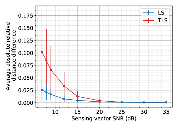
Refer to caption
Figure 12: The average of the absolute value difference between the actual relative distance and the relative error reconstruction from Proposition 3 when MN=8𝑀𝑁8\frac{M}{N}=8. Measurement SNR is twice the sensing vector SNR.

Appendix F Handcrafted errors

Using the results and notation of Section III, we show that there exist error models which can significantly change the relative performance of TLS and LS. With scalars ka,ky+subscript𝑘𝑎subscript𝑘𝑦superscriptk_{a},\,k_{y}\in\mathbb{R}^{+} to control the SNR of 𝑬𝑨subscript𝑬𝑨\bm{{E}}_{\bm{{A}}} and 𝑬𝒀subscript𝑬𝒀\bm{{E}}_{\bm{{Y}}}, we create errors 𝑬𝑨=ka𝑫1𝑬𝑨subscript𝑬𝑨subscript𝑘𝑎superscript𝑫1superscriptsubscript𝑬𝑨\bm{{E}}_{\bm{{A}}}=k_{a}\bm{{D}}^{-1}\bm{{E}}_{\bm{{A}}}^{\prime} for some 𝑬𝑨superscriptsubscript𝑬𝑨\bm{{E}}_{\bm{{A}}}^{\prime} and 𝑬𝒀=ky𝑫1𝑬𝒀subscript𝑬𝒀subscript𝑘𝑦superscript𝑫1superscriptsubscript𝑬𝒀\bm{{E}}_{\bm{{Y}}}=k_{y}\bm{{D}}^{-1}\bm{{E}}_{\bm{{Y}}}^{\prime} for some diagonal 𝑬𝒀superscriptsubscript𝑬𝒀\bm{{E}}_{\bm{{Y}}}^{\prime}. With these errors, the expressions from Proposition 3 become

eTLSsubscript𝑒TLS\displaystyle e_{\mathrm{TLS}} =(𝑨~T𝒀~𝑫𝑨~)1𝑨~T𝒀~𝒘2absentsubscriptdelimited-∥∥superscriptsuperscript~𝑨𝑇~𝒀𝑫~𝑨1superscript~𝑨𝑇~𝒀superscript𝒘2\displaystyle=\left\lVert\left(\widetilde{\bm{{A}}}^{T}\widetilde{\bm{{Y}}}\bm{{D}}\widetilde{\bm{{A}}}\right)^{-1}\widetilde{\bm{{A}}}^{T}\widetilde{\bm{{Y}}}\bm{{w}}^{\prime}\right\rVert_{2} (125)
eLSsubscript𝑒LS\displaystyle e_{\mathrm{LS}} =(𝑨~T𝒀~𝑨~)1𝑨~T𝒀~𝑫1𝒘2absentsubscriptdelimited-∥∥superscriptsuperscript~𝑨𝑇~𝒀~𝑨1superscript~𝑨𝑇~𝒀superscript𝑫1superscript𝒘2\displaystyle=\left\lVert\left(\widetilde{\bm{{A}}}^{T}\widetilde{\bm{{Y}}}\widetilde{\bm{{A}}}\right)^{-1}\widetilde{\bm{{A}}}^{T}\widetilde{\bm{{Y}}}\bm{{D}}^{-1}\bm{{w}}^{\prime}\right\rVert_{2} (126)

where 𝒘=((2𝒀~)1ky𝑬𝒀𝑨~ka𝑬𝑨)𝒙#superscript𝒘superscript2~𝒀1subscript𝑘𝑦superscriptsubscript𝑬𝒀~𝑨subscript𝑘𝑎superscriptsubscript𝑬𝑨superscript𝒙#\bm{{w}}^{\prime}=((2\widetilde{\bm{{Y}}})^{-1}k_{y}\bm{{E}}_{\bm{{Y}}}^{\prime}\widetilde{\bm{{A}}}-k_{a}\bm{{E}}_{\bm{{A}}}^{\prime})\bm{{x}}^{\#}. Compared to (45), eTLSsubscript𝑒TLSe_{\mathrm{TLS}} in (125) does not multiply 𝒘superscript𝒘\bm{{w}}^{\prime} by 𝑫𝑫\bm{{D}}. Additionally, compared to (46), eLSsubscript𝑒LSe_{\mathrm{LS}} in (126) multiplies 𝒘superscript𝒘\bm{{w}}^{\prime} by 𝑫1superscript𝑫1\bm{{D}}^{-1}. The elements of diagonal matrix 𝑫1superscript𝑫1\bm{{D}}^{-1} are greater than one, dmm1=(1+4λyλa𝒙#22y~m)>1subscriptsuperscript𝑑1𝑚𝑚14subscript𝜆𝑦subscript𝜆𝑎superscriptsubscriptdelimited-∥∥superscript𝒙#22subscript~𝑦𝑚1d^{-1}_{mm}=\left(1+\frac{4\lambda_{y}}{\lambda_{a}}\left\lVert\bm{{x}}^{\#}\right\rVert_{2}^{2}\widetilde{y}_{m}\right)>1, and we investigate how this alters performance when the sensing vectors follow the iid standard real Gaussian measurement model. Appendix G-A contains experiments using the coded diffraction pattern model.

F-A First-order reconstruction error numerical experiments

In the next set of experiments, 𝑬𝑨=ka𝑫11𝑬𝑨subscript𝑬𝑨subscript𝑘𝑎superscriptsubscript𝑫11superscriptsubscript𝑬𝑨\bm{{E}}_{\bm{{A}}}=k_{a}\bm{{D}}_{1}^{-1}\bm{{E}}_{\bm{{A}}}^{\prime} and 𝑬𝒀=ky𝑫11𝑬𝒀subscript𝑬𝒀subscript𝑘𝑦superscriptsubscript𝑫11superscriptsubscript𝑬𝒀\bm{{E}}_{\bm{{Y}}}=k_{y}\bm{{D}}_{1}^{-1}\bm{{E}}_{\bm{{Y}}}^{\prime}, where 𝑫1=(𝑰M+4𝒙#22𝒀~)1subscript𝑫1superscriptsubscript𝑰𝑀4superscriptsubscriptdelimited-∥∥superscript𝒙#22~𝒀1\bm{{D}}_{1}=(\bm{{I}}_{M}+4\left\lVert\bm{{x}}^{\#}\right\rVert_{2}^{2}\widetilde{\bm{{Y}}})^{-1} is free of the regularization parameters. Matrix 𝑬𝑨superscriptsubscript𝑬𝑨\bm{{E}}_{\bm{{A}}}^{\prime} and diagonal matrix 𝑬𝒀superscriptsubscript𝑬𝒀\bm{{E}}_{\bm{{Y}}}^{\prime} are iid zero-mean Gaussian. We repeat the experiment of Fig. 2b using these created errors in Fig. 13. All other experimental details are unchanged. We see that now TLS outperforms LS with this error model.
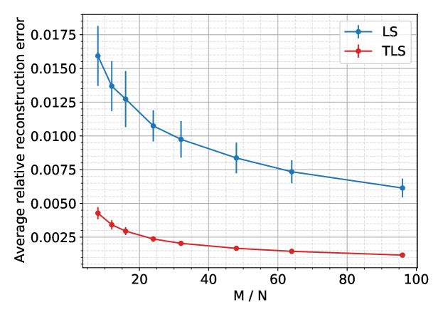
Refer to caption
Figure 13: Relative reconstruction errors, (45) and (46) for different values of MN𝑀𝑁\frac{M}{N} when handcrafted errors are used. Measurement and sensing vector SNRs are 40 dB.

Next we fix MN=8𝑀𝑁8\frac{M}{N}=8 and the sensing vector SNR to 100 dB so there is virtually no sensing vector error. We vary the measurement SNR over 100 trials and use the handcrafted errors. The sensing vectors and ground truth signals are generated in the same way as in the numerical experiments of Section III. In Fig. 14 we plot the average first-order relative reconstruction error and see that with this setting TLS outperforms LS. This occurs despite there only being measurement error, a setting where we may expect LS to outperform TLS.

The results in Figs. 13 and 14 show that the type of measurement and sensing vector error can impact performance.
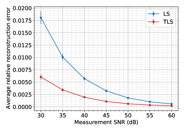
Refer to caption
Figure 14: Relative reconstruction errors with handcrafted errors when there is only error in measurements. Here MN=8𝑀𝑁8\frac{M}{N}=8.

F-B Simulations with actual reconstruction error

To investigate the impact of this error model on the actual reconstruction error, we design handcrafted errors in the same manner as above and calculate the actual reconstruction error. Despite the earlier analysis using real-valued errors, we show that the ideas carry through when we use the complex Gaussian measurement model with 𝑬𝑨subscript𝑬𝑨\bm{{E}}_{\bm{{A}}} being complex Gaussian.

In the first simulation we use a step size of 0.5λa0.5subscript𝜆𝑎\frac{0.5}{\lambda_{a}} for TLS and 0.02 for LS and repeat the experiment of Fig. 5b with handcrafted errors instead. Fig. 15 shows that in this setting TLS outperforms LS, the opposite of what is seen with Gaussian errors in Fig. 5b. This is consistent with the first-order reconstruction error numerical experiment of Fig. 13.
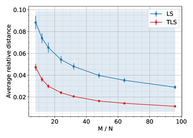
Refer to caption
Figure 15: Relative distance of reconstructions using TLS and LS for the Gaussian measurement model for different values of MN𝑀𝑁\frac{M}{N} when handcrafted errors are used. Measurement SNR is 20 dB and sensing vector SNR is 30 dB.

Next we use MN=8𝑀𝑁8\frac{M}{N}=8 and a step size of 0.2λa0.2subscript𝜆𝑎\frac{0.2}{\lambda_{a}} for TLS and 0.02 for LS. Following the experiment of Fig. 14, in Fig. 16 the sensing vector SNR is 100 dB and there is virtually no sensing vector error. The measurement SNR is varied and the performance of TLS and LS with handcrafted errors is compared to TLS and LS with iid Gaussian errors. We do 100 trials at each measurement SNR. Even though there is significant error only in the measurements, TLS with handcrafted errors outperforms LS as was suggested by Fig. 14. With Gaussian errors, LS outperforms TLS when there are only measurement errors.
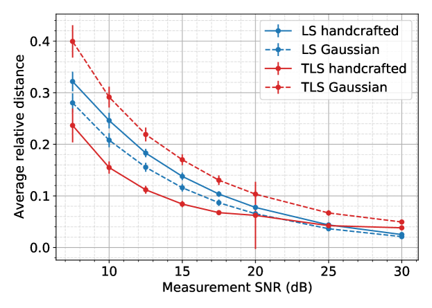
Refer to caption
Figure 16: Performance of TLS and LS with handcrafted errors when there is only error in measurements for the Gaussian measurement model. Here MN=8𝑀𝑁8\frac{M}{N}=8.

With MN=8𝑀𝑁8\frac{M}{N}=8 and handcrafted errors, Fig. 17 shows an identical experiment to that of Fig. 4. We see that the relative performance of TLS over LS improves with handcrafted errors compared to Fig. 4 where random Gaussian errors were used.
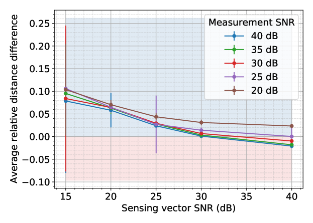
Refer to caption
Figure 17: Average difference in relative distance between TLS and LS solutions for the Gaussian measurement model when MN=8𝑀𝑁8\frac{M}{N}=8 for different measurement and sensing vector SNR combinations when the errors are handcrafted. This can be compared to Fig. 4 when MN=8𝑀𝑁8\frac{M}{N}=8.

Appendix G Coded diffraction pattern (CDP) measurement model

Denoting row n𝑛n of the N𝑁N-point DFT matrix as 𝒇nsuperscriptsubscript𝒇𝑛\bm{{f}}_{n}^{*} and L𝐿L modulation patterns {𝒑l}l=1LNsuperscriptsubscriptsubscript𝒑𝑙𝑙1𝐿superscript𝑁\{\bm{{p}}_{l}\}_{l=1}^{L}\in\mathbb{C}^{N}, the M=LN𝑀𝐿𝑁M=LN quadratic coded diffraction pattern measurements are then

ym|𝒇ndiag(𝒑l)𝒂m𝒙|2,m=(n,l)formulae-sequencesubscript𝑦𝑚superscriptsubscriptsuperscriptsubscript𝒇𝑛diagsuperscriptsubscript𝒑𝑙superscriptsubscript𝒂𝑚𝒙2𝑚𝑛𝑙\displaystyle y_{m}\approx|\underbrace{\bm{{f}}_{n}^{*}\mathop{\mathrm{diag}}(\bm{{p}}_{l})^{*}}_{\bm{{a}}_{m}^{*}}\bm{{x}}|^{2},\qquad m=(n,l) (127)

where 1nN1𝑛𝑁1\leq n\leq N, 1lL1𝑙𝐿1\leq l\leq L [41]. The modulation patterns 𝒑lNsubscript𝒑𝑙superscript𝑁\bm{{p}}_{l}\in\mathbb{C}^{N} follow the octanary pattern which means its entries are iid and follow the distribution of p𝑝p where p=q1q2𝑝subscript𝑞1subscript𝑞2p=q_{1}q_{2}. The random variable q1subscript𝑞1q_{1} is one of {1,1,j,j}11𝑗𝑗\{-1,1,-j,j\} with equal probability and q2=22subscript𝑞222q_{2}=\frac{\sqrt{2}}{2} with probability 0.8 or q2=3subscript𝑞23q_{2}=\sqrt{3} with probability 0.2. Note that M𝑀M can only be an integer multiple of N𝑁N and depends on the number of patterns used.

G-A Experiments

In this section we repeat the experiments that were done for the Gaussian measurement model in Section IV for the CDP measurement model. The experimental setup such as the number of trials, type of ground truth signal, step sizes and iteration stopping criteria are the same as those used for the equivalent simulation with the Gaussian model.

Random errors

The experiments in Figs. 18, 19a, 19b are for the CDP measurement model and are the same as Figs. 4, 5a and 5b for the Gaussian measurement model.
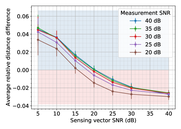
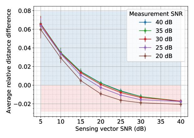
Refer to caption
(a) L=MN=16𝐿𝑀𝑁16L=\frac{M}{N}=16
Refer to caption
(b) L=MN=32𝐿𝑀𝑁32L=\frac{M}{N}=32
Figure 18: Average difference in relative distance of TLS and LS solutions, rel.dist(𝒙#,𝒙LS)rel.dist(𝒙#,𝒙TLS)formulae-sequencereldistsuperscript𝒙#subscriptsuperscript𝒙LSreldistsuperscript𝒙#subscriptsuperscript𝒙TLS\mathrm{rel.dist}(\bm{{x}}^{\#},\bm{{x}}^{\dagger}_{\mathrm{LS}})-\mathrm{rel.dist}(\bm{{x}}^{\#},\bm{{x}}^{\dagger}_{\mathrm{TLS}}), for the octanary CDP measurement model for different measurement and sensing vector SNR combinations when the number of patterns is L=MN{16,32}𝐿𝑀𝑁1632L=\frac{M}{N}\in\{16,32\}.
Refer to caption
(a) Sensing vector SNR is 10 dB. Gaussian errors.
Refer to caption
(b) Sensing vector SNR is 30 dB. Gaussian errors.
Refer to caption
(c) Sensing vector SNR is 30 dB. Handcrafted errors.
Figure 19: Relative distance of reconstructions using TLS and LS for the CDP measurement model for different number of patterns L=MN𝐿𝑀𝑁L=\frac{M}{N} when measurement SNR is 20 dB.

Handcrafted errors

Figs. 19c, 20 and 21 show the performance with handcrafted errors for the CDP measurement model. With only handcrafted measurement error and 100 dB SNR sensing vector error, the performance of TLS is better than LS for low measurement SNR in Fig. 20 compared to when there are random Gaussian errors. The performance with different error combinations for handcrafted errors in Fig. 21 should be compared against Fig. 18.
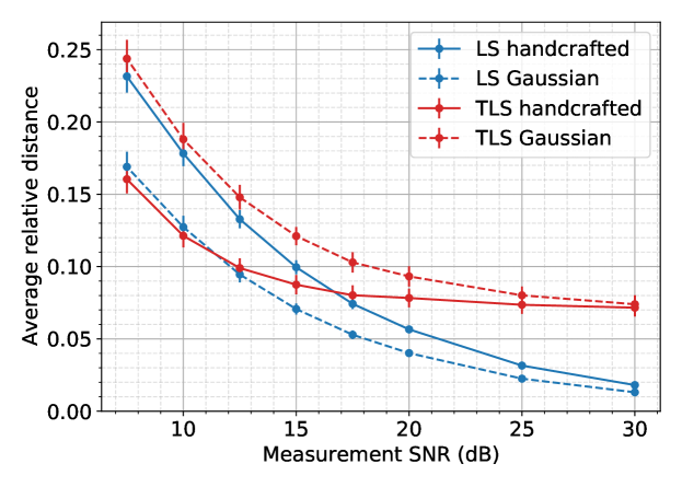
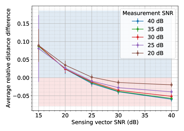
Refer to caption
Figure 20: Performance of TLS and LS with handcrafted errors when there is only error in measurements for the CDP measurement model. Here L=MN=16𝐿𝑀𝑁16L=\frac{M}{N}=16 octanary patterns are used.
Refer to caption
Figure 21: Average difference in relative distance between TLS and LS solutions for the CDP measurement model when L=MN=16𝐿𝑀𝑁16L=\frac{M}{N}=16 octanary patterns are used. Different measurement and sensing vector SNR combinations are used and the errors are handcrafted. This should be compared to Fig. 18 when L=MN=16𝐿𝑀𝑁16L=\frac{M}{N}=16.

Sensing vector correction verification

The experiments done to verify the sensing vector corrections for the Gaussian measurement model in Figs. 6 and 7 are done for the CDP measurement model in Figs. 22 and 23.
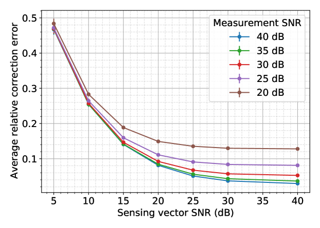
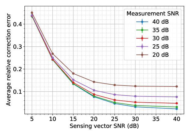
Refer to caption
(a) L=MN=16𝐿𝑀𝑁16L=\frac{M}{N}=16
Refer to caption
(b) L=MN=32𝐿𝑀𝑁32L=\frac{M}{N}=32
Figure 22: Average relative sensing vector correction error when using TLS, rel.corr({𝒂~,𝒙#},{𝒂^,ejφ𝒙TLS)\mathrm{rel.corr}(\{\widetilde{\bm{{a}}},\,\bm{{x}}^{\#}\},\{\widehat{\bm{{a}}}^{\dagger},\,\mathrm{e}^{j\varphi}\bm{{x}}^{\dagger}_{\mathrm{TLS}}), for the CDP measurement model for different measurement and sensing vector SNR combinations when the number of patterns is L=MN{16,32}𝐿𝑀𝑁1632L=\frac{M}{N}\in\{16,32\}.
Refer to caption
Figure 23: Relative sensing vector correction error when using TLS for the CDP measurement model for different number of patterns L=MN𝐿𝑀𝑁L=\frac{M}{N} when measurement SNR is 20 dB. The sensing vector SNR is 10 dB or 30 dB.

Appendix H Additional OPU experiment information

H-A Sensing vector calibration

Sensing vector calibration is typically time consuming due to the quadratic nature of (1). We use a rapid numerical interferometry calibration procedure that first inputs K𝐾K calibration signals, 𝚵=[𝝃1,,𝝃K]N×K𝚵subscript𝝃1subscript𝝃𝐾superscript𝑁𝐾\bm{{\Xi}}=[\bm{{\xi}}_{1},\ldots,\bm{{\xi}}_{K}]\in\mathbb{R}^{N\times K} into the OPU and obtains the phase of the corresponding optical measurements, 𝑺𝑺\bm{{S}} in 𝑸:=|𝑺|2|𝑨𝚵|2M×Kassign𝑸superscript𝑺2superscript𝑨𝚵2superscript𝑀𝐾\bm{{Q}}:={\left|\bm{{S}}\right|}^{2}\approx{\left|\bm{{A}}\bm{{\Xi}}\right|}^{2}\in\mathbb{R}^{M\times K}. Transmission matrix 𝑨M×N𝑨superscript𝑀𝑁\bm{{A}}\in\mathbb{C}^{M\times N} is then recovered by solving the linear system 𝑺=𝑨𝚵𝑺𝑨𝚵\bm{{S}}=\bm{{A}}\bm{{\Xi}} [2]. If 𝑺𝑺\bm{{S}} has errors, the calibrated 𝑨𝑨\bm{{A}} may have errors. We implemented this method with 1.5N1.5𝑁1.5N calibration signals and 20 anchor signals. We use the same procedure as Gupta et al. to design calibration signals [2].

H-B Experiment details

When doing the experiments with random images on the OPU, we set the camera exposure time to 700 μs𝜇𝑠\mu s to utilize and not saturate the full zero to 255 8-bit measurement range of the camera. The input display frametime is set to 1200 μs𝜇𝑠\mu s. For the experiments with the real images, the camera exposure is 400 μs𝜇𝑠\mu s and the frametime is 500 μs𝜇𝑠\mu s.

To use a new set of sensing vectors in each trial we calibrate a complex-valued transmission matrix with 217superscript2172^{17} rows. In each trial in Fig. 9 we then do phase retrieval by choosing a new set of M𝑀M rows. The optical measurements corresponding to the chosen M𝑀M rows are used. As previously, the TLS and LS iterations in Algorithm 1 are stopped when the objective function value between successive iterates changes by less than 106superscript10610^{-6} and the initialization is done using 50 iterations of the power method.

Because the output device exposure time controls the range of the measurements, the entries of the calibrated OPU transmission matrix are iid complex Gaussian and the calibrated Gaussian sensing vectors are scaled versions of the sensing vectors from the complex Gaussian measurement model. This does not impact the sensing vector updates in Section II-B because the procedure does not assume a measurement model. However, the initialization scaling and signal gradient descent updates (7) for both TLS and LS require minor changes. Instead of altering these steps we estimate the standard deviation and variance of the calibrated transmission matrix from its entries and divide the calibrated matrix by the estimated standard deviation. Correspondingly, we also divide the measurements by the estimated variance.