On the periodicity of cardiovascular fluid dynamics simulations
Abstract
Three-dimensional cardiovascular fluid dynamics simulations typically require computation of several cardiac cycles before they reach a periodic solution, rendering them computationally expensive. Furthermore, there is currently no standardized method to determined whether a simulation has yet reached that periodic state. In this work, we propose use of the asymptotic error measure to quantify the difference between simulation results and their ideal periodic state using lumped-parameter modeling. We further show that initial conditions are crucial in reducing computational time and develop an automated framework to generate appropriate initial conditions from a one-dimensional model of blood flow. We demonstrate the performance of our initialization method using six patient-specific models from the Vascular Model Repository. In our examples, our initialization protocol achieves periodic convergence within one or two cardiac cycles, leading to a significant reduction in computational cost compared to standard methods. All computational tools used in this work are implemented in the open-source software platform SimVascular. Automatically generated initial conditions have the potential to significantly reduce computation time in cardiovascular fluid dynamics simulations.
1 Introduction
Three-dimensional (3D) blood flow simulations are commonly coupled with zero-dimensional (0D) lumped parameter models, representing the downstream vasculature at the model’s boundary [1, 2, 3, 4]. These lumped parameter models are analogous to an electric circuit, with resistors and capacitors modeling the viscosity of the blood and the elasticity of the vessel wall, respectively. A popular choice is the three-element Windkessel model, also known as the RCR model [5]. The Windkessel consists of a proximal resistance in series with a parallel distal resistance and capacitance (Figure 1).
The RCR boundary condition, like many other outflow boundary conditions, contains a capacitor that stores blood volume. While these capacitors are “charging”, it typically takes several cardiac cycles with a periodic pulsatile inflow to reach a periodic state. A periodic state is here defined as two consecutive cardiac cycles yielding results for pressure and flow rate that agree within a given tolerance. Mathematically, this corresponds to the limit cycle of the model. It is essential to extract simulation results only when they have reached this periodic state, e.g., when comparing them to in vivo measurements. However, there are currently no clear guidelines on how to determine whether this periodic state has been achieved.
Unfortunately, running several cardiac cycles of a 3D simulation is computationally expensive, typically requiring a high-performance computer. The computation time scales linearly with the number of cardiac cycles since they cannot be run in parallel. A common practice is initializing a simulation with results from a steady-state solution [5]. Here, a computationally inexpensive simulation with constant inflow is computed first. Its solution is then used as an initial condition for the simulation with a periodic pulsatile inflow condition. However, as we will show in this work, a simulation initialized with a steady-state solution often still requires several cardiac cycles to reach a reasonably periodic state.
Our goal is twofold. First, we introduce metrics and tools to quantify whether a simulation has yet reached a periodic state within a given tolerance. Second, we shorten the computation time of the computationally expensive 3D simulation by leveraging reduced-order modeling. It was previously shown that one-dimensional (1D) models of cardiovascular fluid dynamics could accurately approximate integral quantities of 3D solutions such as velocity and pressure at the outlets [6, 7, 8, 9, 10, 11, 12]. In this work, we propose a novel method to initialize a 3D simulation using the results from an inexpensive 1D simulation. This framework is fully automated and requires no user interaction.
2 Methods
We begin by revisiting the governing equations of 3D, 1D, and 0D fluid dynamics in Sections 2.1, 2.2, and 2.3. Following theoretical considerations of the convergence of lumped parameter models, we define suitable error metrics to determine the difference between a 3D simulation and its periodic state in Section 2.4. In Section 2.5, we introduce a tool to determine whether a simulation has yet reached its periodic state. Finally, we develop a method to initialize a 3D simulation from a 1D simulation in Section 2.6 in order to jumpstart initialization and reduce computational cost.
2.1 3D flow physics
The dynamics of blood flow in the cardiovascular system is mathematically governed by the incompressible 3D Navier-Stokes equations,
| in | (1) | |||||
| in | (2) |
The first equation in this system represents conservation of momentum for a Newtonain, incompressible fluid, where is the velocity of the blood flow, is pressure, is a body force, is the density of the blood, and is the dynamic viscosity. The second equation in this system represents conservation of mass. In the computational cardiovascular modeling and simulation context, we typically numerically solve the 3D Navier-Stokes equations in patient-specific models of vascular anatomies to simulate hemodynamics. Simulation results are used to elucidate the relationship between cardiovascular diseases and fluid mechanics, for personalized treatment planning, and to aid the development of novel biomedical technologies. The initial conditions for velocity and pressure are
| (3) |
Boundary conditions that model the portion of the cardiovascular system not captured by the anatomical model must be provided as well. A flow rate, , is commonly prescribed at the inlet surfaces of the 3D vascular model, where the flow rate is computed via integration of the normal velocity over each inlet surface,
| in | (4) |
On the other hand, lumped parameter models, also known as 0D models, are commonly used as boundary conditions at the outlets of the model. These lumped parameter models usually relate the pressure to the flow rate via parametric differential-algebraic equations,
| on | (5) |
where represents the set of variables parametrizing the differential equation. A discussion of 0D models and some commonly used outlet boundary conditions is provided in section 2.3.
We generate 3D patient-specific models using SimVascular, an open-source, comprehensive modeling, and simulation software for vascular anatomies (simvascular.org) [13]. The models are simulated in our open-source solver svSolver using the Finite Element Method (FEM) (github.com/SimVascular/svSolver). It uses liner P1-P1 elements with a streamline upwind Petrov-Galerkin and pressure-stabilizing Petrov-Galerkin formulation (SUPG/PSPG) [14]. The pressure and momentum stabilization is detailed in [15, 16]. Furthermore, it uses a linear solver with specialized pre-conditioners tailored to handle large vascular resistances coupled at outflow boundaries [17]. All 3D simulations in this work were run on Stanford’s Sherlock supercomputing cluster using four 12-core Intel Xeon Gold 5118 CPUs.
2.2 1D flow physics
In contrast to 3D models, one-dimensional (1D) models have only a single spatial dimension, the axial dimension along the centerline of the vessel [18, 6, 19]. Due to this lack of 3D spatial information, 1D models are capable of simulating only bulk flow rate, and cross-sectionally averaged pressure at each centerline node of the 1D finite element model. We integrate incompressible 3D Navier-Stokes equations (1) over the cross-section while assuming Newtonian fluid properties for the blood and an axisymmetric parabolic flow profile to obtain the governing equations for the 1D model. This process yields
| (6) | ||||
| (7) |
with flow rate , cross-sectional area , pressure , density , body force , and kinematic viscosity . The coordinate represents the axial dimension of 1D model. To solve these equations, we also require a constitutive law to relate the pressure to the cross-sectional area. In this work, we use the constitutive relationship proposed by Olufsen [20],
| (8) |
where is the Young’s modulus of the blood vessel, is the wall thickness, is the reference pressure, is the reference radius, and , , and are empirically derived constants.
Furthermore, for models with multiple vascular branches, mass conservation is obeyed at the junction regions, and the pressure is assumed to be constant between the inlet and outlets of the junctions [6]. As with 3D models, we need initial conditions to initialize the simulation,
| (9) |
as well as inlet and outlet boundary conditions, discussed in section 2.3, to represent the portion of the cardiovascular not reflected in our 1D model,
| in | (10) | |||||
| in | (11) |
We generate and simulate the 1D centerline and finite element models using SimVascular and VMTK [21]. We solve the set of differential equations using our open-source solver svOneDSolver (github.com/SimVascular/svOneDSolver). We employ a stabilized space-time finite element method based on the discontinuous Galerkin method in time [6]. The spatial discretization employs continuous piecewise linear polynomials whereas we use a piecewise constant temporal discretization. For more background information, see [22, 23, 24].
2.3 0D flow physics
The third model fidelity we consider in this work is the zero-dimensional (0D) model. Unlike 3D and 1D models, 0D models lack spatial information. However, as with 1D models, 0D models are capable of accurately simulating bulk flow rate and bulk pressure quantities in the cardiovascular system [25], [26]. These 0D models are composed of individual lumped-parameter elements that connect to form an entire complex lumped parameter network. There are many lumped parameter elements commonly used in the context of cardiovascular modeling and simulation. Some of these elements include resistors, capacitors, and inductors [26]. Resistors model the viscous effects of blood flow, capacitors represent the elastic nature of blood vessels, while inductors capture the inertia of the blood flow. In lumped parameter networks that model the heart, diode elements are also employed. These diodes mimic the behavior of heart valves, where they allow flow to pass only when the valves are open [27], [28]. The flow rates and pressures in each of these elements are respectively governed by the following linear differential and algebraic equations,
| (12) |
where is the resistance, is the capacitance, is the inductance, and is the pressure drop across the element. Lumped parameter 0D models are also analogous to electrical circuits, where the flow rate and pressure are representative of current and voltage, respectively. In this work, we will focus our attention to just resistors and capacitors.
Lumped parameter networks are commonly used in two contexts. First, 0D models can be used as surrogate models of entire vascular anatomies [25]. In this case, each blood vessel in the vascular system is represented by one or more lumped-parameter elements in the 0D model, where the value of each element is determined by the geometric and material properties of the blood and blood vessel. Second, 0D models can be used to represent boundary conditions in 3D and 1D models [27], [29], [17], [30], [31]. In this context, each 0D element reflects a different downstream (or upstream) anatomical feature of the cardiovascular system. To employ the 0D models as boundary conditions, they must be numerically coupled to the 3D or 1D finite element models [17]. The governing equations for these 0D models then can be numerically solved using traditional time-stepping schemes, such as an explicit fourth-order Runge-Kutta method.
Some of the 0D models most commonly employed as boundary conditions are the resistance model and the 3-element Windkessel model [5, 31]. The resistance model is composed of a single linear resistor element that captures the downstream resistance of the vascular network not portrayed in the 3D or 1D model. On the other hand, the 3-element Windkessel model, also known as the RCR model, as shown in Figure 1, models the proximal resistance, distal resistance, and compliance of the downstream vasculature using two resistor elements and a capacitor. The RCR boundary condition is discussed further in the next section.
To simulate our 0D surrogate models, which represent the vessels using linear resistors, we solve the governing system of equations using an in-house, modular numerical solver that employs the implicit generalized- scheme for time advancement [32].
2.4 The RCR boundary condition
Thus far, we have introduced three different model fidelities commonly used in computational vascular modeling and simulation. Before any of the models and simulation results can be used in predictive and scientific applications, the quantities of interest, primarily the flow rates and pressures, must be simulated until they converge to a periodic state. Here, a simulated quantity of interest is considered to be periodic if its values between 2 adjacent periods are the same, within some defined tolerance. A period in the cardiovascular context is typically defined as a single cardiac cycle. We expound on the concept of a periodic state in this section, using the RCR model to illustrate the primary concepts.
The three parameters of the RCR boundary condition are commonly tuned to clinical measurements, i.e., phase-contrast magnetic resonance imaging and pressure measurements by solving an optimization problem to match minimal and maximal pressure over a cardiac cycle, measured flows, and flow distribution among different outlets [33]. A common strategy is to tune the total resistance and capacitance in the model to produce a physiologic pressure waveform, then distributed proportional to the vessel outlet areas [34].
We begin by reviewing the response of a single RCR model to pulsatile inflow. The governing differential equation for the inlet pressure, , of the 3-element Windkessel model, as a function of the inlet flow rate, , is
| (13) |
where is the proximal resistance, is the capacitance, and is the distal resistance. We obtain the semi-analytical solution [29] for this ordinary differential equation as
| (14) |
which depends on the inflow and the time constant . We can identify three different terms in this equation: (I) exponential decay of the initial solution, (II) pressure drop at proximal resistance, (III) pressure drop at sub-circuit . Assuming a constant inflow for , we obtain the pressure step response for the RCR boundary condition as
| (15) |
starting at the initial pressure and exponentially approaching the asymptotic pressure for the limit . We now define the periodic inflow as
| (16) |
where the period is the length of a cardiac cycle and the time-averaged mean flow. The mean pressure in the -th cardiac cycle is denoted by
| (17) |
With this notation, Equation (15) can be reformulated for a non-constant, periodic pulsatile inflow as
| (18) |
starting at the initial mean pressure and approaching the asymptotic mean pressure . Note that the asymptotic mean pressure can in general not be determined analytically but depends on the function . Notably, is different from the asymptotic pressure that approaches for a solution with steady mean flow .
In the remainder of this section, we will define an error metric to quantify the difference between the pressure in the -th cardiac cycle and the asymptotic pressure . For simplicity of notation, we show the following derivations for , i.e. the pressure approaches the asymptotic pressure “from below”. However, the conclusions hold for any choice of initial pressure. We define the asymptotic error as
| (19) |
Thus, we can calculate the number of cardiac cycles required for the RCR boundary condition to reach a periodic state within the tolerance as
| (20) |
Several observations can be made from Equation (20). First, the number of cycles scales linearly with , the ratio of the length of the time constant to the length of one cardiac cycle. A two-fold increase in the time constant doubles the number of cardiac cycles required to reach the same tolerance . Second, the closer the initial pressure to the asymptotic pressure the fewer cardiac cycles are required to achieve periodic convergence with an error . The error and the number of cardiac cycles can in general not be determined a priori since the constant cannot be evaluated analytically. Only in the special case of starting from zero initial conditions, i.e. , the number of cardiac cycles to periodic convergence can be directly given as
| (21) |
We can easily compute the difference between two cardiac cycles numerically without the solution having reached a periodic state. Using this difference, we define the cyclic error between two consecutive cardiac cycles as
| (22) |
We then define the ratio between asymptotic error and cyclic error as
| (23) |
Equation (23) shows that in general . While error metrics like are commonly used in practice to determine whether a simulation as reached a periodic state within a given tolerance, it is not an adequate metric to do so. For time constants larger than 1.44 times the length of the cardiac cycle , the cyclic error will underestimate the asymptotic error . In simulations with a large time constant the error will appear small despite the solution being far from a periodic state due to their slow convergence. As a remedy, we propose a method in Section 2.5 to estimate the asymptotic error as the simulation is being computed.
2.5 Checking the periodicity of 3D simulations
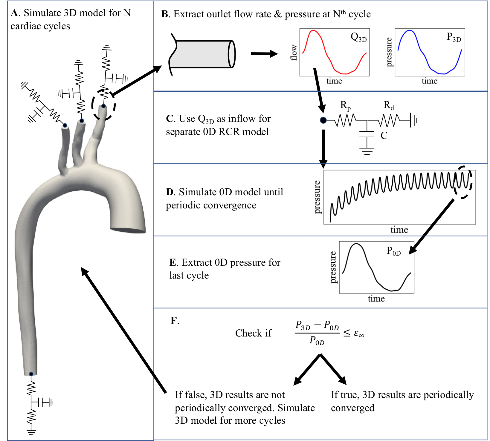
The previous section introduced analytical and theoretical methods to check the periodicity of a single RCR model subjected to a prescribed inflow condition. This section extends this discussion to consider computational vascular models and present a method to check the periodicity of patient-specific, multi-outlet 3D models, where each outlet is coupled to a different RCR boundary condition. The steps for this method are summarized in the flowchart shown in Figure 1.
As mentioned in the previous section, generally cannot be predicted analytically. However, a value of is needed to check if the simulated flow rate and pressure at each outlet of the 3D model have converged to a periodic state. To remedy this issue, we estimate for each outlet by simulating a separate 0D model of the attached RCR boundary condition. The inflow to each 0D RCR model is the simulated 3D flow rate, , corresponding to that outlet. We then simulate these simple 0D RCR models for many cardiac cycles, to guarantee periodic convergence of the 0D RCR model, and use the final simulated pressure values, , as our estimates of .
Furthermore, as previously discussed, represents the asymptotic error of the pressure solution. We therefore specify a desired value for and use this as our criteria for periodic convergence. Our 3D pressure solution, , is considered to be periodically converged, as per Equation (19), if it matches within this error threshold. Mathematically, this condition is expressed as,
| (24) |
Note that should be reasonably close to a periodic state before we can use it as the inflow to our RCR model. Typically, converges much faster, i.e., within one or two cardiac cycles, than does. This note will be further discussed in Section 3.1.3.
Lastly, each outlet of our 3D models has in general a unique time constant . Although, in practice, parameter tuning yields time constants that are similar. It can be shown that the convergence of each outlet is determined by a single model time constant that can be approximated by the mean of all individual time constants. As such, we can use this average time constant to estimate the number of cardiac cycles for which our 3D models must be simulated to achieve periodic convergence.
2.6 Generating initial conditions
As previously discussed, 3D models must be simulated until the flow rates and pressures converge to a periodic state before they can be applied in scientific or clinical investigations, which currently requires running the simulation for several cardiac cycles. This limits the utility of computational 3D models and simulations in real-world clinical applications. To alleviate this bottleneck, we introduce a novel method to jumpstart the initialization of 3D simulations. In particular, we generate initial conditions to minimize the number of cardiac cycles required to reach periodic convergence within a chosen tolerance. This process is fully automated in SimVascular [13] and requires no user input. Starting from a periodic 1D solution (Section 2.6.1) we create a map from the centerline, the 1D representation of the model, to the 3D volume mesh (Section 2.6.2), and generate an artificial initial velocity vector field (Section 2.6.3) for simulation initialization.
2.6.1 Generating a periodic 1D solution
We automatically generate a 1D flow model of the high-fidelity 3D flow model using the SimVascular 1D-plugin. We then run the model until it achieves periodic convergence and extract the solution of the last cardiac cycle.
2.6.2 Mapping centerline to volume mesh
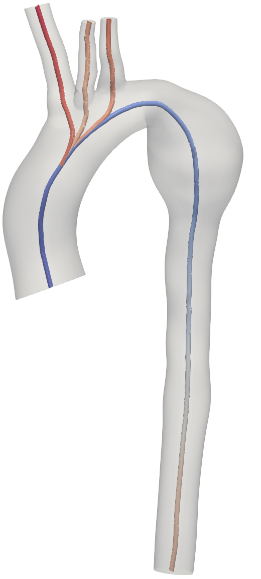
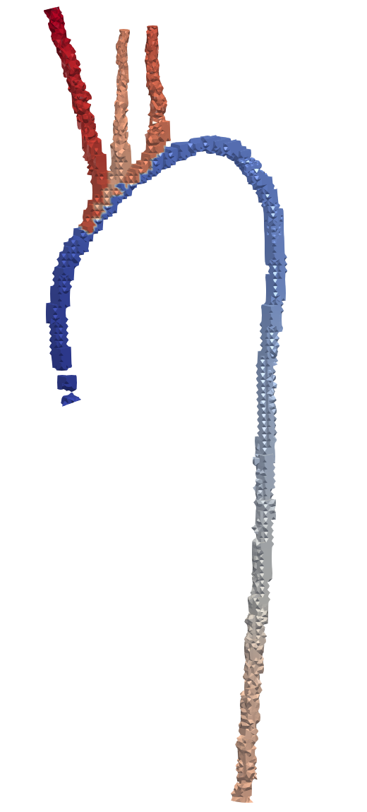
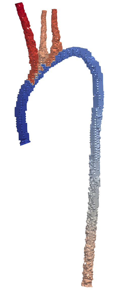
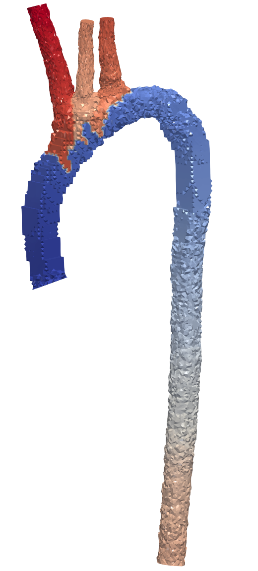
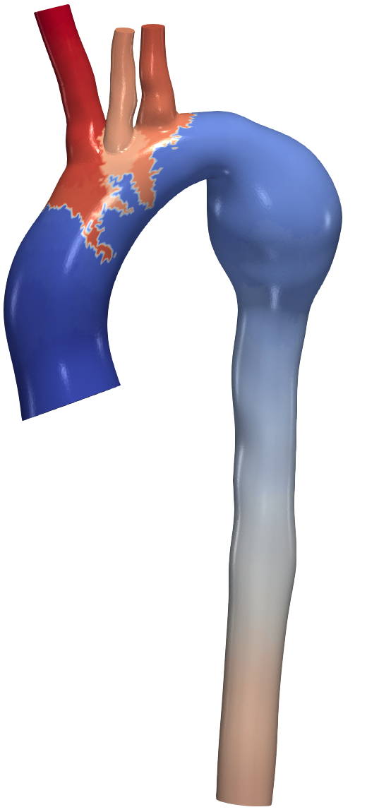
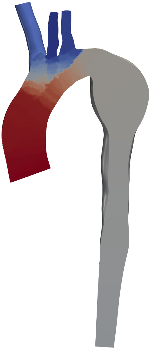
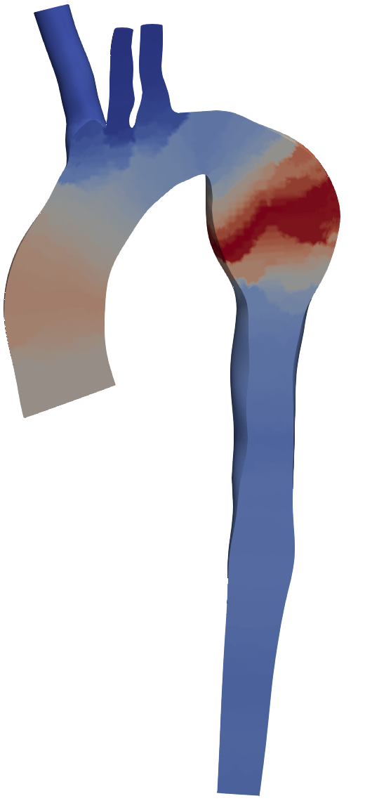
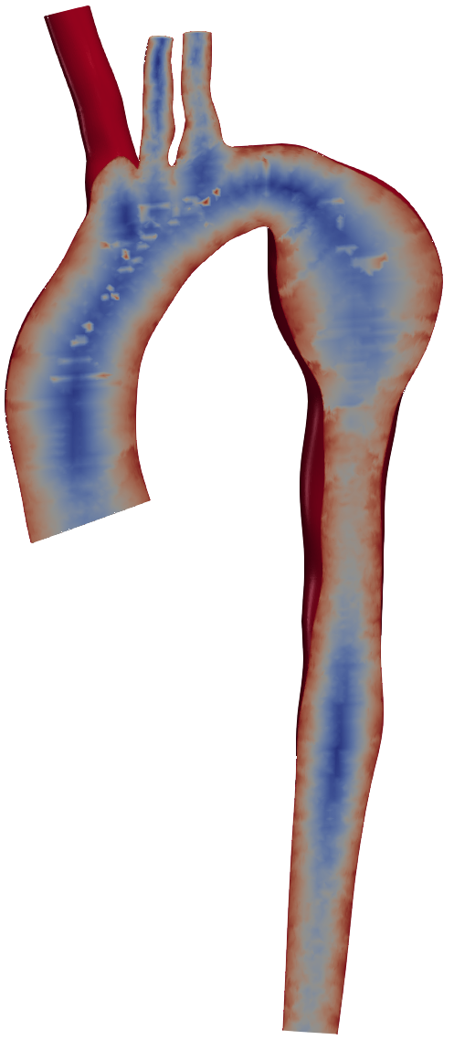
To map the 1D solution to the 3D Finite Element mesh, we create a map from nodes on the 1D centerline to nodes in the 3D volume mesh. This allows us to map quantities defined on the centerline to the volume mesh, such as 1D flow and pressure, cross-sectional area, and normal vectors. The iterative process is outlined in Algorithm 1 and visualized in Figure 2. In Line 1, we first create a set of seed points consisting of volume mesh nodes that are closest to the centerline nodes and store the corresponding indices in . To do this, we find the shortest Euclidean distances between centerline coordinates and 3D mesh coordinates . We then employ a region growing algorithm (Line 1) to grow the 1D-3D map outwards, starting from the centerline seed points . The algorithm in Line 1 selects nodes in the new layer from the previous layer using cell-connectivity. Finally, the map is expanded in Line 1 by assigning nodes in the new layer to the same 1D node as the closest 3D node in the previous layer . This results in centerline nodes being roughly assigned to 3D mesh nodes within the same cross-section. For 3D meshes with nodes Algorithm 1 only takes a few seconds to complete on a single CPU. We generate this map only once and use it repeatedly to map various centerline quantities to the volume mesh, see Figure 3.
2.6.3 Extrapolating pressure and velocity
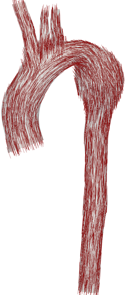
We directly map the pressure from the centerline to the volume mesh using the map generated in Section 2.6.2, resulting in a pressure that’s approximately constant over the cross-section of the vessels. However, as the 1D solution only provides a scalar flow along the centerline, we must generate a velocity vector field from scratch. The ingredients for the velocity vector field are visualized in Figure 3. From the mapped 1D flow rate and the cross-sectional area we calculate the velocity magnitude. Assuming a Poiseuille flow, we apply a parabolic flow profile to the velocity magnitude. With the help of a normalized radial coordinate, we prescribe the flow profile to be maximal on the centerline and zero on the boundary. Finally, we multiply the scalar velocity magnitude with the centerline tangent vector to generate a vector field. We aim to preserve the amount of flow through a cross-section of the vessel as obtained from the 1D solution while approximating a somewhat physiological velocity field. This velocity vector field can then be used for simulation initialization.
3 Results
Throughout this section, we consider a simulation periodically converged if the asymptotic error is , as defined in Equation (20). We utilize in this work a subset of 52 models from the Vascular Model Repository (vascularmodel.org) [35]. Six out of these models are shown in Table 1.
|
|
![[Uncaptioned image]](/html/2102.00107/assets/models/OSMSC0097_0001_sim.png)
|
![[Uncaptioned image]](/html/2102.00107/assets/models/OSMSC0107_0001_sim.png)
|
![[Uncaptioned image]](/html/2102.00107/assets/models/OSMSC0111_0001_sim.png)
|
![[Uncaptioned image]](/html/2102.00107/assets/models/OSMSC0130_0000_sim.png)
|
![[Uncaptioned image]](/html/2102.00107/assets/models/OSMSC0156_0001_sim.png)
|
|
| ID | 0003_0001 | 0097_0001 | 0107_0001 | 0111_0001 | 0130_0000 | 0156_0001 |
| Type | aorta-femoral | pulmonary | aorta | aorta | aorta | aorta-femoral |
| State | normal | Glenn | end-to-end anastomosis | coarctation | aneurysm | aneurysm |
3.1 Convergence
In this section, we detail the convergence behavior of cardiovascular fluid dynamics simulations with three-element Windkessel, or RCR, boundary conditions. The models used in this section have different numbers of outlets, ranging from 4 in the aortic models to 33 in the pulmonary artery models. For each model, we automatically generate a reduced-order 0D model as outlined in Section 2.3. Using a computationally inexpensive 0D model allows us to run a large number of simulations for many cardiac cycles and analyze their convergence behavior in detail. These 0D results are directly applicable to 1D and 3D simulation models and form the foundation for generating initial conditions in Section 3.2.2.
3.1.1 Time constants
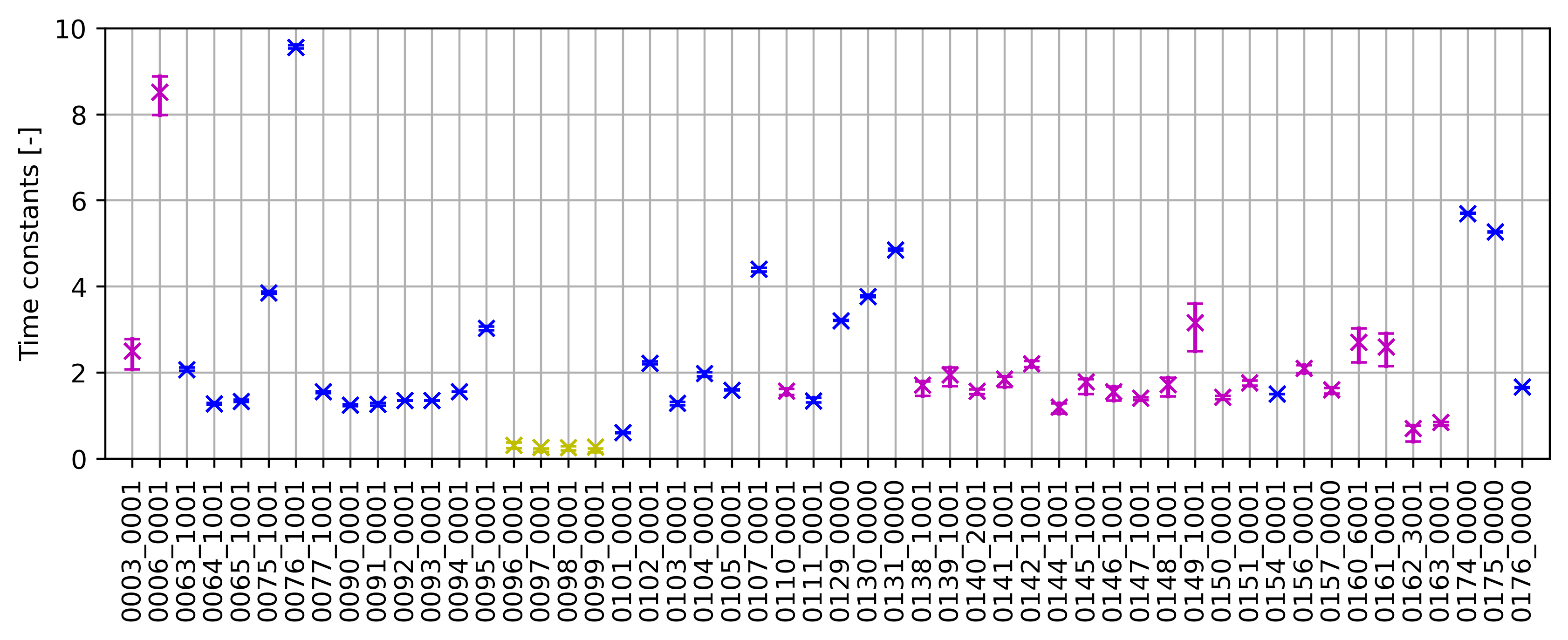
The time constant is the metric of a boundary condition that determines the rate of periodic convergence. It is thus essential for all numerical experiments in this work. Throughout the remainder of this work, we normalize by the length of the cardiac cycle , with all values reported in Figure 4. All normalized time constants fall within the range , with time constants in pulmonary models being the lowest. Furthermore, the time constants of different outlets in one model all fall within a narrow range. In addition to the outlet time constants, we also show the model time constants as crosses. We extract the model time constants from the slope of the exponential curves of the asymptotic error (see Equation (20)) when running the models for several cardiac cycles. Each model has one unique model time constant that is approximately the mean value of the outlet time constants.
3.1.2 Initial conditions
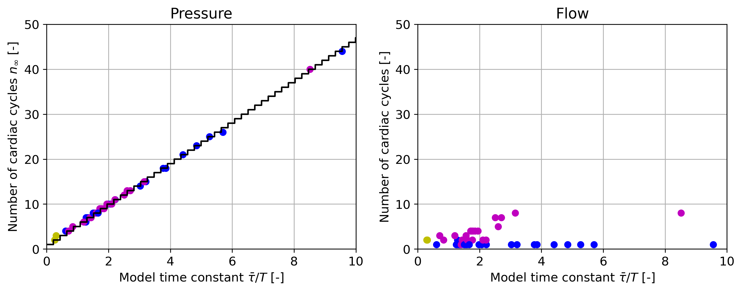
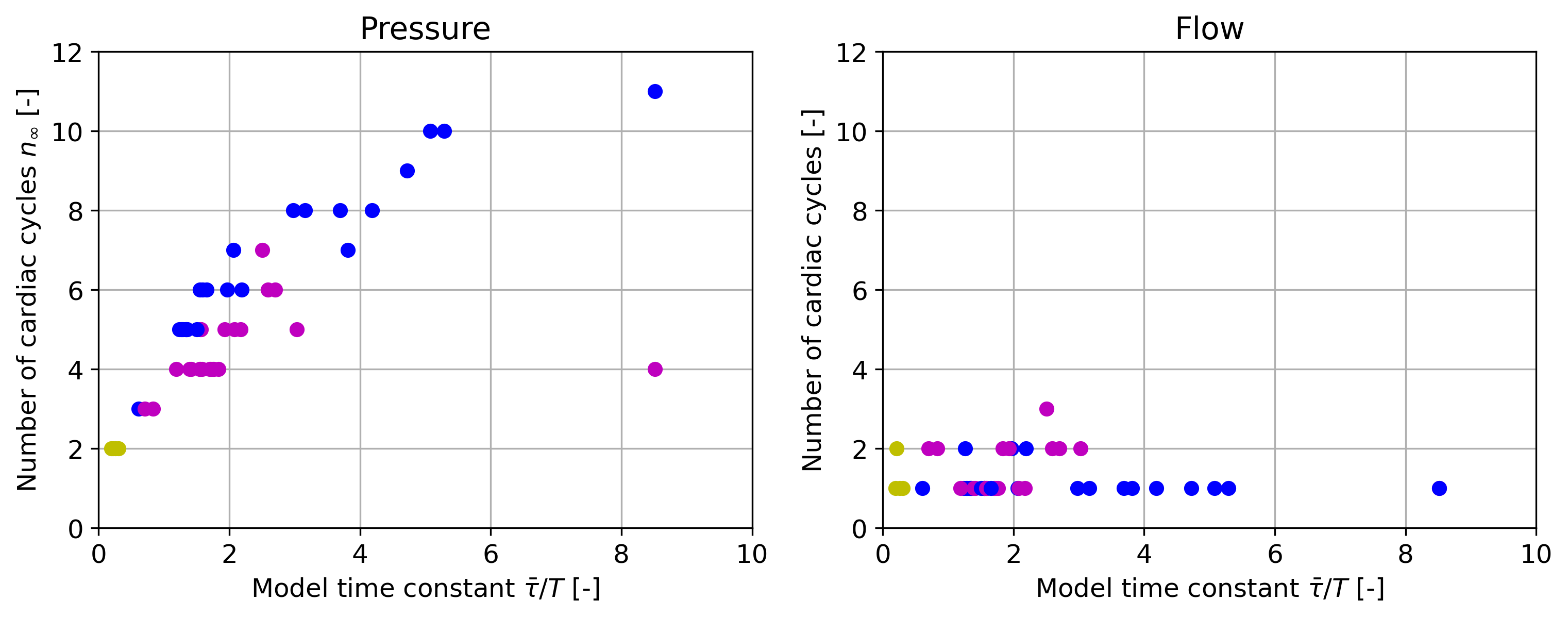
We estimated the number of cardiac cycles required to reach a periodic pressure in Equation (20). In the special case of zero initial conditions, this relationship simplified to the inequality in Equation (21), scaling linearly with the time constant and the logarithm of the asymptotic error . This relationship holds regardless of model fidelity, i.e. for 0D, 1D, and 3D. In Figure 5(a), we record the number of cardiac cycles required to reach an asymptotic error of when starting a simulation from zero initial conditions, and report the number of cardiac cycles required for periodic pressure (left) and flow (right) over the model time constant . For pressure (left), the results confirm the linear relationship between the single model time constant and the number of cardiac cycles from Equation (21) (black line). For a range of model time constants we find the range of cardiac cycles . The number of cardiac cycles to reach a periodic flow solution (right) is not correlated to the model time constant and is, in general, much lower than the number of cycles to reach a periodic pressure. Flow rate commonly converges within one cardiac cycle, with a maximum of eight cardiac cycles in our cohort of models.
The same study is repeated in Figure 5(b) for starting from steady state initial conditions. Compared to zero initial conditions, the number of cardiac cycles required to each an asymptotic pressure with an error of are much lower: . Flow is converged within a maximum of 5 cardiac cycles. When starting from steady state initial conditions, the number of cardiac cycles cannot be given analytically, it depends on the prescribed inflow profile. However, the number of cardiac cycles commonly still increases with the model time constant.
3.1.3 Comparison of error metrics
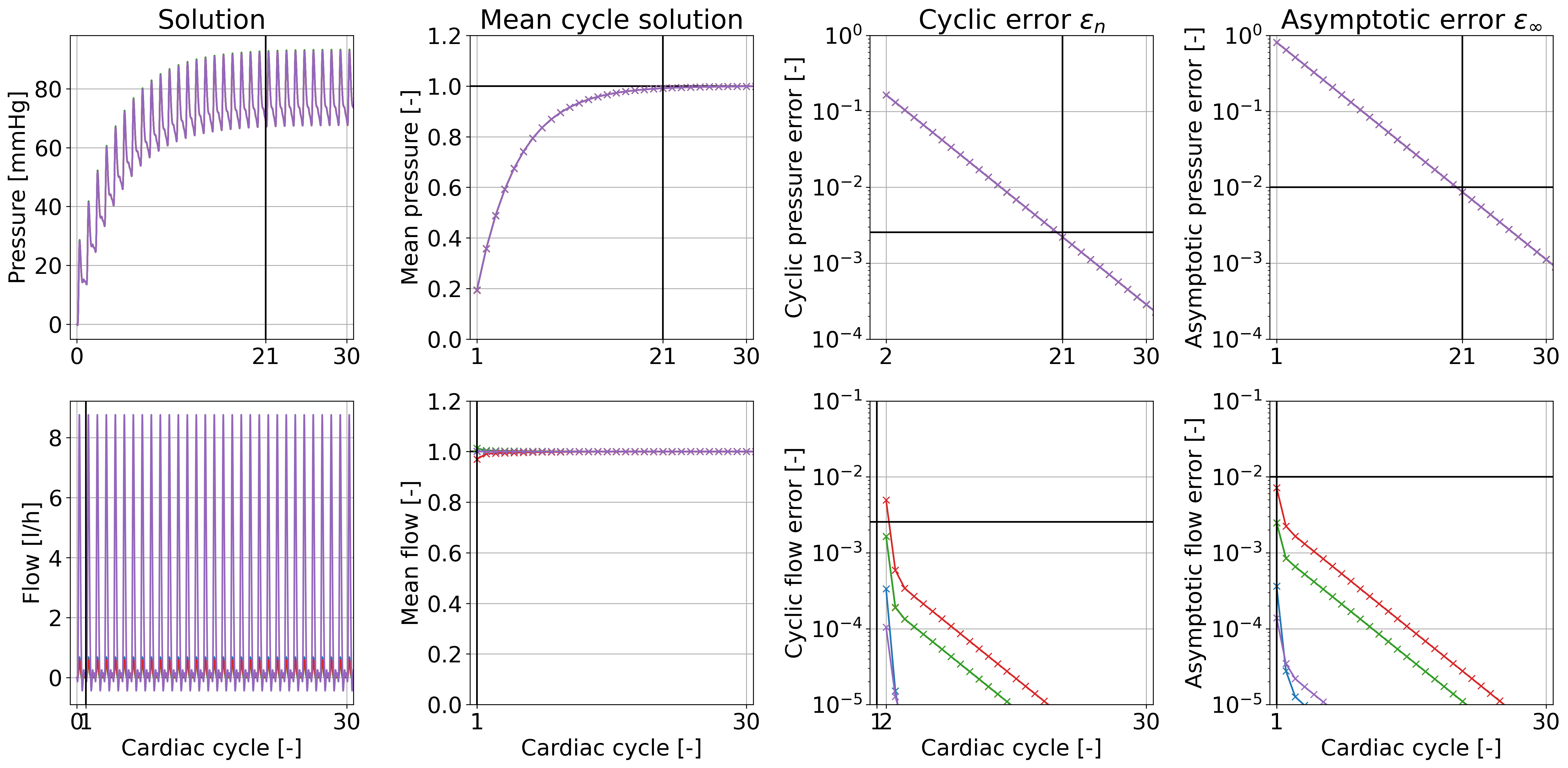
We visualize the convergence of pressure and flow for cardiac cycles in Figure 6 for model 0107_0001 (normal aorta). The pressure curve (top left) builds up slowly in each cardiac cycle, starting from zero, whereas the flow curve (bottom) is close to periodic starting from the first cycle. Taking the mean value over each cardiac cycle, both solutions exponentially approach their periodic state, as shown in Equation (18). The logarithmic plots in the two rightmost columns show the exponential decay of the cyclic error and the asymptotic error , as defined in Equations (20) and (22), respectively. Note that the flow (bottom) exhibits smaller errors than the pressure (top) and converges faster during the first few cardiac cycles. After that, both flow and pressure at all outlets converge with the model time constant . This model time constant yields a factor between cyclic and asymptotic error of . The threshold is indicated by horizontal lines in the error plots. Here, the solution is converged after cardiac cycles, reaching errors of and . This example demonstrates that for simulations with the cyclic error underestimates the asymptotic error .
3.1.4 Prediction of the periodic state
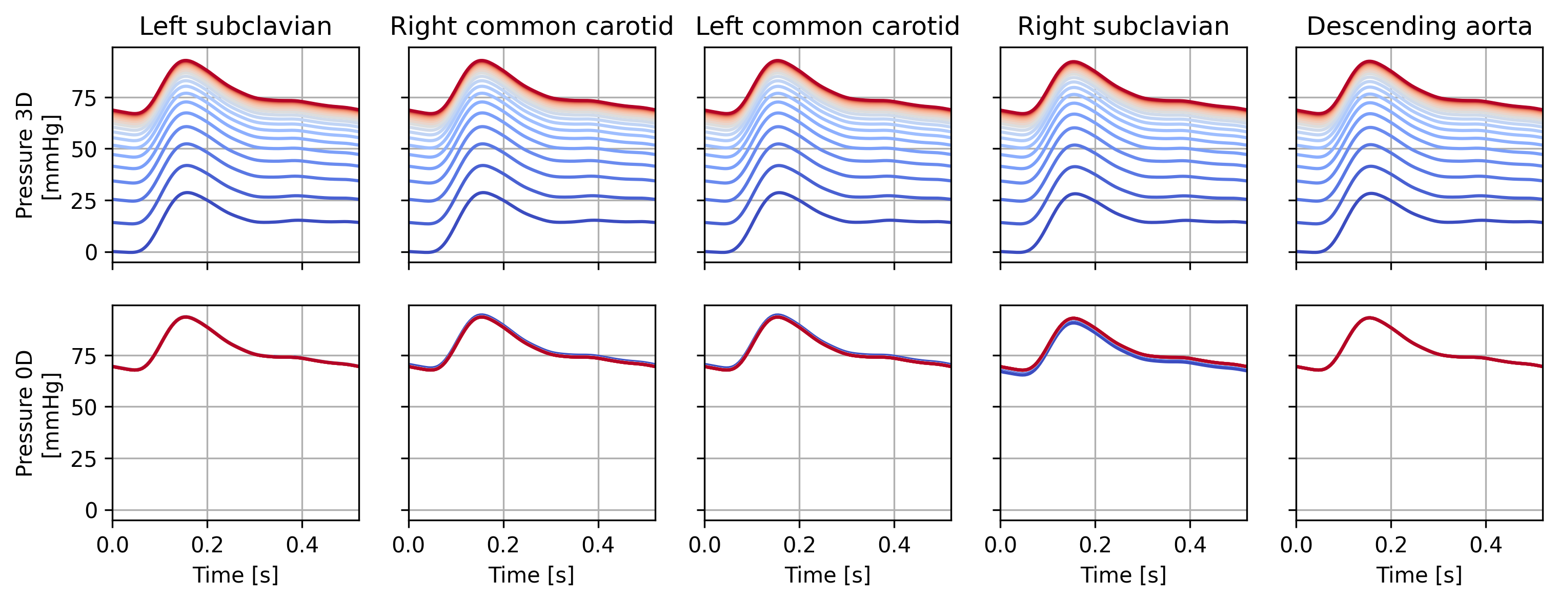
As explained in Section 2.4, the periodic error , comparing the current cardiac cycle to a perfectly periodic cycle, can in general not be computed analytically. It requires the periodic solution of the model which is not known a priori. We thus outlined a method in Section 2.5 to use the 0D lumped-parameter boundary condition to estimate the periodic cycle numerically. Figure 7 shows the pressure at all outlets of model 0107_0001 from cycle one to cycle (from blue to red), starting from zero initial conditions as in Figure 6. The top row shows the pressure at the outlets of the 3D model in each cardiac cycle. The bottom row shows the prediction of the periodic state using the flow at the outlets of the 3D model in each cardiac cycle. Since flow converges much faster than pressure in this model, see Figure 6, the cycle-to-cycle variation is minimal. The periodic state can be accurately predicted even from early cardiac cycles, where the actual pressure of the model has not yet converged.
3.2 Initialization
To demonstrate the performance of our 3D initialization method, we compare results for the 6 models shown in Table 1. The chosen models contain a wide range of anatomies and physiological conditions and are specified by an eight-digit ID. They include aorta and femoral arteries (0003_0001), pulmonary arteries after a Glenn procedure (0097_0001), aortic coarctation post end-to-end anastomosis (0107_0001), untreated aortic coarctation (0111_0001), aortic aneurysm in a patient with Marfan Syndrome (0130_0000), and abdominal aortic aneurysm (0156_0001).
3.2.1 Generating initial conditions
In this section, we demonstrate the performance of our pipeline to generate 3D initial conditions that greatly reduce the number of cardiac cycles, as proposed in Section 2.6. As a ground truth, i.e. the ideal initial condition, we use an asymptotic 3D solution extracted after reaching periodic convergence. Using this initial condition, the 3D simulation would reach periodic converge within one cardiac cycle. We compare this solution to initial conditions we generated from a periodic 1D solution, using the mapping technique from Section 2.6.2. By using initial conditions mapped from 1D to 3D, we introduce two kinds of errors. First, the 1D solution is computed on a highly simplified geometrical representation of the 3D geometry assuming a constant flow profile, see Section 2.2. Second, the mapping process tries to but cannot guarantee local preservation of the 1D solution characteristics, such as incompressibility.
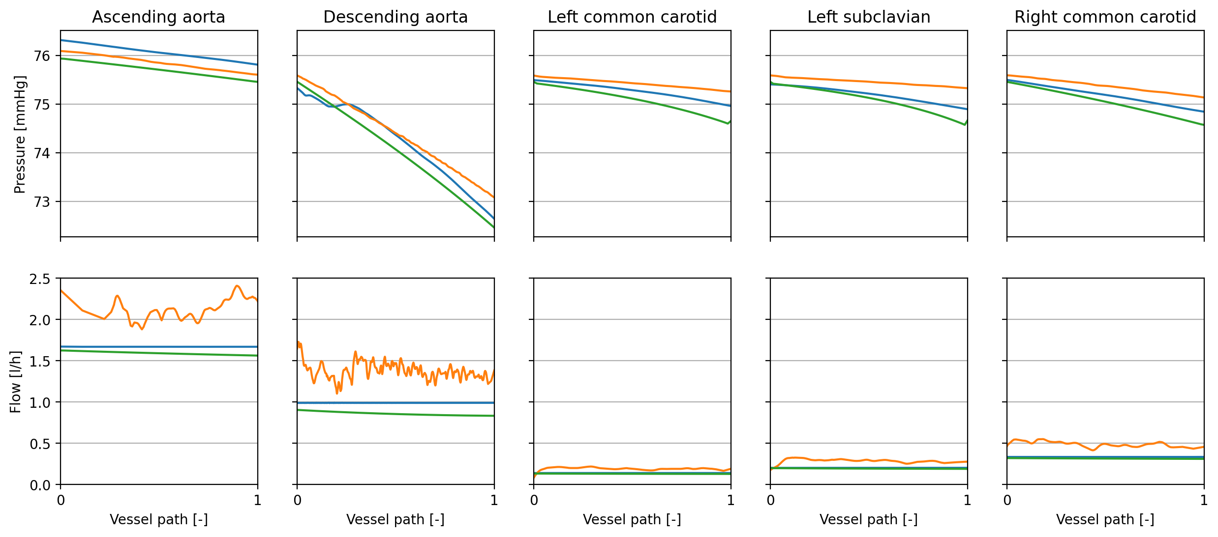
Figure 8 shows these errors by comparing different initial conditions: 3D ground truth (blue), 1D solution (green), and 3D mapped from 1D (orange). We integrate the 3D ground truth and the mapped 3D initial conditions over the cross-section of the 3D geometry continuously along the centerline. This allows us to plot pressure (top) and flow (bottom) continuously over the vessel path. For a perfect 1D approximation of the 3D simulation, the blue and green lines would overlap. For a perfect mapping from 1D to 3D, the blue and orange lines would overlap. In general, pressure is approximated well by the 1D model and mapped well to the 3D domain. The differences between the models ( mmHg) are small compared to the overall pressure level ( mmHg). Flow is approximated well by the 1D model whereas the the mapping results in oscillations and overestimates the actual flow. Since all three models should represent a model with rigid walls and incompressible flow, flow should be constant along the vessel path. However, the 3D mapped from 1D solution still roughly represents the correct flow splits to the different vessel branches.
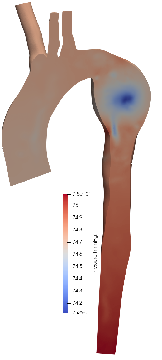
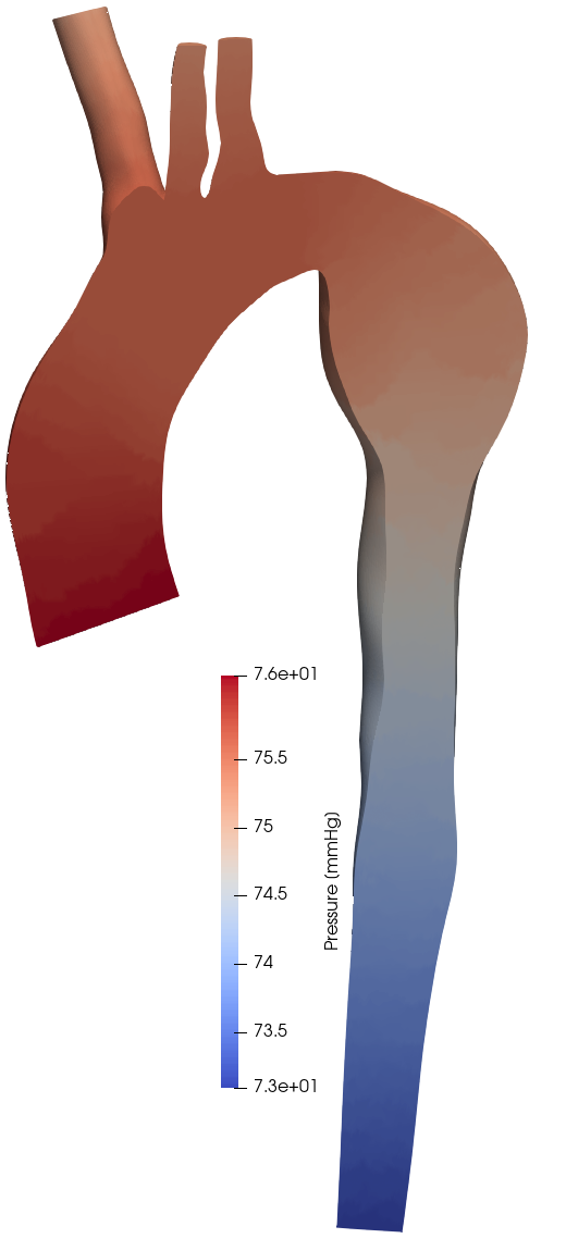
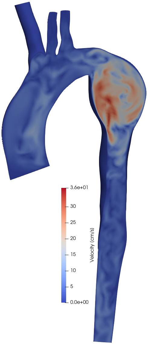
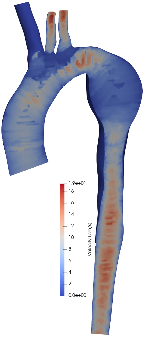
The differences between 3D ground truth and 3D mapped from 1D initial conditions are visualized in Figure 9(a) and are evident, especially within the aneurysm. The mapping from 1D to 3D results in a pressure that is approximately constant over the cross-sections of the vasculature. However, the overall variation, 74-75 mmHg in the ground truth and 73-76 mmHg in the extrapolated solution, is negligibly small compared to the overall pressure level. Similarly, the velocity field in Figure 9(b) is visibly different for the ground truth (left) and mapped solution (right).
3.2.2 Initial conditions
Finally, we demonstrate that 3D initial conditions mapped from periodic 1D solutions can greatly reduce the 3D simulation time. We compare three kinds of initial conditions: Zero, Steady, and 1D. For zero initial conditions, we prescribe uniformly and . To generate steady initial conditions, we first run a steady state simulation with constant mean inflow . We compared starting the pulsatile flow simulation at different time steps for model 0003_0001. Common choices are either the first time step or the time step where the inflow closely matches the mean flow [5]. We found that the number of cardiac cycles required to reach periodic convergence was not affected by the choice of starting time step, so for simplicity we chose for all comparisons in this section. For 1D initial conditions, we use the framework proposed in Section 2.6. The 3D simulations were run using an incompressible Newtonian fluid, a rigid wall, and a no-slip condition at the wall. All 1D simulations and the mapping from 1D to 3D were run a single CPU on a workstation computer.
Figure 10 shows the convergence of the asymptotic error for pressure (top) and flow (bottom) at all outlets (colors) for all three initial conditions: zero (left), steady (middle), 1D (right). The threshold is indicated by a horizontal line, the number of cardiac cycles required to reach that threshold is indicated in each simulation by a vertical line. All simulations are shown for a total of cardiac cycles. Note that the scale of the flow error is one magnitude lower than the scale of the pressure error. From left to right, the flow and pressure solutions start with a successively lower error in the first cardiac cycle. In the case of 1D initial conditions (right), the pressure errors of all outlets already fulfil the convergence criterion after only one cardiac cycle. Both pressure and flow errors stagnate below as other numerical errors in the simulations outweigh the asymptotic error. As previously observed, pressure converges faster than flow when using zero or steady initial conditions. However, pressure and flow are converged in one and two cardiac cycles, respectively, when using 1D initial conditions. Due to the drastic reduction in the number of cardiac cycles required for the pressure solution, flow is now slightly slower to converge.
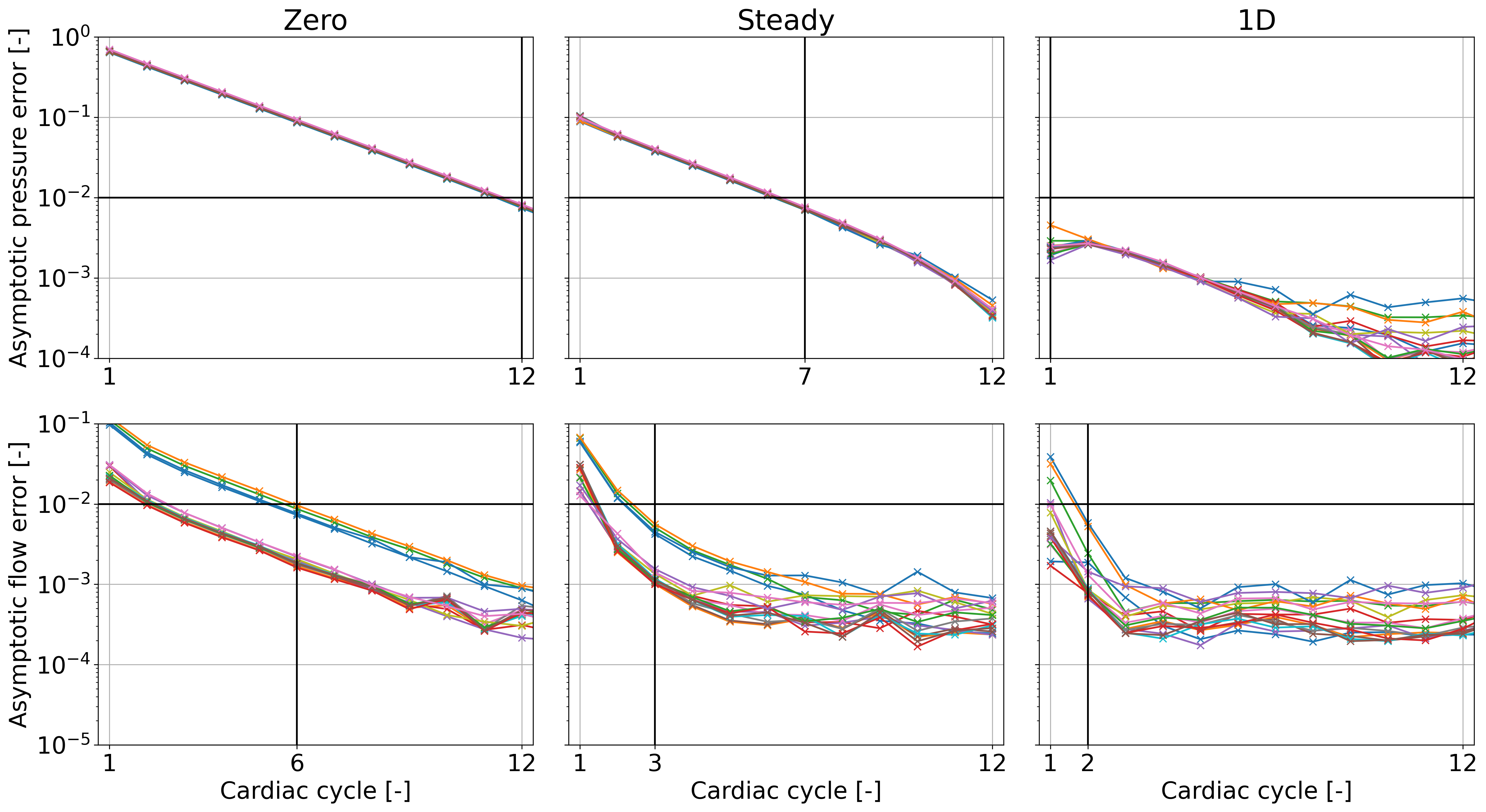
Convergence results for all selected 3D geometries and are reported in Table 2. While initializing with a steady state solution considerably reduces the number of cardiac cycles to reach convergence, most of the models still require at least five cardiac cycles for convergence. In all models, the simulations initialized with the 1D solution converge in one or two cardiac cycles. This leads to speedup factors between one and nine compared to the steady state initialization, saving between 0 and 53 h of computation time on 48 CPU cores each per 3D model. Only in model 0097_0001 which has a very low model time constant and the simulation even with zero initial conditions converges in two iterations does the 1D initialization not yield a speedup.
| ID | 0003_0001 | 0097_0001 | 0107_0001 | 0111_0001 | 0130_0000 | 0156_0001 |
| 2.2 h | 1.7 h | 1.9 h | 6.3 h | 6.6 h | 6.4 h | |
| 2.5 | 0.2 | 4.4 | 1.3 | 3.8 | 2.1 | |
| Zero | 12 / 6 | 2 / 2 | 20 / 1 | 7 / 1 | 16 / 1 | 10 / 3 |
| Steady | 7 / 3 | 2 / 2 | 6 / 1 | 5 / 2 | 9 / 3 | 5 / 2 |
| 1D | 1 / 2 | 1 / 2 | 1 / 1 | 1 / 1 | 1 / 1 | 1 / 2 |
| 11 h | 0 | 9.5 h | 25 h | 53 h | 19 h |
4 Discussion
We gave a detailed review of properties of lumped-parameter boundary conditions in cardiovascular fluid dynamics simulations. The speed of convergence to a periodic state solution is determined by a single model time constant, that can be approximated as the mean of all individual time constants of multiple outlet boundary conditions. We found that for 53 models of the Vascular Model Repository, the model time constant spanned from 0.3 in pulmonary models to 9.6 in aorta models. That means that in the most extreme case, the time constant of the model is almost ten times as large as the length of the cardiac cycle. Using zero initial conditions, the number of cardiac cycles required to reach a periodic state scales linearly with the model time constant, reaching a median of eight cardiac cycles for our subset of models. Even when using initial conditions other than zero, e.g., from a steady state solution, the number of cardiac cycles required still scales with model time constant.
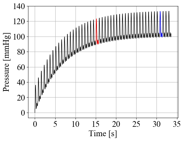
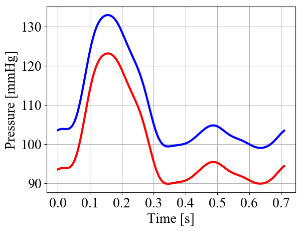
We introduced the asymptotic error to determine whether a simulation has reached a periodic state, calculating the relative difference of the results in the current cardiac cycle to a perfectly periodic solution. As the periodic solution is not known a priori, we proposed to use a 0D model of the boundary condition. Taking the flow at a 3D outlet as input, we estimate the periodic pressure and compare it to the pressure at the 3D outlet. This method is a quick and easy validation tool for any 3D vascular fluid dynamics simulation with lumped-parameter boundary conditions. In models with time constants larger than , the cycle-to-cycle difference is lower than the asymptotic error. A low cycle-to-cycle difference can erroneously lead the user to believe that the simulation has already reached a periodic state when comparing two consecutive cardiac cycles. This is visualized in Figure 11. Using the same error tolerance of 1 % but different error norms, cyclic error (red) and asymptotic error (blue), yields a pressure difference of 10 mmHg. Thus, only the asymptotic error is a suitable metric to determine the distance of a simulation to its periodic state.
To reduce 3D computation times, we proposed a method to generate good initial conditions in an automated and computationally inexpensive way. We used SimVascular to automatically generate a 1D replication of the 3D model, which we ran until we achieved a periodic state. We than mapped the 1D solution onto the 3D Finite Element mesh. Note that the mapping does in general not result in a fluid field that is divergence free. However, we are not interested in generating a physical or physiological meaningful solution. Instead, the initial conditions are “washed out” by the first iteration of our numerical solver of the Navier Stokes equations. Similarly, the pressure field does not capture local variations. Here, it should be noted that it is much more important to match the overall pressure level of the model, which is in general much higher than any local variations. In a convergence analysis with six different vascular models, we demonstrated that models with our 1D initialization method converge in one or two cardiac cycles. This greatly reduces the computation time for the 3D model over the standard method of initializing pulsatile simulations with a steady-state solution, typically dozens of hours in simulation time and hundreds of hours in CPU time. The code for the 1D initialization is freely available on GitHub (github.com/SimVascular/SimVascular).
We close with a discussion of the the limitations and future perspectives of our work. We did only consider RCR boundary conditions in this work. However, there are many more examples of lumped parameter 0D networks that are coupled to 3D models, such as coronary boundary conditions [36, 37] and 0D closed loop models used, e.g., in simulations for single ventricle [38, 39] and coronary artery bypass graft (CABG) patients [40]. In the general case of lumped parameter boundary conditions, the model time constant cannot be determined analytically. However, it can still be calculated numerically from the time it takes the boundary condition to respond to a step in the inflow condition. We plan to include these boundary conditions in future work. It should be noted that those boundary conditions not only require initialization of the velocity and pressure field in the 3D model but also in unknowns that are internal to the 0D model. Furthermore, we only considered rigid-wall simulation in this work. We plan to test our 1D initialization method for deformable wall simulations as well, using the coupled momentum method [41] or an arbitrary Lagrangian–Eulerian formulation [42]. To further improve our method and guarantee periodic convergence within one cardiac cycle, it will be necessary to improve the mapping of the velocity field to the 3D model. This could be accomplished for example by solving a Stokes flow problem, using the 1D results as boundary conditions.
5 Acknowledgments
We thank Dr. Luca Pegolotti and Dr. Irene Vignon-Clementel for insightful discussions. This work was supported by NIH grants R01LM013120 and R01EB029362. The authors gratefully acknowledge the Stanford Research Computing Center for providing the computational resources necessary to the numerical simulations presented in this work.
References
- [1] Ethan Kung, Alessia Baretta, Catriona Baker, Gregory Arbia, Giovanni Biglino, Chiara Corsini, Silvia Schievano, Irene E. Vignon-Clementel, Gabriele Dubini, Giancarlo Pennati, Andrew Taylor, Adam Dorfman, Anthony M. Hlavacek, Alison L. Marsden, Tain-Yen Hsia, and Francesco Migliavacca. Predictive modeling of the virtual hemi-fontan operation for second stage single ventricle palliation: Two patient-specific cases. Journal of Biomechanics, 46(2):423–429, jan 2013.
- [2] Jongmin Seo, Casey Fleeter, Andrew M. Kahn, Alison L. Marsden, and Daniele E. Schiavazzi. Multi-fidelity estimators for coronary circulation models under clinically-informed data uncertainty. arXiv, 2019.
- [3] Casey M. Fleeter, Gianluca Geraci, Daniele E. Schiavazzi, Andrew M. Kahn, and Alison L. Marsden. Multilevel and multifidelity uncertainty quantification for cardiovascular hemodynamics. Computer Methods in Applied Mechanics and Engineering, 365:113030, jun 2020.
- [4] Christopher J. Arthurs, Nan Xiao, Philippe Moireau, Tobias Schaeffter, and C. Alberto Figueroa. A flexible framework for sequential estimation of model parameters in computational hemodynamics. Advanced Modeling and Simulation in Engineering Sciences, 7(1), dec 2020.
- [5] I.E. Vignon-Clementel, C.A. Figueroa, K.E. Jansen, and C.A. Taylor. Outflow boundary conditions for 3d simulations of non-periodic blood flow and pressure fields in deformable arteries. Computer Methods in Biomechanics and Biomedical Engineering, 13(5):625–640, oct 2010.
- [6] Jing Wan, Brooke Steele, Sean A. Spicer, Sven Strohband, Gonzalo R. Feijo´o, Thomas J.R. Hughes, and Charles A. Taylor. A one-dimensional finite element method for simulation-based medical planning for cardiovascular disease. Computer Methods in Biomechanics and Biomedical Engineering, 5(3):195–206, jan 2002.
- [7] S. M. Moore, K. T. Moorhead, J. G. Chase, T. David, and J. Fink. One-dimensional and three-dimensional models of cerebrovascular flow. Journal of Biomechanical Engineering, 127(3):440–449, sep 2004.
- [8] L. Grinberg, E. Cheever, T. Anor, J. R. Madsen, and G. E. Karniadakis. Modeling blood flow circulation in intracranial arterial networks: A comparative 3d/1d simulation study. Annals of Biomedical Engineering, 39(1):297–309, jul 2010.
- [9] Philippe Reymond, Fabienne Perren, François Lazeyras, and Nikos Stergiopulos. Patient-specific mean pressure drop in the systemic arterial tree, a comparison between 1-d and 3-d models. Journal of Biomechanics, 45(15):2499–2505, oct 2012.
- [10] Nan Xiao, Jordi Alastruey, and C. Alberto Figueroa. A systematic comparison between 1-d and 3-d hemodynamics in compliant arterial models. International Journal for Numerical Methods in Biomedical Engineering, 30(2):204–231, sep 2013.
- [11] S. Pant, B. Fabrèges, J-F. Gerbeau, and I. E. Vignon-Clementel. A methodological paradigm for patient-specific multi-scale CFD simulations: from clinical measurements to parameter estimates for individual analysis. International Journal for Numerical Methods in Biomedical Engineering, 30(12):1614–1648, nov 2014.
- [12] Giulia Bertaglia, Adrián Navas-Montilla, Alessandro Valiani, Manuel Ignacio Monge García, Javier Murillo, and Valerio Caleffi. Computational hemodynamics in arteries with the one-dimensional augmented fluid-structure interaction system: viscoelastic parameters estimation and comparison with in-vivo data. Journal of Biomechanics, 100:109595, feb 2020.
- [13] Adam Updegrove, Nathan M. Wilson, Jameson Merkow, Hongzhi Lan, Alison L. Marsden, and Shawn C. Shadden. SimVascular: An open source pipeline for cardiovascular simulation. Annals of Biomedical Engineering, 45(3):525–541, dec 2016.
- [14] Leopoldo P. Franca and Sérgio L. Frey. Stabilized finite element methods: II. the incompressible navier-stokes equations. Computer Methods in Applied Mechanics and Engineering, 99(2-3):209–233, sep 1992.
- [15] Charles A. Taylor, Thomas J.R. Hughes, and Christopher K. Zarins. Finite element modeling of blood flow in arteries. Computer Methods in Applied Mechanics and Engineering, 158(1-2):155–196, may 1998.
- [16] Christian H. Whiting and Kenneth E. Jansen. A stabilized finite element method for the incompressible navier-stokes equations using a hierarchical basis. International Journal for Numerical Methods in Fluids, 35(1):93–116, 2001.
- [17] Mahdi Esmaily-Moghadam, Yuri Bazilevs, and Alison L. Marsden. A new preconditioning technique for implicitly coupled multidomain simulations with applications to hemodynamics. Computational Mechanics, 52(5):1141–1152, may 2013.
- [18] Thomas J.R. Hughes and J. Lubliner. On the one-dimensional theory of blood flow in the larger vessels. Mathematical Biosciences, 18(1-2):161–170, oct 1973.
- [19] B.N. Steele, Jing Wan, J.P. Ku, T.J.R. Hughes, and C.A. Taylor. In vivo validation of a one-dimensional finite-element method for predicting blood flow in cardiovascular bypass grafts. IEEE Transactions on Biomedical Engineering, 50(6):649–656, jun 2003.
- [20] Mette S. Olufsen. Structured tree outflow condition for blood flow in larger systemic arteries. American Journal of Physiology-Heart and Circulatory Physiology, 276(1):H257–H268, jan 1999.
- [21] Luca Antiga, Marina Piccinelli, Lorenzo Botti, Bogdan Ene-Iordache, Andrea Remuzzi, and David A. Steinman. An image-based modeling framework for patient-specific computational hemodynamics. Medical & Biological Engineering & Computing, 46(11):1097–1112, nov 2008.
- [22] Alexander N. Brooks and Thomas J.R. Hughes. Streamline upwind/petrov-galerkin formulations for convection dominated flows with particular emphasis on the incompressible navier-stokes equations. Computer Methods in Applied Mechanics and Engineering, 32(1-3):199–259, sep 1982.
- [23] Thomas J.R. Hughes and Michel Mallet. A new finite element formulation for computational fluid dynamics: III. the generalized streamline operator for multidimensional advective-diffusive systems. Computer Methods in Applied Mechanics and Engineering, 58(3):305–328, nov 1986.
- [24] Thomas J.R. Hughes, Leopoldo P. Franca, and Gregory M. Hulbert. A new finite element formulation for computational fluid dynamics: VIII. the galerkin/least-squares method for advective-diffusive equations. Computer Methods in Applied Mechanics and Engineering, 73(2):173–189, may 1989.
- [25] Mehran Mirramezani and Shawn C. Shadden. A distributed lumped parameter model of blood flow. Annals of Biomedical Engineering, jul 2020.
- [26] Luca Formaggia, Alfio Quarteroni, and Alessandro Veneziani, editors. Cardiovascular Mathematics. Springer Milan, 2009.
- [27] H. J. Kim, I. E. Vignon-Clementel, C. A. Figueroa, J. F. LaDisa, K. E. Jansen, J. A. Feinstein, and C. A. Taylor. On coupling a lumped parameter heart model and a three-dimensional finite element aorta model. Annals of Biomedical Engineering, 37(11):2153–2169, jul 2009.
- [28] Daniele E. Schiavazzi, Alessia Baretta, Giancarlo Pennati, Tain-Yen Hsia, and Alison L. Marsden. Patient-specific parameter estimation in single-ventricle lumped circulation models under uncertainty. International Journal for Numerical Methods in Biomedical Engineering, 33(3):e02799, jun 2016.
- [29] Irene E. Vignon and Charles A. Taylor. Outflow boundary conditions for one-dimensional finite element modeling of blood flow and pressure waves in arteries. Wave Motion, 39(4):361–374, apr 2004.
- [30] Mehran Mirramezani, Scott L. Diamond, Harold I. Litt, and Shawn C. Shadden. Reduced order models for transstenotic pressure drop in the coronary arteries. Journal of Biomechanical Engineering, 141(3), jan 2019.
- [31] Irene E. Vignon-Clementel, C. Alberto Figueroa, Kenneth E. Jansen, and Charles A. Taylor. Outflow boundary conditions for three-dimensional finite element modeling of blood flow and pressure in arteries. Computer Methods in Applied Mechanics and Engineering, 195(29-32):3776–3796, jun 2006.
- [32] Kenneth E. Jansen, Christian H. Whiting, and Gregory M. Hulbert. A generalized-alpha method for integrating the filtered navier–stokes equations with a stabilized finite element method. Computer Methods in Applied Mechanics and Engineering, 190(3-4):305–319, oct 2000.
- [33] Ryan L. Spilker and Charles A. Taylor. Tuning multidomain hemodynamic simulations to match physiological measurements. Annals of Biomedical Engineering, 38(8):2635–2648, mar 2010.
- [34] Yifang Zhou, Ghassan S Kassab, and Sabee Molloi. On the design of the coronary arterial tree: a generalization of murray's law. Physics in Medicine and Biology, 44(12):2929–2945, nov 1999.
- [35] Nathan M. Wilson, Ana K. Ortiz, and Allison B. Johnson. The vascular model repository: A public resource of medical imaging data and blood flow simulation results. Journal of Medical Devices, 7(4), dec 2013.
- [36] H.J. Kim, I.E. Vignon-Clementel, C.A. Figueroa, K.E. Jansen, and C.A. Taylor. Developing computational methods for three-dimensional finite element simulations of coronary blood flow. Finite Elements in Analysis and Design, 46(6):514–525, jun 2010.
- [37] H. J. Kim, I. E. Vignon-Clementel, J. S. Coogan, C. A. Figueroa, K. E. Jansen, and C. A. Taylor. Patient-specific modeling of blood flow and pressure in human coronary arteries. Annals of Biomedical Engineering, 38(10):3195–3209, jun 2010.
- [38] E. L. Bove, M. R. de Leval, F. Migliavacca, R. Balossino, and G. Dubini. Toward optimal hemodynamics: Computer modeling of the fontan circuit. Pediatric Cardiology, 28(6):477–481, aug 2007.
- [39] Edward L. Bove, Francesco Migliavacca, Marc R. de Leval, Rossella Balossino, Giancarlo Pennati, Thomas R. Lloyd, Sachin Khambadkone, Tain-Yen Hsia, and Gabriele Dubini. Use of mathematic modeling to compare and predict hemodynamic effects of the modified blalock–taussig and right ventricle–pulmonary artery shunts for hypoplastic left heart syndrome. The Journal of Thoracic and Cardiovascular Surgery, 136(2):312–320.e2, aug 2008.
- [40] Abhay B. Ramachandra, Andrew M. Kahn, and Alison L. Marsden. Patient-specific simulations reveal significant differences in mechanical stimuli in venous and arterial coronary grafts. Journal of Cardiovascular Translational Research, 9(4):279–290, jul 2016.
- [41] C. Alberto Figueroa, Irene E. Vignon-Clementel, Kenneth E. Jansen, Thomas J.R. Hughes, and Charles A. Taylor. A coupled momentum method for modeling blood flow in three-dimensional deformable arteries. Computer Methods in Applied Mechanics and Engineering, 195(41-43):5685–5706, aug 2006.
- [42] Kathrin Bäumler, Vijay Vedula, Anna M. Sailer, Jongmin Seo, Peter Chiu, Gabriel Mistelbauer, Frandics P. Chan, Michael P. Fischbein, Alison L. Marsden, and Dominik Fleischmann. Fluid–structure interaction simulations of patient-specific aortic dissection. Biomechanics and Modeling in Mechanobiology, 19(5):1607–1628, jan 2020.