The Galactic Chemical Evolution of Chlorine

Abstract

We measured ³⁵Cl abundances in 52 M giants with metallicities between –0.5 $<$ [Fe/H] $<$ 0.12. Abundances and atmospheric parameters were derived using infrared spectra from CSHELL on the IRTF and from optical echelle spectra. We measured Cl abundances by fitting a H³⁵Cl molecular feature at 3.6985 $\mu$m with synthetic spectra. We also measured the abundances of O, Ca, Ti, and Fe using atomic absorption lines. We find that the [Cl/Fe] ratio for our stars agrees with chemical evolution models of Cl and the [Cl/Ca] ratio is broadly consistent with the solar ratio over our metallicity range. Both indicate that Cl is primarily made in core-collapse supernovae with some contributions from Type Ia SN. We suggest other potential nucleosynthesis processes, such as the $\nu$-process, are not significant producers of Cl. Finally, we also find our Cl abundances are consistent with H II and planetary nebular abundances at a given oxygen abundance, although there is scatter in the data.

1 Introduction

The odd-Z element chlorine has few chemical abundance measurements in stars, yet is an intriguing element due to the multiple possible ways both stable isotopes of Cl, ³⁵Cl and ³⁷Cl, are thought to be produced. Stellar chlorine abundances are difficult to measure since no detectable optical or infrared atomic Cl lines have been found in FGK stars. Instead, HCl molecular lines have been used to measure Cl abundances. Due to the low Cl abundance relative to the even-Z elements and low dissociation energy of the HCl molecular (Martin $\&$ Hepburn, 1998), only the coolest stars have detectable HCl absorption lines. For example, ³⁵Cl abundances have been measured in the sun via sunspot umbrae spectra (Hall & Noyes, 1972) and in 16 M stars (Maas et al., 2016).

The Cl isotope ratio may be measured in molecular clouds using Cl bearing molecules and Cl nebular abundances are measured from forbidden Cl transitions in planetary nebulae and H II regions. H II region abundances have compared Cl to O and found the [Cl/O] ratio is nearly constant with galactocentric radius and therefore both elements evolve in lockstep (Esteban et al., 2015; Arellano-Córdova et al., 2020). H II regions in M31 also show a relationship between Cl and O with more scatter (Fang et al., 2018). Similar Cl to O correlations have been found in planetary nebulae in the Galaxy (Henry et al., 2004; Milingo et al., 2010) and abundances have shown that Cl evolves in lockstep with Ar (Delgado-Inglada et al., 2015).

The Cl isotope ratio has varies both in the interstellar medium (ISM) and in a small sample of measured M giants. ³⁵Cl and ³⁷Cl bearing molecules have been measured in the circumstellar envelopes of evolved stars such as IRC+10216 (Cernicharo et al., 2000; Kahane et al., 2000; Highberger et al., 2003), in molecular gas in star formation regions such as the Orion Nebula (Salez et al., 1996; Cernicharo et al., 2010; Peng et al., 2010; Neufeld et al., 2012, 2015; Kama et al., 2015), towards bright infrared sources, and in intergalactic sources, along sight-lines toward quasars (Muller et al., 2014; Wallström et al., 2019). Combining the results from all the surveys reveals a large range in Cl isotope ratios from 1 $<$ ³⁵Cl/³⁷Cl $<$ 5 in the ISM. A scatter of 1.76 $<$ ³⁵Cl/³⁷Cl $<$ 3.42 was also measured in a small sample of six M giants (Maas & Pilachowski, 2018). The origin of the Cl isotope ratio scatter is still unknown but may be due to differences in local enrichment or self-enrichment. For example, the s-process may lower the Cl isotope ratio when compared to the solar value (Highberger et al., 2003; Cristallo et al., 2015; Karakas & Lugaro, 2016).

Both Cl isotopes are predicted to be produced in core collapse supernovae (CCSNe) during explosive oxygen with ³⁵Cl produced from proton capture on sulfur and ³⁷Cl from the radioactive decay of ³⁷Ar (Woosley et al., 1973; Thielemann & Arnett, 1985; Woosley & Weaver, 1995). Both isotopes may be produced in Type Ia supernovae, however the contribution is not thought to be as significant as CCSNe (Travaglio et al., 2004; Leung & Nomoto, 2018). The weak s-process in massive stars is thought to be a significant source of ³⁷Cl (Prantzos et al., 1990; Pignatari et al., 2010) while the s-process in AGB stars is not thought to be as important (Cristallo et al., 2015; Karakas & Lugaro, 2016). ³⁵Cl may also be produced from neutrino spallation during CCSNe (Woosley et al., 1990). Finally, the interaction and merger of the carbon and oxygen burning shells in massive stars may increase the production of the odd-Z light elements, including Cl (Ritter et al., 2018). A summary of the yields from the different proposed nucleosynthesis sites of Cl are listed in Table 1 of Maas & Pilachowski (2018).

Chemical evolution models predict the Cl to iron ratio will be nearly constant between –0.16 $\lesssim$ [Cl/Fe] $\lesssim$ –0.26 over –4 $<$ [Fe/H] $<$ 0.2 (Kobayashi et al., 2011; Prantzos et al., 2018). Contributions from rotating massive stars are important at low [Fe/H] although less significant between –1 $<$ [Fe/H] $<$ 0.2 (Prantzos et al., 2018). Other chemical evolution models suggest a more complex evolution of Cl, with [Cl/Fe] $\sim$ –0.8 at [Fe/H] = –2 (Kobayashi et al., 2020). A sample of 16 stars with Cl abundances between –0.72 $<$ [Fe/H] $<$ 0.2 was broadly consistent with chemical evolution models and possibly models under-predicted the measurements (Maas et al., 2016). However, the sample size was small and the typical uncertainties were 0.23 dex.

To understand the production sites and Galactic chemical evolution of chlorine, we have measured Cl abundances in 52 M giant stars, as discussed in Maas (2020). Section 2 describes the observations and data reduction. Section 3 details the atmospheric parameter ($T_{\mathrm{eff}}$, log(g), [Fe/H], microturbulence) derivations. Elemental abundance and uncertainty measurements are characterized in section 4. The results are discussed in section 5 and the conclusions summarized in section 6.

2 Observations and Data Reduction

2.1 Sample Selection

We chose sample stars first based on their effective temperature and their observed K_s magnitude. The HCl molecule has a low dissociation energy (Martin $\&$ Hepburn, 1998) and therefore only low temperature stars are able to form detectable HCl ro-vibrational features. Maas et al. (2016) examined stars from a range of $T_{\mathrm{eff}}$ from 3300 K to 4300 K and found only stars with $T_{\mathrm{eff}}$ $\lesssim$ 4000 K had detectable H³⁵Cl features. The sky background is also significant at 3.7 $\mu$m, the approximate location of the targeted HCl molecular features, and can dominate the observed signal for long exposure times. Therefore, to achieve the signal-to-noise ratios necessary (S/N $>$ 100 from Maas et al. 2016), stars with K_s $<$ 4 mag were chosen for observations using DIRBE (Hauser et al., 1998; Smith et al., 2004) and 2MASS photometry (Skrutskie et al., 2006).

We also derived thin and thick disk membership probabilities for the stars meeting both criteria listed above. The population membership probabilities were derived using U V W Galactic velocity components from Famaey et al. (2005) and equations 1 and 2 from Ramírez et al. (2013). Both thin and thick disk stars were selected to explore the abundance pattern of the disk. Finally, binaries and variable stars were removed from the sample using the SIMBAD database.

Few M giants in the sample had previously determined atmospheric parameters in the literature. Optical echelle spectra for each target star was obtained, along with IR spectra, in order to determine [Fe/H] abundances, microturbulence values, and abundances of additional elements. We obtained high resolution spectra for 52 stars in total; a list of the final sample is given in Table 1.

Table 1: Sample and Observation Summary

HD	Ks	Ks	S/N	Echelle	S/N
Num.	(Mag.)	Source	(IR)	Source	(Optical)
5111	2.8	1	70	1	40
15594	1.3	1	100	1	120
19258	2.14	2	150	1	60
25000	1.53	2	130	1	90
30634	2.35	2	200	1	60
31072	3.05	2	130	1	60
35067	3.08	2	50	1	50
84181	3.0	1	150	1	90
99592	0.52	2	180	1	100
102159	0.78	2	160	2	20
103340	3.9	1	40	1	50
108815	1.87	2	200	1	80
114941	3.54	2	110	1	80
115322	1.36	2	150	1	110

Note. — K_s Sources: (1) 2MASS (Skrutskie et al., 2006), (2) DIRBE (Hauser et al., 1998; Smith et al., 2004)

Note. — Echelle Spectra Sources: (1) ARCES on APO 3.5m, (2) TOU on 50” Dharma Endowment Foundation Telescope

Note. — (This table is available in its entirety in machine-readable form.)

2.2 IRTF Observations and IR Spectra Data Reduction

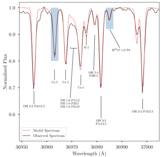
Our target stars were observed with CSHELL (Tokunaga et al., 1990; Greene et al., 1993) on the 3m NASA Infrared Telescope Facility (IRTF). The central wavelength for observations was 36980 Å to best observe the H³⁵Cl feature at 36985.1 Å and the total wavelength range is $\sim$ 70 Å. A slit width of 0.5” was chosen to achieve a resolution of R $\sim$ 40,000, necessary to resolve the H³⁵Cl feature from a nearby OH line.

Data reduction was performed with PyRAF following standard infrared spectroscopic data reduction procedures (Joyce, 1992). First, the raw observations were trimmed, flatfielded, and dark subtracted using median combined calibration images. Targets were nodded along the slit and pairs of images were taken in two different spatial positions. We then subtracted the nodded pair of images from one another to remove the bias and sky background. Spectra were then extracted from each observation. A wavelength solution derived from atomic Ca I and OH lines were applied to the data using the linelist in Maas et al. (2016). The spectral range contains too few telluric features for an independent wavelength solution. Signal-to-noise calculations are given in Table 1 and were estimated by calculating the standard deviation on observed data from the normalized continuum in regions with no stellar absorption features. The specific regions used are between 36948 Å - 36952 Å, 36958 Å - 36961.1 Å, and from 37013 Å - 37019 Å.

After the wavelength solution was calculated for extracted stellar spectra, they were median combined. Any observations with apertures near the edge of the detector when nodded were not used in the final combination to ensure only accurately traced images were included. After the wavelength solution was applied, telluric lines were divided out of the object spectrum using observations of spectral type A and B telluric standard stars. The airmass difference between the telluric standard and object was limited to 0.1 and the airmass was $\leq$ 1.1 for most observations. 52 stars in total were observed using CSHELL in 2016A and 2016B. The final spectra were normalized and we achieved S/N ratios above 100 for most targets with individual S/N ratios listed in Table 1.

Figure 1: An example CSHELL spectrum of the star HD 123303. The black line is the observation while the red line is a model spectrum. Important atomic and molecular lines are identified. The blue shaded region represents the two lines used for abundance analysis and the wavelengths where the $\chi^{2}$ minimization was performed (see section 4.1).

2.3 Optical Spectra Observations and Data Reduction

The optical echelle spectra were obtained from two different facilities. First, we used ARCES (Wang et al., 2003) on the 3.5m Astrophysical Research Consortium (ARC) telescope at the Apache Point Observatory (APO). ARCES covers a spectral range between 3600 Å - 10000 Å with an approximate resolution of R $\sim$ 30,000. ARCES data were collected primarily for fainter objects ( V $\gtrsim$ 7 mag). The brighter targets in our sample were observed with TOU on the Dharma 50” Telescope (Ge et al., 2016). TOU covers a similar spectra range between 3800 Å - 9000 Å with a higher spectral resolution at R $\sim$ 100000. The source of each target’s optical spectrum observation is listed in Table 1.

The data reduction for observations taken at both observatories was completed using IRAF. The echelle data reduction followed standard steps and we followed the ARCES data reduction guide for data acquired at the ARC 3.5m telescope. During observations, bias, dome flats, and comparison ThAr spectra were observed each night. Blue and red flat field images were observed at both observatories. Cosmic rays were removed from the echelle spectra using the task cosmicrays and median combined bias images were used to subtract the bias level off all other images. Apertures were defined using the flatfield images and were extracted using apall. Next the object images were extracted and inter-order scattered light was removed using the task apscatter. The extracted object spectra were then flatfielded. ThAr reference spectra were used as the wavelength solution and chebyshev polynomials were used to fit the two dimensional wavelength solution in each image. The typical RMS uncertainty of the wavelength solution fit to the ThAr lamp lines was $\sim$ 0.005 Å for ARCES data and $\sim$ 0.003 Å for TOU data. Orders used for abundance analysis were normalize individually using the continuum task. The final signal-to-noise ratios are given in Table 1 and calculated in a similar way to the IR data although the regions without stellar absorption features were extremely limited. The regions of 7379.79 Å - 7380.535 Å, 7458.7 Å - 7458.82 Å, and 7534.6 Å - 7537.28 Å were used in the signal-to-noise ratio determinations.

3 Atmospheric Parameter Determination

Typically, atmospheric parameters are derived using Fe I and Fe II excitation and ionization balance. However, the spectral range of our CSHELL spectra is very limited and few Fe II lines exist in the M giant optical spectra. Another difficulty is that strong molecular features in the optical spectra (e.g. TiO) limit the number of unblended absorption features. Also, in M giant stars, low excitation potential Fe I lines are subject to NLTE effects (Ruland et al., 1980; Tomkin, & Lambert, 1983; Smith, & Lambert, 1990). We therefore derived the atmospheric parameters from a combination of SED fits to photometry from the literature, luminosities of the stars, and high excitation Fe I lines in our optical spectra.

3.1 Effective Temperature

The effective temperatures were adopted from the spectral energy distribution (SED) fits performed by McDonald et al. (2012). The SED fits used model atmospheres with photometry ranging from the near UV to 100 $\mu$m. Effective temperatures from McDonald et al. (2012) were tested in Maas et al. (2016) and were found compatible with measurements from spectroscopy. We further tested the McDonald et al. (2012) parameters by comparing the effective temperatures to different color-$T_{\mathrm{eff}}$ relationships.

We derived effective temperatures by extrapolating the J - K color-$T_{\mathrm{eff}}$ from Ramírez, & Meléndez (2005) and the J - K_s and J - W3 color-$T_{\mathrm{eff}}$ from Jian et al. (2017) beyond the initial temperature range of their initial data. The lower limit of the $T_{\mathrm{eff}}$ range explored is 4050 K for Ramírez, & Meléndez (2005) and 3650 K for Jian et al. (2017). V band photometry was adopted from the Tycho-2 survey (ESA, 1997), J and K_s magnitudes from DIRBE (Hauser et al., 1998; Smith et al., 2004) or 2MASS (Skrutskie et al., 2006) if unavailable from DIRBE, and finally W3 photometry from WISE (Wright et al., 2010). The K_s photometry was transformed to the Johnson K filter using the prescription from Johnson et al. (2005). We then removed any stars with significant dust attenuation (A_v $>$ 0.3) estimated by Schlafly & Finkbeiner (2011), significant infrared photometric errors (kept stars with $\sigma_{J}$, $\sigma_{K}$ $<$ 0.3 mag), and removed the coolest stars from the sample ($T_{\mathrm{eff}}$ $<$ 3300 K) where the extrapolation may be the least reliable. The results of the temperature comparison are found in Fig. 2.

Figure 2: Temperature comparisons for a selection of M giants described in subsection 3.1. The photometric effective temperature on the x axis comes from three sources: black stars represent (J-K) from Jian et al. (2017), red circles from Ramírez, & Meléndez (2005), and blue ’x’s for (J - W3) from Jian et al. (2017). Y axis temperatures are from McDonald et al. (2012). The blue line represents a line with a slope of 1.

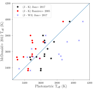
The Ramírez, & Meléndez (2005) temperature relations are systematically offset from the adopted temperatures while the Jian et al. (2017) results appear consistent with our adopted temperatures from SED fits. The average difference and standard deviation for the two color-$T_{\mathrm{eff}}$ relations from Jian et al. (2017) are 35 K $\pm$ 117 K for J - K_s and 89 K $\pm$ 173 K for J - W3. We therefore adopt the McDonald et al. (2012) temperatures with uncertainties of $\pm$ 100 K.

3.2 Surface Gravity

Next, we calculated the surface gravity for each star in our sample using Eq. 1:

$$\mathrm{Log}(g/g_{\odot})=\mathrm{Log}(M/M_{\odot})-\mathrm{Log}(L/L_{\odot})+\mathrm{4Log}(T/T_{\odot})$$ (1)

In equation 1, M is the stellar mass, L is the luminosity, and T is the effective temperature. The luminosity of each star was derived using the K magnitude from DIRBE or 2MASS (Hauser et al., 1998; Smith et al., 2004) (transformed to Johnson K), distances using Gaia DR2 parallaxes (Gaia Collaboration et al., 2018) from Bailer-Jones et al. (2018), and K band bolemetric corrections from Bessell et al. (1998). Due to the spacing in the grid of bolometric corrections for the M giant stars, we adopt an uncertainty of $\Delta$BC_K = $\pm$ 0.2 when calculating the luminosity uncertainty. For stars with no available Gaia DR2 parallax, Hipparcos parallax measurements (ESA, 1997) were used instead to calculate the luminosity.

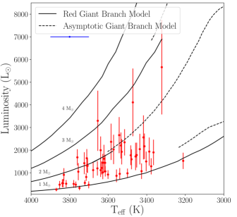
With known luminosities and effective temperatures we compared our results to stellar evolutionary tracks from Bertelli et al. (2008, 2009). Specifically, we assumed our M giants have metallicities consistent with the solar Z and used the tracks with Y = 0.30 and Z = 0.017. The effective temperature and luminosities for each star were compared to stellar evolution tracks at various masses and the model that most closely matched the two parameters was adopted as the stellar mass of the star. The models between 0.8 - 2.2 M_⊙ varied in steps of 0.1 M_⊙ and 2.5 - 4 M_⊙ varied in steps of 0.5 M_⊙. We tested the uncertainty on the mass calculations by conducting a Monte Carlos simulation for a typical star in our sample, HD 164448 ($T_{\mathrm{eff}}$ = 3634, L = 1210 L_⊙, and mass = 1.7 M_⊙). We re-computed the effective temperature and luminosity using a Gaussian number with the standard deviation set to the uncertainties, recalculated the mass, and repeated 5,000 iterations. The standard deviation on the distribution was 0.32 M_⊙. Since the stars with larger masses have have sparser mass coverage, we estimated the uncertainty on each star to $\delta$M = $\pm$0.5 M_⊙ when calculating the log(g). Fig. 3 comparison of the luminosity and effective temperature to some stellar evolutionary tracks. We find most stars in our sample range between 1 M_⊙ and 2 M_⊙. Finally log(g) values are calculated with Eq. 1 with uncertainties from each intrinsic parameter propagated and the average log(g) uncertainty is 0.20 $\pm$ 0.03 for the sample.

Figure 3: A HR diagram for the M giant sample. Black lines are red giant branch stellar evolution tracks and dashed lines are asymptotic giant branch stellar evolution tracks, both from Bertelli et al. (2008, 2009). A representative effective temperature error represented by a blue bar.

3.3 [Fe/H] and Microturbulence

The [Fe/H] abundance for each star was measured using Fe I lines in the optical echelle spectra between 7400 Å - 7580 Å and from 8600 Å to 8700 Å. The chosen spectral regions have both minimal telluric contamination and no strong TiO molecular bands. Fe I lines used between 7400 Å - 7580 Å have previously been used to determine Fe I abundances in M giant stars (Smith, & Lambert, 1990; Chou et al., 2007). We chose atomic line information (e.g. excitation potential) from the Kurucz database and lines from Chou et al. (2007).

Table 2: Atomic Ti I and Fe I lines

Species	Wavelength	$\xi$	log(gf)
	(Å)	(eV)
Ti I	7402.675	3.179	-0.973
Ti I	7416.99	1.067	-3.345
Ti I	7423.183	1.443	-2.612
Ti I	7432.67	1.460	-2.751
Ti I	7456.584	0.818	-3.468
Ti I	7469.938	0.836	-3.268
Ti I	7491.362	0.826	-3.553
Fe I	7440.911	4.913	-0.572
Fe I	7443.022	4.186	-1.75
Fe I	7445.749	4.256	-0.103
Fe I	7447.384	4.958	-1.011
Fe I	7461.519	2.559	-3.53
Fe I	7476.375	4.795	-1.55
Fe I	7498.53	4.143	-2.19
Fe I	7507.265	4.415	-0.972
Fe I	7511.018	4.178	0.187
Fe I	7531.143	4.371	-0.67
Fe I	7547.896	5.099	-1.147
Fe I	7568.898	4.283	-0.822
Fe I	8611.803	2.845	-1.86
Fe I	8674.746	2.831	-1.81
Fe I	8698.706	2.990	-3.517
Fe I	8699.455	4.955	-0.469

To test our linelist choices, we measured equivalent widths in the Sun (Wallace et al., 2011) and Arcturus (Hinkle et al., 2000) using visible solar atlases for all detectable Fe I lines in the spectral region. The log(gf) values were adjusted for some Fe I lines to match the solar and Arcturus abundance. To avoid using spectral lines subjected to large systematic effects with temperature or luminosity, any line that could not simultaneously reproduce the abundance in Arcturus and in the Sun was removed from the linelist. We derived an abundance of A(Fe I) = 7.51 $\pm$ 0.05 (st.dev.) for the Sun and A(Fe I) = 6.97 $\pm$ 0.05 (st.dev.) for Arcturus with the linelist in Table 2, consistent with the values from Asplund et al. (2009) and Ramírez, & Allende Prieto (2011) respectively.

The Fe I lines were examined in the R $\sim$ 100,000 spectra and R $\sim$ 30,000 ARCES spectra and lines with significant blending were removed from the linelist. The final set of lines with astrophysical log(gf) values are listed in Table 2. The lines beyond 7580 Å were not available in the TOU spectra while three lines heavily blended in the ARCES spectra were measurable in the higher resolution TOU spectra. Those lines are indicated in Table 2.

3.3.1 Determining [Fe/H] and Microturbulence

Equivalent width measurements were then performed for all stars using splot task within IRAF. Iron abundances for each line were calculated using the abfind routine with MOOG spectral synthesis software (Sneden 1973; V. 2017) and MARCS model atmospheres (Gustafsson et al., 2008). Models were initially set to the [Fe/H] = 0 and a microturbulence value of 2.0 km s^-1. The best microturbulence value was calculated by conducting a grid search in steps of 0.01 km s^-1 and determining which microturbulence value minimized the slope of the A(Fe I) abundance and reduced equivalent width (log(EW/$\lambda$)) for all Fe I lines measured. The process was repeated with a new atmospheric model, created with the average A(Fe I) abundance and microturbulence from the last iteration. The iterations were stopped and the final values chosen, when the A(Fe I) abundance did not changed by more than 0.01 dex. Typically only two to three iterations were necessary. The final set of atmospheric parameters is given in Table 3.

The standard deviation calculated from the abundances derived for individual Fe I lines determined was adopted as the statistical [Fe/H] uncertainty. Additionally, uncertainties in the effective temperature and surface gravity were calculated for five sample stars, then applied the average uncertainty to the rest of the Fe abundances. For the five stars, models at $\pm$ 100 K and $\pm$ 0.20 in log(g) were created individually, the new A(Fe I) computed, and the difference adopted as the uncertainty. The atmospheric parameter uncertainties were added in quadrature with the uncertainty on the fit. The final average $\delta$A(Fe I) is $\pm$ 0.16 dex. The microturbulence uncertainty was calculated using the 1$\sigma$ uncertainty on the best fitting linear line to the A(Fe I) abundance and reduced equivalent width (log(EW/$\lambda$)), obtained from the covariance matrix. The uncertainty in the microturbulence is the difference between the grid search result and the microturbulence corresponding to the 1$\sigma$ slope. The average difference is $<\Delta\chi>$ = 0.15 $\pm$ 0.03 (s.t.dev) for the five stars. We used the average 2$\sigma$ value of 0.30 kms^-1 as the uncertainty estimate for the entire sample to ensure no stars were beyond this limit in our sample.

Table 3: M Giant Stellar Parameters and Abundances

HD	$T_{\mathrm{eff}}$	log(g)	A(Fe I)	[Fe/H]	$\xi$	A(O)	A(35Cl)	A(Ca)	A(Ti)
Number	(K)				(km s-1)
5111	3636	0.91	7.51	0.01	2.13	$\cdots$	4.98	6.29	4.93
15594	3436	0.43	7.40	-0.10	1.71	$\cdots$	4.71	6.01	4.67
19258	3601	0.79	7.29	-0.21	1.89	$\cdots$	4.73	6.18	4.63
25000	3479	0.56	7.52	0.02	1.91	$\cdots$	4.88	6.24	4.87
30634	3714	0.94	7.26	-0.24	2.01	8.46	4.43	5.85	4.63
31072	3779	1.11	7.46	-0.04	2.13	8.64	5.15	6.22	4.78
35067	3701	1.00	7.50	0.00	2.00	8.58	4.95	6.11	4.79
84181	3622	0.71	7.35	-0.15	1.87	$\cdots$	5.09	6.22	4.74
99592	3365	0.37	7.28	-0.22	1.82	$\cdots$	4.56	5.62	4.65
102159	3387	0.40	7.44	-0.06	2.22	$\cdots$	4.69	6.01	4.69

Note. — (This table is available in its entirety in machine-readable form.)

4 Abundance Analysis

4.1 Abundance Derivations

Abundances were derived using MOOG spectral synthesis software (Sneden 1973; v. 2017) with MARCS 1-D atmospheric models (Gustafsson et al., 2008). We adopted the linelist from Maas et al. (2016) to determine abundances from the IR spectra. In the previous studies, CNO abundances were derived using CH, OH, and NH molecular features at 3.7 $\mu$m. However, the very weak CH features were too significantly blended to discern in the lower resolution CSHELL spectra. The molecular equilibrium for molecules containing CNO depends on the abundances of all three species. Without independent methods to determine all CNO abundances we focus on determining only the Cl and Ca abundances from our IR spectra. Ca provides an accessible $\alpha$ element for comparison with Cl and abundance measurements in disk stars using Ca I features at 3.7 $\mu$m are consistent with abundances from optical lines (Maas et al., 2016).

We determined which abundance minimized $\chi^{2}$ for the multiple sets of synthetic spectra and observed IR spectrum of each star. The $\chi^{2}$ minimization was done over the shaded regions in Fig. 1 to find the abundances of Ca and Cl. We avoided the two blended Ca features since we are not deriving CNO abundances. A grid search was performed using the synthetic spectra created over a range of Cl and Ca abundances. The best fitting abundances for the two regions are given in Table 3. We use Asplund et al. (2009) as the solar reference for all elements except for Cl in which we use the meteoric value from Lodders et al. (2009), consistent with the methodology of Maas et al. (2016).

4.2 Oxygen Abundance Derivations

Oxygen abundances are necessary to meaningfully compare our results to PN and H II regions. While OH lines are present in the L band spectra, determining abundances from them without carbon abundances is difficult due to the CNO molecular equilibrium. We therefore use the forbidden oxygen line at 6300 Å to determine oxygen abundances in our stars. The 6300 Å region is on the edge of a TiO band centered at $\sim$ 6150 Å. A linelist was created using the [O I] line, nearby Fe I lines, and TiO lines from the $\delta$ transition taken from Plez (1998). Due to the number of of TiO lines, only lines with log(gf) values above –0.5 and excitation potentials lower than 1 eV were selected. Additional lines contributed little to the resulting synthetic spectra while increasing computation time. Solar Ti isotope fractions were assumed and adopted from Asplund et al. (2009). Synthetic spectra were created using MOOG (Sneden 1973; v. 2017) and MARCS atmospheric models (Gustafsson et al., 2008). The linelist was tested on Arcturus and reproduces the oxygen abundance and Fe abundance from Ramírez, & Allende Prieto (2011).

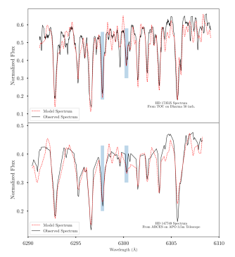
The stellar continuum was difficult to determine due to the TiO molecular lines blanketing the spectral region. First, we used the continuum task in IRAF and normalized to the apparent continuum in the [O I] spectral region. A synthetic spectrum with only the TiO component was created and fit with a spline function. The initially divided spectra in our sample were then divided by the TiO spline fit to re-introduce the TiO component across the wavelength range of interest. Best fit spectra were determined by performing a $\chi^{2}$ minimization over the [O I] line region and a nearby Fe I line to constrain the fit to the continuum from TiO. A grid of synthetic spectra that varied in oxygen abundances in 0.01 steps were created and fit; re-calculating the TiO contribution to the continuum at every step. The $\chi$ values were also weighted by the TiO continuum contribution to ensure the minimum $\chi^{2}$ value was not related to the decreasing flux with higher O abundances, and stronger TiO features. Examples of the best fitting spectra for HD 147749 and HD 173525 are shown in Fig. 4. Abundance uncertainties from the atmospheric parameters were calculated using the same methodology as subsection 4.3.2.

Figure 4: Both panels show synthetic spectra fits to observed data. The blue boxes show the features chosen for the $\chi^{2}$ minimization. Top Panel: HD 173525 spectrum fit. The star was observed using TOU on the Dharma 50” telescope. Bottom Panel: HD 147749 spectrum fit. The star was observed using ARCES on the APO 3.5m telescope.

Figure 5: [O/Fe] ratios vs. [Fe/H]. Black stars are abundance ratios from this work and grey circles are from Bensby et al. (2014). The blue point give representative error bars on the Cl and O abundances.

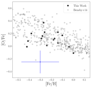
Additionally, telluric lines are present near the spectral region containing the [O I] feature. We did not perform a telluric correction for the optical spectra and although we do not see any anomalously strong [O I] features or blends with un-identified lines, contamination still may be present. Only a subsample of our observed stars with $T_{\mathrm{eff}}$ $>$ 3700 K have O abundances measured. Below this temperature, the TiO features begin dominating all other features and systematic uncertainties from modeling TiO continuum, specifically the linelist and atmospheric parameters, become significant. We therefore measured O abundances in the 15 warmest stars from the original sample. The oxygen abundances are listed in Table 3 with average uncertainties listed in Table 4. We also compare our derived oxygen abundances to [O/Fe] ratios in FGK stars from Bensby et al. (2014) in Fig. 5. We found our [O/Fe] ratios agree with ratios from Bensby et al. (2014), providing evidence our methodology provides sufficiently accurate results to compare to nebular abundances.

4.3 Uncertainty Analysis

4.3.1 Uncertainty from Fit

The noise in the final, reduced, 1D spectra come from multiple sources including the original counts, division with a telluric spectrum, and division by a flat-field spectrum. We devised multiple similar methodologies to account for this source of uncertainty when fitting synthetic spectra to the data.

The uncertainty in the Cl and Ca spectral synthesis fit was estimated through a Monte Carlo simulation. A grid of synthetic spectra with an individual element abundance change in steps of 0.01 dex for each spectrum in the grid, was created for Ca and ³⁵Cl. A new spectrum was created by generating Gaussian random numbers for each pixel flux value with the mean value the original measured flux and a standard deviation equal to the signal-to-noise ratio of the data. The best fitting elemental abundances were calculated for each adjusted stellar spectrum. The process was repeated for 100,000 iterations and the 16$\%$ and 84$\%$ values of the posterior distribution of the Monte Carlo simulation were adopted as the uncertainty on the fit. For Ti and Fe, abundances were individually derived for multiple lines with equivalent width measurements. The average of the lines was taken as the stellar abundance and the standard deviation as the uncertainty due to the fit.

4.3.2 Uncertainty from Atmospheric Parameters

The uncertainty on each abundance measurement due to noise in the spectra and uncertainty in the atmospheric parameters, assumed to be independent, was added in quadrature. The uncertainty for each abundance due to uncertainty on the adopted atmospheric parameters was calculated by using new atmospheric models. We varied one atmospheric parameter by 1$\sigma$ (e.g. $T_{\mathrm{eff}}$) while the others were held constant to the adopted values, created a new atmospheric model, then new abundances were derived. The best fitting abundances were found by minimizing the $\chi^{2}$ between the model fit and the synthetic spectra, the same procedure described in subsection 4.1. The 1$\sigma$ uncertainties from the atmospheric parameters is defined as the difference between the abundance derived and the atmospheric models with adjusted atmospheric parameters and are listed in Table 4.

Table 4: M Giant Abundance Uncertainty Averages

Uncertainty	$\delta$A(O)	$\delta$A(35Cl)	$\delta$A(Ca)	$\delta$A(Ti)
Source	(dex)	(dex)	(dex)	(dex)
$T_{\mathrm{eff}}$	0.04	0.20	0.04	0.09
log(g)	0.04	0.01	0.03	0.04
$\mathrm{[Fe/H]}$	0.07	0.06	0.17	0.09
$\xi$	0.15	0.00	0.07	0.10
Fit	0.03	0.05	0.02	0.10
Tot. Uncertainty	0.18	0.21	0.19	0.19

4.3.3 Uncertainty with Effective Temperature

No NLTE calculations are available for the L band HCl transitions. Additionally, blends with weak, un-identified molecular features may impact our abundances. In both scenarios, the systematic uncertainty will likely change as a function of the effective temperature. Maas et al. (2016) found no relationship between ³⁵Cl, C, O, N, Si, and Ca with $T_{\mathrm{eff}}$ using abundances from the same L band region. We test those results by examining the relationship between the adopted $T_{\mathrm{eff}}$ and abundance with the our larger sample of 52 M giants.

To check for consistency within our abundance measurements, we examined how the atmospheric parameters correlated each another. While most atmospheric parameters are uncorrelated, there is a relationship between the effective temperature and [Fe/H], where cooler stars are more metal rich compared to the warmer stars in the sample. The average abundance for stars with effective temperatures cooler than 3500 K is $<$[Fe/H]$>$ = –0.09 while the stars with $<$[Fe/H]$>$ = –0.19 for stars warmer than 3500 K. The offset may be due to unknown systematics with the [Fe/H] calculations, such as unknown blends with molecular lines, from problems with the atmospheric models, or due to a stellar evolution effect. Higher metallicity stars evolve with relatively cooler effective temperatures on the red giant branch (e.g. Bertelli et al. 2008). Therefore, we may expect a metallicity trend with effective temperature in our sample since the cooler stars may be more likely to be metal-rich when selected by effective temperature and magnitude.

One way to determine the cause of [Fe/H] and $T_{\mathrm{eff}}$ relation is to look at the relationship between other elements with effective temperature in the M giant sample. We plot the effective temperature against the [³⁵Cl/Fe], [Ca/Fe], and [Ti/Fe] ratios in Fig. 6. We find both [Ti/Fe] and [³⁵Cl/Fe] increase with increasing effective temperature. To further understand this relationship, we split the sample into three metallicity bins and do a bootstrap estimate to determine the relationship between abundance and effective temperature. The bin sizes were chosen to approximately match the region before the [Ti/Fe] slope increases in Bensby et al. (2014). Bin sizes were also chosen to cover the necessary $T_{\mathrm{eff}}$ range and finally to probe roughly different regimes in the MARCS [Fe/H] grid spacing (–0.5, –0.25, and solar metallicity). We fit each bin with a linear line and the bootstrap was performed with 10,000 iterations. The linear fit was performed with a Levenburg-Marquardt algorithm and soft l1 loss smoothing approximation to remove outliers. The resulting slopes and their uncertainties are found in Table 5. We find the [Ti/Fe] and [Ca/Fe] ratios, at similar [Fe/H] ratios, are approximately constant over the $T_{\mathrm{eff}}$, as shown in Fig. 6. When only the stars with $T_{\mathrm{eff}}$ $>$ 3500 K are fit, the slopes become statistically consistent with zero.

Figure 6: Plots of [³⁵Cl/Fe] (top), [Ti/Fe] (middle), and [Ca/Fe] (bottom) versus $T_{\mathrm{eff}}$. Blue crosses are representative error bars. Left most plot shows the entire sample of stars. Next plots are binned in [Fe/H] $>$ –0.1, –0.3 $<$ [Fe/H] $<$ –0.1, and –0.6 $<$ [Fe/H] $<$ –0.3 respectively. Solid black line is best linear fit to the data and the red lines in each bin represent 3000 bootstrap fits. The slopes for each parameter are given in Table 5.

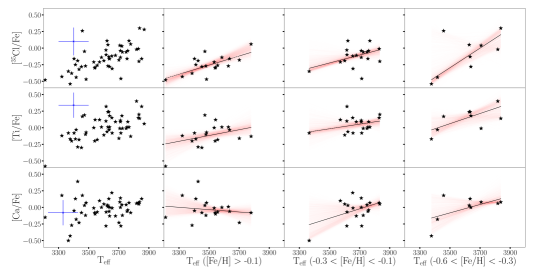
Only the high metallicity [³⁵Cl/Fe] bin has a significant non-zero slope. However, the ³⁵Cl abundance increases with effective temperature, which is not consistent with unknown molecular blends becoming stronger as effective temperature decreases, artificially enhancing the H³⁵Cl line strength. The warmest star in the bin has a large [³⁵Cl/Fe] ratio and has a high leverage on the fit, even when the coolest stars are removed. For the Fe I lines, if an unidentified molecular feature was blended with either the Ti I features, Fe I features, or the H³⁵Cl molecular feature, a relationship with effective temperature should be especially present in the highest metallicity bin, in which no clear trend is present in Fig. 6.

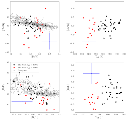
³⁵Cl, Ti, and Ca have different average abundance ratios to Fe in each bin. Since Ti and Ca surface abundances should not be affected by stellar evolutionary effects, we expect the abundance ratios of the M giants to be similar to FGK stars in the disk. We can compare the [Ti/Fe] and [Ca/Fe] ratios in our sample with Bensby et al. (2014) abundances from FGK disk stars, shown in Fig 7. The left panels compare the abundances while the right panels show the [X/Fe] ratios versus effective temperature for the M giant sample from this work.

We find overall agreement between [Ti/Fe] and [Ca/Fe] between both samples, although due to the large uncertainties we cannot distinguish if stars are consistent with thin or thick disk abundance ratios. However, the coolest stars in our sample are systematically lower in the [Ti/Fe] sample. We also calculate the average [Ti/Fe] in the different metallicity bins for our sample and also Bensby et al. (2014), with the results shown in Table 6. The averages in Table 6 demonstrate that the coolest stars, below 3500 K, are systematically offset and removing them from the sample brings the abundances more in line with literature values. M giant [Ca/Fe] ratios appear systematically lower compared to the abundances of Bensby et al. (2014). Only one Ca line is used and difficulties defining the continuum, or problems with the higher excitation energy lines in cooler models, may introduce the offset with Bensby et al. (2014) results. We note the scatter in [Ca/Fe] ratios is larger for the cooler stars, demonstrated in both panels showing [Ca/Fe] ratios in Fig. 7.

Table 5: Slopes from Linear fits to [X/Fe] vs $T_{\mathrm{eff}}$ for Fig. 6.

[X/Fe]	[Fe/H]	All Stars	Stars with $T_{\mathrm{eff}}$ $>$ 3500K
	Bin	Slope	Slope
		(dex 100K-1)	(dex 100K-1)
$\mathrm{[Cl/Fe]}$	[–0.6, –0.3]	0.10 $\pm$ 0.08	0.1 $\pm$ 0.4
$\mathrm{[Cl/Fe]}$	[–0.3, –0.1]	0.05 $\pm$ 0.02	0.03 $\pm$ 0.04
$\mathrm{[Cl/Fe]}$	[–0.1, 0.2]	0.09 $\pm$ 0.02	0.14 $\pm$ 0.04
$\mathrm{[Ti/Fe]}$	[–0.6, –0.3]	0.06 $\pm$ 0.04	–0.01 $\pm$ 0.14
$\mathrm{[Ti/Fe]}$	[–0.3, –0.1]	0.03 $\pm$ 0.03	0.02 $\pm$ 0.05
$\mathrm{[Ti/Fe]}$	[–0.1, 0.1]	0.04 $\pm$ 0.03	0.00 $\pm$ 0.05
$\mathrm{[Ca/Fe]}$	[–0.6, –0.3]	0.06 $\pm$ 0.05	0.01 $\pm$ 0.11
$\mathrm{[Ca/Fe]}$	[–0.3,–0.1]	0.06 $\pm$ 0.05	0.01 $\pm$ 0.04
$\mathrm{[Ca/Fe]}$	[–0.1, 0.2]	–0.02 $\pm$ 0.03	–0.03 $\pm$ 0.03

Figure 7: Left: [Ca/Fe] and [Ti/Fe] vs. [Fe/H] ratios. The stars are from the M giant sample, red stars have $T_{\mathrm{eff}}$ $<$ 3500 K while black stars have $T_{\mathrm{eff}}$ $>$ 3500 K. The gray circles are from Bensby et al. (2014). Right: The [Ca/Fe] and [Ti/Fe] ratios vs. effective temperature. In all plots, a blue point is shown with representative error bars.

From a comparisons to other abundances we suggest the [Fe/H] dependence on effective temperature is due to selection effects; cooler M giants are more likely to be metal-rich. However, the coolest stars, at temperatures of $\sim$ 3500 K and cooler, are offset in [Ti/Fe] and [Ca/Fe] from typical disk abundances. Possible problems with the atmospheric models may be affecting the [Fe/H] derivations in the coolest stars in the sample. The interpolation code for the MARCS models was not used for stars at 3500 K and cooler and deviations from measured atmospheric parameters to those adopted with the sparser grid of models may be causing the offsets. When interpreting the data, we will only analyze stars with $T_{\mathrm{eff}}$ $>$ 3500 K, and distinguish abundances from warmer and cooler stars in figures.

Table 6: Average Ti Abundances

[Fe/H] Bins	This Work	This Work	Bensby+14
	Full Sample	$T_{\mathrm{eff}}$ $>$ 3500 K
	$<$[Ti/Fe]$>$	$<$[Ti/Fe]$>$	$<$[Ti/Fe]$>$
[–0.1, 0.25]	–0.11	–0.05	0.02
$\mathrm{[}$–0.3, –0.1$\mathrm{]}$	0.05	0.06	0.08
$\mathrm{[}$–0.6, –0.3$\mathrm{]}$	0.13	0.20	0.17

5 Discussion

5.1 Cl Evolution in the Galaxy

The Cl abundances from this work can be found in Fig. 8. The [Cl/Fe] abundances were calculated using the A(³⁵Cl) abundances from Table 3 and assuming a ³⁵Cl/³⁷Cl = 2.66 isotope ratio, the average from the sample of Maas & Pilachowski (2018). Though the Cl isotope ratio may vary in our sample, the uncertainty from the isotope ratio is less significant than the uncertainty from the effective temperature. For example, for an A(³⁵Cl) = 5.13, the A(Cl) for ³⁵Cl/³⁷Cl = 2.08, 2.66, and 3.24, is 5.30, 5.27, and 5.25; while the uncertainty from varying $T_{\mathrm{eff}}$ $\pm$ 100 is 0.20 dex.

Multiple Cl chemical evolution models are compared to our observed [Cl/Fe] ratios in Fig. 8. A model from Kobayashi et al. (2011) includes hypernovae, CCSNe, Type Ia SN, and AGB star yields and is tuned to match the solar neighborhood. A similar model was created by Prantzos et al. (2018) with one key difference; the inclusion of yields from rotating massive stars. Finally, Ritter et al. (2018) constructed chemical evolution models with the yields of enhanced from C-O shell mergers for a certain fraction of the stars in the Galaxy. We plot the only models from Ritter et al. (2018) that are close to the measured [Cl/Fe] values in the data, the chemical evolution models with 0$\%$ of stars undergoing C-O shell mergers and the 10$\%$ model, in Fig. 8. All chemical evolution models plotted initially assumed A(Cl)$|_{\odot}$ = 5.50, which we adjusted to match the value of A(Cl)$|_{\odot}$ = 5.25 from Lodders et al. (2009) and adopted for our data. We note the chemical evolution models compared to our sample were tuned for the solar neighborhood which approximately corresponds to the sample of stars collected. The most distant star in our sample is HD 132917 at a distance of 836 pc and the median distance is 367 pc.

Figure 8: [Cl/Fe] abundances versus [Fe/H] for M giant stars. The black stars denote abundances in stars with $T_{\mathrm{eff}}$ $>$ 3500 K and red stars denote stars with $T_{\mathrm{eff}}$ $<$ 3500 K, for stars listed in Table 3. Grey circles are for [Cl/Fe] abundances from Maas et al. (2016). The [Cl/Fe] ratio was calculated with ³⁵Cl abundances with an isotope ratio of ³⁵Cl/³⁷Cl = 2.66 assumed from Maas & Pilachowski (2018). Chemical evolution models from Kobayashi et al. (2011) (blue dashed line), Prantzos et al. (2018) (purple solid line), and Ritter et al. (2018) (orange dot-dashed lines) are included. The model from Ritter et al. (2018) with larger [Cl/Fe] ratio assumes a C-O shell merger rate of 10$\%$ and the other model assumes no stars undergo a C-O shell merger. Dashed black lines are solar abundances.

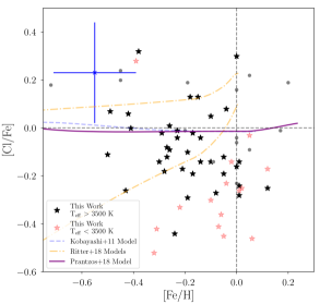
From initial inspection, we note the chemical evolution models from Kobayashi et al. (2011) and Prantzos et al. (2018) broadly agree with [Cl/Fe] ratios in our sample, and may slightly over-produce Cl in the solar neighborhood. Both models predict a nearly constant [Cl/Fe] vs. [Fe/H], with a slope of $\sim$ 0 for an [Cl/Fe] $\sim$ –0.02 dex over the range –0.6 $<$ [Fe/H] $<$ 0.3. To test if our abundances match this value, we took the average of our sample and the averages for the three metallicity bins discussed in subsection 4.3.3. We only compute averages and compare results of the $T_{\mathrm{eff}}$ $>$ 3500 K sample, as the cooler stars appears offset at all metallicities relative to the rest of the sample. As discussed in subsection 4.3.3, the stars with $T_{\mathrm{eff}}$ $<$ 3500 K may not have reliable abundances and are therefore excluded from our statistical analysis.

The average abundance for all warm stars is $<$[Cl/Fe]$>$ = –0.08 $\pm$ 0.16 (s.t.dev), consistent with chemical evolution models. The average abundance ratios from each bin are given in Table 7 and we find all bins and the total sample averages are consistent with predictions and within one standard deviation of the model [Cl/Fe] ratio. Finally, we note that no model from Ritter et al. (2018) is able to match the slope or [Cl/Fe] ratio over the [Fe/H] range of our data.

The [Cl/Fe] ratio also appears to decrease with increasing metallicity from inspection of Fig. 8 and from the binned averages in Table 7. No slope for the [Cl/Fe] ratio vs. [Fe/H] ratio is expected from the chemical evolution models of Kobayashi et al. (2011); Prantzos et al. (2018). We used a Monte Carlo simulation to determine the significance of the [Cl/Fe] vs. [Fe/H] slope. We generated random Gaussian numbers with an average value equal to the measured abundance ratio ([Cl/Fe]) with a standard deviation equal to the measurement uncertainty. We then determined a best fitting linear model using a Levenberg-Marquardt least-square method. The process was repeated 50,000 times with a new set of randomly generated data created for each iteration. We find the most probable slope is negative, in the case simulating [Cl/Fe] ratios only the average slope is –0.22 $\pm$ 0.23. The best fitting Levenberg-Marquardt least-square fit to the data yields an uncertainty on the slope with -0.22 $\pm$ 0.17, similar to the bootstrap method result. We also note the uncertainty on the x-axis flattens out the fit and drives the slope closer to zero. We fit the data using a SIMEX algorithm and find a slope of –0.38 $\pm$ 0.27 and a p-value of 0.16. In both cases the slope is negative but within 1-2 $\sigma$ of $\sim$0. Therefore, our abundances suggests a small slope appears to exist in the [Cl/Fe] vs. [Fe/H] data, for stars with $T_{\mathrm{eff}}$ $>$ 3500 K, but is not statistically significant given the uncertainties on each measurement.

Table 7: Average [Cl/Fe] Abundances

[Fe/H]	$<$[Cl/Fe]$>$	$\sigma$([Cl/Fe])	Stars
Range			in Bin
Full Sample	–0.08	0.16	34
$\mathrm{[}$–0.1, 0.25$\mathrm{]}$	–0.13	0.19	10
$\mathrm{[}$–0.3, –0.1$\mathrm{]}$	–0.09	0.14	18
$\mathrm{[}$–0.5, –0.3$\mathrm{]}$	0.01	0.18	6

Note. — All stars have $T_{\mathrm{eff}}$ $>$ 3500 K

5.2 Comparing Cl Abundances to Ca and Ti

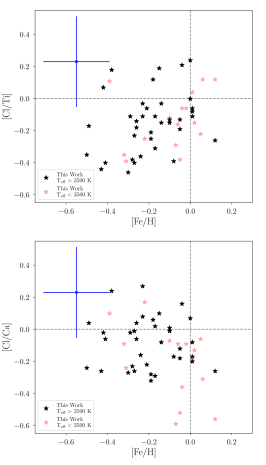
We compare chlorine to to both Ti and Ca abundances measured in our M giants. Both elements are thought to be $\alpha$ elements produced through explosive burning in massive stars with non-trivial production from Type Ia SN. While chemical evolution models accurately reproduce Ca abundances they fail to match Ti in the solar neighborhood adding uncertainty to the CCSNe to Type Ia fraction for Ti (Nomoto et al., 2013; Prantzos et al., 2018). We note that Ca shows a shallow decrease in [Ca/Fe] as [Fe/H] as shown in Fig. 7. We examine [Cl/Ca] and [Ca/Ti] in Fig. 9. While scatter is significant, there is no slope in the [Cl/Ca] abundance ratios and the [Cl/Ti] ratio increases with [Fe/H]. The [Cl/Ca] ratio in particular indicates Cl is made in similar CCSNe to Type Ia SN ratios as Ca over our metallicity range.

Figure 9: Top Panel: [Cl/Ti] ratio versus [Fe/H]. Bottom Panel: [Cl/Ca] ratio versus [Fe/H]. The [Cl/Fe] ratio was calculated with ³⁵Cl abundances with an isotope ratio of ³⁵Cl/³⁷Cl = 2.66 assumed from Maas & Pilachowski (2018). In both plots, the black stars shapes indicate stars with $T_{\mathrm{eff}}$ $>$ 3500 K and red stars indicate $T_{\mathrm{eff}}$ $<$ 3500 K. The single blue cross in each plot give representative error bars.

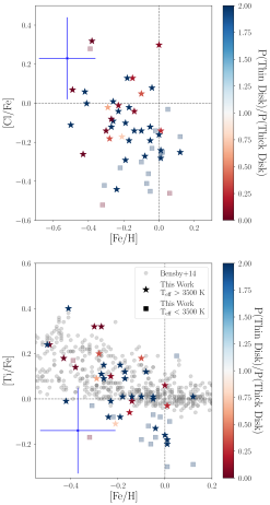
We also calculated the UVW velocity of our sample using Gaia distances and proper motions (Gaia Collaboration et al., 2018). Radial velocity measurements were adopted primarily from Famaey et al. (2005). The Gaia data, with RA, DEC, and radial velocity measurements were accessed using the SIMBAD database. The UVW velocities were calculated using a python based calculator. The thin disk, thick disk, and halo membership probabilities based on the kinematics of each star were calculated using the same methodology as Ramírez et al. (2013). The thin/thick disk probabilities with Cl and Ti abundances are compared in Fig. 10 and the probabilities are given in Table 8.

Table 8: M giant Fundamental Parameters and UVW Velocities

HD	Lum.	$\delta$Lum.	Distance	Mass	U	V	W	P(Thin/Thick)
Num	(L⊙)	(L⊙)	(pc.)	(M⊙)	(km s-1)	(km s-1)	(km s-1)	Ratio
5111	530	170	351	1	84.5	-69.6	-12.7	0.3
15594	2040	670	383	1.6	-58.6	8.5	16.0	51.5
19258	920	190	349	1.4	55.9	-49.0	48.6	0.8
25000	1600	440	372	1.6	47.4	-33.1	-10.5	25.3
30634	810	170	336	1.5	10.6	-25.1	-49.7	7.0

Note. — (This table is available in its entirety in machine-readable form.)

We identify 17 stars in our sample as probable thick disk members with probability ratios of P_thin/P_thick $<$ 1. The average iron abundance for thin and thick disk stars with $T_{\mathrm{eff}}$ $>$ 3500 K are $<$[Fe/H]$>$ = –0.17 $\pm$ 0.15 and $<$[Fe/H]$>$ = –0.23 $\pm$ 0.15 respectively. In the top panel of Fig. 10 we note that the thin and thick disk stars have similar [Ti/Fe] ratios at [Fe/H] $>$ –0.20 dex. Beyond this metallicity the [Ti/Fe] ratios are larger than the [Fe/H] in Fig. 10. For Cl, the difference between [Cl/Fe] abundances between thin disk and thick disk members at any [Fe/H] is not significant. The consistency between both thin and thick disk populations suggests that Cl production is significant enough in Type Ia SN to cause no detectable difference in either population for our sample, although our sample sizes are small and uncertainties relatively large.

Figure 10: Top Panel: [Cl/Fe] abundance versus [Fe/H] for M giant stars. The [Cl/Fe] ratio was calculated with ³⁵Cl abundances with an isotope ratio of ³⁵Cl/³⁷Cl = 2.66 assumed from Maas & Pilachowski (2018). Bottom Panel: [Ti/Fe] ratios from our sample are compared to abundances from Bensby et al. (2014) (grey points). In both plots, the dashed black lines are solar abundances and the stars shapes represent stars with $T_{\mathrm{eff}}$ $>$ 3500 K and squares are $T_{\mathrm{eff}}$ $<$ 3500 K. The single blue cross in each plot give representative error bars. Thin to thick disk probability ratios are given in the color bar.

5.3 Stellar Cl Abundances Compared to Nebular Cl Abundances

We compare the derived O and Cl abundances in stars to measurements in H II regions and PNs in Fig. 11. We select H II and PN nebular abundances from Henry et al. (2004); Delgado-Inglada et al. (2015); Arellano-Córdova et al. (2020). Since all of our target stars have distances within 1 kpc from the Sun, we select objects with galactocentric radii between 6 kpc and 11 kpc. The cut ensures we are not comparing the chemical evolution of different regions of the Galaxy to our sample. The nebular and stellar A(O) and A(Cl) abundances are plotted in Fig. 11.

Figure 11: A(Cl) vs. A(O) for nebular abundance data and from our sample of stars. Red squares are from Arellano-Córdova et al. (2020), orange x shapes are from Delgado-Inglada et al. (2015), grey circles are from Henry et al. (2004), blue diamonds are from Maas et al. (2016), and black stars are from this work. The A(Cl) abundances use the A(³⁵Cl) abundances and adopt an isotope ratio of ³⁵Cl/³⁷Cl = 2.66 from Maas & Pilachowski (2018) to calculate total Cl abundances.

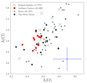
We find the stellar abundances broadly agree with the H II region and PN A(Cl) measurements, although there is significant scatter in the data. The consistent results suggests both sets of astrophysical objects accurately probe the Cl abundance, providing evidence no significant systematic uncertainties affect the Cl abundances in stars measured with HCl features. We also find A(Cl) and A(O) increasing in all samples, suggesting both A(Cl) and A(O) are produced in massive stars and are made in lockstep, providing additional evidence the primary source of Cl is from CCSNe. We note the scatter and uncertainty on the Cl abundances are large, making a search for secondary behavior with respect to oxygen difficult. A simple linear regression for all objects in Fig. 11, excluding objects with A(Cl) $<$ 4.75 to remove outliers, finds a slope of 1.03 $\pm$ 1.01. More precise measurements in more stars are needed to further constrain the evolution of Cl but the general agreement between nebular abundances and stellar abundances are promising for the accuracy of stellar Cl abundance measurements.

6 Conclusions

The Galactic chemical evolution and nucleosynthesis of Cl was examined a sample of 52 M giants. Atmospheric parameters were derived using optical echelle spectra of our M giants with $T_{\mathrm{eff}}$ from McDonald et al. (2012), log(g) using Gaia DR2 parallax measurements, [Fe/H] and microturbulence from Fe I equivalent widths. We then measured ³⁵Cl, Ca, and Ti abundances using MOOG and MARCS atmospheric models. We tested for systematic uncertainties from our atmospheric parameters and excluded stars with $T_{\mathrm{eff}}$ $<$ 3500 K. Our results on the Galactic chemical evolution and nucleosynthesis of Cl from this data set are given below:

1. From our stellar sample, we find the binned average [Cl/Fe] ratios broadly agree with chemical evolution models from Kobayashi et al. (2011); Prantzos et al. (2018) but do not match the chemical evolution model of Ritter et al. (2018). Agreement between the average abundances and models provides evidence that Cl yields in CCSNe, Type Ia SN, and AGB stars, with Cl primarily produced in CCSNe, are sufficient to successfully predict Cl abundances in the solar neighborhood. We suggest Cl is not significantly produced through O-C shell mergers or by the $\nu$ process over the metallicity range of our sample.

2. A small slope observed in the [Cl/Fe] vs. [Fe/H] relationship in Fig. 8 was not predicted by chemical evolution models. We performed a Monte Carlo experiment to determine the significance of the slope with the results. We find the slope in the data is not statistically significant due to the large uncertainties on our measured abundance ratios. The difficulty is due to the large uncertainties on the ³⁵Cl abundances, primarily from uncertainty on $T_{\mathrm{eff}}$. More precise $T_{\mathrm{eff}}$ measurements would be useful in future studies of Cl in M giants.

3. Comparisons of Cl to Ca and Ti found that the [Cl/Ca] ratio is approximately constant over the observed [Fe/H] range of the sample while [Cl/Ti] increases with increasing [Fe/H]. These comparisons suggest Cl is made in similar nucleosynthesis sites as Ca; a mix of mostly CCSNe contributions with a significant Type Ia SN contribution. A similar mix of Cl yields at both nucleosynthesis sites also explains why no significant difference is observed between Cl abundances in the thin and thick disk stars in our sample.

4. Chlorine and oxygen abundances in M giants are consistent with measurements made in planetary nebulae (Henry et al., 2004; Delgado-Inglada et al., 2015) and H II regions (Arellano-Córdova et al., 2020), although there is significant scatter in the data.

References

- Arellano-Córdova et al. (2020) Arellano-Córdova, K. Z., Esteban, C., García-Rojas, J., et al. 2020, MNRAS, 496, 1051
- Asplund et al. (2009) Asplund, M., Grevesse, N., Sauval, A. J., et al. 2009, ARA&A, 47, 481
- Bailer-Jones et al. (2018) Bailer-Jones, C. A. L., Rybizki, J., Fouesneau, M., et al. 2018, AJ, 156, 58
- Bensby et al. (2014) Bensby, T., Feltzing, S., & Oey, M. S. 2014, A&A, 562, A71
- Bertelli et al. (2008) Bertelli, G., Girardi, L., Marigo, P., et al. 2008, A&A, 484, 815
- Bertelli et al. (2009) Bertelli, G., Nasi, E., Girardi, L., et al. 2009, A&A, 508, 355
- Bessell et al. (1998) Bessell, M. S., Castelli, F., & Plez, B. 1998, A&A, 333, 231
- Cernicharo et al. (2000) Cernicharo, J., Guélin, M., & Kahane, C. 2000, A&AS, 142, 181
- Cernicharo et al. (2010) Cernicharo, J., Goicoechea, J. R., Daniel, F., et al. 2010, A&A, 518, L115
- Chou et al. (2007) Chou, M.-Y., Majewski, S. R., Cunha, K., et al. 2007, ApJ, 670, 346
- Cristallo et al. (2015) Cristallo, S., Straniero, O., Piersanti, L., & Gobrecht, D. 2015, ApJS, 219, 40
- Delgado-Inglada et al. (2015) Delgado-Inglada, G., Rodríguez, M., Peimbert, M., Stasińska, G., & Morisset, C. 2015, MNRAS, 449, 1797
- ESA (1997) ESA 1997, ESA Special Publication
- Esteban et al. (2015) Esteban, C., García-Rojas, J., & Pérez-Mesa, V. 2015, MNRAS, 452, 1553
- Famaey et al. (2005) Famaey, B., Jorissen, A., Luri, X., et al. 2005, A&A, 430, 165
- Fang et al. (2018) Fang, X., García-Benito, R., Guerrero, M. A., et al. 2018, ApJ, 853, 50
- Gaia Collaboration et al. (2018) Gaia Collaboration, Brown, A. G. A., Vallenari, A., et al. 2018, A&A, 616, A1
- Ge et al. (2016) Ge, J., Ma, B., Sithajan, S., et al. 2016, Proc. SPIE, 99086I
- Greene et al. (1993) Greene, T. P., Tokunaga, A. T., Toomey, D. W., et al. 1993, Proc. SPIE, 313
- Gustafsson et al. (2008) Gustafsson, B., Edvardsson, B., Eriksson, K., et al. 2008, A&A, 486, 951
- Hall & Noyes (1972) Hall, D. N. B. & Noyes, R. W. 1972, ApJ, 175, L95
- Hauser et al. (1998) Hauser, M. G., Kelsall, T., Leisawitz, D., Weiland, J. 1998,COBE Diffuse Infrared Background Experiment (DIRBE) Explanatory Supplement,vers. 2.3 (Greenbelt: NASA)
- Henry et al. (2004) Henry, R. B. C., Kwitter, K. B., & Balick, B. 2004, AJ, 127, 2284
- Highberger et al. (2003) Highberger, J. L., Thomson, K. J., Young, P. A., Arnett, D., & Ziurys, L. M. 2003, ApJ, 593, 393
- Hinkle et al. (2000) Hinkle, K., Wallace, L., Valenti, J., et al. 2000, Visible and Near Infrared Atlas of the Arcturus Spectrum 3727-9300 A ed. Kenneth Hinkle
- Hunter (2007) Hunter, J. D. 2007, Computing in Science Engineering, 9, 90. http://scitation.aip.org/content/aip/journal/cise/9/3/10.1109/MCSE.2007.55
- Jian et al. (2017) Jian, M., Gao, S., Zhao, H., et al. 2017, AJ, 153, 5
- Johnson et al. (2005) Johnson, C. I., Kraft, R. P., Pilachowski, C. A., et al. 2005, PASP, 117, 1308
- Jones et al. (2001) Jones, E., Oliphant, T., Peterson, P., et al. 2001, SciPy: Open source scientific tools for Python, , .http://www.scipy.org/s
- Joyce (1992) Joyce, R. R. 1992, in ASP Conf. Ser. 23, Astronomical CCD Observing and Reduction Techniques, ed. S. Howell (San Francisco: ASP), 258
- Kahane et al. (2000) Kahane, C., Dufour, E., Busso, M., et al. 2000, A&A, 357, 669
- Kama et al. (2015) Kama, M., Caux, E., López-Sepulcre, A., et al. 2015, A&A, 574, A107
- Karakas & Lugaro (2016) Karakas, A. I., & Lugaro, M. 2016, ApJ, 825, 26
- Kobayashi et al. (2011) Kobayashi, C., Karakas, A. I., & Umeda, H. 2011, MNRAS, 414, 3231
- Kobayashi et al. (2020) Kobayashi, C., Karakas, A. I., & Lugaro, M. 2020, ApJ, 900, 179
- Leung & Nomoto (2018) Leung, S.-C., & Nomoto, K. 2018, ApJ, 861, 143
- Lodders et al. (2009) Lodders, K., Palme, H., & Gail, H.-P. 2009, Landolt Börnstein,
- Maas et al. (2016) Maas, Z. G., Pilachowski, C. A., & Hinkle, K. 2016, AJ, 152, 196
- Maas & Pilachowski (2018) Maas, Z. G., & Pilachowski, C. A. 2018, AJ, 156, 2
- Maas (2020) Maas, Zachary G., The Galactic Chemical Evolution of Chlorine and Phosphorus, Dissertation, Indiana University, Ann Arbor, 2020. ProQuest
- Martin Hepburn (1998) Martin J. D. D. Hepburn J. W., 1998, J. Phys. Chem., 109, No. 15, 8139
- McDonald et al. (2012) McDonald, I., Zijlstra, A. A., & Boyer, M. L. 2012, MNRAS, 427, 343
- Milingo et al. (2010) Milingo, J. B., Kwitter, K. B., Henry, R. B. C., et al. 2010, ApJ, 711, 619
- Muller et al. (2014) Muller, S., Black, J. H., Guélin, M., et al. 2014, A&A, 566, L6
- Neufeld et al. (2012) Neufeld, D. A., Roueff, E., Snell, R. L., et al. 2012, ApJ, 748, 37
- Neufeld et al. (2015) Neufeld, D. A., Black, J. H., Gerin, M., et al. 2015, ApJ, 807, 54
- Nomoto et al. (2013) Nomoto, K., Kobayashi, C., & Tominaga, N. 2013, ARA&A, 51, 457
- Peng et al. (2010) Peng, R., Yoshida, H., Chamberlin, R. A., et al. 2010, ApJ, 723, 218
- Pignatari et al. (2010) Pignatari, M., Gallino, R., Heil, M., et al. 2010, ApJ, 710, 1557
- Prantzos et al. (1990) Prantzos, N., Hashimoto, M., & Nomoto, K. 1990, A&A, 234, 211
- Prantzos et al. (2018) Prantzos, N., Abia, C., Limongi, M., et al. 2018, MNRAS, 476, 3432
- Plez (1998) Plez, B. 1998, A&A, 337, 495
- Ramírez et al. (2013) Ramírez, I., Allende Prieto, C., & Lambert, D. L. 2013, ApJ, 764, 78
- Ramírez, & Allende Prieto (2011) Ramírez, I., & Allende Prieto, C. 2011, ApJ, 743, 135
- Ramírez, & Meléndez (2005) Ramírez, I., & Meléndez, J. 2005, ApJ, 626, 465
- Ritter et al. (2018) Ritter, C., Andrassy, R., Côté, B., et al. 2018, MNRAS, 474, L1
- Ruland et al. (1980) Ruland, F., Holweger, H., Griffin, R., et al. 1980, A&A, 92, 70
- Salez et al. (1996) Salez, M., Frerking, M. A., & Langer, W. D. 1996, ApJ, 467, 708
- Schlafly & Finkbeiner (2011) Schlafly, E. F., & Finkbeiner, D. P. 2011, ApJ, 737, 103
- Science Software Branch at STScI (2012) Science Software Branch at STScI 2012, Astrophysics Source Code Library. ascl:1207.011
- Skrutskie et al. (2006) Skrutskie, M. F., Cutri, R. M., Stiening, R., et al. 2006, AJ, 131, 1163
- Smith et al. (2004) Smith, B. J., Price, S. D., & Baker, R. I. 2004, ApJS, 154, 673
- Smith, & Lambert (1990) Smith, V. V., & Lambert, D. L. 1990, ApJS, 72, 387
- Sneden (1973) Sneden, C. 1973, ApJ, 184, 839
- Thielemann & Arnett (1985) Thielemann, F. K., & Arnett, W. D. 1985, ApJ, 295, 604
- Tody (1993) Tody, D. 1993, Astronomical Data Analysis Software and Systems II, 173
- Tody (1986) Tody, D. 1986, Proc. SPIE, 733
- Tokunaga et al. (1990) Tokunaga, A. T., Toomey, D. W., Carr, J., et al. 1990, Proc. SPIE, 131
- Tomkin, & Lambert (1983) Tomkin, J., & Lambert, D. L. 1983, ApJ, 273, 722
- Travaglio et al. (2004) Travaglio, C., Hillebrandt, W., Reinecke, M., & Thielemann, F.-K. 2004, A&A, 425, 1029
- van der Walt et al. (2011) van der Walt, S., Colbert, S. C., Varoquaux, G. 2011, Computing in Science Engineering, 13, 22. http://scitation.aip.org/content/aip/journal/cise/13/2/10.1109/MCSE.2011.37
- Wallace et al. (2011) Wallace, L., Hinkle, K. H., Livingston, W. C., et al. 2011, The Astrophysical Journal Supplement Series, 195, 6
- Wallström et al. (2019) Wallström, S. H. J., Muller, S., Roueff, E., et al. 2019, A&A, 629, A128
- Wang et al. (2003) Wang, S.-. i ., Hildebrand, R. H., Hobbs, L. M., et al. 2003, Proc. SPIE, 1145
- Woosley et al. (1973) Woosley, S. E., Arnett, W. D., & Clayton, D. D. 1973, ApJS, 26, 231
- Woosley et al. (1990) Woosley, S. E., Hartmann, D. H., Hoffman, R. D., et al. 1990, ApJ, 356, 272
- Woosley & Weaver (1995) Woosley, S. E., & Weaver, T. A. 1995, ApJS, 101, 181
- Wright et al. (2010) Wright, E. L., Eisenhardt, P. R. M., Mainzer, A. K., et al. 2010, AJ, 140, 1868