Can stable and accurate neural networks be computed? – On the barriers of deep learning and Smale’s 18th problem

Abstract.

Deep learning (DL) has had unprecedented success and is now entering scientific computing with full force. However, current DL methods typically suffer from instability, even when universal approximation properties guarantee the existence of stable neural networks (NNs). We address this paradox by demonstrating basic well-conditioned problems in scientific computing where one can prove the existence of NNs with great approximation qualities, however, there does not exist any algorithm, even randomised, that can train (or compute) such a NN. For any positive integers $K>2$ and $L$, there are cases where simultaneously: (a) no randomised training algorithm can compute a NN correct to $K$ digits with probability greater than $1/2$, (b) there exists a deterministic training algorithm that computes a NN with $K-1$ correct digits, but any such (even randomised) algorithm needs arbitrarily many training data, (c) there exists a deterministic training algorithm that computes a NN with $K-2$ correct digits using no more than $L$ training samples. These results imply a classification theory describing conditions under which (stable) NNs with a given accuracy can be computed by an algorithm. We begin this theory by establishing sufficient conditions for the existence of algorithms that compute stable NNs in inverse problems. We introduce Fast Iterative REstarted NETworks (FIRENETs), which we both prove and numerically verify are stable. 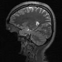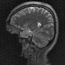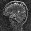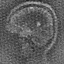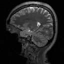Moreover, we prove that only $\mathcal{O}(|\log(\epsilon)|)$ layers are needed for an $\epsilon$-accurate solution to the inverse problem.

Deep learning (DL) has demonstrated unparalleled accomplishments in fields ranging from image classification and computer vision [34], voice recognition and automated diagnosis in medicine [29], to inverse problems and image reconstruction [32, 30, 25]. However, there is now overwhelming empirical evidence that current DL techniques typically lead to unstable methods, a phenomenon that seems universal and present in all of the applications listed above [43, 38, 3, 19, 46], and in most of the new artificial intelligence (AI) technologies. These instabilities are often detected by what has become commonly known in the literature as “adversarial attacks”. Moreover, the instabilities can be present even in random cases and not just worst-case scenarios [24] - see Figure 1 for an example of AI-generated hallucinations. There is a growing awareness of this problem in high-stake applications and society as a whole [19, 5, 26], and instability seems to be the Achilles’ heel of modern AI and DL – see Figure 2 (top row). For example, this is a problem in real-world clinical practice. Facebook and NYU’s 2019 FastMRI challenge reported that networks that performed well in terms of standard image quality metrics were prone to false negatives, failing to reconstruct small, but physically-relevant image abnormalities [33]. AI-generated hallucinations poses a serious danger in applications such as medical diagnosis. Subsequently, the 2020 FastMRI challenge [39] focused on pathologies, noting, “Such hallucinatory features are not acceptable and especially problematic if they mimic normal structures that are either not present or actually abnormal. Neural network models can be unstable as demonstrated via adversarial perturbation studies [3].”

Nevertheless, classical approximation theorems show that a continuous function can be approximated arbitrarily well by a neural network (NN). Thus, stable problems described by stable functions can always be solved stably with a NN. This leads to the following fundamental question:

Question:Why does DL lead to unstable methods and AI-generated hallucinations, even in scenarios where one can prove that stable and accurate neural networks exist?

U-net rec. from $y=Ax$	U-net rec. from $y=Ax+e_{1}$	U-net rec. from $y=Ax+e_{2}$	Original image $x$
(cropped)	(cropped)	(cropped)	(full size)
\begin{overpic}[width=433.62pt]{im_mod_118_test_nbr_003_clean_crop_131.png} \put(20.0,52.0){\color[rgb]{0,1,0}\definecolor[named]{pgfstrokecolor}{rgb}{0,1,0}\vector(1,-2){10.0}} \end{overpic}	\begin{overpic}[width=433.62pt]{im_mod_118_test_nbr_003_clean_noise_02_crop_131.png} \put(20.0,52.0){\color[rgb]{0,1,0}\definecolor[named]{pgfstrokecolor}{rgb}{0,1,0}\vector(1,-2){10.0}} \end{overpic}
FIRENET rec. from $y=Ax$	FIRENET rec. from $y=Ax+e_{1}$	FIRENET rec. from $y=Ax+e_{2}$	Original image $x$
(cropped)	(cropped)	(cropped)	(cropped)

Figure 1. (AI-generated hallucinations) A trained NN, based on a U-net architecture and trained on a set of ellipses images, generates a black area in a white ellipse (upper left image, shown as green arrow) when reconstructing the original image $x$ from noiseless measurements. By adding random Gaussian noise $e_{1}$ and $e_{2}$ (where $\|e_{1}\|_{l^{2}}/\|e_{2}\|_{l^{2}}\approx 2/5$) to the measurements, we see that the trained NN removes the aspiring black ellipse (row 1, columns 2-3). FIRENET on the other hand is completely stable with and without random Gaussian noise (row 2, cloumn 1-3 ). In the forth column, we show the original image $x$, with a red square indicating the cropped area. In this example $A\in\mathbb{C}^{m\times N}$ is a subsampled discrete Fourier transform with $m/N\approx 0.12$.

Foundations of AI for inverse problems

To answer the above question we initiate a program on the foundations of AI, determining the limits of what DL can achieve in inverse problems. It is crucial to realise that an existence proof of suitable NNs does not always imply that they can be constructed by a training algorithm. Furthermore, it is not difficult to compute stable NNs. For example, the zero network is stable, but not particularly useful. The big problem is to compute NNs that are both accurate and stable [14, 1]. Scientific computing itself is based on the pillars stability and accuracy. However, there is often a trade-off between the two. There may be barriers preventing the existence of accurate and stable algorithms, and sometimes accuracy must be sacrificed to secure stability.

Main results

We consider the canonical inverse problem of an underdetermined system of linear equations:

Given measurements $$y=Ax+e\in\mathbb{C}^{m} x\in\mathbb{C}^{N}$$, recover . (0.1)

Here, $A\in\mathbb{C}^{m\times N}$ represents a sampling model ($m<N$), such as a subsampled DFT in Magnetic Resonance Imaging (MRI). The problem in (0.1) forms the basis for much of inverse problems and image analysis. The possibility of $y\neq Ax$ models noise or perturbations. Our results demonstrate fundamental barriers preventing NNs (despite their existence) from being computed by algorithms. This helps shed light on the intricate question of why current algorithms in DL produce unstable networks, despite the fact that stable NNs often exist in the particular application. We show:

1. Theorems 1 and 2: There are well-conditioned problems (suitable condition numbers bounded by $1$) where, paradoxically, mappings from training data to suitable NNs exist, but no training algorithm (even randomised) can compute approximations of the NNs from the training data.

2. Theorem 2: The existence of algorithms computing NNs depends on the desired accuracy. For any $K\in\mathbb{Z}_{\geq 3}$, there are well-conditioned classes of problems where simultaneously: (i) algorithms may compute NNs to $K-1$ digits of accuracy, but not $K$, (ii) achieving $K-1$ digits of accuracy requires arbitrarily many training data, (iii) achieving $K-2$ correct digits requires only one training datum.

3. Theorems 3 and 4: Under specific conditions that are typically present in, for example, MRI, there are algorithms that compute stable NNs for the problem in (0.1). These NNs, which we call Fast Iterative REstarted NETworks (FIRENETs), converge exponentially in the number of hidden layers. Crucially, we prove that FIRENETs withstand adversarial attacks, see Figure 2 (bottom row), and they can even be used to stabilise unstable NNs, see Figure 3.

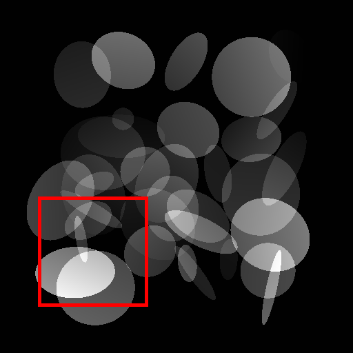
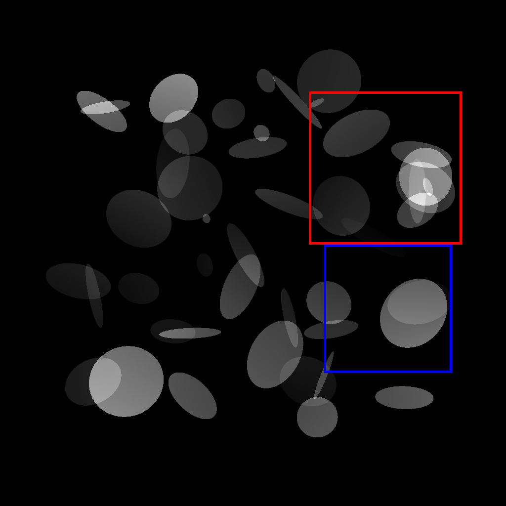
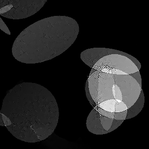
4. There is a trade-off between stability and accuracy in DL, with limits on how well a stable NN can perform in inverse problems. Figure 4 demonstrates this with a U-net trained on images consisting of ellipses and which is quite stable. However, when a detail not in the training set is added, it washes it out almost entirely. FIRENETs offer a blend of both stability and accuracy. However, they are by no means the end of the story. Tracing out the optimal stability vs. accuracy trade-off is crucial for applications and will no doubt require a myriad of different techniques to tackle different problems and stability tolerances.

$\Psi(Ax)$	$\Psi(Ax+e_{1})$	$\Psi(Ax+e_{2})$	$\Psi(Ax+e_{3})$
$\Phi(Ax)$	$\Phi(Ax+\tilde{e}_{1})$	$\Phi(Ax+\tilde{e}_{2})$	$\Phi(Ax+\tilde{e}_{3})$

Figure 2. Top row (Unstable neural network in image reconstruction): The neural network AUTOMAP (Nature (2018) [49]) represents the tip of the iceberg of DL in inverse problems. The paper promises that one can “… observe superior immunity to noise…”. Moreover, the follow-up announcement (Nature Methods “AI transforms image reconstruction,” [42]) proclaims: “A deep-learning-based approach improves speed, accuracy and robustness of biomedical image reconstruction”. However, as we see in the first row, the AUTOMAP reconstruction $\Psi(Ax+e_{j})$ from the subsampled noisy Fourier MRI data $Ax+e_{j}$, is completely unstable. Here, $A\in\mathbb{C}^{m\times N}$ is a subsampled Fourier transform, $x$ is the original image and the $e_{j}$’s are perturbations meant to simulate worst-case effect. Note that the condition number $\mathrm{cond}(AA^{*})=1$, so the instabilities are not caused by poor condition. The network weights were provided by the authors of [49] (trained on brain images from the MGH–USC HCP dataset [17]).
Bottom row (The FIRENET is stable to worst-case perturbations): Using the same method, we compute perturbations $\tilde{e}_{j}$ to simulate worst-case effect for the FIRENET $\Phi\colon\mathbb{C}^{m}\to\mathbb{C}^{N}$. As can be seen from the figure, FIRENET is stable to these worst-case perturbations. Here $x$ and $A\in\mathbb{C}^{m\times N}$ are the same image and sampling matrix as for AUTOMAP. Moreover, for each $j=1,2,3$ we have ensured that $\|\tilde{e}_{j}\|_{l^{2}}\geq\|e_{j}\|_{l^{2}}$, where the $e_{j}$’s are the perturbations for AUTOMAP (we have denoted the perturbations for FIRENET by $\tilde{e}_{j}$ to emphasise that these adversarial perturbations are sought for FIRENET and have nothing to do with the perturbations for AUTOMAP).

Fundamental barriers

We first consider basic mappings used in modern mathematics of information, inverse problems and optimisation. Given a matrix $A\in\mathbb{C}^{m\times N}$ and a vector $y\in\mathbb{C}^{m}$, we consider the following three popular minimisation problems:

$$(P_{1})\quad \operatorname{arg\!\min}_{x\in\mathbb{C}^{N}}F_{1}^{A}(x)\coloneqq\|x\|_{l^{1}_{w}},\text{ s.t. }\|Ax-y\|_{l^{2}}\!\leq\!\epsilon,$$ (0.2)

$$(P_{2})\quad \operatorname{arg\!\min}_{x\in\mathbb{C}^{N}}F_{2}^{A}(x,y,\lambda)\coloneqq\lambda\|x\|_{l^{1}_{w}}+\|Ax-y\|_{l^{2}}^{2},$$ (0.3)

$$(P_{3})\quad \operatorname{arg\!\min}_{x\in\mathbb{C}^{N}}F_{3}^{A}(x,y,\lambda)\coloneqq\lambda\|x\|_{l^{1}_{w}}+\|Ax-y\|_{l^{2}},$$ (0.4)

known respectively as quadratically constrained basis pursuit (we always assume existence of a feasible $x$ for $(P_{1})$), unconstrained LASSO and unconstrained square-root LASSO. Such sparse regularisation problems are often used as benchmarks for (0.1) and we prove impossibility results for approximations of the solution maps of $(P_{j})$. This is a striking computational barrier given that one can prove the existence of accurate neural networks (Theorem 1).

The parameters $\lambda$ and $\epsilon$ are positive rational numbers, and the weighted $l^{1}_{w}$ norm is given by $\|x\|_{l^{1}_{w}}\coloneqq\sum_{l=1}^{N}w_{l}|x_{l}|,$ where each weight $w_{j}$ is a positive rational. Throughout, we let

$$\Xi_{j}(A,y)\text{ be the set of minimisers for }(P_{j}).$$ (0.5)

Let $A\in\mathbb{C}^{m\times N}$ and let $\mathcal{S}=\{y_{k}\}_{k=1}^{R}\subset\mathbb{C}^{m}$ be a collection of samples ($R\in\mathbb{N}$). We consider the following key question:

Question: Given a collection $\Omega$ of such pairs $(A,\mathcal{S})$, does there exists a neural network approximating $\Xi_{j}$, and if so, can such an approximation be trained by an algorithm?

To make this question precise, note that $A$ and samples in $\mathcal{S}$ will typically never be exact, but can be approximated/stored to arbitrary precision. For example, this would occur if $A$ was a subsampled discrete cosine transform. Thus, we assume access to rational approximations $\{y_{k,n}\}_{k=1}^{R}$ and $A_{n}$ with

$$\|y_{k,n}-y_{k}\|_{l^{2}}\leq 2^{-n},\quad\|A_{n}-A\|\leq 2^{-n},\quad\forall n\in\mathbb{N},$$ (0.6)

where $\|\cdot\|$ refers to the usual Euclidean operator norm. The bounds $2^{-n}$ are simply for convenience and can be replaced by any other sequence converging to zero. We also assume access to rational $\left\{x_{k,n}\right\}_{k=1}^{R}$ with

$$\inf_{x^{*}\in\Xi_{j}(A_{n},y_{k,n})}\left\|x_{k,n}-x^{*}\right\|_{l^{2}}\leq 2^{-n},\quad\forall n\in\mathbb{N}.$$ (0.7)

Hence, the training set associated with $(A,\mathcal{S})\in\Omega$ for training a suitable NN must be

$$\iota_{A,\mathcal{S}}\coloneqq\left\{\left(y_{k,n},A_{n},x_{k,n}\right)\,|\,k=1,\ldots,R,\text{ and }n\in\mathbb{N}\right\}.$$ (0.8)

The class of all such admissible training data is denoted by

$$\Omega_{\mathcal{T}}\coloneqq\left\{\iota_{A,\mathcal{S}}\text{ as in \eqref{training_TT}}\,|\,(A,\mathcal{S})\in\Omega,\text{ (\ref{delt1_inf1}) and (\ref{delt1_inf2}) hold}\right\}.$$

Statements addressing the above question are summarised in the following two theorems. We use $\mathcal{N}_{m,N}$ to denote the class of NNs from $\mathbb{C}^{m}$ to $\mathbb{C}^{N}$. We use standard definitions of feedforward NNs [28], precisely given in the SI Appendix.

Theorem 1.

For any collection $\Omega$ of such $(A,\mathcal{S})$ described above, there exists a mapping

$$\mathcal{K}\colon\Omega_{\mathcal{T}}\rightarrow\mathcal{N}_{m,N},\quad\mathcal{K}(\iota_{A,\mathcal{S}})=\varphi_{A,\mathcal{S}},$$

$$\text{s.t.}\quad\varphi_{A,\mathcal{S}}(y)\in\Xi_{j}(A,y),\quad\forall y\in\mathcal{S}.$$

In words, $\mathcal{K}$ maps the training data $\Omega_{\mathcal{T}}$ to NNs that solve the optimisation problem $(P_{j})$ for each $(A,\mathcal{S})\in\Omega$.

Despite the existence of NNs guaranteed by Theorem 1, computing or training such a NN from training data is most delicate. The following is stated precisely and proven in the SI Appendix. We also include results for randomised algorithms, which are common in DL (e.g. stochastic gradient descent).

Theorem 2.

Consider the optimisation problem $(P_{j})$ for fixed parameters $\lambda\in(0,1]$ or $\epsilon\in(0,1/2]$ and $w_{l}=1$, where $N\geq 2$ and $m<N$. Let $K>2$ be a positive integer and let $L\in\mathbb{N}$. Then there exists a class $\Omega$ of elements $(A,\mathcal{S})$ as above, with the following properties. The class $\Omega$ is well-conditioned with relevant condition numbers bounded by 1 independent of all parameters. However, the following hold simultaneously (where accuracy is measured in the $l^{2}$-norm):

• ($K$ digits of accuracy impossible) There does not exist any algorithm that, given a training set $\iota_{A,\mathcal{S}}\!\in\!\Omega_{\mathcal{T}}$, produces a NN with $K$ digits of accuracy for any element of $\mathcal{S}$. Furthermore, for any $p>1/2$, no probabilistic algorithm (BSS, Turing or any model of computation) can produce a NN with $K$ digits of accuracy with probability at least $p$.

• ($K-1$ digits of accuracy possible but requires arbitrarily many training data) There does exist a deterministic Turing machine that, given a training set $\iota_{A,\mathcal{S}}\!\in\!\Omega_{\mathcal{T}}$, produces a NN accurate to $K-1$ digits over $\mathcal{S}$. However, for any probabilistic Turing machine, $M\in\mathbb{N}$ and $p\in\left[0,\frac{N-m}{N+1-m}\right)$ that produces a NN, there exists a training set $\iota_{A,\mathcal{S}}\in\Omega_{\mathcal{T}}$ such that for all $y\in\mathcal{S}$, the probability of failing to achieve $K-1$ digits or requiring more than $M$ training data is greater than $p$.

• ($K-2$ digits of accuracy possible with $L$ training data) There does exist a deterministic Turing machine that, given a training set $\iota_{A,\mathcal{S}}\in\Omega_{\mathcal{T}}$ and using only $L$ training data from each $\iota_{A,\mathcal{S}}$, produces a NN accurate to $K-2$ digits over $\mathcal{S}$.

Remark 1 (Condition).

The statement in Theorem 2 refers to standard condition numbers used in optimisation and scientific computing. For precise definitions, see the SI Appendix.

Remark 2 (Gödel, Turing, Smale and Theorem 2).

Theorem 1 and Theorem 2 demonstrate basic limitations on the existence of algorithms that can compute NNs despite their existence. This relates to Smale’s 18th problem, “What are the limits of intelligence, both artificial and human?”, from the list of mathematical problems for the 21st century [41], which echoes the famous Turing test from 1950 [45]. Smale’s discussion is motivated by the results of Gödel [22] and Turing [44] establishing impossibility results on what mathematics and digital computers can achieve [48]. Our results are actually stronger, however, than what can be obtained with Turing’s techniques. Theorem 2 holds even for any randomised Turing or Blum–Shub–Smale (BSS) machine that can solve the halting problem. It immediately opens up for a classification theory on which NNs can be computed by randomised algorithms. Theorem 3 is a first step in this direction. Below, we argue that a program on the foundations of AI, similar to Hilbert’s program on the foundations of mathematics, is needed, where impossibility results are provided in order to establish the boundaries of DL and AI.

Numerical example

To highlight the impossibility of computing NNs (Theorem 2) – despite their existence by Theorem 1 – we consider the following numerical example. Consider the problem $(P_{3})$, with $w_{l}=1$ and $\lambda=1$. Theorem 2 is stated for a specific input class $\Omega$, and in this example we consider three different such classes $\Omega_{K}$, depending on the accuracy parameter $K$. In Theorem 2, we required that $K>2$ so that $K-2>0$, but this is not necessary to show the impossibility statement (i), so we consider $K=1,3,6$. Full details of the following experiment are given in the SI Appendix.

To show that it is impossible to compute NNs which can solve $(P_{3})$ to arbitrary accuracy we consider FIRENETs $\Phi_{A_{n}}$ (the NNs in Theorem 3) and learned ISTA (LISTA) networks $\Psi_{A_{n}}$ based on the architecture choice from [11]. The networks are trained to high accuracy on training data on the form (0.8) with $R=8000$ training samples and $n$ given as in Table 1. In all cases $N=20$, $m=N-1$ and the $x_{k,n}$’s minimising $(P_{3})$ with input data $(y_{k,n},A_{n})$, are all $6$-sparse. The choice of $N$, $m$ and sparsity is to allow for fast training, other choices are certainly possible.

Table 1 shows the errors for both LISTA and FIRENETs. Both network types are given input data $(y_{n},A_{n})$, approximating the true data $(y,A)$. As is clear from the table, none of the networks are able to compute an approximation to the true minimiser in $\Xi_{3}(A,y)$ to $K$ digits accuracy. However, both networks compute an approximation with $K-1$ digits accuracy. These observations agree precisely with Theorem 2.

$\Psi_{A_{n}}$	$\Phi_{A_{n}}$	$\|A_{n}-A\|\leq 2^{-n}$ $\|y_{n}-y\|_{l^{2}}\leq 2^{-n}$	$10^{-K}$	$\Omega_{K}$
0.2999690	0.2597827	$n=10$	$10^{-1}$	$K=1$
0.3000000	0.2598050	$n=20$	$10^{-1}$	$K=1$
0.3000000	0.2598052	$n=30$	$10^{-1}$	$K=1$
0.0030000	0.0025980	$n=10$	$10^{-3}$	$K=3$
0.0030000	0.0025980	$n=20$	$10^{-3}$	$K=3$
0.0030000	0.0025980	$n=30$	$10^{-3}$	$K=3$
0.0000030	0.0000015	$n=10$	$10^{-6}$	$K=6$
0.0000030	0.0000015	$n=20$	$10^{-6}$	$K=6$
0.0000030	0.0000015	$n=30$	$10^{-6}$	$K=6$

Table 1. (Impossibility of computing approximations of the existing neural network to arbitrary accuracy). We demonstrate statement (i) from Theorem 2 on FIRENETs $\Phi_{A_{n}}$, and LISTA networks $\Psi_{A_{n}}$. The table shows the shortest $l^{2}$ distance between the output from the networks, and the true solution of the problem $(P_{3})$, with $w_{l}=1$ and $\lambda=1$, for different values of $n$ and $K$. Note that none of the networks can compute the existing correct NN (that exists by Theorem 1 and coincides with $\Xi_{3}$) to $10^{-K}$ digits accuracy, while all of them are able to compute approximations that are accurate to $10^{-K+1}$ digits (for the input class $\Omega_{K}$). This agrees exactly with Theorem 2.

The subtlety and difficulty of removing instabilities, and the need for additional assumptions

Theorem 2 shows that the problems $(P_{j})$ cannot, in general, be solved by any training algorithm. Hence any attempt at using the problems $(P_{j})$ as approximate solution maps of the general inverse problem in (0.1), without additional assumptions, is doomed to fail. This is not just the case for reconstruction using sparse regularisation, but also applies to other methods. In fact, any stable and accurate reconstruction procedure must be “kernel aware” [24], a property that most DL methods do not enforce. A reconstruction method $\Psi\colon\mathbb{C}^{m}\to\mathbb{C}^{N}$ lacks kernel awareness if it approximately recovers two vectors

$$\|\Psi(Ax)-x\|\leq\epsilon\quad\text{and}\quad\|\Psi(Ax^{\prime})-x^{\prime}\|\leq\epsilon$$ (0.9)

whose difference $\|x-x^{\prime}\|\gg 2\epsilon$ is large, but where the difference lies close to the null space of $A$ (which is non-trivial due to $m<N$) so that $\|A(x-x^{\prime})\|<\epsilon$. In particular, by applying (0.9) and the triangle inequality twice, we have that

$$\|\Psi(Ax)-\Psi(Ax^{\prime})\|\geq\|x-x^{\prime}\|-2\epsilon$$ (0.10)

implying instability, as it only requires a perturbation $e=A(x^{\prime}-x)$ of size $\|e\|<\epsilon$ for $\Psi(Ax+e)=\Psi(Ax^{\prime})$ to reconstruct the wrong image. The issue here is that if we want to accurately recover $x$ and $x^{\prime}$, i.e., we want (0.9) to hold, then we cannot simultaneously have that $x-x^{\prime}$ lies close to the kernel. Later we shall see conditions that circumvent this issue for our model class, thereby allowing us to compute stable and accurate NNs.

While training can encourage the conditions in (0.9) to hold, it is not clear how many of the defense techniques in DL, simultaneously, will protect against the condition $\|A(x-x^{\prime})\|<\epsilon$. One standard attempt to remedy instabilities is adversarial training [40]. However, while this strategy can potentially avoid (0.9), it may yield poor performance. For example, consider the following optimisation problem, which generates a reconstruction in the form of a NN given samples $\Theta=\{(y_{s},x_{s}):s=1,...,R,Ax_{s}=y_{s}\}$ and $\epsilon,\lambda>0$:

$$\min_{\phi\in\mathcal{N}_{m,N}}\!\sum_{s=1}^{R}\!\max_{\|e\|_{l^{2}}\leq\epsilon}\!\!\left\{\!\|x_{s}\!-\!\phi(y_{s})\|_{l^{2}}^{2}\!+\!\lambda\|x_{s}\!-\!\phi(y_{s}\!+\!e)\|_{l^{2}}^{2}\!\right\}\!.\!$$ (0.11)

In other words, for each training point $(y,x)\in\Theta$ we find the worst-case perturbation $e$ in the $\epsilon$-ball around $y$. This is a simplified model of what one might do using Generative Adversarial Networks (GANs) to approximate adversarial perturbations [23, 4]. For simplicity, assume that $A$ has full row rank $m$ and that we have access to exact measurements $y_{s}=Ax_{s}$. Suppose that our sample is such that $\min_{i\neq j}\|y_{i}-y_{j}\|_{l^{2}}>2\epsilon$. Any $\phi$ that minimises (0.11) must be such that $\phi(y_{s}+e)=x_{s}$ for all $e$ with $\|e\|_{l^{2}}\leq\epsilon.$ Such networks can easily be constructed using, say, ReLU activation functions. Now suppose that $x_{2}$ is altered so that $x_{1}-x_{2}$ lies in the kernel of $A$. Then for any minimiser $\phi$, we must have $\phi(y_{1}+e)=\phi(y_{2}+e)=({x_{1}+x_{2}})/{2}$ for any $e$ with $\|e\|_{l^{2}}\leq\epsilon$, and hence we can never be more than $\|x_{1}+x_{2}\|_{l^{2}}/2$ accurate over the whole test sample. Similar arguments apply to other methods aimed at improving robustness such as adding noise to training samples (known as ‘jittering’ - see Figure 4). Given such examples and Theorem 2, we arrive at the following question:

Question: Are there sufficient conditions on $A$ that imply the existence of an algorithm that can compute a neural network that is both accurate and stable for the problem in (0.1)?

Sufficient conditions for algorithms to compute stable and accurate NNs

Sparse regularisation, such as the problems $(P_{j})$, forms the core of many start-of-the-art reconstruction algorithms for inverse problems. We now demonstrate a sufficient condition (from compressed sensing) guaranteeing the existence of algorithms for stable and accurate NNs. Sparsity in levels is a standard sparsity model for natural images [2, 6] as images are sparse in levels in X-lets (wavelets, curvelets, shearlets etc.)

Definition 1 (Sparsity in levels).

Let $\text{{{M}}}=(M_{1},...,M_{r})\in{\mathbb{N}^{r}}$, $1\leq M_{1}<...<M_{r}=N$, and $\text{{{s}}}=(s_{1},...,s_{r})\in{\mathbb{N}^{r}_{0}},$ where $s_{l}\leq M_{l}-M_{l-1}$ for $l=1,...,r$ ($M_{0}=0$). $x\in\mathbb{C}^{N}$ is $(\text{{{s}}},\text{{{M}}})$-sparse in levels if $\left|\mathrm{supp}(x)\cap\{M_{l-1}+1,...,M_{l}\}\right|\leq s_{l}$ for $l=1,...,r.$ The total sparsity is $s=s_{1}+...+s_{r}$. We denote the set of $(\text{{{s}}},\text{{{M}}})$-sparse vectors by $\Sigma_{\text{{{s}}},\text{{{M}}}}$. We also define the following measure of distance of a vector $x$ to $\Sigma_{\text{{{s}}},\text{{{M}}}}$ by

$$\sigma_{\text{{{s}}},\text{{{M}}}}(x)_{l^{1}_{w}}=\inf\{\|x-z\|_{l^{1}_{w}}:z\in\Sigma_{\text{{{s}}},\text{{{M}}}}\}.$$

This model has been used to explain the effectiveness of compressed sensing [9, 16, 12] in real life applications [47, 31]. For simplicity, we assume that each $s_{l}>0$ and that $w_{i}=w_{(l)}$ if $M_{l-1}+1\leq i\leq M_{l}$ (the weights in the $l^{1}_{w}$ norm are constant in each level). For a vector $c$ which is compressible in the wavelet basis, $\sigma_{\textbf{s},\textbf{M}}(x)_{l^{1}_{w}}$ is expected to be small if $x$ is the vector of wavelet coefficients of $c$ and the levels correspond to wavelet levels [15]. In general, the weights are a prior on anticipated support of the vector [20], and we discuss some specific optimal choices in the SI Appendix.

For $\mathcal{I}\subset\{1,\ldots,N\}$, let $P_{\mathcal{I}}\in\mathbb{C}^{N\times N}$ denote the projection $(P_{\mathcal{I}}x)_{i}=x_{i}$ if $i\in\mathcal{I}$ and $(P_{\mathcal{I}}x)_{i}=0$ otherwise. The key “kernel aware” property that allows for stable and accurate recovery of $(\mathbf{s},\mathbf{M})$-spare vectors for the inverse problem (0.1), is the weighted robust null space property in levels (weighted rNSPL):

Definition 2 (weighted rNSP in levels).

Let $(\textup{{s}},\textup{{M}})$ be local sparsities and sparsity levels respectively. For weights $\{w_{i}\}_{i=1}^{N}$, $A\in\mathbb{C}^{m\times N}$ satisfies the weighted robust null space property in levels (weighted rNSPL) of order $(\textup{{s}},\textup{{M}})$ with constants $0<\rho<1$ and $\gamma>0$ if for any $(\textup{{s}},\textup{{M}})$ support set $\mathcal{I}\subset\{1,\ldots,N\}$,

$$\|P_{\mathcal{I}}x\|_{l^{2}}\leq\frac{\rho}{\sqrt{\xi}}\|P_{\mathcal{I}^{c}}x\|_{l^{1}_{w}}+\gamma\|Ax\|_{l^{2}},\quad\quad\text{for all $x\in\mathbb{C}^{N}$.}$$

We highlight that if $A$ satisfies the weighted rNSPL, then

$$\|x-x^{\prime}\|_{l^{2}}\leq C\|A(x-x^{\prime})\|_{l^{2}},\quad\forall x,x^{\prime}\in\Sigma_{\mathbf{s},\mathbf{M}},$$

where $C=C(\rho,\gamma)>0$ is a constant depending only on $\rho$ and $\gamma$ (see SI Appendix). This ensures that if $\|x-x^{\prime}\|_{\ell^{2}}\gg 2\epsilon$, then we cannot, simultaneously, have that $\|A(x-x^{\prime})\|<\epsilon$, causing the instability in (0.10). Below, we give natural examples of sampling in compressed imaging where such a property holds, for known $\rho$ and $\gamma$, with large probability. We can now state a simplified version of our result (the full version with explicit constants is given and proven in the SI Appendix):

Theorem 3.

There exists an algorithm such that for any input sparsity parameters $(\textup{{s}},\textup{{M}})$, weights $\{w_{i}\}_{i=1}^{N}$, $A\in\mathbb{C}^{m\times N}$ (with the input $A$ given by $\{A_{l}\}$) satisfying the rNSPL with constants $0<\rho<1$ and $\gamma>0$ (also input), and input parameters $n\in\mathbb{N}$ and $\{\delta,b_{1},b_{2}\}\subset\mathbb{Q}_{>0}$, the algorithm outputs a neural network $\phi_{n}$ with $\mathcal{O}(n)$ hidden layers and $\mathcal{O}(N)$ width with following property. For any $x\in\mathbb{C}^{N}$, $y\in\mathbb{C}^{m}$ with

$$\sigma_{\textup{{s}},\textup{{M}}}(x)_{l^{1}_{w}}+\|Ax-y\|_{l^{2}}\lesssim\delta,\quad\|x\|_{l^{2}}\lesssim b_{1},\quad\|y\|_{l^{2}}\lesssim b_{2},$$

we have $\|\phi_{n}(y)-x\|_{l^{2}}\lesssim{\delta}+e^{-n}.$

Hence, up to the small error term $\sigma_{\text{{{s}}},\text{{{M}}}}(x)_{l^{1}_{w}}$, as $n\rightarrow\infty$ (with exponential convergence), we recover $x$ stably with an error proportional to the measurement error $\|Ax-y\|_{l^{2}}$. The explicit constant in front of the $\|Ax-y\|_{l^{2}}$ term can be thought of as an asymptotic local Lipschitz constant for the NNs as $n\rightarrow\infty$, and thus measures stability of inexact input $y$. The error of order $\sigma_{\textup{{s}},\textup{{M}}}(x)_{l^{1}_{w}}$ measures how close the vector $x$ is from the model class of sparse in levels vectors. In the full version of Theorem 3, we also bound the error when we only approximately apply the nonlinear maps of the NNs, and show that these errors can only accumulate slowly as $n$ increases. In other words, we also gain a form of numerical stability of the forward pass of the NN. The architectures of the NNs in Theorem 3 are based on the optimisation problem $(P_{3})$ and unrolled primal-dual iterations. In addition to providing stability, the rNSPL allows us to prove exponential convergence through a careful restarting and reweighting scheme. We call our NNs Fast Iterative REstarted NETworks (FIRENETs).

Remark 3 (Unrolling does not in general yield an algorithm producing an accurate network).

Unrolling iterative methods has a rich history in DL [36, 37]. Note, however, that Theorem 2 demonstrates that despite the existence of an accurate neural network, there are scenarios where no algorithm exists that can compute it. Thus, unrolling optimisation methods can only work under certain assumptions. Our results are related to [8], which shows how key assumptions such as the robust nullspace property help bound the error of the approximation to a minimiser in terms of error bounds on the approximation to the objective function.

In the case that we do not know $\rho$ or $\gamma$ (the constants in the definition of rNSPL), we can perform a log-scale grid search for suitable parameters. By increasing the width of the NNs to $\mathcal{O}(N\log(n))$, we can still gain exponential convergence in $n$ by choosing the parameters in the grid search that lead to the vector with minimal $F_{3}^{A}$ (the objective function of $(P_{3})$). In other cases, such as Theorem 4 below, it is possible to prove probabilistic results where $\rho$ and $\gamma$ are known.

Examples in image recovery

As an application, we consider Fourier and Walsh sampling, using Haar wavelets as a sparsifying transform. Our results can also be generalised to infinite-dimensional settings via higher-order Daubechies wavelets.

Let $K=2^{r}$ for $r\in\mathbb{N}$, and set $N=K^{d}$ so that the objective is to recover a vectorised $d$-dimensional tensor $c\in\mathbb{C}^{N}$. Let $V\in\mathbb{C}^{N\times N}$ correspond to the $d-$dimensional discrete Fourier or Walsh transform (see SI Appendix). Let $\mathcal{I}\subset\{1,\ldots,N\}$ be a sampling pattern with cardinality $m=|\mathcal{I}|$ and let $D=\mathrm{diag}(d_{1},\ldots,d_{m})\in\mathbb{C}^{m\times m}$ be a suitable diagonal scaling matrix, whose entries along the diagonal depends only on $\mathcal{I}$. We assume we can observe the subsampled, scaled and noisy measurements $y=DP_{\mathcal{I}}Vc+e\in\mathbb{C}^{m}$, where projection $P_{\mathcal{I}}$ is treated as a $m\times N$ matrix by ignoring the zero entries.

To recover a sparse representation of $c$, we consider Haar wavelet coefficients. Denote the discrete $d$-dimensional Haar Wavelet transform by $\Psi\in\mathbb{C}^{N\times N}$, and note that $\Psi^{*}=\Psi^{-1}$ since $\Psi$ is unitary. To recover the wavelet coefficients $x=\Psi c$ of $c$, we consider the matrix $A=DP_{\mathcal{I}}V\Psi^{*}$, and observe that $y=Ax+e=DP_{\mathcal{I}}Vc+e$. A key result in this work is that we can design a probabilistic sampling strategy (see SI Appendix), for both Fourier and Walsh sampling in $d$-dimensions, requiring no more than $m\gtrsim(s_{1}+\ldots+s_{r})\cdot\mathcal{L}$ samples, which can ensure with high probability that $A$ satisfies the weighted rNSPL with certain constants. The sparsity in levels structure (Definition 1) is chosen to correspond to the $r$ wavelet levels. Here $\mathcal{L}$ is a logarithmic term in $N,m,s$ and $\epsilon_{\mathbb{P}}^{-1}$ (where $\epsilon_{\mathbb{P}}\in(0,1)$ is a probability). This result is crucial, as it makes $A$ kernel aware for vectors that are approximately $(\mathbf{s},\mathbf{M})$-sparse, and allows us (using Theorem 3) to design NNs which can stably and accurately recover approximately $(\mathbf{s},\mathbf{M})$-sparse vectors. Moreover, due to the exponential convergence in Theorem 3, the depth of these NNs depends only logarithmically on the error $\delta$. Below follows a simplified version of our result (the full precise version is given and proven in the SI Appendix).

Theorem 4.

Consider the above setup of recovering wavelet coefficients $x=\Psi c$ of a tensor $c\in\mathbb{C}^{K^{d}}$ from subsampled, scaled and noisy Fourier or Walsh measurements $y=DP_{\mathcal{I}}Vc+e$. Let $A=DP_{\mathcal{I}}V\Psi^{*}$, $m=|\mathcal{I}|$ and $\epsilon_{\mathbb{P}}\in(0,1)$. We then have

1. If $\mathcal{I}\subset\{1,\ldots,N\}$ is a random sampling pattern drawn according to the strategy specified in SI Appendix, and

   $$m\gtrsim(s_{1}+\cdots+s_{r})\cdot\mathcal{L}.$$

   Then with probability $1-\epsilon_{\mathbb{P}}$, $A$ satisfies the weighted rNSPL of order $(\mathbf{s},\mathbf{M})$ with constants $(\rho,\gamma)=(1/2,\sqrt{2})$. Here $\mathcal{L}$ denotes a term logarithmic in $\epsilon_{\mathbb{P}}^{-1},N,m$ and $s=\sum_{l=1}^{r}s_{l}$.

2. Suppose $\mathcal{I}$ is chosen as above. For any $\delta\in(0,1)$, let $\mathcal{J}({\delta,\mathbf{s},\mathbf{M},w})$ be the set of all $y\!=\!Ax\!+\!e\!\in\mathbb{C}^{m}$ where

   $$\|x\|_{l^{2}}\leq 1,\quad\max\left\{{\sigma_{\text{{{s}}},\text{{{M}}}}(x)_{l^{1}_{w}}},\|e\|_{l^{2}}\right\}\leq\delta.$$ (0.12)

   We provide an algorithm that constructs a neural network $\phi$ with $\mathcal{O}(\log(\delta^{-1}))$ hidden layers (and width bounded by $2(N+m)$) such that with probability at least $1-\epsilon_{\mathbb{P}}$,

   $$\left\|\phi(y)-c\right\|_{l^{2}}\lesssim\delta,\quad\forall y=Ax+e\in\mathcal{J}({\delta,\mathbf{s},\mathbf{M},w}).$$

Balancing the stability and accuracy trade-off

Current DL methods for image reconstruction can be unstable in the sense that (1) a tiny perturbation, in either the image or sampling domain, can cause severe artefacts in the reconstructed image (see Figure 2, top row), and/or (2) a tiny detail in the image domain might be washed out in the reconstructed image (lack of accuracy), resulting in potential false negatives. Inevitably, there is a stability-accuracy trade-off, for this type of linear inverse problem, making it impossible for any reconstruction method to become arbitrarily stable without sacrificing accuracy or visa versa. Here, we show that the NNs computed by our algorithm (FIRENETs) are stable with respect to adversarial perturbations and accurate for images which are sparse in wavelets. As most images are sparse in wavelets, these networks also show great generalisation properties to unseen images.

$\Psi(\tilde{y}),~{}\tilde{y}=Ax+e_{3}$	$\Phi\left(\tilde{y},\Psi(\tilde{y})\right)$	FIRENET rec. from $y=Ax+\tilde{e}_{3}$	AUTOMAP$+$FIRENET rec. from $y=Ax+\hat{e}_{3}$

Figure 3. (Adding a few FIRENET layers at the end of AUTOMAP makes it stable). The FIRENET $\Phi\colon\mathbb{C}^{m}\times\mathbb{C}^{N}\to\mathbb{C}^{N}$ takes as input measurements $y\in\mathbb{C}^{m}$ and an initial guess for $x$, which we call $x_{0}\in\mathbb{C}^{N}$. We now concatenate a 25-layer ($p=5$, $n=5$) FIRENET $\Phi$ and the AUTOMAP network $\Psi\colon\mathbb{C}^{m}\to\mathbb{C}^{N}$, by using the output from AUTOMAP as initial guess $x_{0}$, i.e., we consider the neural network mapping $y\mapsto\Phi(y,\Psi(y))$. In this experiment we consider the image $x$ from Figure 2 and the perturbed measurements $\tilde{y}=Ax+e_{3}$ (here $A$ is as in Figure 2). The first column of the figure shows the reconstruction of AUTOMAP from Figure 2. The second column shows the reconstruction of FIRENET with $x_{0}=\Psi(\tilde{y})$. The third column shows the reconstruction of FIRENET from Figure 2. The fourth column shows the reconstruction of the concatenated network with a worst case perturbation $\hat{e}_{3}$ such that $\|\hat{e}_{3}\|_{l^{2}}\geq\|e_{3}\|_{l^{2}}$. In all other experiments we set $x_{0}=0$, and consider $\Phi$ as a mapping $\Phi\colon\mathbb{C}^{m}\to\mathbb{C}^{N}$.

Adversarial perturbations for AUTOMAP and FIRENETs

Figure 2 (top row) shows the stability test of [3] applied to the AUTOMAP [49] network used for MRI reconstruction with 60% subsampling. The image $x$ seen in Figure 2 is taken from the mentioned dataset, the stability test is run on the AUTOMAP network to find a sequence of perturbations $\left|e_{1}\right|<\left|e_{2}\right|<\left|e_{3}\right|$. As can be seen from the first row in the figure, the network reconstruction completely deforms the image and the reconstruction is severely unstable (similar results for other networks are demonstrated in [3]).

In contrast, we have applied the stability test, but now for the new NNs (FIRENETs) reported in this paper. Figure 2 (bottom row) shows the results for the constructed FIRENETs, where we rename the perturbations $\tilde{e}_{j}$ to emphasise the fact that these perturbations are sought for the new NNs and have nothing to do with the adversarial perturbations for AUTOMAP. We now see that despite the search for adversarial perturbations, the reconstruction remains stable. The error in the reconstruction was also found to be at most of the same order of the perturbation (as expected from the stability in Theorem 3). In applying the test to FIRENETs, we tested/tuned the parameters in the gradient ascent algorithm considerably (much more so than was needed for applying the test to AUTOMAP, where finding instabilities was straightforward) in order to find the worst reconstruction results, yet the reconstruction remained stable. Note also that this is just one form of stability test and it is likely that there are many other tests for creating instabilities for NNs for inverse problems. This highlights the importance of results such as Theorem 3, which guarantees stability regardless of the perturbation.

To demonstrate the generalisation properties of our NNs, we show the stability test applied to FIRENETs for a range of images in the SI Appendix. This shows stability across different types of images and highlights that conditions such as Definition 2 allow great generalisation properties.

Stabilising unstable NNs with FIRENETs

Our NNs also act as a stabiliser. For example, Figure 3 shows the adversarial example for AUTOMAP (taken from Figure 2), but now shows what happens when we take the reconstruction from AUTOMAP as an input to our FIRENETs. Here we use the fact that we can view our networks as approximations of unrolled and restarted iterative methods, allowing us to use the output of AUTOMAP as an additional input for the reconstruction. We see that FIRENETs fix the output of AUTOMAP and stabilise the reconstruction. Moreover, the concatenation itself of the networks remains stable to adversarial attacks.

	Original $x$	Original	Original + detail ($x+h_{1}$)
	(full size)	(cropped, red frame)	(cropped, blue frame)
	Orig. + worst-case noise	Rec. from worst-case noise	Rec. of detail
FIRENET ($\Phi_{1}$) $(n=5,p=5)$
	Orig. + worst-case noise	Rec. from worst-case noise	Rec. of detail
Network $\Phi_{2}$ trained without noise
Network $\Phi_{3}$ trained with measurements contaminated with random noise.

Figure 4. (Trained neural networks with limited performance can be stable). We examine the accuracy/stability trade-off for linear inverse problems by considering three reconstruction networks $\Phi_{j}\colon\mathbb{C}^{m}\to\mathbb{C}^{N}$, $j=1,2,3$. Here $\Phi_{1}$ is a FIRENET, whereas $\Phi_{2}$ and $\Phi_{3}$ are the U-nets mentioned in the main text, trained without and with noisy measurements, respectively. For each network, we compute a perturbation $w_{j}\in\mathbb{C}^{N}$ meant to simulate the worst-case effect, and we show a cropped version of the perturbed images $x+w_{j}$ in the first column (row 2-4). In the middle column (row 2-4), we show the reconstructed images $\Phi_{j}(A(x+w_{j}))$ from each of the networks. In the last column (row 2-4) we test the networks’ ability to reconstruct a tiny detail $h_{1}$, in the form of the text “can u see it?”. As we see from the figure, the network trained on noisy measurements is stable to worst-case perturbations, but it is not accurate. Conversely, the network trained without noise is accurate but not stable. The FIRENET is balancing this trade-off and is accurate for images which are sparse in wavelets, and stable to worst-case perturbations.

The stability vs. accuracy trade-off and false negatives

It is easy to produce a perfectly stable network: the zero network is the obvious candidate! However, this network would obviously have poor performance and produce many false negatives. The challenge is to simultaneously ensure performance and stability. Figure 4 highlights this issue. Here we have trained two NNs to recover a set of ellipses images from noise-free and noisy Fourier measurements. The noise-free measurements are generated as $y=Ax$, where $A\in\mathbb{C}^{m\times N}$ is a subsampled discrete Fourier transform, with $m/N=0.15$ and $N=1024^{2}$. The noisy measurements are generated as $y=Ax+ce$, where $A$ is as before, and the real and imaginary components of $e\in\mathbb{C}^{m}$ are drawn from a zero mean and unit variance normal distribution $\mathcal{N}(0,1)$, and $c\in\mathbb{R}$ is drawn from the uniform distribution $\mathrm{Unif([0,100])}$. The noise $ce\in\mathbb{C}^{m}$, is generated on the fly during the training process.

The trained networks use a standard benchmarking architecture for image reconstruction, and maps $y\mapsto\phi(A^{*}y)$, where $\phi\colon\mathbb{C}^{N}\to\mathbb{R}^{N}$ is a trainable U-net NN [35, 30]. Training networks with noisy measurements, using for example this architecture, have previously been used as an example of how to create NNs which are robust towards adversarial attacks [21]. As we can see from Figure 4 (bottom row) this is the case, as it does indeed create a NN which is stable with respect to worst-case perturbations. However, a key issue is that it is also producing false negatives due to its inability to reconstruct details. Similarly, as reported in the 2019 FastMRI challenge, trained NNs that performed well in terms of standard image quality metrics were prone to false negatives: they failed to reconstruct small, but physically-relevant image abnormalities [33]. Pathologies, generalisation and AI-generated hallucinations were subsequently a focus of the 2020 challenge [39]. FIRENET, on the other hand, has a guaranteed performance (on images being sparse in wavelet bases) and stability, given specific conditions on the sampling procedure. The challenge is to determine the optimal balance between accuracy/stability, a problem that is well known in numerical analysis.

Concluding remarks

• (Algorithms may not exist – Smale’s 18th problem). There are well-conditioned problems where accurate NNs exist, but no algorithm can compute them. Understanding this phenomenon is essential in order to address Smale’s 18th problem on the limits of AI. Moreover, the limitations established in this paper suggest a classification theory describing the conditions needed for the existence of algorithms that can compute stable and accurate NNs.

• (Classifications and Hilbert’s program) The strong optimism regarding the abilities of AI is comparable to the optimism surrounding mathematics in the early 20th century, led by D. Hilbert. Hilbert believed that mathematics could prove or disprove any statement and, moreover, that there were no restrictions on which problems could be solved by algorithms. Gödel [22] and Turing [44] turned Hilbert’s optimism upside down by their foundational contributions establishing impossibility results on what mathematics and digital computers can achieve.

  Hilbert’s program on the foundations of mathematics led to a rich mathematical theory and modern logic and computer science, where substantial efforts were made to classify which problems can be computed. We have sketched a similar program for modern AI, where we provide certain sufficient conditions for the existence of algorithms to produce stable and accurate NNs. We believe that such a program on the foundations of AI is necessary and will act as an invaluable catalyst for the advancement of AI.

• (Trade-off between stability and accuracy) For ML in inverse problems there is an intrinsic trade-off between stability and accuracy. We demonstrated NNs that offer a blend of both stability and accuracy. Balancing these two interests is crucial for applications and will no doubt require a myriad of future techniques to be developed. Tracing out the optimal stability vs. accuracy trade-off remains largely an open problem, one that we expect to be of particular relevance in the increasing number of real-world implementations of ML in inverse problems.

• (Future work) Our results are just the beginning of a potential vast mathematical theory on which NNs can be computed by algorithms. Note that our sufficient conditions are just for a specific class of images. Thus, even for inverse problems, this opens up for a substantial theory covering other sufficient (and potentially necessary) conditions guaranteeing stability and accuracy, and extensions to other inverse problems such as phase retrieval [10, 18].

Methods and Data Availability

Full theoretical derivations are given in the SI Appendix. Our proof techniques for fundamental barriers in Theorem 2 stem from the SCI hierarchy that has recently been used to settle longstanding questions in scientific computing [27, 13, 7]. We introduce the concept of Sequential General Algorithms which also captures the notion of adaptive and/or probabilistic choice of training data (thus strengthening the proven lower bounds). All the code and data used to produce the figures in this manuscript are available from www.github.com/Comp-Foundations-and-Barriers-of-AI/firenet.

See pages - of SI_appendix_ARXIV.pdf

References

- [1] B. Adcock and N. Dexter. The gap between theory and practice in function approximation with deep neural networks. SIAM Journal on Mathematics of Data Science, to appear.
- [2] B. Adcock, A. C. Hansen, C. Poon, and B. Roman. Breaking the coherence barrier: A new theory for compressed sensing. In Forum of Mathematics, Sigma, volume 5. CUP, 2017.
- [3] V. Antun, F. Renna, C. Poon, B. Adcock, and A. C. Hansen. On instabilities of deep learning in image reconstruction and the potential costs of AI. PNAS, 2020.
- [4] M. Arjovsky, S. Chintala, and L. Bottou. Wasserstein generative adversarial networks. In International Conference on Machine Learning-Volume 70, pages 214–223, 2017.
- [5] N. Baker and et al. Workshop report on basic research needs for scientific machine learning: Core technologies for artificial intelligence. Technical report, USDOE Office of Science, 2019.
- [6] A. Bastounis and A. C. Hansen. On the absence of uniform recovery in many real-world applications of compressed sensing and the restricted isometry property and nullspace property in levels. SIAM J. Imaging Sci., 10(1):335–371, 2017.
- [7] A. Bastounis, A. C. Hansen, and V. Vlačić. The extended Smale’s 9th problem. Preprint, 2021.
- [8] A. Ben-Tal and A. Nemirovski. Lectures on modern convex optimization. 2020/2021.
- [9] E. J. Candes, J. K. Romberg, and T. Tao. Stable signal recovery from incomplete and inaccurate measurements. Commun. Pure Appl. Math., 59(8):1207–1223, 2006.
- [10] E. J. Candes, T. Strohmer, and V. Voroninski. Phaselift: Exact and stable signal recovery from magnitude measurements via convex programming. Communications on Pure and Applied Mathematics, 66(8):1241–1274, 2013.
- [11] X. Chen, J. Liu, Z. Wang, and W. Yin. Theoretical linear convergence of unfolded ISTA and its practical weights and thresholds. In Advances in Neural Information Processing Systems, pages 9061–9071, 2018.
- [12] A. Cohen, W. Dahmen, and R. DeVore. Compressed sensing and best -term approximation. Journal of the American mathematical society, 22(1):211–231, 2009.
- [13] M. J. Colbrook. Computing spectral measures and spectral types. Communications in Mathematical Physics, 2021.
- [14] R. DeVore, B. Hanin, and G. Petrova. Neural network approximation. arXiv preprint arXiv:2012.14501, 2020.
- [15] R. A. DeVore. Nonlinear approximation. Acta Numer., 7:51–150, 1998.
- [16] D. L. Donoho. Compressed sensing. IEEE Trans. Inf. Theory, 52(4):1289–1306, 2006.
- [17] Q. Fan et al. MGH–USC human connectome project datasets with ultra-high b-value diffusion MRI. Neuroimage, 124:1108–1114, 2016.
- [18] A. Fannjiang and T. Strohmer. The numerics of phase retrieval. Acta Numerica, pages 125–228, 2020.
- [19] S. G. Finlayson, J. D. Bowers, J. Ito, J. L. Zittrain, A. L. Beam, and I. S. Kohane. Adversarial attacks on medical machine learning. Science, 363(6433):1287–1289, 2019.
- [20] M. P. Friedlander, H. Mansour, R. Saab, and Ö. Yilmaz. Recovering compressively sampled signals using partial support information. IEEE Trans. Inf. Theory, 58(2):1122–1134, 2012.
- [21] M. Genzel, J. Macdonald, and M. März. Solving inverse problems with deep neural networks–robustness included? arXiv preprint arXiv:2011.04268, 2020.
- [22] K. Gödel. Über formal unentscheidbare Sätze der Principia Mathematica und verwandter Systeme I. Monatshefte für mathematik und physik, 38(1):173–198, 1931.
- [23] I. Goodfellow, J. Pouget-Abadie, M. Mirza, B. Xu, D. Warde-Farley, S. Ozair, A. Courville, and Y. Bengio. Generative adversarial nets. In Advances in neural information processing systems, pages 2672–2680, 2014.
- [24] N. M. Gottschling, V. Antun, B. Adcock, and A. C. Hansen. The troublesome kernel: why deep learning for inverse problems is typically unstable. arXiv preprint arXiv:2001.01258, 2020.
- [25] K. Hammernik, T. Klatzer, E. Kobler, M. P. Recht, D. K. Sodickson, T. Pock, and F. Knoll. Learning a variational network for reconstruction of accelerated MRI data. Magn. Reson. Med., 79(6):3055–3071, 2018.
- [26] R. Hamon, H. Junklewitz, and I. Sanchez. Robustness and explainability of artificial intelligence. JRC Technical Report, 2020.
- [27] A. C. Hansen. On the solvability complexity index, the -pseudospectrum and approximations of spectra of operators. J. Amer. Math. Soc., 24(1):81–124, 2011.
- [28] C. F. Higham and D. J. Higham. Deep learning: An introduction for applied mathematicians. SIAM Rev., 61(4):860–891, 2019.
- [29] G. Hinton and et al. Deep neural networks for acoustic modeling in speech recognition: The shared views of four research groups. IEEE Signal Process Mag., 29(6):82–97, 2012.
- [30] K. H. Jin, M. T. McCann, E. Froustey, and M. Unser. Deep convolutional neural network for inverse problems in imaging. IEEE Trans. Image Process., 26(9):4509–4522, 2017.
- [31] A. Jones, A. Tamtögl, I. Calvo-Almazán, and A. Hansen. Continuous compressed sensing for surface dynamical processes with helium atom scattering. Sci. Rep., 6:27776, 2016.
- [32] U. S. Kamilov, I. N. Papadopoulos, M. H. Shoreh, A. Goy, C. Vonesch, M. Unser, and D. Psaltis. Learning approach to optical tomography. Optica, 2(6):517–522, 2015.
- [33] F. Knoll et al. Advancing machine learning for MR image reconstruction with an open competition: Overview of the 2019 fastMRI challenge. Magn. Reson. Med., 2020.
- [34] A. Krizhevsky, I. Sutskever, and G. E. Hinton. Imagenet classification with deep convolutional neural networks. In Advances in neural information processing systems, pages 1097–1105, 2012.
- [35] J. Long, E. Shelhamer, and T. Darrell. Fully convolutional networks for semantic segmentation. In Proc. IEEE Comput. Soc. Conf. Comput. Vis. Pattern Recognit., pages 3431–3440, 2015.
- [36] M. T. McCann, K. H. Jin, and M. Unser. Convolutional neural networks for inverse problems in imaging: A review. IEEE Signal Process Mag., 34(6):85–95, 2017.
- [37] V. Monga, Y. Li, and Y. C. Eldar. Algorithm unrolling: Interpretable, efficient deep learning for signal and image processing. IEEE Signal Processing Magazine, 38(2):18–44, 2021.
- [38] S.-M. Moosavi-Dezfooli, A. Fawzi, and P. Frossard. Deepfool: a simple and accurate method to fool deep neural networks. In Proceedings of the IEEE Conference on Computer Vision and Pattern Recognition, pages 2574–2582, 2016.
- [39] M. J. Muckley et al. State-of-the-art Machine Learning MRI Reconstruction in 2020: Results of the Second fastMRI Challenge. arXiv preprint arXiv:2012.06318, 2020.
- [40] A. Raj, Y. Bresler, and B. Li. Improving robustness of deep-learning-based image reconstruction. In International Conference on Machine Learning, pages 7932–7942. PMLR, 2020.
- [41] S. Smale. Mathematical problems for the next century. Math. Intelligencer, 20:7–15, 1998.
- [42] R. Strack. Imaging: AI transforms image reconstruction. Nat. Methods, 15(5):309, 2018.
- [43] C. Szegedy, W. Zaremba, I. Sutskever, J. Bruna, D. Erhan, I. J. Goodfellow, and R. Fergus. Intriguing properties of neural networks. In Int. Conf. on Learning Representations, 2014.
- [44] A. Turing. On Computable Numbers, with an Application to the Entscheidungsproblem. Proc. London Math. Soc. (2), 42(3):230–265, 1936.
- [45] A. Turing. I.-Computing machinery and intelligence. Mind, LIX(236):433–460, 1950.
- [46] I. Y. Tyukin, D. J. Higham, and A. N. Gorban. On adversarial examples and stealth attacks in artificial intelligence systems. In 2020 International Joint Conference on Neural Networks (IJCNN), pages 1–6. IEEE, 2020.
- [47] Q. Wang, M. Zenge, H. E. Cetingul, E. Mueller, and M. S. Nadar. Novel sampling strategies for sparse MR image reconstruction. Proc. Int. Soc. Mag. Res. in Med., 2014.
- [48] S. Weinberger. Computers, Rigidity, and Moduli: The Large-Scale Fractal Geometry of Riemannian Moduli Space. Princeton University Press, USA, 2004.
- [49] B. Zhu, J. Z. Liu, S. F. Cauley, B. R. Rosen, and M. S. Rosen. Image reconstruction by domain-transform manifold learning. Nature, 555(7697):487, 03 2018.